STAT564/STAT476: Multivariate Analysisjames/w3-STAT576.pdf · On the previous slide, I computed the covariance directly in R using the cov function applied to the matrix Y. This matrix

3d scatterplots

You can also make 3d scatterplots, although these are less common thanscatterplot matrices.

> library(scatterplot3d)

> y <- x[,1:3]

> par(mfrow=c(2,2))

> scatterplot3d(y,highlight.3d=T,angle=20)




SAS Programming January 30, 2015 1 / 59

3d scatterplots


3d scatterplots

If you want to be really fancy you could use color to encode a fourthvariable. This would work better if the fourth dimension has a smallnumber of values (e.g., keeping track of different populations, so thatcolor could represent say, country where the individual is from).

A fifth variable could encoded by shape....but putting too muchinformation in one plot is often hard to read.


4d

Here’s an exmaple that used color to encode a fourth dimension. Theexample actually has 4 continuous dimensions.


More creative ways of displaying multiple dimensions


Correlation and Covariance

Graphs are useful for showing how variables tend to be related. Correlationquantifies the strength of the linear relationship between two variables andputs it on a scale of -1 to 1 with -1 being a perfect linear negativerelationship, +1 being a perfect linear positive relationship, and 0 being nolinear relationship.

Note that nonlinear relationships can have a correlation of 0. For example,if x = −2,−1, 0, 1, 2, and y = x2, then x and y are related by a parabola,but have a correlation of 0.


Expectation, Correlation, and Covariance

We also want to be express correlations and covariances in terms of vectorand matrix notation. We’ll start with expectation.If you have a vector of random variables

y =

y1y2. . .yp

then

E (y) =

E (y1)E (y2). . .

E (yp)

An important property of expectations for a, b, c constant and x , yrandom:

E (ax + by + c) = aE (x) + bE (y) + c

or more generally

E

(n∑

i=1

yi

)=

n∑i=1

E (yi )

Importantly, these results hold whether or not the random variablesare independent.


Expectation

We use p (rather than n) as the dimension in the previous examplebecause we are interested in p variables that are being measured. Thus thepopulation mean vector is

µ = E (y) =

y1. . .yp


Covariance

For two random varianbles, x and y , their covariance is

E [(x − E (x))(y − E (y))]

The sample covariance is

1

n − 1

n∑i=1

(xi − x)(yi − y)


Properties of the variance and covariance

For a, b, c constants and x , y random,

Var(ax + by + c) = a2Var(x) + b2Var(y) + 2abCov(x , y)

If x and y are independent, then their covariance is 0. However, if thecovariance is 0, it doesn’t follow that x and y are independent.


Correlation

The theoretical correlation between two random variables x and y is

cov(x , y)

σxσy

where σx is the standard deviation of x , equal to√

E [(x − E (x))2], andσy is the standard deviation of y .The correlation is estimated by

1n−1

∑ni=1(xi − x)(yi − y)

sxsy

where s =√

1n−1

∑ni=1(xi − x)2 is the sample standard deviation. The

correlation can be interpreted as the cosine of the angle between twovectors, which gives a mathematical explanation of why it is alwaysbetween -1 and 1.


Covariance

We want to generalize the idea of the covariance to multiple (more thantwo) random variables. The idea is to create a matrix Σ for theoreticalcovariances and S for sample covariances of pairwise covariances. Thus fora vector of random variables y, the ijth entry of S is covariance betweenvariables yi and yj . thus,

sij =1

n − 1

n∑i=1

(yij − y i )(yik − yk) =1

n − 1

(n∑

i=1

yijyik − ny iy j

)The diagonal entries of S are the sample variances. Analogous statementshold for the theoretical covariance matrix Σ.

Note that if you plug in y = x for the two-variable covariance (eithertheoretical or sample-based), you end up with the variance. Thecovariance formulas generalize the variance formulas.


Covariance

The sample covariance matrix can also be expressed in terms of theobservations (rows of the data matrix) as follows:

S =1

n − 1

n∑i=1

(yi − y)(yi − y)′

=1

n − 1

(n∑

i=1

yiy′i − n yy′

)

where y consists of the p column averages of Y, so

y =1

n

n∑i=1

y′i =

y1y2. . .yp


Covariance

The notation here is kind of confusing in terms of the number ofdimensions. Here yi refers to ith observation vector, meaning the ith rowof the data matrix. This is confusing because we used ai to refer to theith column of a matrix A.

We’ll work through an example.


Covariance: example

Suppose we have data one y1 =available soil calcium, y2 =exchangeablesoil calcium, y3 =turnip green calcium.

Location y1 y2 y31 35 3.5 2.82 35 4.9 2.73 40 30.0 4.384 10 2.8 3.215 6 2.7 2.736 20 2.8 2.817 35 4.6 2.888 35 10.9 2.909 35 8.0 3.28

10 30 1.6 3.20


Covariance: example

To calculate the sample covariance matrix, we can calculate the pairwisecovariances between each of the three variables. Then si ,j = cov(yi , yj).There are only three covariances to calculate and three variances tocalculate to determine the entire matrix S.

However, let’s also try this with using vector notation. The quantities yiwill be the ith observation, so that y2 = (35, 4.9, 2.7)′. We write this withthe transpose because we think of yi as a column vector even though it isthe ith row in the data set. Consequently, yi is 3× 1 for i = 1, . . . , 10.

y is the 3× 1 vector of means of the three columns. Thusy′ = (28.1, 7.18, 3.089)′, and we also think of y′ as a column vector.


Covariance: example

To apply the formula in the first form, we have

S =1

9

353.52.8

− 28.1

7.183.089

353.52.8

− 28.1

7.183.089

′

= + · · ·+

1

9

301.63.2

− 28.1

7.183.089

301.63.2

− 28.1

7.183.089

′


Covariance: example

Using R as a calculator (which I think is a good way to see some of thedetails of the matrix calculations),

> y1 <- c(35,3.5,2.8)

> ybar <- c(28.1,7.18,3.089)

> y1 - ybar

[1] 6.900 -3.680 -0.289

> t(y1 - ybar)

[,1] [,2] [,3]

[1,] 6.9 -3.68 -0.289

> (y1-ybar) %*% t(y1 - ybar)

[,1] [,2] [,3]

[1,] 47.6100 -25.39200 -1.994100

[2,] -25.3920 13.54240 1.063520

[3,] -1.9941 1.06352 0.083521

> y10 <- c(30,1.6,3.2)

> (y10-ybar) %*% t(y10 - ybar)

[,1] [,2] [,3]

[1,] 3.6100 -10.60200 0.210900

[2,] -10.6020 31.13640 -0.619380

[3,] 0.2109 -0.61938 0.012321

>


Covariance: example

Adding up all of these components and dividing by n − 1 (in this case 9)results in the covariance matrix

> ((y1-ybar) %*% t(y1-ybar) + (y2-ybar) %*% t(y2-ybar) + (y3-ybar) %*% t(y3-ybar)+

(y4-ybar) %*% t(y4-ybar) + (y5-ybar) %*% t(y5-ybar) + (y6-ybar) %*% t(y6-ybar)+

(y7-ybar) %*% t(y7-ybar) + (y8-ybar) %*% t(y8-ybar) + (y9-ybar) %*% t(y9-ybar)+

(y10-ybar) %*% t(y10-ybar))/9

[,1] [,2] [,3]

[1,] 140.544444 49.680000 1.9412222

[2,] 49.680000 72.248444 3.6760889

[3,] 1.941222 3.676089 0.2501211

> cov(t(Y))

[,1] [,2] [,3]

[1,] 140.544444 49.680000 1.9412222

[2,] 49.680000 72.248444 3.6760889

[3,] 1.941222 3.676089 0.2501211


Covariance: example

On the previous slide, I computed the covariance directly in R using thecov function applied to the matrix Y. This matrix could be typed in directlyor can be created by “glueing” together the y vectors. Here I typed in allof the y vectors and used the column bind function cbind in R:

Y <- cbind(y1,y2,y3,y4,y5,y6,y7,y8,y9,y10)

> Y

y1 y2 y3 y4 y5 y6 y7 y8 y9 y10

[1,] 35.0 35.0 40.00 10.00 6.00 20.00 35.00 35.0 35.00 30.0

[2,] 3.5 4.9 30.00 2.80 2.70 2.80 4.60 10.9 8.00 1.6

[3,] 2.8 2.7 4.38 3.21 2.73 2.81 2.88 2.9 3.28 3.2

which looks like the transpose of the original data. Note that for a datamatrix like this cov(Y) and cov(t(Y)) result in different matricesbecause one will be 3× 3 and the other is 10× 10. One is getting thecovariance of the column vectors and the other is getting the covariance ofthe row vectors.


Covariance

A matrix formula for the covariance is

S =1

n − 1

[Y′Y − Y′

(1

nJ

)Y

]=

1

n − 1Y′(

I− 1

nJ

)Y

This expression is mathematically concise but uses a large matrix sinceI− 1

nJ is n× n, so would require a lot of memory in the computer for largedata sets. (Mathematically equivalent expressions are not necessarilycomputationally equivalent...)

A matrix expression for the theoretical covariance is

Σ = E [(y − µ)(y − µ)′] = E (yy′)− µµ′


Correlation matrices

The correlation matrix R has entries

rij =sij√sii sjj

We can take advantage of matrices to write

Ds = diag(√s11, · · · ,

√spp) = diag(s1, . . . , sp)

andR = D−1s SD−1s

since one multiplication divides the ith row by si and the other divides thejth column by sj . From this, we also obtain

S = DsRDs

Therefore you can obtain the correlation matrix from the covariancematrix and vice versa (if you know the sample variances).


Partitioned vectors and matrices

If a vector is partitioned into two sets of variables, sayy1, . . . , yp, x, . . . , xq, then we can compute expected values, covariancesand correlations using partitioned matrices. We have

E

(yx

)=

(E (y)E (x)

)

cov

(yx

)= Σ =

(Σyy Σyx

Σxy Σxx

)Here Σyy is the covariance matrix of the y variables only, Σyx has thecovariances of the y variables versus the x variables, and Σxx is thecovariance matrix of the x variables. For this matrix, Σyx = Σ′xy .


Partitioned vectors

Note that if x and y are independent, then Σxy = 0, and the covariancematrix has block diagonal structure.

This structure could arise when you have measurements on differentfamilies, where different families are assumed to be independent, butindividuals within families are not independent of one another formeasurements like height, weight, age, blood pressure, etc.

For more than two families, you’d want to partition your random variablesinto multiple sets (one for each family), and you can work with partitionedvectors and matrices that generalizes the case of two partitions.


Linear combinations of variables

Sometimes we want to work with a linear combination of variables. Forexample, in Galton’s data set, you could have each row contain a familyand the columns could be the y1 = height of the son, y2 = height of thefather, and y3 = height of the mother. Galton used the average of thefather’s height and 1.08 times the mother’s height. So Galton wasinterested in the relationship between y1 and (y2 + 1.08y3)/2.

More generally, if you have variables y1, . . . , yp, then the linear combination

z = a1y1 + · · · apyp

can be written asz = a′y



If we let the ith observation and jth variable be yij , then the ith linearcombination is

zi =

p∑j=1

ajyij = a′yi

where yi is the ith observation vector (row in the data set), but is treatedas a column vector. Since a and yi are p × 1, zi is 1× 1.



The average of the linear combinations is

z =1

n

n∑i=1

zi = a′y

Recall that y is a vector of the p column averages of the data set. Thus,we can compute the average using the zi terms or directly from theoriginal data.Similarly, the sample variance of the zi terms is

s2z =1

n − 1

n∑i=1

(zi − z)2 = a′Sa



Here, if you have a univariate random variable y , then var(ay) = a2var(y).This true for both theoretical variances and sample variances (if youmultiple all samples by a, the sample variance is multiplied by a factor a2).The matrix analogue for this is that

var(a′y) = a′var(y)a

Again, the result is a scalar (single real number), and the same ideaapplies to both the sample variance and theoretical variance, so you canreplace var(y) with either S or Σ.



Because s2z = 1n−1

∑ni=1(zi − z)2 ≥ 0, it’s also the case that a′Sa ≥ 0, and

therefore this shows that S is positive semidefinite, and positive denitenessholds (meaning the inequality is strict) with probability 1 if n − 1 > p andthe variables are continuous.

In practice, the probability 1 result won’t hold because our measurementshave finite precision, so you could get unlikely and end up with acovariance matrix that wasn’t full rank. Statements claiming thatsomething holds with probability 1 mean that there are outcomes in thesample space where the condition wouldn’t hold, but this events haveprobability 0. For example, if x and y are both standard normal, then theevent that x = 0 and y = 0 could occur based on the underlying samplespace, yet P(x = y = 0) = 0.



If w = b′y is a second linear combination, then z and w are two distinctrandom variables which might or might not be correlated. Theircovariance is

szw =

∑ni=1(zi − z)(wi − w)2

n − 1= a′Sb

and the sample correlation is

rzw =szwszsw

=a′Sb√

a′Sa√

b′Sb


Extensions to more than two variables

If you want to transform your n × p data matrix into something that is,say n × k with k < p, then you can transform your data with a matrixmultiplication. Let

zi = Ayi

Here A is k × p and yi is p× 1, so zi is k × 1. The point of doing this is toreduce the dimension of your statistical problem, or to remove collinearityin your variables that could cause problems for some statistical procedures.In some cases we also use k = p, to rotate the data in a useful way.You could also use

zi = Ayi + b

for a more general transformation.


Extensions to more than two variables.

The previous results generalize well to this type of problem with

z = Ay + b

Sz = ASA′

Theoretical covariances can replace sample covariances by substituting Σfor S:

E (Ay + b) = AE (y) + b

cov(Ay + b) = AΣA′


Measures of overall variability

To measure the overall variability in a sample, you can use thegeneralized sample variance, det(S) = |S| and the trace, tr(S).

The trace gives the sum of the individual sample variances, and thereforeignores covariances. On the other hand |S| will be 0 (or near 0) if there ismulticollinearity (or near multicollinearity) in the data. Otherwise, largevalues of either of these statistics suggest that the observations are notclose to the mean vector y. The book says that y1, . . . , yp are not close toy, but this appears to be a typo, and it should say y1, . . . , yn instead, sincethe issue is whether the observations are close to the average observation.


Distance between vectors

In univariate statistics, you might be interested in seeing whether a valueis unusual. For example, to see how unusual it is for someone to be say, 76inches tall (6 foot 4), knowing the mean value (say 70 inches) only tells usthat the person is 6 inches above average in height, but not how unusualthis is.

To measure how unusual an observation is, we get the z-score, whichstandardizes the observation:

z =x − µσ

= (x − µ)σ−1

or we estimate using

z =x − x

s= (x − x)s−1


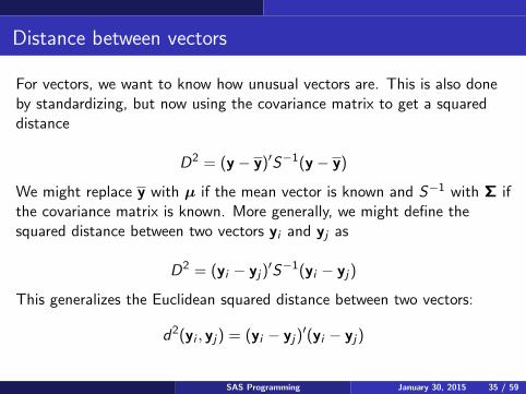
Distance between vectors

For vectors, we want to know how unusual vectors are. This is also doneby standardizing, but now using the covariance matrix to get a squareddistance

D2 = (y − y)′S−1(y − y)

We might replace y with µ if the mean vector is known and S−1 with Σ ifthe covariance matrix is known. More generally, we might define thesquared distance between two vectors yi and yj as

D2 = (yi − yj)′S−1(yi − yj)

This generalizes the Euclidean squared distance between two vectors:

d2(yi , yj) = (yi − yj)′(yi − yj)


Mahalanobis distance

The squared distances are often called (squared) Mahalanobis distances,who proposed them in 1936. The idea is that the similarity between twovectors can take into account the variability in some of the dimensions notbeing equal. For example, if I measure blood pressure on individuals, thenthe systolic blood pressure (the higher number) might be more variablethan the lower number. So, if I compare three blood pressures:

Individual systolic diastolic

1 120 802 130 753 140 854 150 90


Mahalanobis distance

In this case y = (135, 82.5)′. Individuals 1 and 2 have squared Euclideandistance from the mean of√

(120− 135)2 + (80− 82.5)2 = 15.2√(130− 135)2 + (75− 82.5)2 = 12.5

Based on their Mahalanobis distances, the two individuals are equallydistant from the mean vector y = (135, 82.5)′. The reason is that thediastolic blood pressure is more variable and being different from the meandiastolic pressure counts less than being different from the mean systolicblood pressure.


Mahalanobis distance in R

Here’s how to calculate the Mahalanobis distances in R for this example:

> x <- c(120,130,140,150,80,75,85,90)

> x <- matrix(x,ncol=2,byrow=F)

> mu <- c(mean(x[,1]),mean(x[,2]))

> sqrt(t(x[1,]-mu) %*% solve(cov(x)) %*% (x[1,]-mu))

[,1]

[1,] 1.47196


[,1]

[1,] 1.47196


[,1]

[1,] 0.4082483

> sqrt(mahalanobis(x,mu,cov(x)))

[1] 1.4719601 1.4719601 0.4082483 1.2247449


Distances between vectors

Distances are obtained by taking square roots of these squared distances.Mathematically a distance function d satisfies

d(x , y) ≥ 0 with equality if and only if x = y

d(x , y) = d(y , x) (symmetry)

d(x , y) + d(y , z) ≥ d(x , z) (triangle inequality)

Note that squared distances are not always distances because they can failto satisfy the triangle inequality. Sometimes functions that fail the triangleinequality but satisfy the other two properties are called dissimilaritymeasures and are useful in statistics also.


Example of a squared distance not being a distance

Let f (a, b) = (a− b)2, where a and b are real numbers. Then let a = 0.1,b = 0.2, c = 0.4. Then

f (a, b) + f (b, c) = 0.01 + 0.04 = 0.05, f (a, c) = 0.09 > f (a, b) + f (b, c)

Since f doesn’t satisfy the triangle inequality, it is not a distance.However, it could still be used as a measure of dissimilarity.s On the other hand,

g(a, b) = | log(a)− log(b)|

does define a metric.


Chapter 4: Multivariate Normal Distribution

Just as many statistical methods developed for a univariate responseassume normality, many multivariate methods extend the univariatenormal distribution to a multivariate normal distribution.

The simplest case is the bivariate normal distribution, in which there aretwo random variables, say y1 and y2, which are correlated. In the bivariatecase, the joint distribution of y1 and y2 has 5 parameters: µ1, µ2, σ1 (orσ21), σ2 (or σ22), plus ρ, the correlation between y1 and y2.

We’ll quickly want to generalize this to more than two random variables.Instead of a correlation, a vector of random variables y is characterized bya vector of means µ, and a covariance matrix Σ, which includes thevariances of the individual variables as well as the covariances.


The normal distribution

The univariate normal has density function

f (y) =1√

2πσ2e−(y−µ)

2/(2σ2)

It is very common to see this written as

f (y) =1√

2πσ2e−(y−µ)

2/2σ2

without the parentheses in the denominator in the exponent. It is commonto see both forms, and the textbook uses the first form. However, theorder of operations here isn’t very clear. Keep in mind that if you type

exp(-(y-mu)^2/2*sigma^2)

In R, you will get the wrong number, and

exp(-(y-mu)^2/(2*sigma^2))

will be correct.SAS Programming January 30, 2015 42 / 59

The normal distrbution

The normal distribution goes by several names: The normal, the bellcurve, the Gaussian, and it is related to the error function

erf(t) =

∫ x

0e−t

2dt

Different names are common in different disciplines; for example Gaussianis often used in engineering. I see this as being like Gandalf from the Lordof the Rings and The Hobbit. He is a central character in the stories andmany things to different people, so he gets many names: Gandalf the Grey,Gandalf the White, Mithrandir, Greybeard, Olorin, ...

The normal distribution is like the Gandalf of Statistics...


The bivariate normal distribution

The bivariate normal looks like a hill. The total variance, |Σ| afffects howpeaked or spread out the distribution is, while the correlation (orcovariance) terms affect how symmetrical the distribution is.



The bivariate normal looks like a hill. The total variance, |Σ| afffects howpeaked or spread out the distribution is, while the correlation (orcovariance) terms affect how symmetrical the distribution is.





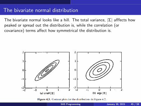
The bivariate normal density is manageable to write down without usingmatrices. For more than two variables, we’ll use matrix notation, whichcan also be used in the two variable case. For two variables, the density is

f (y1, y2) =1

2πσ1σ2√

1− ρ2exp

[z

2(1− ρ2)

]where

z =(y1 − µ1)2

σ21− 2ρ(y1 − µ1)(y2 − µ)

σ1σ2+

(y2 − µ2)2

σ22

andρ = cov(y1, y2)/(σ1σ2)



If you let yi = yi−µiσi

, then you can write the bivaraite density using

z = y12 − 2ρ y1y2 + y2

2

so

f (y1, y2) =1

2πσ1σ2√

1− ρ2exp

[y1

2 − 2ρ y1y2 + y22

2(1− ρ2)

]


The multivariate normal distribution

To express this in matrix and vector form, and to generalize to more thantwo variables, we write

f (y) =1

(√

2π)p|Σ|1/2exp

[−(y − µ)′Σ−1(y − µ)/2

]Note that

(y − µ)′Σ−1(y − µ)

is the square of the Mahalanobis distance between y and µ.


The multivariate normal and bivariate normal

We might want to check that this is equivalent to the expression we hadfor the bivariate normal with p = 2. To do this, recall that for a 2× 2matrix

A−1 =1

a11a22 − a12a21

(a22 −a12−a21 a11

)so

Σ−1 =1

σ21σ22 − σ212

(σ22 −σ12−σ12 σ21

)


The multivariate normal and bivariate normal

After multiplying, we get

(y − µ)′Σ−1(y − µ)/2

=σ22(y1 − µ1)2 − 2σ12(y1 − µ1)(y2 − µ2) + σ21(y2 − µ2)2

2(σ21σ22 − σ212)

With a little manipulation, we can show that this is equivalent to the firstversion of the bivariate density that we showed.


Properties of the multivariate normal

We can write that a vector is multivariate normal as y ∼ Np(µ,Σ).Some important properties of multivariate normal distributions include

1. Linear combinations of the variables y1, . . . , yp are also normal withNote that for some distributions, such as the Poisson, sums of independent(but not necessarily identically distributed) random variables stay withinthe same family of distributions. For other distributions, they don’t stay inthe same family (e.g., exponential random variables). However, it is notclear that sums of two correlated Poissons will still be Poisson. Also,differences between Poisson random variables are not Poisson. For thenormal, we have the nice property that even if two (or more) normalrandom variables are correlated, any linear combinations will still benormal.


Properties of multivariate normal distributions

2. If A is constant (entries are not random variables) and is q × p withrank q ≤ p, then

Ay ∼ Nq(Aµ,AΣA′)

What happens if q > p?



3. A vector y can be standardized using either

z = (T′)−1(y − µ)

where T is obtained using the Cholesky decomposition so that T′T = Σ,or

z = (Σ1/2)−1(y − µ)

This standardization is similar to the idea of z-scores; however, just takingthe usual z-scores of the individual variables in y will still leave thevariables correlated. The standardizations above result in

z ∼ Np(0, I)



4. Sums of squares of p independent standard normal random variableshave a χ2 distribution with p degrees of freedom. Therefore, ify ∼ Np(µ,Σ), then

(y − µ)′Σ−1(y − µ) = (y − µ)′(

Σ1/2Σ1/2)−1

(y − µ)

= (y − µ)′(

Σ1/2)−1 (

Σ1/2)−1

(y − µ)

=

[(Σ1/2

)−1(y − µ)

]′ (Σ1/2

)−1(y − µ)

= z′z

Here the vector z consists of i.i.d. standard normal vectors according toproperty 3, so z′z is a sum of squared i.i.d. standard normals, which isknown to have χ2 distribution. Therefore

(y − µ)′Σ−1(y − µ) ∼ χ2p



5. Normality of marginal distributions

If y has p random variables and is multivariate normal, then any subsetyi1 , . . . , yir , r < p, is also multivariate normal. We can assume that the rvariables of interested are listed first so that

y1 = (y1, . . . , yr )′, y2 = (yr+1, . . . , yp)′

Then we have

y =

(y1y2

), µ =

(µ1

µ2

), Σ =

(Σ11 Σ12

Σ21 Σ22

)and

y1 ∼ Nr (µ1,Σ11)


Marginal distributions

If you have a collection of random variables, and you ignore some of them,the distribution of the remaining is a marginal distribution. For a bivariaterandom variable y = (y1, y2)′, the distribution of y1 is a marginaldistribution of the distribution of y.In non-vector notation, the joint density for two random variables is oftenwritten

f12(y1, y2)

and the marginal distribution can be obtained by

f1(y1) =

∫ ∞−∞

f (y1, y2) dy2

The joint density for y1 is

f1(y1, . . . , yr ) =

∫ ∞−∞· · ·∫ ∞−∞

f (y1, . . . , yp) dyr+1 · · · dyp

And this is why it is called a marginal density.SAS Programming January 30, 2015 57 / 59

Plotting marginal densities in R

> install.packages("ade4")

> library(ade4)

> x <- rnorm(100)

> y <- x+ rnorm(100)

> d <- data.frame(x,y)

> s.hist(d)


Plotting marginal densities in R


Documents

STAT564/STAT476: Multivariate Analysisjames/w3-STAT576.pdf · On the previous slide, I computed the covariance directly in R using the cov function applied to the matrix Y. This matrix