Embed Size (px)
Citation preview

C.I.D.E.
CENTRO INTERDIPARTIMENTALE DI DOCUMENTAZIONE ECONOMICA
UNIVERSITÀ DEGLI STUDI DI VERONA
Manuale di Stata...ovvero una informale introduzione a Stata
con l’aggiunta di casi applicati
Author:NICOLA TOMMASI
3 febbraio 2009rev. 0.08

Info
Sito web: http://www.stata.com/Mailing list: http://www.stata.com/statalist/archive/
dott. Nicola Tommasie-mail: [email protected] - [email protected].: 045 802 80 48 (p.s. niente cellulare, non lo possiedo. La mail è lostrumento migliore e con probabilità più elevata per contattarmi).
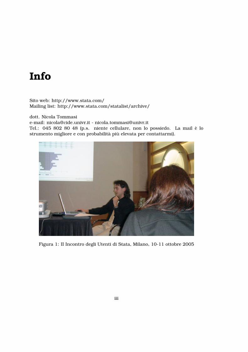
Figura 1: II Incontro degli Utenti di Stata, Milano, 10-11 ottobre 2005
iii


Indice
Info iii
Indice v
Ringraziamenti ix
Lista delle modifiche xi
Introduzione xiii
I Manuale 1
1 Descrizione di Stata 31.1 La disposizione delle finestre . . . . . . . . . . . . . . . . . . . . . . 31.2 Limiti di Stata . . . . . . . . . . . . . . . . . . . . . . . . . . . . . . 5
2 Convenzioni Tipografiche 9
3 La Filosofia del Programma 113.1 Schema di funzionamento . . . . . . . . . . . . . . . . . . . . . . . 12
4 Organizzare il Lavoro 154.1 Organizzazione per cartelle di lavoro . . . . . . . . . . . . . . . . . 154.2 Interazione diretta VS files .do . . . . . . . . . . . . . . . . . . . . . 174.3 Registrazione dell'output . . . . . . . . . . . . . . . . . . . . . . . . 184.4 Aggiornare il programma . . . . . . . . . . . . . . . . . . . . . . . . 194.5 Aggiungere comandi . . . . . . . . . . . . . . . . . . . . . . . . . . . 204.6 Fare ricerche . . . . . . . . . . . . . . . . . . . . . . . . . . . . . . . 214.7 Cura dei dati . . . . . . . . . . . . . . . . . . . . . . . . . . . . . . . 234.8 Intestazione file .do . . . . . . . . . . . . . . . . . . . . . . . . . . . 25
5 Alcuni Concetti di Base 275.1 L’input dei dati . . . . . . . . . . . . . . . . . . . . . . . . . . . . . . 27
v
INDICE INDICE
5.1.1 Caricamento dei dati in formato proprietario . . . . . . . . . 275.1.2 Caricamento dei dati in formato testo . . . . . . . . . . . . . 275.1.3 Caricamento dei dati in altri formati proprietari (StatTrans-
fer) . . . . . . . . . . . . . . . . . . . . . . . . . . . . . . . . . 285.2 Regole per denominare le variabili . . . . . . . . . . . . . . . . . . . 285.3 Il qualificatore in . . . . . . . . . . . . . . . . . . . . . . . . . . . . . 295.4 Il qualificatore if . . . . . . . . . . . . . . . . . . . . . . . . . . . . . 305.5 Operatori di relazione . . . . . . . . . . . . . . . . . . . . . . . . . . 315.6 Operatori logici . . . . . . . . . . . . . . . . . . . . . . . . . . . . . . 325.7 Caratteri jolly e sequenze . . . . . . . . . . . . . . . . . . . . . . . . 325.8 L’espressione by . . . . . . . . . . . . . . . . . . . . . . . . . . . . . 335.9 Dati missing . . . . . . . . . . . . . . . . . . . . . . . . . . . . . . . 34
6 Il Caricamento dei Dati 376.1 Dati in formato proprietario (.dta) . . . . . . . . . . . . . . . . . . . 376.2 Dati in formato testo . . . . . . . . . . . . . . . . . . . . . . . . . . 41
6.2.1 Formato testo delimitato . . . . . . . . . . . . . . . . . . . . 416.2.2 Formato testo non delimitato . . . . . . . . . . . . . . . . . . 42
6.3 Altri tipi di formati . . . . . . . . . . . . . . . . . . . . . . . . . . . . 456.4 Esportazione dei dati . . . . . . . . . . . . . . . . . . . . . . . . . . 466.5 Cambiare temporaneamente dataset . . . . . . . . . . . . . . . . . 47
7 Gestione delle Variabili 517.1 Descrizione di variabili e di valori . . . . . . . . . . . . . . . . . . . 517.2 Controllo delle variabili chiave . . . . . . . . . . . . . . . . . . . . . 617.3 Rinominare variabili . . . . . . . . . . . . . . . . . . . . . . . . . . . 627.4 Ordinare variabili . . . . . . . . . . . . . . . . . . . . . . . . . . . . 637.5 Prendere o scartare osservazioni o variabili . . . . . . . . . . . . . 647.6 Gestire il formato delle variabili . . . . . . . . . . . . . . . . . . . . 66
8 Creare Variabili 698.1 Il comando generate . . . . . . . . . . . . . . . . . . . . . . . . . . 69
8.1.1 Funzioni matematiche . . . . . . . . . . . . . . . . . . . . . . 698.1.2 Funzioni di distribuzione di probabilità e funzioni di densità 718.1.3 Funzioni di generazione di numeri random . . . . . . . . . . 738.1.4 Funzioni stringa . . . . . . . . . . . . . . . . . . . . . . . . . 738.1.5 Funzioni di programmazione . . . . . . . . . . . . . . . . . . 768.1.6 Funzioni data . . . . . . . . . . . . . . . . . . . . . . . . . . . 778.1.7 Funzioni per serie temporali . . . . . . . . . . . . . . . . . . 788.1.8 Funzioni matriciali . . . . . . . . . . . . . . . . . . . . . . . . 78
8.2 Lavorare con osservazioni indicizzate . . . . . . . . . . . . . . . . . 818.3 Estensione del comando generate . . . . . . . . . . . . . . . . . . 838.4 Sostituire valori in una variabile . . . . . . . . . . . . . . . . . . . . 868.5 Creare variabili dummy . . . . . . . . . . . . . . . . . . . . . . . . . 90
vi Nicola Tommasi
INDICE INDICE
9 Analisi Quantitativa 939.1 summarize e tabulate . . . . . . . . . . . . . . . . . . . . . . . . . 93
9.1.1 Qualcosa di più avanzato . . . . . . . . . . . . . . . . . . . . 1049.2 Analisi della correlazione . . . . . . . . . . . . . . . . . . . . . . . . 1089.3 Analisi outliers . . . . . . . . . . . . . . . . . . . . . . . . . . . . . . 109
10 Trasformare Dataset 11510.1Aggiungere osservazioni . . . . . . . . . . . . . . . . . . . . . . . . . 11510.2Aggiungere variabili . . . . . . . . . . . . . . . . . . . . . . . . . . . 11610.3Collassare un dataset . . . . . . . . . . . . . . . . . . . . . . . . . . 12310.4reshape di un dataset . . . . . . . . . . . . . . . . . . . . . . . . . 12410.5Contrarre un dataset . . . . . . . . . . . . . . . . . . . . . . . . . . 128
11 Lavorare con Date e Orari 13111.1La teoria . . . . . . . . . . . . . . . . . . . . . . . . . . . . . . . . . . 13111.2Visualizzazione delle date e delle ore . . . . . . . . . . . . . . . . . 13411.3Ricavare date da variabili stringa . . . . . . . . . . . . . . . . . . . 13611.4Visualizzazione delle ore . . . . . . . . . . . . . . . . . . . . . . . . 13711.5Operazioni con date e ore . . . . . . . . . . . . . . . . . . . . . . . . 137
12 Macros e Cicli 13912.1Macros . . . . . . . . . . . . . . . . . . . . . . . . . . . . . . . . . . . 13912.2I cicli . . . . . . . . . . . . . . . . . . . . . . . . . . . . . . . . . . . . 141
13 Catturare Informazioni dagli Output 147
14 Mappe 151
II Casi Applicati 159
15 Dataset di Grandi Dimensioni 161
16 Da Stringa a Numerica 16516.1Fondere variabili stringa con numeriche . . . . . . . . . . . . . . . 16516.2Da stringa a numerica categorica . . . . . . . . . . . . . . . . . . . 168
17 Liste di Files e Directory 169
18 Previsioni Multiple 17518.1Introduzione . . . . . . . . . . . . . . . . . . . . . . . . . . . . . . . 17518.2La stima del modello . . . . . . . . . . . . . . . . . . . . . . . . . . . 175
19 reshape su Molte Variabili 187
Nicola Tommasi vii

INDICE INDICE
III Appendici 191
A spmap: Visualization of spatial data 193A.1 Syntax . . . . . . . . . . . . . . . . . . . . . . . . . . . . . . . . . . . 193
A.1.1 basemap_options . . . . . . . . . . . . . . . . . . . . . . . . . 193A.1.2 polygon_suboptions . . . . . . . . . . . . . . . . . . . . . . . 194A.1.3 line_suboptions . . . . . . . . . . . . . . . . . . . . . . . . . . 195A.1.4 point_suboptions . . . . . . . . . . . . . . . . . . . . . . . . . 195A.1.5 diagram_suboptions . . . . . . . . . . . . . . . . . . . . . . . 196A.1.6 arrow_suboptions . . . . . . . . . . . . . . . . . . . . . . . . 197A.1.7 label_suboptions . . . . . . . . . . . . . . . . . . . . . . . . . 198A.1.8 scalebar_suboptions . . . . . . . . . . . . . . . . . . . . . . . 199A.1.9 graph_options . . . . . . . . . . . . . . . . . . . . . . . . . . 199
A.2 description . . . . . . . . . . . . . . . . . . . . . . . . . . . . . . . . 199A.3 Spatial data format . . . . . . . . . . . . . . . . . . . . . . . . . . . 200A.4 Color lists . . . . . . . . . . . . . . . . . . . . . . . . . . . . . . . . . 206A.5 Choropleth maps . . . . . . . . . . . . . . . . . . . . . . . . . . . . . 207A.6 Options for drawing the base map . . . . . . . . . . . . . . . . . . . 209A.7 Option polygon() suboptions . . . . . . . . . . . . . . . . . . . . . . 212A.8 Option line() suboptions . . . . . . . . . . . . . . . . . . . . . . . . . 213A.9 Option point() suboptions . . . . . . . . . . . . . . . . . . . . . . . . 214A.10Option diagram() suboptions . . . . . . . . . . . . . . . . . . . . . . 217A.11Option arrow() suboptions . . . . . . . . . . . . . . . . . . . . . . . 219A.12Option label() suboptions . . . . . . . . . . . . . . . . . . . . . . . . 221A.13Option scalebar() suboptions . . . . . . . . . . . . . . . . . . . . . . 223A.14Graph options . . . . . . . . . . . . . . . . . . . . . . . . . . . . . . 223A.15Acknowledgments . . . . . . . . . . . . . . . . . . . . . . . . . . . . 251
B Lista pacchetti aggiuntivi 255
To Do 273
IV Indici 275
Indice Analitico 277
Elenco delle figure 281
Elenco delle tabelle 283
viii Nicola Tommasi

Ringraziamenti
Molto del materiale utilizzato in questo documento proviene da esperienze per-sonali. Prima e poi nel corso della stesura alcune persone mi hanno aiutatoattraverso suggerimenti, insegnamenti e correzioni; altre hanno contribuito inaltre forme. Vorrei ringraziare sinceramente ciascuno di loro. Naturalmentetutti gli errori che troverete in questo libro sono miei.
Li elenco in ordine rigorosamente sparso
Fede che mi ha fatto scoprire Stata quando ancora non sapevo accendereun PCRaffa con cui gli scambi di dritte hanno contribuito ad ampliare le mieconoscenzePiera che mi dato i primissimi rudimenti
ix

Lista delle modifiche
rev. 0.01
- Prima stesura
rev. 0.02
- Aggiunti esempi di output per illustrare meglio i comandi- Aggiornamenti dei nuovi comandi installati (adoupdate)- Controllo delle variabili chiave (duplicates report)
rev. 0.03
- Aggiunti esempi di output per illustrare meglio i comandi- Conversione del testo in LATEX (così lo imparo)- Creata la sezione con i casi applicati
rev. 0.04
- Indice analitico- Mappe (comando spmap, ex tmap- Ulteriori esempi
rev. 0.06
- Correzioni varie- Date e ore- Ulteriori casi applicati
xi


Introduzione
Questo è un tentativo di produrre un manuale che integri le mie esperienzenell’uso di Stata. È un work in progress in cui di volta in volta aggiungo nuovicapitoli, integrazioni o riscrivo delle parti. In un certo senso è una collezionedelle mie esperienze di Stata, organizzate per assomigliare ad un manuale, contutti i pro e i contro di una tale genesi.Non è completo come vorrei ma il tempo è un fattore limitante. Se qualcunovuole aggiungere capitoli o pezzi non ha che da contattarmi, sicuramente tro-veremo il modo di inglobare i contributi che verranno proposti. Naturalmentesiete pregati di segnalarmi tutti gli errori che troverete (e ce ne saranno).
Questo documento non è protetto in alcun modo contro la duplicazione. La of-fro gratuitamente a chi ne ha bisogno senza restrizioni, eccetto quelle impostedalla vostra onestà. Distribuitela e duplicatela liberamente, basta che:
- il documento rimanga intatto- non lo facciate pagare
Il fatto che sia liberamente distribuibile non altera né indebolisce in alcunmodo il diritto d’autore (copyright), che rimane mio, ai sensi delle leggi vigenti.
xiii


Parte I
Manuale
1


Capitolo 1
Descrizione di Stata
Software statistico per la gestione, l’analisi e la rappresentazione grafica di dati
Piattaforme supportate
- Windows (versioni 32 e 64 bit)- Linux (versioni 32 e 64 bit)- Macintosh- Unix, AIX, Solaris Sparc
Versioni (in senso crescente di capacità e potenza)
- Small Stata- Stata/IC- Stata/SE- Stata/MC
La versione SE è adatta alla gestione di database di grandi dimensioni. La ver-sione MP è ottimizzata per sfruttare le architetture multiprocessore attraver-so l’esecuzione in parallelo dei comandi di elaborazione (parallelizzazione delcodice). Per farsi un’idea si veda l’ottimo documento reperibile qui:Stata/MP Performance Report(http://www.stata.com/statamp/report.pdf)Questa versione, magari in abbinamento con sistemi operativi a 64bit, è par-ticolarmente indicata per situazioni in cui si devono elaborare grandi quantitàdi dati (dataset di svariati GB) in tempi che non siano geologici.
1.1 La disposizione delle finestre
Stata si compone di diverse finestre che si possono spostare ed ancorare aproprio piacimento (vedi Figura 1.1). In particolare:
3

1.1. La disposizione delle finestre 1. Descrizione di Stata
1. Stata Results: finestra in cui Stata presenta l’output dei comandi impar-titi
2. Review: registra lo storico dei comandi impartiti dalla Stata Command.Cliccando con il mouse su uno di essi, questo viene rinviato alla StataCommand
3. Variables: quando un dataset è caricato qui c’è l’elenco delle variabili chelo compongono
4. Stata Command: finestra in cui si scrivono i comandi che Stata deveeseguire
A partire dalla versione 8 è possibile eseguire i comandi anche tramite la bar-ra delle funzioni dove sotto 'Data', 'Graphics' e 'Statistics' sono raggruppati icomandi maggiormente usati. Dato che ho imparato ad usare Stata alla vec-chia maniera (ovvero da riga di comando) non tratterò questa possibilità. Peròrisulta molto utile quando si devono fare i grafici; prima costruisco il graficotramite 'Graphics' e poi copio il comando generato nel file .do.
Figura 1.1: Le finestre di Stata
4 Nicola Tommasi

1. Descrizione di Stata 1.2. Limiti di Stata
Come già accennato i riquadri che compongono la schermata del programmasi possono spostare. Quella presentata in figura 1.1 è la disposizione chepersonalmente ritengo più efficiente . . . ma naturalmente dipende dai gusti.Per salvare la disposizione: 'Prefs -> Save Windowing Preferences'
Trucco: Il riquadro 'Variables' prevede 32 caratteri per il nome delle variabili.Se a causa di questo spazio riservato al nome delle variabili, il label non èvisibile si può intervenire per restringerlo:
set varlabelpos #
con 8 <= # <= 32, dove #è il numero di caratteri riservati alla visualizzazionedel nome delle variabili. Quelle con nome più lungo di #verranno abbreviatee comparirà il simbolo ∼ nel nome a segnalare che quello visualizzato non è ilvero nome ma la sua abbreviazione.
1.2 Limiti di Stata
Con il comando chelp limits possiamo vedere le potenzialità e le limitazionidella versione di Stata che stiamo utilizzando:
. chelp limits
help limits-----------------------------------------------------------------------------
Maximum size limits
Stata/MP andSmall Stata/IC Stata/SE
-----------------------------------------------------------------------------# of observations (1) about 1,000 2,147,483,647 2,147,483,647# of variables 99 2,047 32,767width of a dataset 200 24,564 393,192
value of matsize 40 800 11,000
# characters in a command 8,697 165,216 1,081,527# options for a command 70 70 70
# of elements in a numlist 1,600 1,600 1,600
# of unique time-series operators ina command 100 100 100
# seasonal suboperators per time-seriesoperator 8 8 8
# of dyadic operators in an expression 66 800 800# of numeric literals in an expression 50 300 300# of string literals in an expression 256 512 512length of string in string expression 244 244 244# of sum functions in an expression 5 5 5
# of characters in a macro 8,681 165,200 1,081,511
# of nested do-files 64 64 64
Nicola Tommasi 5
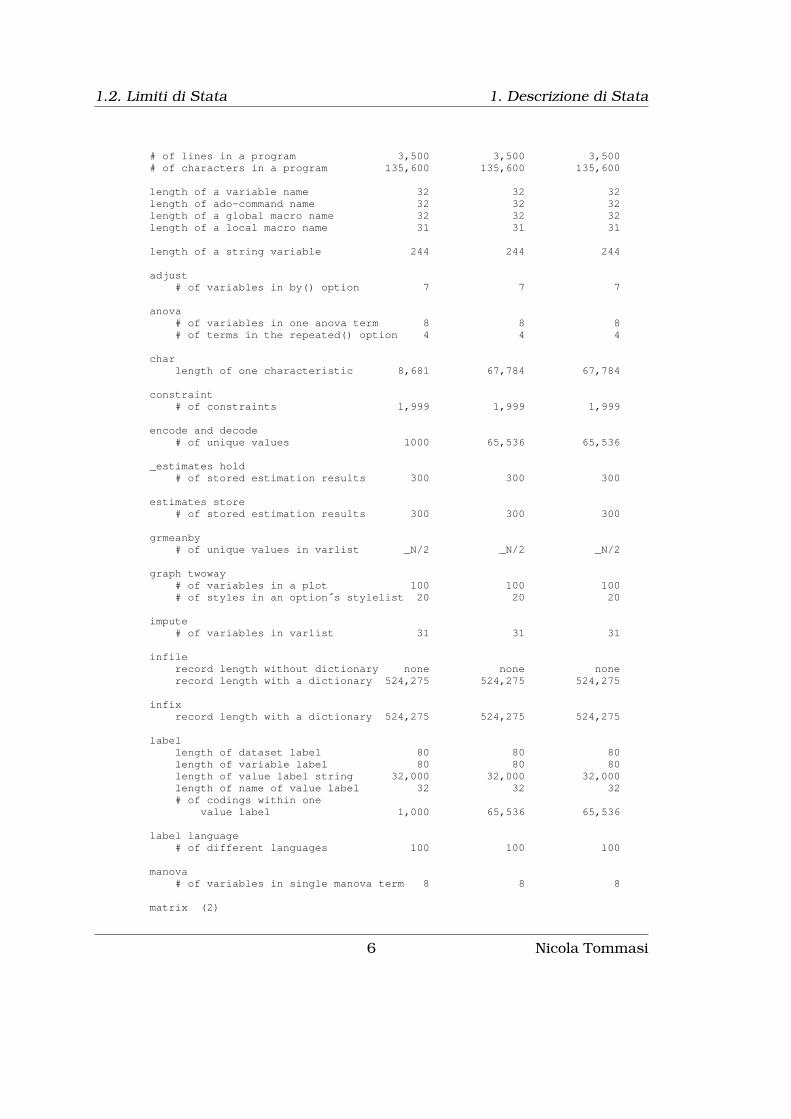
1.2. Limiti di Stata 1. Descrizione di Stata
# of lines in a program 3,500 3,500 3,500# of characters in a program 135,600 135,600 135,600
length of a variable name 32 32 32length of ado-command name 32 32 32length of a global macro name 32 32 32length of a local macro name 31 31 31
length of a string variable 244 244 244
adjust# of variables in by() option 7 7 7
anova# of variables in one anova term 8 8 8# of terms in the repeated() option 4 4 4
charlength of one characteristic 8,681 67,784 67,784
constraint# of constraints 1,999 1,999 1,999
encode and decode# of unique values 1000 65,536 65,536
_estimates hold# of stored estimation results 300 300 300
estimates store# of stored estimation results 300 300 300
grmeanby# of unique values in varlist _N/2 _N/2 _N/2
graph twoway# of variables in a plot 100 100 100# of styles in an option´s stylelist 20 20 20
impute# of variables in varlist 31 31 31
infilerecord length without dictionary none none nonerecord length with a dictionary 524,275 524,275 524,275
infixrecord length with a dictionary 524,275 524,275 524,275
labellength of dataset label 80 80 80length of variable label 80 80 80length of value label string 32,000 32,000 32,000length of name of value label 32 32 32# of codings within one
value label 1,000 65,536 65,536
label language# of different languages 100 100 100
manova# of variables in single manova term 8 8 8
matrix (2)
6 Nicola Tommasi

1. Descrizione di Stata 1.2. Limiti di Stata
dimension of single matrix 40 x 40 800 x 800 11,000x11,000
maximize optionsiterate() maximum 16,000 16,000 16,000
mlogit# of outcomes 20 50 50
net (also see usersite)# of description lines in .pkg file 100 100 100
nlogit and nlogittree# of levels in model 8 8 8
noteslength of one note 8,681 67,784 67,784# of notes attached to _dta 9,999 9,999 9,999# of notes attached to each
variable 9,999 9,999 9,999
numlist# of elements in the numeric list 1,600 1,600 1,600
ologit and oprobit# of outcomes 20 50 50
reg3, sureg, and other system estimators# of equations 40 800 11,000
set adosizememory ado-files may consume 500K 500K 500k
set scrollbufsizememory for Results window buffer 500K 500K 500k
stcox# of variables in strata() option 5 5 5
stcurve# of curves plotted on the same graph 10 10 10
table and tabdisp# of by variables 4 4 4# of margins, i.e., sum of rows,columns, supercolumns, andby groups 3,000 3,000 3,000
tabulate (3)# of rows in one-way table 500 3,000 12,000# of rows & cols in two-way table 160x20 300x20 1,200x80
tabulate, summarize (see tabsum)# of cells (rows X cols) 375 375 375
xt estimation commands (e.g., xtgee,xtgls, xtpoisson, xtprobit, xtregwith mle option, and xtpcse whenneither option hetonly nor optionindependent are specified)
# of time periods within panel 40 800 11,000# of integration points accepted 40 800 11,000by intpoints(#) 195 195 195
-----------------------------------------------------------------------------
Nicola Tommasi 7

1.2. Limiti di Stata 1. Descrizione di Stata
Notes
(1) 2,147,483,647 is a theoretical maximum; memory availability willcertainly impose a smaller maximum.
(2) In Mata, matrix is limited by the amount of memory on your computer.
(3) For Stata/IC for the Macintosh, limits are 2,000 for the number of rowsfor a one-way table and 180 for number of rows for a two-way table.
Per sapere quale versione del programma stiamo usando:
. about
Stata/SE 10.0 for WindowsBorn 25 Jul 2007Copyright (C) 1985-2007
Total physical memory: 2096624 KBAvailable physical memory: 1447220 KB
Single-user Stata for Windows perpetual license:Serial number: 81910515957
Licensed to: C.I.D.E.Univeristy of Verona
8 Nicola Tommasi
Capitolo 2
Convenzioni Tipografiche
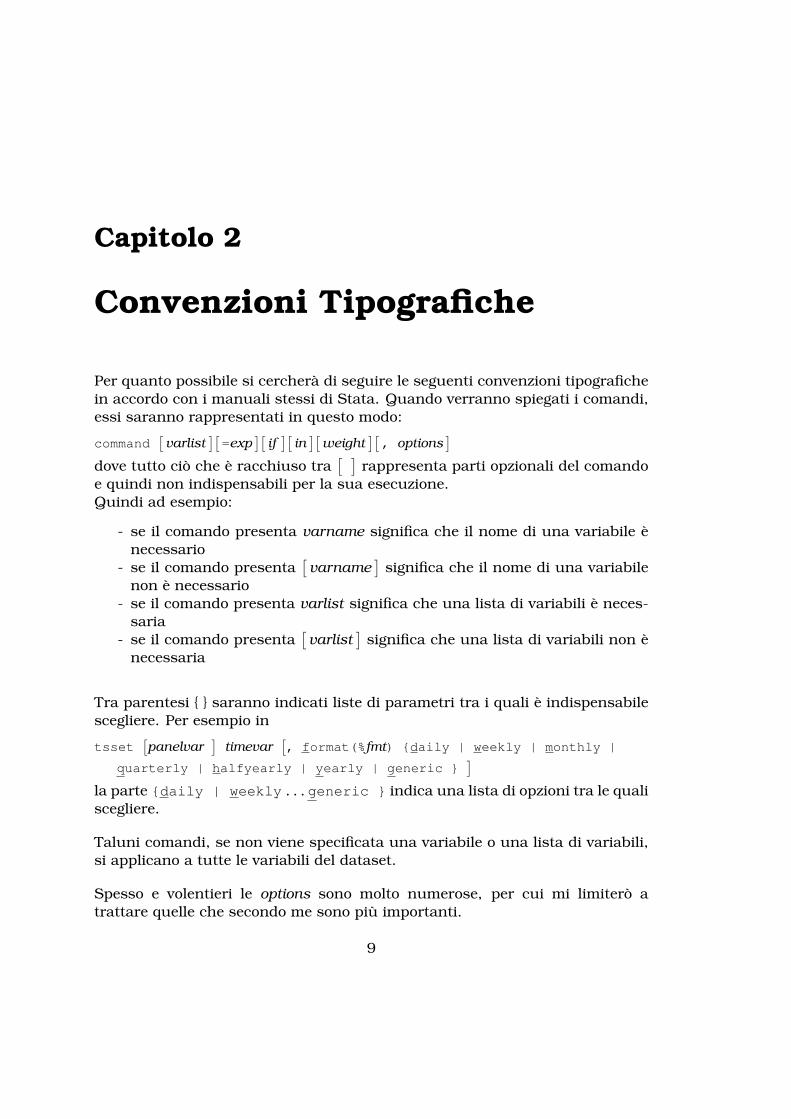
Per quanto possibile si cercherà di seguire le seguenti convenzioni tipografichein accordo con i manuali stessi di Stata. Quando verranno spiegati i comandi,essi saranno rappresentati in questo modo:
command[varlist
][=exp
][if
][in
][weight
][, options
]dove tutto ciò che è racchiuso tra
[ ]rappresenta parti opzionali del comando
e quindi non indispensabili per la sua esecuzione.Quindi ad esempio:
- se il comando presenta varname significa che il nome di una variabile ènecessario
- se il comando presenta[varname
]significa che il nome di una variabile
non è necessario- se il comando presenta varlist significa che una lista di variabili è neces-
saria- se il comando presenta
[varlist
]significa che una lista di variabili non è
necessaria
Tra parentesi { } saranno indicati liste di parametri tra i quali è indispensabilescegliere. Per esempio in
tsset[panelvar
]timevar
[, format(%fmt) {daily | weekly | monthly |
quarterly | halfyearly | yearly | generic }]
la parte {daily | weekly . . . generic } indica una lista di opzioni tra le qualiscegliere.
Taluni comandi, se non viene specificata una variabile o una lista di variabili,si applicano a tutte le variabili del dataset.
Spesso e volentieri le options sono molto numerose, per cui mi limiterò atrattare quelle che secondo me sono più importanti.
9

2. Convenzioni Tipografiche
Porzioni di files .do o output di Stata saranno indicati con il seguente layout:
. use auto(1978 Automobile Data)
. summ
Variable | Obs Mean Std. Dev. Min Max-------------+--------------------------------------------------------
make | 0price | 74 6165.257 2949.496 3291 15906
mpg | 74 21.2973 5.785503 12 41rep78 | 69 3.405797 .9899323 1 5
headroom | 74 2.993243 .8459948 1.5 5-------------+--------------------------------------------------------
trunk | 74 13.75676 4.277404 5 23weight | 74 3019.459 777.1936 1760 4840length | 74 187.9324 22.26634 142 233turn | 74 39.64865 4.399354 31 51
displacement | 74 197.2973 91.83722 79 425-------------+--------------------------------------------------------
gear_ratio | 74 3.014865 .4562871 2.19 3.89foreign | 74 .2972973 .4601885 0 1
10 Nicola Tommasi

Capitolo 3
La Filosofia del Programma
Stata è progettato per gestire efficacemente grandi quantità di dati, perciò tienetutti i dati nella memoria RAM (vedi opzione set mem)
Stata considera il trattamento dei dati come un esperimento scientifico, perciòassicura:
a. la riproducibilità tramite l’uso dei files .dob. la misurabilità tramite l’uso dei files .log o .smcl
Stata si compone di una serie di comandi che sono:
- compilati nell’eseguibile del programma- presenti in forma di file di testo con estensione .ado- scritti da terzi con la possibilità di renderli disponibili all’interno del
programma- definiti dall’utente e inseriti direttamente all’interno di files .do
Per vedere dove sono salvati i comandi scritti nei files .ado basta dare il co-mando.
. sysdirSTATA: C:\eureka\Stata10\
UPDATES: C:\eureka\Stata10\ado\updates\BASE: C:\eureka\Stata10\ado\base\SITE: C:\eureka\Stata10\ado\site\PLUS: c:\ado\stbplus\
PERSONAL: c:\ado\personal\OLDPLACE: c:\ado\
I comandi scritti da terzi solitamente si installano nella directory indicata inPLUS
Stata si usa essenzialmente da riga di comando
Gli input e gli output vengono dati in forma testuale
Di seguito si farà rifermento a variabili e osservazioni e in particolare
11

3.1. Schema di funzionamento 3. La Filosofia del Programma
ciò che in Excel viene chiamato -colonna corrisponde a variabile in Stata-riga corrisponde a osservazione in Stata
ciò che in informatica viene chiamato -campo corrisponde a variabile in Stata-record corrisponde a osservazione in Stata
3.1 Schema di funzionamento
Questo è lo schema di funzionamento del programma. Capitelo bene e saretepiù efficienti e produttivi nel vostro lavoro.
do file+--------------------------------------+| #delimit; || set more off; || clear; || set mem 150m; || capture log close; || ... || lista dei comandi da eseguire; || ... || ... || || || capture log close; || exit; |+--------------------------------------+
||--
+--------------------------------------+| || || || Stata || || ||do <do file> |+--------------------------------------+
|
12 Nicola Tommasi

3. La Filosofia del Programma 3.1. Schema di funzionamento
|-- log file
+--------------------------------------+| || || || Registrazione output comandi || del do file || || || |+--------------------------------------+
Nel do file vengono scritti in sequenza i comandi da eseguire. Questi vengonopassati al programma tramite il comando do <do_file> da impartire dallafinestra Command del programma stesso. Se non ci sono errori Stata esegueil do file e registra gli output dei comandi nel log file.
Nicola Tommasi 13


Capitolo 4
Organizzare il Lavoro
Dato che il metodo migliore di passare i comandi a Stata è la riga di comando,conviene dotarsi di un buon editor di testo. Quello integrato nel programmanon è sufficientemente potente (si possono creare al massimo file di 32k), percui consiglio di dotarsi uno dei seguenti editor gratuiti:Notepad++ -> http://notepad-plus.sourceforge.net/it/site.htmNoteTab Light -> http://www.notetab.com/PSPad -> http://www.pspad.com/RJ TextEd -> http://www.rj-texted.seTra i quatto indicati io preferisco l’ultimo. Sul sito spiegano anche comeintegrare il controllo e l’evidenziazione della sintassi dei comandi di Stata.Utilizzando editor esterni si perde la possibilità di far girare porzioni di codice;c’è però un tentativo di integrare gli editor esterni; vedi a tal proposito:http://fmwww.bc.edu/repec/bocode/t/textEditors.html
4.1 Organizzazione per cartelle di lavoro
La maniera più semplice ed efficiente di usare Stata è quella di organizzare ilproprio lavoro in directory e poi far lavorare il programma sempre all’internodi questa directory. Se si usano i percorsi relativi la posizione di tale directorydi lavoro sarà ininfluente e sarà possibile far girare i propri programmi anchesu altri computer senza dover cambiare i percorsi.In basso a sinistra, Stata mostra la directory dove attualmente sta’ puntando.In alternativa è possibile visualizzarla tramite il comando:
pwd
in questo esempio Stata punta alla cartella C:\projects\CorsoStata\esempi ese impartite il comando di esecuzione di un file .do o di caricamento di undataset senza specificare il percorso, questo verrà ricercato in questa cartella:
. pwdC:\projects\CorsoStata\esempi
15
4.1. Organizzazione per cartelle di lavoro 4. Organizzare il Lavoro
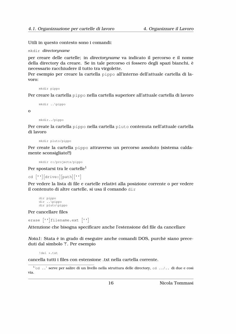
Utili in questo contesto sono i comandi:
mkdir directoryname
per creare delle cartelle; in directoryname va indicato il percorso e il nomedella directory da creare. Se in tale percorso ci fossero degli spazi bianchi, ènecessario racchiudere il tutto tra virgolette.Per esempio per creare la cartella pippo all’interno dell’attuale cartella di la-voro:
mkdir pippo
Per creare la cartella pippo nella cartella superiore all’attuale cartella di lavoro
mkdir ..\pippo
o
mkdir../pippo
Per create la cartella pippo nella cartella pluto contenuta nell’attuale cartelladi lavoro
mkdir pluto/pippo
Per create la cartella pippo attraverso un percorso assoluto (sistema calda-mente sconsigliato!!)
mkdir c:/projects/pippo
Per spostarsi tra le cartelle1
cd[''
][drive:
][path
][''
]Per vedere la lista di file e cartelle relativi alla posizione corrente o per vedereil contenuto di altre cartelle, si usa il comando dir
dir pippodir ..\pippodir pluto\pippo
Per cancellare files
erase[''
]filename.ext
[''
]Attenzione che bisogna specificare anche l’estensione del file da cancellare
Nota1: Stata è in grado di eseguire anche comandi DOS, purchè siano prece-duti dal simbolo ’!’. Per esempio
!del *.txt
cancella tutti i files con estensione .txt nella cartella corrente.
1'cd ..' serve per salire di un livello nella struttura delle directory, cd ../.. di due e cosìvia.
16 Nicola Tommasi
4. Organizzare il Lavoro 4.2. Interazione diretta VS files .do
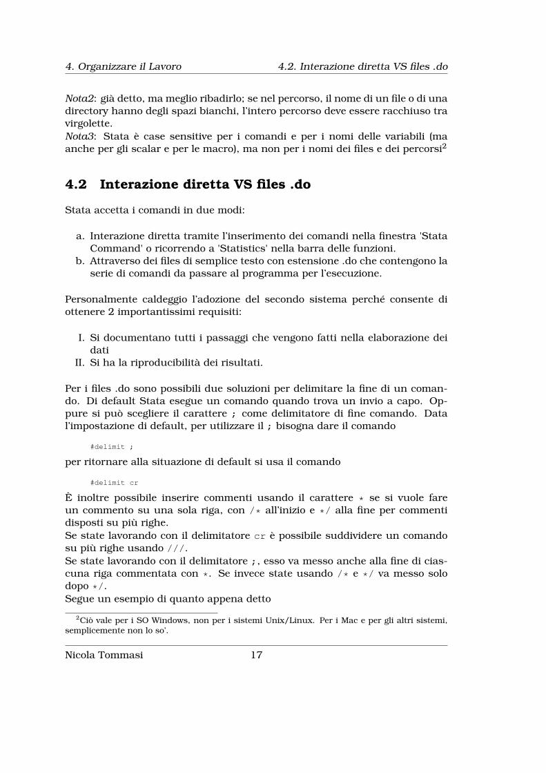
Nota2: già detto, ma meglio ribadirlo; se nel percorso, il nome di un file o di unadirectory hanno degli spazi bianchi, l’intero percorso deve essere racchiuso travirgolette.Nota3: Stata è case sensitive per i comandi e per i nomi delle variabili (maanche per gli scalar e per le macro), ma non per i nomi dei files e dei percorsi2
4.2 Interazione diretta VS files .do
Stata accetta i comandi in due modi:
a. Interazione diretta tramite l’inserimento dei comandi nella finestra 'StataCommand' o ricorrendo a 'Statistics' nella barra delle funzioni.
b. Attraverso dei files di semplice testo con estensione .do che contengono laserie di comandi da passare al programma per l’esecuzione.
Personalmente caldeggio l’adozione del secondo sistema perché consente diottenere 2 importantissimi requisiti:
I. Si documentano tutti i passaggi che vengono fatti nella elaborazione deidati
II. Si ha la riproducibilità dei risultati.
Per i files .do sono possibili due soluzioni per delimitare la fine di un coman-do. Di default Stata esegue un comando quando trova un invio a capo. Op-pure si può scegliere il carattere ; come delimitatore di fine comando. Datal’impostazione di default, per utilizzare il ; bisogna dare il comando
#delimit ;
per ritornare alla situazione di default si usa il comando
#delimit cr
È inoltre possibile inserire commenti usando il carattere * se si vuole fareun commento su una sola riga, con /* all’inizio e */ alla fine per commentidisposti su più righe.Se state lavorando con il delimitatore cr è possibile suddividere un comandosu più righe usando ///.Se state lavorando con il delimitatore ;, esso va messo anche alla fine di cias-cuna riga commentata con *. Se invece state usando /* e */ va messo solodopo */.Segue un esempio di quanto appena detto
2Ciò vale per i SO Windows, non per i sistemi Unix/Linux. Per i Mac e per gli altri sistemi,semplicemente non lo so’.
Nicola Tommasi 17

4.3. Registrazione dell'output 4. Organizzare il Lavoro
/**** #delimit cr ****/gen int y = real(substr(date,1,2))gen int m = real(substr(date,3,2))gen int d = real(substr(date,5,2))summ y m d
recode y (90=1990) (91=1991) (92=1992) (93=1993) ///(94=1994) (95=1995) (96=1996) (97=1997) (98=1998) ///(99=1999) (00=2000) (01=2001) (02=2002) ///(03=2003) (04=2004) /*serve per usare la funzione mdy*/gen new_data = mdy(m,d,y)format new_data %d
#delimit;gen int y = real(substr(date,1,2));gen int m = real(substr(date,3,2));gen int d = real(substr(date,5,2));summ y m d;
*Commento: le tre righe seguenti hanno l´invio a capo;recode y (90=1990) (91=1991) (92=1992) (93=1993)
(94=1994) (95=1995) (96=1996) (97=1997)(98=1998) (99=1999) (00=2000) (01=2001)(02=2002) (03=2003) (04=2004) /*serve per usare la funzione mdy*/;
gen new_data = mdy(m,d,y);
/******************************************questo è un commento su + righebla bla blabla bla bla*********************************************/;
format new_data %d;#delimit cr
È possibile dare l’invio a capo senza esecuzione del comando anche in modocr se si ha l’accortezza di usare i caratteri /* alla fine della riga e */ all’iniziodella successiva come mostrato nell’esempio seguente
use mydata, clearregress lnwage educ complete age age2 /*
*/ exp exp2 tenure tenure2 /**/ reg1-reg3 female
predict e, residsummarize e, detail
Attenzione: il comando #delimit non può essere usato nell’interazione direttae quindi non si possono inserire comandi nella finestra 'Command' terminandoil comando con ;
4.3 Registrazione dell'output
Stata registra gli output dell’esecuzione dei comandi in due tipi di file:
- file .smcl (tipo di default nel programma)- file .log
18 Nicola Tommasi

4. Organizzare il Lavoro 4.4. Aggiornare il programma
I files .smcl sono in formato proprietario di Stata e “abbelliscono” l’outputcon formattazioni di vario tipo (colori, grassetto, corsivo...), ma possono esserevisualizzati solo con l’apposito editor integrato nel programma3.I files .log sono dei semplici file di testo senza nessun tipo di formattazione epossono essere visualizzati con qualsiasi editor di testo.Si può scegliere il tipo di log attraverso il comando
set logtype text|smcl[, permanently
]Si indica al programma di iniziare la registrazione tramite il comando
log using filename[, append replace
[text|smcl
]name(logname)
]La registrazione può essere sospesa tramite:
log off[logname
]ripresa con
log on[logname
]e infine chiusa con
log close[logname
]A partire dalla versione 10 è possibile aprire più files di log contemporanea-mente.
4.4 Aggiornare il programma
Il corpo principale del programma di aggiorna tramite il comando
update all
. update all
----------------------------------------------------> update ado(contacting http://www.stata.com)ado-files already up to date
----------------------------------------------------> update executable(contacting http://www.stata.com)executable already up to date
in questo modo verranno prima aggiornati i files .ado di base del program-ma e poi l’eseguibile .exe. In quest’ultimo caso verrà richiesto il riavvio delprogramma.Se non si possiede una connessione ad internet, sul sito di Stata è possibilescaricare gli archivi compressi degli aggiornamenti da installare all’indirizzohttp://www.stata.com/support/updates/
3Attraverso 'File -> Log -> View' o apposita icona.
Nicola Tommasi 19

4.5. Aggiungere comandi 4. Organizzare il Lavoro
Sul sito vengono fornite tutte le istruzioni per portare a termine questa proce-dura
4.5 Aggiungere comandi
Come accennato in precedenza è possibile aggiungere nuovi comandi scritti daterze parti. Per fare ciò è necessario conoscere il nome del nuovo comando edare il comando
ssc install pkgname[, all replace
]. ssc inst bitobitchecking bitobit consistency and verifying not already installed...installing into c:\ado\plus\...installation complete.
Di recente ad ssc è stata aggiunta la possibilità di vedere i comandi aggiuntivi(packages) più scaricati negli ultimi tre mesi:
ssc whatshot[, n(#)
]dove # specifica il numero di packages da visualizzare (n(10) è il valore didefault). Specificando n(.) verrà visualizzato l’intero elenco.
. ssc whatshot, n(12)
Top 12 packages at SSC
Oct2007Rank # hits Package Author(s)----------------------------------------------------------------------
1 1214.0 outreg John Luke Gallup2 911.1 estout Ben Jann3 847.6 xtabond2 David Roodman4 830.8 outreg2 Roy Wada5 788.6 ivreg2 Mark E Schaffer, Christopher F Baum,
Steven Stillman6 667.8 psmatch2 Edwin Leuven, Barbara Sianesi7 508.2 gllamm Sophia Rabe-Hesketh8 320.3 xtivreg2 Mark E Schaffer9 315.3 overid Christopher F Baum, Mark E Schaffer,
Steven Stillman, Vince Wiggins10 266.0 tabout Ian Watson11 251.0 ranktest Mark E Schaffer, Frank Kleibergen12 246.4 metan Mike Bradburn, Ross Harris, Jonathan
Sterne, Doug Altman, Roger Harbord,Thomas Steichen, Jon Deeks
----------------------------------------------------------------------(Click on package name for description)
Siete curiosi di vedere tutti i pacchetti disponibili? Andate in Appendice B(pag. 255).Esiste anche la possibilità di installare i nuovi comandi attraverso la fun-zione di ricerca. In questo caso vengono fornite direttamente le indicazionida seguire4.
4In pratica la procedura vi dirà cosa cliccare per procedere automaticamente all’installazione.
20 Nicola Tommasi

4. Organizzare il Lavoro 4.6. Fare ricerche
Non è raro (anzi) che questi nuovi comandi vengano corretti per dei bugs, op-pure migliorati con l’aggiunta di nuove funzioni. Per controllare gli update ditutti i nuovi comandi installati si usa il comando
adoupdate[pkglist
][, options
]. adoupdate, update(note: adoupdate updates user-written files;
type -update- to check for updates to official Stata)
Checking status of installed packages...
[1] mmerge at http://fmwww.bc.edu/repec/bocode/m:installed package is up to date
[2] sg12 at http://www.stata.com/stb/stb10:installed package is up to date
(output omitted )
[96] sjlatex at http://www.stata-journal.com/production:installed package is up to date
[97] hotdeck at http://fmwww.bc.edu/repec/bocode/h:installed package is up to date
Packages to be updated are...
[90] examples -- ´EXAMPLES´: module to show examples from on-line help files
Installing updates...
[90] examples
Cleaning up... Done
il quale si occupa del controllo delle nuove versioni e quindi della loro instal-lazione.
4.6 Fare ricerche
Stata dispone di 2 comandi per cercare informazioni e di un comando perottenere l’help dei comandiPer ottenere l’help basta digitare :
help[command_or_topic_name
][, options
]Per fare ricerche si possono usare indifferentemente:
search word[word ...
][, search_options
]oppure
findit word[word ...
]Personalmente preferisco il secondo. Entrambi i comandi effettuano una ricer-ca sui comandi e sulla documentazione locale e su tutte le risorse di Statadisponibili in rete.
Nicola Tommasi 21
4.6. Fare ricerche 4. Organizzare il Lavoro
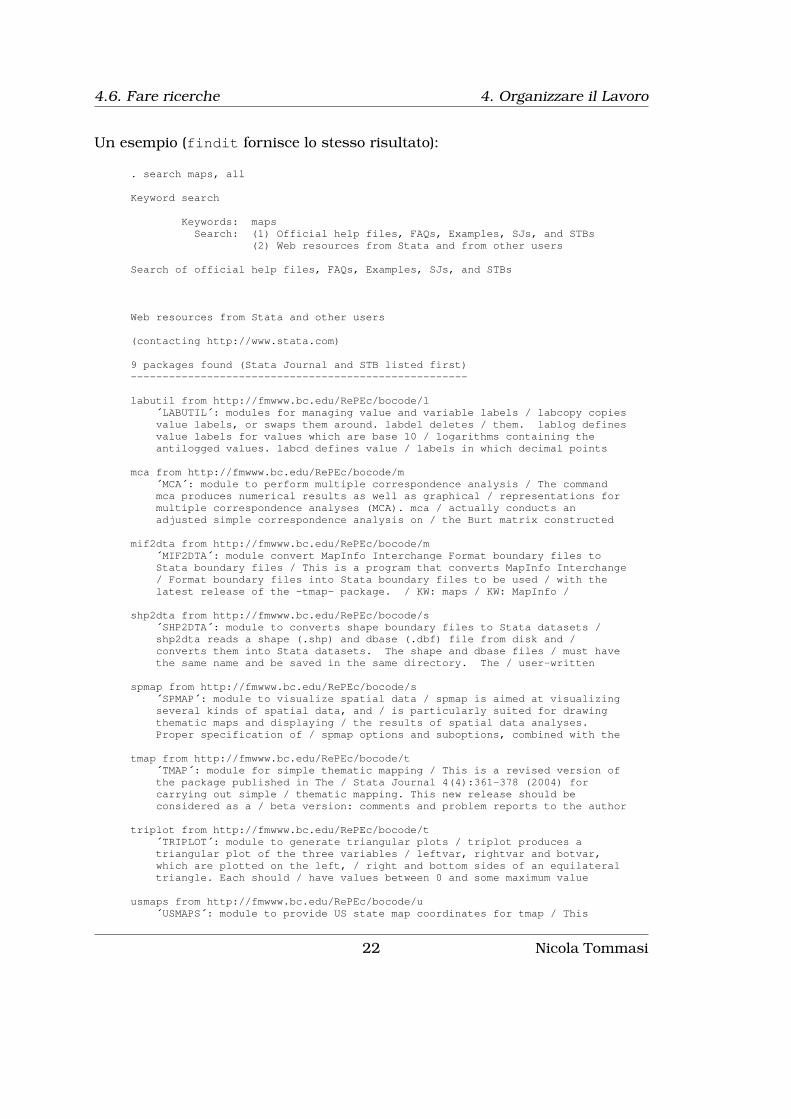
Un esempio (findit fornisce lo stesso risultato):
. search maps, all
Keyword search
Keywords: mapsSearch: (1) Official help files, FAQs, Examples, SJs, and STBs
(2) Web resources from Stata and from other users
Search of official help files, FAQs, Examples, SJs, and STBs
Web resources from Stata and other users
(contacting http://www.stata.com)
9 packages found (Stata Journal and STB listed first)-----------------------------------------------------
labutil from http://fmwww.bc.edu/RePEc/bocode/l´LABUTIL´: modules for managing value and variable labels / labcopy copiesvalue labels, or swaps them around. labdel deletes / them. lablog definesvalue labels for values which are base 10 / logarithms containing theantilogged values. labcd defines value / labels in which decimal points
mca from http://fmwww.bc.edu/RePEc/bocode/m´MCA´: module to perform multiple correspondence analysis / The commandmca produces numerical results as well as graphical / representations formultiple correspondence analyses (MCA). mca / actually conducts anadjusted simple correspondence analysis on / the Burt matrix constructed
mif2dta from http://fmwww.bc.edu/RePEc/bocode/m´MIF2DTA´: module convert MapInfo Interchange Format boundary files toStata boundary files / This is a program that converts MapInfo Interchange/ Format boundary files into Stata boundary files to be used / with thelatest release of the -tmap- package. / KW: maps / KW: MapInfo /
shp2dta from http://fmwww.bc.edu/RePEc/bocode/s´SHP2DTA´: module to converts shape boundary files to Stata datasets /shp2dta reads a shape (.shp) and dbase (.dbf) file from disk and /converts them into Stata datasets. The shape and dbase files / must havethe same name and be saved in the same directory. The / user-written
spmap from http://fmwww.bc.edu/RePEc/bocode/s´SPMAP´: module to visualize spatial data / spmap is aimed at visualizingseveral kinds of spatial data, and / is particularly suited for drawingthematic maps and displaying / the results of spatial data analyses.Proper specification of / spmap options and suboptions, combined with the
tmap from http://fmwww.bc.edu/RePEc/bocode/t´TMAP´: module for simple thematic mapping / This is a revised version ofthe package published in The / Stata Journal 4(4):361-378 (2004) forcarrying out simple / thematic mapping. This new release should beconsidered as a / beta version: comments and problem reports to the author
triplot from http://fmwww.bc.edu/RePEc/bocode/t´TRIPLOT´: module to generate triangular plots / triplot produces atriangular plot of the three variables / leftvar, rightvar and botvar,which are plotted on the left, / right and bottom sides of an equilateraltriangle. Each should / have values between 0 and some maximum value
usmaps from http://fmwww.bc.edu/RePEc/bocode/u´USMAPS´: module to provide US state map coordinates for tmap / This
22 Nicola Tommasi
4. Organizzare il Lavoro 4.7. Cura dei dati
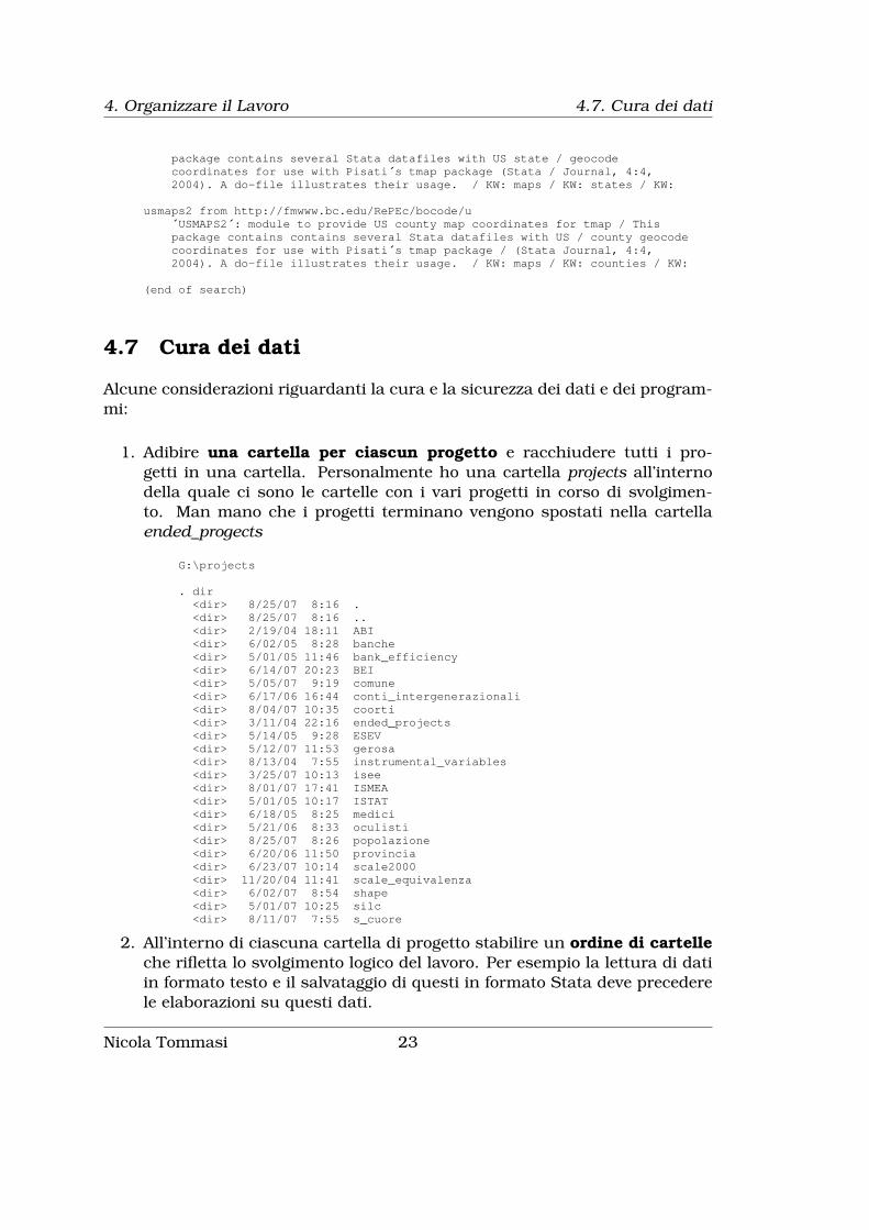
package contains several Stata datafiles with US state / geocodecoordinates for use with Pisati´s tmap package (Stata / Journal, 4:4,2004). A do-file illustrates their usage. / KW: maps / KW: states / KW:
usmaps2 from http://fmwww.bc.edu/RePEc/bocode/u´USMAPS2´: module to provide US county map coordinates for tmap / Thispackage contains contains several Stata datafiles with US / county geocodecoordinates for use with Pisati´s tmap package / (Stata Journal, 4:4,2004). A do-file illustrates their usage. / KW: maps / KW: counties / KW:
(end of search)
4.7 Cura dei dati
Alcune considerazioni riguardanti la cura e la sicurezza dei dati e dei program-mi:
1. Adibire una cartella per ciascun progetto e racchiudere tutti i pro-getti in una cartella. Personalmente ho una cartella projects all’internodella quale ci sono le cartelle con i vari progetti in corso di svolgimen-to. Man mano che i progetti terminano vengono spostati nella cartellaended_progects
G:\projects
. dir<dir> 8/25/07 8:16 .<dir> 8/25/07 8:16 ..<dir> 2/19/04 18:11 ABI<dir> 6/02/05 8:28 banche<dir> 5/01/05 11:46 bank_efficiency<dir> 6/14/07 20:23 BEI<dir> 5/05/07 9:19 comune<dir> 6/17/06 16:44 conti_intergenerazionali<dir> 8/04/07 10:35 coorti<dir> 3/11/04 22:16 ended_projects<dir> 5/14/05 9:28 ESEV<dir> 5/12/07 11:53 gerosa<dir> 8/13/04 7:55 instrumental_variables<dir> 3/25/07 10:13 isee<dir> 8/01/07 17:41 ISMEA<dir> 5/01/05 10:17 ISTAT<dir> 6/18/05 8:25 medici<dir> 5/21/06 8:33 oculisti<dir> 8/25/07 8:26 popolazione<dir> 6/20/06 11:50 provincia<dir> 6/23/07 10:14 scale2000<dir> 11/20/04 11:41 scale_equivalenza<dir> 6/02/07 8:54 shape<dir> 5/01/07 10:25 silc<dir> 8/11/07 7:55 s_cuore
2. All’interno di ciascuna cartella di progetto stabilire un ordine di cartelleche rifletta lo svolgimento logico del lavoro. Per esempio la lettura di datiin formato testo e il salvataggio di questi in formato Stata deve precederele elaborazioni su questi dati.
Nicola Tommasi 23

4.7. Cura dei dati 4. Organizzare il Lavoro
. cd conti_intergenerazionaliG:\projects\conti_intergenerazionali
. dir<dir> 6/17/06 16:44 .<dir> 6/17/06 16:44 ..<dir> 6/24/06 15:52 00_docs<dir> 4/25/06 8:18 01_original_data<dir> 6/02/06 9:29 02_final_data<dir> 6/02/06 9:29 03_source<dir> 6/02/06 9:29 04_separazioni<dir> 6/04/06 11:39 05_disoccupazione<dir> 6/02/06 9:29 06_povertà<dir> 6/25/06 9:13 99_GA0.5k 8/30/05 8:50 master.do
3. Ci dovrebbe sempre essere un file master.do che si occupa di lanciaretutti i files .do nell’ordine corretto.master.do di conti_intergenerazionali
#delimit;clear;set mem 250m;set more off;capture log close;cd 02_final_data;do read.do /** che lancia, nell´ordine -panel_link.do
-panel_a.do-panel_h.do
****/;cd ..;
cd 03_source;do master.do;cd ..;
cd 04_separazioni;do master.do;cd ..;
cd 05_disoccupazione;do master.do;cd ..;
cd 99_GA;do master.do;cd ..;
master.do di 03_source
clear
do rela.dodo coppie.dodo rela_by_wave.dodo hids.dodo sons.dodo occupati.do
4. Usare sempre percorsi relativi.5. I files di dati di partenza devono rimanere inalterati. Se i dati di partenza
vengono in qualsiasi modo modificati vanno salvati con un altro nome.
24 Nicola Tommasi

4. Organizzare il Lavoro 4.8. Intestazione file .do
Altrimenti si inficia il principio di riproducibilità6. Dare ai files di log lo stesso nome del file do che li genera.7. Fare un backup giornaliero dei propri progetti (sia files di dati che files
.do). Un backup fatto male (o non fatto) può far piangere anche un uomogrande e grosso.
8. I dati sensibili vanno protetti. Si possono separare gli identificativi per-sonali dal resto dei dati e poi i files con questi dati andrebbero criptati.
4.8 Intestazione file .do
Naturalmente questa è solo un’indicazione per nulla vincolante; ciascuno fac-cia come meglio crede, ma io consiglio di iniziare i files .do così:
#delimit;clear;set mem 250m;set more off;capture log close;log using panel.log, replace;
Cosa faccio con questo incipit?
#delimit; definisco il delimitatore di fine comandoclear; elimino eventuali dati in memoriaset mem 250m; assegno un adeguato quantitativo di memoriaset more off; disabilito lo stop nello scorrimento qualora l’output di un co-
mando ecceda la lunghezza della schermata della finestra dei risultati delprogramma
capture log close; chiudo un eventuale file di log apertolog using xxxxxx.log, replace; avvio la registrazione degli output. Con
replace sovrascrivo un eventuale file di log con lo stesso nome. Possibil-mente assegnare al file xxxxxx.log lo stesso nome del file .do.
P.S.: Il nome del file .do dovrebbe essere breve (non più di otto lettere diciamo)e non contenere spazi bianchi.
Nicola Tommasi 25


Capitolo 5
Alcuni Concetti di Base
5.1 L’input dei dati
5.1.1 Caricamento dei dati in formato proprietario
Vale la regola generale che la realise più recente legge i dati scritti nelle realiseprecedenti, ma le precedenti non leggono quelle più recenti. Inoltre bisognatener presente anche la versione del programma secondo il presente schemahhhhhhhhhhhhhhhhhhDati salvati da
Dati letti daStataMP StataSE Intercooled Small
StataMP SI SI NO NOStataSE SI SI NO NOIntercooled SI SI SI SI(?)Small SI SI SI SI
Il comando per caricare i dati in formato proprietario di Stata (estensione .dta)è
use filename[, clear
]L’opzione clear è necessaria per pulire la memoria dall’eventuale presenza dialtri dati, in quanto non ci possono essere 2 database contemporaneamentein memoria. Questo argomento viene trattato in forma maggiormente estesa edettagliata nel capitolo 6.1 alla pagina 37.
5.1.2 Caricamento dei dati in formato testo
Esistono diversi comandi in Stata per caricare dati in formato testo (ASCII).Val la pena di ricordare che questo formato sarebbe da preferire quando i datisaranno utilizzati anche con altri programmi1.
1I dati in formato testo sono leggeri in termini di dimensione del file, molto raramente sidanneggiano e sono utilizzabili anche su piattaforme diverse da quelle Microsoft.
27

5.2. Regole per denominare le variabili 5. Alcuni Concetti di Base
La prima cosa da sapere è se i dati sono delimitati o non delimitati. I dati sonodelimitati se ciascuna variabile è separata da un certo carattere, di solito
- '.'- ',' 2
- ';'- '|'- '<tab>'
Qui viene fatta solo un’introduzione ai dati in formato testo. La trattazione peresteso verrà fatta nel capitolo 6.2 alla pagina 41.
5.1.3 Caricamento dei dati in altri formati proprietari (StatTrans-fer)
È possibile convertire dataset da altri formati al formato di Stata attraversoil programma commerciale StatTransfer, consigliato dalla stessa Stata Corp.Questo programma è usabile anche direttamente all’interno di Stata tramiteappositi comandi che vedremo più avanti (inputst e outputst) nel capitolo 6.3alla pagina 45.
5.2 Regole per denominare le variabili
Esistono due metodi per nominare le variabili: assegnare un nome evocati-vo o assegnare un codice. Per esempio possiamo chiamare redd la variabileche contiene l’informazione sul reddito o age la variabile che contiene l’infor-mazione sull’età. In questa maniera il nome della variabile ci aiuta a richiamareil suo contenuto informativo. Se però abbiamo centinaia di variabili, assegnarea ciascuna un nome evocativo può diventare problematico. In questo contestomeglio ricorrere ad una nomenclatura di tipo sistematico. Per esempio asseg-nare d01 d02 d03 d04 d05 alle risposte delle domande da 1 a 5 o nomi deltipo score_10 score_11 ... o ancora 14a_rc d14b_rc d14c_rc d14d_rcd14e_rc d14f_rc.Quelle che seguono sono regole (e consigli) cui sono sottoposti i nomi cheintendiamo assegnare alle variabili:
1. Ogni variabile deve avere il suo nome2. Il nome di ciascuna variabile deve essere univoco3. Il nome delle variabili è case sensitive per cui redd è diverso da REDD o da
Redd4. Il nome non deve contenere2I caratteri '.' e ',' non sono consigliati in quanto possono generare confusione in relazione
alla sintassi numerica europea e anglosassone.
28 Nicola Tommasi

5. Alcuni Concetti di Base 5.3. Il qualificatore in
(a) spazi(b) trattini (-). è invece consentito l’underscore (_)(c) caratteri non alfabetici o non numerici ( . , ; : C # § * ^ ? ’ = )
( [ ] / \ & % $ £ ” ! | > <)
5. Il nome non può iniziare con un numero6. La lunghezza non può superare i 32 caratteri anche se per motivi di
praticità è consigliabile non superare la decina di caratteri7. Possibilmente usare solo lettere minuscole (sempre per motivi di praticità)8. Meglio non usare lettere accentate
5.3 Il qualificatore in
Buona parte dei comandi di Stata supportano l’uso del qualificatore in che,assieme al qualificatore if, consente di restringere l’insieme delle osservazionisu cui applicare il comando. Si noti che questo qualificatore risente dell’ordina-mento dei dati, nel senso che fa riferimento alla posizione assoluta dell’osser-vazione. Un piccolo esempio può aiutare la comprensione di questo concetto.Supponiamo di avere 10 osservazioni per 2 variabili come segue:
sex age1. 1 452. 2 223. 1 114. 1 365. 2 886. 1 477. 2 728. 2 189. 2 17
se eseguo i seguenti comandi
. list sex age in 2/6
+-----------+| sex age ||-----------|
2. | 2 22 |3. | 1 11 |4. | 1 36 |5. | 2 88 |6. | 1 47 |
+-----------+
. summ age in 2/6
Variable | Obs Mean Std. Dev. Min Max-------------+--------------------------------------------------------
age | 5 40.8 29.71027 11 88
Stata mostra le osservazione dalla 2. alla 6. ed esegue il comando summ sulleosservazioni 2.-6.Se adesso ordino le il dataset in base alla variabile age
Nicola Tommasi 29

5.4. Il qualificatore if 5. Alcuni Concetti di Base
. sort age
. list
+-----------+| sex age ||-----------|
1. | 1 11 |2. | 2 17 |3. | 2 18 |4. | 2 22 |5. | 1 36 |
|-----------|6. | 1 45 |7. | 1 47 |8. | 2 72 |9. | 2 88 |
+-----------+
e rieseguo gli stessi comandi
. list sex age in 2/6
+-----------+| sex age ||-----------|
2. | 2 17 |3. | 2 18 |4. | 2 22 |5. | 1 36 |6. | 1 45 |
+-----------+
. summ age in 2/6
Variable | Obs Mean Std. Dev. Min Max-------------+--------------------------------------------------------
age | 5 27.6 12.34099 17 45
Stata mostra ancora le osservazione dalla 2. alla 6. ed esegue il comandosumm sulle osservazioni 2.-6. ma con risultati differenti perchè il comandosort ha cambiato la posizione delle osservazioni. Da questo esempio si evi-denzia che va posta attenzione nell’uso del qualificatore in in quanto il coman-do associato non viene sempre applicato alle stesse osservazioni, ma dipendedall’ordinamento delle osservazioni (sort)
5.4 Il qualificatore if
La quasi totalità dei comandi di Stata supporta l’uso del qualificatore if. Es-so ha la funzione di selezionare le osservazioni su cui applicare il comandovincolando la scelta al verificarsi della condizione specificata nell’ if. Anche inquesto caso un esempio aiuta la comprensione. Sempre facendo riferimento aldataset appena usato:
. list sex age if sex==1
30 Nicola Tommasi
5. Alcuni Concetti di Base 5.5. Operatori di relazione
+-----------+| sex age ||-----------|
1. | 1 11 |5. | 1 36 |6. | 1 45 |7. | 1 47 |
+-----------+
. summ sex age if sex==1
Variable | Obs Mean Std. Dev. Min Max-------------+--------------------------------------------------------
sex | 4 1 0 1 1age | 4 34.75 16.54035 11 47
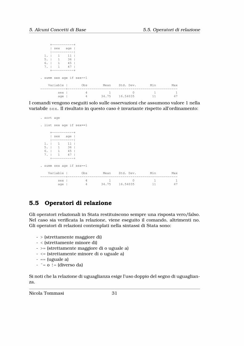
I comandi vengono eseguiti solo sulle osservazioni che assumono valore 1 nellavariabile sex. Il risultato in questo caso è invariante rispetto all’ordinamento:
. sort age
. list sex age if sex==1
+-----------+| sex age ||-----------|
1. | 1 11 |5. | 1 36 |6. | 1 45 |7. | 1 47 |
+-----------+
. summ sex age if sex==1
Variable | Obs Mean Std. Dev. Min Max-------------+--------------------------------------------------------
sex | 4 1 0 1 1age | 4 34.75 16.54035 11 47
5.5 Operatori di relazione
Gli operatori relazionali in Stata restituiscono sempre una risposta vero/falso.Nel caso sia verificata la relazione, viene eseguito il comando, altrimenti no.Gli operatori di relazioni contemplati nella sintassi di Stata sono:
- > (strettamente maggiore di)- < (strettamente minore di)- >= (strettamente maggiore di o uguale a)- <= (strettamente minore di o uguale a)- == (uguale a)- ˜= o != (diverso da)
Si noti che la relazione di uguaglianza esige l’uso doppio del segno di uguaglian-za.
Nicola Tommasi 31
5.6. Operatori logici 5. Alcuni Concetti di Base
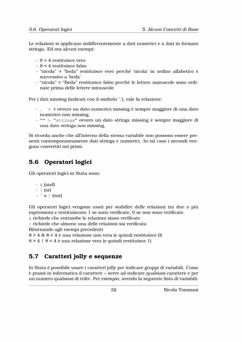
Le relazioni si applicano indifferentemente a dati numerici e a dati in formatostringa. Ed ora alcuni esempi:
- 8 > 4 restituisce vero- 8 < 4 restituisce falso- “nicola” > “beda” restituisce vero perché 'nicola' in ordine alfabetico è
successivo a 'beda'- “nicola” > “Beda” restituisce falso perché le lettere maiuscole sono ordi-
nate prima delle lettere minuscole
Per i dati missing (indicati con il simbolo '.'), vale la relazione:
- . > # ovvero un dato numerico missing è sempre maggiore di una datonumerico non missing.
- “” > “stringa” ovvero un dato stringa missing è sempre maggiore diuna dato stringa non missing.
Si ricorda anche che all’interno della stessa variabile non possono essere pre-senti contemporaneamente dati stringa e numerici. In tal caso i secondi ven-gono convertiti nei primi.
5.6 Operatori logici
Gli operatori logici in Stata sono:
- & (and)- | (or)- ˜ o ! (not)
Gli operatori logici vengono usati per stabilire delle relazioni tra due o piùespressioni e restituiscono 1 se sono verificate, 0 se non sono verificate.& richiede che entrambe le relazioni siano verificate| richiede che almeno una delle relazioni sia verificataRitornando agli esempi precedenti8 > 4 & 8 < 4 è una relazione non vera (e quindi restituisce 0)8 > 4 | 8 < 4 è una relazione vera (e quindi restituisce 1)
5.7 Caratteri jolly e sequenze
In Stata è possibile usare i caratteri jolly per indicare gruppi di variabili. Comeè prassi in informatica il carattere * serve ad indicare qualsiasi carattere e perun numero qualsiasi di volte. Per esempio, avendo la seguente lista di variabili:
32 Nicola Tommasi

5. Alcuni Concetti di Base 5.8. L’espressione by
redd95spesa1995redd96spesa1996redd97spesa1997redd1998ageriscsesso
- * indica tutte le variabili- *95 indica redd95 e spesa95- r* indica redd95, redd96, redd97 e risc
Il carattere ? invece serve per indicare un qualsiasi carattere per una solavolta; nel nostro esempio:
- ? indica nessuna variabile perché non c’è nessuna variabile di un solocarattere, qualsiasi esso sia
- ????95 indica solo redd95, ma non spesa95 (solo 4 caratteri prima di 95)- redd?? indica redd95, redd96, redd97 ma non redd1998 (solo 2 carat-
teri dopo redd)
Con il simbolo - si indica una successione contigua di variabili; sempre nelnostro caso,redd96-risc indica redd96, spesa1996, redd97, spesa1997, redd1998, age,risc.
Si faccia attenzione che il simbolo - dipende da come sono disposte le variabili.Se la variabile redd97 venisse spostata all’inizio della lista, non rientrerebbepiù nell’elenco.
5.8 L’espressione by
Molti comandi hanno la caratteristica di essere byable, ovvero supportano l’usodel prefisso by. In sostanza il by serve per ripetere un comando più volte inbase ad una certa variabile (categorica). Supponiamo di avere l’età (age) di Nindividui e di sapere per ciascuno di essi se risiede nelle macro regioni nord,centro o sud+isole (macro3). Volendo conoscere l’età media per ciascuna dellemacro regioni (nord=1, centro=2, sud+isole=3):
. summ age if macro3==1
Variable | Obs Mean Std. Dev. Min Max-------------+--------------------------------------------------------
age | 12251 55.90948 15.82015 19 101
Nicola Tommasi 33

5.9. Dati missing 5. Alcuni Concetti di Base
. summ age if macro3==2
Variable | Obs Mean Std. Dev. Min Max-------------+--------------------------------------------------------
age | 5253 56.56958 16.03001 19 98
. summ age if macro3==3
Variable | Obs Mean Std. Dev. Min Max-------------+--------------------------------------------------------
age | 9995 55.96738 15.69984 21 102
oppure, ricorrendo al by e all’uso di una sola riga di comando al posto delle 3precedenti:
. by macro3, sort: summ age
-----------------------------------------------------------------------> macro3 = Nord
Variable | Obs Mean Std. Dev. Min Max-------------+--------------------------------------------------------
age | 12251 55.90948 15.82015 19 101
-----------------------------------------------------------------------> macro3 = Centro
Variable | Obs Mean Std. Dev. Min Max-------------+--------------------------------------------------------
age | 5253 56.56958 16.03001 19 98
-----------------------------------------------------------------------> macro3 = Sud & Isole
Variable | Obs Mean Std. Dev. Min Max-------------+--------------------------------------------------------
age | 9995 55.96738 15.69984 21 102
Per l’esecuzione tramite by bisogna che il dataset sia preventivamente ordinatoin base alla variabile categorica, da cui l’uso dell’opzione sort. Alternativa-mente si può ricorrere alla variazione di questo comando:
bysort macro3: summ age
che da’ il medesimo risultato del precedente.Vedremo in seguito che by rientra anche tra le opzioni di molti comandi, percui esso può assumere la duplice natura di prefisso e di opzione.
5.9 Dati missing
Stata identifica con il simbolo '.' un dato missing numerico. Questa è la suarappresentazione generale ma c’è la posibilità di definire un sistema di identi-ficazione di valori missing di diversa natura. Per esempio un dato missing permancata risposta è concettualmente diverso da un dato missing dovuto al fattoche quella domanda non può essere posta. Un dato missing sull’occupazionedi un neonato non è una mancata risposta ma una domanda che non può es-
34 Nicola Tommasi

5. Alcuni Concetti di Base 5.9. Dati missing
sere posta. In Stata possiamo definire diversi missing secondo la struttura .a,.b, .c, ... .z e vale l’ordinamento:
tutti i numeri non missing < . < .a < .b < ... < .z
Poi a ciascuno di questi diversi missing possiamo assegnare una sua label:
label define 1 "......"2 "......".............a "Non risponde".b "Non sa".c "Non appicabile"
Quanto esposto precedentemente si riferisce a dati numerici. Per le variabilistringa non esiste nessun metodo di codifica e il dato missing corrisponde aduna cella vuota (nessun simbolo e nessuno spazio). Nel caso si debba fareriferimento ad un dato missing stringa si usano le doppie vigolette come segue:
. desc q01 q03
storage display valuevariable name type format label variable label----------------------------------------------------------------------q01 int %8.0g q01 etàq03 str29 %29s q03 comune di residenza
. summ q01 if q03==""
Variable | Obs Mean Std. Dev. Min Max-------------+--------------------------------------------------------
q01 | 12 49.75 29.19877 1 90
Nicola Tommasi 35


Capitolo 6
Il Caricamento dei Dati
6.1 Dati in formato proprietario (.dta)
Caricare i dati in formato Stata (.dta) è un’operazione semplice e come ve-dremo ci sono diverse utili opzioni. Ma prima di caricare un dataset bisognaporre attenzione alla sua dimensione. Come già accennato Stata mantiene tuttii dati nella memoria RAM per cui bisogna allocarne un quantitativo adegua-to, il quale, sarà sottratto alla memoria di sistema. Se per esempio dobbiamocaricare un file di dati di 88MB dobbiamo dedicare al programma questo quan-titativo aumentato in funzione della eventuale creazione di nuove variabili. Sepossibile consiglio di allocare un quantitativo di RAM all’incirca doppio rispettoal dataset di partenza se si dovranno creare molte nuove variabili, altrimentiun incremento del 50% può essere sufficiente dato che un certo quantitativodi RAM viene comunque utilizzato per le elaborazioni. Stata è impostato conuna allocazione di default di circa 1.5MB.Nel momento in cui avviate il programma vi viene fornita l’informazione circal’attuale allocazione di RAM.
Notes:1. (/m# option or -set memory-) 10.00 MB allocated to data2. (/v# option or -set maxvar-) 5000 maximum variables
Il comando per allocare un diverso quantitativo di memoria è :
set memory #[b|k|m|g
][, permanently
]. set mem 250m
Current memory allocation
current memory usagesettable value description (1M = 1024k)--------------------------------------------------------------------set maxvar 5000 max. variables allowed 1.909Mset memory 250M max. data space 250.000Mset matsize 400 max. RHS vars in models 1.254M
-----------
37

6.1. Dati in formato proprietario (.dta) 6. Il Caricamento dei Dati
253.163M
e va eseguito prima di caricare il dataset, ovvero con nessun dataset in memo-ria1.Inoltre bisogna tener presenti le seguenti limitazioni:
- il quantitativo di RAM dedicato non deve superare la RAM totale delcomputer e tenete presente che un certo quantitativo serve anche peril normale funzionamento del sistema operativo.
- attualmente Windows ha problemi ad allocare quantitativi superiori ai950MB2.
Se volete allocare in maniera permanente un certo quantitativo di RAM inmaniera che ad ogni avvio questo sia a disposizione di Stata:
set mem #m, perm
Se il quantitativo di memoria non è sufficiente, Stata non carica i dati:
. use istat03, clear(Indagine sui Consumi delle Famiglie - Anno 2003)no room to add more observations
An attempt was made to increase the number of observations beyond what iscurrently possible.You have the following alternatives:
1. Store your variables more efficiently; see help compress.(Think of Stata´s data area as the area of a rectangle; Stata can tradeoff width and length.)
2. Drop some variables or observations; see help drop.
3. Increase the amount of memory allocated to the data area using the setmemory command; see help memory.
r(901);
. set mem 5m
Current memory allocation
current memory usagesettable value description (1M = 1024k)--------------------------------------------------------------------set maxvar 5000 max. variables allowed 1.909Mset memory 5M max. data space 5.000Mset matsize 400 max. RHS vars in models 1.254M
-----------8.163M
. use istat03, clear(Indagine sui Consumi delle Famiglie - Anno 2003)
. desc, short
Contains data from istat03.dta
1Ricordo che ci può essere un solo dataset in memoria.2Il problema per la versione italiana dovrebbe essere risolto con il prossimo rilascio del service
pack 3 di Windows XP.
38 Nicola Tommasi

6. Il Caricamento dei Dati 6.1. Dati in formato proprietario (.dta)
obs: 2,000 Indagine sui Consumi delleFamiglie - Anno 2003
vars: 551 23 Nov 2006 09:13size: 2,800,000 (46.6% of memory free)Sorted by:
Allocato un quantitativo adeguato di RAM, siamo pronti per caricare il nostrodataset. Abbiamo già visto l’uso di base del comando use nella sezione 5.1.1(pagina 27).Si noti anche che il file di dati può essere caricato da un indirizzo internet.Una versione più evoluta del comando use, è questa:
use[varlist
][if
][in
]using filename
[, clear nolabel
]dove:
- in varlist possiamo mettere l’elenco delle variabili da caricare nel caso nonle si voglia tutte
- in if possiamo specificare di voler caricare solo quelle osservazioni cherispondono a certi criteri
- in in possiamo specificare di voler caricare solo un range di osservazioni
E adesso proviamo ad usare i comandi appena visti:
. clear
. set mem 15m
Current memory allocation
current memory usagesettable value description (1M = 1024k)--------------------------------------------------------------------set maxvar 5000 max. variables allowed 1.909Mset memory 15M max. data space 15.000Mset matsize 400 max. RHS vars in models 1.254M
-----------18.163M
. use carica, clear
. desc, short
Contains data from carica.dtaobs: 1,761vars: 80 18 Oct 2006 10:30size: 294,087 (98.1% of memory free)Sorted by:
. use hhnr persnr sex using carica, clear
. desc, short
Contains data from carica.dtaobs: 1,761vars: 3 18 Oct 2006 10:30size: 22,893 (99.9% of memory free)Sorted by:
Nicola Tommasi 39

6.1. Dati in formato proprietario (.dta) 6. Il Caricamento dei Dati
. use if sex==2 using carica, clear
. desc, short
Contains data from carica.dtaobs: 898vars: 80 18 Oct 2006 10:30size: 149,966 (99.0% of memory free)Sorted by:
. use in 8/80 using carica, clear
. desc, short
Contains data from carica.dtaobs: 73vars: 80 18 Oct 2006 10:30size: 12,191 (99.8% of memory free)Sorted by:
Ed ecco anche un esempio di dati caricati da internet
. use http://www.stata-press.com/data/r9/union.dta, clear(NLS Women 14-24 in 1968)
. desc, short
Contains data from http://www.stata-press.com/data/r9/union.dtaobs: 26,200 NLS Women 14-24 in 1968vars: 10 27 Oct 2004 13:51size: 393,000 (92.5% of memory free)Sorted by:
È possibile migliorare l’uso della memoria attraverso un processo che ottimizziil quantitativo di memoria occupato da ciascuna variabile. Per esempio se unavariabile può assumere solo valori interi 1 o 2, è inutile sprecare memoria peri decimali. Il comando deputato a ciò in Stata è:
compress[varlist
]. use istat_long, clear
. desc, short
Contains data from istat_long.dtaobs: 46,280vars: 13 26 Mar 2004 17:54size: 2,406,560 (95.4% of memory free)Sorted by: anno fam_id
. compresssons_head was float now bytesons_head_00_18 was float now bytesons_head_00_05 was float now bytesons_head_06_14 was float now bytesons_head_15_18 was float now bytesons_head_19_oo was float now bytenc was float now bytecouple was float now byteparents was float now byte
40 Nicola Tommasi

6. Il Caricamento dei Dati 6.2. Dati in formato testo
relatives was float now bytehhtype was float now byte
. desc, short
Contains data from istat_long.dtaobs: 46,280vars: 13 26 Mar 2004 17:54size: 879,320 (98.3% of memory free)Sorted by: anno fam_id
Come si può notare dalla riga intestata size: la dimensione del dataset si èridotta di un fattore 3 (non male vero?).
6.2 Dati in formato testo
Spesso i dataset vengono forniti in formato testo. Questa scelta è dettata dalfatto che il formato testo è multi piattaforma e che può essere letto da tutti iprogrammi di analisi statistica. Per l’utilizzo in Stata si distingue tra dati informato testo delimitato e non delimitato.
6.2.1 Formato testo delimitato
Questi dataset sono caratterizzati dal fatto che ciascuna variabile è divisa dallealtre da un determinato carattere o da tabulazione. Naturalmente non tutti icaratteri sono adatti a fungere da divisori e in generale i più utilizzati sono:
- ','- ';'- '|'- <spazio>- <tabulazione>
Il comando deputato alla lettura di questi dati è:
insheet[varlist
]using filename
[, options
]tra le opzioni più importanti:
- tab per indicare che i dati sono divisi da tabulazione- comma per indicare che i dati sono divisi da virgola- delimiter("char") per specificare tra “” quale carattere fa da divisore (per
es. “|”)- clear da aggiungere sempre per pulire eventuali altri dati in memoria
per esempio il comando
insheet using dati.txt, tab clear
legge le variabili contenute nel file dati.txt dove una tabulazione funge dadivisore.
Nicola Tommasi 41

6.2. Dati in formato testo 6. Il Caricamento dei Dati
insheet var1 var2 var10 dati.txt, delim("|")
legge tutte le variabili var1, var2 e var10 nel file dati.txt dove il carattere '|'funge da divisore.Nel caso in cui il divisore sia uno spazio (caso abbastanza raro in realtà) si puòusare il comando:
infile varlist[_skip
[(#)
][varlist
[_skip
[(#)
]...
]]]using filename[
if][
in][, options
]quest’ultimo comando prevede anche l’uso del file dictionary che sarà trattatoper esteso per i dati in formato testo non delimitato.
6.2.2 Formato testo non delimitato
Per capire come Stata può acquisire questo tipo di dati ci serviamo del seguenteschema:
1. insheet varlist using filename +-----------------+2. infile varlist using filename | |
| | file contenente |+--------------------> | i dati |
+--> | || +-----------------+|||
3. infile using filename |4. infix using filename |
| +-----------------+ |+--> | file contenente |---+
| il dictionary |+-----------------+
I casi 1. e 2. sono tipici dei file di testo delimitati e lo using fa riferimento alfile che contiene i dati (filename).Nei casi 3. e 4. il procedimento da seguire si snoda nelle seguenti fasi:
a. Si impartisce il comando senza la lista delle variabili e lo using fa riferi-mento al file dictionary (filename).
b. Il file dictionary deve avere estensione .dct, altrimenti va indicato comple-to di nuova estensione nel comando (es.: infile using filename.txt)
c. Nel file dictionary si indicano il file che contiene i dati e le variabili daleggere (che possono essere indicate in varie maniere)
d. Le indicazioni contenute nel file dictionary vengono usate per leggere idati in formato non delimitato.
42 Nicola Tommasi
6. Il Caricamento dei Dati 6.2. Dati in formato testo
Adesso analizziamo la struttura di un file dictionary. Anche questo è unsemplice file di testo che inizia con la riga:
infile dictionary using data.ext
oppure
infix dictionary using data.ext
a seconda del comando che vogliamo utilizzare e dove data.ext è il file conte-nente i dati.Le varianti e le opzioni all’interno dei file dictionary sono molte. In questasezione tratteremo solo i casi classici. Per i casi di salti di variabili, di salti dirighe o di osservazioni distribuite su 2 o più righe si rimanda ad una prossimaversione più completa ed approfondita sull’argomento.
Costruzione del dictionary per il comando infileÈ un tipo di dictionary poco usato in verità. La struttura è:
infile dictionary using datafile.ext {nomevar tipo&lenght "label"......}
La parte “più difficile” da costruire è quella centrale in quanto bisogna porreattenzione alla lunghezza delle singole variabili che solitamente sono indicatenella documentazione che accompagna i dati. Per esempio:
infile dictionary using datafile.ext {var1 %1f "label della var1"var2 %4f "label della var2"var3 %4.2f "label della var3"str12 var4 %12s "label della var4"}
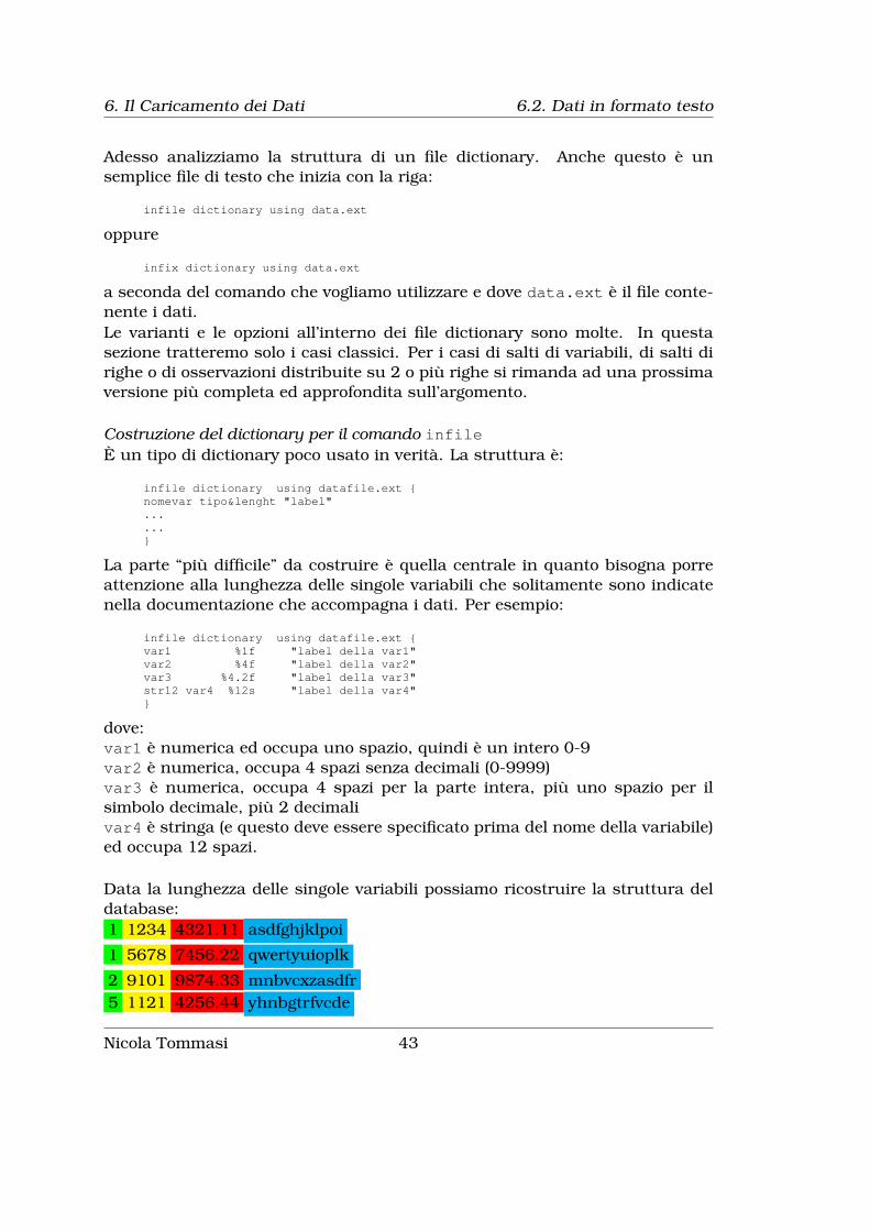
dove:var1 è numerica ed occupa uno spazio, quindi è un intero 0-9var2 è numerica, occupa 4 spazi senza decimali (0-9999)var3 è numerica, occupa 4 spazi per la parte intera, più uno spazio per ilsimbolo decimale, più 2 decimalivar4 è stringa (e questo deve essere specificato prima del nome della variabile)ed occupa 12 spazi.
Data la lunghezza delle singole variabili possiamo ricostruire la struttura deldatabase:1 1234 4321.11 asdfghjklpoi
1 5678 7456.22 qwertyuioplk
2 9101 9874.33 mnbvcxzasdfr5 1121 4256.44 yhnbgtrfvcde
Nicola Tommasi 43
6.2. Dati in formato testo 6. Il Caricamento dei Dati
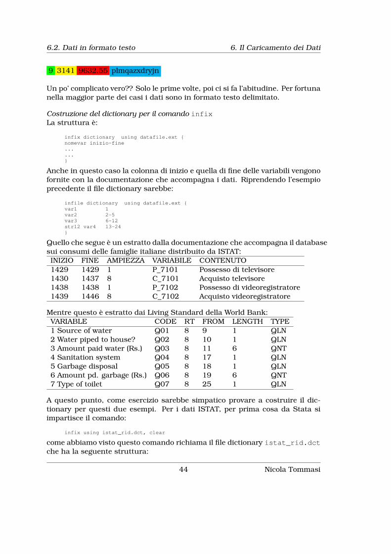
9 3141 9632.55 plmqazxdryjn
Un po’ complicato vero?? Solo le prime volte, poi ci si fa l’abitudine. Per fortunanella maggior parte dei casi i dati sono in formato testo delimitato.
Costruzione del dictionary per il comando infixLa struttura è:
infix dictionary using datafile.ext {nomevar inizio-fine......}
Anche in questo caso la colonna di inizio e quella di fine delle variabili vengonofornite con la documentazione che accompagna i dati. Riprendendo l’esempioprecedente il file dictionary sarebbe:
infile dictionary using datafile.ext {var1 1var2 2-5var3 6-12str12 var4 13-24}
Quello che segue è un estratto dalla documentazione che accompagna il databasesui consumi delle famiglie italiane distribuito da ISTAT:INIZIO FINE AMPIEZZA VARIABILE CONTENUTO1429 1429 1 P_7101 Possesso di televisore1430 1437 8 C_7101 Acquisto televisore1438 1438 1 P_7102 Possesso di videoregistratore1439 1446 8 C_7102 Acquisto videoregistratore
Mentre questo è estratto dai Living Standard della World Bank:VARIABLE CODE RT FROM LENGTH TYPE1 Source of water Q01 8 9 1 QLN2 Water piped to house? Q02 8 10 1 QLN3 Amount paid water (Rs.) Q03 8 11 6 QNT4 Sanitation system Q04 8 17 1 QLN5 Garbage disposal Q05 8 18 1 QLN6 Amount pd. garbage (Rs.) Q06 8 19 6 QNT7 Type of toilet Q07 8 25 1 QLN
A questo punto, come esercizio sarebbe simpatico provare a costruire il dic-tionary per questi due esempi. Per i dati ISTAT, per prima cosa da Stata siimpartisce il comando:
infix using istat_rid.dct, clear
come abbiamo visto questo comando richiama il file dictionary istat_rid.dctche ha la seguente struttura:
44 Nicola Tommasi

6. Il Caricamento dei Dati 6.3. Altri tipi di formati
infix dictionary using istat_rid.dat {p_7101 1429-1429c_7101 1430-1437p_7102 1438-1438c_7102 1439-1446}
il quale chiama a sua volta il file dei dati istat_rid.dat ottenendo questooutput:
. infix using istat_rid.dct, clear;
infix dictionary using istat_rid.dat {p_7101 1429-1429c_7101 1430-1437p_7102 1438-1438c_7102 1439-1446}(88 observations read)
Per il file della World Bank invece il dictionary ha la seguente struttura:
dictionary using RT008.DAT {_column( 9) byte S02C1_01 %1f "1 Source of water"_column( 10) byte S02C1_02 %1f "2 Water piped to house?"_column( 11) long S02C1_03 %6f "3 Amount paid water (Rs.)"_column( 17) byte S02C1_04 %1f "4 Sanitation system"_column( 18) byte S02C1_05 %1f "5 Garbage disposal"_column( 19) long S02C1_06 %6f "6 Amount pd. garbage (Rs.)"_column( 25) byte S02C1_07 %1f "7 Type of toilet"
}
in questo caso usiamo il comando infile ottenendo:
. infile using Z02C1, clear
dictionary using RT008.DAT {_column( 9) byte S02C1_01 %1f "1 Source of water"_column( 10) byte S02C1_02 %1f "2 Water piped to house?"_column( 11) long S02C1_03 %6f "3 Amount paid water (Rs.)"_column( 17) byte S02C1_04 %1f "4 Sanitation system"_column( 18) byte S02C1_05 %1f "5 Garbage disposal"_column( 19) long S02C1_06 %6f "6 Amount pd. garbage (Rs.)"_column( 25) byte S02C1_07 %1f "7 Type of toilet"
}
(3373 observations read)
6.3 Altri tipi di formati
Per la lettura di dati salvati in altri tipi di formati proprietari (SPSS, SAS, excel,access, . . . ) si ricorre, almeno per Stata, al programma StatTransfer3, pac-chetto commerciale che di solito si acquista in abbinamento con Stata. Questoprogramma può essere usato in maniera indipendente o chiamato direttamenteda Stata attraverso i comandi:
inputst[filetype
]infilename.ext
[switches
]3Sito web: www.stattransfer.com
Nicola Tommasi 45

6.4. Esportazione dei dati 6. Il Caricamento dei Dati
per importare dati, e
outputst[filetype
]infilename.ext
[switches
]per esportare dati. Per esempio:
inputst database.xls /yinputst database.xls /tdati /y
Nel primo caso si importano i dati del file excel database.xls, lo switch /yserve a pulire eventuali dati già in memoria; nel secondo caso si leggono i datidal file database.xls contenuti nel foglio dati. Alla stessa maniera:
outputst database.sav /y
esporta gli stessi dati in formato SPSS.
Per i dati contenuti in un file excel potete anche copiarli e incollarli diretta-mente nel 'Data editor' (e viceversa).
6.4 Esportazione dei dati
Poco fa abbiamo visto un esempio di esportazione dei dati. Se i dati devonoessere usati da altri utenti che non usano Stata è consigliabile l’esportazionein formato testo delimitato. Il comando che consiglio di usare è:
outsheet[varlist
]using
[filename
] [if
][in
][, options
]dove in filename va specificato il nome del file di output e dove le opzioniprincipali sono:
comma per avere i dati separati da ',' al posto della tabulazione che è l’opzionedi default
delimiter(char) per scegliere un delimitatore alternativo a ',' e alla tabu-lazione; per esempio ';', tipico dei files .csv
nolabel per esportare il valore numerico e non il label eventualmente asseg-nato alle variabili categoriche
replace per sovrascrivere il file di output già eventualmente creato
Una valida alternativa al formato testo puro è il formato XML. Si definisce comeun file di testo strutturato ed ha il vantaggio della portabilità tra le applicazioniche lo supportano. Esistono 2 versioni del comando. Questa salva il datasetin memoria nel formato XML:
xmlsave filename[if
][in
][, xmlsave_options
]Questa salva il sottoinsieme delle variabili specificate:
xmlsave[varlist
]using filename
[if
][in
][, xmlsave_options
]le possibili xmlsave_options sono:
46 Nicola Tommasi

6. Il Caricamento dei Dati 6.5. Cambiare temporaneamente dataset
doctype(dta) salva il file XML usando le specifiche determinate da Stata peri files .dta
doctype(excel) salva il file XML usando le specifiche determinate per i filesExcel
dtd include il DTD (Document Type Definition) nel file XML. Questa opzione èusata raramente ed inoltre aumenta la dimensione finale del file
legible fa in modo che il file XML visivamente più leggibile. Attenzione cheanche questa opzione aumenta la dimensione finale del file
replace sovrascrive un eventuale filename già esistente
Per inciso, per leggere i dati salvati in XML si usa il comando
xmluse filename[, xmluse_options
]che qui non viene trattatoTutti sappiamo che excel è il formato più diffuso per salvare dati (purtroppo!),ma per favore evitate di esportare i dati in tale formato, poiché excel ha il bruttovizio (ma non è il solo) di “interpretare” i dati come in questo caso:
01.11.5 P / 01.24 S01.11.5 P / 01.24 S01.11.5 P / 01.21 S01.11.5 P / 01.2 S1:11:05 PM1:11:05 PM1:11:05 PM
Gli ultimi tre casi sono stati interpretati da excel come delle ore, invece sonocodici ateco (per la precisione codice 01.11.05).
6.5 Cambiare temporaneamente dataset
Come abbiamo già detto Stata consente l’utilizzo di un solo dataset alla volta.Può allora risultare scomodo salvare il dataset sul quale si sta’ lavorando perdedicarsi temporaneamente ad un altro e poi riprendere il primo. In questi casipossiamo ricorrere all’accoppiata di comandi
preserve
restore
Con preserve iberniamo il dataset sul quale stiamo lavorando; possiamo quin-di fare dei cambiamenti su questo dataset o passare ad utilizzarne un altro.In seguito con il comando restore ritorniamo ad utilizzare il dataset prece-dentemente ibernato. Nell’esempio che segue si parte con un dataset e dopo ilcomando preserve si prendono solo alcune variabili, si salva il dataset e poisi torna a quello di partenza:
. desc, short;
Nicola Tommasi 47
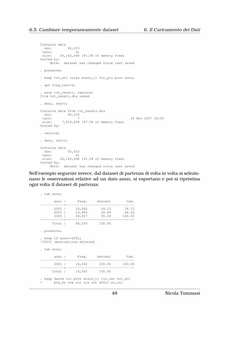
6.5. Cambiare temporaneamente dataset 6. Il Caricamento dei Dati
Contains dataobs: 92,033vars: 41size: 28,162,098 (91.0% of memory free)Sorted by:
Note: dataset has changed since last saved
. preserve;
. keep tot_att cciaa ateco_1l for_giu prov anno;
. gen flag_test=0;
. save tot_veneto, replace;file tot_veneto.dta saved
. desc, short;
Contains data from tot_veneto.dtaobs: 92,033vars: 7 26 Nov 2007 18:00size: 7,914,838 (97.5% of memory free)Sorted by:
. restore;
. desc, short;
Contains dataobs: 92,033vars: 41size: 28,162,098 (91.0% of memory free)Sorted by:
Note: dataset has changed since last saved
Nell’esempio seguente invece, dal dataset di partenza di volta in volta si selezio-nano le osservazioni relative ad un dato anno, si esportano e poi si ripristinaogni volta il dataset di partenza:
. tab anno;
anno | Freq. Percent Cum.------------+-----------------------------------
2001 | 16,062 18.13 18.132003 | 23,464 26.49 44.622005 | 49,067 55.38 100.00
------------+-----------------------------------Total | 88,593 100.00
. preserve;
. keep if anno==2001;(72531 observations deleted)
. tab anno;
anno | Freq. Percent Cum.------------+-----------------------------------
2001 | 16,062 100.00 100.00------------+-----------------------------------
Total | 16,062 100.00
. keep denom loc prov ateco_1l ric_ven tot_att> pos_fn roe roi ros rot effic ac_ric
48 Nicola Tommasi
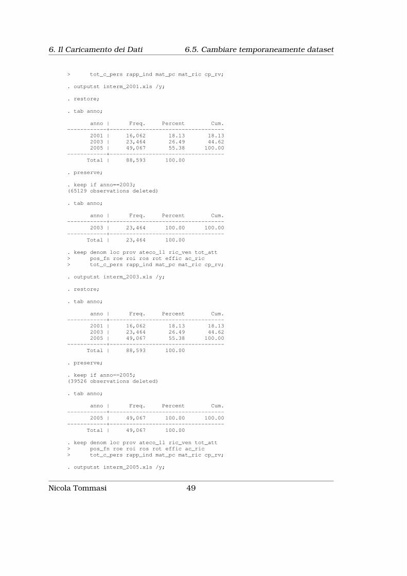
6. Il Caricamento dei Dati 6.5. Cambiare temporaneamente dataset
> tot_c_pers rapp_ind mat_pc mat_ric cp_rv;
. outputst interm_2001.xls /y;
. restore;
. tab anno;
anno | Freq. Percent Cum.------------+-----------------------------------
2001 | 16,062 18.13 18.132003 | 23,464 26.49 44.622005 | 49,067 55.38 100.00
------------+-----------------------------------Total | 88,593 100.00
. preserve;
. keep if anno==2003;(65129 observations deleted)
. tab anno;
anno | Freq. Percent Cum.------------+-----------------------------------
2003 | 23,464 100.00 100.00------------+-----------------------------------
Total | 23,464 100.00
. keep denom loc prov ateco_1l ric_ven tot_att> pos_fn roe roi ros rot effic ac_ric> tot_c_pers rapp_ind mat_pc mat_ric cp_rv;
. outputst interm_2003.xls /y;
. restore;
. tab anno;
anno | Freq. Percent Cum.------------+-----------------------------------
2001 | 16,062 18.13 18.132003 | 23,464 26.49 44.622005 | 49,067 55.38 100.00
------------+-----------------------------------Total | 88,593 100.00
. preserve;
. keep if anno==2005;(39526 observations deleted)
. tab anno;
anno | Freq. Percent Cum.------------+-----------------------------------
2005 | 49,067 100.00 100.00------------+-----------------------------------
Total | 49,067 100.00
. keep denom loc prov ateco_1l ric_ven tot_att> pos_fn roe roi ros rot effic ac_ric> tot_c_pers rapp_ind mat_pc mat_ric cp_rv;
. outputst interm_2005.xls /y;
Nicola Tommasi 49

6.5. Cambiare temporaneamente dataset 6. Il Caricamento dei Dati
. restore;
. tab anno;
anno | Freq. Percent Cum.------------+-----------------------------------
2001 | 16,062 18.13 18.132003 | 23,464 26.49 44.622005 | 49,067 55.38 100.00
------------+-----------------------------------Total | 88,593 100.00
50 Nicola Tommasi

Capitolo 7
Gestione delle Variabili
7.1 Descrizione di variabili e di valori
Bene, adesso abbiamo caricato il database in Stata ma per renderlo intellegibileoccorre:
a. Descrivere il dataset (questo non è così indispensabile!)b. Descrivere le variabili (questo invece sì)c. Descrivere i valori delle variabili categoriche (e anche questo)
Per prima cosa diamo una prima occhiata al dataset sfruttando l’output di duecomandi:
describe[varlist
][, memory_options
]che descrive il dataset senza troncare i nomi troppo lunghi delle variabili.
. desc, full
Contains data from C:/Programmi/Stata9/ado/base/u/uslifeexp.dtaobs: 100 U.S. life expectancy, 1900-1999vars: 10 30 Mar 2005 04:31size: 4,200 (99.9% of memory free) (_dta has notes)------------------------------------------------------------------------------
storage display valuevariable name type format label variable label------------------------------------------------------------------------------year int %9.0g Yearle float %9.0g life expectancyle_male float %9.0g Life expectancy, malesle_female float %9.0g Life expectancy, femalesle_w float %9.0g Life expectancy, whitesle_wmale float %9.0g Life expectancy, white malesle_wfemale float %9.0g Life expectancy, white femalesle_b float %9.0g Life expectancy, blacksle_bmale float %9.0g Life expectancy, black malesle_bfemale float %9.0g Life expectancy, black females------------------------------------------------------------------------------Sorted by: year
Opzioni interessanti del comando sono:
51
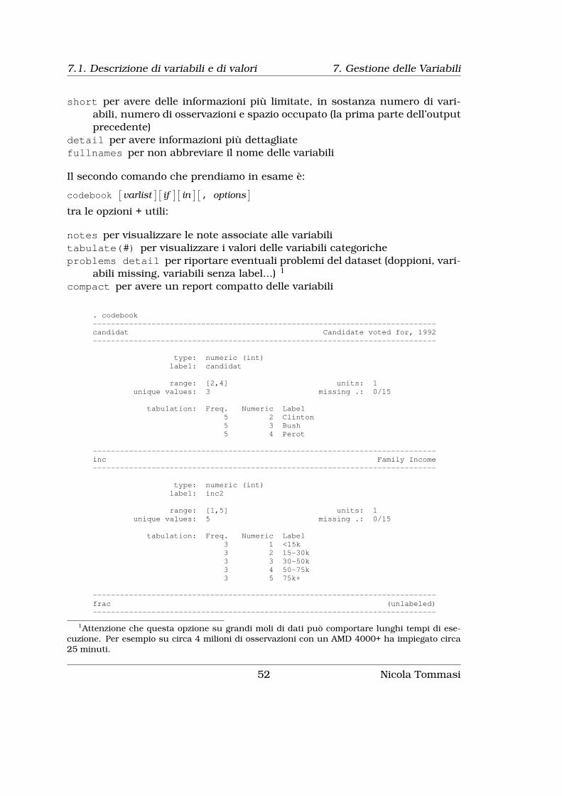
7.1. Descrizione di variabili e di valori 7. Gestione delle Variabili
short per avere delle informazioni più limitate, in sostanza numero di vari-abili, numero di osservazioni e spazio occupato (la prima parte dell’outputprecedente)
detail per avere informazioni più dettagliatefullnames per non abbreviare il nome delle variabili
Il secondo comando che prendiamo in esame è:
codebook[varlist
][if
][in
][, options
]tra le opzioni + utili:
notes per visualizzare le note associate alle variabilitabulate(#) per visualizzare i valori delle variabili categoricheproblems detail per riportare eventuali problemi del dataset (doppioni, vari-
abili missing, variabili senza label...) 1
compact per avere un report compatto delle variabili
. codebook----------------------------------------------------------------------------candidat Candidate voted for, 1992----------------------------------------------------------------------------
type: numeric (int)label: candidat
range: [2,4] units: 1unique values: 3 missing .: 0/15
tabulation: Freq. Numeric Label5 2 Clinton5 3 Bush5 4 Perot
----------------------------------------------------------------------------inc Family Income----------------------------------------------------------------------------
type: numeric (int)label: inc2
range: [1,5] units: 1unique values: 5 missing .: 0/15
tabulation: Freq. Numeric Label3 1 <15k3 2 15-30k3 3 30-50k3 4 50-75k3 5 75k+
----------------------------------------------------------------------------frac (unlabeled)----------------------------------------------------------------------------
1Attenzione che questa opzione su grandi moli di dati può comportare lunghi tempi di ese-cuzione. Per esempio su circa 4 milioni di osservazioni con un AMD 4000+ ha impiegato circa25 minuti.
52 Nicola Tommasi
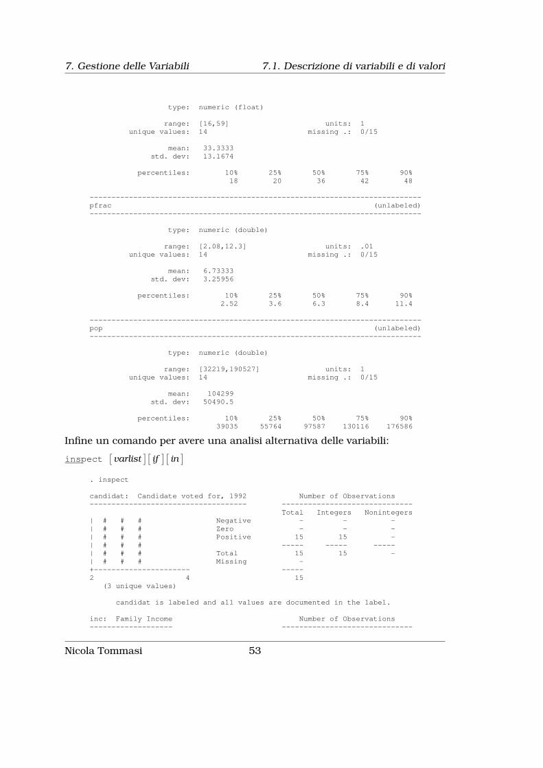
7. Gestione delle Variabili 7.1. Descrizione di variabili e di valori
type: numeric (float)
range: [16,59] units: 1unique values: 14 missing .: 0/15
mean: 33.3333std. dev: 13.1674
percentiles: 10% 25% 50% 75% 90%18 20 36 42 48
----------------------------------------------------------------------------pfrac (unlabeled)----------------------------------------------------------------------------
type: numeric (double)
range: [2.08,12.3] units: .01unique values: 14 missing .: 0/15
mean: 6.73333std. dev: 3.25956
percentiles: 10% 25% 50% 75% 90%2.52 3.6 6.3 8.4 11.4
----------------------------------------------------------------------------pop (unlabeled)----------------------------------------------------------------------------
type: numeric (double)
range: [32219,190527] units: 1unique values: 14 missing .: 0/15
mean: 104299std. dev: 50490.5
percentiles: 10% 25% 50% 75% 90%39035 55764 97587 130116 176586
Infine un comando per avere una analisi alternativa delle variabili:
inspect[varlist
][if
][in
]. inspect
candidat: Candidate voted for, 1992 Number of Observations------------------------------------ ------------------------------
Total Integers Nonintegers| # # # Negative - - -| # # # Zero - - -| # # # Positive 15 15 -| # # # ----- ----- -----| # # # Total 15 15 -| # # # Missing -+---------------------- -----2 4 15
(3 unique values)
candidat is labeled and all values are documented in the label.
inc: Family Income Number of Observations------------------- ------------------------------
Nicola Tommasi 53
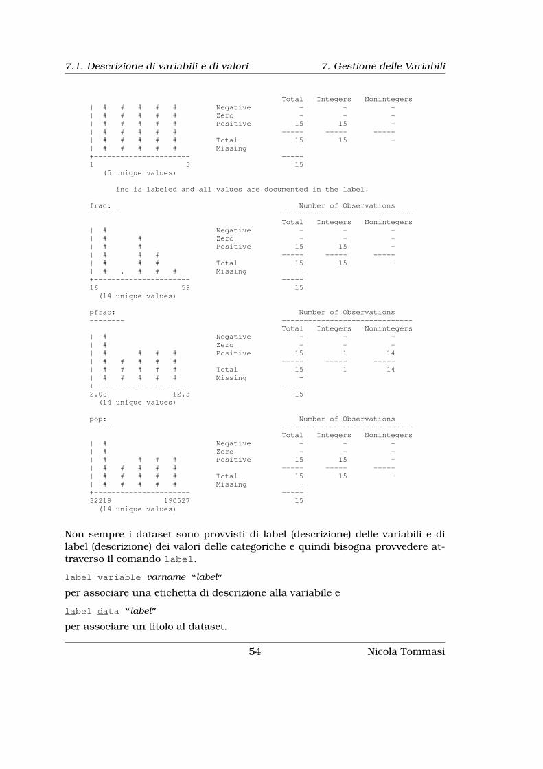
7.1. Descrizione di variabili e di valori 7. Gestione delle Variabili
Total Integers Nonintegers| # # # # # Negative - - -| # # # # # Zero - - -| # # # # # Positive 15 15 -| # # # # # ----- ----- -----| # # # # # Total 15 15 -| # # # # # Missing -+---------------------- -----1 5 15
(5 unique values)
inc is labeled and all values are documented in the label.
frac: Number of Observations------- ------------------------------
Total Integers Nonintegers| # Negative - - -| # # Zero - - -| # # Positive 15 15 -| # # # ----- ----- -----| # # # Total 15 15 -| # . # # # Missing -+---------------------- -----16 59 15
(14 unique values)
pfrac: Number of Observations-------- ------------------------------
Total Integers Nonintegers| # Negative - - -| # Zero - - -| # # # # Positive 15 1 14| # # # # # ----- ----- -----| # # # # # Total 15 1 14| # # # # # Missing -+---------------------- -----2.08 12.3 15
(14 unique values)
pop: Number of Observations------ ------------------------------
Total Integers Nonintegers| # Negative - - -| # Zero - - -| # # # # Positive 15 15 -| # # # # # ----- ----- -----| # # # # # Total 15 15 -| # # # # # Missing -+---------------------- -----32219 190527 15
(14 unique values)
Non sempre i dataset sono provvisti di label (descrizione) delle variabili e dilabel (descrizione) dei valori delle categoriche e quindi bisogna provvedere at-traverso il comando label.
label variable varname “label”
per associare una etichetta di descrizione alla variabile e
label data “label”
per associare un titolo al dataset.
54 Nicola Tommasi
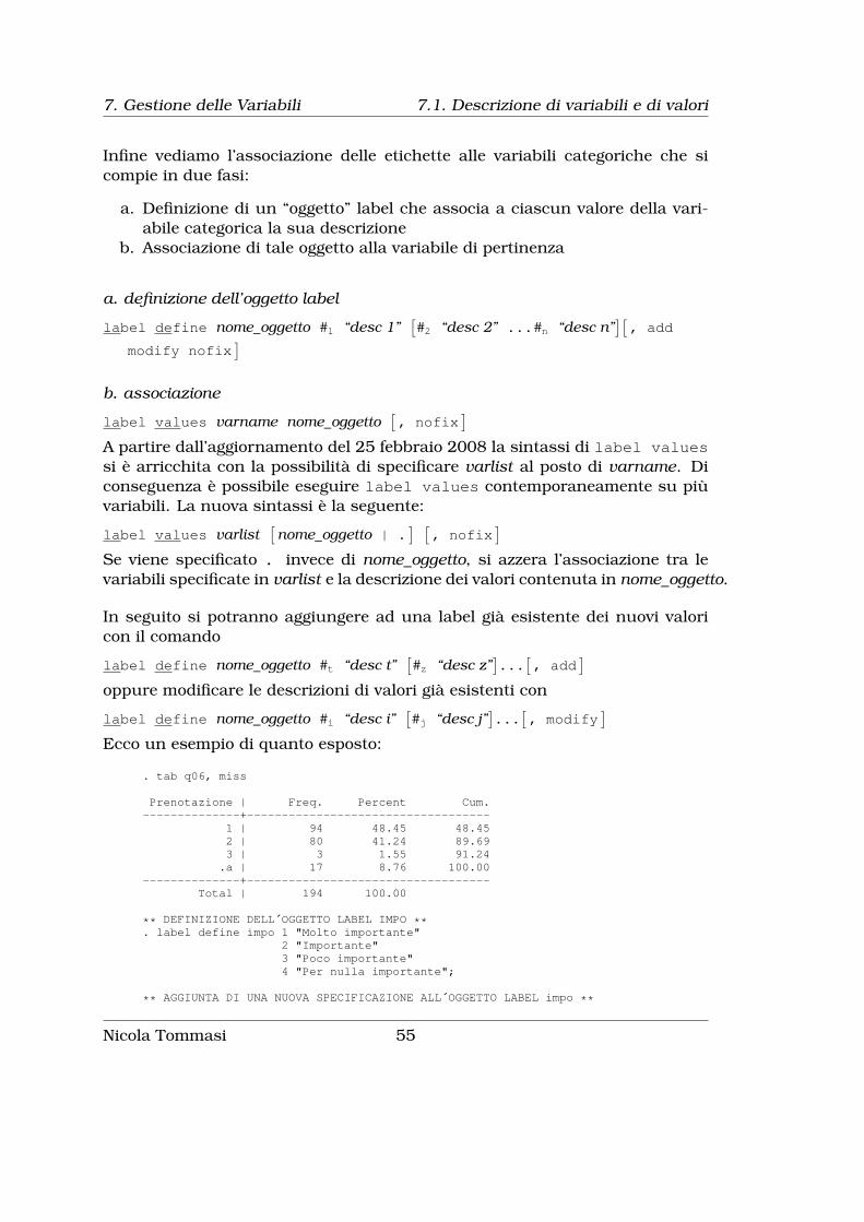
7. Gestione delle Variabili 7.1. Descrizione di variabili e di valori
Infine vediamo l’associazione delle etichette alle variabili categoriche che sicompie in due fasi:
a. Definizione di un “oggetto” label che associa a ciascun valore della vari-abile categorica la sua descrizione
b. Associazione di tale oggetto alla variabile di pertinenza
a. definizione dell’oggetto label
label define nome_oggetto #1 “desc 1”[#2 “desc 2” ...#n “desc n”
][, add
modify nofix]
b. associazione
label values varname nome_oggetto[, nofix
]A partire dall’aggiornamento del 25 febbraio 2008 la sintassi di label valuessi è arricchita con la possibilità di specificare varlist al posto di varname. Diconseguenza è possibile eseguire label values contemporaneamente su piùvariabili. La nuova sintassi è la seguente:
label values varlist[nome_oggetto | .
] [, nofix
]Se viene specificato . invece di nome_oggetto, si azzera l’associazione tra levariabili specificate in varlist e la descrizione dei valori contenuta in nome_oggetto.
In seguito si potranno aggiungere ad una label già esistente dei nuovi valoricon il comando
label define nome_oggetto #t “desc t”[#z “desc z”
]...
[, add
]oppure modificare le descrizioni di valori già esistenti con
label define nome_oggetto #i “desc i”[#j “desc j”
]...
[, modify
]Ecco un esempio di quanto esposto:
. tab q06, miss
Prenotazione | Freq. Percent Cum.--------------+-----------------------------------
1 | 94 48.45 48.452 | 80 41.24 89.693 | 3 1.55 91.24.a | 17 8.76 100.00
--------------+-----------------------------------Total | 194 100.00
** DEFINIZIONE DELL´OGGETTO LABEL IMPO **. label define impo 1 "Molto importante"
2 "Importante"3 "Poco importante"4 "Per nulla importante";
** AGGIUNTA DI UNA NUOVA SPECIFICAZIONE ALL´OGGETTO LABEL impo **
Nicola Tommasi 55

7.1. Descrizione di variabili e di valori 7. Gestione delle Variabili
. label define impo .a "Non risponde", add;
*ASSOCIAZIONE ALLA VARIABILE q06 DELL´OGGETTO LABEL impo **. label values q06 impo;. tab q06, miss
Prenotazione | Freq. Percent Cum.---------------------+-----------------------------------
Molto importante | 94 48.45 48.45Importante | 80 41.24 89.69
Poco importante | 3 1.55 91.24Non risponde | 17 8.76 100.00
---------------------+-----------------------------------Total | 194 100.00
La panoramica sul comando label si conclude con:
label dir per avere la lista degli oggetti labellabel list nome_oggetto per vedere i valori delle labellabel drop nome_oggetto | _all per eliminare una label o per eliminarle
tutte
. label dir
impoulsscod_comepd1epd2
. label list impo
impo:1 Molto importante2 Importante3 Poco importante4 Per nulla importante.a Non risponde
Naturalmente, una volta definito un oggetto label lo si può associare a piùvariabili usando il comando label values.
label values q06 q08 q11 q17 q23 impo
Per manipolare le labels possiamo ricorrere al comando
labvalch valuelabelname,[{from(numlist) to(numlist) | swap(#1 #2) }
delete(numlist) list]
che consente operazioni di copia/trasferimento e cancellazione delle value la-bels. Una volta specificato un set di valori label possiamo convertire labelattraverso questo procedimento:
from(numlist) qui si specificano i valori numerici da trasferireto(numlist) qui si specificano i valori numerici che assumeranno le nuove
label
56 Nicola Tommasi

7. Gestione delle Variabili 7.1. Descrizione di variabili e di valori
in from() e to() ci devono essere gli stessi numeri. Se per esempio abbiamo ilset di valori denominato rating e che assume i valori 1 “poor” 2 “fair” 3 “OK” 4“good” 5 “excellent” e vogliamo invertirne l’ordine
labvalch rating, from(1/5) to(5/1)
Con swap(#1 #2) specifico 2 valori della label che voglio vengano scambiatimentre con delete(numlist) indico la lista delle label che desidero eliminare
Potrebbero tornare utili anche i comandi labelbook e numlabel. labelbookproduce un rapporto di descrizione delle label:
labelbook[lblname-list
] [, labelbook_options
]labelbook_options:
alpha ordina le label in ordine alfabetico anziché in base alla numerazioneassegnata
length(#) controlla se ci sono label uguali fino alla lunghezza specificata in#; il valore di default è length(12) dato che questa lunghezza è quellatipicamente usata nell’output dei comandi (tabulate per esempio)
problems descrive potenziali problemi delle label come per esempio:
1. buchi nei valori mappati (per esempio esistono i valori 1 e 3 ma nonil valore 2)
2. le descrizioni contengono spazi all’inizio o alla fine3. stesse descrizioni associate a valori diversi4. label identiche fino alla lunghezza di 12 caratteri5. valori di una label non usati da nessuna variabile
detail produce un rapporto dettagliato sulle variabili e sulle label
. desc d02 d03 d07 d10_1
storage display valuevariable name type format label variable label--------------------------------------------------------------------------------------------------------------------------------------------d02 byte %12.0g D02 Sessod03 byte %23.0g D03 Istruzioned07 byte %12.0g D07 Tipo di ricoverod10_1 byte %25.0g D10 Medici
. labelbook D02 D03 D07 D10, problems detail
--------------------------------------------------------------------------------------------------------------------------------------------value label D02--------------------------------------------------------------------------------------------------------------------------------------------
values labelsrange: [1,2] string length: [7,12]
N: 3 unique at full length: yesgaps: no unique at length 12: yes
missing .*: 1 null string: noleading/trailing blanks: no
numeric -> numeric: nodefinition
Nicola Tommasi 57

7.1. Descrizione di variabili e di valori 7. Gestione delle Variabili
1 Maschio2 Femmina.a Non risponde
variables: d02
--------------------------------------------------------------------------------------------------------------------------------------------value label D03--------------------------------------------------------------------------------------------------------------------------------------------
values labelsrange: [1,5] string length: [6,23]
N: 6 unique at full length: yesgaps: no unique at length 12: yes
missing .*: 1 null string: noleading/trailing blanks: no
numeric -> numeric: nodefinition
1 Nessun titolo2 Licenza elementare3 Licenza media inferiore4 Diploma media superiore5 Laurea.a Non risponde
variables: d03
--------------------------------------------------------------------------------------------------------------------------------------------value label D07--------------------------------------------------------------------------------------------------------------------------------------------
values labelsrange: [1,2] string length: [7,12]
N: 3 unique at full length: yesgaps: no unique at length 12: yes
missing .*: 1 null string: noleading/trailing blanks: no
numeric -> numeric: nodefinition
1 Urgente2 Programmato.a Non risponde
variables: d07
--------------------------------------------------------------------------------------------------------------------------------------------value label D10--------------------------------------------------------------------------------------------------------------------------------------------
values labelsrange: [1,6] string length: [10,25]
N: 7 unique at full length: yesgaps: no unique at length 12: yes
missing .*: 1 null string: noleading/trailing blanks: no
numeric -> numeric: nodefinition
1 Per nulla soddisfatto2 Poco soddisfatto3 Soddisfatto4 Più che Soddisfatto5 Completamente Soddisfatto
58 Nicola Tommasi

7. Gestione delle Variabili 7.1. Descrizione di variabili e di valori
6 Non saprei.a Non risponde
variables: d10_1 d10_2 d10_3 d10_4 d10_5 d10_6
no potential problems in dataset C:/Projects/s_cuore/sodd_paz_2008/data/mother.dta
numlabel aggiunge come prefisso numerico il valore della label
numlabel[lblname-list
] [, {add|remove} numlabel_options
]numlabel_options:
add aggiunge il prefisso numerico alle labelremove rimuove il prefisso numerico alle labelmask(str) maschera di formattazione per l’aggiunta del valore numerico; di
default la maschera è “#.”force forza l’aggiunta o la rimozione del valore numericodetail visualizza esempio di label con e senza il prefisso numerico
. numlabel D10, add
. tab d10_1, miss
Medici | Freq. Percent Cum.-----------------------------+-----------------------------------
1. Per nulla soddisfatto | 2 0.14 0.142. Poco soddisfatto | 4 0.29 0.43
3. Soddisfatto | 208 14.97 15.414. Più che Soddisfatto | 356 25.63 41.04
5. Completamente Soddisfatto | 747 53.78 94.826. Non saprei | 5 0.36 95.18
.a. Non risponde | 67 4.82 100.00-----------------------------+-----------------------------------
Total | 1,389 100.00
. numlabel D10, remove
. numlabel D10, add mask([#.] )
. tab d10_1, miss
Medici | Freq. Percent Cum.------------------------------+-----------------------------------
[1.]Per nulla soddisfatto | 2 0.14 0.14[2.]Poco soddisfatto | 4 0.29 0.43
[3.]Soddisfatto | 208 14.97 15.41[4.]Più che Soddisfatto | 356 25.63 41.04
[5.]Completamente Soddisfatto | 747 53.78 94.82[6.]Non saprei | 5 0.36 95.18
[.a.]Non risponde | 67 4.82 100.00------------------------------+-----------------------------------
Total | 1,389 100.00
Utili comandi aggiuntivi sono le labutil (ssc inst labutil) che consentonotra l’altro di utilizzare una variabile per creare il label define per un’altra(labmask).
Nicola Tommasi 59

7.1. Descrizione di variabili e di valori 7. Gestione delle Variabili
È anche possibile inserire delle note al dataset o a singole variabili con
notes[varname
]: text
se non viene specificata nessuna varname la nota viene riferita all’intero dataset,altrimenti alla variabile specificata. Poi visualizzarle si usa il comando
notes[list
]note: Valori espressi in Euronote y1: escluso da capitale finanziario.note y1: y1 = (yl + yt + ym + yca)note y2: y2 = (yl + yt + ym + yc)note yl: yl = (yl1 + yl2)note yt: yt = (ytp + yta)note ytp: ytp = (ytp1 + ytp2)
notes
_dta:1. Valori espressi in Euro
y1:1. escluso da capitale finanziario.2. y1 = (yl + yt + ym + yca)
y2:1. y2 = (yl + yt + ym + yc)
yl:1. yl = (yl1 + yl2)
yt:1. yt = (ytp + yta)
ytp:1. ytp = (ytp1 + ytp2)
codebook y1, all
-----------------------------------------------------------------------------y1 Reddito disponibile netto-----------------------------------------------------------------------------
type: numeric (float)
range: [0,418846.53] units: .01unique values: 2910 missing .: 6/7147
mean: 24801std. dev: 18549
percentiles: 10% 25% 50% 75% 90%8263.31 13427.9 21174.7 31865.4 43950.5
y1:1. escluso da capitale finanziario.2. y1 = (yl + yt + ym + yca)
60 Nicola Tommasi

7. Gestione delle Variabili 7.2. Controllo delle variabili chiave
7.2 Controllo delle variabili chiave
Cosa sono le variabili chiave? È quella variabile o quell’insieme di variabiliche permettono di identificare in maniera univoca ciascuna osservazione deldataset. Sapere quali sono le variabili chiave è fondamentale per applicarecorrettamente una serie di comandi (merge per esempio) e per interpretare irisultati delle analisi. Stata dispone di un set di istruzioni dedicate alla gestionedelle variabili chiave. Il principale è:
duplicates report[varlist
][if
][in
]che controlla se le variabili specificate in varlist sono delle variabili chiave.
. duplicates report idcode
Duplicates in terms of idcode--------------------------------------
copies | observations surplus----------+---------------------------
1 | 2246 0--------------------------------------
in questo caso la variabile idcode è variabili chiave perché non ci sono doppi-oni, mentre nel caso seguente
. duplicates report fam_id
Duplicates in terms of fam_id--------------------------------------
copies | observations surplus----------+---------------------------
1 | 6303 02 | 14646 73233 | 18846 125644 | 23956 179675 | 8330 66646 | 2022 16857 | 595 5108 | 112 989 | 27 2410 | 20 1811 | 11 1012 | 12 11
--------------------------------------
fam_id non è variabile chiave perché ci sono osservazioni doppie (14646), triple(18846) e così via.Se siamo sicuri che ci siano effettivamente delle osservazioni ripetute (il chevuol dire che tutte le variabili dell’osservazione hanno valori uguali e non soloper le variabili chiave), possiamo ricorrere a questo comando per eliminarle:
duplicates drop varlist[if
][in
], force
quindi ritornando all’esempio precedente:
duplicates drop fam_id, force
Duplicates in terms of fam_id(46874 observations deleted)
Nicola Tommasi 61

7.3. Rinominare variabili 7. Gestione delle Variabili
7.3 Rinominare variabili
Il comando di Stata per cambiare il nome ad una variabile è:
rename old_varname new_varname
ma molto più potente e ricco di funzioni è il comando aggiuntivo renvars2
nella versione:
renvars[varlist
]\ newvarlist
[, display test
]che rinomina le variabili della lista prima del simbolo \ con le corrispondentiche lo seguono. Le opzioni
display serve per vedere ciascun cambiamentotest serve per testare la modifica senza eseguirla
Ma ancora più interessante è la versione:
renvars[varlist
], transformation_option
[, display test symbol(string)
]con transformation_option che possono essere una tra:
upper per convertire i nomi in maiuscololower per convertire i nomi in minuscoloprefix(str) per assegnare il prefisso str al nome delle variabilipostfix(str) per assegnare str come finale del nome delle variabilisubst(str1 str2) per sostituire tutte le ricorrenze str1 con str2 (str2 può anche
essere vuoto)trim(#) per prendere solo i primi # caratteri del nometrimend(#) per prendere solo gli ultimi # caratteri del nome
Ecco alcuni esempi con le opzioni appena viste:Esempi di rename classico:
rename c2 TM1rename c3 TM2rename c4 TM3rename c5 TM4rename c6 TM5rename c7 TM6rename c8 TM7rename c9 TM8rename c10 TM9
Esempi di renvars:
. renvars c2-c10 TM1-TM9 , display test;specification would result in the following renames:
c2 -> TM1c3 -> TM2c4 -> TM3
2Come si fa ad installarlo? Dovreste essere in grado di farlo!
62 Nicola Tommasi

7. Gestione delle Variabili 7.4. Ordinare variabili
c5 -> TM4c6 -> TM5c7 -> TM6c8 -> TM7c9 -> TM8c10 -> TM9
. renvars c2-c10, upper test;specification would result in the following renames:
c2 -> C2c3 -> C3c4 -> C4c5 -> C5c6 -> C6c7 -> C7c8 -> C8c9 -> C9c10 -> C10
. renvars c2-c10, prefix(tax_) test;specification would result in the following renames:
c2 -> tax_c2c3 -> tax_c3c4 -> tax_c4c5 -> tax_c5c6 -> tax_c6c7 -> tax_c7c8 -> tax_c8c9 -> tax_c9c10 -> tax_c10
. renvars c2-c10, postfix(t) test;specification would result in the following renames:
c2 -> c2tc3 -> c3tc4 -> c4tc5 -> c5tc6 -> c6tc7 -> c7tc8 -> c8tc9 -> c9tc10 -> c10t
7.4 Ordinare variabili
Per ordinare le osservazioni in base ai valori di una o più variabili si usa ilcomando
sort varlist[in
][, stable
]Alternativamente si può usare il più sofisticato
gsort[+|-
]varname
[ [+|-
]varname ...
] [, generate(newvar) mfirst
]il segno + (ordinamento crescente) si può omettere per ordinare in senso cres-cente. Da notare che si può anche combinare un ordinamento in senso cres-cente per una variabile con l’ordinamento in senso decrescente (-) di un’altra3.Questo comando funziona anche con variabili stringa.
3Come vengono ordinati i valori missing?
Nicola Tommasi 63

7.5. Prendere o scartare osservazioni o variabili 7. Gestione delle Variabili
ESEMPIO opzione stable
Invece per spostare le variabili all’inizio della lista si usa:
order varlist
. desc, simplebalance id var1
. order id
. desc, simpleid balance var1
Per spostare varname1 al posto di varname2:
move varname1 varname2
. desc, simpleid balance var1
. move var1 balance
. desc, simpleid var1 balance
Per ordinare in senso alfabetico in base al nome della variabile:
aorder[varlist
]. desc, simpleid var1 balance
. aorder
. desc, simplebalance id var1
7.5 Prendere o scartare osservazioni o variabili
La coppia di comandi keep e drop serve per tenere (keep) variabili o osser-vazioni, oppure a cancellare (drop) variabili o osservazioni.Per tenere variabili, scartando le altre:
keep varlist
Per tenere osservazioni, scartando le altre:
keep if condizione
Per eliminare variabili, tenendo le altre:
drop varlist
Per eliminare osservazioni, tenendo le altre
drop if condizione
64 Nicola Tommasi

7. Gestione delle Variabili 7.5. Prendere o scartare osservazioni o variabili
Esiste anche un comando per estrarre da un database un campione casualedi una determinata numerosità. Prima di analizzarlo però vediamo come siapossibile creare “un campione casuale sempre uguale”. In genere per produrreun campione casuale si genera un numero casuale detto seme e sulla base diquesto si genera l’algoritmo per l’estrazione del campione. Fissando il valoredi questo seme, il campione casuale estratto sarà, di conseguenza, sempreuguale. Il comando:
set seed #
serve proprio a questo.
Il comando per estrarre il campione casuale è invece:
sample #[if
][in
][, count by(groupvars)
]dove # è la percentuale delle osservazioni del dataset di partenza che deve avereil campione casuale. Se invece vogliamo avere l’estrazione di un determinatonumero di osservazioni, occorre usare l’opzione count e # sarà il numero diosservazioni da estrarre. Ecco gli esempi per i due casi:
. use ita_82-06, clear
. desc, short
Contains data from ita_82-06.dtaobs: 1,636,402vars: 33 4 Jul 2007 13:19size: 121,093,748 (53.8% of memory free)Sorted by:
Note: dataset has changed since last saved
. set seed 74638928
. summ pop_2006
Variable | Obs Mean Std. Dev. Min Max-------------+--------------------------------------------------------
pop_2006 | 1636402 35.90298 219.7405 0 23722
. sample 20(1309122 observations deleted)
. summ pop_2006
Variable | Obs Mean Std. Dev. Min Max-------------+--------------------------------------------------------
pop_2006 | 327280 35.03108 203.4676 0 23329
. sample 2380, count(324900 observations deleted)
. summ pop_2006
Variable | Obs Mean Std. Dev. Min Max-------------+--------------------------------------------------------
pop_2006 | 2380 38.21765 181.8105 0 6615
Nicola Tommasi 65
7.6. Gestire il formato delle variabili 7. Gestione delle Variabili
7.6 Gestire il formato delle variabili
Stata salva le variabili in diversi formati numerici a seconda delle necessità.L’obiettivo è di minimizzare lo spazio di memoria occupato da ciascuna vari-abile. Per esempio è inutile sprecare spazio per i decimali per una variabileche può assumere solo valori interi o dedicare 100 caratteri per una variabilestringa quando al massimo arriva a 70. Segue lo schema delle classi di variabilisupportate in Stata:Stringastr# con massimo 244 caratteri di lunghezza
Numeriche
byte numeri interi tra -127 e 100;int numeri interi tra -32 740 e 32 740;long numeri interi tra -2 147 483 647 e 2 147 483 620;float numeri reali con 8 cifre decimali di accuratezza compresi tra -1.70141173319*10ˆ38
e 1.70141173319*10ˆ36;double numeri reali con 17 cifre decimali di accuratezza compresi tra -8.9884656743*10ˆ307
e 8.9884656743*10ˆ307.
Passando da byte a int, a long e a float la quantità di memoria occupata dauna variabile aumenta. Il modo più semplice per ottimizzare lo spazio occupatoda ciascuna variabile è il comando compress, che abbiamo già visto, altrimentise vogliamo forzare una certa variabile ad avere un certo formato possiamousare:
recast type varlist[, force
]dove type può assumere i valori -byte
-int-long-float-double-str#
Discorso diverso è il formato con cui una variabile viene visualizzata e cheè indipendente dal formato con cui viene salvata/trattata. In questo casodobbiamo far ricorso al comando:
format %fmt varlist
dove %fmt può assumere le seguenti forme:
66 Nicola Tommasi

7. Gestione delle Variabili 7.6. Gestire il formato delle variabili
Numerical%fmt Description Example
-------------------------------------------------------right justified
%#.#g general %9.0g%#.#f fixed %9.2f%#.#e exponential %10.7e%21x hexadecimal %21x%16H binary, hilo %16H%16L binary, lohi %16L%8H binary, hilo %8H%8L binary, lohi %8L
right justified with commas%#.#gc general %9.0gc%#.#fc fixed %9.2fc
right justified with leading zeros%0#.#f fixed %09.2f
left justified%-#.#g general %-9.0g%-#.#f fixed %-9.2f%-#.#e exponential %-10.7e
left justified with commas%-#.#gc general %-9.0gc%-#.#fc fixed %-9.2fc
-------------------------------------------------------You may substitute comma (,) for period (.) in any ofthe above formats to make comma the decimal point. In%9,2fc, 1000.03 is 1.000,03. Or you can set dp comma.
date%fmt Description Example
-------------------------------------------------------right justified
%tc date/time %tc%tC date/time %tC%td date %td%tw week %tw%tm month %tm
Nicola Tommasi 67

7.6. Gestire il formato delle variabili 7. Gestione delle Variabili
%tq quarter %tq%th halfyear %th%ty year %ty%tg generic %tg
left justified%-tc date/time %-tc%-tC date/time %-tC%-td date %-tdetc.
-------------------------------------------------------There are lots of variations allowed. See Formattingdate and time values in [D] dates and times.
string%fmt Description Example
-------------------------------------------------------right justified
%#s string %15s
left justified%-#s string %-20s
centered%~#s string %~12s
-------------------------------------------------------The centered format is for use with display only.
Aggiungo che si può modificare come Stata rappresenta il simbolo decimalecon il comando
set dp {comma|period}[, permanently
]. di 123.79123.79
. set dp comma
. di 123.79123456,79
68 Nicola Tommasi

Capitolo 8
Creare Variabili
8.1 Il comando generate
Il comando più usato per creare nuove variabili è:
generate[type
]newvarname=exp
[if
][in
]che funziona anche con variabili stringa. Per esempio
gen nome_compl = nome + " " + cognome
unisce il dato stringa contenuto nella variabile nome con uno spazio e con ilcontenuto della variabile stringa cognome.Oltre a creare variabili attraverso una espressione algebrica si può ricorrere aduna serie di funzioni già predisposte. Segue una panoramica divisa per tipodelle principali
8.1.1 Funzioni matematicheabs(x) ritorna il valore assoluto di ciascun valore della variabile x:
. gen var2=abs(var1)
. clist var1 var2
var1 var21. -.4 .42. .8 .83. -1.1 1.14. 1.3 1.35. -1.6 1.66. 1.9 1.9
ceil(x) arrotonda all’intero superiorefloor(x) arrotonda all’intero inferioreint(x) tiene l’intero del numeroround(x,#) arrotonda in base a #: 1 all’intero, 0.1 al primo decimale, 0.01 alcentesimo . . .
69
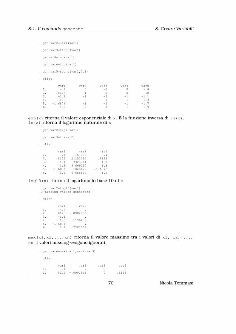
8.1. Il comando generate 8. Creare Variabili
. gen var2=ceil(var1)
. gen var3=floor(var1)
. genvar4=int(var1)
. gen var4=int(var1)
. gen var5=round(var1,0.1)
. clist
var1 var2 var3 var4 var51. -.4 0 -1 0 -.42. .8123 1 0 0 .83. -1.1 -1 -2 -1 -1.14. 1.3 2 1 1 1.35. -1.6876 -1 -2 -1 -1.76. 1.9 2 1 1 1.9
exp(x) ritorna il valore esponenziale di x. È la funzione inversa di ln(x).ln(x) ritorna il logaritmo naturale di x
. gen var2=exp( var1)
. gen var3=ln(var2)
. clist
var1 var2 var31. -.4 .67032 -.42. .8123 2.253084 .81233. -1.1 .3328711 -1.14. 1.3 3.669297 1.35. -1.6876 .1849629 -1.68766. 1.9 6.685894 1.9
log10(x) ritorna il logaritmo in base 10 di x
. gen var2=log10(var1)(3 missing values generated)
. clist
var1 var21. -.4 .2. .8123 -.09028353. -1.1 .4. 1.3 .11394335. -1.6876 .6. 1.9 .2787536
max(x1,x2,...,xn) ritorna il valore massimo tra i valori di x1, x2, ...,xn. I valori missing vengono ignorati.
. gen var4=max(var1,var2,var3)
. clist
var1 var2 var3 var41. -.4 . 2 22. .8123 -.0902835 0 .8123
70 Nicola Tommasi

8. Creare Variabili 8.1. Il comando generate
3. -1.1 . -3 -1.14. 1.3 .1139433 1.31 1.315. -1.6876 . -2.01 -1.68766. 1.9 .2787536 1.5 1.9
min(x1,x2,...,xn) ritorna il valore minimo tra i valori di x1, x2, ..., xn.I valori missing vengono ignorati.
. gen var4=min(var1,var2,var3)
. clist
var1 var2 var3 var41. -.4 . 2 -.42. .8123 -.0902835 0 -.09028353. -1.1 . -3 -34. 1.3 .1139433 1.31 .11394335. -1.6876 . -2.01 -2.016. 1.9 .2787536 1.5 .2787536
sum(x) ritorna la somma incrementale dei valori di x
. gen var3=sum(var1)
. gen var4=sum(var2)
. clist
var1 var2 var3 var41. -.4 . -.4 02. .8123 -.0902835 .4123 -.09028353. -1.1 . -.6877 -.09028354. 1.3 .1139433 .6122999 .02365985. -1.6876 . -1.0753 .02365986. 1.9 .2787536 .8246999 .3024134
8.1.2 Funzioni di distribuzione di probabilità e funzioni di densità
betaden(a,b,x) ritorna la pdf di una distribuzione beta.
. gen var2=betaden(0.1,0.2,var1)
. clist
var1 var21. .4 .23512072. .8123 .31488333. .1 .5919324. .3 .2692645. .6876 .24338556. .9 .4751683
binomial(n,k,p) ritorna le probabilità di una binomiale.
. gen var3=binomial(var1,var2,var0)(1 missing value generated)
. clist
var0 var1 var2 var31. .01 .4 .2351207 1
Nicola Tommasi 71

8.1. Il comando generate 8. Creare Variabili
2. 2.2 .8123 .3148833 .3. .4 3.1 -.591932 04. .6 .3 .269264 15. .8 .6876 .2433855 16. .99 .9 -.4751683 0
chi2(n,x) ritorna la cumulata di una distribuzione chi-quadrato con n gradidi libertà.
. gen var2 = chi2(5,var1)
. clist
var1 var21. .4 .00467042. .8123 .02375783. 3.1 .3154284. .3 .00235695. .6876 .01635776. .9 .0297784
F(n1,n2,f) ritorna la cumulata di una distribuzione F.
. gen var2=F(3,4,var1)
. clist
var1 var21. .4 .2387712. .8123 .45006663. 3.1 .84850154. .3 .17510565. .6876 .39486696. .9 .4849114
Fden(n1,n2,f) ritorna la pdf di una distribuzione F.
. gen var2=Fden(3,4,var1)
. clist
var1 var21. .4 .61496652. .8123 .41526253. 3.1 .06397844. .3 .65570355. .6876 .47113436. .9 .3799204
gammaden(a,b,g,x) ritorna la pdf di una distribuzione Gamma.
. gen var2=gammaden(1,2,0.25,var1)
. clist
var1 var21. .4 .46387172. .8123 .37745753. 3.1 .12025424. .3 .4876555. .6876 .40174126. .9 .3612637
normalden(x,m,s) ritorna la normale con media m e deviazione standard s.
72 Nicola Tommasi

8. Creare Variabili 8.1. Il comando generate
. gen var2=normalden(var1,2,1.5)
. clist
var1 var21. .4 .15057522. .8123 .19439223. 3.1 .20325534. .3 .13992825. .6876 .18138066. .9 .2032553
8.1.3 Funzioni di generazione di numeri random
uniform() ritorna numeri random uniformemente distribuiti nell’intervallo[0,1)
. gen var1=uniform()
. clist
var11. .13698412. .64322073. .55780174. .60479495. .6841766. .1086679
invnormal(uniform()) ritorna numeri random normalmente distribuiti conmedia 0 e deviazione standard 1.
. gen var2=invnormal(uniform())
. clist
var21. .30143382. -1.5459053. .13890864. 1.1332685. -.6583716. -1.700496
8.1.4 Funzioni stringa
abbrev(s,n) ritorna la stringa s abbreviata a n caratteri.
. gen var2=abbrev(var1,5)
. clist
var1 var21. io sono io ~o2. tu sei tu ~i3. egli e´ egl~´4. noi siamo noi~o5. voi siete voi~e6. egli e´ egl~´
length(s) ritorna la lunghezza della stringa s.
Nicola Tommasi 73

8.1. Il comando generate 8. Creare Variabili
var1 var21. io sono 72. tu sei 63. egli e´ 74. noi siamo 95. voi siete 96. egli e´ 7
lower(s), upper(s) ritornano s in lettere minuscole o maiuscole.
gen var2=lower(var1)
. gen var3=upper(var1)
. clist
var1 var2 var31. Io Sono io sono IO SONO2. Tu Sei tu sei TU SEI3. Egli E´ egli e´ EGLI E´4. Noi Siamo noi siamo NOI SIAMO5. Voi Siete voi siete VOI SIETE6. Egli E´ egli e´ EGLI E´
ltrim(s) rtrim(s), trim(s) ritornano s senza spazi iniziali, senza spazifinali o senza spazi all’inizio e alla fine
. gen var2=ltrim(var1)
. gen var3=rtrim(var1)
. gen var4=trim(var1)
. clist
var1 var2 var3 var41. Io Sono Io Sono Io Sono Io Sono2. Tu Sei Tu Sei Tu Sei Tu Sei3. Egli E´ Egli E´ Egli E´ Egli E´4. Noi Siamo Noi Siamo Noi Siamo Noi Siamo5. Voi Siete Voi Siete Voi Siete Voi Siete6. Egli E´ Egli E´ Egli E´ Egli E´
reverse(s) ritorna s invertita.
. gen var2=reverse(var1)
. clist
var1 var21. Io Sono onoS oI2. Tu Sei ieS uT3. Egli E´ ´E ilgE4. Noi Siamo omaiS ioN5. Voi Siete eteiS ioV6. Egli E´ ´E ilgE
strmatch(s1,s2) ritorna 1 se in s1 viene trovato s2, altrimenti ritorna 0.
. gen var2=strmatch( var1,"*E´*")
. clist
var1 var2
74 Nicola Tommasi

8. Creare Variabili 8.1. Il comando generate
1. Io Sono 02. Tu Sei 03. Egli E´ 14. Noi Siamo 05. Voi Siete 06. Egli E´ 1
subinstr(s1,s2,s3,n) in s1 viene sostituito s2 con s3 per le prime n volteche s2 viene trovato. Con il simbolo '.' si sostituiscono tutte le occorrenze dis2 con s.
. gen var2=subinstr(var1,"o","0",.)
. clist
var1 var21. Io Sono I0 S0n02. Tu Sei Tu Sei3. Egli E´ Egli E´4. Noi Siamo N0i Siam05. Voi Siete V0i Siete6. Egli E´ Egli E´
subinword(s1,s2,s3,n) in s1 viene sostituita la parola s2 con la parola s3per le prime n volte che viene trovata. Una parola viene identificata con unospazio bianco. con il simbolo ’.’ si sostituiscono tutte le occorenze di s2 cons3.
. gen var2=subinword(var1,"E´","&",.)
. clist
var1 var21. Io Sono Io Sono2. Tu Sei Tu Sei3. Egli E´ Egli &4. Noi Siamo Noi Siamo5. Voi Siete Voi Siete6. Egli E´ Egli &
substr(s,n1,n2) ritorna la stringa di s che parte dalla posizione n1 fino allaposizione n2. Se n1 è un valore negativo vuol dire che si parte a contare dallafine della stringa s.
. gen var2=substr(var1,3,3)
. clist
var1 var21. Io Sono So2. Tu Sei Se3. Egli E´ li4. Noi Siamo i S5. Voi Siete i S6. Egli E´ li
word(s,n) ritorna la n-esima parola all’interno della stringa s.
. gen var2=word(var1,1)
. clist
Nicola Tommasi 75

8.1. Il comando generate 8. Creare Variabili
var1 var21. Io Sono Io2. Tu Sei Tu3. Egli E´ Egli4. Noi Siamo Noi5. Voi Siete Voi6. Egli E´ Egli
wordcount(s) conta il numero di parole all’interno della stringa s.
. gen var2=wordcount(var1)
. clist
var1 var21. Io Sono 22. Tu Sei 23. Egli E´ 24. Noi Siamo 25. Voi Siete 26. Egli E´ 2
8.1.5 Funzioni di programmazione
inlist(z,a,b,...) ritorna 1 se il contenuto di z è presente in uno degli argo-menti successivi, altrimenti ritorna 0. Gli argomenti possono essere numericio stringa. Se sono numerici possono essere in un numero tra 2 e 255, se sonostringa tra 2 e 10.
. gen cod_com=.;(395 missing values generated)
. replace cod_com=2 if inlist(q03,"affi");(0 real changes made)
. replace cod_com=2 if inlist(q03,"gazzo v.se");(0 real changes made)
. replace cod_com=6 if inlist(q03,"bardolino","cisano bardolino");(2 real changes made)
(output omitted )
. replace cod_com=96 if inlist(q03,"alpo villafranca","s.ambrogio di villa vr",> "villafranca","villafranca di vr");(2 real changes made)
. replace cod_com=97 if inlist(q03,"zevio","zevio vr");(2 real changes made)
cond(x,a,b,c) o cond(x,a,b) ritorna a se x è vero, b se x è falso e c se x èmissing. Se c non è specificato allora in x viene messo valore missing.
. clist
var1 var21. 1 12. 1 23. 2 1
76 Nicola Tommasi
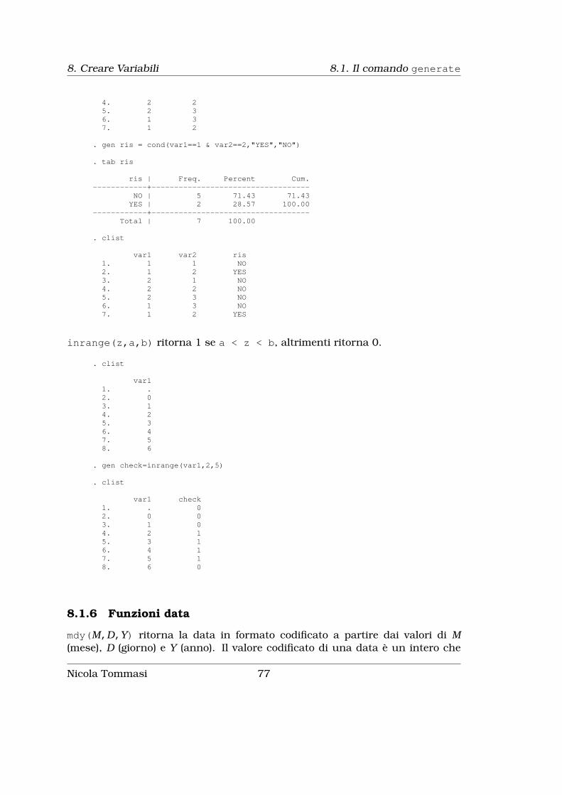
8. Creare Variabili 8.1. Il comando generate
4. 2 25. 2 36. 1 37. 1 2
. gen ris = cond(var1==1 & var2==2,"YES","NO")
. tab ris
ris | Freq. Percent Cum.------------+-----------------------------------
NO | 5 71.43 71.43YES | 2 28.57 100.00
------------+-----------------------------------Total | 7 100.00
. clist
var1 var2 ris1. 1 1 NO2. 1 2 YES3. 2 1 NO4. 2 2 NO5. 2 3 NO6. 1 3 NO7. 1 2 YES
inrange(z,a,b) ritorna 1 se a < z < b, altrimenti ritorna 0.
. clist
var11. .2. 03. 14. 25. 36. 47. 58. 6
. gen check=inrange(var1,2,5)
. clist
var1 check1. . 02. 0 03. 1 04. 2 15. 3 16. 4 17. 5 18. 6 0
8.1.6 Funzioni data
mdy(M,D,Y) ritorna la data in formato codificato a partire dai valori di M(mese), D (giorno) e Y (anno). Il valore codificato di una data è un intero che
Nicola Tommasi 77

8.1. Il comando generate 8. Creare Variabili
identifica il giorno a partire dalla data del 01 gennaio 1960 (01 gennaio 1960=1,01 gennaio 1960=2 e così via).
. summ month day year
Variable | Obs Mean Std. Dev. Min Max-------------+--------------------------------------------------------
month | 1652 9.214891 3.134451 1 12day | 1652 16.77421 8.470449 1 31
year | 1651 2005.998 .0491769 2005 2006
. clist month day year in 1/7
month day year1. . . .2. 9 8 20063. 10 29 20064. 11 28 20065. 12 3 20066. 10 10 20067. 10 26 2006
. gen comp = mdy(month,day,year)(690 missing values generated)
. clist month day year comp in 1/7
month day year comp1. . . . .2. 9 8 2006 170523. 10 29 2006 171034. 11 28 2006 171335. 12 3 2006 171386. 10 10 2006 170847. 10 26 2006 17100
. format comp %dd/N/CY
. clist month day year comp in 1/7
month day year comp1. . . . .2. 9 8 2006 8/09/20063. 10 29 2006 29/10/20064. 11 28 2006 28/11/20065. 12 3 2006 3/12/20066. 10 10 2006 10/10/20067. 10 26 2006 26/10/2006
8.1.7 Funzioni per serie temporali
. . .
8.1.8 Funzioni matriciali
diag(v) ritorna la matrice quadrata diagonale costruita a partire dal vettorev.
78 Nicola Tommasi

8. Creare Variabili 8.1. Il comando generate
. matrix list Y
Y[1,4]c1 c2 c3 c4
r1 1 2 3 4
. matrix Ydiag=diag(Y)
. matrix list Ydiag
symmetric Ydiag[4,4]c1 c2 c3 c4
c1 1c2 0 2c3 0 0 3c4 0 0 0 4
. matrix list X
X[4,1]c1
r1 1r2 2r3 3r4 4
. matrix Xdiag=diag(X)
. matrix list Xdiag
symmetric Xdiag[4,4]r1 r2 r3 r4
r1 1r2 0 2r3 0 0 3r4 0 0 0 4
inv(M) ritorna l’inversa della matrice M.
. matrix list X
X[4,4]c1 c2 c3 c4
r1 .1 .2 .3 .4r2 .5 .6 .7 .8r3 .9 .094 .11 .12r4 .13 .14 .15 .16
. matrix Xinv = inv(X)
. matrix list Xinv
Xinv[4,4]r1 r2 r3 r4
c1 2.697e+13 -4.046e+13 1.233951 1.349e+14c2 3.641e+15 -5.462e+15 -.08328654 1.821e+16c3 -7.364e+15 1.105e+16 -3.5352798 -3.682e+16c4 3.695e+15 -5.543e+15 2.3846154 1.848e+16
colsof(M) ritorna uno scalare con il numero di righe della matrice M; rowsof(M)ritorna uno scalare con il numero di colonne della matrice M.
Nicola Tommasi 79
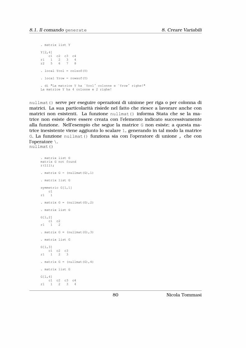
8.1. Il comando generate 8. Creare Variabili
. matrix list Y
Y[2,4]c1 c2 c3 c4
r1 1 2 3 4r2 5 6 7 8
. local Ycol = colsof(Y)
. local Yrow = rowsof(Y)
. di "La matrice Y ha `Ycol´ colonne e `Yrow´ righe!"La matrice Y ha 4 colonne e 2 righe!
nullmat() serve per eseguire operazioni di uinione per riga o per colonna dimatrici. La sua particolarità risiede nel fatto che riesce a lavorare anche conmatrici non esistenti. La funzione nullmat() informa Stata che se la ma-trice non esiste deve essere creata con l’elemento indicato successivamentealla funzione. Nell’esempio che segue la matrice G non esiste; a questa ma-trice inesistente viene aggiunto lo scalare 1, generando in tal modo la matriceG. La funzione nullmat() funziona sia con l’operatore di unione , che conl’operatore \.nullmat()
. matrix list Gmatrix G not foundr(111);
. matrix G = (nullmat(G),1)
. matrix list G
symmetric G[1,1]c1
r1 1
. matrix G = (nullmat(G),2)
. matrix list G
G[1,2]c1 c2
r1 1 2
. matrix G = (nullmat(G),3)
. matrix list G
G[1,3]c1 c2 c3
r1 1 2 3
. matrix G = (nullmat(G),4)
. matrix list G
G[1,4]c1 c2 c3 c4
r1 1 2 3 4
80 Nicola Tommasi
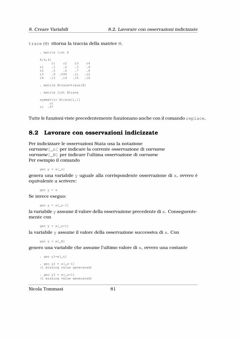
8. Creare Variabili 8.2. Lavorare con osservazioni indicizzate
trace(M) ritorna la traccia della matrice M.
. matrix list X
X[4,4]c1 c2 c3 c4
r1 .1 .2 .3 .4r2 .5 .6 .7 .8r3 .9 .094 .11 .12r4 .13 .14 .15 .16
. matrix Xtrace=trace(X)
. matrix list Xtrace
symmetric Xtrace[1,1]c1
r1 .97
Tutte le funzioni viste precedentemente funzionano anche con il comando replace.
8.2 Lavorare con osservazioni indicizzate
Per indicizzare le osservazioni Stata usa la notazionevarname[_n] per indicare la corrente osservazione di varnamevarname[_N] per indicare l’ultima osservazione di varnamePer esempio il comando
gen y = x[_n]
genera una variabile y uguale alla corrispondente osservazione di x, ovvero èequivalente a scrivere:
gen y = x
Se invece eseguo:
gen y = x[_n-1]
la variabile y assume il valore della osservazione precedente di x. Conseguente-mente con
gen y = x[_n+1]
la variabile y assume il valore della osservazione successiva di x. Con
gen y = x[_N]
genero una variabile che assume l’ultimo valore di x, ovvero una costante
. gen y1=x[_n]
. gen y2 = x[_n-1](1 missing value generated)
. gen y3 = x[_n+1](1 missing value generated)
Nicola Tommasi 81

8.2. Lavorare con osservazioni indicizzate 8. Creare Variabili
. gen y4 = x[_N]
. clist
x y1 y2 y3 y41. 1 1 . 2 62. 2 2 1 3 63. 3 3 2 4 64. 4 4 3 5 65. 5 5 4 6 66. 6 6 5 . 6
Utile per creare velocemente una variabile chiave o indice è il comando
gen ID = _n
che crea una successione con passo 1 dalla prima all’ultima osservazione,secondo l’ordinamento corrente delle osservazioniInfine con la costruzione:
gen y = x[_N-_n+1]
genero y in ordine inverso di x.
. gen ID = _n
. gen y = ID[_N-_n+1]
. clist nquest nord eta ID y
nquest nord eta ID y1. 34 1 59 1 102. 34 2 58 2 93. 34 3 31 3 84. 34 4 29 4 75. 173 1 54 5 66. 173 2 52 6 57. 173 3 27 7 48. 173 4 24 8 39. 375 1 77 9 210. 375 2 76 10 1
Naturalmente possiamo ricorrere anche al prefisso by. Per esempio
sort fam_id agebysort fam_id: gen old = age[_N]
genera una variabile con l’età più alta per ciascun fam_id
. sort nquest eta
. bysort nquest: gen old = eta[_N]
. clist nquest eta old
nquest eta old1. 34 29 592. 34 31 593. 34 58 594. 34 59 595. 173 24 546. 173 27 54
82 Nicola Tommasi
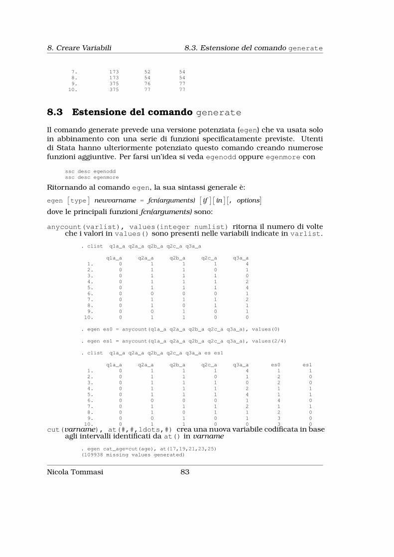
8. Creare Variabili 8.3. Estensione del comando generate
7. 173 52 548. 173 54 549. 375 76 7710. 375 77 77
8.3 Estensione del comando generate
Il comando generate prevede una versione potenziata (egen) che va usata soloin abbinamento con una serie di funzioni specificatamente previste. Utentidi Stata hanno ulteriormente potenziato questo comando creando numerosefunzioni aggiuntive. Per farsi un’idea si veda egenodd oppure egenmore con
ssc desc egenoddssc desc egenmore
Ritornando al comando egen, la sua sintassi generale è:
egen[type
]newvarname = fcn(arguments)
[if
][in
][, options
]dove le principali funzioni fcn(arguments) sono:
anycount(varlist), values(integer numlist) ritorna il numero di volteche i valori in values() sono presenti nelle variabili indicate in varlist.
. clist q1a_a q2a_a q2b_a q2c_a q3a_a
q1a_a q2a_a q2b_a q2c_a q3a_a1. 0 1 1 1 42. 0 1 1 0 13. 0 1 1 1 04. 0 1 1 1 25. 0 1 1 1 46. 0 0 0 0 17. 0 1 1 1 28. 0 1 0 1 19. 0 0 1 0 110. 0 1 1 0 0
. egen es0 = anycount(q1a_a q2a_a q2b_a q2c_a q3a_a), values(0)
. egen es1 = anycount(q1a_a q2a_a q2b_a q2c_a q3a_a), values(2/4)
. clist q1a_a q2a_a q2b_a q2c_a q3a_a es es1
q1a_a q2a_a q2b_a q2c_a q3a_a es0 es11. 0 1 1 1 4 1 12. 0 1 1 0 1 2 03. 0 1 1 1 0 2 04. 0 1 1 1 2 1 15. 0 1 1 1 4 1 16. 0 0 0 0 1 4 07. 0 1 1 1 2 1 18. 0 1 0 1 1 2 09. 0 0 1 0 1 3 010. 0 1 1 0 0 3 0
cut(varname), at(#,#,ldots,#) crea una nuova variabile codificata in baseagli intervalli identificati da at() in varname
. egen cat_age=cut(age), at(17,19,21,23,25)(109938 missing values generated)
Nicola Tommasi 83

8.3. Estensione del comando generate 8. Creare Variabili
. tab age cat_age
| cat_ageAge ind | 17 19 21 23 | Total
-----------+--------------------------------------------+----------17 | 2,044 0 0 0 | 2,04418 | 2,199 0 0 0 | 2,19919 | 0 2,270 0 0 | 2,27020 | 0 2,388 0 0 | 2,38821 | 0 0 2,477 0 | 2,47722 | 0 0 2,546 0 | 2,54623 | 0 0 0 2,593 | 2,59324 | 0 0 0 2,696 | 2,696
-----------+--------------------------------------------+----------Total | 4,243 4,658 5,023 5,289 | 19,213
max(exp) ritorna una variabile (costante) con il valore massimo assunto dallevariabili elencate in exp.
. clist foreign price
foreign price1. Foreign 4,4992. Foreign 6,2293. Domestic 4,9344. Domestic 3,6675. Domestic 4,1726. Foreign 8,1297. Foreign 4,5898. Domestic 3,9849. Foreign 5,07910. Domestic 6,486
. egen es = max(price), by(foreign)
. clist foreign price es
foreign price es1. Foreign 4,499 81292. Foreign 6,229 81293. Domestic 4,934 64864. Domestic 3,667 64865. Domestic 4,172 64866. Foreign 8,129 81297. Foreign 4,589 81298. Domestic 3,984 64869. Foreign 5,079 812910. Domestic 6,486 6486
mean(exp) ritorna una variabile (costante) con il valore medio delle variabilielencate in exp.
. clist foreign price
foreign price1. Foreign 4,4992. Foreign 6,2293. Domestic 4,9344. Domestic 3,6675. Domestic 4,1726. Foreign 8,1297. Foreign 4,5898. Domestic 3,9849. Foreign 5,07910. Domestic 6,486
84 Nicola Tommasi

8. Creare Variabili 8.3. Estensione del comando generate
. egen es0=mean(price)
. egen es1=mean(price), by(foreign)
. clist foreign price es?
foreign price es0 es11. Foreign 4,499 5176.8 57052. Foreign 6,229 5176.8 57053. Domestic 4,934 5176.8 4648.64. Domestic 3,667 5176.8 4648.65. Domestic 4,172 5176.8 4648.66. Foreign 8,129 5176.8 57057. Foreign 4,589 5176.8 57058. Domestic 3,984 5176.8 4648.69. Foreign 5,079 5176.8 570510. Domestic 6,486 5176.8 4648.6
median(exp) ritorna una variabile (costante) con il valore mediano delle vari-abili elencate in exp.
. clist q3?_a
q3a_a q3b_a q3c_a q3d_a1. 4 1 0 02. 1 0 0 03. 0 0 0 04. 2 0 0 05. 4 4 3 16. 1 0 0 07. 2 2 0 08. 1 0 0 09. 1 0 0 010. 0 1 0 0
. egen es0=median(q3a_a)
. egen es2=median(q3a_a-q3d_a)
. clist q3?_a es?
q3a_a q3b_a q3c_a q3d_a es1 es0 es21. 4 1 0 0 1 1 12. 1 0 0 0 0 1 13. 0 0 0 0 0 1 14. 2 0 0 0 1 1 15. 4 4 3 1 1 1 16. 1 0 0 0 0 1 17. 2 2 0 0 1 1 18. 1 0 0 0 0 1 19. 1 0 0 0 0 1 110. 0 1 0 0 0 1 1
min(exp) ritorna una variabile (costante) con il valore minimo delle variabilielencate in exp.
. clist foreign length
foreign length 1. Foreign 149 2. Foreign 170 3. Domestic 198
4. Domestic 179 5. Domestic 179 6. Foreign 184 7. Foreign 165
8. Domestic 163 9. Foreign 170 10. Domestic 182
. egen es0=min(length)
Nicola Tommasi 85

8.4. Sostituire valori in una variabile 8. Creare Variabili
. egen es1=min(length), by( foreign)
. clist foreign length es?
foreign length es0 es1 1. Foreign 149 149 149 2. Foreign 170
149 149 3. Domestic 198 149 163 4. Domestic 179 149 163 5.
Domestic 179 149 163 6. Foreign 184 149 149 7. Foreign 165 149
149 8. Domestic 163 149 163 9. Foreign 170 149 149 10.
Domestic 182 149 163
mode(varname) [, minmode maxmode nummode(integer) missing] ritornauna variabile (costante) con il valore della moda delle variabili elencatein varname. Se esistono più valori modali, con l’opzione minmode sisceglie il minore, con maxmode il maggiore, con nummode(integer) lamoda n-esima espressa da integer.
rowmax(varlist) ritorna il valore massimo per ciascuna osservazione tra i val-ori delle variabili elencate in varlist.
rowmean(varlist) ritorna il valore medio per ciascuna osservazione dei valoridelle variabili elencate in varlist.
rowmin(varlist) ritorna il valore minimo per ciascuna osservazione tra i valoridelle variabili elencate in varlist.
rowmiss(varlist) ritorna il numero di valori missing per ciascuna osservazionetra i valori delle variabili elencate in varlist.
rownonmiss(varlist) ritorna il numero di valori non missing per ciascunaosservazione tra i valori delle variabili elencate in varlist.
rowsd(varlist) ritorna la deviazione standard per ciascuna osservazione dei ivalori delle variabili elencate in varlist.
sum(exp) conta quante osservazioni rispondono al criterio exp.
8.4 Sostituire valori in una variabile
Il comando principale per sostituire dei valori secondo una certa funzione è
replace oldvar =exp[if
][in
]che può essere usato anche con variabili stringa avendo l’accortezza di racchi-udere il valore da sostituire tra virgolette:
replace str_var = "stringa" if....
Se i valori da considerare sono molti e sono relativi ad una stessa variabile,anziché ricorrere ad una lunga serie di replace condizionati, è possibile usarela funzione inlist che abbiamo visto tra le funzioni di programmazione delcomando generate
. gen macro1=1 if inlist(regione,1,2,3,7,4,5,6,8);(43456 missing values generated)
86 Nicola Tommasi

8. Creare Variabili 8.4. Sostituire valori in una variabile
. replace macro1=2 if inlist(regione,9,10,11,12);(13891 real changes made)
. replace macro1=3 if inlist(regione,13,14,15,16,17,18,19,20);(29565 real changes made)
. tab regione macro1, miss nolab;
| macro1Regione | 1 2 3 | Total
-----------+---------------------------------+----------1 | 4,714 0 0 | 4,7142 | 1,526 0 0 | 1,5263 | 8,166 0 0 | 8,1664 | 3,705 0 0 | 3,7055 | 4,994 0 0 | 4,9946 | 2,029 0 0 | 2,0297 | 2,322 0 0 | 2,3228 | 3,968 0 0 | 3,9689 | 0 4,236 0 | 4,23610 | 0 2,265 0 | 2,26511 | 0 2,931 0 | 2,93112 | 0 4,459 0 | 4,45913 | 0 0 2,653 | 2,65314 | 0 0 1,972 | 1,97215 | 0 0 6,018 | 6,01816 | 0 0 4,963 | 4,96317 | 0 0 2,225 | 2,22518 | 0 0 3,454 | 3,45419 | 0 0 5,426 | 5,42620 | 0 0 2,854 | 2,854
-----------+---------------------------------+----------Total | 31,424 13,891 29,565 | 74,880
Altro importante comando è recode che consente di ricodificare i valori di unavariabile (o più variabili) secondo certi criteri (erule) e che prevede numerosepossibilità:
recode varlist(erule)[(erule) ...
][if
][in
][, options
]Almeno una regola di ricodifica deve essere definita e può assumere le seguentiformeRegola Esempio Esito(# = #) (8 = 4) Trasforma tutti i valori 8 in 4#1 #2 = #) (8 7 = 4) Trasforma tutti i valori 8 e 7 in 4#1 / #2 = #) (1/8=4) Trasforma tutti i valori da 1 a 8 (compresi) in 4nonmissing = # (nonmissing = 4) Trasforma tutti i valori non missing in 4missing = # (missing=9) Trasforma tutti i valori missing in 9#/max 5/max=5 Trasforma tutti i valori superiori a 5 in 5min/# min/8=8 Trasforma tutti i valori inferiori a 8 in 8
Le variabili a cui applicare la trasformazione possono essere più di una. Senon viene specificata nessuna opzione del tipo generate o prefix, la sosti-tuzione avviene direttamente nelle variabili di varlist. Se invece si voglionocreare nuove variabili che contengano la ricodifica si ricorrerà all’opzione
Nicola Tommasi 87
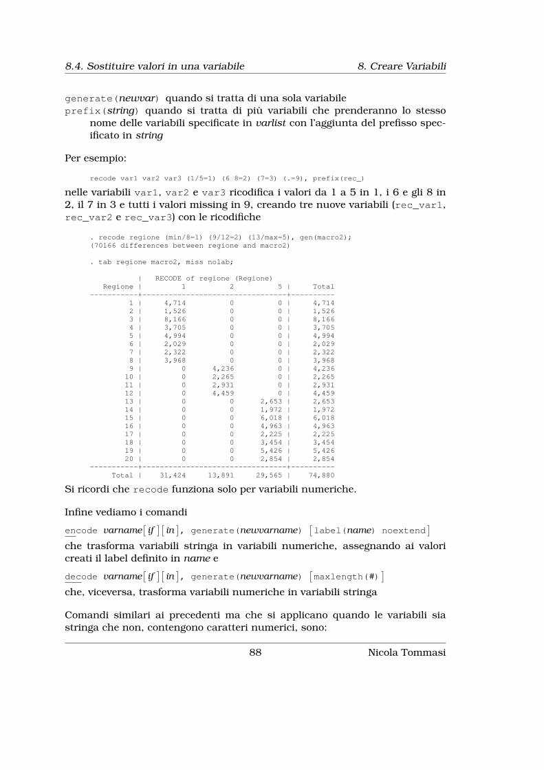
8.4. Sostituire valori in una variabile 8. Creare Variabili
generate(newvar) quando si tratta di una sola variabileprefix(string) quando si tratta di più variabili che prenderanno lo stesso
nome delle variabili specificate in varlist con l’aggiunta del prefisso spec-ificato in string
Per esempio:
recode var1 var2 var3 (1/5=1) (6 8=2) (7=3) (.=9), prefix(rec_)
nelle variabili var1, var2 e var3 ricodifica i valori da 1 a 5 in 1, i 6 e gli 8 in2, il 7 in 3 e tutti i valori missing in 9, creando tre nuove variabili (rec_var1,rec_var2 e rec_var3) con le ricodifiche
. recode regione (min/8=1) (9/12=2) (13/max=5), gen(macro2);(70166 differences between regione and macro2)
. tab regione macro2, miss nolab;
| RECODE of regione (Regione)Regione | 1 2 5 | Total
-----------+---------------------------------+----------1 | 4,714 0 0 | 4,7142 | 1,526 0 0 | 1,5263 | 8,166 0 0 | 8,1664 | 3,705 0 0 | 3,7055 | 4,994 0 0 | 4,9946 | 2,029 0 0 | 2,0297 | 2,322 0 0 | 2,3228 | 3,968 0 0 | 3,9689 | 0 4,236 0 | 4,23610 | 0 2,265 0 | 2,26511 | 0 2,931 0 | 2,93112 | 0 4,459 0 | 4,45913 | 0 0 2,653 | 2,65314 | 0 0 1,972 | 1,97215 | 0 0 6,018 | 6,01816 | 0 0 4,963 | 4,96317 | 0 0 2,225 | 2,22518 | 0 0 3,454 | 3,45419 | 0 0 5,426 | 5,42620 | 0 0 2,854 | 2,854
-----------+---------------------------------+----------Total | 31,424 13,891 29,565 | 74,880
Si ricordi che recode funziona solo per variabili numeriche.
Infine vediamo i comandi
encode varname[if
][in
], generate(newvarname)
[label(name) noextend
]che trasforma variabili stringa in variabili numeriche, assegnando ai valoricreati il label definito in name e
decode varname[if
][in
], generate(newvarname)
[maxlength(#)
]che, viceversa, trasforma variabili numeriche in variabili stringa
Comandi similari ai precedenti ma che si applicano quando le variabili siastringa che non, contengono caratteri numerici, sono:
88 Nicola Tommasi

8. Creare Variabili 8.4. Sostituire valori in una variabile
destring[varlist
], {generate(newvarlist)|replace}
[destring_options
]che converte variabili numeriche stringa in numeriche pure. Con l’opzioneignore("chars") si possono specificare caratteri non numerici da rimuovere.Nell’esempio che segue abbiamo la variabile stringa balance che contiene siadati numerici che stringa. Per poterla rendere numerica per prima cosa siprovvederà a convertire i dati stringa in missing (.a e .b) e poi si applicherà ilcomando destring
. desc balance;storage display value
variable name type format label variable label------------------------------------------------------------balance str8 %9s
tab balance, miss;balance | Freq. Percent Cum.
------------+-----------------------------------1112.99 | 1 6.67 6.671397.99 | 1 6.67 13.33
16.11 | 1 6.67 20.002177.22 | 1 6.67 26.672371.62 | 1 6.67 33.332517.15 | 1 6.67 40.00273.91 | 1 6.67 46.672751.6 | 1 6.67 53.33
INS Paid | 4 26.67 80.00NULL | 3 20.00 100.00
------------+-----------------------------------Total | 15 100.00
. destring balance, replace;balance contains non-numeric characters; no replace
. replace balance =".a" if balance=="INS Paid";(4 real changes made)
. replace balance =".b" if balance=="NULL";(3 real changes made)
. destring balance, replace;balance has all characters numeric; replaced as double(7 missing values generated)
. summ balance;Variable | Obs Mean Std. Dev. Min Max
-------------+--------------------------------------------------------balance | 8 1577.324 1044.511 16.11 2751.6
. desc balance;storage display value
variable name type format label variable label----------------------------------------------------------------------balance double %10.0g
Il comando tostring, viceversa converte variabili numeriche in variabili stringa
tostring varlist, {generate(newvarlist)|replace}[tostring_options
]. desc eta
Nicola Tommasi 89

8.5. Creare variabili dummy 8. Creare Variabili
storage display valuevariable name type format label variable label----------------------------------------------------------------------eta int %10.0g
. summ eta
Variable | Obs Mean Std. Dev. Min Max-------------+--------------------------------------------------------
eta | 74880 41.71912 22.25459 0 102
. tostring eta, replaceeta was int now str3
. desc eta
storage display valuevariable name type format label variable label----------------------------------------------------------------------eta str3 %9s
. summ eta
Variable | Obs Mean Std. Dev. Min Max-------------+--------------------------------------------------------
eta | 0
. destring eta, replaceeta has all characters numeric; replaced as int
. desc eta
storage display valuevariable name type format label variable label----------------------------------------------------------------------eta int %10.0g
. summ eta
Variable | Obs Mean Std. Dev. Min Max-------------+--------------------------------------------------------
eta | 74880 41.71912 22.25459 0 102
8.5 Creare variabili dummy
Le variabili dummy sono variabili che assumo valori 0 e 1. In particolare 1quando la caratteristica in esame è presente, 0 quando è assente. Vediamoadesso due metodi per creare questo tipo di variabili. Il primo sistema si basasulla tecnica del replace; si crea una variabile ponedola pari a 0 e poi sisotituisce il valore 1 secondo un certo criterio:
. gen nord=0
. replace nord=1 if ripgeo==1 | ripgeo==2(61098 real changes made)
. tab nord, miss
90 Nicola Tommasi

8. Creare Variabili 8.5. Creare variabili dummy
nord | Freq. Percent Cum.------------+-----------------------------------
0 | 78,925 56.37 56.371 | 61,098 43.63 100.00
------------+-----------------------------------Total | 140,023 100.00
Oppure in maniera meno pedante
. gen north = ripgeo<=2
. tab nord, miss
nord | Freq. Percent Cum.------------+-----------------------------------
0 | 78,925 56.37 56.371 | 61,098 43.63 100.00
------------+-----------------------------------Total | 140,023 100.00
Con il secondo metodo si sfrutta l’opzione gen del comando tabulate
. tab ripgeo, miss gen(ripgeo_)
ripgeo | Freq. Percent Cum.------------+-----------------------------------
1 | 32,188 22.99 22.992 | 28,910 20.65 43.633 | 26,768 19.12 62.754 | 37,206 26.57 89.325 | 14,951 10.68 100.00
------------+-----------------------------------Total | 140,023 100.00
. tab1 ripgeo_*
-> tabulation of ripgeo_1
ripgeo== |1.0000 | Freq. Percent Cum.
------------+-----------------------------------0 | 107,835 77.01 77.011 | 32,188 22.99 100.00
------------+-----------------------------------Total | 140,023 100.00
-> tabulation of ripgeo_2
ripgeo== |2.0000 | Freq. Percent Cum.
------------+-----------------------------------0 | 111,113 79.35 79.351 | 28,910 20.65 100.00
------------+-----------------------------------Total | 140,023 100.00
-> tabulation of ripgeo_3
ripgeo== |3.0000 | Freq. Percent Cum.
------------+-----------------------------------0 | 113,255 80.88 80.881 | 26,768 19.12 100.00
------------+-----------------------------------Total | 140,023 100.00
Nicola Tommasi 91

8.5. Creare variabili dummy 8. Creare Variabili
-> tabulation of ripgeo_4
ripgeo== |4.0000 | Freq. Percent Cum.
------------+-----------------------------------0 | 102,817 73.43 73.431 | 37,206 26.57 100.00
------------+-----------------------------------Total | 140,023 100.00
-> tabulation of ripgeo_5
ripgeo== |5.0000 | Freq. Percent Cum.
------------+-----------------------------------0 | 125,072 89.32 89.321 | 14,951 10.68 100.00
------------+-----------------------------------Total | 140,023 100.00
. summ ripgeo_*
Variable | Obs Mean Std. Dev. Min Max-------------+--------------------------------------------------------
ripgeo_1 | 140023 .2298765 .4207548 0 1ripgeo_2 | 140023 .2064661 .4047703 0 1ripgeo_3 | 140023 .1911686 .3932229 0 1ripgeo_4 | 140023 .2657135 .441714 0 1ripgeo_5 | 140023 .1067753 .3088285 0 1
Si noti che la media delle variabili dummy corrisponde alla percentuale di valori1.
92 Nicola Tommasi

Capitolo 9
Analisi Quantitativa
9.1 summarize e tabulate
Per prima cosa è bene distinguere le analisi da condurre su variabili continuee quelle su variabili discrete. Per le prime il comando essenziale è:
summarize[varlist
][if
][in
][weight
][, detail
]dove detail produce un output con un numero maggiore di informazioni.Inoltre questo comando supporta l’uso dei pesi (
[weight
]) che possono essere
uno tra aweight, fweight e iweight e servono per produrre delle statistichepesate.
. summ y1 yt, detail
Reddito disponibile netto-------------------------------------------------------------
Percentiles Smallest1% 3600 05% 12050 010% 17000 0 Obs 800125% 27200 0 Sum of Wgt. 8001
50% 42600 Mean 51212.38Largest Std. Dev. 38811.92
75% 65964 557239.390% 92000 630000.8 Variance 1.51e+0995% 114100 764335.5 Skewness 4.34293499% 188500 800000 Kurtosis 52.93251
Reddito da pensioni e altri trasferimenti-------------------------------------------------------------
Percentiles Smallest1% 0 05% 0 010% 0 0 Obs 800125% 0 0 Sum of Wgt. 8001
50% 8840 Mean 12683.57Largest Std. Dev. 15618.38
75% 22100 12785090% 32500 139300 Variance 2.44e+08
93

9.1. summarize e tabulate 9. Analisi Quantitativa
95% 41223 150800 Skewness 1.62405999% 65000 169000 Kurtosis 7.892386
. summ y1 yt [aweight=pesofit]
Variable | Obs Weight Mean Std. Dev. Min Max---------+--------------------------------------------------------------
y1 | 8001 8001 49152.49 36364.71 0 800000yt | 8001 8001 11932.83 14946.91 0 169000
Un comando aggiuntivo simile ma che offre una gamma più ampia di possibil-ità è fsum.
. fsum y1 yt, f(10.3) s(n abspct miss mean median sum)
Variable | N Missing AbsPct Mean Median Sum----------+------------------------------------------------------------
y1 | 8001 0 0.000 51212.380 42600.000 4.098e+08yt | 8001 0 0.000 12683.571 8840.000 1.015e+08
. fsum y1 yt, f(10.3) s(n miss mean median sum) uselabel
Variable | N Missing Mean Median Sum------------------------------+----------------------------------------
Reddito disponibile netto | 8001 0 51212.3 42600.0 4.098e+08Reddito da pens e altri trasf | 8001 0 12683.5 8840.0 1.015e+08
Per le variabili discrete il comando principale è tabulate che analizzeremo nelcaso di analisi di una sola variabile e nel caso di incrocio tra due variabili.Nel caso si voglia analizzare la distribuzione di frequenza di una sola variabilediscreta il comando è:
tabulate varname[if
][in
][weight
][, tabulate_options
]tra le tabulate_options più importanti:
missing per includere anche le osservazioni missingnolabel per visualizzare i codici numerici al posto delle etichette dei valorisort per ordinare in senso discendente in base alla frequenza delle diverse
specificazioni della variabilesum(var) per fare il sum di una variabile continua per ciascuna specificazione
di varname
. tab d09a
Chiarezza della |segnaletica | Freq. Percent Cum.
--------------------------+-----------------------------------Per nulla soddisfatto | 12 0.55 0.55
Poco soddisfatto | 46 2.11 2.67Soddisfatto | 733 33.70 36.37
Più che Soddisfatto | 563 25.89 62.25Completamente Soddisfatto | 795 36.55 98.80
Non saprei | 26 1.20 100.00--------------------------+-----------------------------------
Total | 2,175 100.00
94 Nicola Tommasi

9. Analisi Quantitativa 9.1. summarize e tabulate
. tab d09a, miss
Chiarezza della |segnaletica | Freq. Percent Cum.
--------------------------+-----------------------------------Per nulla soddisfatto | 12 0.51 0.51
Poco soddisfatto | 46 1.96 2.48Soddisfatto | 733 31.31 33.79
Più che Soddisfatto | 563 24.05 57.84Completamente Soddisfatto | 795 33.96 91.80
Non saprei | 26 1.11 92.91Non risponde | 166 7.09 100.00
--------------------------+-----------------------------------Total | 2,341 100.00
. tab d09a, miss nolab
Chiarezza |della |
segnaletica | Freq. Percent Cum.------------+-----------------------------------
1 | 12 0.51 0.512 | 46 1.96 2.483 | 733 31.31 33.794 | 563 24.05 57.845 | 795 33.96 91.806 | 26 1.11 92.91.a | 166 7.09 100.00
------------+-----------------------------------Total | 2,341 100.00
. tab d09a, miss nolab sort
Chiarezza |della |
segnaletica | Freq. Percent Cum.------------+-----------------------------------
5 | 795 33.96 33.963 | 733 31.31 65.274 | 563 24.05 89.32.a | 166 7.09 96.412 | 46 1.96 98.386 | 26 1.11 99.491 | 12 0.51 100.00
------------+-----------------------------------Total | 2,341 100.00
. tab d09a, miss nolab sum(d01)
Chiarezza |della | Summary of Età
segnaletica | Mean Std. Dev. Freq.------------+------------------------------------
1 | 51.363636 21.795746 112 | 48.369565 18.587162 463 | 51.283727 19.146486 7194 | 51.70991 18.997164 5555 | 53.497409 18.69334 7726 | 42.375 17.392683 24.a | 63.362416 15.511641 149
------------+------------------------------------Total | 52.776801 18.965238 2276
Nicola Tommasi 95

9.1. summarize e tabulate 9. Analisi Quantitativa
Sempre nel caso di analisi di frequenza univariata segnalo il comando aggiun-tivo fre che consente, tra l’altro, di di esportare i risultati anche in Tex:
fre[varlist
][if
][in
][weight
][, options
]Tra le options citiamo:
format(#) che indica il numero di decimali (2 è il valore di default)nomissing omette dalla tabella il conteggio dei valori missingnolabel omette il label delle variabilinovalue omette il valore numerico delle labelnoname omette il nome della variabilenotitle omette il titolo con il nome e la descrizione della variabilenowrap non manda a capo l’intestazione di rigawidth(#) specifica la larghezza della colonna delle descrizioniinclude include tutti i valori possibili della variabile, quindi comprende anche
quelli a frequenza zeroinclude(numlist) include solo i valori specificati in numlistascending visualizza i valori in ordine ascendente di frequenzadescending visualizza i valori in ordine discendente di frequenza
. fre d09a
d09a -- Chiarezza della segnaletica----------------------------------------------------------------------------------
| Freq. Percent Valid Cum.-------------------------------------+--------------------------------------------Valid 1 Per nulla soddisfatto | 12 0.51 0.55 0.55
2 Poco soddisfatto | 46 1.96 2.11 2.673 Soddisfatto | 733 31.31 33.70 36.374 Più che Soddisfatto | 563 24.05 25.89 62.255 Completamente Soddisfatto | 795 33.96 36.55 98.806 Non saprei | 26 1.11 1.20 100.00Total | 2175 92.91 100.00
Missing .a Non risponde | 166 7.09Total | 2341 100.00----------------------------------------------------------------------------------
. fre d09a, nomissing
d09a -- Chiarezza della segnaletica---------------------------------------------------------------
| Freq. Percent Cum.-----------------------------+---------------------------------1 Per nulla soddisfatto | 12 0.55 0.552 Poco soddisfatto | 46 2.11 2.673 Soddisfatto | 733 33.70 36.374 Più che Soddisfatto | 563 25.89 62.255 Completamente Soddisfatto | 795 36.55 98.806 Non saprei | 26 1.20 100.00Total | 2175 100.00---------------------------------------------------------------
. fre d09a, nolabel
d09a-----------------------------------------------------------
96 Nicola Tommasi

9. Analisi Quantitativa 9.1. summarize e tabulate
| Freq. Percent Valid Cum.--------------+--------------------------------------------Valid 1 | 12 0.51 0.55 0.55
2 | 46 1.96 2.11 2.673 | 733 31.31 33.70 36.374 | 563 24.05 25.89 62.255 | 795 33.96 36.55 98.806 | 26 1.11 1.20 100.00Total | 2175 92.91 100.00
Missing .a | 166 7.09Total | 2341 100.00-----------------------------------------------------------
. fre d09a, novalue
d09a -- Chiarezza della segnaletica-------------------------------------------------------------------------------
| Freq. Percent Valid Cum.----------------------------------+--------------------------------------------Valid Per nulla soddisfatto | 12 0.51 0.55 0.55
Poco soddisfatto | 46 1.96 2.11 2.67Soddisfatto | 733 31.31 33.70 36.37Più che Soddisfatto | 563 24.05 25.89 62.25Completamente Soddisfatto | 795 33.96 36.55 98.80Non saprei | 26 1.11 1.20 100.00Total | 2175 92.91 100.00
Missing Non risponde | 166 7.09Total | 2341 100.00-------------------------------------------------------------------------------
. fre d09a, noname
Chiarezza della segnaletica----------------------------------------------------------------------------------
| Freq. Percent Valid Cum.-------------------------------------+--------------------------------------------Valid 1 Per nulla soddisfatto | 12 0.51 0.55 0.55
2 Poco soddisfatto | 46 1.96 2.11 2.673 Soddisfatto | 733 31.31 33.70 36.374 Più che Soddisfatto | 563 24.05 25.89 62.255 Completamente Soddisfatto | 795 33.96 36.55 98.806 Non saprei | 26 1.11 1.20 100.00Total | 2175 92.91 100.00
Missing .a Non risponde | 166 7.09Total | 2341 100.00----------------------------------------------------------------------------------
. fre d09a, notitle
----------------------------------------------------------------------------------| Freq. Percent Valid Cum.
-------------------------------------+--------------------------------------------Valid 1 Per nulla soddisfatto | 12 0.51 0.55 0.55
2 Poco soddisfatto | 46 1.96 2.11 2.673 Soddisfatto | 733 31.31 33.70 36.374 Più che Soddisfatto | 563 24.05 25.89 62.255 Completamente Soddisfatto | 795 33.96 36.55 98.806 Non saprei | 26 1.11 1.20 100.00Total | 2175 92.91 100.00
Missing .a Non risponde | 166 7.09Total | 2341 100.00----------------------------------------------------------------------------------
. fre d09a, ascending
Nicola Tommasi 97

9.1. summarize e tabulate 9. Analisi Quantitativa
d09a -- Chiarezza della segnaletica----------------------------------------------------------------------------------
| Freq. Percent Valid Cum.-------------------------------------+--------------------------------------------Valid 1 Per nulla soddisfatto | 12 0.51 0.55 0.55
6 Non saprei | 26 1.11 1.20 1.752 Poco soddisfatto | 46 1.96 2.11 3.864 Più che Soddisfatto | 563 24.05 25.89 29.753 Soddisfatto | 733 31.31 33.70 63.455 Completamente Soddisfatto | 795 33.96 36.55 100.00Total | 2175 92.91 100.00
Missing .a Non risponde | 166 7.09Total | 2341 100.00----------------------------------------------------------------------------------
. fre d09a, descending
d09a -- Chiarezza della segnaletica----------------------------------------------------------------------------------
| Freq. Percent Valid Cum.-------------------------------------+--------------------------------------------Valid 5 Completamente Soddisfatto | 795 33.96 36.55 36.55
3 Soddisfatto | 733 31.31 33.70 70.254 Più che Soddisfatto | 563 24.05 25.89 96.142 Poco soddisfatto | 46 1.96 2.11 98.256 Non saprei | 26 1.11 1.20 99.451 Per nulla soddisfatto | 12 0.51 0.55 100.00Total | 2175 92.91 100.00
Missing .a Non risponde | 166 7.09Total | 2341 100.00----------------------------------------------------------------------------------
. fre d11_3, include
d11_3 -- Chiarezza informazioni ricevute dal personale di segreteria----------------------------------------------------------------------------------
| Freq. Percent Valid Cum.-------------------------------------+--------------------------------------------Valid 1 Per nulla soddisfatto | 0 0.00 0.00 0.00
2 Poco soddisfatto | 3 0.60 0.66 0.663 Soddisfatto | 202 40.64 44.69 45.354 Più che soddisfatto | 111 22.33 24.56 69.915 Completamente soddisfatto | 135 27.16 29.87 99.786 Non saprei | 1 0.20 0.22 100.00Total | 452 90.95 100.00
Missing .a Non risponde | 45 9.05Total | 497 100.00----------------------------------------------------------------------------------
Con la sintassi
fre[varlist
]using filename
[if
][in
][weight
][, options export_opts
]possiamo esportare la tabella prodotta da fre. Tra le export_opts:
tab che esporta in formato delimitato da tabulazione (da indicare nell’esten-sione di filename)
tex che esporta in formato Tex (da indicare nell’estensione di filename)pre(strlist) testo da visulizzare prima della tabellapost(strlist) testo da visulizzare dopo la tabellareplace sovrascrive filename se già esistenteappend aggiunge il risultato di fre al filename già esistente
98 Nicola Tommasi

9. Analisi Quantitativa 9.1. summarize e tabulate
. fre d09a using tables.tex, pre(Testo Iniziale) post(Testo Finale)(output written to tables.tex)
E questo è il risultato importato in LaTex:
Testo Inizialed09a — Chiarezza della segnaletica
Freq. Percent Valid Cum.Valid 1 Per nulla soddisfatto 12 0.51 0.55 0.55
2 Poco soddisfatto 46 1.96 2.11 2.673 Soddisfatto 733 31.31 33.70 36.374 Più che Soddisfatto 563 24.05 25.89 62.255 Completamente Soddisfatto 795 33.96 36.55 98.806 Non saprei 26 1.11 1.20 100.00Total 2175 92.91 100.00
Missing .a Non risponde 166 7.09Total 2341 100.00
Testo Finale
Se le variabili sono molte, anziché fare un tab per ciascuna, si può ricorrere alcomando
tab1 varlist[if
][in
][weight
][, tab1_options
]che produce la distribuzione di frequenza per ciascuna variabile specificata invarlist.
Nel caso di incrocio tra due variabili discrete il comando è:
tabulate varname1 varname2[if
][in
][weight
][, options
]Le opzioni più importanti sono:
chi2 per calcolare il χ2 di Pearsonexact
[(#)
]riporta il test esatto di Fisher
gamma riporta il test gamma di Goodman e Kruskaltaub riporta il test tau-b (τ ) di KendallV riporta la V di Cramercolumn riporta la frequenza relativa per colonnarow riporta la frequenza relativa per rigacell riporta la frequenza relativa per ciascuna cellanofreq sopprime la frequenza nelle celle (da usare solo in abbinamento con
column, row o cell)sum(var) per fare il sum di una variabile continua per ciascuna combinazione
di varname1 e varname2
. tab a10 a11
Nicola Tommasi 99

9.1. summarize e tabulate 9. Analisi Quantitativa
| a11a10 | 0 1 2 | Total
-----------+---------------------------------+----------0 | 9 3 1 | 131 | 2 6 0 | 82 | 1 2 2 | 5
-----------+---------------------------------+----------Total | 12 11 3 | 26
. tab a10 a11, column
+-------------------+| Key ||-------------------|| frequency || column percentage |+-------------------+
| a11a10 | 0 1 2 | Total
-----------+---------------------------------+----------0 | 9 3 1 | 13| 75.00 27.27 33.33 | 50.00
-----------+---------------------------------+----------1 | 2 6 0 | 8| 16.67 54.55 0.00 | 30.77
-----------+---------------------------------+----------2 | 1 2 2 | 5| 8.33 18.18 66.67 | 19.23
-----------+---------------------------------+----------Total | 12 11 3 | 26
| 100.00 100.00 100.00 | 100.00
. tab a10 a11, row
+----------------+| Key ||----------------|| frequency || row percentage |+----------------+
| a11a10 | 0 1 2 | Total
-----------+---------------------------------+----------0 | 9 3 1 | 13| 69.23 23.08 7.69 | 100.00
-----------+---------------------------------+----------1 | 2 6 0 | 8| 25.00 75.00 0.00 | 100.00
-----------+---------------------------------+----------2 | 1 2 2 | 5| 20.00 40.00 40.00 | 100.00
-----------+---------------------------------+----------Total | 12 11 3 | 26
| 46.15 42.31 11.54 | 100.00
. tab a10 a11, column row
+-------------------+| Key |
100 Nicola Tommasi
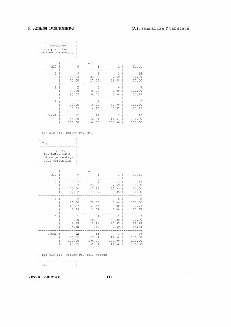
9. Analisi Quantitativa 9.1. summarize e tabulate
|-------------------|| frequency || row percentage || column percentage |+-------------------+
| a11a10 | 0 1 2 | Total
-----------+---------------------------------+----------0 | 9 3 1 | 13| 69.23 23.08 7.69 | 100.00| 75.00 27.27 33.33 | 50.00
-----------+---------------------------------+----------1 | 2 6 0 | 8| 25.00 75.00 0.00 | 100.00| 16.67 54.55 0.00 | 30.77
-----------+---------------------------------+----------2 | 1 2 2 | 5| 20.00 40.00 40.00 | 100.00| 8.33 18.18 66.67 | 19.23
-----------+---------------------------------+----------Total | 12 11 3 | 26
| 46.15 42.31 11.54 | 100.00| 100.00 100.00 100.00 | 100.00
. tab a10 a11, column row cell
+-------------------+| Key ||-------------------|| frequency || row percentage || column percentage || cell percentage |+-------------------+
| a11a10 | 0 1 2 | Total
-----------+---------------------------------+----------0 | 9 3 1 | 13| 69.23 23.08 7.69 | 100.00| 75.00 27.27 33.33 | 50.00| 34.62 11.54 3.85 | 50.00
-----------+---------------------------------+----------1 | 2 6 0 | 8| 25.00 75.00 0.00 | 100.00| 16.67 54.55 0.00 | 30.77| 7.69 23.08 0.00 | 30.77
-----------+---------------------------------+----------2 | 1 2 2 | 5| 20.00 40.00 40.00 | 100.00| 8.33 18.18 66.67 | 19.23| 3.85 7.69 7.69 | 19.23
-----------+---------------------------------+----------Total | 12 11 3 | 26
| 46.15 42.31 11.54 | 100.00| 100.00 100.00 100.00 | 100.00| 46.15 42.31 11.54 | 100.00
. tab a10 a11, column row cell nofreq
+-------------------+| Key |
Nicola Tommasi 101

9.1. summarize e tabulate 9. Analisi Quantitativa
|-------------------|| row percentage || column percentage || cell percentage |+-------------------+
| a11a10 | 0 1 2 | Total
-----------+---------------------------------+----------0 | 69.23 23.08 7.69 | 100.00| 75.00 27.27 33.33 | 50.00| 34.62 11.54 3.85 | 50.00
-----------+---------------------------------+----------1 | 25.00 75.00 0.00 | 100.00| 16.67 54.55 0.00 | 30.77| 7.69 23.08 0.00 | 30.77
-----------+---------------------------------+----------2 | 20.00 40.00 40.00 | 100.00| 8.33 18.18 66.67 | 19.23| 3.85 7.69 7.69 | 19.23
-----------+---------------------------------+----------Total | 46.15 42.31 11.54 | 100.00
| 100.00 100.00 100.00 | 100.00| 46.15 42.31 11.54 | 100.00
. tab a10 a11, chi2
| a11a10 | 0 1 2 | Total
-----------+---------------------------------+----------0 | 9 3 1 | 131 | 2 6 0 | 82 | 1 2 2 | 5
-----------+---------------------------------+----------Total | 12 11 3 | 26
Pearson chi2(4) = 10.7803 Pr = 0.029
. tab a10 a11, sum(pain)
Means, Standard Deviations and Frequencies of pain
| a11a10 | 0 1 2 | Total
-----------+---------------------------------+----------0 | 91.975309 87.962962 77.777779 | 89.957265| 5.4582514 12.525694 0 | 7.9006867| 9 3 1 | 13
-----------+---------------------------------+----------1 | 93.055557 65.74074 . | 72.569444| 9.8209251 15.180667 . | 18.392012| 2 6 0 | 8
-----------+---------------------------------+----------2 | 77.777779 40.277777 50 | 51.666666| 0 5.8925556 3.9283722 | 15.78697| 1 2 2 | 5
-----------+---------------------------------+----------Total | 90.972223 67.171716 59.25926 | 77.24359
| 6.9191447 20.631174 16.276293 | 19.657864| 12 11 3 | 26
Di nuovo, se vogliamo incrociare a coppie più di 2 variabili il comando da usareè:
102 Nicola Tommasi

9. Analisi Quantitativa 9.1. summarize e tabulate
tab2 varlist[if
][in
][weight
][, options
]che restituisce le distribuzioni di frequenza per ciascuna coppia delle variabilispecificate in varlist.
. tab2 s1 s2 s3 s4
-> tabulation of s1 by s2
| s2s1 | 0 1 2 3 4 | Total
-----------+-------------------------------------------------------+----------0 | 2 8 1 2 3 | 161 | 1 1 2 1 0 | 52 | 0 0 3 0 0 | 33 | 0 0 1 0 0 | 14 | 1 0 0 0 0 | 1
-----------+-------------------------------------------------------+----------Total | 4 9 7 3 3 | 26
-> tabulation of s1 by s3
| s3s1 | 0 1 2 | Total
-----------+---------------------------------+----------0 | 16 0 0 | 161 | 3 1 1 | 52 | 1 1 1 | 33 | 1 0 0 | 14 | 1 0 0 | 1
-----------+---------------------------------+----------Total | 22 2 2 | 26
-> tabulation of s1 by s4
| s4s1 | 0 1 4 | Total
-----------+---------------------------------+----------0 | 13 0 3 | 161 | 3 0 2 | 52 | 1 1 1 | 33 | 1 0 0 | 14 | 1 0 0 | 1
-----------+---------------------------------+----------Total | 19 1 6 | 26
-> tabulation of s2 by s3
| s3s2 | 0 1 2 | Total
-----------+---------------------------------+----------0 | 3 1 0 | 41 | 9 0 0 | 92 | 4 1 2 | 73 | 3 0 0 | 34 | 3 0 0 | 3
-----------+---------------------------------+----------Total | 22 2 2 | 26
-> tabulation of s2 by s4
Nicola Tommasi 103

9.1. summarize e tabulate 9. Analisi Quantitativa
| s4s2 | 0 1 4 | Total
-----------+---------------------------------+----------0 | 2 0 2 | 41 | 8 0 1 | 92 | 5 1 1 | 73 | 2 0 1 | 34 | 2 0 1 | 3
-----------+---------------------------------+----------Total | 19 1 6 | 26
-> tabulation of s3 by s4
| s4s3 | 0 1 4 | Total
-----------+---------------------------------+----------0 | 18 0 4 | 221 | 0 0 2 | 22 | 1 1 0 | 2
-----------+---------------------------------+----------Total | 19 1 6 | 26
9.1.1 Qualcosa di più avanzato
Per produrre tabelle di statistiche più evolute possiamo ricorre al comandotable
table rowvar[colvar
[supercolvar
] ] [if
][in
][weight
][, options
]dove in rowvar
[colvar
[supercolvar
] ]inseriamo variabili categoriche (fino ad
un massimo di 3).Tra le options inseriamo contents(clist) dove clist può essere scelto tra
mean varname media di varnamesd varname deviazione standard di varnamesum varname sommatoria di varnamen varname numero di casi (missing esclusi) di varnamemax varname valore massimo di varnamemin varname valore minimo di varnamemedian varname mediana di varnamep1 varname 1° percentile di varnamep2 varname 2° percentile di varname......p98 varname 98° percentile di varnamep99 varname 98° percentile di varnameiqr varname range interquartile (p75-p25) di varname
si tenga presente che al massimo si possono inserire 5 statistiche in clist.
. table fsize, c(mean w_food mean w_cloth mean w_house
104 Nicola Tommasi

9. Analisi Quantitativa 9.1. summarize e tabulate
mean w_trasporti mean w_eduricr) format(%5.3f) row col;
--------------------------------------------------------------------------------Numero di |component |i | mean(w_food) mean(w_cl~h) mean(w_ho~e) mean(w_tr~i) mean(w_ed~r)----------+---------------------------------------------------------------------
2 | 0.328 0.137 0.154 0.243 0.1383 | 0.357 0.142 0.151 0.219 0.1304 | 0.373 0.139 0.139 0.217 0.1325 | 0.393 0.133 0.133 0.209 0.1326 | 0.416 0.123 0.129 0.198 0.1347 | 0.433 0.107 0.130 0.203 0.1288 | 0.527 0.072 0.091 0.171 0.1399 | 0.378 0.116 0.150 0.215 0.141|
Total | 0.366 0.139 0.144 0.220 0.132--------------------------------------------------------------------------------
. table fsize, c(mean w_food iqr w_food sd w_food n w_food) format(%5.3f) row col
------------------------------------------------------------------Numero di |component |i | mean(w_food) iqr(w_food) sd(w_food) N(w_food)----------+-------------------------------------------------------
2 | 0.328 0.159 0.117 1,1753 | 0.357 0.154 0.108 3,6034 | 0.373 0.145 0.105 4,6995 | 0.393 0.149 0.107 1,1156 | 0.416 0.137 0.103 1627 | 0.433 0.132 0.109 268 | 0.527 0.111 0.078 29 | 0.378 0.248 0.176 2|
Total | 0.366 0.151 0.109 10,784------------------------------------------------------------------
. table fsize nch05, c(mean w_food mean w_cloth mean w_house meanw_trasporti mean w_eduricr) format(%5.3f) row col;
---------------------------------------------Numero di |component | Figli del capofamiglia <=5i | 0 1 2 3 Total----------+----------------------------------
2 | 0.328 0.328| 0.137 0.137| 0.154 0.154| 0.243 0.243| 0.138 0.138|
3 | 0.363 0.344 0.357| 0.131 0.166 0.142| 0.152 0.149 0.151| 0.224 0.210 0.219| 0.129 0.131 0.130|
4 | 0.373 0.377 0.365 0.373| 0.134 0.152 0.162 0.139| 0.138 0.140 0.142 0.139| 0.224 0.196 0.198 0.217| 0.132 0.135 0.133 0.132|
5 | 0.392 0.397 0.394 0.357 0.393
Nicola Tommasi 105

9.1. summarize e tabulate 9. Analisi Quantitativa
| 0.130 0.139 0.152 0.184 0.133| 0.134 0.135 0.116 0.155 0.133| 0.215 0.191 0.197 0.136 0.209| 0.129 0.139 0.141 0.168 0.132|
6 | 0.415 0.406 0.460 0.416| 0.122 0.125 0.124 0.123| 0.125 0.142 0.119 0.129| 0.205 0.187 0.168 0.198| 0.132 0.140 0.130 0.134|
7 | 0.415 0.439 0.459 0.522 0.433| 0.105 0.108 0.106 0.122 0.107| 0.119 0.126 0.161 0.173 0.130| 0.240 0.186 0.146 0.022 0.203| 0.120 0.140 0.128 0.161 0.128|
8 | 0.582 0.471 0.527| 0.083 0.061 0.072| 0.075 0.107 0.091| 0.161 0.181 0.171| 0.099 0.180 0.139|
9 | 0.254 0.502 0.378| 0.117 0.115 0.116| 0.181 0.119 0.150| 0.313 0.117 0.215| 0.135 0.147 0.141|
Total | 0.366 0.363 0.372 0.371 0.366| 0.133 0.157 0.159 0.178 0.139| 0.144 0.144 0.138 0.157 0.144| 0.225 0.202 0.197 0.126 0.220| 0.131 0.133 0.134 0.168 0.132
---------------------------------------------
Se invece abbiamo variabili continue di cui vogliamo avere ulteriori statisticheoltre a quelle fornite da summarize possiamo ricorrere a:
tabstat varlist[if
][in
][weight
][, options
]dove in varlist inseriamo la liste delle variabili continue e tra le options instatistics() possiamo scegliere tra:
meannsummaxminsdvariancecv coefficiente di variazione (sd/mean)semean errore standard della media (sd/sqrt(n))skewness (indice di simmetria o indice di Pearson)kurtosis (indice di curtosi o di appiattimento)p1p5
106 Nicola Tommasi

9. Analisi Quantitativa 9.1. summarize e tabulate
p10p25medianp50p75p90p95p99range = max - miniqr = p75 - p25q equivalente a p25 p50 p75
. tabstat tax_1-tax_8 if nfigli==1,by(prof_nmr) stats(sum mean cv p1 p99) col(stat) long notot;
prof_nmr variable | sum mean cv p1 p99----------------------+--------------------------------------------------6 tax_1 | 81598.11 799.9815 1.965136 0 5761.707
tax_2 | -18165.78 -178.0959 -1.018802 -565.1445 0tax_3 | 0 0 . 0 0tax_4 | 0 0 . 0 0tax_5 | 31253.79 306.4097 1.099732 0 1039.958tax_6 | 54422.84 533.5573 1.099732 0 1810.899tax_7 | 812.8596 7.969212 1.099732 0 27.04759tax_8 | 1013.78 9.939017 1.099732 0 33.73313
----------------------+--------------------------------------------------7 tax_1 | 221761.5 2174.132 1.409285 0 8196.94
tax_2 | -21492.1 -210.7069 -1.001891 -568.2259 0tax_3 | -4326.881 -42.4204 -1.678715 -220.315 0tax_4 | 0 0 . 0 0tax_5 | 36993.11 362.6776 1.034861 0 1113.488tax_6 | 64416.83 631.5376 1.034861 0 1938.939tax_7 | 962.1299 9.432646 1.034861 0 28.96tax_8 | 1199.946 11.76418 1.034861 0 36.11824
----------------------+--------------------------------------------------8 tax_1 | 383905.5 3763.779 1.378702 0 13930.61
tax_2 | -1766 -17.31372 -1.068916 -58.87674 0tax_3 | -4017.233 -39.38464 -1.64311 -201.7244 0tax_4 | 0 0 . 0 0tax_5 | 52293.15 512.6779 1.008443 0 1556.057tax_6 | 91059.09 892.7361 1.008443 0 2709.592tax_7 | 1360.059 13.33391 1.008443 0 40.47047tax_8 | 1696.234 16.62974 1.008443 0 50.47383
----------------------+--------------------------------------------------9 tax_1 | 335143.8 3285.724 1.336498 0 12298.62
tax_2 | -1770.913 -17.36189 -1.160488 -68.73045 0tax_3 | -4191.114 -41.08936 -1.643618 -194.5484 0tax_4 | 0 0 . 0 0tax_5 | 50404.86 494.1653 1.049721 0 1543.804tax_6 | 87770.97 860.4997 1.049721 0 2688.256tax_7 | 1310.947 12.85242 1.049721 0 40.15179tax_8 | 1634.983 16.02925 1.049721 0 50.07639
----------------------+--------------------------------------------------10 tax_1 | 221761.5 2174.132 1.409285 0 8196.94
tax_2 | -21492.1 -210.7069 -1.001891 -568.2259 0tax_3 | -4326.881 -42.4204 -1.678715 -220.315 0tax_4 | 0 0 . 0 0tax_5 | 36993.11 362.6776 1.034861 0 1113.488tax_6 | 64416.83 631.5376 1.034861 0 1938.939
Nicola Tommasi 107
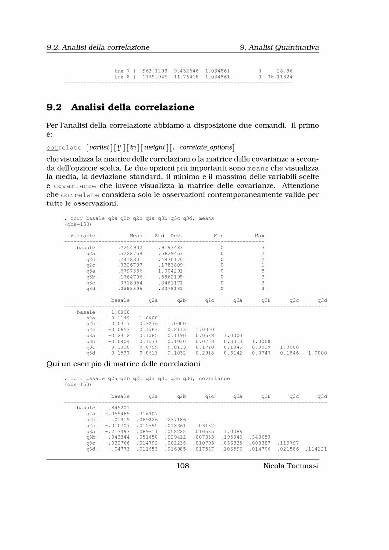
9.2. Analisi della correlazione 9. Analisi Quantitativa
tax_7 | 962.1299 9.432646 1.034861 0 28.96tax_8 | 1199.946 11.76418 1.034861 0 36.11824
-------------------------------------------------------------------------
9.2 Analisi della correlazione
Per l’analisi della correlazione abbiamo a disposizione due comandi. Il primoè:
correlate[varlist
][if
][in
][weight
][, correlate_options
]che visualizza la matrice delle correlazioni o la matrice delle covarianze a secon-da dell’opzione scelta. Le due opzioni più importanti sono means che visualizzala media, la deviazione standard, il minimo e il massimo delle variabili sceltee covariance che invece visualizza la matrice delle covarianze. Attenzioneche correlate considera solo le osservazioni contemporaneamente valide pertutte le osservazioni.
. corr basale q2a q2b q2c q3a q3b q3c q3d, means(obs=153)
Variable | Mean Std. Dev. Min Max-----------+----------------------------------------------------
basale | .7254902 .9193483 0 3q2a | .5228758 .5629453 0 2q2b | .2418301 .4870176 0 2q2c | .0326797 .1783809 0 1q3a | .6797386 1.004291 0 5q3b | .1764706 .5862195 0 3q3c | .0718954 .3461171 0 3q3d | .0653595 .3378181 0 3
| basale q2a q2b q2c q3a q3b q3c q3d-----------+------------------------------------------------------------------------
basale | 1.0000q2a | -0.1149 1.0000q2b | 0.0317 0.3276 1.0000q2c | -0.0653 0.1563 0.2113 1.0000q3a | -0.2312 0.1585 0.1190 0.0588 1.0000q3b | -0.0804 0.1571 0.1030 0.0703 0.3313 1.0000q3c | -0.1030 0.0759 0.0133 0.1748 0.1045 0.0019 1.0000q3d | -0.1537 0.0613 0.1032 0.2918 0.3142 0.0743 0.1846 1.0000
Qui un esempio di matrice delle correlazioni
. corr basale q2a q2b q2c q3a q3b q3c q3d, covariance(obs=153)
| basale q2a q2b q2c q3a q3b q3c q3d-----------+------------------------------------------------------------------------
basale | .845201q2a | -.059469 .316907q2b | .01419 .089826 .237186q2c | -.010707 .015695 .018361 .03182q3a | -.213493 .089611 .058222 .010535 1.0086q3b | -.043344 .051858 .029412 .007353 .195046 .343653q3c | -.032766 .014792 .002236 .010793 .036335 .000387 .119797q3d | -.04773 .011653 .016985 .017587 .106596 .014706 .021586 .114121
108 Nicola Tommasi

9. Analisi Quantitativa 9.3. Analisi outliers
Il secondo comando è:
pwcorr[varlist
][if
][in
][weight
][, pwcorr_options
]che analizza le correlazioni indipendentemente per ciascuna coppia di vari-abili, per cui la numerosità fa’ riferimento al numero di osservazioni valido perciascuna coppia di variabili. Le opzioni principali sono:
obs visualizza il numero di osservazioni per ciascuna coppia di variabilisig visualizza il livello di significatività della correlazionestar(#) visualizza con * i livelli di significatività inferiori al valore #bonferroni usa il metodo di Bonferroni per correggere il livello di significativ-
itàsidak usa il metodo di Sidak per correggere il livello di significatività
. pwcorr basale q2a q2b q2c q3a q3b q3c q3d, star(0.05) obs sig
| valsalva q2a q2b q2c q3a q3b q3c q3d-----------+------------------------------------------------------------------------
valsalva | 1.0000|| 153|
q2a | 0.0507 1.0000| 0.5338| 153 162|
q2b | 0.0218 0.3270* 1.0000| 0.7895 0.0000| 153 162 162|
q2c | 0.0246 0.1559* 0.2148* 1.0000| 0.7631 0.0476 0.0061| 153 162 162 162|
q3a | -0.1235 0.1642* 0.1228 0.0602 1.0000| 0.1283 0.0368 0.1195 0.4464| 153 162 162 162 162|
q3b | 0.0031 0.1102 0.0830 0.0606 0.3190* 1.0000| 0.9694 0.1628 0.2939 0.4433 0.0000| 153 162 162 162 162 162|
q3c | -0.1163 0.0779 0.0189 0.1766* 0.1055 -0.0031 1.0000| 0.1522 0.3245 0.8115 0.0246 0.1814 0.9683| 153 162 162 162 162 162 162|
q3d | -0.1587 0.0634 0.1078 0.2932* 0.3117* 0.0640 0.1864* 1.0000| 0.0501 0.4232 0.1723 0.0002 0.0001 0.4182 0.0175| 153 162 162 162 162 162 162 162|
9.3 Analisi outliers
Tralasciando tutta la teoria attinente al problema dei dati anomali (o outliers),vediamo come Stata ci permette di identificarli. Il comando ufficiale è:
Nicola Tommasi 109

9.3. Analisi outliers 9. Analisi Quantitativa
hadimvo varlist[if
][in
], generate(newvar1
[newvar2
])
[p(#)
]dove la nuova variabile generata newvar1 (o le nuove variabili generate nelcaso di analisi multivariata) sono delle dummy che identificato con 1 i valoricandidati ad essere outliers.Il secondo comando, che va aggiunto tramite ssc, è:
grubbs varlist[if
][in
][, options
]dove tra le opzioni teniamo presenti:
drop che elimina le osservazioni identificate come outliersgenerate(newvar1 ...) che crea variabili dummy per identificare i valori
outlierslog che il log delle iterazioni
Come sempre segue l’esempio di utilizzo dei due comandi. Notate la differen-za nei tempi di esecuzione tra i due comandi e il fatto che restituiscono ilmedesimo risultato.
. local st = "$S_TIME";
. hadimvo isee, gen(flag_isee);
Beginning number of observations: 13239Initially accepted: 2Expand to (n+k+1)/2: 6620
Expand, p = .05: 13226Outliers remaining: 13
. elapse `st´;Elapsed time was 24 minutes, 33 seconds.
. list id isee if flag_isee==1, sep(0);
+-------------------+| id isee ||-------------------|
13227. | 6874 63867.1 |13228. | 6875 64486.92 |13229. | 6876 67414.06 |13230. | 6877 72366.19 |13231. | 13234 73208.93 |13232. | 13235 73449.813 |13233. | 13236 77971.492 |13234. | 13237 78410.148 |13235. | 13238 84195.203 |13236. | 13239 88253.977 |13237. | 6878 93771.63 |13238. | 6880 127160.35 |13239. | 6879 127160.35 |
+-------------------+
. drop flag_isee;
. local st = "$S_TIME";
. grubbs isee, gen(flag_isee) log;Variable: isee (0/1 variable recording which observations are outliers: flag_isee).Iteration = 1. T-value: 10.7325 so 127160.35 is an outlier
110 Nicola Tommasi
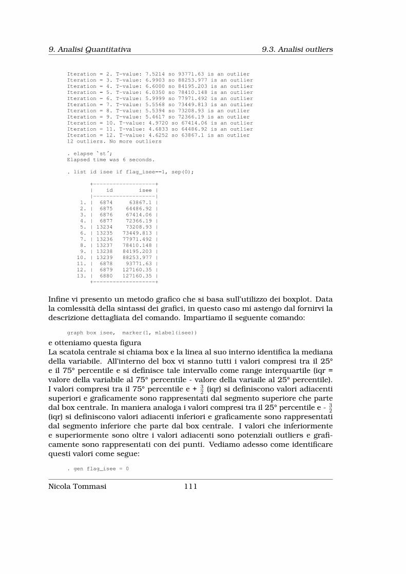
9. Analisi Quantitativa 9.3. Analisi outliers
Iteration = 2. T-value: 7.5214 so 93771.63 is an outlierIteration = 3. T-value: 6.9903 so 88253.977 is an outlierIteration = 4. T-value: 6.6000 so 84195.203 is an outlierIteration = 5. T-value: 6.0350 so 78410.148 is an outlierIteration = 6. T-value: 5.9999 so 77971.492 is an outlierIteration = 7. T-value: 5.5568 so 73449.813 is an outlierIteration = 8. T-value: 5.5394 so 73208.93 is an outlierIteration = 9. T-value: 5.4617 so 72366.19 is an outlierIteration = 10. T-value: 4.9720 so 67414.06 is an outlierIteration = 11. T-value: 4.6833 so 64486.92 is an outlierIteration = 12. T-value: 4.6252 so 63867.1 is an outlier12 outliers. No more outliers
. elapse `st´;Elapsed time was 6 seconds.
. list id isee if flag_isee==1, sep(0);
+-------------------+| id isee ||-------------------|
1. | 6874 63867.1 |2. | 6875 64486.92 |3. | 6876 67414.06 |4. | 6877 72366.19 |5. | 13234 73208.93 |6. | 13235 73449.813 |7. | 13236 77971.492 |8. | 13237 78410.148 |9. | 13238 84195.203 |10. | 13239 88253.977 |11. | 6878 93771.63 |12. | 6879 127160.35 |13. | 6880 127160.35 |
+-------------------+
Infine vi presento un metodo grafico che si basa sull’utilizzo dei boxplot. Datala comlessità della sintassi dei grafici, in questo caso mi astengo dal fornirvi ladescrizione dettagliata del comando. Impartiamo il seguente comando:
graph box isee, marker(1, mlabel(isee))
e otteniamo questa figuraLa scatola centrale si chiama box e la linea al suo interno identifica la medianadella variabile. All’interno del box vi stanno tutti i valori compresi tra il 25°e il 75° percentile e si definisce tale intervallo come range interquartile (iqr =valore della variabile al 75° percentile - valore della variaile al 25° percentile).I valori compresi tra il 75° percentile e + 3
2 (iqr) si definiscono valori adiacentisuperiori e graficamente sono rappresentati dal segmento superiore che partedal box centrale. In maniera analoga i valori compresi tra il 25° percentile e - 3
2(iqr) si definiscono valori adiacenti inferiori e graficamente sono rappresentatidal segmento inferiore che parte dal box centrale. I valori che inferiormentee superiormente sono oltre i valori adiacenti sono potenziali outliers e grafi-camente sono rappresentati con dei punti. Vediamo adesso come identificarequesti valori come segue:
. gen flag_isee = 0
Nicola Tommasi 111

9.3. Analisi outliers 9. Analisi Quantitativa
Figura 9.1: Box Plot
112 Nicola Tommasi
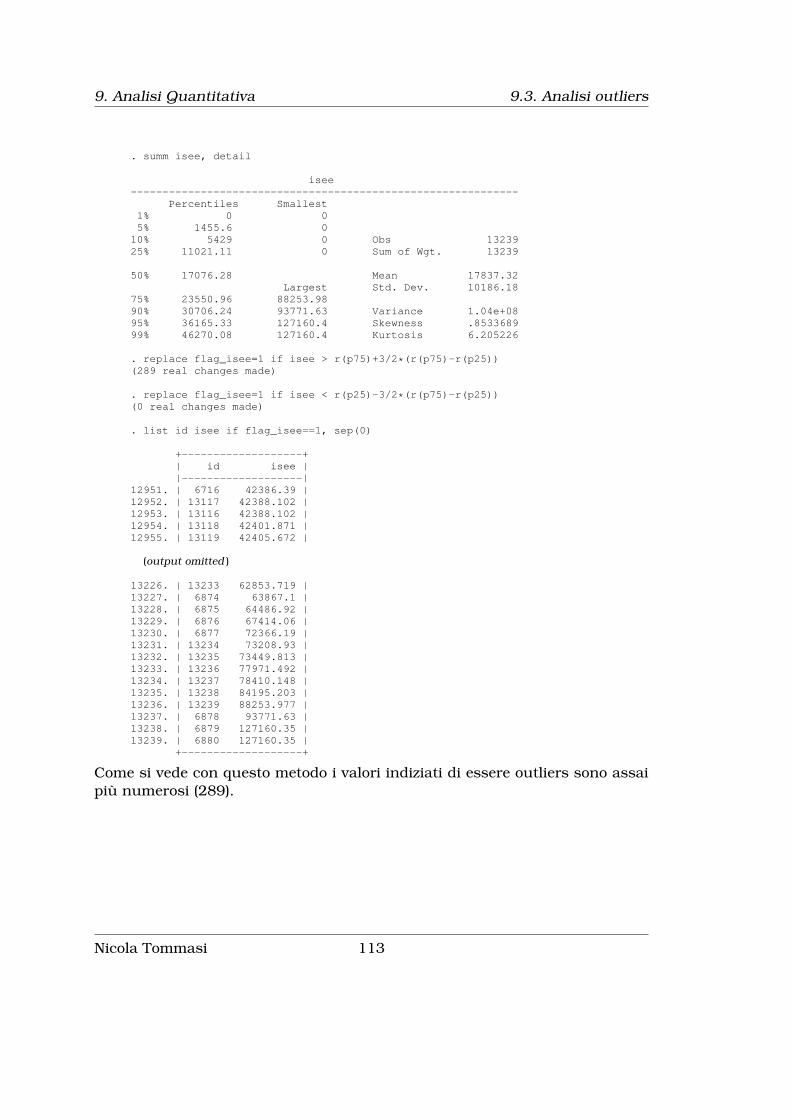
9. Analisi Quantitativa 9.3. Analisi outliers
. summ isee, detail
isee-------------------------------------------------------------
Percentiles Smallest1% 0 05% 1455.6 010% 5429 0 Obs 1323925% 11021.11 0 Sum of Wgt. 13239
50% 17076.28 Mean 17837.32Largest Std. Dev. 10186.18
75% 23550.96 88253.9890% 30706.24 93771.63 Variance 1.04e+0895% 36165.33 127160.4 Skewness .853368999% 46270.08 127160.4 Kurtosis 6.205226
. replace flag_isee=1 if isee > r(p75)+3/2*(r(p75)-r(p25))(289 real changes made)
. replace flag_isee=1 if isee < r(p25)-3/2*(r(p75)-r(p25))(0 real changes made)
. list id isee if flag_isee==1, sep(0)
+-------------------+| id isee ||-------------------|
12951. | 6716 42386.39 |12952. | 13117 42388.102 |12953. | 13116 42388.102 |12954. | 13118 42401.871 |12955. | 13119 42405.672 |
(output omitted )
13226. | 13233 62853.719 |13227. | 6874 63867.1 |13228. | 6875 64486.92 |13229. | 6876 67414.06 |13230. | 6877 72366.19 |13231. | 13234 73208.93 |13232. | 13235 73449.813 |13233. | 13236 77971.492 |13234. | 13237 78410.148 |13235. | 13238 84195.203 |13236. | 13239 88253.977 |13237. | 6878 93771.63 |13238. | 6879 127160.35 |13239. | 6880 127160.35 |
+-------------------+
Come si vede con questo metodo i valori indiziati di essere outliers sono assaipiù numerosi (289).
Nicola Tommasi 113


Capitolo 10
Trasformare Dataset
10.1 Aggiungere osservazioni
In genere quando si aggiungono osservazioni provenienti da un altro datasetsi richiede che le variabili abbiano lo stesso nome, mentre non è richiesto chesiano nello stesso ordine di posizione; vedi secondo dove la disposizione dellevariabili è c, b, a. Graficamente ciò che vogliamo ottenere è:
+-------------+| master ||-------------| +----------------+| a b c | | risultato || | |----------------|| 1 2 3 | | a b c || 4 5 6 | | |+-------------+ | 1 2 3 |
+ ------->> | 4 5 6 |+-------------+ | 7 8 9 || secondo | | 10 11 12 ||-------------| | 13 14 15 || c b a | +----------------+| || 9 8 7 || 12 11 10 || 15 14 13 |+-------------+
Il primo passo è caricare il primo dataset, poi si aggiungono le osservazioni delsecondo dataset tramite il comando:
append using filename[, options
]115

10.2. Aggiungere variabili 10. Trasformare Dataset
dove in filename specifichiamo il dataset da aggiungere e dove tra le options c’èkeep(varlist) dove è possibile specificare le variabili da prendere nel datasetche viene aggiunto.
Si tenga presente che se una variabile è presente in uno solo dei due dataset,nel dataset unione (risultato) per quella variabile ci saranno delle osser-vazioni missing in corrispondenza delle osservazioni del dataset in cui non erapresente.
+-------------+| secondo ||-------------|| a b c | +------------------+| | | risultato || 7 8 9 | |------------------|| 10 11 12 | | a b c d || 13 14 15 | | |+-------------+ | 7 8 9 . |
+ ------>> | 10 11 12 . |+--------------+ | 13 14 15 . || master | | 1 2 3 7 ||--------------+ | 4 5 6 8 || a b c d | +------------------+| || 1 2 3 7 || 4 5 6 8 |+--------------+
In conclusione il comando append serve essenzialmente per aggiungere osser-vazioni, e solo indirettamente per aggiungere variabili.
10.2 Aggiungere variabili
Condizione necessaria per aggiungere ad un dataset (master) variabili prove-nienti da un altro dataset (slave) è che in entrambi siano presenti una o piùvariabili che permettano di stabilire una relazione biunivoca tra le osservazionidel primo e del secondo dataset. In altre parole ci devono essere delle vari-abili chiave che mi permettano di assegnare ciascun valore Xij proveniente daldataset slave ad una determinata osservazione del dataset master.In Stata il comando che permettere di compiere questa operazione è merge .Nelle versioni precedenti di Stata tale comando prevedeva che i dataset mastere slave fossero già ordinati in base alle variabili chiave per cui non era moltoagevole da usare. Qui si farà ricorso al comando mmerge, che permette disuperare questa limitazione e che in più ha delle opzioni assai utili.
116 Nicola Tommasi
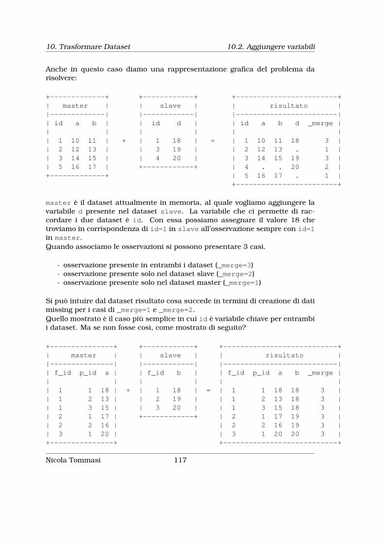
10. Trasformare Dataset 10.2. Aggiungere variabili
Anche in questo caso diamo una rappresentazione grafica del problema darisolvere:
+-------------+ +------------+ +------------------------+| master | | slave | | risultato ||-------------| |------------| |------------------------|| id a b | | id d | | id a b d _merge || | | | | || 1 10 11 | + | 1 18 | = | 1 10 11 18 3 || 2 12 13 | | 3 19 | | 2 12 13 . 1 || 3 14 15 | | 4 20 | | 3 14 15 19 3 || 5 16 17 | +------------+ | 4 . . 20 2 |+-------------+ | 5 16 17 . 1 |
+------------------------+
master è il dataset attualmente in memoria, al quale vogliamo aggiungere lavariabile d presente nel dataset slave. La variabile che ci permette di rac-cordare i due dataset è id. Con essa possiamo assegnare il valore 18 chetroviamo in corrispondenza di id=1 in slave all’osservazione sempre con id=1in master.Quando associamo le osservazioni si possono presentare 3 casi.
- osservazione presente in entrambi i dataset (_merge=3)- osservazione presente solo nel dataset slave (_merge=2)- osservazione presente solo nel dataset master (_merge=1)
Si può intuire dal dataset risultato cosa succede in termini di creazione di datimissing per i casi di _merge=1 e _merge=2.Quello mostrato è il caso più semplice in cui id è variabile chiave per entrambii dataset. Ma se non fosse così, come mostrato di seguito?
+---------------+ +------------+ +---------------------------+| master | | slave | | risultato ||---------------| |------------| |---------------------------|| f_id p_id a | | f_id b | | f_id p_id a b _merge || | | | | || 1 1 18 | + | 1 18 | = | 1 1 18 18 3 || 1 2 13 | | 2 19 | | 1 2 13 18 3 || 1 3 15 | | 3 20 | | 1 3 15 18 3 || 2 1 17 | +------------+ | 2 1 17 19 3 || 2 2 16 | | 2 2 16 19 3 || 3 1 20 | | 3 1 20 20 3 |+---------------+ +---------------------------+
Nicola Tommasi 117

10.2. Aggiungere variabili 10. Trasformare Dataset
In questo caso l’informazione contenuta in b si “spalma” su tutti i p_id chehanno lo stesso f_id di master. Consiglio, per comodità, di usare semprecome master il dataset che ha il numero maggiore di variabili chiave.
Come accennato in precedenza il comando mmerge non prevede che i duedataset siano preventivamente ordinati; questa è la sua sintassi:
mmerge match-variable(s) using filename[, options
]dove in match-variable(s) vanno indicate la/le variabile/i che servono da rac-cordo tra i due dataset, in filename il percorso e il nome del dataset che fungeda slave. Tra le principali options citiamo:
ukeep(varlist) dove in varlist vengono indicate le variabili che vogliamo ag-giungere dal dataset filename. Se non viene indicato nulla, verrannoaggiunte tutte le variabili di filename.
udrop(varlist) dove in varlist vengono indicate le variabili che non vogliamoaggiungere dal dataset filename.
update Piccola spiegazione. Di default il dataset master è inviolabile ossianel dataset risultante dal merge saranno tenuti i valori delle variabili deldataset master anche se queste stesse sono presenti nello slave ed han-no valori diversi. Se viene specificata questa opzione verrà preso il valoredel dataset using nel caso in cui nel master vi siano valori missing.
replace deve essere specificata anche l’opzione update. Con questa opzionei valori non missing del master saranno sostituiti con i corrispondentivalori non missing dello slave quando non corrispondenti. Comunqueun valore non missing del master non verrà mai sostituito con un valoremissing dello slave.
uname(stub) specifica il prefisso da aggiungere alle variabili importate daldataset slave.
Alcune di queste opzioni sono un po’ complicate quindi vediamo alcuni esempi.
. use master,clear
. clist
mat corso fac1. VR0001 M50 M2. VR0002 E3. VR0003 S07 S4. VR0004 L12 L5. VR0005 L08 L6. VR0006 S33 S7. VR0007 E07 E8. VR0008 G02 G
. use SLAVE, clear
. clist
mat corso fac disab partime
118 Nicola Tommasi

10. Trasformare Dataset 10.2. Aggiungere variabili
1. VR0001 M50 M 1 PT2. VR0002 E01 E 03. VR0003 . S 04. VR0004 L12 L 0 PT5. VR0005 L08 L 06. VR0006 S33 S 17. VR0007 E07 E 08. VR0008 G08 G 0 PT
Opzione ukeep(varlist)
. use MASTER, clear
. mmerge mat using SLAVE, ukeep(disab)
-------------------------------------------------------------------------------merge specs |
matching type | automv´s on match vars | noneunmatched obs from | both
---------------------+---------------------------------------------------------master file | MASTER.dta
obs | 8vars | 3
match vars | mat (key)-------------------+---------------------------------------------------------using file | SLAVE.dta
obs | 8vars | 2 (selection via udrop/ukeep)
match vars | mat (key)---------------------+---------------------------------------------------------result file | MASTER.dta
obs | 8vars | 6 (including _merge)
------------+---------------------------------------------------------_merge | 8 obs both in master and using data (code==3)
-------------------------------------------------------------------------------
. clist
mat corso fac disab _merge1. VR0001 M50 M 1 both in master and using data2. VR0002 E 0 both in master and using data3. VR0003 S07 S 0 both in master and using data4. VR0004 L12 L 0 both in master and using data5. VR0005 L08 L 0 both in master and using data6. VR0006 S33 S 1 both in master and using data7. VR0007 E07 E 0 both in master and using data8. VR0008 G02 G 0 both in master and using data
Opzione udrop(varlist)
. use MASTER, clear
. mmerge mat using SLAVE, udrop(disab)
-------------------------------------------------------------------------------merge specs |
matching type | automv´s on match vars | noneunmatched obs from | both
---------------------+---------------------------------------------------------master file | MASTER.dta
obs | 8
Nicola Tommasi 119

10.2. Aggiungere variabili 10. Trasformare Dataset
vars | 3match vars | mat (key)
-------------------+---------------------------------------------------------using file | SLAVE.dta
obs | 8vars | 4 (selection via udrop/ukeep)
match vars | mat (key)-------------------+---------------------------------------------------------
common vars | corso fac---------------------+---------------------------------------------------------result file | MASTER.dta
obs | 8vars | 6 (including _merge)
------------+---------------------------------------------------------_merge | 8 obs both in master and using data (code==3)
-------------------------------------------------------------------------------
. clist
mat corso fac partime _merge1. VR0001 M50 M PT both in master and using data2. VR0002 E both in master and using data3. VR0003 S07 S both in master and using data4. VR0004 L12 L PT both in master and using data5. VR0005 L08 L both in master and using data6. VR0006 S33 S both in master and using data7. VR0007 E07 E both in master and using data8. VR0008 G02 G PT both in master and using data
Opzione update (Prestate attenzione a cosa succede alla variabile corso)
. use MASTER, clear
. mmerge mat using SLAVE
-------------------------------------------------------------------------------merge specs |
matching type | automv´s on match vars | noneunmatched obs from | both
---------------------+---------------------------------------------------------master file | MASTER.dta
obs | 8vars | 3
match vars | mat (key)-------------------+---------------------------------------------------------using file | SLAVE.dta
obs | 8vars | 5
match vars | mat (key)-------------------+---------------------------------------------------------
common vars | corso fac---------------------+---------------------------------------------------------result file | MASTER.dta
obs | 8vars | 7 (including _merge)
------------+---------------------------------------------------------_merge | 8 obs both in master and using data (code==3)
-------------------------------------------------------------------------------
. drop _merge
. clist
mat corso fac disab partime
120 Nicola Tommasi

10. Trasformare Dataset 10.2. Aggiungere variabili
1. VR0001 M50 M 1 PT2. VR0002 E 03. VR0003 S07 S 04. VR0004 L12 L 0 PT5. VR0005 L08 L 06. VR0006 S33 S 17. VR0007 E07 E 08. VR0008 G02 G 0 PT
. use MASTER, clear
. mmerge mat using SLAVE, update
-------------------------------------------------------------------------------merge specs |
matching type | automv´s on match vars | noneunmatched obs from | both
---------------------+---------------------------------------------------------master file | MASTER.dta
obs | 8vars | 3
match vars | mat (key)-------------------+---------------------------------------------------------using file | SLAVE.dta
obs | 8vars | 5
match vars | mat (key)-------------------+---------------------------------------------------------
common vars | corso fac---------------------+---------------------------------------------------------result file | MASTER.dta
obs | 8vars | 7 (including _merge)
------------+---------------------------------------------------------_merge | 5 obs in both, master agrees with using data (code==3)
| 1 obs in both, missing in master data updated (code==4)| 2 obs in both, master disagrees with using data (code==5)
-------------------------------------------------------------------------------
. clist
mat corso fac disab partime _mergeVR0001 M50 M 1 PT in both, master agrees with using dataVR0002 E01 E 0 in both, missing in master data updatedVR0003 S07 S 0 in both, master disagrees with using dataVR0004 L12 L 0 PT in both, master agrees with using dataVR0005 L08 L 0 in both, master agrees with using dataVR0006 S33 S 1 in both, master agrees with using dataVR0007 E07 E 0 in both, master agrees with using dataVR0008 G02 G 0 PT in both, master disagrees with using data
Opzione replace
. use MASTER, clear
. mmerge mat using SLAVE, update replace
-------------------------------------------------------------------------------merge specs |
matching type | automv´s on match vars | noneunmatched obs from | both
---------------------+---------------------------------------------------------master file | MASTER.dta
Nicola Tommasi 121

10.2. Aggiungere variabili 10. Trasformare Dataset
obs | 8vars | 3
match vars | mat (key)-------------------+---------------------------------------------------------using file | SLAVE.dta
obs | 8vars | 5
match vars | mat (key)-------------------+---------------------------------------------------------
common vars | corso fac---------------------+---------------------------------------------------------result file | MASTER.dta
obs | 8vars | 7 (including _merge)
------------+---------------------------------------------------------_merge | 5 obs in both, master agrees with using data (code==3)
| 1 obs in both, missing in master data updated (code==4)| 2 obs in both, master disagrees with using data (code==5)
-------------------------------------------------------------------------------
. clist
mat corso fac disab partime _mergeVR0001 M50 M 1 PT in both, master agrees with using dataVR0002 E01 E 0 in both, missing in master data updatedVR0003 . S 0 in both, master disagrees with using dataVR0004 L12 L 0 PT in both, master agrees with using dataVR0005 L08 L 0 in both, master agrees with using dataVR0006 S33 S 1 in both, master agrees with using dataVR0007 E07 E 0 in both, master agrees with using dataVR0008 G08 G 0 PT in both, master disagrees with using data
Opzione uname(stub)
. use MASTER, clear
. mmerge mat using SLAVE, ukeep(corso fac disab) uname(chk_)
-------------------------------------------------------------------------------merge specs |
matching type | automv´s on match vars | noneunmatched obs from | both
---------------------+---------------------------------------------------------master file | MASTER.dta
obs | 8vars | 3
match vars | mat (key)-------------------+---------------------------------------------------------using file | SLAVE.dta
obs | 8vars | 4 (selection via udrop/ukeep)
match vars | mat (key)---------------------+---------------------------------------------------------result file | MASTER.dta
obs | 8vars | 8 (including _merge)
------------+---------------------------------------------------------_merge | 8 obs both in master and using data (code==3)
-------------------------------------------------------------------------------
. drop _merge
. clist
122 Nicola Tommasi

10. Trasformare Dataset 10.3. Collassare un dataset
mat corso fac chk_corso chk_fac chk_di~b1. VR0001 M50 M M50 M 12. VR0002 E E01 E 03. VR0003 S07 S . S 04. VR0004 L12 L L12 L 05. VR0005 L08 L L08 L 06. VR0006 S33 S S33 S 17. VR0007 E07 E E07 E 08. VR0008 G02 G G08 G 0
In conclusione il comando mmerge serve essenzialmente per aggiungere vari-abili, e solo indirettamente per aggiungere osservazioni.
10.3 Collassare un dataset
Collassare un dataset vuol dire ridurre il numero delle sue osservazioni, trasfor-mando le informazioni contenute nelle righe che si vanno ad eliminare secon-do una certa funzione. È il caso per esempio di un dataset con informazionisugli individui che viene collassato in un dataset che contenga informazioniaggregate per singola famiglia di appartenenza. Il comando da usare è:
collapse clist[if
][in
][weight
][, options
]dove in clist si elencano le variabili che verranno collassate con la funzione daapplicare secondo lo schema(stat) varlisto(stat) new_var=varnameLe funzioni applicabili in stat sono:
- mean (opzione di default)- sd- sum- count- max- min- iqr- median- p1, p2,....p50, ..., p98, p99
Infine in by vanno le variabili che faranno da variabili chiave per il datasetcollassato.Se ne deduce che questo tipo di trattamento è applicabile solo a variabilinumeriche; le variabili che non vengono specificate in clist o in by verrannocancellate.
. list;
Nicola Tommasi 123

10.4. reshape di un dataset 10. Trasformare Dataset
+----------------------------+| gpa hour year number ||----------------------------|
1. | 3.2 30 1 3 |2. | 3.5 34 1 2 |3. | 2.8 28 1 9 |4. | 2.1 30 1 4 |5. | 3.8 29 2 3 |
|----------------------------|6. | 2.5 30 2 4 |7. | 2.9 35 2 5 |8. | 3.7 30 3 4 |9. | 2.2 35 3 2 |10. | 3.3 33 3 3 |
|----------------------------|11. | 3.4 32 4 5 |12. | 2.9 31 4 2 |
+----------------------------+
. collapse (count) n_gpa=gpa (mean) gpa (min) mingpa=gpa (max) maxgpa=gpa(mean) meangpa=gpa, by(year);
. list;
+------------------------------------------------------+| year n_gpa gpa mingpa maxgpa meangpa ||------------------------------------------------------|
1. | 1 4 2.9 2.1 3.5 2.9 |2. | 2 3 3.066667 2.5 3.8 3.066667 |3. | 3 3 3.066667 2.2 3.7 3.066667 |4. | 4 2 3.15 2.9 3.4 3.15 |
+------------------------------------------------------+
10.4 reshape di un dataset
Prima di spiegare il reshape, occorre introdurre il concetto di wide form e dilong form. Si considerino i seguenti esempi di dataset:
wide form: long form:
id sex inc80 inc81 id year sex inc----------------------- ----------------------1 0 5000 5500 1 80 0 50002 1 2000 2200 1 81 0 55003 0 3000 2000 2 80 1 2000
2 81 1 22003 80 0 30003 81 0 2000
I due dataset sono identici, contengono le stesse informazioni. Quello checambia è l’organizzazione delle informazioni. In Stata esiste un comando pertrasformare un dataset in wide form in un dataset in long form e viceversa.Innanzitutto si noti che il passaggio da un form all’altro comporta un cambi-
124 Nicola Tommasi
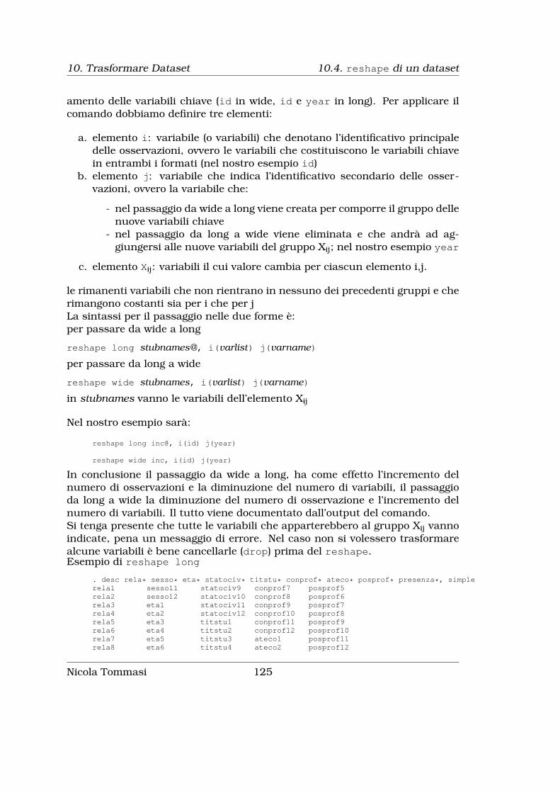
10. Trasformare Dataset 10.4. reshape di un dataset
amento delle variabili chiave (id in wide, id e year in long). Per applicare ilcomando dobbiamo definire tre elementi:
a. elemento i: variabile (o variabili) che denotano l’identificativo principaledelle osservazioni, ovvero le variabili che costituiscono le variabili chiavein entrambi i formati (nel nostro esempio id)
b. elemento j: variabile che indica l’identificativo secondario delle osser-vazioni, ovvero la variabile che:
- nel passaggio da wide a long viene creata per comporre il gruppo dellenuove variabili chiave
- nel passaggio da long a wide viene eliminata e che andrà ad ag-giungersi alle nuove variabili del gruppo Xij; nel nostro esempio year
c. elemento Xij: variabili il cui valore cambia per ciascun elemento i,j.
le rimanenti variabili che non rientrano in nessuno dei precedenti gruppi e cherimangono costanti sia per i che per jLa sintassi per il passaggio nelle due forme è:per passare da wide a long
reshape long stubnames@, i(varlist) j(varname)
per passare da long a wide
reshape wide stubnames, i(varlist) j(varname)
in stubnames vanno le variabili dell’elemento Xij
Nel nostro esempio sarà:
reshape long inc@, i(id) j(year)
reshape wide inc, i(id) j(year)
In conclusione il passaggio da wide a long, ha come effetto l’incremento delnumero di osservazioni e la diminuzione del numero di variabili, il passaggioda long a wide la diminuzione del numero di osservazione e l’incremento delnumero di variabili. Il tutto viene documentato dall’output del comando.Si tenga presente che tutte le variabili che apparterebbero al gruppo Xij vannoindicate, pena un messaggio di errore. Nel caso non si volessero trasformarealcune variabili è bene cancellarle (drop) prima del reshape.Esempio di reshape long
. desc rela* sesso* eta* statociv* titstu* conprof* ateco* posprof* presenza*, simplerela1 sesso11 statociv9 conprof7 posprof5rela2 sesso12 statociv10 conprof8 posprof6rela3 eta1 statociv11 conprof9 posprof7rela4 eta2 statociv12 conprof10 posprof8rela5 eta3 titstu1 conprof11 posprof9rela6 eta4 titstu2 conprof12 posprof10rela7 eta5 titstu3 ateco1 posprof11rela8 eta6 titstu4 ateco2 posprof12
Nicola Tommasi 125

10.4. reshape di un dataset 10. Trasformare Dataset
rela9 eta7 titstu5 ateco3 presenza1rela10 eta8 titstu6 ateco4 presenza2rela11 eta9 titstu7 ateco5 presenza3rela12 eta10 titstu8 ateco6 presenza4sesso1 eta11 titstu9 ateco7 presenza5sesso2 eta12 titstu10 ateco8 presenza6sesso3 statociv1 titstu11 ateco9 presenza7sesso4 statociv2 titstu12 ateco10 presenza8sesso5 statociv3 conprof1 ateco11 presenza9sesso6 statociv4 conprof2 ateco12 presenza10sesso7 statociv5 conprof3 posprof1 presenza11sesso8 statociv6 conprof4 posprof2 presenza12sesso9 statociv7 conprof5 posprof3sesso10 statociv8 conprof6 posprof4
. clist ID rela1 sesso1 eta1 rela2 sesso2 rela3 sesso3 in 1/10
ID rela1 sesso1 eta1 rela2 sesso2 rela3 sesso31. 5546 1 2 62 . . . .2. 4530 1 1 71 2 2 3 23. 6419 1 1 51 2 2 3 24. 23864 1 1 69 5 2 . .5. 5622 1 1 62 5 2 . .6. 8877 1 1 42 2 2 3 27. 3867 1 1 70 2 2 . .8. 16369 1 1 40 2 2 3 29. 10748 1 1 64 2 2 . .10. 17607 1 1 40 2 2 3 2
. reshape long rela@ sesso@ eta@ statociv@ titstu@ conprof@ ateco@ posprof@ pres> enza@, i(ID) j(pers_id)(note: j = 1 2 3 4 5 6 7 8 9 10 11 12)
Data wide -> long-----------------------------------------------------------------------------Number of obs. 10 -> 120Number of variables 117 -> 19j variable (12 values) -> pers_idxij variables:
rela1 rela2 ... rela12 -> relasesso1 sesso2 ... sesso12 -> sesso
eta1 eta2 ... eta12 -> etastatociv1 statociv2 ... statociv12 -> statociv
titstu1 titstu2 ... titstu12 -> titstuconprof1 conprof2 ... conprof12 -> conprof
ateco1 ateco2 ... ateco12 -> atecoposprof1 posprof2 ... posprof12 -> posprof
presenza1 presenza2 ... presenza12 -> presenza-----------------------------------------------------------------------------
. drop if rela==. & sesso==.(93 observations deleted)
. clist ID pers_id rela sesso rela eta in 1/20
ID pers_id rela sesso rela eta1. 3867 1 1 1 1 702. 3867 2 2 2 2 723. 4530 1 1 1 1 714. 4530 2 2 2 2 695. 4530 3 3 2 3 356. 5546 1 1 2 1 627. 5622 1 1 1 1 628. 5622 2 5 2 5 769. 6419 1 1 1 1 51
126 Nicola Tommasi

10. Trasformare Dataset 10.4. reshape di un dataset
10. 6419 2 2 2 2 4911. 6419 3 3 2 3 2912. 6419 4 4 2 4 8513. 8877 1 1 1 1 4214. 8877 2 2 2 2 3715. 8877 3 3 2 3 1516. 10748 1 1 1 1 6417. 10748 2 2 2 2 6418. 16369 1 1 1 1 4019. 16369 2 2 2 2 3320. 16369 3 3 2 3 12
Esempio di reshape wide
. clist nquest nord ireg anasc sesso eta staciv
nquest nord ireg anasc sesso eta staciv1. 34 1 8 1943 1 59 12. 34 2 8 1944 2 58 13. 34 3 8 1971 1 31 24. 34 4 8 1973 1 29 25. 173 1 18 1948 1 54 16. 173 2 18 1950 2 52 17. 173 3 18 1975 1 27 28. 173 4 18 1978 1 24 29. 375 1 16 1925 2 77 410. 375 2 16 1926 1 76 1
. reshape wide ireg anasc sesso eta , i(nquest) j(nord)(note: j = 1 2 3 4)staciv not constant within nquestType "reshape error" for a listing of the problem observations.r(9);
** Ooops! ho dimenticato staciv. Adesso rimedio.
. reshape wide ireg anasc sesso eta staciv, i(nquest) j(nord)(note: j = 1 2 3 4)
Data long -> wide-----------------------------------------------------------------------------Number of obs. 10 -> 3Number of variables 7 -> 21j variable (4 values) nord -> (dropped)xij variables:
ireg -> ireg1 ireg2 ... ireg4anasc -> anasc1 anasc2 ... anasc4sesso -> sesso1 sesso2 ... sesso4eta -> eta1 eta2 ... eta4
staciv -> staciv1 staciv2 ... staciv4-----------------------------------------------------------------------------
. clist nquest anasc1 anasc2 anasc3 anasc4
nquest anasc1 anasc2 anasc3 anasc41. 34 1943 1944 1971 19732. 173 1948 1950 1975 19783. 375 1925 1926 . .
Nicola Tommasi 127

10.5. Contrarre un dataset 10. Trasformare Dataset
10.5 Contrarre un dataset
La contrazione consiste nella sostituzione del dataset corrente con un nuovodataset costituito da tutte le possibili combinazioni tra un gruppo di variabilia cui è possibile aggiungere anche nuove variabili con le frequenze e le per-centuali di ciascuna combinazione. Per spiegare il fenomeno ricorriamo ad unpiccolo esempio. Abbiamo un dataset che tra le altre variabili contiene le vari-abili dummy higher_edu_M_l e higher_edu_F_l dove il valore 1 significa cheil soggetto è laureato, 0 non laureato:
. tab1 higher_edu_M_l higher_edu_F_l, miss
-> tabulation of higher_edu_M_l
(mean) |higher_edu_ |
M_l | Freq. Percent Cum.------------+-----------------------------------
0 | 4,310 88.59 88.591 | 500 10.28 98.87. | 55 1.13 100.00
------------+-----------------------------------Total | 4,865 100.00
-> tabulation of higher_edu_F_l
(mean) |higher_edu_ |
F_l | Freq. Percent Cum.------------+-----------------------------------
0 | 4,387 90.17 90.171 | 443 9.11 99.28. | 35 0.72 100.00
------------+-----------------------------------Total | 4,865 100.00
e questa è la frequenza combinata delle due variabili:
. tab higher_edu_M_l higher_edu_F_l, miss
(mean) |higher_edu | (mean) higher_edu_F_l
_M_l | 0 1 . | Total-----------+---------------------------------+----------
0 | 4,082 209 19 | 4,3101 | 269 229 2 | 500. | 36 5 14 | 55
-----------+---------------------------------+----------Total | 4,387 443 35 | 4,865
Quello che si vuole ottenere è un nuovo dataset che in questo caso sarà cos-tituito da 9 osservazioni, ovvero da tutte le possibili combinazioni delle duevariabili. Questo è possibile tramite il comando
contract varlist[if
][in
][weight
][, options
]dove le possibili options sono:
freq(newvar) nome della variabile che contiene le frequenze della combi-nazione. Il nome di default è _freq
128 Nicola Tommasi

10. Trasformare Dataset 10.5. Contrarre un dataset
cfreq(newvar) nome della variabile che contiene le frequenze cumulate dellacombinazione
percent(newvar) nome della variabile che contiene le percentuali della com-binazione
cpercent(newvar) nome della variabile che contiene le percentuali cumulatedella combinazione
float fa in modo che le variabili delle percentuali siano in formato floatformat(format) formato di visualizzazione per le variabili delle percentuali: di
default è format(%8.2f)zero include anche le combinazioni con frequenza zeronomiss cancella le osservazioni con valori missing
Applichiamo il comando al nostro piccolo esempio
. contract higher_edu_M_l higher_edu_F_l, freq(_freq) cfreq(_cfreq)percent(_perc) cpercent(_cperc);
. clist;
highe~M_l highe~F_l _freq _cfreq _perc _cperc1. 0 0 4082 4082 83.91 83.912. 0 1 209 4291 4.30 88.203. 0 . 19 4310 0.39 88.594. 1 0 269 4579 5.53 94.125. 1 1 229 4808 4.71 98.836. 1 . 2 4810 0.04 98.877. . 0 36 4846 0.74 99.618. . 1 5 4851 0.10 99.719. . . 14 4865 0.29 100.00
oppure volendo escludere le osservazioni missing otterremo un dataset con 4osservazioni
. tab higher_edu_M_l higher_edu_F_l;
(mean) |higher_edu | (mean) higher_edu_F_l
_M_l | 0 1 | Total-----------+----------------------+----------
0 | 4,082 209 | 4,2911 | 269 229 | 498
-----------+----------------------+----------Total | 4,351 438 | 4,789
. contract higher_edu_M_l higher_edu_F_l, freq(_freq) cfreq(_cfreq)percent(_perc) cpercent(_cperc) nomiss;
. clist;
highe~M_l highe~F_l _freq _cfreq _perc _cperc1. 0 0 4082 4082 85.24 85.242. 0 1 209 4291 4.36 89.603. 1 0 269 4560 5.62 95.224. 1 1 229 4789 4.78 100.00
Per un’applicazione pratica di contract vi rimando al capitolo 18 a pagina175.
Nicola Tommasi 129

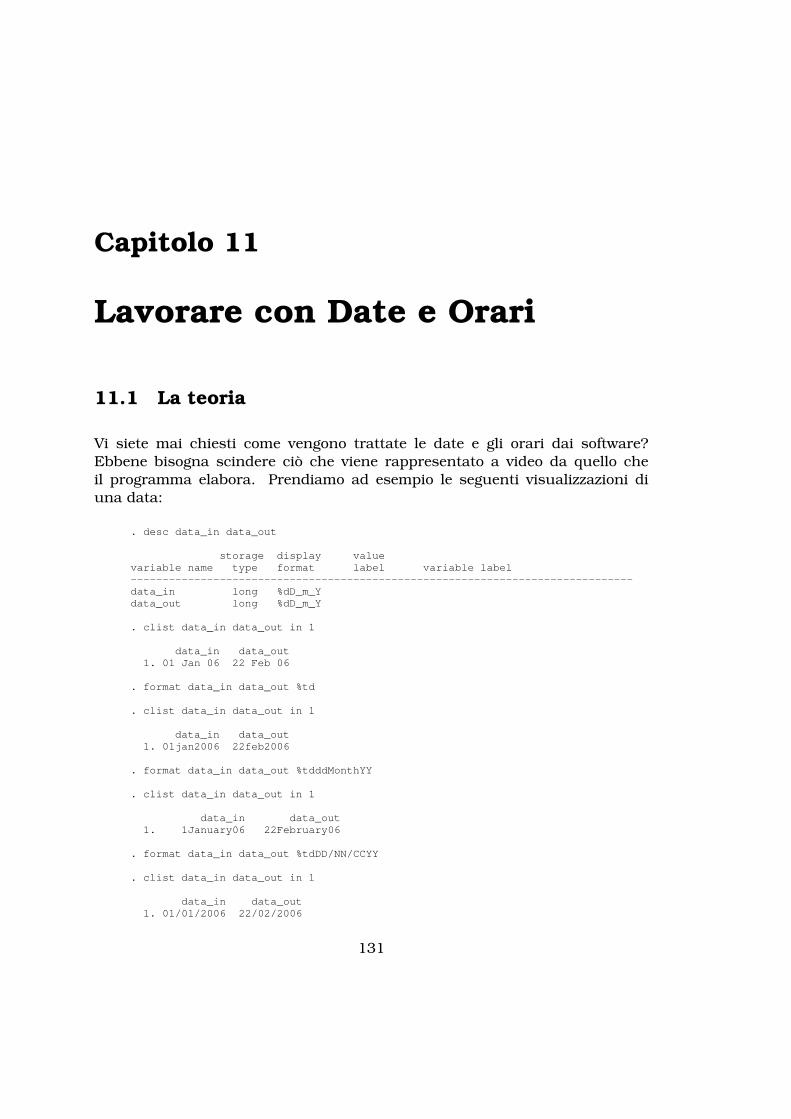
Capitolo 11
Lavorare con Date e Orari
11.1 La teoria
Vi siete mai chiesti come vengono trattate le date e gli orari dai software?Ebbene bisogna scindere ciò che viene rappresentato a video da quello cheil programma elabora. Prendiamo ad esempio le seguenti visualizzazioni diuna data:
. desc data_in data_out
storage display valuevariable name type format label variable label-------------------------------------------------------------------------------data_in long %dD_m_Ydata_out long %dD_m_Y
. clist data_in data_out in 1
data_in data_out1. 01 Jan 06 22 Feb 06
. format data_in data_out %td
. clist data_in data_out in 1
data_in data_out1. 01jan2006 22feb2006
. format data_in data_out %tdddMonthYY
. clist data_in data_out in 1
data_in data_out1. 1January06 22February06
. format data_in data_out %tdDD/NN/CCYY
. clist data_in data_out in 1
data_in data_out1. 01/01/2006 22/02/2006
131

11.1. La teoria 11. Lavorare con Date e Orari
Come vedete ci sono diverse visualizzazioni della stessa informazione che inrealtà è un numero intero:
. summ data_in data_out in 1
Variable | Obs Mean Std. Dev. Min Max-------------+--------------------------------------------------------
data_in | 1 16802 . 16802 16802data_out | 1 16854 . 16854 16854
Infatti il meccanismo si basa sull’assegnazione alla data del 01/01/1960 delvalore 0, al 02/01/1960 del valore 1 e così via. Quindi il calcolo dei giorni tradue date si riduce ad una differenza tra due numeri interi. La stessa logicasi applica ai dati rigurdanti le ore. In questo caso si ragiona in termine dimillisecondi (ms) a partire dalle ore 0, 0 minuti, 0 secondi e 0 millisecondi del1 gennaio 1960. Per i calcoli si considerino le seguenti equivalenze:
- 1 secondo = 1000ms- 1 minuto = 60sec × 1000ms = 60000ms- 1 ora = 60min × 60sec × 1000ms = 3600000ms- 1 giorno = 24h × 60min × 60sec × 1000ms = 86400000ms
E per date e ore antecedenti il primo gennaio 1960? Ovviamente si ricorre anumeri interi negativi!In Stata sono possibili diversi sistemi di misura e a partire dalla versione 10è stata introdotta anche la possibilità di usare la misura basata sulle ore. Aseconda del formato che associamo al dato avremo le seguenti interpretazioni:
Formato Rappresenta Valore -1 Valore 0 Valore 1
%tc orario 31 Dicembre1959
23:59:59:999
1 Gennaio1960
00:00:00:000
1 Gennaio1960
00:00:00:001
%tC orario 31 Dicembre1959
23:59:59:999
1 Gennaio1960
00:00:00:000
1 Gennaio1960
00:00:00:001
%td giorni 31 Dicembre1959
1 Gennaio1960
1 Gennaio1960
%tw settimane 1959settimana 52
1960settimana 1
1960settimana 2
%tm mesi 1959 dicembre 1960 gennaio 1960 febbraio
132 Nicola Tommasi

11. Lavorare con Date e Orari 11.1. La teoria
%tq quadrimestri 1959 quartoquadrimestre
1960 primoquadrimestre
1960 secondoquadrimestre
%th semestri 1959 secondosemestre
1960 primosemestre
1960 secondosemestre
%ty anni 1 ac 0 1 dc
%tg generico -1 0 1
Vediamo adesso a cosa corripondono i valori di var1 in formato %tc e %tC:
. gen double var2 = var1
. format var2 %tc
. gen double var3 = var1
. format var3 %tC
. clist
var1 var2 var31. -100000 31dec1959 23:58:20 31dec1959 23:58:202. 0 01jan1960 00:00:00 01jan1960 00:00:003. 100 01jan1960 00:00:00 01jan1960 00:00:004. 1000 01jan1960 00:00:01 01jan1960 00:00:015. 10000 01jan1960 00:00:10 01jan1960 00:00:106. 100000 01jan1960 00:01:40 01jan1960 00:01:407. 100000000 02jan1960 03:46:40 02jan1960 03:46:408. 100000000000 03mar1963 09:46:40 03mar1963 09:46:40
A questo punto spieghiamo la differenza tra %tc e %tC. Le due configurazionisono uguali eccetto per il fatto che %tC tiene conto anche dei secondi inseritiin seguito a correzioni astronomiche per la sincronizzazione con la rotazionedella terra (standard GMT). Invece %tc si basa sull’orologio atomico (standardUTC).Per completare il quadro vediamo i valori dei rimanenti %t per diversi valori divar1:
. gen var4 = var1
. format var4 %td
. gen var5 = var1
. gen var5 = var1
. format var5 %tw
. gen var6 = var1
. format var6 %tm
Nicola Tommasi 133
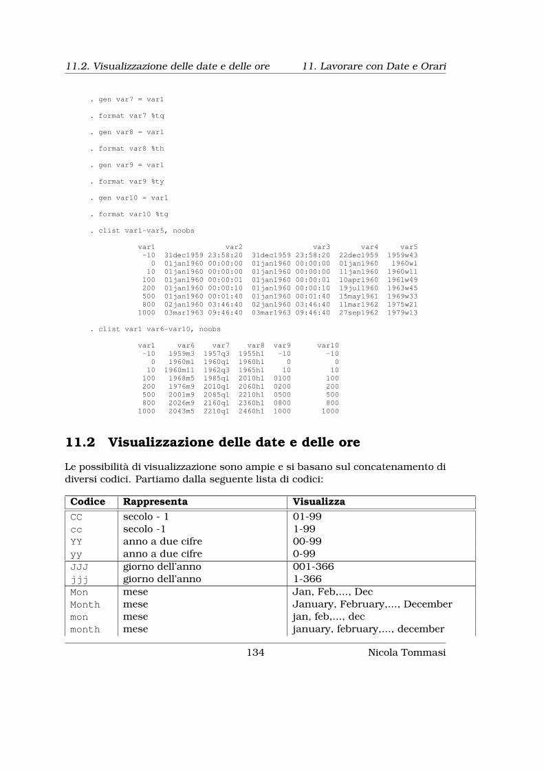
11.2. Visualizzazione delle date e delle ore 11. Lavorare con Date e Orari
. gen var7 = var1
. format var7 %tq
. gen var8 = var1
. format var8 %th
. gen var9 = var1
. format var9 %ty
. gen var10 = var1
. format var10 %tg
. clist var1-var5, noobs
var1 var2 var3 var4 var5-10 31dec1959 23:58:20 31dec1959 23:58:20 22dec1959 1959w430 01jan1960 00:00:00 01jan1960 00:00:00 01jan1960 1960w110 01jan1960 00:00:00 01jan1960 00:00:00 11jan1960 1960w11100 01jan1960 00:00:01 01jan1960 00:00:01 10apr1960 1961w49200 01jan1960 00:00:10 01jan1960 00:00:10 19jul1960 1963w45500 01jan1960 00:01:40 01jan1960 00:01:40 15may1961 1969w33800 02jan1960 03:46:40 02jan1960 03:46:40 11mar1962 1975w211000 03mar1963 09:46:40 03mar1963 09:46:40 27sep1962 1979w13
. clist var1 var6-var10, noobs
var1 var6 var7 var8 var9 var10-10 1959m3 1957q3 1955h1 -10 -100 1960m1 1960q1 1960h1 0 010 1960m11 1962q3 1965h1 10 10100 1968m5 1985q1 2010h1 0100 100200 1976m9 2010q1 2060h1 0200 200500 2001m9 2085q1 2210h1 0500 500800 2026m9 2160q1 2360h1 0800 8001000 2043m5 2210q1 2460h1 1000 1000
11.2 Visualizzazione delle date e delle ore
Le possibilità di visualizzazione sono ampie e si basano sul concatenamento didiversi codici. Partiamo dalla seguente lista di codici:
Codice Rappresenta VisualizzaCC secolo - 1 01-99cc secolo -1 1-99YY anno a due cifre 00-99yy anno a due cifre 0-99JJJ giorno dell’anno 001-366jjj giorno dell’anno 1-366Mon mese Jan, Feb,..., DecMonth mese January, February,..., Decembermon mese jan, feb,..., decmonth mese january, february,..., december
134 Nicola Tommasi

11. Lavorare con Date e Orari 11.2. Visualizzazione delle date e delle ore
Codice Rappresenta VisualizzaNN mese 01-12nn mese 1-12DD giorno del mese 01-31dd giorno del mese 1-31DAYNAME giorno della settimana Sunday, Monday, ... (allineato?)Dayname giorno della settimana Sunday, Monday, ... (non allineato?)Day giorno della settimana Sun, Mon,...Da giorno della settimana Su, mo,...day giorno della settimana sun, mon,...da giorno della settimana su, mo,...h semestre 1-2q quadrimestre 1-4WW settimana 01-52ww settimana 1-52HH ora 00-23Hh ora 00-12hH ora 0-23hh ora 0-12MM minuti 00-59mm minuti 0-59SS secondi 00-60ss secondi 0-60.s decimi .0-.9.ss centesimi .00-.99.sss millesimi .000-.999am visualizza am o pm am o pma.m. visualizza a.m. o p.m. a.m. o p.m.AM visualizza AM o PM AM o PMA.M. visualizza A.M. o P.M. A.M. o P.M.. visualizza un punto ., visualizza una virgola ,: visualizza i due punti :- visualizza un trattino -_ visualizza uno spazio/ visualizza la barra inclinata a dx /\ visualizza la barra inclinata a sx \!tc visualizza il carattere c c+ separatore della sintassi1
1Serve solo a separare i vari codici affinché siano più leggibili, ma non ha nessun effetto suquanto visualizzato
Nicola Tommasi 135
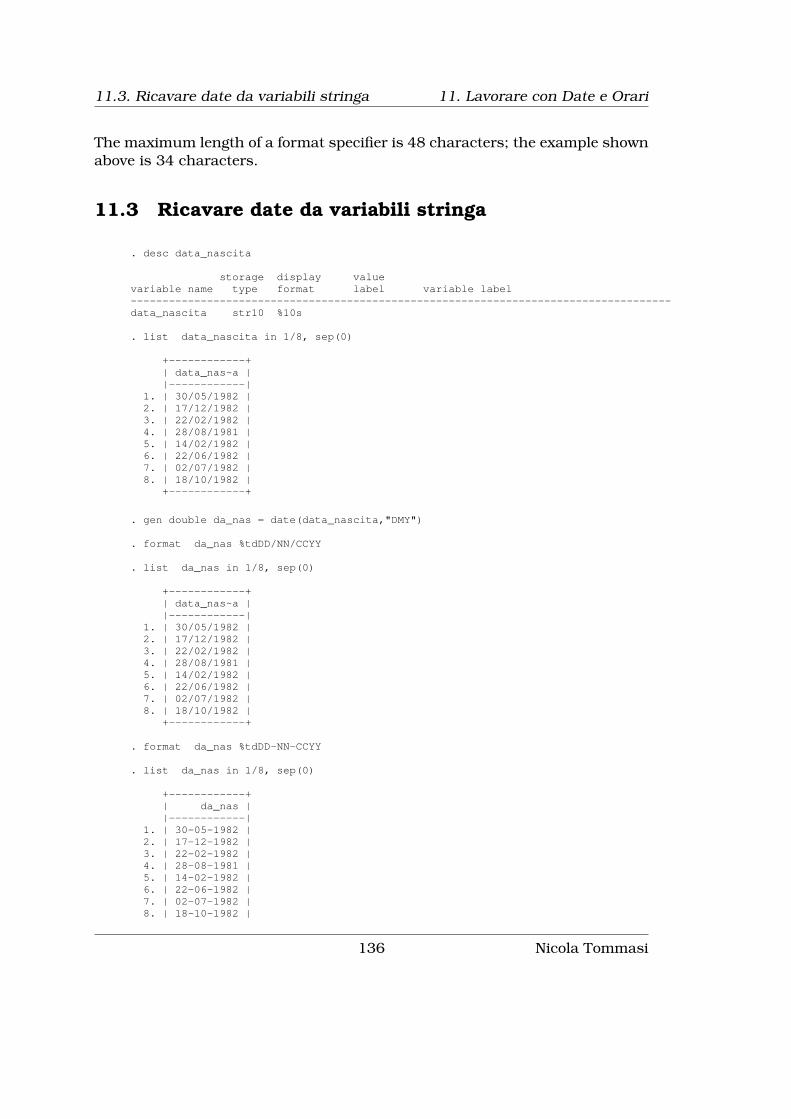
11.3. Ricavare date da variabili stringa 11. Lavorare con Date e Orari
The maximum length of a format specifier is 48 characters; the example shownabove is 34 characters.
11.3 Ricavare date da variabili stringa
. desc data_nascita
storage display valuevariable name type format label variable label-------------------------------------------------------------------------------------data_nascita str10 %10s
. list data_nascita in 1/8, sep(0)
+------------+| data_nas~a ||------------|
1. | 30/05/1982 |2. | 17/12/1982 |3. | 22/02/1982 |4. | 28/08/1981 |5. | 14/02/1982 |6. | 22/06/1982 |7. | 02/07/1982 |8. | 18/10/1982 |
+------------+
. gen double da_nas = date(data_nascita,"DMY")
. format da_nas %tdDD/NN/CCYY
. list da_nas in 1/8, sep(0)
+------------+| data_nas~a ||------------|
1. | 30/05/1982 |2. | 17/12/1982 |3. | 22/02/1982 |4. | 28/08/1981 |5. | 14/02/1982 |6. | 22/06/1982 |7. | 02/07/1982 |8. | 18/10/1982 |
+------------+
. format da_nas %tdDD-NN-CCYY
. list da_nas in 1/8, sep(0)
+------------+| da_nas ||------------|
1. | 30-05-1982 |2. | 17-12-1982 |3. | 22-02-1982 |4. | 28-08-1981 |5. | 14-02-1982 |6. | 22-06-1982 |7. | 02-07-1982 |8. | 18-10-1982 |
136 Nicola Tommasi

11. Lavorare con Date e Orari 11.4. Visualizzazione delle ore
+------------+
11.4 Visualizzazione delle ore
11.5 Operazioni con date e ore
Nicola Tommasi 137


Capitolo 12
Macros e Cicli
12.1 Macros
In Stata esistono due tipi di macros: local e global. La distinzione tra ledue è attinente alla programmazione per cui in questa sede le possiamo con-siderare come equivalenti. La loro funzione è quella di un contenitore in cuiinserire numeri o stringhe da richiamare in un secondo momento. I modi perassegnare un contenuto sono diversi e comunque prevedono l’assegnazione diun nome. Per evitare problemi meglio scegliere nomi diversi da quelli assegnatialle variabili.
local A 2+2local A = 2+2local B "hello world"local B = "hello world"
global A 2+2global A = 2+2global B "hello world"global B = "hello world"
Si vede che è possibile assegnare il contenuto alla macro sia con il segno = chesenza. La differenza è sostanziale quando si assegnano valori o espressioninumeriche. Vediamo un esempio:
. local A 2+2
. local B = 2+2
. di `A'4
. di `B'4
. di "`A'"2+2
. di "`B'"4
139

12.1. Macros 12. Macros e Cicli
Con local A 2+2 sto’ assegnano ad A 2+2, che sarà interpretato come op-erazione algebrica se lo uso direttamente (di `A'), come stringa se lo usocon (di `A'). Con local B = 2+2 invece sarà sempre interpretato come op-erazione algebrica. È importante essere a conoscenza di questa differenza nelmomento in cui si richiamano le macros create perché sono diversi i contenutidi A. Stesso discorso vale per le global.
Vediamo ora come richiamare le macros:
- le local si richiamano con l'espressione `local_name'- le global si richiamano con l'espressione $local_name
il simbolo ` si ottiene premendo ALT + 96 sul tastierino numerico
Adesso vediamo qualche uso pratico. Per esempio possiamo definire una listadi variabili da utilizzare successivamente in diverse situazioni:
local list = "inc2001 inc2000 inc1999 inc1998 inc1997 inc1996 inc1995"
. di "`list'inc2001 inc2000 inc1999 inc1998 inc1997 inc1996 inc1995
. summ `list'
Variable | Obs Mean Std. Dev. Min Max-------------+--------------------------------------------------------
inc2001 | 1460 32961.99 44469.03 0 480000inc2000 | 1476 32833.82 44145.67 0 600000inc1999 | 1393 31891.78 41724.69 0 480000inc1998 | 1400 31550.77 40743.81 0 410000inc1997 | 1369 31438.15 37784.66 0 350000
-------------+--------------------------------------------------------inc1996 | 1364 32373.4 40198.93 0 600000inc1995 | 1413 30598.08 36889.4 0 360000
. regress inc2002 `list'
Source | SS df MS Number of obs = 1328-------------+------------------------------ F( 7, 1320) = 745.90
Model | 2.2244e+12 7 3.1777e+11 Prob > F = 0.0000Residual | 5.6234e+11 1320 426018392 R-squared = 0.7982
-------------+------------------------------ Adj R-squared = 0.7971Total | 2.7867e+12 1327 2.1000e+09 Root MSE = 20640
------------------------------------------------------------------------------inc2002 | Coef. Std. Err. t P>|t| [95% Conf. Interval]
-------------+----------------------------------------------------------------inc2001 | .8007813 .0340487 23.52 0.000 .7339858 .8675769inc2000 | .1072529 .0472282 2.27 0.023 .0146023 .1999035inc1999 | .0850962 .0556251 1.53 0.126 -.024027 .1942195inc1998 | -.0983748 .0463245 -2.12 0.034 -.1892526 -.0074971inc1997 | .1441902 .0399267 3.61 0.000 .0658633 .222517inc1996 | -.1652574 .0452349 -3.65 0.000 -.2539975 -.0765173inc1995 | .0531481 .0438402 1.21 0.226 -.0328559 .1391521_cons | 3392.282 755.4408 4.49 0.000 1910.286 4874.278
------------------------------------------------------------------------------
140 Nicola Tommasi

12. Macros e Cicli 12.2. I cicli
Vedremo tra poco come utilizzare le local all’interno dei cicli e successiva-mente come usarle per catturare e riutilizzare l’output dei comandi.Vediamo però anche come utilizzare un altro oggetto chiamato scalar. Essoserve per assegnare valori numerici scalari e si costruisce così:
scalar[define
]scalar_name =exp
. scalar w=5
. scalar q=3
. scalar t=w+q
. di t8
12.2 I cicli
I cicli sono delle procedure che permettono di compiere azioni ripetitive inmaniera più veloce ed efficiente usando poche righe di codice. I metodi di im-plementazione sono diversi a seconda del contesto in cui si vogliono utilizzare.Analizziamo adesso il metodo foreach la cui sintassi generale è:
foreach lname {in|of listtype} list {
commands referring to `lname'
}
in pratica succederà che di volta in volta tutti gli oggetti specificati in listverranno assegnati a lname e quindi eseguiti in base alla lista di comandispecificata tra le due parentesi graffe (commands referring to `lname').Sono possibili le seguenti costruzioni di foreach:I costruzione
foreach lname in any_list {
.... lista di comandi
}
È la costruzione più generale e in any_list possiamo inserire una qualsiasi lista:nomi di variabili, stringhe e numeri.
II costruzione
foreach lname of local lmacname {
.... lista di comandi
}
previa specificazione del contenuto di una local lmacname, possiamo utiliz-zare il suo contenuto in questo tipo di ciclo.
Nicola Tommasi 141

12.2. I cicli 12. Macros e Cicli
III costruzione
foreach lname of global gmacname {
.... lista di comandi
}
previa specificazione del contenuto di una global gmacname, possiamo utiliz-zare il suo contenuto in questo tipo di ciclo.
IV costruzione
foreach lname of varlist varlist {
.... lista di comandi
}
utilizzeremo questa costruzione solo quando faremo riferimento ad una seriedi variabili già esistenti.
V costruzione
foreach lname of newvarlist newvarlist {
.... lista di comandi
}
costruzione poco usata dove in newvarlist si indica una lista di nuove variabiliche verranno create all’interno del ciclo
VI costruzione
foreach lname of numlist numlist {
.... lista di comandi
}
che consente di sfruttare le proprietà delle numlist di Stata (che vedremo trapoco).
Per capire meglio vediamo alcuni esempi. Per la prima costruzione:
. foreach obj in var1 var2 var8 var10 {2. summ `obj'3. gen `obj'_10 = `obj' / 104. summ `obj'_105. }
Variable | Obs Mean Std. Dev. Min Max-------------+--------------------------------------------------------
var1 | 888 .4868541 .2868169 .0003254 .9990993
Variable | Obs Mean Std. Dev. Min Max-------------+--------------------------------------------------------
var1_10 | 888 .0486854 .0286817 .0000325 .0999099
Variable | Obs Mean Std. Dev. Min Max
142 Nicola Tommasi

12. Macros e Cicli 12.2. I cicli
-------------+--------------------------------------------------------var2 | 888 .4839523 .2927765 .004523 .9999023
Variable | Obs Mean Std. Dev. Min Max-------------+--------------------------------------------------------
var2_10 | 888 .0483952 .0292776 .0004523 .0999902
Variable | Obs Mean Std. Dev. Min Max-------------+--------------------------------------------------------
var8 | 888 .4880482 .2916573 .0005486 .9985623
Variable | Obs Mean Std. Dev. Min Max-------------+--------------------------------------------------------
var8_10 | 888 .0488048 .0291657 .0000549 .0998562
Variable | Obs Mean Std. Dev. Min Max-------------+--------------------------------------------------------
var10 | 888 .5048937 .2783813 .003708 .9995353
Variable | Obs Mean Std. Dev. Min Max-------------+--------------------------------------------------------
var10_10 | 888 .0504894 .0278381 .0003708 .0999535
quello che accade è che ad ogni ciclo in obj viene sostituita in sequenza var1,var2, var8 e infine var10 in questa maniera:
primo ciclo (‘obj’ = var1):summ ‘obj’ summ var1gen ‘obj’_10 = ‘obj’ / 10 gen var1_10 = var1 / 10summ ‘obj’_10 summ var1_10
secondo ciclo (‘obj’ = var2):summ ‘obj’ summ var2gen ‘obj’_10 = ‘obj’ / 10 gen var2_10 = var2 / 10summ ‘obj’_10 summ var2_10
terzo ciclo (‘obj’ = var8):summ ‘obj’ summ var8gen ‘obj’_10 = ‘obj’ / 10 gen var8_10 = var8 / 10summ ‘obj’_10 summ var8_10
quarto e ultimo ciclo (‘obj’ = var10):summ ‘obj’ summ var10gen ‘obj’_10 = ‘obj’ / 10 gen var10_10 = var10 / 10summ ‘obj’_10 drop var10_10
Vediamo ora un esempio per la seconda costruzione. Per prima cosa dobbiamodefinire la local e poi rifacciamo lo stesso ciclo:
local lista = "var1 var2 var8 var10"
. foreach obj of local lista {2. summ `obj'
Nicola Tommasi 143

12.2. I cicli 12. Macros e Cicli
3. gen `obj'_10 = `obj' / 104. summ `obj'_105. }
(output omitted ) ... tanto è uguale al precedente
Si noti che la local all’interno del ciclo foreach viene richiamata SENZA l’usodegli apostrofi.
Per la terza costruzione definiamo la global
. global lista = "var1 var2 var8 var10"
. foreach obj of global lista {2. summ `obj'3. gen `obj'_10 = `obj' / 104. summ `obj'_105. }
(output omitted ) ... idem come sopra
Anche qui è da notare che la global viene richiamata senza il simbolo $davanti.
Per la quarta costruzione possiamo sfruttare le possibilità offerte da Stata inmerito alla selezione delle variabili su cui eseguire i comandi:
. foreach obj of varlist var? {2. summ `obj'3. gen `obj'_10 = `obj' / 104. summ `obj'_105. }
Variable | Obs Mean Std. Dev. Min Max-------------+--------------------------------------------------------
var1 | 888 .4868541 .2868169 .0003254 .9990993
Variable | Obs Mean Std. Dev. Min Max-------------+--------------------------------------------------------
var1_10 | 888 .0486854 .0286817 .0000325 .0999099
Variable | Obs Mean Std. Dev. Min Max-------------+--------------------------------------------------------
var2 | 888 .4839523 .2927765 .004523 .9999023
Variable | Obs Mean Std. Dev. Min Max-------------+--------------------------------------------------------
var2_10 | 888 .0483952 .0292776 .0004523 .0999902
Variable | Obs Mean Std. Dev. Min Max-------------+--------------------------------------------------------
var8 | 888 .4880482 .2916573 .0005486 .9985623
Variable | Obs Mean Std. Dev. Min Max-------------+--------------------------------------------------------
var8_10 | 888 .0488048 .0291657 .0000549 .0998562
Notare che var10 non viene considerata perchè non rientra in var?. Tralas-ciando la quinta costruzione, vediamo un esempio della sesta, annidandolaperò all’interno di un altro ciclo (ebbene sì, i cicli possono essere inseritiall’interno di altri cicli):
144 Nicola Tommasi

12. Macros e Cicli 12.2. I cicli
. foreach obj of varlist var1? {2. foreach expo of numlist 2/4 6 {3. gen `obj'_`expo' = `obj'^(`expo')4. }5. summ `obj'_*6. }
Variable | Obs Mean Std. Dev. Min Max-------------+--------------------------------------------------------
var10_2 | 888 .3323266 .286364 .0000137 .9990708var10_3 | 888 .2448896 .2705386 5.10e-08 .9986064var10_4 | 888 .1923529 .2533452 1.89e-10 .9981424var10_6 | 888 .1330797 .224473 2.60e-15 .9972148
Variable | Obs Mean Std. Dev. Min Max-------------+--------------------------------------------------------
var11_2 | 888 .3293853 .2923062 1.48e-06 .9904835var11_3 | 888 .2443889 .2775777 1.80e-09 .9857593var11_4 | 888 .1938413 .2602036 2.19e-12 .9810576var11_6 | 888 .1366885 .229854 3.24e-18 .9717214
Variable | Obs Mean Std. Dev. Min Max-------------+--------------------------------------------------------
var12_2 | 888 .341181 .3057852 9.02e-07 .9987798var12_3 | 888 .2591221 .2929291 8.56e-10 .9981703var12_4 | 888 .2098038 .2770279 8.13e-13 .997561var12_6 | 888 .1528551 .2492659 7.33e-19 .9963439
In pratica per ciascuna variabile il cui nome inizia var1# viene costruita unavariabile con la sua trasformazione al quadrato, al cubo, alla quarta e allasesta. Anche in questo caso esaminiamo la successione delle operazioni:
primo loop del ciclo principale (‘obj’ = var10)primo loop del ciclo annidato (‘expo’ = 2)
gen ‘obj’_‘expo’ = ‘obj’^(‘expo’) gen var10_2 = var10^(2)
secondo loop ciclo annidato (‘expo’ = 3)gen ‘obj’_‘expo’ = ‘obj’^(‘expo’) gen var10_3 = var10^(3)
terzo loop ciclo annidato (‘expo’ = 4)gen ‘obj’_‘expo’ = ‘obj’^(‘expo’) gen var10_4 = var10^(4)
quarto loop ciclo annidato (‘expo’ = 6)gen ‘obj’_‘expo’ = ‘obj’^(‘expo’) gen var10_6 = var10^(6)
chiusura loop del ciclo annidatosumm ‘obj’_* summ var10_*
secondo loop del ciclo principale (‘obj’ = var11)primo loop del ciclo annidato (‘expo’ = 2)
gen ‘obj’_‘expo’ = ‘obj’^(‘expo’) gen var11_2 = var11^(2)
Nicola Tommasi 145
12.2. I cicli 12. Macros e Cicli
secondo loop ciclo annidato (‘expo’ = 3)gen ‘obj’_‘expo’ = ‘obj’^(‘expo’) gen var11_3 = var11^(3)
terzo loop ciclo annidato (‘expo’ = 4)gen ‘obj’_‘expo’ = ‘obj’^(‘expo’) gen var11_4 = var11^(4)
quarto loop ciclo annidato (‘expo’ = 6)gen ‘obj’_‘expo’ = ‘obj’^(‘expo’) gen var11_6 = var11^(6)
chiusura loop del ciclo annidatosumm ‘obj’_* summ var11_*
terzo loop del ciclo principale (‘obj’ = var12)primo loop del ciclo annidato (‘expo’ = 2)
gen ‘obj’_‘expo’ = ‘obj’^(‘expo’) gen var12_2 = var12^(2)
secondo loop ciclo annidato (‘expo’ = 3)gen ‘obj’_‘expo’ = ‘obj’^(‘expo’) gen var12_3 = var12^(3)
terzo loop ciclo annidato (‘expo’ = 4)gen ‘obj’_‘expo’ = ‘obj’^(‘expo’) gen var12_4 = var12^(4)
quarto loop ciclo annidato (‘expo’ = 6)gen ‘obj’_‘expo’ = ‘obj’^(‘expo’) gen var12_6 = var12^(6)
chiusura loop del ciclo annidatosumm ‘obj’_* summ var12_*
Infine esiste un’altra costruzione da usare però solo con serie numeriche:
forvalues lname = range {
commands referring to `lname'
}
dove range può assumere le seguenti configurazioni:
- #1(#d)#2: lname assume valori da #1 a #2 con passo pari a #d- #1/#2: lname assume valori da #1 a #2 con passo pari a 1- #1 (#t) to #2: lname assume valori da #1 a #2 con passo pari a #t - #1- #1 (#t) : #2: idem come sopra
Un esempio:
forvalues n = 1(1)90 {replace var`n' = var`n' + alvar`n'}
che esegue il replace su sulle 90 variabili var1, var2, ...., var90.
146 Nicola Tommasi

Capitolo 13
Catturare Informazioni dagliOutput
Ogni volta che eseguite un comando, Stata salva parte dell’output del comandoe altri valori che vengono calcolati durante l’esecuzione in particolari localche possono essere richiamate ed utilizzate. Il comando per vedere l’elenco deirisultati salvati è return list:
. summ price
Variable | Obs Mean Std. Dev. Min Max-------------+--------------------------------------------------------
price | 74 6165.257 2949.496 3291 15906
. return list
scalars:r(N) = 74
r(sum_w) = 74r(mean) = 6165.256756756757r(Var) = 8699525.974268789r(sd) = 2949.495884768919r(min) = 3291r(max) = 15906r(sum) = 456229
. summ price, detail
Price-------------------------------------------------------------
Percentiles Smallest1% 3291 32915% 3748 329910% 3895 3667 Obs 7425% 4195 3748 Sum of Wgt. 74
50% 5006.5 Mean 6165.257Largest Std. Dev. 2949.496
75% 6342 1346690% 11385 13594 Variance 869952695% 13466 14500 Skewness 1.65343499% 15906 15906 Kurtosis 4.819188
147

13. Catturare Informazioni dagli Output
. return list
scalars:r(N) = 74
r(sum_w) = 74r(mean) = 6165.256756756757r(Var) = 8699525.97426879r(sd) = 2949.49588476892
r(skewness) = 1.653433511704859r(kurtosis) = 4.819187528464004
r(sum) = 456229r(min) = 3291r(max) = 15906r(p1) = 3291r(p5) = 3748r(p10) = 3895r(p25) = 4195r(p50) = 5006.5r(p75) = 6342r(p90) = 11385r(p95) = 13466r(p99) = 15906
Invece nel caso di una regressione si deve usare ereturn list:
. regress price mpg rep78 weight length foreign
Source | SS df MS Number of obs = 69-------------+------------------------------ F( 5, 63) = 15.90
Model | 321789308 5 64357861.7 Prob > F = 0.0000Residual | 255007650 63 4047740.48 R-squared = 0.5579
-------------+------------------------------ Adj R-squared = 0.5228Total | 576796959 68 8482308.22 Root MSE = 2011.9
------------------------------------------------------------------------------price | Coef. Std. Err. t P>|t| [95% Conf. Interval]
-------------+----------------------------------------------------------------mpg | -26.01325 75.48927 -0.34 0.732 -176.8665 124.84
rep78 | 244.4242 318.787 0.77 0.446 -392.6208 881.4691weight | 6.006738 1.03725 5.79 0.000 3.93396 8.079516length | -102.2199 34.74826 -2.94 0.005 -171.6587 -32.78102foreign | 3303.213 813.5921 4.06 0.000 1677.379 4929.047_cons | 5896.438 5390.534 1.09 0.278 -4875.684 16668.56
------------------------------------------------------------------------------
. ereturn list
scalars:e(N) = 69
e(df_m) = 5e(df_r) = 63
e(F) = 15.8997005734978e(r2) = .5578900919500578
e(rmse) = 2011.899719996595e(mss) = 321789308.4202555e(rss) = 255007650.4493099e(r2_a) = .5228020040095862e(ll) = -619.6398259855126
e(ll_0) = -647.7986144493904
macros:e(cmdline) : "regress price mpg rep78 weight length foreign"e(title) : "Linear regression"e(vce) : "ols"
e(depvar) : "price"
148 Nicola Tommasi

13. Catturare Informazioni dagli Output
e(cmd) : "regress"e(properties) : "b V"
e(predict) : "regres_p"e(model) : "ols"
e(estat_cmd) : "regress_estat"
matrices:e(b) : 1 x 6e(V) : 6 x 6
functions:e(sample)
Ritornando al primo esempio, tutti gli r() sono dei risultati che possiamorichiamare all’interno dei comandi o che possiamo salvare in local. Infattibisogna tener presente che i valori salvati in r() cambiano dopo l’esecuzionedel comando e contengono solo quelli relativi all’ultimo comando eseguito.Se per esempio voglio costruire una variabile (var3) che sia la moltiplicazionedi una variabile (var2) per la media di un’altra (var1), dovrò fare:
. summ var2
Variable | Obs Mean Std. Dev. Min Max-------------+--------------------------------------------------------
var2 | 88 .5022995 .2882645 .0057233 .9844069
. summ var1
Variable | Obs Mean Std. Dev. Min Max-------------+--------------------------------------------------------
var1 | 88 .4676347 .2849623 .0369273 .9763668
. return list
scalars:r(N) = 88
r(sum_w) = 88r(mean) = .4676347244530916r(Var) = .0812035311082154r(sd) = .284962332788415r(min) = .0369273088872433r(max) = .9763667583465576r(sum) = 41.15185575187206
. gen var3 = var2 * r(mean)
. summ var3
Variable | Obs Mean Std. Dev. Min Max-------------+--------------------------------------------------------
var3 | 88 .2348927 .1348025 .0026764 .4603429
Oppure se voglio salvare in una local la sommatoria di una variabile
. summ var1
Variable | Obs Mean Std. Dev. Min Max-------------+--------------------------------------------------------
var1 | 88 .4676347 .2849623 .0369273 .9763668
. return list
Nicola Tommasi 149
13. Catturare Informazioni dagli Output
scalars:r(N) = 88
r(sum_w) = 88r(mean) = .4676347244530916r(Var) = .0812035311082154r(sd) = .284962332788415r(min) = .0369273088872433r(max) = .9763667583465576r(sum) = 41.15185575187206
. local sommatoria_var1 = r(sum)
. di `sommatoria_var1'41.151856
150 Nicola Tommasi

Capitolo 14
Mappe
Ora anche in Stata è possibile rappresentare i dati su base geografica (geo-referenziazione) grazie all’ottimo lavoro di Maurizio Pisati tramite il comandospmap. Per prima cosa bisogna procurarsi i dati geografici che in genere viverranno forniti in uno dei due formati che sono standard di fatto: shape filee MapInfo Interchange Format. Per poterli utilizzare con spmap occorre con-vertirli in database di Stata. Gli shape file vengono convertiti attraverso ilcomando
shp2dta using shpfilename , database(filename) coordinates(filename)[replace genid(newvarname) gencentroids(stub)
]dove:
shpfilename è il file con estensione .shpdatabase(filename) è il nome del nuovo dataset di Stata che conterrà le in-
formazioni del .dbf file.coordinates(filename) è il nome del nuovo dataset di Stata che conterrà le
informazioni dello .shp file ovvero le coordinate per disegnare i confinidegli oggetti da rappresentare.
replace sovrascrive i file specificati in database(filename) e in coordinates(filename).genid(newvarname) specifica il nome di una nuova variabile in database(filename)
che sarà un identificativo delle diverse aree geografiche. I valori assuntida questa variabile corrispondono a quelli della variabile _ID presente nelfile coordinates(filename).
gencentroids(stub) genera le variabili x_stub e y_stub in database(filename)che contengono le coordinate dei centroidi delle aree geografiche.
I files MapInfo sono solitamente due con lo stesso nome ma uno con estensione.mif che contiene le coordinate dei poligoni da disegnare e l’altro con estensione.mid che contiene i dati riferiti alle aree geografiche. Il comando per convertirequesto tipo di dati è
mif2dta rootname, genid(newvarname)[gencentroids(stub)
]151

14. Mappe
dove:
rootname è il nome comune dei due files .mif e .midgenid(newvarname) specifica il nome di una nuova variabile che sarà un
identificativo delle diverse aree geografiche.gencentroids(stub) genera le variabili x_stub e y_stub in che contengono
le coordinate dei centroidi delle aree geografiche.
Il comando genera due database .dta: rootname-Database.dta e rootname-Coordinates.dta.
Bene! Ora abbiamo i files in formato Stata e pronti ad essere utilizzati con ilcomando spmap per la rappresentazione geografica. spmap è veramente riccodi opzioni per cui ho riportato l’help del comando in Appendice (pag. 193)assieme ad alcuni esempi grafici. Qui si discuterà di alcuni aspetti inerentil’utilizzo. Le coordinate dei centroidi non sempre sono corrette nel posizionaregli elementi che si vogliono rappresentare al centro dell’area geografica percui bisogna correggerli. Questa operazione non è difficile dato che si basanosu coordinate cartesiane, comunque bisogna investirci un po’ di tempo. Eccoun esempio pratico in cui si riportano le iniziali dei comuni della provincia diVerona, prima senza e poi con la correzione delle coordinate dei centroidi.
. local PR "vr";
. /*** conversione shape file nel formato voluto da Stata per il comando spmap***/;
. shp2dta using `PR'_comuni.shp, database(`PR') coordinates(`PR'_coord)> replace genid(ID) gencentroids(c);
. use `PR'.dta, clear;
. rename ID _ID;
. spmap sup using "`PR'_coord", id(_ID) fcolor(Blues2) clnumber(98) ocolor(white ..)> label(label(nom_com_abb) x(x_c) y(y_c) size(1.5) )> legenda(off) title("`sch'", size(*0.8));
. graph export map_pre.png, replace;(note: file map_pre.png not found)(file map_pre.png written in PNG format)
e questa è la mappa risultante.OK, adesso la serie di correzioni delle coordinate e il relativo risultato
. replace y_c=y_c + 1100 if cod_com==30;(1 real change made)
. replace x_c=x_c - 800 if cod_com==30;(1 real change made)
. replace y_c=y_c - 400 if cod_com==36;(1 real change made)
. replace x_c=x_c + 1000 if cod_com==36;(1 real change made)
152 Nicola Tommasi

14. Mappe
Figura 14.1: Mappa pre correzione
Nicola Tommasi 153

14. Mappe
(output omitted )
. replace y_c=y_c + 400 if cod_com==10;(1 real change made)
. replace y_c=y_c - 600 if cod_com==56;(1 real change made)
. replace x_c=x_c + 400 if cod_com==26;(1 real change made)
. replace y_c=y_c - 1800 if cod_com==38;(1 real change made)
. spmap sup using "`PR'_coord", id(_ID) fcolor(Blues2) clnumber(98) ocolor(white ..)> label(label(nom_com_abb) x(x_c) y(y_c) size(1.5) )> legenda(off) title("`sch'", size(*0.8));
. graph export map_post.png, replace;(note: file map_post.png not found)(file map_post.png written in PNG format)
Altro problema. Quando si rappresentano dati continui attraverso una choro-pleth map usando una delle combinazioni di colori previste dal programma,se c’è del testo da rappresentare ci può essere un problema di visualizzazione.Ovvero se il testo è di colore chiaro sarà difficilmente leggibile nelle aree piùchiare, viceversa se il testo è di colore scuro sarà difficilmente leggibile nellearee più scure. Potete apprezzare quanto appena detto nella figura prodottada questo codice
. local tit : variable label pedia_od;
. spmap pedia_odp using coord_ulss.dta, id(_ID) fcolor(Blues2) ocolor(black ..)> clmethod(unique) label(label(pedia_odpstr) x(x_c) y(y_c) size(1.8) length(14))> legenda(off) note("Da fuori regione `pedia_odpFP'%", size(*0.50));. graph export graph/ric_tot/pedia_od0.png, replace;
(file graph/ric_tot/pedia_od0.png written in PNG format)
le scritte in colore nero nelle aree più scure non si leggono molto bene usandola lista di colori Blues2. Questo accade perché il meccanismo di assegnazionedei colori attribuisce la tonalità più chiara ai valori minori e la tonalità piùscura ai valori più elevati. Come ovviare? Ricorrendo ad un trucchetto checi consenta di determinare le tonalità più chiara e più scura! Nel codice chesegue determino quanti colori diversi mi servono. Per esempio sulle 22 areeda rappresentare ce ne sono 4 con valore assegnato pari a uno e che quindiavranno colore uguale. Scelgo come colore di base navy (ocal rgb navy) e poistabilisco che il colore più chiaro sarà di una intesità pari allo 0.01 di navy(local inty =0.01), mentre quello più scuro di 0.75 (local INTY =0.75).Entro questo intervallo determino le tonalità di colore necessarie per copriregli altri valori attraverso uno passo pari a local step = (`INTY'-`inty')/ `ncl'. Posso vedere la serie di tonalità nella local colors
. local tit : variable label pedia_od;
. tab pedia_od;
Pediatria | Freq. Percent Cum.
154 Nicola Tommasi
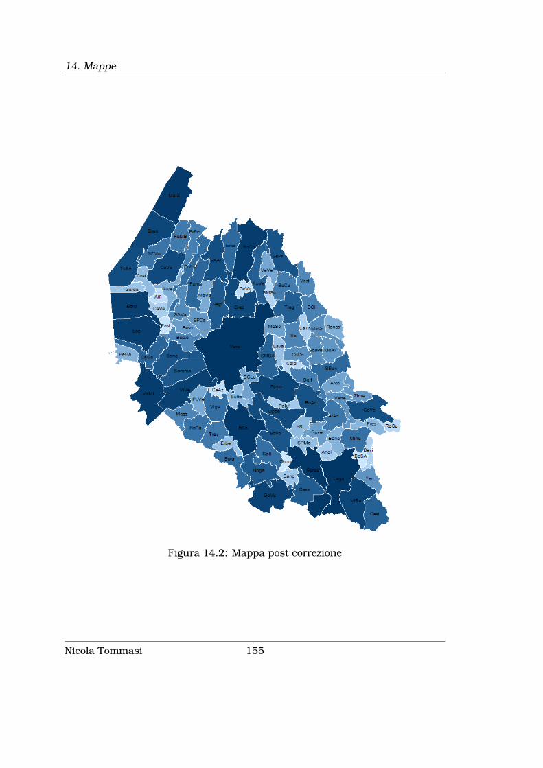
14. Mappe
Figura 14.2: Mappa post correzione
Nicola Tommasi 155
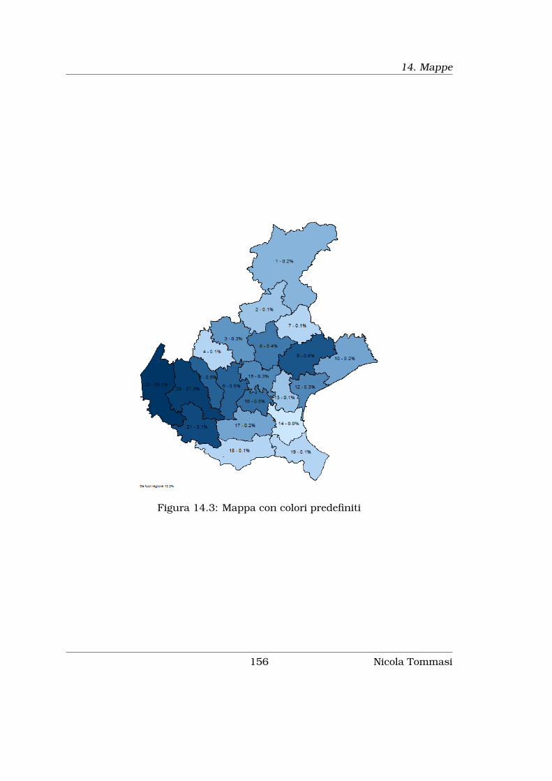
14. Mappe
Figura 14.3: Mappa con colori predefiniti
156 Nicola Tommasi

14. Mappe
------------+-----------------------------------0 | 1 4.55 4.551 | 4 18.18 22.732 | 2 9.09 31.823 | 1 4.55 36.364 | 2 9.09 45.455 | 1 4.55 50.006 | 2 9.09 59.097 | 1 4.55 63.649 | 1 4.55 68.1810 | 2 9.09 77.2711 | 1 4.55 81.8259 | 1 4.55 86.36234 | 1 4.55 90.91526 | 1 4.55 95.45
1022 | 1 4.55 100.00------------+-----------------------------------
Total | 22 100.00
. local colors = "";
. local rgb navy;
. local ncl = r(r) - 2;
. local INTY =0.75;
. local inty =0.01;
. local step = (`INTY'-`inty') / `ncl';
. local step = round(`step',0.01);
. forvalues c = 0(1)`ncl' ;local x = `inty' + `step'*`c';local x = round(`x',0.01);local colors = "`colors'" + "`rgb'*`x' ";
;. di "`colors'";navy*.01 navy*.07 navy*.13 navy*.19 navy*.25 navy*.31 navy*.37 navy*.43 navy*.49 navy*.55> navy*.61 navy*.67 navy*.73 navy*.79
. spmap pedia_odp using coord_ulss.dta, id(_ID) fcolor(white `colors') ocolor(black ..) clmethod(unique)> label(label(pedia_odpstr) x(x_c) y(y_c) size(1.8) length(14)) legenda(off) split> note("Da fuori regione `pedia_odpFP'%", size(*0.50));
. graph export graph/ric_tot/pedia_od1.png, replace;(file graph/ric_tot/pedia_od1.png written in PNG format)
e questo è il risultato:In particolare le aree con numrosità pari a zero saranno bianche fcolor(white..., mentre la successiva parte da un valore navy*.01, per passare ad unnavy*.07, quindi a un navy*.13 e così via.
Nicola Tommasi 157
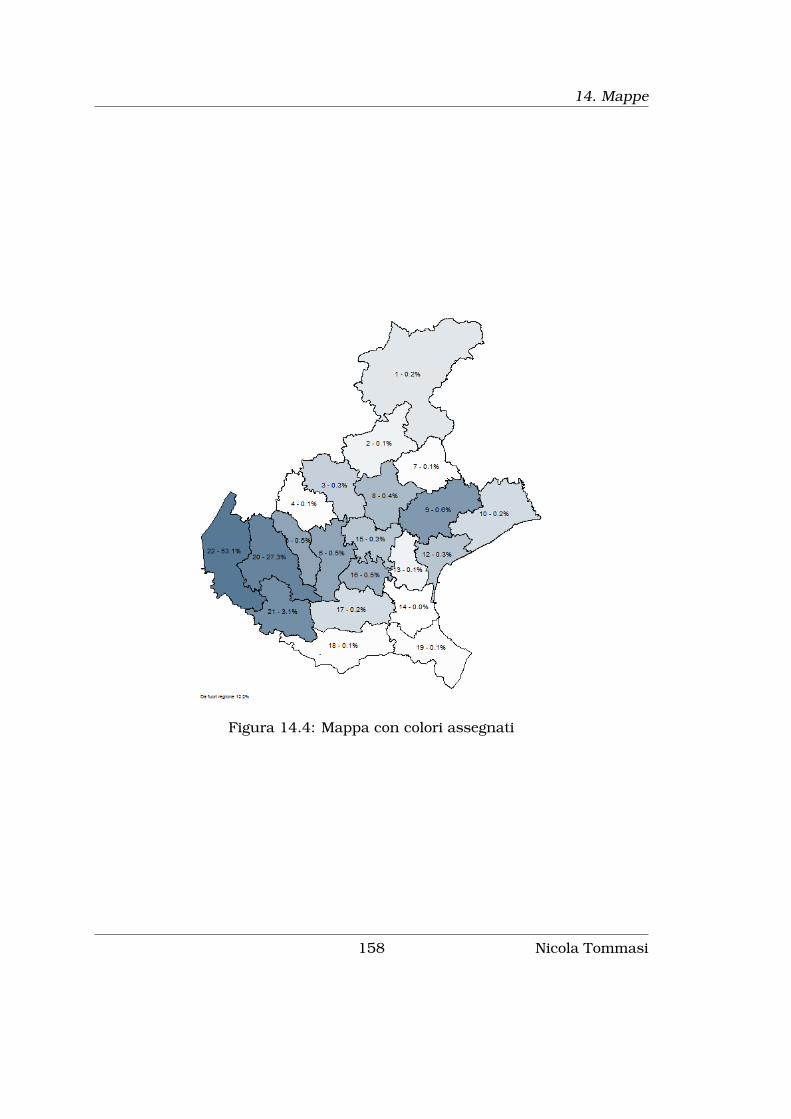
14. Mappe
Figura 14.4: Mappa con colori assegnati
158 Nicola Tommasi

Parte II
Casi Applicati
159

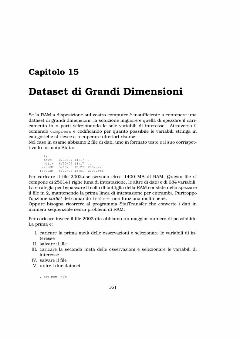
Capitolo 15
Dataset di Grandi Dimensioni
Se la RAM a disposizione sul vostro computer è insufficiente a contenere unadataset di grandi dimensioni, la soluzione migliore è quella di spezzare il cari-camento in n parti selezionando le sole variabili di interesse. Attraverso ilcomando compress e codificando per quanto possibile le variabili stringa incategoriche si riesce a recuperare ulteriori risorse.Nel caso in esame abbiamo 2 file di dati, uno in formato testo e il suo corrispet-tivo in formato Stata:
. ls<dir> 8/30/07 14:17 .<dir> 8/30/07 14:17 ..770.8M 5/15/06 12:27 2002.asc1370.2M 5/22/06 18:51 2002.dta
Per caricare il file 2002.asc servono circa 1400 MB di RAM. Questo file sicompone di 256141 righe (una di intestazione, le altre di dati) e di 684 variabili.La strategia per bypassare il collo di bottiglia della RAM consiste nello spezzareil file in 2, mantenendo la prima linea di intestazione per entrambi. Purtroppol’opzione varlist del comando insheet non funziona molto bene.Oppure bisogna ricorrere al programma StatTransfer che converte i dati inmaniera sequenziale senza problemi di RAM.
Per caricare invece il file 2002.dta abbiamo un maggior numero di possibilità.La prima è:
I. caricare la prima metà delle osservazioni e selezionare le variabili di in-teresse
II. salvare il fileIII. caricare la seconda metà delle osservazioni e selezionare le variabili di
interesseIV. salvare il fileV. unire i due dataset
. set mem 740m
161

15. Dataset di Grandi Dimensioni
Current memory allocation
current memory usagesettable value description (1M = 1024k)--------------------------------------------------------------------set maxvar 5000 max. variables allowed 1.909Mset memory 740M max. data space 740.000Mset matsize 400 max. RHS vars in models 1.254M
-----------743.163M
. use 2002.dta in 1/128070
. desc, short
Contains data from 2002.dtaobs: 128,070vars: 669 22 May 2006 18:49size: 718,856,910 (7.4% of memory free)Sorted by:
. keep h01 h03 h08 h12
. save tmp1, replace(note: file tmp1.dta not found)file tmp1.dta saved
. use 2002.dta in 128071/256140
. desc, short
Contains data from 2002.dtaobs: 128,070vars: 669 22 May 2006 18:49size: 718,856,910 (7.4% of memory free)Sorted by:
. keep h01 h03 h08 h12
. save tmp2, replace(note: file tmp2.dta not found)file tmp2.dta saved
. compressh08 was str40 now str33h12 was str15 now str14
. append using tmp1h08 was str33 now str40h12 was str14 now str15
. desc, short
Contains data from tmp2.dtaobs: 256,140vars: 4 30 Aug 2007 15:17size: 35,347,320 (95.4% of memory free)Sorted by:
Note: dataset has changed since last saved
La seconda strategia invece consiste nel leggere direttamente tutte le osser-vazioni per le sole variabili di interesse:
162 Nicola Tommasi

15. Dataset di Grandi Dimensioni
. set mem 740m
Current memory allocation
current memory usagesettable value description (1M = 1024k)--------------------------------------------------------------------set maxvar 5000 max. variables allowed 1.909Mset memory 740M max. data space 740.000Mset matsize 400 max. RHS vars in models 1.254M
-----------743.163M
. use h01 h03 h08 h12 using 2002.dta, clear
. desc, short
Contains data from 2002.dtaobs: 256,140vars: 4 22 May 2006 18:49size: 35,347,320 (95.4% of memory free)Sorted by:
Nicola Tommasi 163


Capitolo 16
Da Stringa a Numerica
16.1 Fondere variabili stringa con numeriche
Se ci si trova con due variabili che contengono la stessa informazione ma inuna espressa in forma numerica e nell’altra espressa come stringa, possiamoridurle in maniera semplice in una sola, utilizzando l’informazione della vari-abile stringa per costruire il label define per la variabile numerica. Se peresempio abbiamo due variabili con questi possibili valori:
cod_reg regione1 Piemonte2 Valle d’Aosta3 Lombardia4 Trentino-Alto Adige5 Veneto6 Friuli-Venezia Giulia7 Liguria8 Emilia-Romagna9 Toscana10 Umbria11 Marche12 Lazio13 Abruzzo14 Molise15 Campania16 Puglia17 Basilicata18 Calabria19 Sicilia20 Sardegna
165

16.1. Fondere variabili stringa con numeriche 16. Da Stringa a Numerica
e vogliamo assegnare come label dei valori di cod_reg la descrizione contenutanella variabile regione, possiamo, in maniera pedante, fare:
label define cod_reg 1 "Piemonte"2 "Valle d´Aosta".....20 "Sardegna";
label values cod_reg cod_reg;
oppure installare il comando labutil
ssc inst labutil
e poi
. tab1 regione cod_reg
-> tabulation of regione
regione | Freq. Percent Cum.----------------------+-----------------------------------
Abruzzo | 61,610 3.76 3.76Basilicata | 26,462 1.62 5.38Calabria | 82,618 5.05 10.43Campania | 111,302 6.80 17.23
Emilia-Romagna | 68,882 4.21 21.44Friuli-Venezia Giulia | 44,238 2.70 24.14
Lazio | 76,356 4.66 28.80Liguria | 47,470 2.90 31.70
Lombardia | 312,696 19.10 50.81Marche | 49,692 3.04 53.84Molise | 27,472 1.68 55.52
Piemonte | 243,612 14.88 70.41Puglia | 52,116 3.18 73.59
Sardegna | 76,154 4.65 78.24Sicilia | 78,780 4.81 83.06Toscana | 57,974 3.54 86.60
Trentino-Alto Adige | 68,478 4.18 90.78Umbria | 18,584 1.14 91.92
Valle d´Aosta | 14,948 0.91 92.83Veneto | 117,362 7.17 100.00
----------------------+-----------------------------------Total | 1,636,806 100.00
-> tabulation of cod_reg
cod_reg | Freq. Percent Cum.------------+-----------------------------------
1 | 243,612 14.88 14.882 | 14,948 0.91 15.803 | 312,696 19.10 34.904 | 68,478 4.18 39.085 | 117,362 7.17 46.256 | 44,238 2.70 48.967 | 47,470 2.90 51.868 | 68,882 4.21 56.079 | 57,974 3.54 59.6110 | 18,584 1.14 60.7411 | 49,692 3.04 63.7812 | 76,356 4.66 68.4413 | 61,610 3.76 72.2114 | 27,472 1.68 73.8915 | 111,302 6.80 80.6916 | 52,116 3.18 83.87
166 Nicola Tommasi
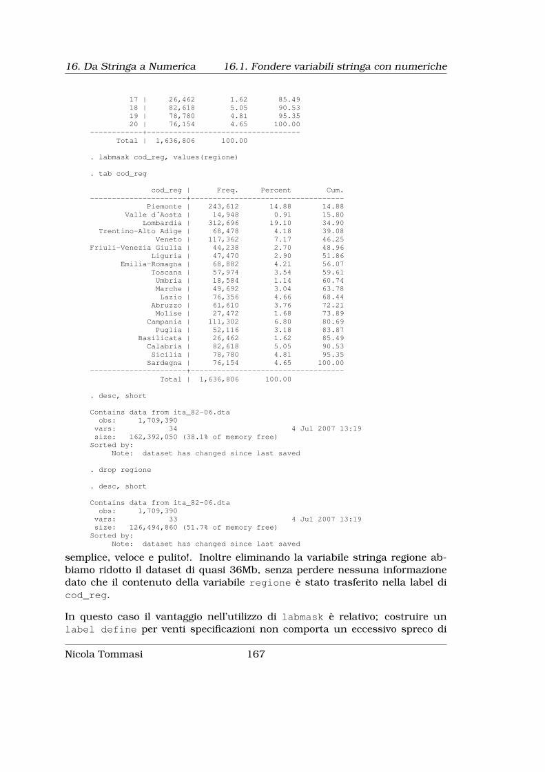
16. Da Stringa a Numerica 16.1. Fondere variabili stringa con numeriche
17 | 26,462 1.62 85.4918 | 82,618 5.05 90.5319 | 78,780 4.81 95.3520 | 76,154 4.65 100.00
------------+-----------------------------------Total | 1,636,806 100.00
. labmask cod_reg, values(regione)
. tab cod_reg
cod_reg | Freq. Percent Cum.----------------------+-----------------------------------
Piemonte | 243,612 14.88 14.88Valle d´Aosta | 14,948 0.91 15.80
Lombardia | 312,696 19.10 34.90Trentino-Alto Adige | 68,478 4.18 39.08
Veneto | 117,362 7.17 46.25Friuli-Venezia Giulia | 44,238 2.70 48.96
Liguria | 47,470 2.90 51.86Emilia-Romagna | 68,882 4.21 56.07
Toscana | 57,974 3.54 59.61Umbria | 18,584 1.14 60.74Marche | 49,692 3.04 63.78Lazio | 76,356 4.66 68.44
Abruzzo | 61,610 3.76 72.21Molise | 27,472 1.68 73.89
Campania | 111,302 6.80 80.69Puglia | 52,116 3.18 83.87
Basilicata | 26,462 1.62 85.49Calabria | 82,618 5.05 90.53Sicilia | 78,780 4.81 95.35Sardegna | 76,154 4.65 100.00
----------------------+-----------------------------------Total | 1,636,806 100.00
. desc, short
Contains data from ita_82-06.dtaobs: 1,709,390vars: 34 4 Jul 2007 13:19size: 162,392,050 (38.1% of memory free)Sorted by:
Note: dataset has changed since last saved
. drop regione
. desc, short
Contains data from ita_82-06.dtaobs: 1,709,390vars: 33 4 Jul 2007 13:19size: 126,494,860 (51.7% of memory free)Sorted by:
Note: dataset has changed since last saved
semplice, veloce e pulito!. Inoltre eliminando la variabile stringa regione ab-biamo ridotto il dataset di quasi 36Mb, senza perdere nessuna informazionedato che il contenuto della variabile regione è stato trasferito nella label dicod_reg.
In questo caso il vantaggio nell’utilizzo di labmask è relativo; costruire unlabel define per venti specificazioni non comporta un eccessivo spreco di
Nicola Tommasi 167

16.2. Da stringa a numerica categorica 16. Da Stringa a Numerica
tempo, ma pensate se dovete fare la stessa cosa per il label delle provincie ital-iane (più di cento) o dei comuni italiani che sono più di ottomila!!! (io l’ho fattoe ottomila comuni sono tanti).
16.2 Da stringa a numerica categorica
Supponiamo di avere una variabile stringa (basale) che assume le seguentispecificazioni:
NO SHUNT<10>10 SINGLE SPIKES>10 SHOWER O CURTAIN
e che vogliamo trasformarla in una variabile numerica categorica con questeassegnazioni:
0 per "NO SHUNT"1 per "<10"2 per ">10 SINGLE SPIKES"3 per ">10 SHOWER O CURTAIN"
Invece di ricorrere alla costruzione
replace basale="0" if basale=="NO SHUNT";replace basale="1" if basale=="<10";replace basale="2" if basale==">10 SINGLE SPIKES";replace basale="3" if basale==">10 SHOWER O CURTAIN";destring basale valsalva, replace;label define shunt 0 "no shunt"
1 "<10"2 ">10 SINGLE SPIKES"3 ">10 SHOWER O CURTAIN";
label values basale shunt;
possiamo fare:
label define shunt 0 "no shunt"1 "<10"2 ">10 SINGLE SPIKES"3 ">10 SHOWER O CURTAIN";
encode basale, gen(basale_n) label(shunt);
dove in gen() si mette la nuova variabile numerica che verrà creata e i cui val-ori corrispondono a quelli definiti in label define. Notare che è obbligatoriocreare una nuova variabile perché al momento il comando encode non prevedel’opzione replace.
168 Nicola Tommasi

Capitolo 17
Liste di Files e Directory
Il problema da risolvere è l’acquisizione e la riunione in un unico dataset delleinformazioni contenute in un elevato numero di files. In questo caso abbiamole venti regioni italiane
. dir, wide<dir> . <dir> .. <dir> abruzzo<dir> basilicata <dir> calabria <dir> campania<dir> emilia_romagna <dir> friuli <dir> lazio<dir> liguria <dir> lombardia <dir> marche<dir> molise <dir> piemonte <dir> puglia<dir> sardegna <dir> sicilia <dir> toscana<dir> trentino <dir> umbria <dir> vda<dir> veneto
All’interno di ciascuna regione abbiamo un cartella per ciascuna provincia diquella regione:
. cd abruzzoG:\projects\popolazione\pop_res\com_82-01\abruzzo
. dir<dir> 7/04/07 10:36 .<dir> 7/04/07 10:36 ..<dir> 7/04/07 10:35 chieti<dir> 7/04/07 10:36 laquila<dir> 7/04/07 10:36 pescara<dir> 7/04/07 10:36 teramo
All’interno di ciascuna cartella delle provincie, una cartella dati che contiene2 tipi di dati:
- una serie di files con estensione .TXT, con dati in formato testo delimitatida virgola. Per ogni comune della provincia c’è un file che contiene idati inerenti alle femmine (*_F.TXT) e un file con i dati inerenti i maschi(*_M.TXT).
- una serie di files con estensione .csv, con dati in formato testo delimitatida virgola. In questo caso c’è un unico file per ciascun anno dal dal 1992al 2001 con i dati sia dei maschi che delle femmine.
169

17. Liste di Files e Directory
. cd chieti/datiG:\projects\popolazione\pop_res\com_82-01\abruzzo\chieti\dati
. dir, wide<dir> . <dir> .. 4.2k 069001_F.TXT4.2k 069001_M.TXT 4.2k 069002_F.TXT 4.2k 069002_M.TXT3.8k 069003_F.TXT 3.8k 069003_M.TXT 3.7k 069004_F.TXT3.7k 069004_M.TXT 4.3k 069005_F.TXT 4.3k 069005_M.TXT3.7k 069006_F.TXT 3.6k 069006_M.TXT 3.5k 069007_F.TXT3.5k 069007_M.TXT 4.3k 069008_F.TXT 4.3k 069008_M.TXT3.5k 069009_F.TXT 3.5k 069009_M.TXT 3.8k 069010_F.TXT3.8k 069010_M.TXT 3.5k 069011_F.TXT 3.5k 069011_M.TXT3.6k 069012_F.TXT 3.6k 069012_M.TXT 3.8k 069013_F.TXT3.7k 069013_M.TXT 3.7k 069014_F.TXT 3.7k 069014_M.TXT4.3k 069015_F.TXT 4.3k 069015_M.TXT 4.2k 069016_F.TXT4.2k 069016_M.TXT 4.3k 069017_F.TXT 4.3k 069017_M.TXT4.3k 069018_F.TXT 4.3k 069018_M.TXT 3.5k 069019_F.TXT3.5k 069019_M.TXT 4.2k 069020_F.TXT 4.2k 069020_M.TXT3.7k 069021_F.TXT 3.7k 069021_M.TXT 5.2k 069022_F.TXT5.1k 069022_M.TXT 3.5k 069023_F.TXT 3.5k 069023_M.TXT3.7k 069024_F.TXT 3.6k 069024_M.TXT 3.5k 069025_F.TXT3.5k 069025_M.TXT 3.5k 069026_F.TXT 3.5k 069026_M.TXT4.3k 069027_F.TXT 4.3k 069027_M.TXT 4.3k 069028_F.TXT4.3k 069028_M.TXT 3.5k 069029_F.TXT 3.5k 069029_M.TXT4.0k 069030_F.TXT 3.9k 069030_M.TXT 4.0k 069031_F.TXT3.9k 069031_M.TXT 3.7k 069032_F.TXT 3.6k 069032_M.TXT4.3k 069033_F.TXT 4.3k 069033_M.TXT 3.5k 069034_F.TXT3.5k 069034_M.TXT 4.9k 069035_F.TXT 4.9k 069035_M.TXT3.7k 069036_F.TXT 3.7k 069036_M.TXT 4.1k 069037_F.TXT4.0k 069037_M.TXT 3.8k 069038_F.TXT 3.8k 069038_M.TXT3.5k 069039_F.TXT 3.5k 069039_M.TXT 4.0k 069040_F.TXT4.0k 069040_M.TXT 4.3k 069041_F.TXT 4.3k 069041_M.TXT3.7k 069042_F.TXT 3.7k 069042_M.TXT 4.3k 069043_F.TXT4.3k 069043_M.TXT 3.5k 069044_F.TXT 3.5k 069044_M.TXT3.8k 069045_F.TXT 3.8k 069045_M.TXT 5.1k 069046_F.TXT5.1k 069046_M.TXT 3.5k 069047_F.TXT 3.5k 069047_M.TXT3.5k 069048_F.TXT 3.5k 069048_M.TXT 3.6k 069049_F.TXT3.6k 069049_M.TXT 4.3k 069050_F.TXT 4.3k 069050_M.TXT3.7k 069051_F.TXT 3.7k 069051_M.TXT 3.5k 069052_F.TXT3.5k 069052_M.TXT 3.5k 069053_F.TXT 3.5k 069053_M.TXT3.6k 069054_F.TXT 3.6k 069054_M.TXT 4.1k 069055_F.TXT4.1k 069055_M.TXT 4.0k 069056_F.TXT 4.0k 069056_M.TXT4.3k 069057_F.TXT 4.3k 069057_M.TXT 5.1k 069058_F.TXT5.0k 069058_M.TXT 4.3k 069059_F.TXT 4.3k 069059_M.TXT3.9k 069060_F.TXT 3.8k 069060_M.TXT 3.8k 069061_F.TXT3.8k 069061_M.TXT 3.7k 069062_F.TXT 3.7k 069062_M.TXT3.5k 069063_F.TXT 3.5k 069063_M.TXT 3.5k 069064_F.TXT3.5k 069064_M.TXT 3.9k 069065_F.TXT 3.9k 069065_M.TXT3.8k 069066_F.TXT 3.7k 069066_M.TXT 3.6k 069067_F.TXT3.6k 069067_M.TXT 4.2k 069068_F.TXT 4.2k 069068_M.TXT3.7k 069069_F.TXT 3.6k 069069_M.TXT 3.6k 069070_F.TXT3.6k 069070_M.TXT 3.9k 069071_F.TXT 3.9k 069071_M.TXT4.3k 069072_F.TXT 4.3k 069072_M.TXT 4.0k 069073_F.TXT4.0k 069073_M.TXT 4.2k 069074_F.TXT 4.2k 069074_M.TXT3.9k 069075_F.TXT 3.8k 069075_M.TXT 4.1k 069076_F.TXT4.1k 069076_M.TXT 3.5k 069077_F.TXT 3.5k 069077_M.TXT3.5k 069078_F.TXT 3.5k 069078_M.TXT 3.8k 069079_F.TXT3.7k 069079_M.TXT 3.5k 069080_F.TXT 3.5k 069080_M.TXT4.3k 069081_F.TXT 4.3k 069081_M.TXT 3.6k 069082_F.TXT3.5k 069082_M.TXT 4.7k 069083_F.TXT 4.7k 069083_M.TXT3.7k 069084_F.TXT 3.7k 069084_M.TXT 4.2k 069085_F.TXT4.2k 069085_M.TXT 4.3k 069086_F.TXT 4.3k 069086_M.TXT4.3k 069087_F.TXT 4.3k 069087_M.TXT 4.1k 069088_F.TXT4.0k 069088_M.TXT 3.5k 069089_F.TXT 3.5k 069089_M.TXT4.3k 069090_F.TXT 4.3k 069090_M.TXT 4.3k 069091_F.TXT
170 Nicola Tommasi

17. Liste di Files e Directory
4.3k 069091_M.TXT 4.1k 069092_F.TXT 4.0k 069092_M.TXT3.8k 069093_F.TXT 3.8k 069093_M.TXT 4.2k 069094_F.TXT4.2k 069094_M.TXT 4.0k 069095_F.TXT 3.9k 069095_M.TXT3.6k 069096_F.TXT 3.5k 069096_M.TXT 3.5k 069097_F.TXT3.5k 069097_M.TXT 3.9k 069098_F.TXT 3.9k 069098_M.TXT5.1k 069099_F.TXT 5.0k 069099_M.TXT 3.6k 069100_F.TXT3.6k 069100_M.TXT 4.2k 069101_F.TXT 4.1k 069101_M.TXT3.9k 069102_F.TXT 3.8k 069102_M.TXT 3.5k 069103_F.TXT3.5k 069103_M.TXT 3.5k 069104_F.TXT 3.5k 069104_M.TXT59.2k ch1992.csv 59.2k ch1993.csv 59.2k ch1994.csv59.2k ch1995.csv 59.2k ch1996.csv 59.2k ch1997.csv59.1k ch1998.csv 59.1k ch1999.csv 59.1k ch2000.csv59.0k ch2001.csv
per un totale di 16172 files .TXT e 1030 files .csv. Usare il comando insheetscrivendo il nome di tutti i files .TXT e .csv è la soluzione adottata da chidispone di molto tempo ed è veloce nella digitazione. Io che non ho il primo esono scarso nella seconda preferisco agire così.Per prima cosa acquisisco all’interno di una local i nomi di tutti i files informato .TXT:
. local files: dir . files "*.txt"
. di `"`files'"'"069001_f.txt" "069001_m.txt" "069002_f.txt" "069002_m.txt" "069003_f.txt" "0690> 03_m.txt" "069004_f.txt" "069004_m.txt" "069005_f.txt" "069005_m.txt" "069006_> f.txt" "069006_m.txt" "069007_f.txt" "069007_m.txt" "069008_f.txt" "069008_m.t> xt" "069009_f.txt" "069009_m.txt" "069010_f.txt" "069010_m.txt" "069011_f.txt"> "069011_m.txt" "069012_f.txt" "069012_m.txt" "069013_f.txt" "069013_m.txt" "0> 69014_f.txt" "069014_m.txt" "069015_f.txt" "069015_m.txt" "069016_f.txt" "0690> 16_m.txt" "069017_f.txt" "069017_m.txt" "069018_f.txt" "069018_m.txt" "069019_> f.txt" "069019_m.txt" "069020_f.txt" "069020_m.txt" "069021_f.txt" "069021_m.t> xt" "069022_f.txt" "069022_m.txt" "069023_f.txt" "069023_m.txt" "069024_f.txt"> "069024_m.txt" "069025_f.txt" "069025_m.txt" "069026_f.txt" "069026_m.txt" "0> 69027_f.txt" "069027_m.txt" "069028_f.txt" "069028_m.txt" "069029_f.txt" "0690> 29_m.txt" "069030_f.txt" "069030_m.txt" "069031_f.txt" "069031_m.txt" "069032_> f.txt" "069032_m.txt" "069033_f.txt" "069033_m.txt" "069034_f.txt" "069034_m.t> xt" "069035_f.txt" "069035_m.txt" "069036_f.txt" "069036_m.txt" "069037_f.txt"> "069037_m.txt" "069038_f.txt" "069038_m.txt" "069039_f.txt" "069039_m.txt" "0> 69040_f.txt" "069040_m.txt" "069041_f.txt" "069041_m.txt" "069042_f.txt" "0690> 42_m.txt" "069043_f.txt" "069043_m.txt" "069044_f.txt" "069044_m.txt" "069045_> f.txt" "069045_m.txt" "069046_f.txt" "069046_m.txt" "069047_f.txt" "069047_m.t> xt" "069048_f.txt" "069048_m.txt" "069049_f.txt" "069049_m.txt" "069050_f.txt"> "069050_m.txt" "069051_f.txt" "069051_m.txt" "069052_f.txt" "069052_m.txt" "0> 69053_f.txt" "069053_m.txt" "069054_f.txt" "069054_m.txt" "069055_f.txt" "0690> 55_m.txt" "069056_f.txt" "069056_m.txt" "069057_f.txt" "069057_m.txt" "069058_> f.txt" "069058_m.txt" "069059_f.txt" "069059_m.txt" "069060_f.txt" "069060_m.t> xt" "069061_f.txt" "069061_m.txt" "069062_f.txt" "069062_m.txt" "069063_f.txt"> "069063_m.txt" "069064_f.txt" "069064_m.txt" "069065_f.txt" "069065_m.txt" "0> 69066_f.txt" "069066_m.txt" "069067_f.txt" "069067_m.txt" "069068_f.txt" "0690> 68_m.txt" "069069_f.txt" "069069_m.txt" "069070_f.txt" "069070_m.txt" "069071_> f.txt" "069071_m.txt" "069072_f.txt" "069072_m.txt" "069073_f.txt" "069073_m.t> xt" "069074_f.txt" "069074_m.txt" "069075_f.txt" "069075_m.txt" "069076_f.txt"> "069076_m.txt" "069077_f.txt" "069077_m.txt" "069078_f.txt" "069078_m.txt" "0> 69079_f.txt" "069079_m.txt" "069080_f.txt" "069080_m.txt" "069081_f.txt" "0690> 81_m.txt" "069082_f.txt" "069082_m.txt" "069083_f.txt" "069083_m.txt" "069084_> f.txt" "069084_m.txt" "069085_f.txt" "069085_m.txt" "069086_f.txt" "069086_m.t> xt" "069087_f.txt" "069087_m.txt" "069088_f.txt" "069088_m.txt" "069089_f.txt"> "069089_m.txt" "069090_f.txt" "069090_m.txt" "069091_f.txt" "069091_m.txt" "0> 69092_f.txt" "069092_m.txt" "069093_f.txt" "069093_m.txt" "069094_f.txt" "0690> 94_m.txt" "069095_f.txt" "069095_m.txt" "069096_f.txt" "069096_m.txt" "069097_> f.txt" "069097_m.txt" "069098_f.txt" "069098_m.txt" "069099_f.txt" "069099_m.t
Nicola Tommasi 171

17. Liste di Files e Directory
> xt" "069100_f.txt" "069100_m.txt" "069101_f.txt" "069101_m.txt" "069102_f.txt"> "069102_m.txt" "069103_f.txt" "069103_m.txt" "069104_f.txt" "069104_m.txt"
La costruzione local files: dir . files *.txt rientra nelle funzioniestese delle macro di Stata ([P] macro)1.A questo punto per poter fare l’append dei dati devo partire con il primo file,salvarlo e poi fare l’append dei successivi file. Per fare ciò, estraggo dalla localche ho chiamato files il suo primo elemento, lo assegno alla local che chi-amerò primo e contestualmente lo tolgo dalla local files per non leggeredue volte lo stesso file di dati `'
. local primo : word 1 of `files' /* primo elemento di `files' */
. di "`primo'"069001_f.txt
. local files : list files - primo /* tolgo da `files' il suo primo elemento */
Anche la costruzione local primo : word 1 of `files' appartiene allefunzioni estese delle macro di Stata. A questo punto leggo i dati del primo file(quello indicato dalla local primo), genero la variabile sex, le assegno valore2 e lo salvo in un file temporaneo:
. insheet using `primo', clear(14 vars, 87 obs)
. gen sex=2
. save temp, replace(note: file temp.dta not found)file temp.dta saved
Ora posso leggere e fare l’append in sequenza di tutti gli altri file indicati nellalocal files. Devo però distinguere i files con dati riferiti alle femmine daifiles con dati riferiti ai maschi. Come? Se nel nome del file c’è _m sarannodati riferiti a maschi e quindi assegnerò valore uno alla variabile sex, se c'è _fsaranno dati riferiti alle femmine e quindi assegnerò valore due alla variabilesex. La costruzione local meccia = strmatch(`f',*_m*) mi permette didistinguere tra le 2 possibilità e quindi di agire di conseguenza sul valore daassegnare alla variabile sex.
foreach f in `files' {;insheet using dati/`f', clear;local meccia = strmatch("`f'","*_m*");if `meccia'==1 {; /* se trova _m nel nome del file */
gen sex=1; /* assegna a sex il valore 1 */};else if `meccia'==0 {; /* altrimenti */
gen sex=2; /* assegna a sex il valore 2 */};
append using temp;save temp, replace;
};
1Notare la particolare sintassi usata per fare il display della local files!!
172 Nicola Tommasi

17. Liste di Files e Directory
. summ
Variable | Obs Mean Std. Dev. Min Max-------------+--------------------------------------------------------
v1 | 0v2 | 18096 69052.5 30.02166 69001 69104v3 | 0v4 | 18096 43.14943 25.40616 0 99v5 | 18096 40.94828 437.5124 0 29005
-------------+--------------------------------------------------------v6 | 18096 41.16534 441.2414 0 29067v7 | 18096 41.30836 444.0427 0 29125v8 | 18096 41.46795 446.7315 0 29183v9 | 18096 41.58709 449.089 0 29241v10 | 18096 41.66225 450.6736 0 29273
-------------+--------------------------------------------------------v11 | 18096 41.75696 452.6105 0 29311v12 | 18096 41.91943 455.5657 0 29404v13 | 18096 42.05449 458.2125 0 29479v14 | 18096 42.1408 460.1403 0 29603sex | 18096 1.5 .5000138 1 2
Bene, risolto il problema dei files; ma vorrei potermi muovere anche tra leventi cartelle delle regioni e tra le cartelle delle provincie sfruttando lo stessomeccanismo. No problem, basta sfruttare la funzione dir . dirs:
. local regioni : dir . dirs "*";
. di `"`regioni'"';"abruzzo" "basilicata" "calabria" "campania" "emilia_romagna" "friuli" "lazio""liguria" "lombardia" "marche" "molise" "piemonte" "puglia" "sardegna" "sicilia""toscana" "trentino" "umbria" "vda" "veneto"
Adesso facciamo in modo di entrare in ciascuna cartella delle regione e lanciareil file prov.do in questo modo:
foreach regio in `regioni' {;cd `regio';do prov.do;cd ..;};
Il file prov.do a sua volta raccoglie l’elenco delle cartelle delle provincie e lanciail file read.do che si occupa di leggere i dati dai files .TXT e .csv.
local diry : dir . dirs "*";di `"`diry'"';"chieti" "laquila" "pescara" "teramo"
foreach prv in `diry' {;cd `prv';do read.do;cd ..;};
Nicola Tommasi 173


Capitolo 18
Previsioni Multiple
18.1 Introduzione
Spiego brevemente il contesto e il problema che si vuole risolvere. Si vuolestimare attraverso un modello probit la probabilità di separazione di un grup-po di coppie in base ad un ridotto numero di variabili esplicative. In realtàle variabili esplicative sarebbero molto più numerose ma in questo esempioutilizziamo solo quelle necessarie per produrre un insieme di probabilità diseparazione data da tutte le possibili combinazioni delle variabili esplicative.Per fare ciò ricorreremo al comando contract, ad un ciclo foreach, a matricie al comando aggiuntivo prchange implementato da J. Scott Long e JeremyFreese.
18.2 La stima del modello
Come già detto stimiamo un versione ridotta del modello. Vediamo una de-scrizione delle variabili utilizzate e il risultato della stima probit:
. summ separazione higher_edu_M_l higher_edu_F_l> du_dip_M du_self_M du_nw_F du_dip_F;
Variable | Obs Mean Std. Dev. Min Max-------------+--------------------------------------------------------separazione | 4865 .0341213 .1815593 0 1higher_e~M_l | 4810 .1039501 .3052275 0 1higher_e~F_l | 4830 .0917184 .2886579 0 1
du_dip_M | 4845 .580805 .4934783 0 1du_self_M | 4845 .2637771 .4407253 0 1
-------------+--------------------------------------------------------du_nw_F | 4859 .5330315 .4989591 0 1du_dip_F | 4859 .370035 .4828634 0 1
. probit separazione sons_M_l higher_edu_M_l higher_edu_F_l du_dip_M> du_self_M du_nw_F du_dip_F;
Iteration 0: log likelihood = -721.19595Iteration 1: log likelihood = -702.70504
175
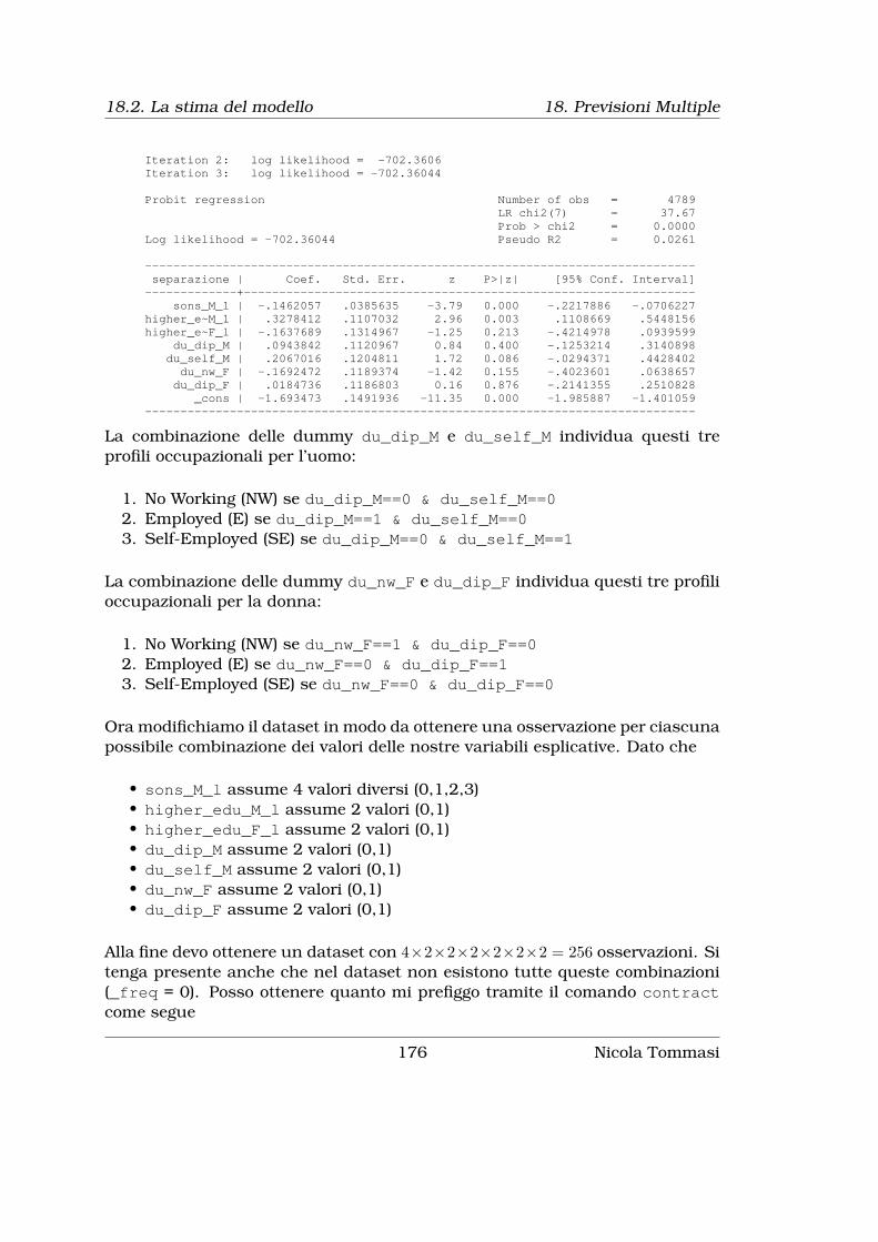
18.2. La stima del modello 18. Previsioni Multiple
Iteration 2: log likelihood = -702.3606Iteration 3: log likelihood = -702.36044
Probit regression Number of obs = 4789LR chi2(7) = 37.67Prob > chi2 = 0.0000
Log likelihood = -702.36044 Pseudo R2 = 0.0261
------------------------------------------------------------------------------separazione | Coef. Std. Err. z P>|z| [95% Conf. Interval]-------------+----------------------------------------------------------------
sons_M_l | -.1462057 .0385635 -3.79 0.000 -.2217886 -.0706227higher_e~M_l | .3278412 .1107032 2.96 0.003 .1108669 .5448156higher_e~F_l | -.1637689 .1314967 -1.25 0.213 -.4214978 .0939599
du_dip_M | .0943842 .1120967 0.84 0.400 -.1253214 .3140898du_self_M | .2067016 .1204811 1.72 0.086 -.0294371 .4428402
du_nw_F | -.1692472 .1189374 -1.42 0.155 -.4023601 .0638657du_dip_F | .0184736 .1186803 0.16 0.876 -.2141355 .2510828
_cons | -1.693473 .1491936 -11.35 0.000 -1.985887 -1.401059------------------------------------------------------------------------------
La combinazione delle dummy du_dip_M e du_self_M individua questi treprofili occupazionali per l’uomo:
1. No Working (NW) se du_dip_M==0 & du_self_M==02. Employed (E) se du_dip_M==1 & du_self_M==03. Self-Employed (SE) se du_dip_M==0 & du_self_M==1
La combinazione delle dummy du_nw_F e du_dip_F individua questi tre profilioccupazionali per la donna:
1. No Working (NW) se du_nw_F==1 & du_dip_F==02. Employed (E) se du_nw_F==0 & du_dip_F==13. Self-Employed (SE) se du_nw_F==0 & du_dip_F==0
Ora modifichiamo il dataset in modo da ottenere una osservazione per ciascunapossibile combinazione dei valori delle nostre variabili esplicative. Dato che
• sons_M_l assume 4 valori diversi (0,1,2,3)• higher_edu_M_l assume 2 valori (0,1)• higher_edu_F_l assume 2 valori (0,1)• du_dip_M assume 2 valori (0,1)• du_self_M assume 2 valori (0,1)• du_nw_F assume 2 valori (0,1)• du_dip_F assume 2 valori (0,1)
Alla fine devo ottenere un dataset con 4×2×2×2×2×2×2 = 256 osservazioni. Sitenga presente anche che nel dataset non esistono tutte queste combinazioni(_freq = 0). Posso ottenere quanto mi prefiggo tramite il comando contractcome segue
176 Nicola Tommasi

18. Previsioni Multiple 18.2. La stima del modello
. contract sons_M_l higher_edu_M_l higher_edu_F_l du_dip_M> du_self_M du_nw_F du_dip_F, nomiss zero;
. clist
sons_M_l highe~M_l highe~F_l du_dip_M du_sel~M du_dip_F du_nw_F _freq1. 0 0 0 0 0 0 0 82. 0 0 0 0 0 1 0 263. 0 0 0 0 0 0 1 1054. 0 0 0 0 0 1 1 05. 0 0 0 0 1 0 0 396. 0 0 0 0 1 1 0 777. 0 0 0 0 1 0 1 608. 0 0 0 0 1 1 1 09. 0 0 0 1 0 0 0 3110. 0 0 0 1 0 1 0 22211. 0 0 0 1 0 0 1 16212. 0 0 0 1 0 1 1 013. 0 0 0 1 1 0 0 014. 0 0 0 1 1 1 0 015. 0 0 0 1 1 0 1 016. 0 0 0 1 1 1 1 017. 0 0 1 0 0 0 0 118. 0 0 1 0 0 1 0 119. 0 0 1 0 0 0 1 020. 0 0 1 0 0 1 1 021. 0 0 1 0 1 0 0 722. 0 0 1 0 1 1 0 723. 0 0 1 0 1 0 1 324. 0 0 1 0 1 1 1 025. 0 0 1 1 0 0 0 426. 0 0 1 1 0 1 0 2227. 0 0 1 1 0 0 1 1028. 0 0 1 1 0 1 1 029. 0 0 1 1 1 0 0 030. 0 0 1 1 1 1 0 031. 0 0 1 1 1 0 1 032. 0 0 1 1 1 1 1 033. 0 1 0 0 0 0 0 134. 0 1 0 0 0 1 0 235. 0 1 0 0 0 0 1 136. 0 1 0 0 0 1 1 037. 0 1 0 0 1 0 0 438. 0 1 0 0 1 1 0 339. 0 1 0 0 1 0 1 840. 0 1 0 0 1 1 1 041. 0 1 0 1 0 0 0 242. 0 1 0 1 0 1 0 1543. 0 1 0 1 0 0 1 844. 0 1 0 1 0 1 1 045. 0 1 0 1 1 0 0 046. 0 1 0 1 1 1 0 047. 0 1 0 1 1 0 1 048. 0 1 0 1 1 1 1 049. 0 1 1 0 0 0 0 050. 0 1 1 0 0 1 0 051. 0 1 1 0 0 0 1 052. 0 1 1 0 0 1 1 053. 0 1 1 0 1 0 0 154. 0 1 1 0 1 1 0 855. 0 1 1 0 1 0 1 156. 0 1 1 0 1 1 1 057. 0 1 1 1 0 0 0 658. 0 1 1 1 0 1 0 1359. 0 1 1 1 0 0 1 8
Nicola Tommasi 177

18.2. La stima del modello 18. Previsioni Multiple
60. 0 1 1 1 0 1 1 061. 0 1 1 1 1 0 0 062. 0 1 1 1 1 1 0 063. 0 1 1 1 1 0 1 064. 0 1 1 1 1 1 1 065. 1 0 0 0 0 0 0 2066. 1 0 0 0 0 1 0 5767. 1 0 0 0 0 0 1 18068. 1 0 0 0 0 1 1 069. 1 0 0 0 1 0 0 7370. 1 0 0 0 1 1 0 8971. 1 0 0 0 1 0 1 16772. 1 0 0 0 1 1 1 073. 1 0 0 1 0 0 0 3374. 1 0 0 1 0 1 0 33575. 1 0 0 1 0 0 1 40576. 1 0 0 1 0 1 1 077. 1 0 0 1 1 0 0 078. 1 0 0 1 1 1 0 079. 1 0 0 1 1 0 1 080. 1 0 0 1 1 1 1 081. 1 0 1 0 0 0 0 082. 1 0 1 0 0 1 0 183. 1 0 1 0 0 0 1 384. 1 0 1 0 0 1 1 085. 1 0 1 0 1 0 0 686. 1 0 1 0 1 1 0 1287. 1 0 1 0 1 0 1 788. 1 0 1 0 1 1 1 089. 1 0 1 1 0 0 0 290. 1 0 1 1 0 1 0 3391. 1 0 1 1 0 0 1 1092. 1 0 1 1 0 1 1 093. 1 0 1 1 1 0 0 094. 1 0 1 1 1 1 0 095. 1 0 1 1 1 0 1 096. 1 0 1 1 1 1 1 097. 1 1 0 0 0 0 0 098. 1 1 0 0 0 1 0 199. 1 1 0 0 0 0 1 0100. 1 1 0 0 0 1 1 0101. 1 1 0 0 1 0 0 3102. 1 1 0 0 1 1 0 14103. 1 1 0 0 1 0 1 11104. 1 1 0 0 1 1 1 0105. 1 1 0 1 0 0 0 4106. 1 1 0 1 0 1 0 31107. 1 1 0 1 0 0 1 20108. 1 1 0 1 0 1 1 0109. 1 1 0 1 1 0 0 0110. 1 1 0 1 1 1 0 0111. 1 1 0 1 1 0 1 0112. 1 1 0 1 1 1 1 0113. 1 1 1 0 0 0 0 1114. 1 1 1 0 0 1 0 0115. 1 1 1 0 0 0 1 1116. 1 1 1 0 0 1 1 0117. 1 1 1 0 1 0 0 6118. 1 1 1 0 1 1 0 9119. 1 1 1 0 1 0 1 8120. 1 1 1 0 1 1 1 0121. 1 1 1 1 0 0 0 4122. 1 1 1 1 0 1 0 40123. 1 1 1 1 0 0 1 17124. 1 1 1 1 0 1 1 0
178 Nicola Tommasi

18. Previsioni Multiple 18.2. La stima del modello
125. 1 1 1 1 1 0 0 0126. 1 1 1 1 1 1 0 0127. 1 1 1 1 1 0 1 0128. 1 1 1 1 1 1 1 0129. 2 0 0 0 0 0 0 16130. 2 0 0 0 0 1 0 54131. 2 0 0 0 0 0 1 174132. 2 0 0 0 0 1 1 0133. 2 0 0 0 1 0 0 72134. 2 0 0 0 1 1 0 84135. 2 0 0 0 1 0 1 232136. 2 0 0 0 1 1 1 0137. 2 0 0 1 0 0 0 39138. 2 0 0 1 0 1 0 302139. 2 0 0 1 0 0 1 521140. 2 0 0 1 0 1 1 0141. 2 0 0 1 1 0 0 0142. 2 0 0 1 1 1 0 0143. 2 0 0 1 1 0 1 0144. 2 0 0 1 1 1 1 0145. 2 0 1 0 0 0 0 0146. 2 0 1 0 0 1 0 2147. 2 0 1 0 0 0 1 1148. 2 0 1 0 0 1 1 0149. 2 0 1 0 1 0 0 4150. 2 0 1 0 1 1 0 14151. 2 0 1 0 1 0 1 4152. 2 0 1 0 1 1 1 0153. 2 0 1 1 0 0 0 1154. 2 0 1 1 0 1 0 33155. 2 0 1 1 0 0 1 8156. 2 0 1 1 0 1 1 0157. 2 0 1 1 1 0 0 0158. 2 0 1 1 1 1 0 0159. 2 0 1 1 1 0 1 0160. 2 0 1 1 1 1 1 0161. 2 1 0 0 0 0 0 0162. 2 1 0 0 0 1 0 6163. 2 1 0 0 0 0 1 3164. 2 1 0 0 0 1 1 0165. 2 1 0 0 1 0 0 6166. 2 1 0 0 1 1 0 13167. 2 1 0 0 1 0 1 7168. 2 1 0 0 1 1 1 0169. 2 1 0 1 0 0 0 3170. 2 1 0 1 0 1 0 44171. 2 1 0 1 0 0 1 29172. 2 1 0 1 0 1 1 0173. 2 1 0 1 1 0 0 0174. 2 1 0 1 1 1 0 0175. 2 1 0 1 1 0 1 0176. 2 1 0 1 1 1 1 0177. 2 1 1 0 0 0 0 0178. 2 1 1 0 0 1 0 0179. 2 1 1 0 0 0 1 1180. 2 1 1 0 0 1 1 0181. 2 1 1 0 1 0 0 7182. 2 1 1 0 1 1 0 11183. 2 1 1 0 1 0 1 7184. 2 1 1 0 1 1 1 0185. 2 1 1 1 0 0 0 5186. 2 1 1 1 0 1 0 39187. 2 1 1 1 0 0 1 5188. 2 1 1 1 0 1 1 0189. 2 1 1 1 1 0 0 0
Nicola Tommasi 179

18.2. La stima del modello 18. Previsioni Multiple
190. 2 1 1 1 1 1 0 0191. 2 1 1 1 1 0 1 0192. 2 1 1 1 1 1 1 0193. 3 0 0 0 0 0 0 6194. 3 0 0 0 0 1 0 17195. 3 0 0 0 0 0 1 50196. 3 0 0 0 0 1 1 0197. 3 0 0 0 1 0 0 38198. 3 0 0 0 1 1 0 24199. 3 0 0 0 1 0 1 102200. 3 0 0 0 1 1 1 0201. 3 0 0 1 0 0 0 5202. 3 0 0 1 0 1 0 71203. 3 0 0 1 0 0 1 186204. 3 0 0 1 0 1 1 0205. 3 0 0 1 1 0 0 0206. 3 0 0 1 1 1 0 0207. 3 0 0 1 1 0 1 0208. 3 0 0 1 1 1 1 0209. 3 0 1 0 0 0 0 0210. 3 0 1 0 0 1 0 1211. 3 0 1 0 0 0 1 0212. 3 0 1 0 0 1 1 0213. 3 0 1 0 1 0 0 1214. 3 0 1 0 1 1 0 1215. 3 0 1 0 1 0 1 3216. 3 0 1 0 1 1 1 0217. 3 0 1 1 0 0 0 0218. 3 0 1 1 0 1 0 6219. 3 0 1 1 0 0 1 1220. 3 0 1 1 0 1 1 0221. 3 0 1 1 1 0 0 0222. 3 0 1 1 1 1 0 0223. 3 0 1 1 1 0 1 0224. 3 0 1 1 1 1 1 0225. 3 1 0 0 0 0 0 0226. 3 1 0 0 0 1 0 2227. 3 1 0 0 0 0 1 2228. 3 1 0 0 0 1 1 0229. 3 1 0 0 1 0 0 0230. 3 1 0 0 1 1 0 2231. 3 1 0 0 1 0 1 4232. 3 1 0 0 1 1 1 0233. 3 1 0 1 0 0 0 0234. 3 1 0 1 0 1 0 9235. 3 1 0 1 0 0 1 11236. 3 1 0 1 0 1 1 0237. 3 1 0 1 1 0 0 0238. 3 1 0 1 1 1 0 0239. 3 1 0 1 1 0 1 0240. 3 1 0 1 1 1 1 0241. 3 1 1 0 0 0 0 0242. 3 1 1 0 0 1 0 0243. 3 1 1 0 0 0 1 0244. 3 1 1 0 0 1 1 0245. 3 1 1 0 1 0 0 3246. 3 1 1 0 1 1 0 3247. 3 1 1 0 1 0 1 0248. 3 1 1 0 1 1 1 0249. 3 1 1 1 0 0 0 3250. 3 1 1 1 0 1 0 17251. 3 1 1 1 0 0 1 5252. 3 1 1 1 0 1 1 0253. 3 1 1 1 1 0 0 0254. 3 1 1 1 1 1 0 0
180 Nicola Tommasi

18. Previsioni Multiple 18.2. La stima del modello
255. 3 1 1 1 1 0 1 0256. 3 1 1 1 1 1 1 0
OK, il dataset è nella forma adatta ai nostri scopi. Adesso voglio calcolare laprobabilità associata a ciascuna delle 256 combinazioni ed aggiungerla comenuova variabile. Possiamo fare questo con il comando prchange, passandoglicome parametri i valori in base ai quali calcolare le probabilità. In pratica sidovrebbe applicare il comando per le 256 combinazioni, partendo dalla primacombinazione:
prchange, x(sons_M_l = 0higher_edu_M_l = 0higher_edu_F_l = 0du_dip_M = 0du_self_M = 0du_nw_F = 0du_dip_F = 0);
per finire con l’ultima combinazione
prchange, x(sons_M_l = 3higher_edu_M_l = 1higher_edu_F_l = 1du_dip_M = 1du_self_M = 1du_nw_F = 1du_dip_F = 1);
nella return list del comando troviamo il vettore r(predval) che come sec-ondo elemento contiene la probabilità stimata che ci interessa. A questo puntodiventa più semplice usare le matrici. Per prima cosa trasformiamo il datasetin una matrice che chiameremo comb:
mkmat sons_M_l higher_edu_M_l higher_edu_F_l du_dip_M du_self_M du_nw_F du_dip_F,matrix(comb);
Determiniamo il numero di righe della matrice comb e costruiamo un cicloforeach per passare i parametri al comando. Questi parametri vengono pas-sati a prchange attraverso delle local (local sons_M_l . . . local du_dip_F)i cui valori vengono prelevati dalla matrice comb:
local r_comb = rowsof(comb);
foreach riga of numlist 1/`r_comb' ;**set trace on;local sons_M_l = comb[`riga',1];local higher_edu_M_l = comb[`riga',2];local higher_edu_F_l = comb[`riga',3];local du_dip_M = comb[`riga',4];local du_self_M = comb[`riga',5];local du_nw_F = comb[`riga',6];local du_dip_F = comb[`riga',7];
prchange, x(sons_M_l =`sons_M_l'higher_edu_M_l =`higher_edu_M_l'higher_edu_F_l =`higher_edu_F_l'du_dip_M =`du_dip_M'du_self_M =`du_self_M'
Nicola Tommasi 181

18.2. La stima del modello 18. Previsioni Multiple
du_nw_F =`du_nw_F'du_dip_F =`du_dip_F');
matrix pred = r(predval);matrix comb_pr`riga' = comb[`riga',1...] , pred[1,2];matrix drop pred;qui mat comb_pr= (nullmat(comb_pr) comb_pr`riga');
;
al termine di ogni esecuzione di prchange il valore di pred[1,2], ovvero il sec-ondo valore del vettore r(predval) viene aggiunto come nuovo elemento al vet-tore riga dei valori delle variabili matrix comb_pr`riga' = comb[`riga',1...], pred[1,2];. Infine tutte le righe vengono combinate assieme per ottenerela matrice finale comb_pr;
. matrix list comb_pr;
comb_pr[256,8]sons_M_l high~_M_l high~_F_l du_dip_M du_self_M du_nw_F du_dip_F c8
r1 0 0 0 0 0 1 0 .03125083r2 1 0 0 0 0 1 0 .02227251r3 2 0 0 0 0 1 0 .01557578r4 3 0 0 0 0 1 0 .0106863r5 0 0 0 0 0 0 1 .0469672r6 1 0 0 0 0 0 1 .03428787r7 2 0 0 0 0 0 1 .02456796r8 3 0 0 0 0 0 1 .01727403r9 0 0 0 0 0 0 0 .04518275r10 1 0 0 0 0 0 0 .03290772r11 2 0 0 0 0 0 0 .02352309r12 3 0 0 0 0 0 0 .01649973r13 0 0 1 0 0 1 0 .02135735r14 1 0 1 0 0 1 0 .01490165r15 2 0 1 0 0 1 0 .01020022r16 3 0 1 0 0 1 0 .00684864r17 0 0 1 0 0 0 1 .03297465r18 1 0 1 0 0 0 1 .02357369r19 2 0 1 0 0 0 1 .01653719r20 3 0 1 0 0 0 1 .01138162r21 0 0 1 0 0 0 0 .03163838r22 1 0 1 0 0 0 0 .02256464r23 2 0 1 0 0 0 0 .01579133r24 3 0 1 0 0 0 0 .01084198r25 0 0 0 1 0 1 0 .03850239r26 1 0 0 1 0 1 0 .0277755r27 2 0 0 1 0 1 0 .01966359r28 3 0 0 1 0 1 0 .01365868r29 0 0 0 1 0 0 1 .05698306r30 1 0 0 1 0 0 1 .04209995r31 2 0 0 1 0 0 1 .03053238r32 3 0 0 1 0 0 1 .02173155r33 0 0 0 1 0 0 0 .05490045r34 1 0 0 1 0 0 0 .04046682r35 2 0 0 1 0 0 0 .02927882r36 3 0 0 1 0 0 0 .02078969r37 0 0 1 1 0 1 0 .02667329r38 1 0 1 1 0 1 0 .01884039r39 2 0 1 1 0 1 0 .01305687r40 3 0 1 1 0 1 0 .00887669r41 0 0 1 1 0 0 1 .04054608r42 1 0 1 1 0 0 1 .02933957r43 2 0 1 1 0 0 1 .02083529r44 3 0 1 1 0 0 1 .01451788
182 Nicola Tommasi
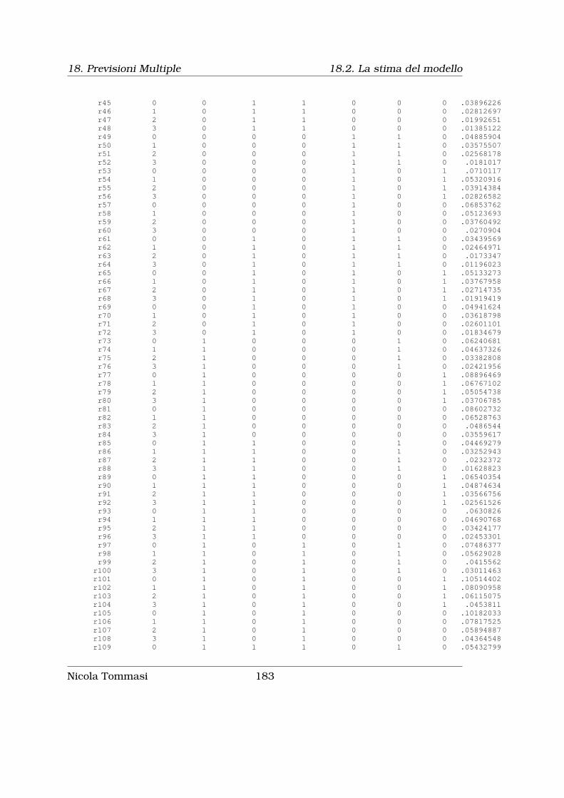
18. Previsioni Multiple 18.2. La stima del modello
r45 0 0 1 1 0 0 0 .03896226r46 1 0 1 1 0 0 0 .02812697r47 2 0 1 1 0 0 0 .01992651r48 3 0 1 1 0 0 0 .01385122r49 0 0 0 0 1 1 0 .04885904r50 1 0 0 0 1 1 0 .03575507r51 2 0 0 0 1 1 0 .02568178r52 3 0 0 0 1 1 0 .0181017r53 0 0 0 0 1 0 1 .0710117r54 1 0 0 0 1 0 1 .05320916r55 2 0 0 0 1 0 1 .03914384r56 3 0 0 0 1 0 1 .02826582r57 0 0 0 0 1 0 0 .06853762r58 1 0 0 0 1 0 0 .05123693r59 2 0 0 0 1 0 0 .03760492r60 3 0 0 0 1 0 0 .0270904r61 0 0 1 0 1 1 0 .03439569r62 1 0 1 0 1 1 0 .02464971r63 2 0 1 0 1 1 0 .0173347r64 3 0 1 0 1 1 0 .01196023r65 0 0 1 0 1 0 1 .05133273r66 1 0 1 0 1 0 1 .03767958r67 2 0 1 0 1 0 1 .02714735r68 3 0 1 0 1 0 1 .01919419r69 0 0 1 0 1 0 0 .04941624r70 1 0 1 0 1 0 0 .03618798r71 2 0 1 0 1 0 0 .02601101r72 3 0 1 0 1 0 0 .01834679r73 0 1 0 0 0 1 0 .06240681r74 1 1 0 0 0 1 0 .04637326r75 2 1 0 0 0 1 0 .03382808r76 3 1 0 0 0 1 0 .02421956r77 0 1 0 0 0 0 1 .08896469r78 1 1 0 0 0 0 1 .06767102r79 2 1 0 0 0 0 1 .05054738r80 3 1 0 0 0 0 1 .03706785r81 0 1 0 0 0 0 0 .08602732r82 1 1 0 0 0 0 0 .06528763r83 2 1 0 0 0 0 0 .0486544r84 3 1 0 0 0 0 0 .03559617r85 0 1 1 0 0 1 0 .04469279r86 1 1 1 0 0 1 0 .03252943r87 2 1 1 0 0 1 0 .0232372r88 3 1 1 0 0 1 0 .01628823r89 0 1 1 0 0 0 1 .06540354r90 1 1 1 0 0 0 1 .04874634r91 2 1 1 0 0 0 1 .03566756r92 3 1 1 0 0 0 1 .02561526r93 0 1 1 0 0 0 0 .0630826r94 1 1 1 0 0 0 0 .04690768r95 2 1 1 0 0 0 0 .03424177r96 3 1 1 0 0 0 0 .02453301r97 0 1 0 1 0 1 0 .07486377r98 1 1 0 1 0 1 0 .05629028r99 2 1 0 1 0 1 0 .0415562r100 3 1 0 1 0 1 0 .03011463r101 0 1 0 1 0 0 1 .10514402r102 1 1 0 1 0 0 1 .08090958r103 2 1 0 1 0 0 1 .06115075r104 3 1 0 1 0 0 1 .0453811r105 0 1 0 1 0 0 0 .10182033r106 1 1 0 1 0 0 0 .07817525r107 2 1 0 1 0 0 0 .05894887r108 3 1 0 1 0 0 0 .04364548r109 0 1 1 1 0 1 0 .05432799
Nicola Tommasi 183

18.2. La stima del modello 18. Previsioni Multiple
r110 1 1 1 1 0 1 0 .04001869r111 2 1 1 1 0 1 0 .02893543r112 3 1 1 1 0 1 0 .02053213r113 0 1 1 1 0 0 1 .07830834r114 1 1 1 1 0 0 1 .0590559r115 2 1 1 1 0 0 1 .04372974r116 3 1 1 1 0 0 1 .03178672r117 0 1 1 1 0 0 0 .07564123r118 1 1 1 1 0 0 0 .05691365r119 2 1 1 1 0 0 0 .04204545r120 3 1 1 1 0 0 0 .0304905r121 0 1 0 0 1 1 0 .09205978r122 1 1 0 0 1 1 0 .07018927r123 2 1 0 0 1 1 0 .05255296r124 3 1 0 0 1 1 0 .03863135r125 0 1 0 0 1 0 1 .12704809r126 1 1 0 0 1 0 1 .09910604r127 2 1 0 0 1 0 1 .07594781r128 3 1 0 0 1 0 1 .05715961r129 0 1 0 0 1 0 0 .12324235r130 1 1 0 0 1 0 0 .09592332r131 2 1 0 0 1 0 0 .07334241r132 3 1 0 0 1 0 0 .05507191r133 0 1 1 0 1 1 0 .06785662r134 1 1 1 0 1 1 0 .05069501r135 2 1 1 0 1 1 0 .03718279r136 3 1 1 0 1 1 0 .02676854r137 0 1 1 0 1 0 1 .09607838r138 1 1 1 0 1 0 1 .07346918r139 2 1 1 0 1 0 1 .05517336r140 3 1 1 0 1 0 1 .04068058r141 0 1 1 0 1 0 0 .09296776r142 1 1 1 0 1 0 0 .07092933r143 2 1 1 0 1 0 0 .05314341r144 3 1 1 0 1 0 0 .03909247r145 0 1 1 1 1 1 1 .08393377r146 0 0 0 1 1 0 1 .08473428r147 0 0 1 1 0 1 1 .02783366r148 0 0 0 0 0 1 1 .03257362r149 0 1 0 0 0 1 1 .06470847r150 0 1 1 0 1 1 1 .07031184r151 0 0 1 1 1 1 0 .04222742r152 0 1 1 1 1 0 0 .10966442r153 0 1 0 1 1 1 0 .10864002r154 0 1 1 1 0 1 1 .05639349r155 0 0 1 1 1 1 1 .04391757r156 0 1 0 1 0 1 1 .07751009r157 0 1 1 1 1 1 0 .08112232r158 0 1 0 1 1 1 1 .11212215r159 0 0 0 1 0 1 1 .04007105r160 0 0 0 1 1 1 1 .0613959r161 0 0 1 0 1 1 1 .03582672r162 0 0 0 0 1 1 1 .05075834r163 0 1 0 1 1 0 1 .14776383r164 0 1 0 0 1 1 1 .09514806r165 0 1 1 1 1 0 1 .11316993r166 0 0 0 1 1 1 0 .05918708r167 0 0 0 1 1 0 0 .08190262r168 0 1 0 1 1 0 0 .14354074r169 0 0 1 1 1 0 1 .06206314r170 0 0 1 1 1 0 0 .0598355r171 0 0 1 0 0 1 1 .02232083r172 0 1 1 0 0 1 1 .04646172r173 1 0 0 1 1 1 0 .04383302r174 1 0 1 1 1 1 0 .03063037
184 Nicola Tommasi

18. Previsioni Multiple 18.2. La stima del modello
r175 1 0 0 0 1 1 1 .0372321r176 1 0 0 1 1 0 1 .06424052r177 1 0 0 1 1 1 1 .04557462r178 1 0 1 1 1 1 1 .03193149r179 1 1 0 1 1 1 1 .08667391r180 1 1 1 1 1 1 0 .06132231r181 1 1 1 0 0 1 1 .03389654r182 1 1 0 1 0 1 1 .05841413r183 1 0 1 0 1 1 1 .02573625r184 1 1 0 0 1 1 1 .07270885r185 1 0 1 1 1 0 1 .04610165r186 1 0 0 0 0 1 1 .02327058r187 1 0 1 1 1 0 0 .04434379r188 1 1 0 1 1 0 1 .11657615r189 1 0 1 1 0 1 1 .01970707r190 1 0 1 0 0 1 1 .01561142r191 1 0 0 1 0 1 1 .02897554r192 1 1 0 1 1 0 0 .11299532r193 1 1 1 1 0 1 1 .04163717r194 1 1 1 1 1 0 1 .08754214r195 1 1 0 0 0 1 1 .04819519r196 1 1 0 1 1 1 0 .08379353r197 1 0 0 1 1 0 0 .06195188r198 1 1 1 1 1 1 1 .0635929r199 1 1 1 0 1 1 1 .05265072r200 1 1 1 1 1 0 0 .08464009r201 2 1 0 0 1 1 1 .0545651r202 2 0 0 1 1 0 0 .04601374r203 2 1 1 1 1 0 1 .06651596r204 2 1 1 0 1 1 1 .03870767r205 2 0 1 0 0 1 1 .01071203r206 2 0 0 1 1 1 1 .03321049r207 2 1 1 0 0 1 1 .02427141r208 2 1 1 1 1 0 0 .0641643r209 2 0 1 1 0 1 1 .01369051r210 2 0 1 0 1 1 1 .01814223r211 2 1 1 1 1 1 0 .04551652r212 2 1 1 1 1 1 1 .04731152r213 2 0 1 1 1 1 1 .02278574r214 2 0 0 0 0 1 1 .01631292r215 2 0 1 1 1 1 0 .02180528r216 2 1 0 1 0 1 1 .04322468r217 2 0 1 1 1 0 0 .03226015r218 2 1 0 1 1 1 1 .06581173r219 2 1 0 1 1 1 0 .06347949r220 2 1 0 0 0 1 1 .03523976r221 2 0 0 0 1 1 1 .02680613r222 2 1 0 1 1 0 0 .0873974r223 2 1 0 1 1 0 1 .09036943r224 2 1 1 1 0 1 1 .03017682r225 2 0 0 1 1 0 1 .04782438r226 2 0 0 1 1 1 0 .03186632r227 2 0 0 1 0 1 1 .0205622r228 2 0 1 1 1 0 1 .03361796r229 3 0 1 1 1 1 0 .0152314r230 3 1 1 1 1 0 0 .04776399r231 3 0 0 1 1 0 0 .03354997r232 3 1 1 0 1 1 1 .02793236r233 3 0 1 1 1 0 0 .02303382r234 3 1 0 0 0 1 1 .02529023r235 3 1 0 1 1 0 1 .06881309r236 3 1 1 1 1 1 0 .03316559r237 3 0 1 0 1 1 1 .01254771r238 3 1 1 1 0 1 1 .02146415r239 3 0 0 0 0 1 1 .01121921
Nicola Tommasi 185
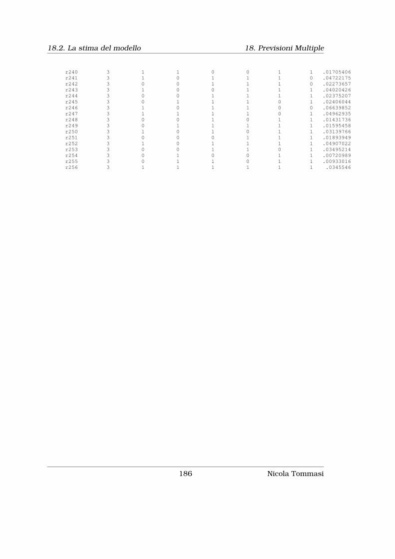
18.2. La stima del modello 18. Previsioni Multiple
r240 3 1 1 0 0 1 1 .01705406r241 3 1 0 1 1 1 0 .04722175r242 3 0 0 1 1 1 0 .02273657r243 3 1 0 0 1 1 1 .04020426r244 3 0 0 1 1 1 1 .02375207r245 3 0 1 1 1 0 1 .02406044r246 3 1 0 1 1 0 0 .06639852r247 3 1 1 1 1 0 1 .04962935r248 3 0 0 1 0 1 1 .01431736r249 3 0 1 1 1 1 1 .01595458r250 3 1 0 1 0 1 1 .03139766r251 3 0 0 0 1 1 1 .01893949r252 3 1 0 1 1 1 1 .04907022r253 3 0 0 1 1 0 1 .03495214r254 3 0 1 0 0 1 1 .00720989r255 3 0 1 1 0 1 1 .00933016r256 3 1 1 1 1 1 1 .0345546
186 Nicola Tommasi
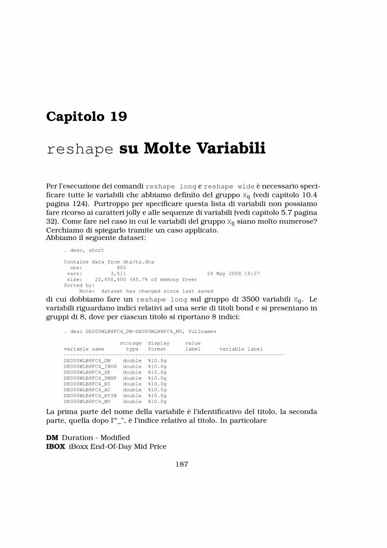
Capitolo 19
reshape su Molte Variabili
Per l’esecuzione dei comandi reshape long e reshape wide è necessario speci-ficare tutte le variabili che abbiamo definito del gruppo Xij (vedi capitolo 10.4pagina 124). Purtroppo per specificare questa lista di variabili non possiamofare ricorso ai caratteri jolly e alle sequenze di variabili (vedi capitolo 5.7 pagina32). Come fare nel caso in cui le variabili del gruppo Xij siano molto numerose?Cerchiamo di spiegarlo tramite un caso applicato.Abbiamo il seguente dataset:
. desc, short
Contains data from dta/ts.dtaobs: 800vars: 3,511 24 May 2008 10:27size: 22,450,400 (85.7% of memory free)Sorted by:
Note: dataset has changed since last saved
di cui dobbiamo fare un reshape long sul gruppo di 3500 variabili Xij. Levariabili riguardano indici relativi ad una serie di titoli bond e si presentano ingruppi di 8, dove per ciascun titolo si riportano 8 indici:
. desc DE000WLB8FC4_DM-DE000WLB8FC4_MV, fullnames
storage display valuevariable name type format label variable label-----------------------------------------------------------------------DE000WLB8FC4_DM double %10.0gDE000WLB8FC4_IBOX double %10.0gDE000WLB8FC4_SP double %10.0gDE000WLB8FC4_SWSP double %10.0gDE000WLB8FC4_RI double %10.0gDE000WLB8FC4_AC double %10.0gDE000WLB8FC4_RYIB double %10.0gDE000WLB8FC4_MV double %10.0g
La prima parte del nome della variabile è l’identificativo del titolo, la secondaparte, quella dopo l’“_”, è l’indice relativo al titolo. In particolare
DM Duration - ModifiedIBOX iBoxx End-Of-Day Mid Price
187

19. reshape su Molte Variabili
SP Spread Over Benchmark CurveSWSP Spread Over Swap CurveRI Total Return IndexAC Accrued InterestRYIB IBoxx - YieldMV Market Value (Capital)
e rappresentano l’elemento j. Teoricamente si dovrebbe fare il reshape scriven-do circa 440 variabili!. Con questo pezzo di codice però riesco ad ottenere lalista che mi serve:
preserve;keep *_AC;
renvars , postsub(_AC _);
ds *_;di "`r(varlist)'";restore;
Analizziamolo. Con keep *_AC prendo una sola occorrenza tra le 8 di cias-cun titolo, quindi elimino la parte terminale AC del nome delle variabili. Conil comando ds ottengo la lista delle variabili che vengono salvare nella localr(varlist)
. di "`r(varlist)'";DE000WLB8FC4_ XS0308936037_ DE000A0NUMG1_ XS0222695008_ XS0188> 568751_ DE0009168062_ DE0007009482_ DE000A0DXH13_ DE000A0DAL
(output omitted )
> 0185415139_ XS0173128983_ XS0328609580_ XS0312464158_
Ok ci siamo; la variabile data è l’elemento i, indichiamo con tipo l’elementoj e aggiungiamo l’opzione string dato che l’identificativo Xij non è numerico:
. reshape long "`r(varlist)'" , i(data) j(tipo) string;(note: j = AC DM IBOX MV RI RYIB SP SWSP)(note: ES0312342001_DM not found)(note: ES0312298005_DM not found)(note: DE000LBW6062_DM not found)(note: ES0312342001_IBOX not found)(note: ES0312298005_IBOX not found)(note: ES0370148001_IBOX not found)(note: DE000LBW6062_IBOX not found)(note: DE000LBW3DR8_IBOX not found)(note: DE000HBE0D55_IBOX not found)(note: DE000WLB6EG2_IBOX not found)(note: XS0282598167_IBOX not found)(note: DE000NWB2846_IBOX not found)(note: DE000DHY1149_IBOX not found)(note: DE000MHB3018_IBOX not found)(note: DE000LBW6062_MV not found)(note: DE000LBW6062_RI not found)(note: ES0312342001_RYIB not found)(note: ES0312298005_RYIB not found)(note: ES0370148001_RYIB not found)(note: DE000LBW6062_RYIB not found)(note: DE000LBW3DR8_RYIB not found)(note: DE000HBE0D55_RYIB not found)
188 Nicola Tommasi
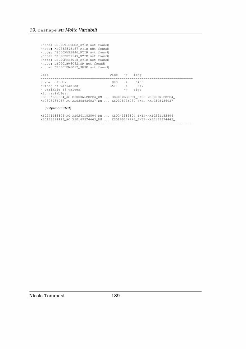
19. reshape su Molte Variabili
(note: DE000WLB6EG2_RYIB not found)(note: XS0282598167_RYIB not found)(note: DE000NWB2846_RYIB not found)(note: DE000DHY1149_RYIB not found)(note: DE000MHB3018_RYIB not found)(note: DE000LBW6062_SP not found)(note: DE000LBW6062_SWSP not found)
Data wide -> long-----------------------------------------------------------------------------Number of obs. 800 -> 6400Number of variables 3511 -> 447j variable (8 values) -> tipoxij variables:DE000WLB8FC4_AC DE000WLB8FC4_DM ... DE000WLB8FC4_SWSP->DE000WLB8FC4_XS0308936037_AC XS0308936037_DM ... XS0308936037_SWSP->XS0308936037_
(output omitted )
XS0241183804_AC XS0241183804_DM ... XS0241183804_SWSP->XS0241183804_XS0169374443_AC XS0169374443_DM ... XS0169374443_SWSP->XS0169374443_-----------------------------------------------------------------------------
Nicola Tommasi 189


Parte III
Appendici
191

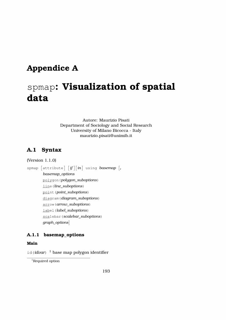
Appendice A
spmap: Visualization of spatialdata
Autore: Maurizio PisatiDepartment of Sociology and Social Research
University of Milano Bicocca - [email protected]
A.1 Syntax
(Version 1.1.0)
spmap[attribute
] [if
][in
]using basemap
[,
basemap_options
polygon(polygon_suboptions)
line(line_suboptions)
point(point_suboptions)
diagram(diagram_suboptions)
arrow(arrow_suboptions)
label(label_suboptions)
scalebar(scalebar_suboptions)
graph_options]
A.1.1 basemap_options
Main
id(idvar) 1 base map polygon identifier
1Required option
193
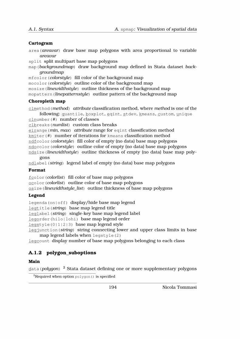
A.1. Syntax A. spmap: Visualization of spatial data
Cartogram
area(areavar) draw base map polygons with area proportional to variableareavar
split split multipart base map polygonsmap(backgroundmap) draw background map defined in Stata dataset back-
groundmapmfcolor(colorstyle) fill color of the background mapmocolor(colorstyle) outline color of the background mapmosize(linewidthstyle) outline thickness of the background mapmopattern(linepatternstyle) outline pattern of the background map
Choropleth map
clmethod(method) attribute classification method, where method is one of thefollowing: quantile, boxplot, eqint, stdev, kmeans, custom, unique
clnumber(#) number of classesclbreaks(numlist) custom class breakseirange(min, max) attribute range for eqint classification methodkmiter(#) number of iterations for kmeans classification methodndfcolor(colorstyle) fill color of empty (no data) base map polygonsndocolor(colorstyle) outline color of empty (no data) base map polygonsndsize(linewidthstyle) outline thickness of empty (no data) base map poly-
gonsndlabel(string) legend label of empty (no data) base map polygons
Format
fcolor(colorlist) fill color of base map polygonsocolor(colorlist) outline color of base map polygonsosize(linewidthstyle_list) outline thickness of base map polygons
Legend
legenda(on|off) display/hide base map legendlegtitle(string) base map legend titleleglabel(string) single-key base map legend labellegorder(hilo|lohi) base map legend orderlegstyle(0|1|2|3) base map legend stylelegjunction(string) string connecting lower and upper class limits in base
map legend labels when legstyle(2)legcount display number of base map polygons belonging to each class
A.1.2 polygon_suboptions
Main
data(polygon) 2 Stata dataset defining one or more supplementary polygons2Required when option polygon() is specified
194 Nicola Tommasi

A. spmap: Visualization of spatial data A.1. Syntax
to be superimposed onto the base mapselect(command) keep/drop specified records of dataset polygonby(byvar_pl) group supplementary polygons by variable byvar_pl
Format
fcolor(colorlist) fill color of supplementary polygonsocolor(colorlist) outline color of supplementary polygonsosize(linewidthstyle_list) outline thickness of supplementary polygons
Legend
legenda(on|off) display/hide supplementary-polygon legendlegtitle(string) supplementary-polygon legend titleleglabel(string) single-key supplementary-polygon legend labellegshow(numlist) display only selected keys of supplementary-polygon legendlegcount display number of supplementary polygons belonging to each group
A.1.3 line_suboptions
Main
data(line) 3 Stata dataset defining one or more polylines to be superimposedonto the base map
select(command) keep/drop specified records of dataset lineby(byvar_ln) group polylines by variable byvar_ln
Format
color(colorlist) polyline colorsize(linewidthstyle_list) polyline thicknesspattern(linepatternstyle_list) polyline pattern
Legend
legenda(on|off) display/hide polyline legendlegtitle(string) polyline legend titleleglabel(string) single-key polyline legend labellegshow(numlist) display only selected keys of polyline legendlegcount display number of polylines belonging to each group
A.1.4 point_suboptions
Main
data(point) Stata dataset defining one or more points to be superimposedonto the base map
3Required when option line() is specified
Nicola Tommasi 195

A.1. Syntax A. spmap: Visualization of spatial data
select(command) keep/drop specified records of dataset pointby(byvar_pn) group points by variable byvar_pnxcoord(xvar_pn) 4 variable containing the x-coordinate of pointsycoord(yvar_pn) 5 variable containing the y-coordinate of points
Proportional size
proportional(propvar_pn) draw point markers with size proportional to vari-able propvar_pn
prange(min, max) normalization range of variable propvar_pnpsize(relative|absolute) reference system for drawing point markers
Deviation
deviation(devvar_pn) draw point markers as deviations from given referencevalue of variable devvar_pn
refval(mean|median|#) reference value of variable devvar_pnrefweight(weightvar_pn) compute reference value of variable devvar_pn weight-
ing observations by variable weightvar_pndmax(#) absolute value of maximum deviation
Format
size(markersizestyle_list) size of point markersshape(symbolstyle_list) shape of point markersfcolor(colorlist) fill color of point markersocolor(colorlist) outline color of point markersosize(linewidthstyle_list) outline thickness of point markers
Legend
legenda(on|off) display/hide point legendlegtitle(string) point legend titleleglabel(string) single-key point legend labellegshow(numlist) display only selected keys of point legendlegcount display number of points belonging to each group
A.1.5 diagram_suboptions
Main
data(diagram) Stata dataset defining one or more diagrams to be superim-posed onto the base map at given reference points
select(command) keep/drop specified records of dataset diagramby(byvar_dg) group diagrams by variable byvar_dg
4Required when option point() is specified5Required when option point() is specified
196 Nicola Tommasi

A. spmap: Visualization of spatial data A.1. Syntax
xcoord(xvar_dg) 6 variable containing the x-coordinate of diagram referencepoints
ycoord(yvar_dg) 7 variable containing the y-coordinate of diagram referencepoints
variables(diagvar_dg) 8 variable or variables to be represented by diagramstype(frect|pie) diagram type
Proportional size
proportional(propvar_dg) draw diagrams with area proportional to variablepropvar_dg
prange(min, max) reference range of variable propvar_dg
Framed-rectangle chart
range(min, max) reference range of variable diagvar_dgrefval(mean|median|#) reference value of variable diagvar_dgrefweight(weightvar_dg) compute the reference value of variable diagvar_dg
weighting observations by variable weightvar_dgrefcolor(colorstyle) color of the line representing the reference value of vari-
able diagvar_dgrefsize(linewidthstyle) thickness of the line representing the reference value
of variable diagvar_dg
Format
size(#) diagram sizefcolor(colorlist) fill color of the diagramsocolor(colorlist) outline color of the diagramsosize(linewidthstyle_list) outline thickness of the diagrams
Legend
legenda(on|off) display/hide diagram legendlegtitle(string) diagram legend titlelegshow(numlist) display only selected keys of diagram legendlegcount display number of diagrams belonging to each group
A.1.6 arrow_suboptions
Main
data(arrow) 9 Stata dataset defining one or more arrows to be superimposedonto the base map
6Required when option diagram() is specified7Required when option diagram() is specified8Required when option diagram() is specified9Required when option arrow() is specified
Nicola Tommasi 197
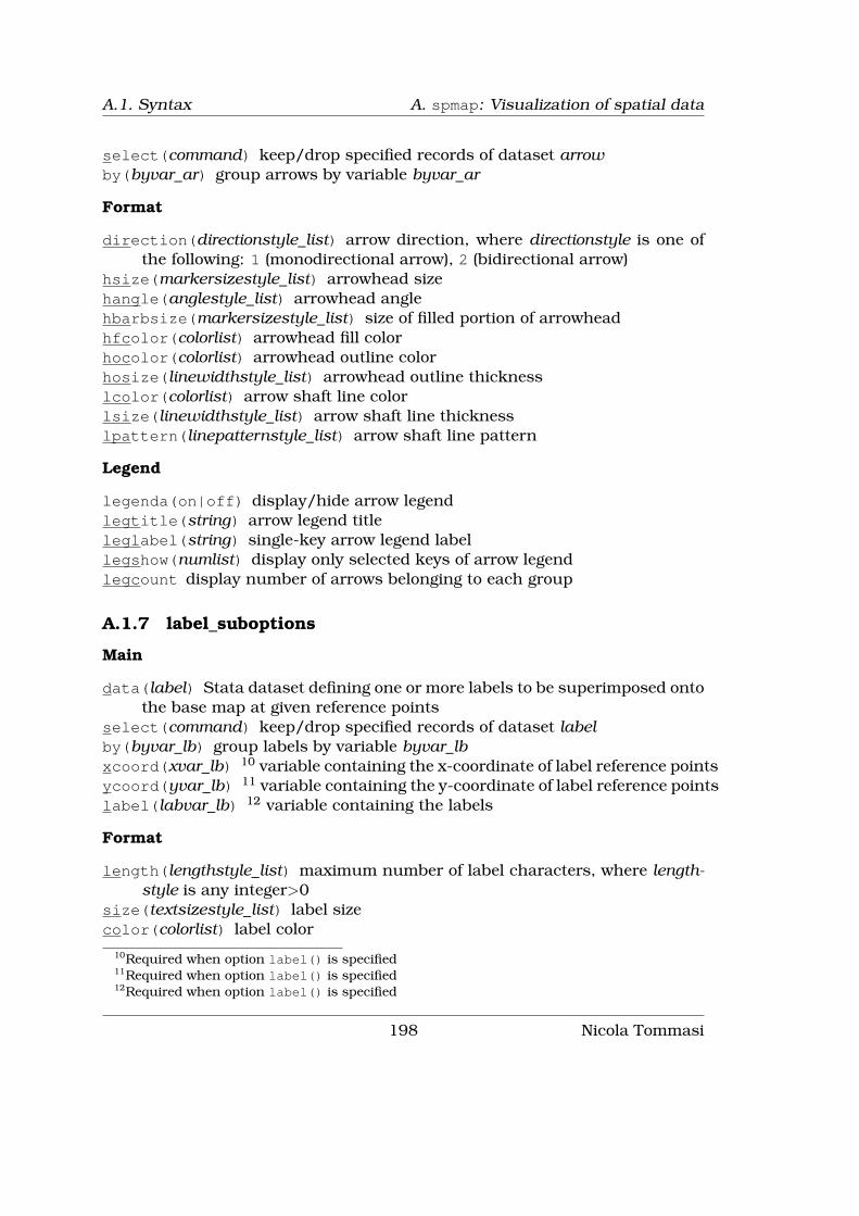
A.1. Syntax A. spmap: Visualization of spatial data
select(command) keep/drop specified records of dataset arrowby(byvar_ar) group arrows by variable byvar_ar
Format
direction(directionstyle_list) arrow direction, where directionstyle is one ofthe following: 1 (monodirectional arrow), 2 (bidirectional arrow)
hsize(markersizestyle_list) arrowhead sizehangle(anglestyle_list) arrowhead anglehbarbsize(markersizestyle_list) size of filled portion of arrowheadhfcolor(colorlist) arrowhead fill colorhocolor(colorlist) arrowhead outline colorhosize(linewidthstyle_list) arrowhead outline thicknesslcolor(colorlist) arrow shaft line colorlsize(linewidthstyle_list) arrow shaft line thicknesslpattern(linepatternstyle_list) arrow shaft line pattern
Legend
legenda(on|off) display/hide arrow legendlegtitle(string) arrow legend titleleglabel(string) single-key arrow legend labellegshow(numlist) display only selected keys of arrow legendlegcount display number of arrows belonging to each group
A.1.7 label_suboptions
Main
data(label) Stata dataset defining one or more labels to be superimposed ontothe base map at given reference points
select(command) keep/drop specified records of dataset labelby(byvar_lb) group labels by variable byvar_lbxcoord(xvar_lb) 10 variable containing the x-coordinate of label reference pointsycoord(yvar_lb) 11 variable containing the y-coordinate of label reference pointslabel(labvar_lb) 12 variable containing the labels
Format
length(lengthstyle_list) maximum number of label characters, where length-style is any integer>0
size(textsizestyle_list) label sizecolor(colorlist) label color
10Required when option label() is specified11Required when option label() is specified12Required when option label() is specified
198 Nicola Tommasi

A. spmap: Visualization of spatial data A.2. description
position(clockpos_list) position of labels relative to their reference pointgap(relativesize_list) gap between labels and their reference pointangle(anglestyle_list) label angle
A.1.8 scalebar_suboptions
Main
units(#) 13 scale bar extentscale(#) ratio of scale bar units to map unitsxpos(#) scale bar horizontal position relative to plot region centerypos(#) scale bar vertical position relative to plot region center
Format
size(#) scale bar height multiplierfcolor(colorstyle) fill color of scale barocolor(colorstyle) outline color of scale barosize(linewidthstyle) outline thickness of scale barlabel(string) scale bar labeltcolor(colorstyle) color of scale bar texttsize(textsizestyle) size of scale bar text
A.1.9 graph_options
Main
polyfirst draw supplementary polygons before the base mapgsize(#) length of shortest side of available area (in inches)freestyle ignore built-in graph formatting presets and restrictionstwoway_options any options documented in [G] twoway_options, except for ax-
is_options, aspect_option, scheme_option, by_option, and advanced_options
A.2 description
spmap is aimed at visualizing several kinds of spatial data, and is particularlysuited for drawing thematic maps and displaying the results of spatial dataanalyses.
spmap functioning rests on three basic principles:
- First, a base map representing a given region of interest R made up of Npolygons is drawn.
13Required when option scalebar() is specified
Nicola Tommasi 199

A.3. Spatial data format A. spmap: Visualization of spatial data
- Second, at the user’s choice, one or more kinds of additional spatial ob-jects may be superimposed onto the base map. In the current version ofspmap, six different kinds of spatial objects can be superimposed onto thebase map: polygons (via option polygon()), polylines (via option line()),points (via option point()), diagrams (via option diagram()), arrows (viaoption arrow()), and labels (via option label()).
- Third, at the user’s choice, one or more additional map elements may beadded, such as a scale bar (via option scalebar()), a title, a subtitle, anote, and a caption (via title_options).
Proper specification of spmap options and suboptions, combined with the avail-ability of properly formatted spatial data, allows the user to draw several kindsof maps, including choropleth maps, proportional symbol maps, pin maps, piechart maps, and noncontiguous area cartograms.
While providing sensible defaults for most options and supoptions, spmap givesthe user full control over the formatting of almost every map element, thusallowing the production of highly customized maps.
A.3 Spatial data format
spmap requires that the spatial data to be visualized be arranged into properlyformatted Stata datasets. Such datasets can be classified into nine categories:master, basemap, backgroundmap, polygon, line, point, diagram, arrow, label.
The master dataset is the dataset that resides in memory when spmap is in-voked. At the minimum, it must contain variable idvar, a numeric variablethat uniquely identifies the polygon or polygons making up the base map. Ifa choropleth map is to be drawn, then the master dataset should contain alsovariable attribute, a numeric variable expressing the values of the feature tobe represented. Additionally, if a noncontiguous area cartogram is to be drawn- i.e., if the polygons making up the base map are to be drawn with area pro-portional to the values of a given numeric variable areavar - then the masterdataset should contain also variable areavar.A basemap dataset is a Stata dataset that contains the definition of the polygonor polygons making up the base map. A basemap dataset is required to havethe following structure:
_ID _X _Y _EMBEDDED-------------------------------------
1 . . 01 10 30 01 10 50 0
200 Nicola Tommasi

A. spmap: Visualization of spatial data A.3. Spatial data format
1 30 50 01 30 30 01 10 30 02 . . 02 10 10 02 10 30 02 18 30 02 18 10 02 10 10 02 . . 02 22 10 02 22 30 02 30 30 02 30 10 02 22 10 03 . . 13 15 35 13 15 45 13 25 45 13 25 35 13 15 35 1
-------------------------------------
_ID is required and is a numeric variable that uniquely identifies the poly-gons making up the base map. _X is required and is a numeric variable thatcontains the x-coordinate of the nodes of the base map polygons. _Y is re-quired and is a numeric variable that contains the y-coordinate of the nodes ofthe base map polygons. Finally, _EMBEDDED is optional and is an indicatorvariable taking value 1 if the corresponding polygon is completely enclosed inanother polygon, and value 0 otherwise. The following should be noticed:
- Both simple and multipart polygons are allowed. In the example above,polygons 1 and 3 are simple (i.e., they consist of a single area), whilepolygon 2 is multipart (i.e., it consists of two distinct areas).
- The first record of each simple polygon or of each part of a multipartpolygon must contain missing x- and y-coordinates.
- The non-missing coordinates of each simple polygon or of each part ofa multipart polygon must be ordered so as to correspond to consecutivenodes.
- Each simple polygon or each part of a multipart polygon must be “closed”,i.e., the last pair of non-missing coordinates must be equal to the firstpair.
Nicola Tommasi 201
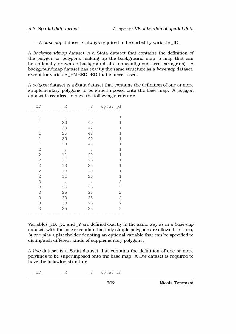
A.3. Spatial data format A. spmap: Visualization of spatial data
- A basemap dataset is always required to be sorted by variable _ID.
A backgroundmap dataset is a Stata dataset that contains the definition ofthe polygon or polygons making up the background map (a map that canbe optionally drawn as background of a noncontiguous area cartogram). Abackgroundmap dataset has exactly the same structure as a basemap dataset,except for variable _EMBEDDED that is never used.
A polygon dataset is a Stata dataset that contains the definition of one or moresupplementary polygons to be superimposed onto the base map. A polygondataset is required to have the following structure:
_ID _X _Y byvar_pl-------------------------------------
1 . . 11 20 40 11 20 42 11 25 42 11 25 40 11 20 40 12 . . 12 11 20 12 11 25 12 13 25 12 13 20 12 11 20 13 . . 23 25 25 23 25 35 23 30 35 23 30 25 23 25 25 2
-------------------------------------
Variables _ID, _X, and _Y are defined exactly in the same way as in a basemapdataset, with the sole exception that only simple polygons are allowed. In turn,byvar_pl is a placeholder denoting an optional variable that can be specified todistinguish different kinds of supplementary polygons.
A line dataset is a Stata dataset that contains the definition of one or morepolylines to be superimposed onto the base map. A line dataset is required tohave the following structure:
_ID _X _Y byvar_ln
202 Nicola Tommasi
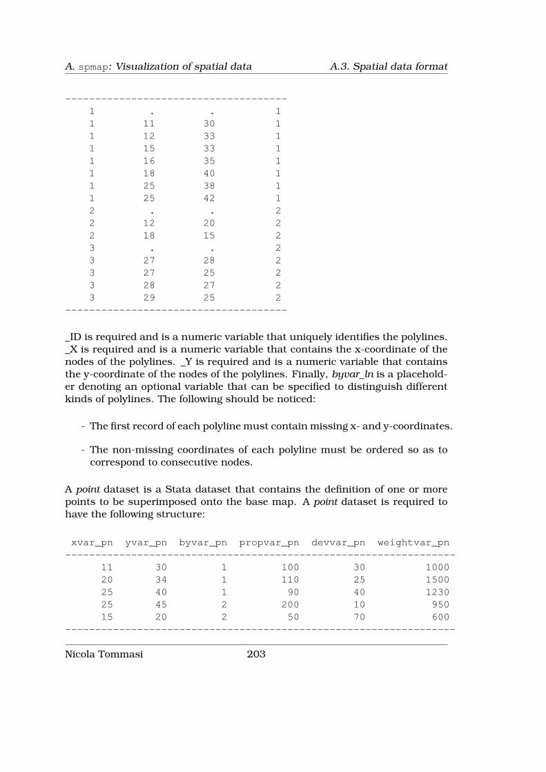
A. spmap: Visualization of spatial data A.3. Spatial data format
-------------------------------------1 . . 11 11 30 11 12 33 11 15 33 11 16 35 11 18 40 11 25 38 11 25 42 12 . . 22 12 20 22 18 15 23 . . 23 27 28 23 27 25 23 28 27 23 29 25 2
-------------------------------------
_ID is required and is a numeric variable that uniquely identifies the polylines._X is required and is a numeric variable that contains the x-coordinate of thenodes of the polylines. _Y is required and is a numeric variable that containsthe y-coordinate of the nodes of the polylines. Finally, byvar_ln is a placehold-er denoting an optional variable that can be specified to distinguish differentkinds of polylines. The following should be noticed:
- The first record of each polyline must contain missing x- and y-coordinates.
- The non-missing coordinates of each polyline must be ordered so as tocorrespond to consecutive nodes.
A point dataset is a Stata dataset that contains the definition of one or morepoints to be superimposed onto the base map. A point dataset is required tohave the following structure:
xvar_pn yvar_pn byvar_pn propvar_pn devvar_pn weightvar_pn-----------------------------------------------------------------
11 30 1 100 30 100020 34 1 110 25 150025 40 1 90 40 123025 45 2 200 10 95015 20 2 50 70 600
-----------------------------------------------------------------
Nicola Tommasi 203

A.3. Spatial data format A. spmap: Visualization of spatial data
xvar_pn is a placeholder denoting a required numeric variable that containsthe x-coordinate of the points. yvar_pn is a placeholder denoting a requirednumeric variable that contains the y-coordinate of the points. byvar_pn is aplaceholder denoting an optional variable that can be specified to distinguishdifferent kinds of points. propvar_pn is a placeholder denoting an optionalvariable that, when specified, requests that the point markers be drawn withsize proportional to propvar_pn. devvar_pn is a placeholder denoting an op-tional variable that, when specified, requests that the point markers be drawnas deviations from a given reference value of devvar_pn. Finally, weightvar_pnis a placeholder denoting an optional variable that, when specified, requeststhat the reference value of devvar_pn be computed weighting observations byvariable weightvar_pn. It is important to note that the required and optionalvariables making up a point dataset can either reside in an external dataset orbe part of the master dataset.
A diagram dataset is a Stata dataset that contains the definition of one or morediagrams to be superimposed onto the base map at given reference points. Adiagram dataset is required to have the following structure:
xvar_dg yvar_dg byvar_dg diagvar_dg propvar_dg weightvar_dg------------------------------------------------------------------
15 30 1 ... 30 100018 40 1 ... 25 150020 45 1 ... 40 123025 45 2 ... 10 95015 20 2 ... 70 600
------------------------------------------------------------------
xvar_dg is a placeholder denoting a required numeric variable that containsthe x-coordinate of the diagram reference points. yvar_dg is a placeholderdenoting a required numeric variable that contains the y-coordinate of thediagram reference points. byvar_dg is a placeholder denoting an optional vari-able that can be specified to distinguish different groups of diagrams. diag-var_dg is a placeholder denoting one or more variables to be represented bythe diagrams. propvar_dg is a placeholder denoting an optional variable that,when specified, requests that the diagrams be drawn with area proportional topropvar_dg. Finally, weightvar_dg is a placeholder denoting an optional vari-able that, when specified, requests that the reference value of the diagrams becomputed weighting observations by variable weightvar_dg (this applies only toframed-rectangle charts). It is important to note that the required and optionalvariables making up a diagram dataset can either reside in an external datasetor be part of the master dataset.
204 Nicola Tommasi

A. spmap: Visualization of spatial data A.3. Spatial data format
An arrow dataset is a Stata dataset that contains the definition of one or morearrows to be superimposed onto the base map. An arrow dataset is requiredto have the following structure:
_ID _X1 _Y1 _X2 _Y2 byvar_ar---------------------------------------------------------
1 11 30 18 30 12 15 40 15 45 13 15 40 25 40 14 20 35 28 45 25 17 20 20 11 2
---------------------------------------------------------
_ID is required and is a numeric variable that uniquely identifies the arrows._X1 is required and is a numeric variable that contains the x-coordinate ofthe starting point of the arrows. _Y1 is required and is a numeric variablethat contains the y-coordinate of the starting point of the arrows. _X2 is re-quired and is a numeric variable that contains the x-coordinate of the endingpoint of the arrows. _Y2 is required and is a numeric variable that contains they-coordinate of the ending point of the arrows. Finally, byvar_ar is a placehold-er denoting an optional variable that can be specified to distinguish differentkinds of arrows.
A label dataset is a Stata dataset that contains the definition of one or morelabels to be superimposed onto the base map at given reference points. A labeldataset is required to have the following structure:
xvar_lb yvar_lb byvar_lb labvar_lb---------------------------------------
11 33 1 Abcde20 37 1 Fgh25 43 1 IJKL25 48 2 Mnopqr15 22 2 stu
---------------------------------------
xvar_lb is a placeholder denoting a required numeric variable that contains thex-coordinate of the label reference points. yvar_lb is a placeholder denoting arequired numeric variable that contains the y-coordinate of the label referencepoints. byvar_lb is a placeholder denoting an optional variable that can bespecified to distinguish different kinds of labels. Finally, labvar_lb is a place-holder denoting the variable that contains the labels. It is important to notethat the required and optional variables making up a label dataset can eitherreside in an external dataset or be part of the master dataset.
Nicola Tommasi 205
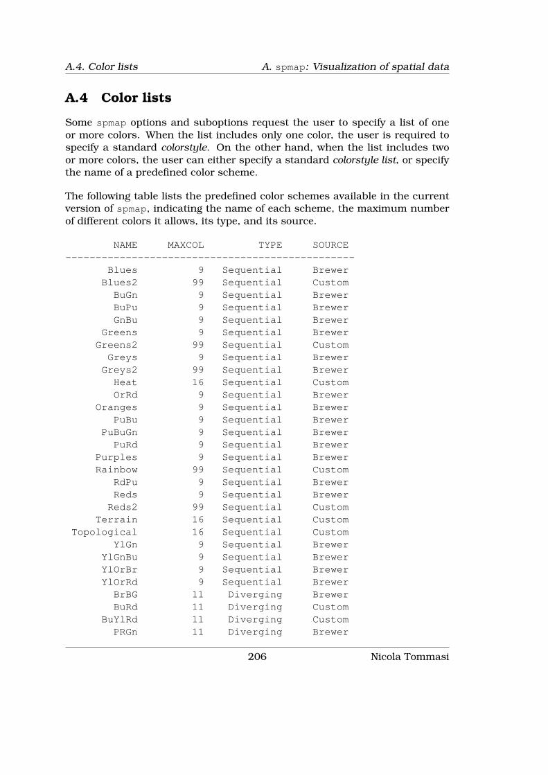
A.4. Color lists A. spmap: Visualization of spatial data
A.4 Color lists
Some spmap options and suboptions request the user to specify a list of oneor more colors. When the list includes only one color, the user is required tospecify a standard colorstyle. On the other hand, when the list includes twoor more colors, the user can either specify a standard colorstyle list, or specifythe name of a predefined color scheme.
The following table lists the predefined color schemes available in the currentversion of spmap, indicating the name of each scheme, the maximum numberof different colors it allows, its type, and its source.
NAME MAXCOL TYPE SOURCE------------------------------------------------
Blues 9 Sequential BrewerBlues2 99 Sequential CustomBuGn 9 Sequential BrewerBuPu 9 Sequential BrewerGnBu 9 Sequential Brewer
Greens 9 Sequential BrewerGreens2 99 Sequential CustomGreys 9 Sequential BrewerGreys2 99 Sequential Brewer
Heat 16 Sequential CustomOrRd 9 Sequential Brewer
Oranges 9 Sequential BrewerPuBu 9 Sequential Brewer
PuBuGn 9 Sequential BrewerPuRd 9 Sequential Brewer
Purples 9 Sequential BrewerRainbow 99 Sequential Custom
RdPu 9 Sequential BrewerReds 9 Sequential Brewer
Reds2 99 Sequential CustomTerrain 16 Sequential Custom
Topological 16 Sequential CustomYlGn 9 Sequential Brewer
YlGnBu 9 Sequential BrewerYlOrBr 9 Sequential BrewerYlOrRd 9 Sequential Brewer
BrBG 11 Diverging BrewerBuRd 11 Diverging Custom
BuYlRd 11 Diverging CustomPRGn 11 Diverging Brewer
206 Nicola Tommasi

A. spmap: Visualization of spatial data A.5. Choropleth maps
PiYG 11 Diverging BrewerPuOr 11 Diverging BrewerRdBu 11 Diverging BrewerRdGy 11 Diverging Brewer
RdYlBu 11 Diverging BrewerRdYlGn 11 Diverging Brewer
Spectral 11 Diverging BrewerAccent 8 Qualitative BrewerDark2 8 Qualitative BrewerPaired 12 Qualitative Brewer
Pastel1 9 Qualitative BrewerPastel2 8 Qualitative Brewer
Set1 9 Qualitative BrewerSet2 8 Qualitative BrewerSet3 12 Qualitative Brewer
------------------------------------------------
Following Brewer (1999), sequential schemes are typically used to representordered data, so that higher data values are represented by darker colors;in turn, diverging schemes are used when there is a meaningful midpoint inthe data, to emphasize progressive divergence from this midpoint in the twoopposite directions; finally, qualitative schemes are generally used to representunordered, categorical data.The color schemes whose source is indicated as Brewer were designed by Dr.Cynthia A. Brewer, Department of Geography, The Pennsylvania State Uni-versity, University Park, Pennsylvania, USA (Brewer et al. 2003). These col-or schemes are used with Dr. Brewer’s permission and are taken from theColorBrewer map design tool available at ColorBrewer.org.
A.5 Choropleth maps
A choropleth map can be defined as a map in which each subarea (e.g., eachcensus tract) of a given region of interest (e.g., a city) is colored or shaded withan intensity proportional to the value taken on by a given quantitative variablein that subarea (Slocum et al. 2005). Since choropleth maps are one of themost popular means for representing the spatial distribution of quantitativevariables, it is worth noting the way spmap can be used to draw this kind ofmap.In spmap, a choropleth map is a base map whose constituent polygons arecolored according to the values taken on by attribute, a numeric variable thatmust be contained in the master dataset and specified immediately after themain command (see syntax diagram above). To draw the desired choroplethmap, spmap first groups the values taken on by variable attribute into k classes
Nicola Tommasi 207
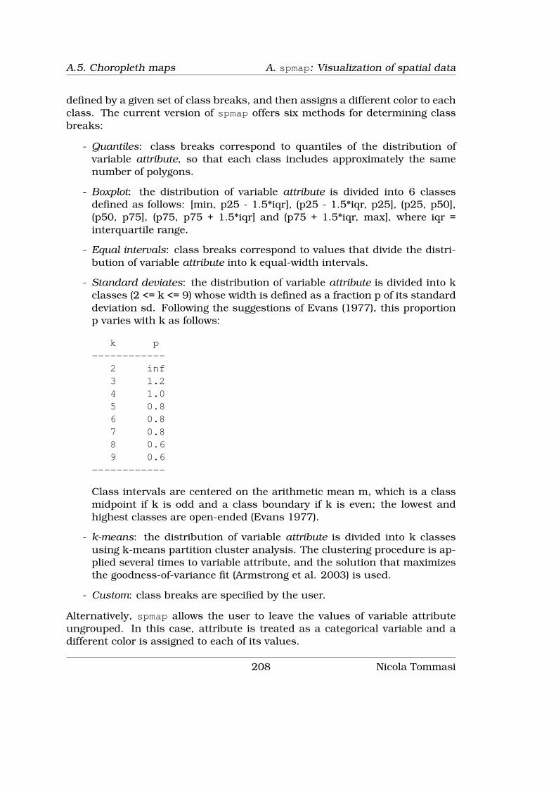
A.5. Choropleth maps A. spmap: Visualization of spatial data
defined by a given set of class breaks, and then assigns a different color to eachclass. The current version of spmap offers six methods for determining classbreaks:
- Quantiles: class breaks correspond to quantiles of the distribution ofvariable attribute, so that each class includes approximately the samenumber of polygons.
- Boxplot: the distribution of variable attribute is divided into 6 classesdefined as follows: [min, p25 - 1.5*iqr], (p25 - 1.5*iqr, p25], (p25, p50],(p50, p75], (p75, p75 + 1.5*iqr] and (p75 + 1.5*iqr, max], where iqr =interquartile range.
- Equal intervals: class breaks correspond to values that divide the distri-bution of variable attribute into k equal-width intervals.
- Standard deviates: the distribution of variable attribute is divided into kclasses (2 <= k <= 9) whose width is defined as a fraction p of its standarddeviation sd. Following the suggestions of Evans (1977), this proportionp varies with k as follows:
k p------------
2 inf3 1.24 1.05 0.86 0.87 0.88 0.69 0.6
------------
Class intervals are centered on the arithmetic mean m, which is a classmidpoint if k is odd and a class boundary if k is even; the lowest andhighest classes are open-ended (Evans 1977).
- k-means: the distribution of variable attribute is divided into k classesusing k-means partition cluster analysis. The clustering procedure is ap-plied several times to variable attribute, and the solution that maximizesthe goodness-of-variance fit (Armstrong et al. 2003) is used.
- Custom: class breaks are specified by the user.
Alternatively, spmap allows the user to leave the values of variable attributeungrouped. In this case, attribute is treated as a categorical variable and adifferent color is assigned to each of its values.
208 Nicola Tommasi

A. spmap: Visualization of spatial data A.6. Options for drawing the base map
A.6 Options for drawing the base map
Main
id(idvar) specifies the name of a numeric variable that uniquely identifies thepolygon or polygons making up the base map. idvar must be containedin the master dataset, and its values must correspond to the values takenon by variable _ID contained in the basemap dataset.
Cartogram
area(areavar) requests that the polygons making up the base map be drawnwith area proportional to the values taken on by numeric variable areavar,so that a noncontiguous area cartogram (Olson 1976) is obtained. areavarmust be contained in the master dataset.
split requests that, before drawing a noncontiguous area cartogram, all mul-tipart base map polygons be split into their constituent parts, each ofwhich will then be treated as a distinct simple polygon.
map(backgroundmap) requests that, when drawing a noncontiguous area car-togram, the polygons making up the base map be superimposed onto abackground map defined in Stata dataset backgroundmap.
mfcolor(colorstyle) specifies the fill color of the background map. The defaultis mfcolor(none).
mocolor(colorstyle) specifies the outline color of the background map. Thedefault is mocolor(black).
mosize(linewidthstyle) specifies the outline thickness of the background map.The default is mosize(thin).
mopattern(linepatternstyle) specifies the outline pattern of the backgroundmap. The default is mopattern(solid).
Choropleth map
clmethod(method) specifies the method to be used for classifying variableattribute and representing its spatial distribution as a choropleth map.
clmethod(quantile) is the default and requests that the quantiles methodbe used.
clmethod(boxplot) requests that the boxplot method be used.clmethod(eqint) requests that the equal intervals method be used.clmethod(stdev) requests that the standard deviates method be used.clmethod(kmeans) requests that the k-means method be used.clmethod(custom) requests that class breaks be specified by the user
with option clbreaks(numlist).clmethod(unique) requests that each value of variable attribute be treat-
ed as a distinct class.
Nicola Tommasi 209

A.6. Options for drawing the base map A. spmap: Visualization of spatial data
clnumber(#) specifies the number of classes k in which variable attribute isto be divided. When the quantiles, equal intervals, standard deviates,or k-means classification method is chosen, the default is clnumber(4).When the boxplot classification method is chosen, this option is inactiveand k=6. When the custom classification method is chosen, this option isinactive and k equals the number of elements of numlist specified in op-tion clbreaks(numlist) minus 1. When the unique classification methodis chosen, this option is inactive and k equals the number of differentvalues taken on by variable attribute.
clbreaks(numlist) is required when option clmethod(custom) is specified.It defines the custom class breaks to be used for classifying variable at-tribute. numlist should be specified so that the first element is the min-imum value of variable attribute to be considered; the second to kthelements are the class breaks; and the last element is the maximumvalue of variable attribute to be considered. For example, suppose wewant to group the values of variable attribute into the following fourclasses: [10,15], (15,20], (20,25] and (25,50]; for this we must specifyclbreaks(10 15 20 25 50).
eirange(min, max) specifies the range of values (minimum and maximum) tobe considered in the calculation of class breaks when option clmethod(eqint)is specified. This option overrides the default range [min(attribute), max(attribute)].
kmiter(#) specifies the number of times the clustering procedure is appliedwhen option clmethod(kmeans) is specified. The default is kmiter(20).
ndfcolor(colorstyle) specifies the fill color of the empty (no data) polygons ofthe choropleth map. The default is ndfcolor(white).
ndocolor(colorstyle) specifies the outline color of the empty (no data) poly-gons of the choropleth map. The default is ndocolor(black).
ndsize(linewidthstyle) specifies the outline thickness of the empty (no data)polygons of the choropleth map. The default is ndsize(thin).
ndlabel(string) specifies the legend label to be attached to the empty (nodata) polygons of the choropleth map. The default is ndlabel(No data).
Format
fcolor(colorlist) specifies the list of fill colors of the base map polygons.When no choropleth map is drawn, the list should include only one el-ement. On the other hand, when a choropleth map is drawn, the listshould be either composed of k elements, or represented by the name of apredefined color scheme. The default fill color is none. When a choroplethmap is drawn, the default argument is a color scheme that depends onthe classification method specified in option clmethod(method):
Classification Defaultmethod color scheme
----------------------------------
210 Nicola Tommasi

A. spmap: Visualization of spatial data A.6. Options for drawing the base map
quantile Greysboxplot BuRdeqint Greysstdev BuRdkmeans Greyscustom Greysunique Paired
----------------------------------
ocolor(colorlist) specifies the list of outline colors of the base map polygons.When no choropleth map is drawn, the list should include only one el-ement. On the other hand, when a choropleth map is drawn, the listshould be either composed of k elements, or represented by the name ofa predefined color scheme. The default outline color is black, the defaultspecification is ocolor(black ...).
osize(linewidthstyle_list) specifies the list of outline thicknesses of the basemap polygons. When no choropleth map is drawn, the list should includeonly one element. On the other hand, when a choropleth map is drawn,the list should be composed of k elements. The default outline thicknessis thin, the default specification is osize(thin ...).
Legend
legenda(on|off) specifies whether the base map legend should be displayedor hidden.
legenda(on) requests that the base map legend be displayed. This isthe default when a choropleth map is drawn.
legenda(off) requests that the base map legend be hidden. This is thedefault when no choropleth map is drawn.
legtitle(string) specifies the title of the base map legend. When a choro-pleth map is drawn, option legtitle(varlab) requests that the label ofvariable attribute be used as the legend title.
leglabel(string) specifies the label to be attached to the single key of thebase map legend when no choropleth map is drawn. This option is re-quired when option legenda(on) is specified and no choropleth map isdrawn.
legorder(hilo|lohi) specifies the display order of the keys of the base maplegend when a choropleth map is drawn.
legorder(hilo) is the default and requests that the keys of the basemap legend be displayed in descending order of variable attribute.
legorder(lohi) requests that the keys of the base map legend be dis-played in ascending order of variable attribute. This is the defaultwhen option clmethod(unique) is specified.
Nicola Tommasi 211

A.7. Option polygon() suboptions A. spmap: Visualization of spatial data
legstyle(0|1|2|3) specifies the way the keys of the base map legend arelabelled when a choropleth map is drawn.
legstyle(0) requests that the keys of the base map legend not be la-belled.
legstyle(1) is the default and requests that the keys of the base maplegend be labelled using the standard mathematical notation for val-ue intervals (e.g.: (20,35]).
legstyle(2) requests that the keys of the base map legend be labelledusing the notation ll&ul, where ll denotes the lower limit of the classinterval, ul denotes the upper limit of the class interval, and & de-notes a string that separates the two values. For example, if ll=20,ul=35, and &=“ - ”, then the resulting label will be “20 - 35”.
legstyle(3) requests that only the first and last keys of the base maplegend be labelled; the first key is labelled with the lower limit of thecorresponding class interval, the last key is labelled with the upperlimit of the corresponding class interval.
legjunction(string) specifies the string to be used as separator when optionlegstyle(2) is specified. The default is legjunction(“ - “).
legcount requests that, when a choropleth map is drawn, the number of basemap polygons belonging to each class of variable attribute be displayed inthe legend.
A.7 Option polygon() suboptions
Main
data(polygon) requests that one or more supplementary polygons defined inStata dataset polygon be superimposed onto the base map.
select(command) requests that a given subset of records of dataset polygonbe selected using Stata commands keep or drop.
by(byvar_pl) indicates that the supplementary polygons defined in datasetpolygon belong to kpl different groups specified by variable byvar_pl.
Format
fcolor(colorlist) specifies the list of fill colors of the supplementary polygons.When suboption by(byvar_pl) is not specified, the list should includeonly one element. On the other hand, when suboption by(byvar_pl) isspecified, the list should be either composed of kpl elements, or repre-sented by the name of a predefined color scheme. The default fill color isnone, the default specification is fcolor(none ...).
ocolor(colorlist) specifies the list of outline colors of the supplementary poly-gons. When suboption by(byvar_pl) is not specified, the list should in-clude only one element. On the other hand, when suboption by(byvar_pl)
212 Nicola Tommasi
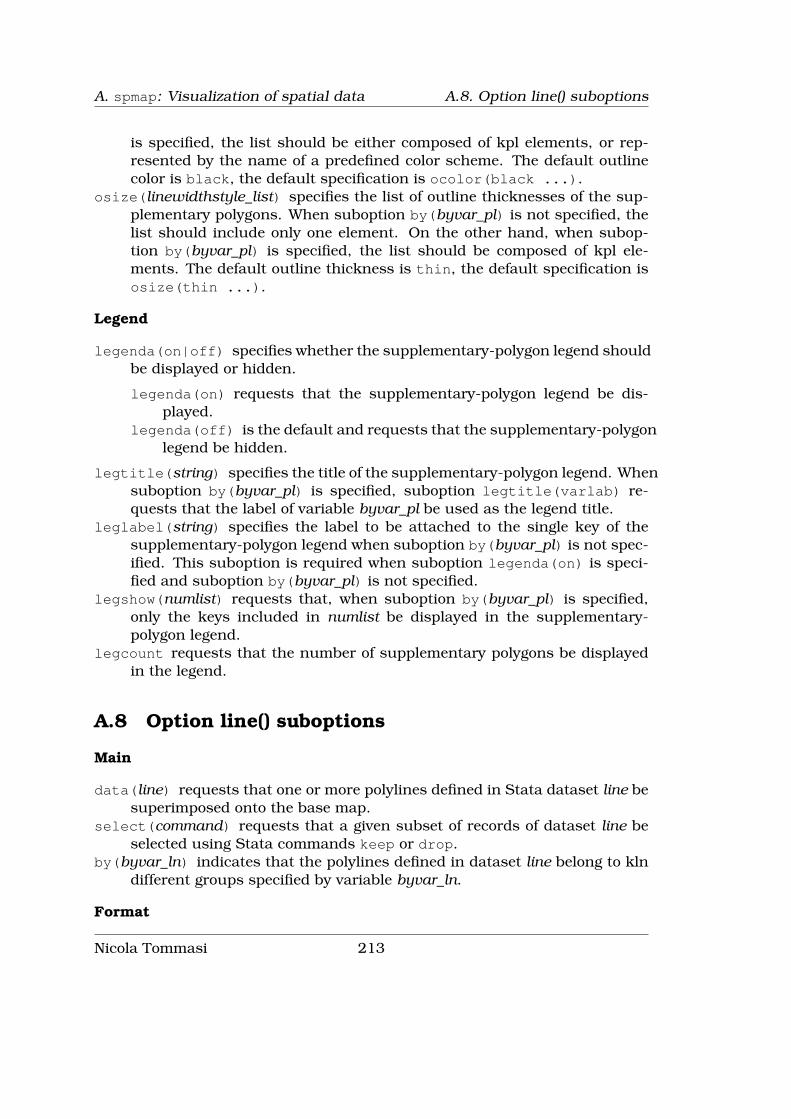
A. spmap: Visualization of spatial data A.8. Option line() suboptions
is specified, the list should be either composed of kpl elements, or rep-resented by the name of a predefined color scheme. The default outlinecolor is black, the default specification is ocolor(black ...).
osize(linewidthstyle_list) specifies the list of outline thicknesses of the sup-plementary polygons. When suboption by(byvar_pl) is not specified, thelist should include only one element. On the other hand, when subop-tion by(byvar_pl) is specified, the list should be composed of kpl ele-ments. The default outline thickness is thin, the default specification isosize(thin ...).
Legend
legenda(on|off) specifies whether the supplementary-polygon legend shouldbe displayed or hidden.
legenda(on) requests that the supplementary-polygon legend be dis-played.
legenda(off) is the default and requests that the supplementary-polygonlegend be hidden.
legtitle(string) specifies the title of the supplementary-polygon legend. Whensuboption by(byvar_pl) is specified, suboption legtitle(varlab) re-quests that the label of variable byvar_pl be used as the legend title.
leglabel(string) specifies the label to be attached to the single key of thesupplementary-polygon legend when suboption by(byvar_pl) is not spec-ified. This suboption is required when suboption legenda(on) is speci-fied and suboption by(byvar_pl) is not specified.
legshow(numlist) requests that, when suboption by(byvar_pl) is specified,only the keys included in numlist be displayed in the supplementary-polygon legend.
legcount requests that the number of supplementary polygons be displayedin the legend.
A.8 Option line() suboptions
Main
data(line) requests that one or more polylines defined in Stata dataset line besuperimposed onto the base map.
select(command) requests that a given subset of records of dataset line beselected using Stata commands keep or drop.
by(byvar_ln) indicates that the polylines defined in dataset line belong to klndifferent groups specified by variable byvar_ln.
Format
Nicola Tommasi 213

A.9. Option point() suboptions A. spmap: Visualization of spatial data
color(colorlist) specifies the list of polyline colors. When suboption by(byvar_ln)is not specified, the list should include only one element. On the otherhand, when suboption by(byvar_ln) is specified, the list should be ei-ther composed of kln elements, or represented by the name of a prede-fined color scheme. The default color is black, the default specificationis color(black ...).
size(linewidthstyle_list) specifies the list of polyline thicknesses. When sub-option by(byvar_ln) is not specified, the list should include only one ele-ment. On the other hand, when suboption by(byvar_ln) is specified, thelist should be composed of kln elements. The default thickness is thin,the default specification is size(thin ...).
pattern(linepatternstyle_list) specifies the list of polyline patterns. Whensuboption by(byvar_ln) is not specified, the list should include only oneelement. On the other hand, when suboption by(byvar_ln) is specified,the list should be composed of kln elements. The default pattern is solid,the default specification is pattern(solid ...).
Legend
legenda(on|off) specifies whether the polyline legend should be displayedor hidden.
legenda(on) requests that the polyline legend be displayed.legenda(off) is the default and requests that the polyline legend be
hidden.
legtitle(string) specifies the title of the polyline legend. When suboptionby(byvar_ln) is specified, suboption legtitle(varlab) requests thatthe label of variable (byvar_ln) be used as the legend title.
leglabel(string) specifies the label to be attached to the single key of thepolyline legend when suboption by(byvar_ln) is not specified. This sub-option is required when suboption legenda(on) is specified and subop-tion by(byvar_ln) is not specified.
legshow(numlist) requests that, when suboption by(byvar_ln) is specified,only the keys included in numlist be displayed in the polyline legend.
legcount requests that the number of polylines be displayed in the legend.
A.9 Option point() suboptions
Main
data(point) requests that one or more points defined in Stata dataset point besuperimposed onto the base map.
select(command) requests that a given subset of records of dataset point beselected using Stata commands keep or drop.
214 Nicola Tommasi

A. spmap: Visualization of spatial data A.9. Option point() suboptions
by(byvar_pn) indicates that the points defined in dataset point belong to kpndifferent groups specified by variable byvar_pn.
xcoord(xvar_pn) specifies the name of the variable containing the x-coordinateof each point.
ycoord(yvar_pn) specifies the name of the variable containing the y-coordinateof each point.
Proportional size
proportional(propvar_pn) requests that the point markers be drawn withsize proportional to the values taken on by numeric variable propvar_pn.
prange(min, max) requests that variable propvar_pn specified in suboptionproportional(propvar_pn) be normalized based on range [min, max].This suboption overrides the default normalization based on range [0,max(propvar_pn)].
psize(relative|absolute) specifies the reference system for drawing thepoint markers.
psize(relative) is the default and requests that the point markers bedrawn using relative minimum and maximum reference values. Thisis the best choice when there is no need to compare the map at handwith other maps of the same kind.
psize(absolute) requests that the point markers be drawn using ab-solute minimum and maximum reference values. This is the bestchoice when the map at hand is to be compared with other maps ofthe same kind.
Deviation
deviation(devvar_pn) requests that the point markers be drawn as devia-tions from a reference value of numeric variable devvar_pn specified inoption refval(). When this suboption is specified, in the first placethe values of variable devvar_pn are re-expressed as deviations from thechosen reference value. Then, points associated with positive deviationsare represented by solid markers, whereas points associated with neg-ative deviations are represented by hollow markers of the same shape;in both cases, markers are drawn with size proportional to the absolutevalue of the deviation. This suboption is incompatible with suboptionproportional(propvar_pn).
refval(mean|median|#) specifies the reference value of variable devvar_pnfor computing deviations.
refval(mean) is the default and requests that the arithmetic mean ofvariable devvar_pn be taken as the reference value.
refval(median) requests that the median of variable devvar_pn be tak-en as the reference value.
Nicola Tommasi 215

A.9. Option point() suboptions A. spmap: Visualization of spatial data
refval(#) requests that an arbitrary real value #be taken as the refer-ence value.
refweight(weightvar_pn) requests that the reference value of variable dev-var_pn be computed weighting observations by values of variable weight-var_pn.
dmax(#) requests that the point markers be drawn using value #as the maxi-mum absolute deviation of reference.
Format
size(markersizestyle_list) specifies the list of point marker sizes. When sub-option by(byvar_pn) is not specified, the list should include only oneelement. On the other hand, when suboption by(byvar_pn) is specified,the list should be composed of kpn elements. The default size is *1, thedefault specification is size(*1 ...).
shape(symbolstyle_list) specifies the list of point marker shapes. When sub-option by(byvar_pn) is not specified, the list should include only one ele-ment. On the other hand, when suboption by(byvar_pn) is specified, thelist should be composed of kpn elements. The default shape is o, the de-fault specification is shape(o ...). When suboption deviation(devvar_pn)is specified, this suboption accepts only solid symbolstyles written inshort form: O D T S o d t s.
fcolor(colorlist) specifies the list of fill colors of the point markers. Whensuboption by(byvar_pn) is not specified, the list should include only oneelement. On the other hand, when suboption by(byvar_pn) is specified,the list should be either composed of kpn elements, or represented by thename of a predefined color scheme. The default fill color is black, thedefault specification is fcolor(black ...).
ocolor(colorlist) specifies the list of outline colors of the point markers. Whensuboption by(byvar_pn) is not specified, the list should include only oneelement. On the other hand, when suboption by(byvar_pn) is specified,the list should be either composed of kpn elements, or represented by thename of a predefined color scheme. The default outline color is none, thedefault specification is ocolor(none ...).
osize(linewidthstyle_list) specifies the list of outline thicknesses of the pointmarkers. When suboption by(byvar_pn) is not specified, the list shouldinclude only one element. On the other hand, when suboption by(byvar_pn)is specified, the list should be composed of kpl elements. The defaultoutline thickness is thin, the default specification is osize(thin ...).
Legend
legenda(on|off) specifies whether the point legend should be displayed orhidden.
216 Nicola Tommasi

A. spmap: Visualization of spatial data A.10. Option diagram() suboptions
legenda(on) requests that the point legend be displayed.legenda(off) is the default and requests that the point legend be hid-
den.
legtitle(string) specifies the title of the point legend. When suboption by(byvar_pn)is specified, suboption legtitle(varlab) requests that the label of vari-able byvar_pn be used as the legend title.
leglabel(string) specifies the label to be attached to the single key of thepoint legend when suboption by(byvar_pn) is not specified. This subop-tion is required when suboption legenda(on) is specified and suboptionby(byvar_pn) is not specified.
legshow(numlist) requests that, when suboption by(byvar_pn) is specified,only the keys included in numlist be displayed in the point legend.
legcount requests that the number of points be displayed in the legend.
A.10 Option diagram() suboptions
Main
data(diagram) requests that one or more diagrams defined in Stata datasetdiagram be superimposed onto the base map at given reference points.
select(command) requests that a given subset of records of dataset diagrambe selected using Stata commands keep or drop.
by(byvar_dg) indicates that the diagrams defined in dataset diagram belongto kdg different groups specified by variable byvar_dg. This option is ac-tive only when just one variable is specified in suboption variables(diagvar_dg).
xcoord(xvar_dg) specifies the name of the variable containing the x-coordinateof each diagram reference point.
ycoord(yvar_dg) specifies the name of the variable containing the y-coordinateof each diagram reference point.
variables(diagvar_dg) specifies the list of variables to be represented by thediagrams.
type(frect|pie) specifies the type of diagram to be used.
type(frect) is the default when only one variable is specified in sub-option variables(diagvar_dg) and requests that framed-rectanglecharts (Cleveland and McGill 1984; Cleveland 1994) be used.
type(pie) is the default (and the only possibility) when two or morevariables are specified in suboption variables(diagvar_dg) and re-quests that pie charts be used. When option type(pie) is speci-fied, the variables specified in suboption variables(diagvar_dg) arerescaled so that they sum to 1 within each observation.
Proportional size
Nicola Tommasi 217
A.10. Option diagram() suboptions A. spmap: Visualization of spatial data
proportional(propvar_dg) requests that the diagrams be drawn with sizeproportional to the values taken on by numeric variable propvar_dg.
prange(min, max) requests that variable propvar_dg specified in suboptionproportional(propvar_dg) be normalized based on range [min, max].This suboption overrides the default normalization based on range [0,max(propvar_dg)].
Framed-rectangle chart
range(min, max) requests that variable diagvar_dg specified in suboption variables(diagvar_dg)be normalized based on range [min, max]. This suboption overrides thedefault normalization based on range [0, max(diagvar_dg)].
refval(mean|median|#) specifies the reference value of variable diagvar_dgfor drawing the reference line.
refval(mean) is the default and requests that the arithmetic mean ofvariable diagvar_dg be taken as the reference value.
refval(median) requests that the median of variable diagvar_dg be tak-en as the reference value.
refval(#) requests that an arbitrary real value #be taken as the refer-ence value.
refweight(weightvar_dg) requests that the reference value of variable diag-var_dg be computed weighting observations by values of variable weight-var_dg.
refcolor(colorstyle) specifies the color of the reference line. The default isrefcolor(black).
refsize(linewidthstyle) specifies the thickness of the reference line. Thedefault is refsize(medium).
Format
size(#) specifies a multiplier that affects the size of the diagrams. For ex-ample, size(1.5) requests that the default size of all the diagrams beincreased by 50%. The default is size(1).
fcolor(colorlist) specifies the list of fill colors of the diagrams. When just onevariable is specified in suboption variables(diagvar_dg) and suboptionby(byvar_dg) is not specified, the list should include only one element.When just one variable is specified in suboption variables(diagvar_dg)and suboption by(byvar_dg) is specified, the list should be either com-posed of kdg elements, or represented by the name of a predefined colorscheme. Finally, when J>1 variables are specified in suboption variables(diagvar_dg),the list should be either composed of J elements, or represented by thename of a predefined color scheme. The default fill color is black, thedefault specification when J=1 is fcolor(black ...), and the defaultspecification when J>1 is fcolor(red blue orange green lime navy
218 Nicola Tommasi

A. spmap: Visualization of spatial data A.11. Option arrow() suboptions
sienna ltblue cranberry emerald eggshell magenta olive brownyellow dkgreen).
ocolor(colorlist) specifies the list of outline colors of the diagrams. When justone variable is specified in suboption variables(diagvar_dg) and sub-option by(byvar_dg) is not specified, the list should include only one ele-ment. When just one variable is specified in suboption variables(diagvar_dg)and suboption by(byvar_dg) is specified, the list should be either com-posed of kdg elements, or represented by the name of a predefined colorscheme. Finally, when J>1 variables are specified in suboption variables(diagvar_dg),the list should be either composed of J elements, or represented by thename of a predefined color scheme. The default fill color is black, thedefault specification is ocolor(black ...).
osize(linewidthstyle_list) specifies the list of outline thicknesses of the dia-grams. When just one variable is specified in suboption variables(diagvar_dg)and suboption by(byvar_dg) is not specified, the list should include onlyone element. When just one variable is specified in suboption variables(diagvar_dg)and suboption by(byvar_dg) is specified, the list should be composed ofkdg elements. Finally, when J>1 variables are specified in suboptionvariables(diagvar_dg), the list should be composed of J elements. Thedefault outline thickness is thin, the default specification is osize(thin...).
Legend
legenda(on|off) specifies whether the diagram legend should be displayedor hidden.
legenda(on) requests that the diagram legend be displayed.legenda(off) is the default and requests that the point diagram be
hidden.
legtitle(string) specifies the title of the diagram legend. When just one vari-able is specified in suboption variables(diagvar_dg), suboption legtitle(varlab)requests that the label of variable diagvar_dg be used as the legend title.
legshow(numlist) requests that only the keys included in numlist be displayedin the diagram legend.
legcount requests that the number of diagrams be displayed in the legend.
A.11 Option arrow() suboptions
Main
data(arrow) requests that one or more arrows defined in Stata dataset arrowbe superimposed onto the base map.
select(command) requests that a given subset of records of dataset arrow beselected using Stata commands keep or drop.
Nicola Tommasi 219

A.11. Option arrow() suboptions A. spmap: Visualization of spatial data
by(byvar_ar) indicates that the arrows defined in dataset arrow belong to kardifferent groups specified by variable byvar_ar.
Format
direction(directionstyle_list) specifies the list of arrow directions, where di-rectionstyle is one of the following: 1 (monodirectional arrow), 2 (bidi-rectional arrow). When suboption by(byvar_ar) is not specified, the listshould include only one element. On the other hand, when suboptionby(byvar_ar) is specified, the list should be composed of kar elements.The default direction is 1, the default specification is direction(1 ...).
hsize(markersizestyle_list) specifies the list of arrowhead sizes. When sub-option by(byvar_ar) is not specified, the list should include only oneelement. On the other hand, when suboption by(byvar_ar) is specified,the list should be composed of kar elements. The default size is 1.5, thedefault specification is hsize(1.5 ...).
hangle(anglestyle_list) specifies the list of arrowhead angles. When subop-tion by(byvar_ar) is not specified, the list should include only one ele-ment. On the other hand, when suboption by(byvar_ar) is specified, thelist should be composed of kar elements. The default angle is 28.64, thedefault specification is hangle(28.64 ...).
hbarbsize(markersizestyle_list) specifies the list of sizes of the filled portionof arrowheads. When suboption by(byvar_ar) is not specified, the listshould include only one element. On the other hand, when suboptionby(byvar_ar) is specified, the list should be composed of kar elements.The default size is 1.5, the default specification is hbarbsize(1.5 ...).
hfcolor(colorlist) specifies the list of arrowhead fill colors. When suboptionby(byvar_ar) is not specified, the list should include only one element.On the other hand, when suboption by(byvar_ar) is specified, the listshould be either composed of kar elements, or represented by the nameof a predefined color scheme. The default fill color is black, the defaultspecification is hfcolor(black ...).
hocolor(colorlist) specifies the list of arrowhead outline colors. When sub-option by(byvar_ar) is not specified, the list should include only oneelement. On the other hand, when suboption by(byvar_ar) is specified,the list should be either composed of kar elements, or represented by thename of a predefined color scheme. The default outline color is black,the default specification is hocolor(black ...).
hosize(linewidthstyle_list) specifies the list of arrowhead outline thickness-es. When suboption by(byvar_ar) is not specified, the list should includeonly one element. On the other hand, when suboption by(byvar_ar) isspecified, the list should be composed of kar elements. The default outlinethickness is thin, the default specification is hosize(thin ...).
lcolor(colorlist) specifies the list of arrow shaft line colors. When suboptionby(byvar_ar) is not specified, the list should include only one element.
220 Nicola Tommasi

A. spmap: Visualization of spatial data A.12. Option label() suboptions
On the other hand, when suboption by(byvar_ar) is specified, the listshould be either composed of kar elements, or represented by the nameof a predefined color scheme. The default color is black, the defaultspecification is lcolor(black ...).
lsize(linewidthstyle_list) specifies the list of arrow shaft line thicknesses.When suboption by(byvar_ar) is not specified, the list should includeonly one element. On the other hand, when suboption by(byvar_ar)is specified, the list should be composed of kar elements. The defaultthickness is thin, the default specification is lsize(thin ...).
lpattern(linepatternstyle_list) specifies the list of arrow shaft line patterns.When suboption by(byvar_ar) is not specified, the list should includeonly one element. On the other hand, when suboption by(byvar_ar)is specified, the list should be composed of kar elements. The defaultpattern is solid, the default specification is lpattern(solid ...).
Legend
legenda(on|off) specifies whether the arrow legend should be displayed orhidden.
legenda(on) requests that the arrow legend be displayed.legenda(off) is the default and requests that the arrow legend be hid-
den.
legtitle(string) specifies the title of the arrow legend. When suboptionby(byvar_ar) is specified, suboption legtitle(varlab) requests thatthe label of variable byvar_ar be used as the legend title.
leglabel(string) specifies the label to be attached to the single key of thearrow legend when suboption by(byvar_ar) is not specified. This subop-tion is required when suboption legenda(on) is specified and suboptionby(byvar_ar) is not specified.
legshow(numlist) requests that, when suboption by(byvar_ar) is specified,only the keys included in numlist be displayed in the arrow legend.
legcount requests that the number of arrows be displayed in the legend.
A.12 Option label() suboptions
Main
data(label) requests that one or more labels defined in Stata dataset label besuperimposed onto the base map at given reference points.
select(command) requests that a given subset of records of dataset label beselected using Stata commands keep or drop.
by(byvar_lb) indicates that the labels defined in dataset label belong to klbdifferent groups specified by variable byvar_lb.
Nicola Tommasi 221

A.12. Option label() suboptions A. spmap: Visualization of spatial data
xcoord(xvar_lb) specifies the name of the variable containing the x-coordinateof each label reference point.
ycoord(yvar_lb) specifies the name of the variable containing the y-coordinateof each label reference point.
label(labvar_lb) specifies the name of the variable containing the labels.
Format
length(lengthstyle_list) specifies the list of label lengths, where lengthstyleis any integer greater than 0 indicating the maximum number of char-acters of the labels. When suboption by(byvar_lb) is not specified, thelist should include only one element. On the other hand, when suboptionby(byvar_lb) is specified, the list should be composed of klb elements.The default label lenght is 12, the default specification is length(12...).
size(textsizestyle_list) specifies the list of label sizes. When suboption by(byvar_lb)is not specified, the list should include only one element. On the otherhand, when suboption by(byvar_lb) is specified, the list should be com-posed of klb elements. The default label size is *1, the default specifica-tion is size(*1 ...).
color(colorlist) specifies the list of label colors. When suboption by(byvar_lb)is not specified, the list should include only one element. On the otherhand, when suboption by(byvar_lb) is specified, the list should be eithercomposed of klb elements, or represented by the name of a predefinedcolor scheme. The default label color is black, the default specification iscolor(black ...).
position(clockpos_list) specifies the list of label positions relative to theirreference point. When suboption by(byvar_lb) is not specified, the listshould include only one element. On the other hand, when suboptionby(byvar_lb) is specified, the list should be composed of klb elements.The default label position is 0, the default specification is position(0...).
gap(relativesize_list) specifies the list of gaps between labels and their ref-erence point. When suboption by(byvar_lb) is not specified, the listshould include only one element. On the other hand, when suboptionby(byvar_lb) is specified, the list should be composed of klb elements.The default label gap is *1, the default specification is gap(*1 ...).
angle(anglestyle_list) specifies the list of label angles. When suboption by(byvar_lb)is not specified, the list should include only one element. On the otherhand, when suboption by(byvar_lb) is specified, the list should be com-posed of klb elements. The default label angle is horizontal, the defaultspecification is angle(horizontal ...).
222 Nicola Tommasi
A. spmap: Visualization of spatial data A.13. Option scalebar() suboptions
A.13 Option scalebar() suboptions
Main
units(#) specifies the length of the scale bar expressed in arbitrary units.scale(#) specifies the ratio of scale bar units to map units. For example,
suppose map coordinates are expressed in meters: if the scale bar lengthis to be expressed in meters too, then the ratio of scale bar units to mapunits will be 1; if, on the other hand, the scale bar length is to be ex-pressed in kilometers, then the ratio of scale bar units to map units willbe 1/1000. The default is scale(1).
xpos(#) specifies the distance of the scale bar from the center of the plotregion on the horizontal axis, expressed as percentage of half the totalwidth of the plot region. Positive values request that the distance becomputed from the center to the right, whereas negative values requestthat the distance be computed from the center to the left. The default isxpos(0).
ypos(#) specifies the distance of the scale bar from the center of the plot re-gion on the vertical axis, expressed as percentage of half the total heightof the plot region. Positive values request that the distance be com-puted from the center to the top, whereas negative values request thatthe distance be computed from the center to the bottom. The default isypos(-110).
Format
size(#) specifies a multiplier that affects the height of the scale bar. Forexample, size(1.5) requests that the default height of the scale bar beincreased by 50%. The default is size(1).
fcolor(colorstyle) specifies the fill color of the scale bar. The default is fcolor(black).ocolor(colorstyle) specifies the outline color of the scale bar. The default is
ocolor(black).osize(linewidthstyle) specifies the outline thickness of the scale bar. The
default is osize(vthin).label(string) specifies the descriptive label of the scale bar. The default is
label(Units).tcolor(colorstyle) specifies the color of the scale bar text. The default is
tcolor(black).tsize(textsizestyle) specifies the size of the scale bar text. The default is
tsize(*1).
A.14 Graph options
Main
Nicola Tommasi 223

A.14. Graph options A. spmap: Visualization of spatial data
polyfirst requests that the supplementary polygons specified in option polygon()be drawn before the base map. By default, the base map is drawn beforeany other spatial object.
gsize(#) specifies the length (in inches) of the shortest side of the graph avail-able area (the lenght of the longest side is set internally by spmap to min-imize the amount of blank space around the map). The default rangesfrom 1 to 4, depending on the aspect ratio of the map. Alternatively, theheight and width of the graph available area can be set using the standardxsize() and ysize() options.
freestyle requests that, when drawing the graph, all the formatting presetsand restrictions built in spmap be ignored. By default, spmap presets thevalues of some graph options and restricts the use of some others, so asto produce a “nice” graph automatically. By specifying option freestyle,the user loses this feature but gains full control over most of the graphformatting options.
twoway_options include all the options documented in [G] twoway_options,except for axis_options, aspect_option, scheme_option, by_option, and ad-vanced_options. These include added_line_options, added_text_options, ti-tle_options, legend_options, and region_options, as well as options nodraw,name(), and saving().
224 Nicola Tommasi
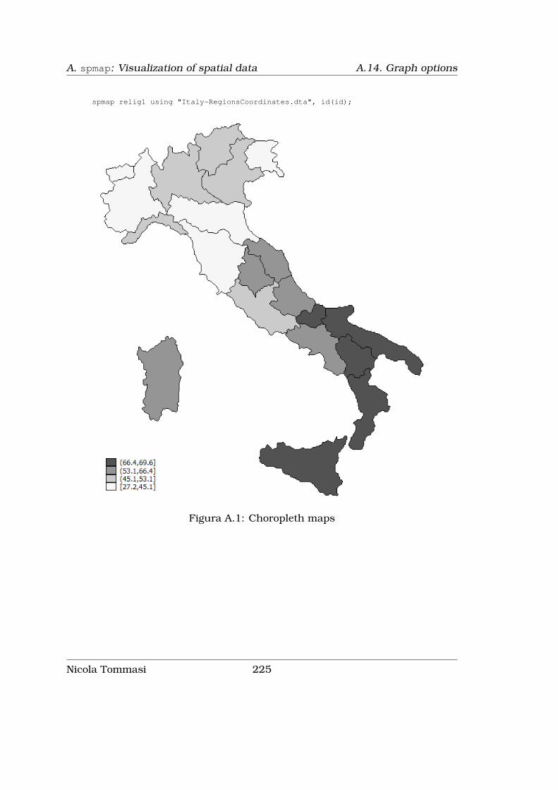
A. spmap: Visualization of spatial data A.14. Graph options
spmap relig1 using "Italy-RegionsCoordinates.dta", id(id);
Figura A.1: Choropleth maps
Nicola Tommasi 225

A.14. Graph options A. spmap: Visualization of spatial data
spmap relig1 using "Italy-RegionsCoordinates.dta", id(id)title("Pct. Catholics without reservations", size(*0.8))subtitle("Italy, 1994-98" " ", size(*0.8));
Figura A.2: Choropleth maps
226 Nicola Tommasi

A. spmap: Visualization of spatial data A.14. Graph options
spmap relig1 using "Italy-RegionsCoordinates.dta", id(id)title("Pct. Catholics without reservations", size(*0.8))subtitle("Italy, 1994-98" " ", size(*0.8))legstyle(2) legend(region(lcolor(black)));
Figura A.3: Choropleth maps
Nicola Tommasi 227

A.14. Graph options A. spmap: Visualization of spatial data
spmap relig1m using "Italy-RegionsCoordinates.dta", id(id)ndfcolor(red)title("Pct. Catholics without reservations", size(*0.8))subtitle("Italy, 1994-98" " ", size(*0.8))legstyle(2) legend(region(lcolor(black)));
Figura A.4: Choropleth maps
228 Nicola Tommasi
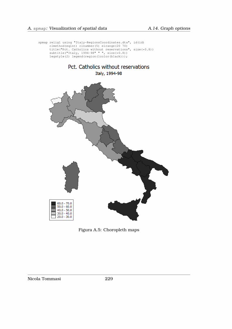
A. spmap: Visualization of spatial data A.14. Graph options
spmap relig1 using "Italy-RegionsCoordinates.dta", id(id)clmethod(eqint) clnumber(5) eirange(20 70)title("Pct. Catholics without reservations", size(*0.8))subtitle("Italy, 1994-98" " ", size(*0.8))legstyle(2) legend(region(lcolor(black)));
Figura A.5: Choropleth maps
Nicola Tommasi 229
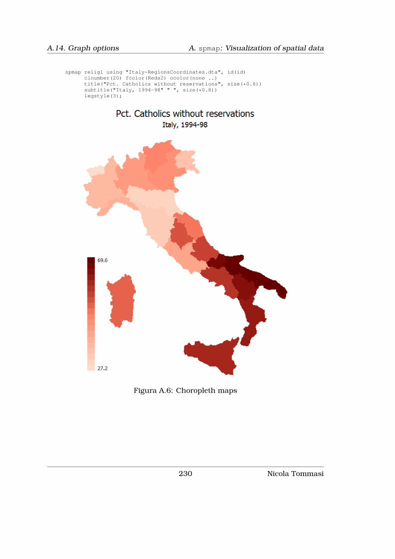
A.14. Graph options A. spmap: Visualization of spatial data
spmap relig1 using "Italy-RegionsCoordinates.dta", id(id)clnumber(20) fcolor(Reds2) ocolor(none ..)title("Pct. Catholics without reservations", size(*0.8))subtitle("Italy, 1994-98" " ", size(*0.8))legstyle(3);
Figura A.6: Choropleth maps
230 Nicola Tommasi

A. spmap: Visualization of spatial data A.14. Graph options
spmap relig1 using "Italy-RegionsCoordinates.dta", id(id)clnumber(20) fcolor(Reds2) ocolor(none ..)title("Pct. Catholics without reservations", size(*0.8))subtitle("Italy, 1994-98" " ", size(*0.8))legstyle(3) legend(ring(1) position(3));
Figura A.7: Choropleth maps
Nicola Tommasi 231

A.14. Graph options A. spmap: Visualization of spatial data
spmap relig1 using "Italy-RegionsCoordinates.dta", id(id)clnumber(20) fcolor(Reds2) ocolor(none ..)title("Pct. Catholics without reservations", size(*0.8))subtitle("Italy, 1994-98" " ", size(*0.8))legstyle(3) legend(ring(1) position(3))plotregion(margin(vlarge));
Figura A.8: Choropleth maps
232 Nicola Tommasi

A. spmap: Visualization of spatial data A.14. Graph options
spmap relig1 using "Italy-RegionsCoordinates.dta", id(id)clnumber(20) fcolor(Reds2) ocolor(none ..)title("Pct. Catholics without reservations", size(*0.8))subtitle("Italy, 1994-98" " ", size(*0.8))legstyle(3) legend(ring(1) position(3))plotregion(icolor(stone)) graphregion(icolor(stone));
Figura A.9: Choropleth maps
Nicola Tommasi 233

A.14. Graph options A. spmap: Visualization of spatial data
spmap relig1 using "Italy-RegionsCoordinates.dta", id(id)clnumber(20) fcolor(Greens2) ocolor(white ..) osize(medthin ..)title("Pct. Catholics without reservations", size(*0.8))subtitle("Italy, 1994-98" " ", size(*0.8))legstyle(3) legend(ring(1) position(3))plotregion(icolor(stone)) graphregion(icolor(stone));
Figura A.10: Choropleth maps
234 Nicola Tommasi

A. spmap: Visualization of spatial data A.14. Graph options
spmap relig1 using "Italy-RegionsCoordinates.dta", id(id)clnumber(20) fcolor(Greens2) ocolor(white ..) osize(thin ..)title("Pct. Catholics without reservations", size(*0.8))subtitle("Italy, 1994-98" " ", size(*0.8))legstyle(3) legend(ring(1) position(3))plotregion(icolor(stone)) graphregion(icolor(stone))polygon(data("Italy-Highlights.dta") ocolor(white)osize(medthick));
Figura A.11: Choropleth maps
Nicola Tommasi 235

A.14. Graph options A. spmap: Visualization of spatial data
spmap relig1 using "Italy-RegionsCoordinates.dta", id(id)clnumber(20) fcolor(Greens2) ocolor(white ..) osize(medthin ..)title("Pct. Catholics without reservations", size(*0.8))subtitle("Italy, 1994-98" " ", size(*0.8))legstyle(3) legend(ring(1) position(3))plotregion(icolor(stone)) graphregion(icolor(stone))scalebar(units(500) scale(1/1000) xpos(-100) label(Kilometers));
Figura A.12: Choropleth maps
236 Nicola Tommasi

A. spmap: Visualization of spatial data A.14. Graph options
spmap using "Italy-OutlineCoordinates.dta", id(id)title("Pct. Catholics without reservations", size(*0.8))subtitle("Italy, 1994-98" " ", size(*0.8))point(data("Italy-RegionsData.dta") xcoord(xcoord)ycoord(ycoord) proportional(relig1) fcolor(red) size(*1.5));
Figura A.13: Proportional symbol maps
Nicola Tommasi 237

A.14. Graph options A. spmap: Visualization of spatial data
spmap using "Italy-OutlineCoordinates.dta", id(id)title("Pct. Catholics without reservations", size(*0.8))subtitle("Italy, 1994-98" " ", size(*0.8))point(data("Italy-RegionsData.dta") xcoord(xcoord)ycoord(ycoord) proportional(relig1) fcolor(red) size(*1.5)shape(s));
Figura A.14: Proportional symbol maps
238 Nicola Tommasi

A. spmap: Visualization of spatial data A.14. Graph options
spmap using "Italy-OutlineCoordinates.dta", id(id)title("Pct. Catholics without reservations", size(*0.8))subtitle("Italy, 1994-98" " ", size(*0.8))point(data("Italy-RegionsData.dta") xcoord(xcoord)ycoord(ycoord) proportional(relig1) fcolor(red)ocolor(white) size(*3))label(data("Italy-RegionsData.dta") xcoord(xcoord)ycoord(ycoord) label(relig1) color(white) size(*0.7));
Figura A.15: Proportional symbol maps
Nicola Tommasi 239

A.14. Graph options A. spmap: Visualization of spatial data
spmap using "Italy-OutlineCoordinates.dta", id(id)title("Pct. Catholics without reservations", size(*0.8))subtitle("Italy, 1994-98" " ", size(*0.8))point(data("Italy-RegionsData.dta") xcoord(xcoord)ycoord(ycoord) deviation(relig1) fcolor(red) dmax(30)legenda(on) leglabel(Deviation from the mean));
Figura A.16: Proportional symbol maps
240 Nicola Tommasi
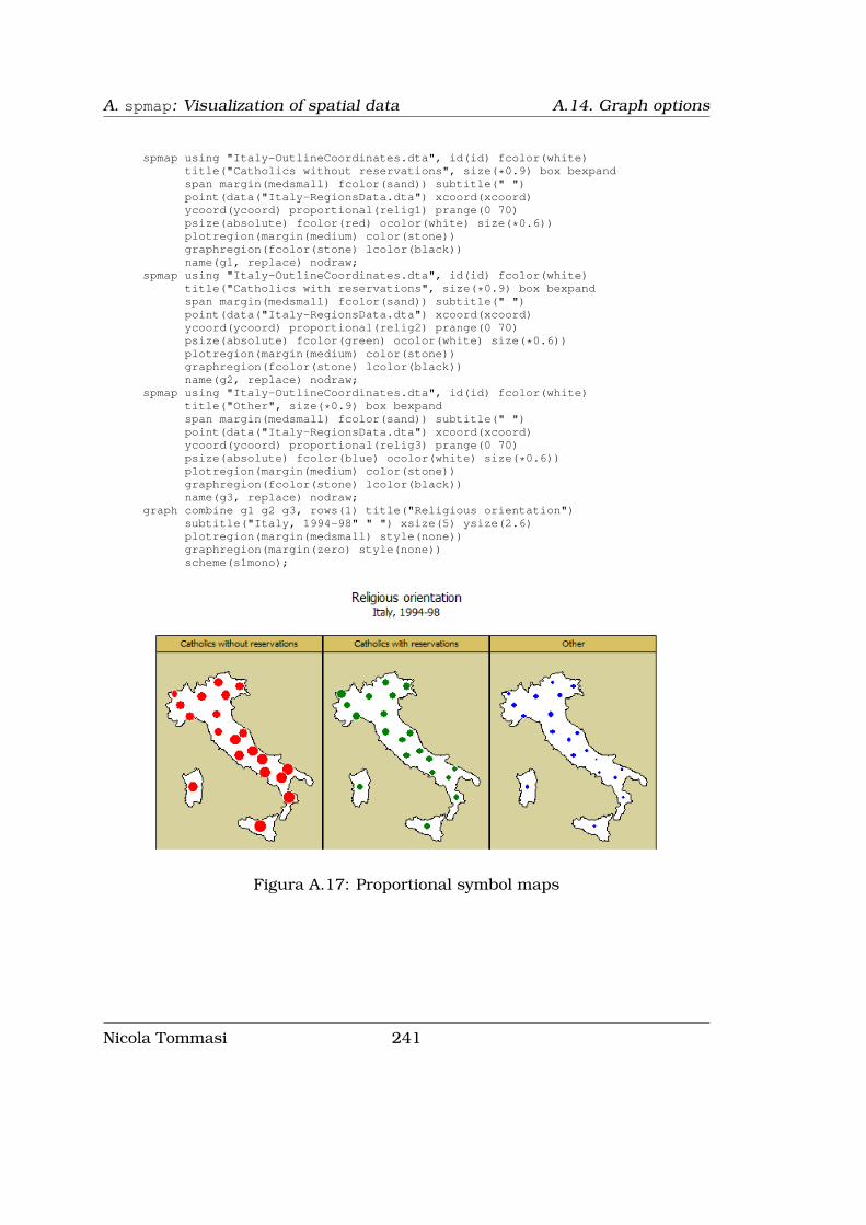
A. spmap: Visualization of spatial data A.14. Graph options
spmap using "Italy-OutlineCoordinates.dta", id(id) fcolor(white)title("Catholics without reservations", size(*0.9) box bexpandspan margin(medsmall) fcolor(sand)) subtitle(" ")point(data("Italy-RegionsData.dta") xcoord(xcoord)ycoord(ycoord) proportional(relig1) prange(0 70)psize(absolute) fcolor(red) ocolor(white) size(*0.6))plotregion(margin(medium) color(stone))graphregion(fcolor(stone) lcolor(black))name(g1, replace) nodraw;
spmap using "Italy-OutlineCoordinates.dta", id(id) fcolor(white)title("Catholics with reservations", size(*0.9) box bexpandspan margin(medsmall) fcolor(sand)) subtitle(" ")point(data("Italy-RegionsData.dta") xcoord(xcoord)ycoord(ycoord) proportional(relig2) prange(0 70)psize(absolute) fcolor(green) ocolor(white) size(*0.6))plotregion(margin(medium) color(stone))graphregion(fcolor(stone) lcolor(black))name(g2, replace) nodraw;
spmap using "Italy-OutlineCoordinates.dta", id(id) fcolor(white)title("Other", size(*0.9) box bexpandspan margin(medsmall) fcolor(sand)) subtitle(" ")point(data("Italy-RegionsData.dta") xcoord(xcoord)ycoord(ycoord) proportional(relig3) prange(0 70)psize(absolute) fcolor(blue) ocolor(white) size(*0.6))plotregion(margin(medium) color(stone))graphregion(fcolor(stone) lcolor(black))name(g3, replace) nodraw;
graph combine g1 g2 g3, rows(1) title("Religious orientation")subtitle("Italy, 1994-98" " ") xsize(5) ysize(2.6)plotregion(margin(medsmall) style(none))graphregion(margin(zero) style(none))scheme(s1mono);
Figura A.17: Proportional symbol maps
Nicola Tommasi 241

A.14. Graph options A. spmap: Visualization of spatial data
spmap using "Italy-RegionsCoordinates.dta", id(id) fcolor(stone)title("Pct. Catholics without reservations", size(*0.8))subtitle("Italy, 1994-98" " ", size(*0.8))diagram(variable(relig1) range(0 100) refweight(pop98)xcoord(xcoord) ycoord(ycoord) fcolor(red));
Figura A.18: Other maps
242 Nicola Tommasi

A. spmap: Visualization of spatial data A.14. Graph options
spmap using "Italy-RegionsCoordinates.dta", id(id) fcolor(stone)diagram(variable(relig1 relig2 relig3) proportional(fortell)xcoord(xcoord) ycoord(ycoord) legenda(on))legend(title("Religious orientation", size(*0.5) bexpandjustification(left)))note(" ""NOTE: Chart size proportional to number of fortune tellersper million population",
size(*0.75));
Figura A.19: Other maps
Nicola Tommasi 243

A.14. Graph options A. spmap: Visualization of spatial data
spmap relig1 using "Italy-RegionsCoordinates.dta", id(id)clmethod(stdev) clnumber(5)title("Pct. Catholics without reservations", size(*0.8))subtitle("Italy, 1994-98" " ", size(*0.8)) area(pop98)note(" ""NOTE: Region size proportional to population", size(*0.75));
Figura A.20: Other maps
244 Nicola Tommasi

A. spmap: Visualization of spatial data A.14. Graph options
spmap relig1 using "Italy-RegionsCoordinates.dta", id(id)clmethod(stdev) clnumber(5)title("Pct. Catholics without reservations", size(*0.8))subtitle("Italy, 1994-98" " ", size(*0.8)) area(pop98)map("Italy-OutlineCoordinates.dta") mfcolor(stone)note(" ""NOTE: Region size proportional to population", size(*0.75));
Figura A.21: Other maps
Nicola Tommasi 245

A.14. Graph options A. spmap: Visualization of spatial data
spmap using "Italy-OutlineCoordinates.dta", id(id) fc(bluishgray)ocolor(none)title("Provincial capitals" " ", size(*0.9) color(white))point(data("Italy-Capitals.dta") xcoord(xcoord)ycoord(ycoord) fcolor(emerald))plotregion(margin(medium) icolor(dknavy) color(dknavy))graphregion(icolor(dknavy) color(dknavy));
Figura A.22: Other maps
246 Nicola Tommasi

A. spmap: Visualization of spatial data A.14. Graph options
spmap using "Italy-OutlineCoordinates.dta", id(id) fc(bluishgray)ocolor(none)title("Provincial capitals" " ", size(*0.9) color(white))point(data("Italy-Capitals.dta") xcoord(xcoord)ycoord(ycoord) by(size) fcolor(orange red maroon) shape(s ..)legenda(on))legend(title("Population 1998", size(*0.5) bexpandjustification(left)) region(lcolor(black) fcolor(white))position(2))plotregion(margin(medium) icolor(dknavy) color(dknavy))graphregion(icolor(dknavy) color(dknavy));
Figura A.23: Other maps
Nicola Tommasi 247
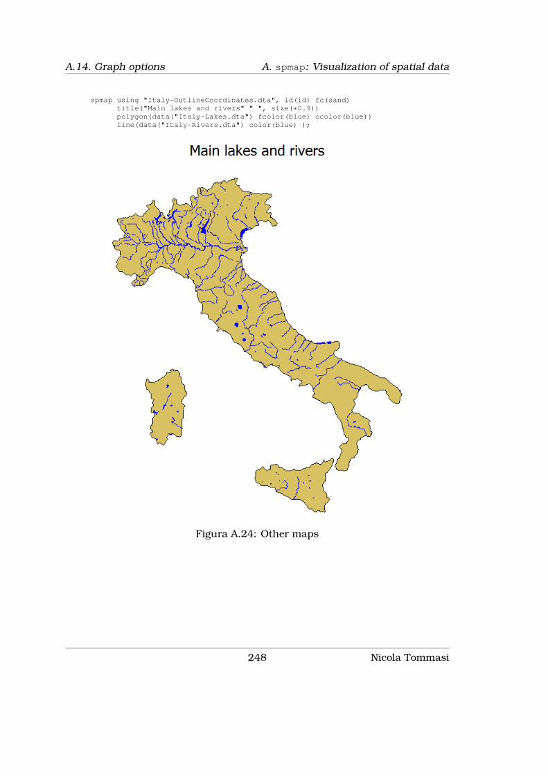
A.14. Graph options A. spmap: Visualization of spatial data
spmap using "Italy-OutlineCoordinates.dta", id(id) fc(sand)title("Main lakes and rivers" " ", size(*0.9))polygon(data("Italy-Lakes.dta") fcolor(blue) ocolor(blue))line(data("Italy-Rivers.dta") color(blue) );
Figura A.24: Other maps
248 Nicola Tommasi

A. spmap: Visualization of spatial data A.14. Graph options
use "Italy-RegionsData.dta", clear;spmap relig1 using "Italy-RegionsCoordinates.dta" if zone==1,
id(id) fcolor(Blues2) ocolor(white ..) osize(medthin ..)title("Pct. Catholics without reservations", size(*0.8))subtitle("Northern Italy, 1994-98" " ", size(*0.8))polygon(data("Italy-OutlineCoordinates.dta") fcolor(gs12)ocolor(white) osize(medthin)) polyfirst;
Figura A.25: Other maps
Nicola Tommasi 249

A.14. Graph options A. spmap: Visualization of spatial data
use "Italy-OutlineData.dta", clear;spmap using "Italy-OutlineCoordinates.dta", id(id) fc(sand)
title("Main lakes and rivers" " ", size(*0.9))polygon(data("Italy-Lakes.dta") fcolor(blue) ocolor(blue))line(data("Italy-Rivers.dta") color(blue) )freestyle aspect(1.4) xlab(400000 900000 1400000, grid);
Figura A.26: Other maps
250 Nicola Tommasi

A. spmap: Visualization of spatial data A.15. Acknowledgments
A.15 Acknowledgments
I wish to thank Nick Cox, Ian Evans, and Vince Wiggins for helping set up tmap(Pisati 2004), the predecessor of spmap. I also thank Kevin Crow, Bill Gould,Friedrich Huebler, and Scott Merryman for promoting tmap by making avail-able to the Stata community several helpful resources related to the program.The development of spmap benefitted from suggestions by Joao Pedro Azevedo,Kit Baum, Daniele Checchi, Kevin Crow, David Drukker, Friedrich Huebler,Laszlo Kardos, Ulrich Kohler, Scott Merryman, Derek Wagner, the participantsin the 1st Italian Stata Users Group Meeting, and the participants in the 3rdGerman Stata Users Group Meeting: many thanks to all of them.
Nicola Tommasi 251

A.15. Acknowledgments A. spmap: Visualization of spatial data
252 Nicola Tommasi

Bibliografia
[1] Armstrong, M.P., Xiao, N. and D.A. Bennett. 2003. Using genetic algo-rithms to create multicriteria class intervals for choropleth maps. Annalsof the Association of American Geographers 93: 595-623.
[2] Brewer, C.A. 1999. Color use guidelines for data representation. Pro-ceedings of the Section on Statistical Graphics, American StatisticalAssociation. Alexandria VA, 55-60.
[3] Brewer, C.A., Hatchard, G.W. and M.A. Harrower. 2003. ColorBrewer inprint: A catalog of color schemes for maps. Cartography and GeographicInformation Science 52: 5-32.
[4] Cleveland, W.S. 1994. The Elements of Graphing Data. Summit: HobartPress.
[5] Cleveland, W.S. and R. McGill. 1984. Graphical perception: Theory, ex-perimentation, and application to the development of graphical methods.Journal of the American Statistical Association 79: 531-554.
[6] Evans, I.S. 1977. The selection of class intervals. Transactions of theInstitute of British Geographers 2: 98-124.
[7] Olson, J.M. 1976. Noncontiguous area cartograms. The ProfessionalGeographer 28: 371-380.
[8] Pisati, M. 2004. Simple thematic mapping. The Stata Journal 4: 361-378.
[9] Slocum, T.A., McMaster, R.B., Kessler, F.C and H.H. Howard. 2005. The-matic Cartography and Geographic Visualization. 2nd ed. Upper SaddleRiver: Pearson Prentice Hall.
253


Appendice B
Lista pacchetti aggiuntivi
. ssc whatshot, n(.)
Packages at SSC
Jul2008Rank # hits Package Author(s)----------------------------------------------------------------------
1 1519.1 outreg2 Roy Wada2 852.6 ivreg2 Mark E Schaffer, Christopher F Baum,
Steven Stillman3 821.5 estout Ben Jann4 763.0 outreg John Luke Gallup5 748.8 psmatch2 Barbara Sianesi, Edwin Leuven6 744.7 xtabond2 David Roodman7 457.0 gllamm Sophia Rabe-Hesketh8 393.2 xtivreg2 Mark E Schaffer9 386.7 overid Steven Stillman, Christopher F Baum,
Vince Wiggins, Mark E Schaffer10 350.3 shp2dta Kevin Crow11 335.0 tabout Ian Watson12 323.8 spmap Maurizio Pisati13 308.0 ranktest Frank Kleibergen, Mark E Schaffer14 282.1 metan Ross Harris, Jon Deeks, Mike Bradburn,
Doug Altman, Roger Harbord, ThomasSteichen, Jonathan Sterne
15 282.0 mif2dta Maurizio Pisati16 258.3 xml_tab Michael Lokshin, Zurab Sajaia17 253.7 oaxaca Ben Jann18 210.5 cmp David Roodman19 205.7 whitetst Christopher F Baum, Nicholas J. Cox20 193.2 ineqdeco Stephen P. Jenkins21 190.7 ivendog Mark E Schaffer, Steven Stillman,
Christopher F Baum22 190.4 ice Patrick Royston23 189.8 ginidesc Roger Aliaga, Silvia Montoya24 184.5 egenmore Nicholas J. Cox25 183.3 mfx2 Richard Williams26 183.0 mmerge Jeroen Weesie27 181.7 winsor Nicholas J. Cox28 177.0 ipshin Christopher F Baum, Fabian Bornhorst29 172.2 hprescott Christopher F Baum30 169.7 elapse Fred Zimmerman31 168.8 outtable Joao Pedro Azevedo, Christopher F Baum32 166.7 levinlin Fabian Bornhorst, Christopher F Baum
255

B. Lista pacchetti aggiuntivi
33 162.5 outtex Antoine Terracol34 158.3 xtwest Joakim Westerlund, Damiaan Persyn35 142.3 xtoverid Mark E Schaffer, Steven Stillman36 141.0 abar David Roodman37 141.0 fitstat J. Scott Long, Jeremy Freese38 133.8 tmap Maurizio Pisati39 128.3 moremata Ben Jann40 126.0 mim John C. Galati, John B. Carlin, Patrick
Royston41 122.7 tsspell Nicholas J. Cox42 120.7 fre Ben Jann43 120.0 xtfisher Scott Merryman44 117.3 tableplot Nicholas J. Cox45 114.0 margeff Tamas Bartus46 114.0 xttest2 Christopher F Baum47 110.0 zandrews Christopher F Baum48 109.0 ftest Maarten L. Buis49 107.2 metareg Roger Harbord, Thomas Steichen50 106.7 unique Tony Brady51 105.7 parmest Roger Newson52 105.3 xttest3 Christopher F Baum53 104.7 fairlie Ben Jann54 102.3 gologit2 Richard Williams55 101.7 bpagan Christopher F Baum, Vince Wiggins56 101.5 sutex Antoine Terracol57 101.0 ghk2 David Roodman58 100.3 latab Ian Watson59 100.0 rd Austin Nichols60 99.0 tsmktim Christopher F Baum, Vince Wiggins61 96.3 corrtex Nicolas Couderc62 96.2 xtpmg Mark W. Frank, Edward F. Blackburne III63 95.0 mvsumm Nicholas J. Cox, Christopher F Baum64 93.8 ineqdec0 Stephen P. Jenkins65 93.7 batplot Adrian Mander66 93.7 shortdir Dan Blanchette67 92.7 nnmatch David M. Drukker, Alberto Abadie, Jane
Leber Herr, Guido W. Imbens68 90.0 confirmdir Dan Blanchette69 89.8 tmpdir Dan Blanchette70 89.7 tab3way Philip Ryan71 89.3 stpiece Jesper B. Sorensen72 88.9 somersd Roger Newson73 88.3 statsmat Nicholas J. Cox, Christopher F Baum74 88.0 hadrilm Christopher F Baum75 88.0 rollreg Christopher F Baum76 85.7 madfuller Christopher F Baum77 84.0 metabias Thomas Steichen78 83.7 xtfmb Daniel Hoechle79 83.0 ivreg28 Mark E Schaffer, Steven Stillman,
Christopher F Baum80 83.0 kernreg2 Makoto Shimizu, Isaias H.
Salgado-Ugarte, Nicholas J. Cox, ToruTaniuchi
81 82.3 omodel Rory Wolfe82 82.2 kdens2 Christopher F Baum83 81.5 oaxaca8 Ben Jann84 81.5 grqreg Joao Pedro Azevedo85 81.0 tabplot Nicholas J. Cox86 80.7 _gwtmean David Kantor87 78.8 surface Adrian Mander88 78.7 inequal7 Philippe Van Kerm89 78.7 johans Ken Heinecke, Charles Morris, Patrick
Joly90 77.7 raschtestv7 Jean-Benoit Hardouin91 77.7 metagraph Adrian Mander
256 Nicola Tommasi
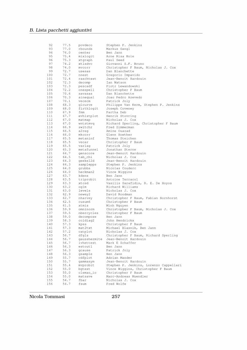
B. Lista pacchetti aggiuntivi
92 77.5 povdeco Stephen P. Jenkins93 77.0 rbounds Markus Gangl94 76.0 center Ben Jann95 75.4 mixlogit Arne Risa Hole96 75.3 xtgraph Paul Seed97 74.2 xtlsdvc Giovanni S.F. Bruno98 74.0 mvcorr Christopher F Baum, Nicholas J. Cox99 72.7 usesas Dan Blanchette100 72.7 nnest Gregorio Impavido101 72.4 raschtest Jean-Benoit Hardouin102 72.3 decomp Ian Watson103 72.3 pescadf Piotr Lewandowski104 72.2 onespell Christopher F Baum105 70.6 savasas Dan Blanchette106 70.3 ainequal Joao Pedro Azevedo107 70.1 vececm Patrick Joly108 68.3 glcurve Philippe Van Kerm, Stephen P. Jenkins109 68.0 firthlogit Joseph Coveney110 67.9 fmm Partha Deb111 67.7 evhistplot Henrik Stovring112 67.0 matmap Nicholas J. Cox113 67.0 wntstmvq Richard Sperling, Christopher F Baum114 66.9 switchr Fred Zimmerman115 66.5 a2reg Amine Ouazad116 66.0 mkcorr Glenn Hoetker117 65.5 metaninf Thomas Steichen118 65.5 vecar Christopher F Baum119 65.5 varlag Patrick Joly120 65.3 metafunnel Jonathan Sterne121 64.7 genscore Jean-Benoit Hardouin122 64.5 tab_chi Nicholas J. Cox123 64.3 geekel2d Jean-Benoit Hardouin124 64.3 samplepps Stephen P. Jenkins125 64.0 grubbs Nicolas Couderc126 64.0 heckman2 Vince Wiggins127 63.7 kdens Ben Jann128 63.5 triprobit Antoine Terracol129 63.3 xtcsd Vasilis Sarafidis, R. E. De Hoyos130 63.2 oglm Richard Williams131 63.0 levels Nicholas J. Cox132 62.9 newey2 David Roodman133 62.7 nharvey Christopher F Baum, Fabian Bornhorst134 62.5 cusum6 Christopher F Baum135 61.5 xtmis Minh Nguyen136 59.9 omninorm Christopher F Baum, Nicholas J. Cox137 59.5 nbercycles Christopher F Baum138 59.0 decompose Ben Jann139 58.3 coldiag2 John Hendrickx140 57.3 kpss Christopher F Baum141 57.3 mat2txt Michael Blasnik, Ben Jann142 57.2 catplot Nicholas J. Cox143 56.7 dfgls Christopher F Baum, Richard Sperling144 56.7 gausshermite Jean-Benoit Hardouin145 56.7 ivhettest Mark E Schaffer146 56.3 estout1 Ben Jann147 56.3 gcause Patrick Joly148 56.3 gsample Ben Jann149 55.7 cdfplot Adrian Mander150 55.7 gammasym Jean-Benoit Hardouin151 55.4 mvprobit Stephen P. Jenkins, Lorenzo Cappellari152 55.0 bgtest Vince Wiggins, Christopher F Baum153 55.0 clemao_io Christopher F Baum154 55.0 matsave Marc-Andreas Muendler155 54.7 fbar Nicholas J. Cox156 54.7 fsum Fred Wolfe
Nicola Tommasi 257

B. Lista pacchetti aggiuntivi
157 54.7 pgmhaz8 Stephen P. Jenkins158 54.0 dtobit2 Vince Wiggins159 54.0 ptrend Patrick Royston160 53.7 byvar Patrick Royston161 53.7 dfl Joao Pedro Azevedo162 53.3 anogi Ben Jann163 53.3 distinct Gary Longton, Nicholas J. Cox164 53.3 kernreg1 Isaias H. Salgado-Ugarte, Toru
Taniuchi, Makoto Shimizu, Xavi Ramos165 53.3 panelunit Christopher F Baum166 53.3 panelauto Christopher F Baum167 53.1 qsim Fred Wolfe168 53.0 dups Nicholas J. Cox, Thomas Steichen169 52.8 todate Nicholas J. Cox170 52.8 vecar6 Patrick Joly, Christopher F Baum171 52.4 mylabels Nicholas J. Cox, Scott Merryman172 52.3 stcompet Enzo Coviello173 52.3 dmexogxt Christopher F Baum, Steven Stillman174 52.3 makematrix Nicholas J. Cox175 52.3 renames Nicholas J. Cox176 52.2 ivpois Austin Nichols177 51.3 eclplot Roger Newson178 51.2 ivprob-ivtobit6 Joseph Harkness179 50.7 bugsdat Adrian Mander180 50.7 poverty Philippe Van Kerm181 50.3 sumdist Stephen P. Jenkins182 50.1 strsrcs C. P. Nelson183 50.0 hausman Jeroen Weesie184 49.6 desmat John Hendrickx185 49.3 fastgini Zurab Sajaia186 49.3 glst Sander Greenland, Nicola Orsini, Rino
Bellocco187 49.3 hshaz Stephen P. Jenkins188 49.3 outsum Kerry L. Papps189 49.3 tabexport Nicholas J. Cox190 48.7 semean Christopher F Baum191 48.5 ralloc Philip Ryan192 48.3 goprobit Stefan Boes193 48.3 heterogi Matteo Bottai, Julian Higgins, Nicola
Orsini, Iain Buchan194 48.3 ivreset Mark E Schaffer195 48.0 adoedit Dan Blanchette196 48.0 metatrim Thomas Steichen197 47.8 movestay Zurab Sajaia, Michael Lokshin198 47.7 stkerhaz Enzo Coviello199 47.3 sensatt Tommaso Nannicini200 47.0 jb6 J. Sky David, Gregorio Impavido201 47.0 xtpqml Tim Simcoe202 46.3 pantest2 Nicholas Oulton203 46.0 est2tex Marc-Andreas Muendler204 45.7 meoprobit Thomas Cornelissen205 45.3 reformat Tony Brady206 45.0 bic Paul Millar207 44.7 concord Thomas Steichen, Nicholas J. Cox208 44.0 bitobit Daniel Lawson209 43.3 rc_spline William D. Dupont, W. Dale Plummer, Jr.210 43.3 xtscc Daniel Hoechle211 43.1 bioprobit Zurab Sajaia212 43.0 charlson Vicki Stagg213 42.7 tabstatmat Austin Nichols214 42.3 meta_lr Aijing Shang215 42.3 probexog-tobexog Christopher F Baum216 42.1 sq Magdalena Luniak, Ulrich Kohler,
Christian Brzinsky-Fay217 42.0 duncan Ben Jann
258 Nicola Tommasi

B. Lista pacchetti aggiuntivi
218 42.0 ivgmm0 David M. Drukker, Christopher F Baum219 42.0 keyplot Nicholas J. Cox220 42.0 mcenter Jeffrey S. Simons221 42.0 tablemat Amadou Bassirou Diallo222 41.8 triplot Nicholas J. Cox223 41.7 coldiag Joseph Harkness224 41.3 catenate Nicholas J. Cox225 41.3 mktab Nick Winter226 41.3 parplot Nicholas J. Cox227 41.2 spsurv Stephen P. Jenkins228 41.0 labutil Nicholas J. Cox229 41.0 descogini Alejandro Lopez-Feldman230 41.0 kr20 Herve M. Caci231 41.0 metagen Pantelis Bagos232 40.7 matvsort Nicholas J. Cox233 40.7 ssm Sophia Rabe-Hesketh, Alfonso Miranda234 40.5 hotdeck David Clayton, Adrian Mander235 40.5 iia Jeroen Weesie236 40.3 dolog Roger Newson237 40.3 markov Nicholas J. Cox238 40.3 valuesof Ben Jann239 40.3 varlab Patrick Joly240 40.2 nmissing Nicholas J. Cox241 40.1 cart Wim van Putten242 40.0 pcorr2 Richard Williams243 39.7 arimafit Christopher F Baum244 39.7 sxpose Nicholas J. Cox245 39.7 tolower Nicholas J. Cox246 39.4 dologx Roger Newson247 39.3 crtest Joao Pedro Azevedo248 39.3 lomackinlay Christopher F Baum249 39.3 metandi Roger Harbord250 39.3 egen_inequal Michael Lokshin, Zurab Sajaia251 39.0 gdecomp Tamas Bartus252 39.0 hansen2 Nicholas J. Cox253 39.0 hireg Paul H. Bern254 39.0 jb Gregorio Impavido, J. Sky David255 38.7 alorenz Samuel Franco, Joao Pedro Azevedo256 38.7 ivvif David Roodman257 38.7 nearmrg Michael Blasnik, Katherine Smith258 38.7 svygei_svyatk Stephen P. Jenkins, Martin Biewen259 38.5 collapseunique David Kantor260 38.3 kwallis2 Herve M. Caci261 38.3 mlcoint Ken Heinecke262 38.3 predxcat Joanne M. Garrett263 38.3 radar Adrian Mander264 38.0 historaj Rajesh Tharyan265 38.0 ipf Adrian Mander266 38.0 stcmd Roger Newson267 37.8 regoprob Stefan Boes268 37.7 changemean Samuel Franco, Joao Pedro Azevedo269 37.7 tscollap Christopher F Baum270 37.3 dmariano Christopher F Baum271 37.3 durbinh Christopher F Baum, Vince Wiggins272 37.0 corrtable Nicholas J. Cox273 37.0 msp Jean-Benoit Hardouin274 36.7 bcoeff Nicholas J. Cox, Zhiqiang Wang275 36.7 cf3 Thomas Steichen276 36.7 hbar Nicholas J. Cox277 36.7 pyramid Jens M. Lauritsen278 36.7 sampsi_mcc Adrian Mander279 36.5 denton Christopher F Baum280 36.0 hplot Nicholas J. Cox281 36.0 lookfor_all Michael Lokshin, Zurab Sajaia282 36.0 lrplot Jan Brogger
Nicola Tommasi 259

B. Lista pacchetti aggiuntivi
283 36.0 vioplot Nick Winter284 35.7 apoverty Joao Pedro Azevedo285 35.7 lambda Nicholas J. Cox286 35.7 predxcon Joanne M. Garrett287 35.7 quantiles Rafael Guerreiro Osorio288 35.7 sf36 Philip Ryan289 35.5 bspline Roger Newson290 35.4 mahapick David Kantor291 35.3 dummieslab Nicholas J. Cox, Philippe Van Kerm292 35.3 xttrans2 Nicholas J. Cox293 35.0 extremes Nicholas J. Cox294 35.0 tab2way Philip Ryan295 34.7 factortest Joao Pedro Azevedo296 34.7 inequal2 Philippe Van Kerm297 34.7 locpr Austin Nichols298 34.3 maketex Antoine Terracol299 34.3 matwrite Andrew Shephard300 34.3 white Jeroen Weesie301 34.3 wtp Arne Risa Hole302 34.3 xtmrho Lars E. Kroll303 34.3 seqlogit Maarten L. Buis304 34.1 stcoxgof Enzo Coviello305 34.0 ldecomp Maarten L. Buis306 34.0 mca Philippe Van Kerm307 33.8 avplot3 Christopher F Baum308 33.7 distrate Enzo Coviello309 33.7 dotex Roger Newson310 33.7 factext Roger Newson311 33.7 inteff3 Katja Sonderhof, Thomas Cornelissen312 33.7 samplesize Adrian Mander313 33.7 smileplot Roger Newson314 33.6 mvtobit Mikkel Barslund315 33.5 log2html Nicholas J. Cox, Bill Rising,
Christopher F Baum316 33.3 ordplot Nicholas J. Cox317 33.3 spell Richard Goldstein, Nicholas J. Cox318 33.0 fracirf Christopher F Baum319 33.0 groups Nicholas J. Cox320 33.0 ineqfac Stephen P. Jenkins321 32.8 midas Ben Dwamena322 32.7 svytabs Michael Blasnik323 32.3 corrtab Fred Wolfe324 32.3 devcon Ben Jann325 32.3 qic James Cui326 32.0 hegy4 Christopher F Baum, Richard Sperling327 32.0 mvsampsi David E. Moore328 32.0 rocss Nicola Orsini, Matteo Bottai329 31.8 bking Martha Lopez, Christopher F Baum330 31.7 centcalc Eileen Wright, Patrick Royston331 31.7 eret2 Ben Jann332 31.7 scores Dirk Enzmann333 31.7 svylorenz Stephen P. Jenkins334 31.5 powerq Tiago V Pereira, Nikolaos A Patsopoulos335 31.5 qcount Alfonso Miranda336 31.3 descsave Roger Newson337 31.0 jmpierce Ben Jann338 31.0 listtex Roger Newson339 30.8 hlm Sean F. Reardon340 30.8 hnblogit Joseph Hilbe341 30.3 hplogit Joseph Hilbe342 30.3 xsampsi Jan Brogger343 30.2 mgof Ben Jann344 30.0 apc Yang Yang, Sam Schulhofer-Wohl345 30.0 dummies Nicholas J. Cox346 30.0 genass Neil Shephard
260 Nicola Tommasi

B. Lista pacchetti aggiuntivi
347 30.0 ineq Nicholas J. Cox348 30.0 intext Roger Newson349 30.0 scat3 Nicholas J. Cox350 30.0 svyselmlog R. E. De Hoyos351 30.0 tabhbar Nicholas J. Cox352 30.0 xtile2 Zhiqiang Wang353 29.7 cihplot Nicholas J. Cox354 29.7 dmerge Fred Wolfe355 29.7 grfreq Jan Brogger356 29.7 tsgraph Nicholas J. Cox, Christopher F Baum357 29.6 rrlogit Ben Jann358 29.3 cltest Jeph Herrin359 29.3 concindc Zhuo (Adam) Chen360 29.3 oddsrisk Joseph Hilbe361 29.3 probitiv Jonah B. Gelbach362 29.3 vincenty Austin Nichols363 29.3 spautoc Nicholas J. Cox364 29.0 lincomest Roger Newson365 28.7 ciplot Nicholas J. Cox366 28.7 estsave Michael Blasnik367 28.5 _peers Amine Ouazad368 28.3 armadiag Sune Karlsson369 28.3 swboot Joanne M. Garrett370 28.0 imputeitems Jean-Benoit Hardouin371 27.7 archlm Vince Wiggins, Christopher F Baum372 27.7 bigtab Paul H. Bern373 27.7 eba Gregorio Impavido374 27.7 lognfit Stephen P. Jenkins375 27.7 reclink Michael Blasnik376 27.3 cfitzrw Christopher F Baum, Martha Lopez377 27.3 cndnmb3 Michael Blasnik378 27.3 diagtest Aurelio Tobias379 27.3 idonepsu Joshua H. Sarver380 27.3 imputerasch Jean-Benoit Hardouin381 27.3 _gsoundex Michael Blasnik382 27.1 lrutil Jan Brogger383 27.0 clorenz Araar Abdelkrim384 27.0 mvsamp1i David E. Moore385 27.0 xtpattern Nicholas J. Cox386 26.9 hcavar Jean-Benoit Hardouin387 26.8 ocratio Rory Wolfe388 26.7 pre Paul Millar389 26.3 matsort Paul Millar390 26.3 mulogit Leif E. Peterson391 26.3 shapley Stanislav Kolenikov392 26.2 oprobpr Nick Winter393 26.0 bicdrop1 Paul Millar394 26.0 cipolate Nicholas J. Cox395 26.0 etime Dan Blanchette396 26.0 lincheck Alex Gamma397 26.0 overlay Adrian Mander398 26.0 sizefx Matthew Openshaw399 25.7 addnotes Jeff Arnold400 25.7 countmatch Nicholas J. Cox401 25.7 diagt Paul Seed402 25.7 sampsi_rho Adrian Mander403 25.7 simirt Jean-Benoit Hardouin404 25.7 xtarsim Giovanni S.F. Bruno405 25.5 tabhplot Nicholas J. Cox406 25.3 asciiplot Svend Juul, Nicholas J. Cox, Michael
Blasnik407 25.3 chiplot Thomas Steichen408 25.3 collapse2 David Roodman409 25.3 gphudak Vince Wiggins, Christopher F Baum410 25.3 indeplist Maarten L. Buis
Nicola Tommasi 261

B. Lista pacchetti aggiuntivi
411 25.3 xdatelist Roger Newson412 25.3 loevh Jean-Benoit Hardouin413 25.0 gamet Debora Rizzuto, Nicola Orsini, Nicola
Nante414 25.0 imputemok Jean-Benoit Hardouin415 25.0 openall Ari Friedman416 25.0 plotbeta Adrian Mander417 25.0 qll Christopher F Baum418 25.0 sampsi_reg Adrian Mander419 24.9 stpm Patrick Royston420 24.7 betafit Maarten L. Buis, Stephen P. Jenkins,
Nicholas J. Cox421 24.7 clogithet Arne Risa Hole422 24.7 grlogit Jan Brogger423 24.7 nsplit Dan Blanchette424 24.7 savesome Nicholas J. Cox425 24.7 textbarplot Nicholas J. Cox426 24.5 perturb John Hendrickx427 24.3 contour Adrian Mander428 24.3 fastcd Nick Winter429 24.3 fese Austin Nichols430 24.3 fprank Mamoun BenMamoun431 24.3 glcurve7 Philippe Van Kerm, Stephen P. Jenkins432 24.3 icomp Stanislav Kolenikov433 24.3 seq Nicholas J. Cox434 24.3 smhsiao Nick Winter435 24.3 tomata William Gould436 24.3 traces Jean-Benoit Hardouin437 24.0 gologit Vincent Kang Fu438 24.0 hallt-skewt Rajesh Tharyan, Scott Merryman439 24.0 intcens Jamie Griffin440 24.0 rensheet Austin Nichols441 24.0 vmatch Guy D. van Melle442 23.8 estwrite Ben Jann443 23.7 hlp2pdf Christopher F Baum444 23.7 jmpierce2 Ben Jann445 23.7 sparl Nicholas J. Cox446 23.7 xtvc Matteo Bottai, Nicola Orsini447 23.3 cortesti Herve M. Caci448 23.3 domdiag Nicholas J. Cox449 23.3 ivactest Christopher F Baum, Mark E Schaffer450 23.3 rc2 John Hendrickx451 23.3 rcspline Nicholas J. Cox452 23.0 butterworth Christopher F Baum, Martha Lopez453 23.0 isvar Nicholas J. Cox454 23.0 log2do2 Nick Winter455 23.0 lomodrs Tairi Room, Christopher F Baum456 23.0 lrmatx Jan Brogger457 22.8 rnd Joseph Hilbe458 22.7 clv Jean-Benoit Hardouin459 22.7 dsearch Ulrich Kohler460 22.7 lrdrop1 Zhiqiang Wang461 22.7 mlowess Nicholas J. Cox462 22.7 normtest Herve M. Caci463 22.7 sslope Jeffrey S. Simons464 22.7 stak Thomas Steichen465 22.7 svmatf Jan Brogger466 22.7 xrigls Patrick Royston, Eileen Wright467 22.5 tobitiv Jonah B. Gelbach468 22.5 svr Nick Winter469 22.3 blinding Jiefeng Chen470 22.3 ds3 Nicholas J. Cox471 22.3 ghistcum Christopher F Baum, Nicholas J. Cox472 22.3 pairplot Nicholas J. Cox473 22.3 paretofit Stephen P. Jenkins, Philippe Van Kerm
262 Nicola Tommasi
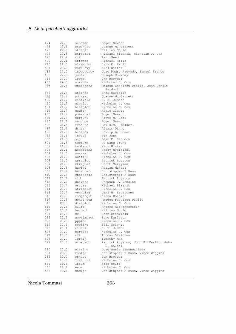
B. Lista pacchetti aggiuntivi
474 22.3 senspec Roger Newson475 22.3 stcoxplt Joanne M. Garrett476 22.3 stcstat William Gould477 22.3 strparse Michael Blasnik, Nicholas J. Cox478 22.2 ci2 Paul Seed479 22.1 effects Michael Hills480 22.0 classplot Lars E. Kroll481 22.0 corr_svy Nick Winter482 22.0 isopoverty Joao Pedro Azevedo, Samuel Franco483 22.0 jonter Joseph Coveney484 22.0 lrchg Jan Brogger485 22.0 moreobs Nicholas J. Cox486 21.8 checkfor2 Amadou Bassirou Diallo, Jean-Benoit
Hardouin487 21.8 starjas Enzo Coviello488 21.7 adjmean Joanne M. Garrett489 21.7 centroid D. H. Judson490 21.7 civplot Nicholas J. Cox491 21.7 histplot Nicholas J. Cox492 21.7 median Mario Cleves493 21.7 powercal Roger Newson494 21.7 sbrowni Herve M. Caci495 21.7 sencode Roger Newson496 21.5 freduse David M. Drukker497 21.4 dthaz Alexis Dinno498 21.3 histbox Philip B. Ender499 21.3 invcdf Ben Jann500 21.3 seg Sean F. Reardon501 21.3 tabform Le Dang Trung502 21.3 tablecol Nick Winter503 21.1 heckprob2 Jerzy Mycielski504 21.0 nearest Nicholas J. Cox505 21.0 outfix2 Nicholas J. Cox506 21.0 xpredict Patrick Royston507 21.0 xtregre2 Scott Merryman508 20.9 hapipf Adrian Mander509 20.7 betacoef Christopher F Baum510 20.7 checkreg3 Christopher F Baum511 20.7 cid Patrick Royston512 20.7 geivars Stephen P. Jenkins513 20.7 mstore Michael Blasnik514 20.7 stripplot Nicholas J. Cox515 20.7 venndiag Jens M. Lauritsen516 20.5 complogit Glenn Hoetker517 20.5 concindex Amadou Bassirou Diallo518 20.3 distplot Nicholas J. Cox519 20.3 ellip Anders Alexandersson520 20.3 hetprob William Gould521 20.3 mcl John Hendrickx522 20.3 newsimpact Sune Karlsson523 20.3 ppplot Nicholas J. Cox524 20.3 reglike Bill Sribney525 20.1 cluster D. H. Judson526 20.0 barplot Nicholas J. Cox527 20.0 cf2 Thomas Steichen528 20.0 lgraph Timothy Mak529 20.0 mimstack Patrick Royston, John B. Carlin, John
C. Galati530 20.0 missing Jose Maria Sanchez Saez531 20.0 roblpr Christopher F Baum, Vince Wiggins532 20.0 sskapp Jan Brogger533 19.9 listutil Nicholas J. Cox534 19.8 lfsum Fred Wolfe535 19.7 ewma Nicholas J. Cox536 19.7 modlpr Christopher F Baum, Vince Wiggins
Nicola Tommasi 263

B. Lista pacchetti aggiuntivi
537 19.7 plotmatrix Adrian Mander538 19.7 recode2 John Hendrickx539 19.7 sphdist Bill Rising540 19.7 survwgt Nick Winter541 19.7 wgttest Ben Jann542 19.7 zipsave Henrik Stovring543 19.5 stpepemori Enzo Coviello544 19.3 hangroot Maarten L. Buis545 19.3 mdensity Nicholas J. Cox546 19.3 povguide David Kantor547 19.3 revrs Kyle C. Longest548 19.3 vallist Patrick Joly549 19.3 xcorplot Nicholas J. Cox, Aurelio Tobias550 19.2 hnbclg Joseph Hilbe551 19.1 modeldiag Nicholas J. Cox552 19.0 cb2html Phil Bardsley553 19.0 cme Sophia Rabe-Hesketh554 19.0 gengroup Jean-Benoit Hardouin555 19.0 soreg Mark Lunt556 19.0 tabmerge Nicholas J. Cox557 19.0 xcontract Roger Newson558 18.9 isko John Hendrickx559 18.7 addtxt Gary Longton560 18.7 episens Sander Greenland, Nicola Orsini, Rino
Bellocco561 18.7 expandby Nicholas J. Cox562 18.7 fitint Neville Verlander, André Charlett563 18.7 metamiss Julian Higgins, Ian White564 18.7 mmsrm Jean-Benoit Hardouin565 18.7 pcorrmat Maarten L. Buis566 18.7 pwcorrs Fred Wolfe567 18.7 rolling2 Christopher F Baum568 18.7 rowranks Nicholas J. Cox569 18.7 rsource Roger Newson570 18.7 ssizebi Abdel G. Babiker571 18.3 acplot Nicholas J. Cox572 18.3 allpossible Nicholas J. Cox573 18.3 ctabstat Nicholas J. Cox574 18.3 dirlist Morten Andersen575 18.3 dissim Nicholas J. Cox576 18.3 kaputil David Harrison577 18.3 matin4-matout4 William Gould, Christopher F Baum578 18.3 paran Alexis Dinno579 18.3 selectvars Nicholas J. Cox580 18.3 split Nicholas J. Cox581 18.3 urcovar Christopher F Baum582 18.3 xcollapse Roger Newson583 18.2 postrcspline Maarten L. Buis584 18.2 tosql Christopher F Baum585 18.1 zip Jesper Sorensen586 18.0 bnormpdf Gary Longton587 18.0 colelms Mark S Pearce, Zhiqiang Wang588 18.0 csjl Jens M. Lauritsen, Thomas Steichen589 18.0 dpredict J. Katriak590 18.0 gpfobl Herve M. Caci591 18.0 longplot Zhiqiang Wang, Nicholas J. Cox592 18.0 mrdum Lee E. Sieswerda593 18.0 relrank Ben Jann594 18.0 richness Thilo Schaefer, Andreas Peichl595 18.0 strgen Nicholas J. Cox596 18.0 taba Nicholas J. Cox597 18.0 wclogit Adrian Mander598 18.0 zinb Jesper Sorensen599 17.8 akdensity Philippe Van Kerm600 17.8 dpplot Nicholas J. Cox
264 Nicola Tommasi
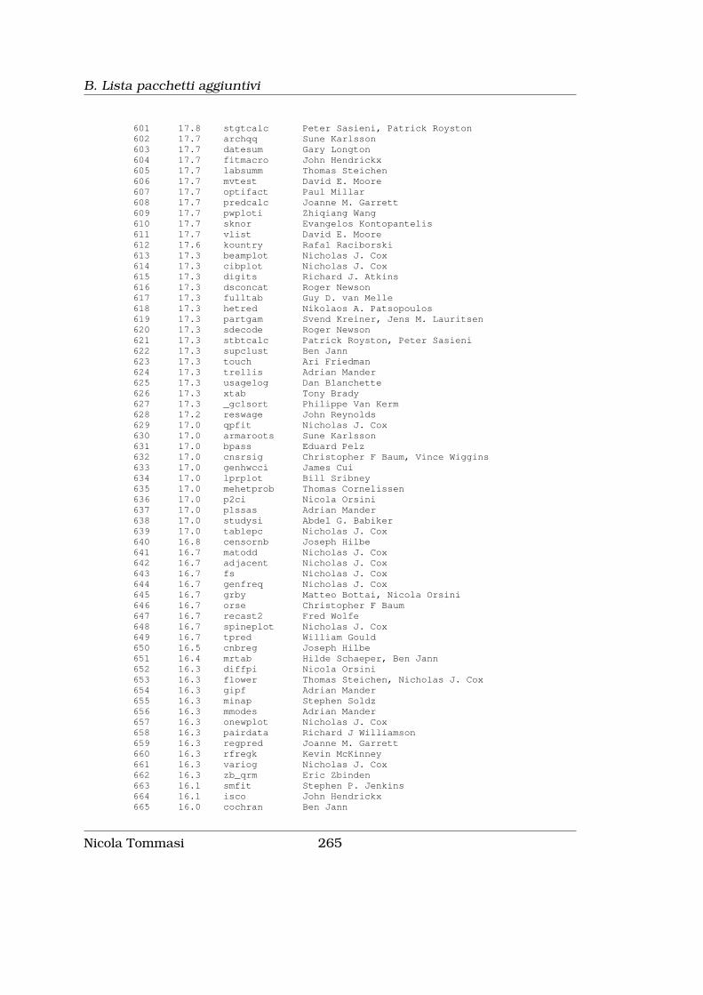
B. Lista pacchetti aggiuntivi
601 17.8 stgtcalc Peter Sasieni, Patrick Royston602 17.7 archqq Sune Karlsson603 17.7 datesum Gary Longton604 17.7 fitmacro John Hendrickx605 17.7 labsumm Thomas Steichen606 17.7 mvtest David E. Moore607 17.7 optifact Paul Millar608 17.7 predcalc Joanne M. Garrett609 17.7 pwploti Zhiqiang Wang610 17.7 sknor Evangelos Kontopantelis611 17.7 vlist David E. Moore612 17.6 kountry Rafal Raciborski613 17.3 beamplot Nicholas J. Cox614 17.3 cibplot Nicholas J. Cox615 17.3 digits Richard J. Atkins616 17.3 dsconcat Roger Newson617 17.3 fulltab Guy D. van Melle618 17.3 hetred Nikolaos A. Patsopoulos619 17.3 partgam Svend Kreiner, Jens M. Lauritsen620 17.3 sdecode Roger Newson621 17.3 stbtcalc Patrick Royston, Peter Sasieni622 17.3 supclust Ben Jann623 17.3 touch Ari Friedman624 17.3 trellis Adrian Mander625 17.3 usagelog Dan Blanchette626 17.3 xtab Tony Brady627 17.3 _gclsort Philippe Van Kerm628 17.2 reswage John Reynolds629 17.0 qpfit Nicholas J. Cox630 17.0 armaroots Sune Karlsson631 17.0 bpass Eduard Pelz632 17.0 cnsrsig Christopher F Baum, Vince Wiggins633 17.0 genhwcci James Cui634 17.0 lprplot Bill Sribney635 17.0 mehetprob Thomas Cornelissen636 17.0 p2ci Nicola Orsini637 17.0 plssas Adrian Mander638 17.0 studysi Abdel G. Babiker639 17.0 tablepc Nicholas J. Cox640 16.8 censornb Joseph Hilbe641 16.7 matodd Nicholas J. Cox642 16.7 adjacent Nicholas J. Cox643 16.7 fs Nicholas J. Cox644 16.7 genfreq Nicholas J. Cox645 16.7 grby Matteo Bottai, Nicola Orsini646 16.7 orse Christopher F Baum647 16.7 recast2 Fred Wolfe648 16.7 spineplot Nicholas J. Cox649 16.7 tpred William Gould650 16.5 cnbreg Joseph Hilbe651 16.4 mrtab Hilde Schaeper, Ben Jann652 16.3 diffpi Nicola Orsini653 16.3 flower Thomas Steichen, Nicholas J. Cox654 16.3 gipf Adrian Mander655 16.3 minap Stephen Soldz656 16.3 mmodes Adrian Mander657 16.3 onewplot Nicholas J. Cox658 16.3 pairdata Richard J Williamson659 16.3 regpred Joanne M. Garrett660 16.3 rfregk Kevin McKinney661 16.3 variog Nicholas J. Cox662 16.3 zb_qrm Eric Zbinden663 16.1 smfit Stephen P. Jenkins664 16.1 isco John Hendrickx665 16.0 cochran Ben Jann
Nicola Tommasi 265

B. Lista pacchetti aggiuntivi
666 16.0 detect Jean-Benoit Hardouin667 16.0 grnote Michael Blasnik668 16.0 gwhet Gregorio Impavido669 16.0 labsort Ross Odell670 16.0 rmanova George M. Hoffman671 16.0 shorth Nicholas J. Cox672 16.0 stbget Nicholas J. Cox673 16.0 tgraph Patrick Royston674 16.0 tknz David C. Elliott675 16.0 univstat Nicholas J. Cox676 15.7 addinby Roger Newson677 15.7 cflpois Jens M. Lauritsen678 15.7 charlist Nicholas J. Cox679 15.7 ciw Nicholas J. Cox680 15.7 datmat Bill Sribney681 15.7 eclpci Nicola Orsini682 15.7 eqprhistogram Nicholas J. Cox683 15.7 finddup Fred Wolfe684 15.7 gentrun Hung-Jen Wang685 15.7 hutchens Stephen P. Jenkins686 15.7 logpred Joanne M. Garrett687 15.7 lstack Nicholas J. Cox688 15.7 medoid D. H. Judson689 15.7 mypkg Nicholas J. Cox690 15.7 outdat Ulrich Kohler691 15.7 pdplot Nicholas J. Cox692 15.7 prepar Laura Gibbons693 15.7 textgph Nick Winter694 15.7 vanelteren Joseph Coveney695 15.7 varcase John R. Gleason696 15.7 vplplot Nicholas J. Cox697 15.5 cpcorr Nicholas J. Cox698 15.5 hpclg Joseph Hilbe699 15.4 invgammafit Nicholas J. Cox, Stephen P. Jenkins700 15.3 ciform Roger Newson701 15.3 cleanlog Lee E. Sieswerda702 15.3 dlist Nicholas J. Cox703 15.3 epsigr Henrik Stovring704 15.3 fndmtch Desmond E. Williams, Nicholas J. Cox705 15.3 hist3 Steffen Kuehnel, Ulrich Kohler706 15.3 ljs Nicholas J. Cox707 15.3 lxpct_2 Margaret M. Weden708 15.3 rgroup Ulrich Kohler709 15.3 torumm Fred Wolfe710 15.3 utest Jo Thori Lind, Halvor Mehlum711 15.3 vallab Nicholas J. Cox712 15.3 wbull Nicholas J. Cox713 15.2 charutil Nicholas J. Cox714 15.2 mkdat Ulrich Kohler715 15.0 alphawgt Ben Jann716 15.0 cpigen Austin Nichols717 15.0 cpr Nicholas J. Cox718 15.0 dfao Richard Sperling719 15.0 ellip7 Anders Alexandersson720 15.0 fixsort Nicholas J. Cox721 15.0 floattolong David Kantor722 15.0 fracdiff Christopher F Baum723 15.0 gmci John Carlin724 15.0 hbox Nicholas J. Cox725 15.0 kdbox Philip B. Ender726 15.0 mapch Ward Vanlaar727 15.0 msplot Nicholas J. Cox728 15.0 pwcorrw Nicholas J. Cox729 15.0 qexp Nicholas J. Cox730 15.0 reorder Nicholas J. Cox
266 Nicola Tommasi

B. Lista pacchetti aggiuntivi
731 15.0 rglm Roger Newson732 15.0 runparscale Laura Gibbons733 15.0 seast Richard Feltbower, Mark S. Pearce734 15.0 smithwelch Ben Jann735 15.0 violin Thomas Steichen736 15.0 vreverse Nicholas J. Cox737 15.0 weibullfit Nicholas J. Cox, Stephen P. Jenkins738 15.0 xfrac Stephen P. Jenkins739 14.9 gzsave Henrik Stovring740 14.8 dirifit Maarten L. Buis, Nicholas J. Cox,
Stephen P. Jenkins741 14.8 groupcl Paulo Guimaraes742 14.7 adjprop Joanne M. Garrett743 14.7 assertky David Kantor744 14.7 benford Nikos Askitas745 14.7 checkrob Mikkel Barslund746 14.7 filei Nicholas J. Cox747 14.7 harmby Roger Newson748 14.7 hcnbreg Joseph Hilbe749 14.7 inccat Roger Newson750 14.7 ivglog Joseph Hilbe751 14.7 kdmany Stanislav Kolenikov752 14.7 nbfit Nicholas J. Cox, Roberto G. Gutierrez753 14.7 nproc Fred Wolfe, Philip Price754 14.7 regaxis Roger Newson755 14.7 sbplot Nicholas J. Cox756 14.7 shuffle Ben Jann757 14.7 skbim Evangelos Kontopantelis758 14.7 spearman2 Christopher F Baum759 14.7 stcascoh Enzo Coviello760 14.7 stquant Enzo Coviello761 14.7 strdate Roger Newson762 14.7 xb2pi Nicola Orsini763 14.5 cpoisson Joseph Hilbe764 14.4 stexpect Enzo Coviello765 14.3 backrasch Jean-Benoit Hardouin766 14.3 carryforward David Kantor767 14.3 chaos Nicholas J. Cox768 14.3 cistat Nicholas J. Cox769 14.3 drarea Adrian Mander770 14.3 feldti Herve M. Caci771 14.3 genvars Jan Brogger772 14.3 gevfit Scott Merryman773 14.3 grand Vince Wiggins774 14.3 ifin Ari Friedman775 14.3 mlogpred Bill Sribney776 14.3 mvsktest Stanislav Kolenikov777 14.3 nbstrat Joseph Hilbe, Roberto Martinez-Espineira778 14.3 progres Philippe van Kerm, Andreas Peichl779 14.3 readlog Jan Brogger780 14.3 tomode Fred Wolfe, Nicholas J. Cox781 14.3 tslist Michael S. Hanson, Christopher F Baum782 14.3 vclose Nicholas J. Cox783 14.3 viewresults Ben Jann784 14.3 _grmedf Stanislav Kolenikov785 14.2 nct Thomas Steichen786 14.2 estparm Roger Newson787 14.2 doub2flt Fred Wolfe788 14.2 glgamma2 Joseph Hilbe789 14.2 hglogit Joseph Hilbe790 14.0 cstable Peter Makary, Gilles Desve791 14.0 difd Laura Gibbons792 14.0 fedit Nicholas J. Cox793 14.0 gammafit Nicholas J. Cox, Stephen P. Jenkins794 14.0 hapblock Adrian Mander
Nicola Tommasi 267

B. Lista pacchetti aggiuntivi
795 14.0 levene Herve M. Caci796 14.0 longch Tony Brady797 14.0 profhap Adrian Mander798 14.0 recap Matthias an der Heiden799 14.0 reshape8 Bill Rising800 14.0 sdline Nicholas J. Cox801 14.0 sratio Mamoun BenMamoun802 14.0 t2way5 Nicholas J. Cox803 14.0 tpvar Nicholas J. Cox804 13.9 circular Nicholas J. Cox805 13.8 fieller Joseph Coveney806 13.8 pbeta Nicholas J. Cox807 13.8 stselpre Enzo Coviello808 13.8 examples Nicholas J. Cox809 13.7 barplot2 Nicholas J. Cox810 13.7 bynote Roger Newson811 13.7 gby Zhiqiang Wang812 13.7 hlpdir Nicholas J. Cox813 13.7 mira Rodrigo Alfaro814 13.7 moments Nicholas J. Cox815 13.7 multibar Fred Wolfe816 13.7 orthog Bill Sribney817 13.7 ovbd Joseph Coveney818 13.7 splitvallabels Ben Jann, Nick Winter819 13.7 tabcount Nicholas J. Cox820 13.7 title Jan Brogger821 13.7 tsplot Aurelio Tobias822 13.7 whotdeck Adrian Mander823 13.6 gb2fit Stephen P. Jenkins824 13.5 avplot2 Nicholas J. Cox825 13.5 sortlistby Ben Jann826 13.4 rfl Dankwart Plattner827 13.3 autolog Ian Watson828 13.3 findval Stanislav Kolenikov829 13.3 firstdigit Nicholas J. Cox830 13.3 gpreset Roger Newson831 13.3 keyby Roger Newson832 13.3 listmiss Paul Millar833 13.3 sbplot5 Nicholas J. Cox834 13.3 skewplot Nicholas J. Cox835 13.3 slideplot Nicholas J. Cox836 13.3 stack William Gould837 13.3 summvl Jeroen Weesie838 13.3 svvarlbl Desmond E. Williams839 13.3 tryem Al Feiveson840 13.3 vartyp Paul H. Bern841 13.3 witch Thomas Steichen842 13.2 gzipuse Nikos Askitas843 13.2 pexp Nicholas J. Cox844 13.1 ellip6 Anders Alexandersson845 13.0 adjust Kenneth Higbee846 13.0 biplot Ulrich Kohler847 13.0 confsvy Zhiqiang Wang848 13.0 factref Roger Newson849 13.0 full_palette Nick Winter850 13.0 grand2 Vince Wiggins851 13.0 graphbinary Adrian Mander852 13.0 istdize Mario Cleves853 13.0 outseries Christopher F Baum854 13.0 ranova Joseph Hilbe855 13.0 safedrop Nicholas J. Cox856 13.0 sbri Nicola Orsini857 13.0 strip P.T.Seed858 13.0 swblock Adrian Mander859 13.0 tuples Nicholas J. Cox
268 Nicola Tommasi
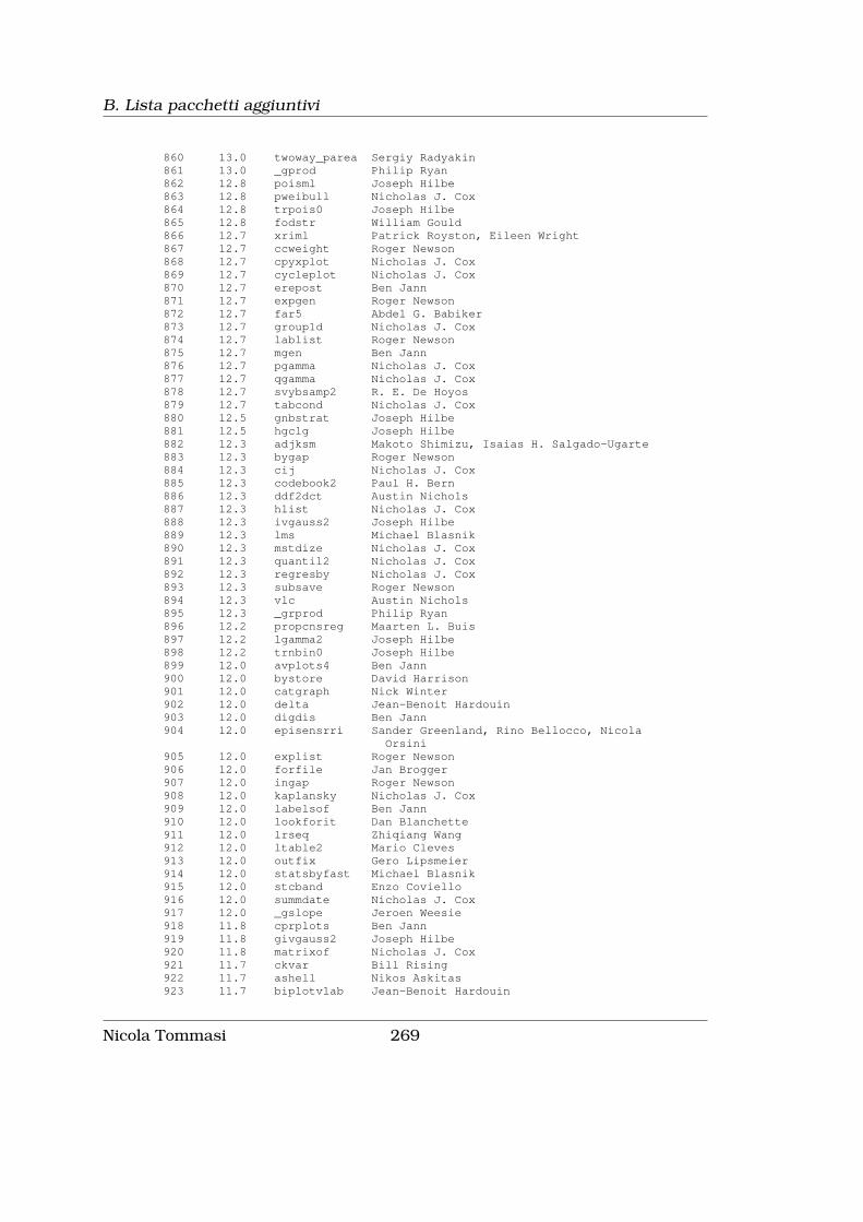
B. Lista pacchetti aggiuntivi
860 13.0 twoway_parea Sergiy Radyakin861 13.0 _gprod Philip Ryan862 12.8 poisml Joseph Hilbe863 12.8 pweibull Nicholas J. Cox864 12.8 trpois0 Joseph Hilbe865 12.8 fodstr William Gould866 12.7 xriml Patrick Royston, Eileen Wright867 12.7 ccweight Roger Newson868 12.7 cpyxplot Nicholas J. Cox869 12.7 cycleplot Nicholas J. Cox870 12.7 erepost Ben Jann871 12.7 expgen Roger Newson872 12.7 far5 Abdel G. Babiker873 12.7 group1d Nicholas J. Cox874 12.7 lablist Roger Newson875 12.7 mgen Ben Jann876 12.7 pgamma Nicholas J. Cox877 12.7 qgamma Nicholas J. Cox878 12.7 svybsamp2 R. E. De Hoyos879 12.7 tabcond Nicholas J. Cox880 12.5 gnbstrat Joseph Hilbe881 12.5 hgclg Joseph Hilbe882 12.3 adjksm Makoto Shimizu, Isaias H. Salgado-Ugarte883 12.3 bygap Roger Newson884 12.3 cij Nicholas J. Cox885 12.3 codebook2 Paul H. Bern886 12.3 ddf2dct Austin Nichols887 12.3 hlist Nicholas J. Cox888 12.3 ivgauss2 Joseph Hilbe889 12.3 lms Michael Blasnik890 12.3 mstdize Nicholas J. Cox891 12.3 quantil2 Nicholas J. Cox892 12.3 regresby Nicholas J. Cox893 12.3 subsave Roger Newson894 12.3 vlc Austin Nichols895 12.3 _grprod Philip Ryan896 12.2 propcnsreg Maarten L. Buis897 12.2 lgamma2 Joseph Hilbe898 12.2 trnbin0 Joseph Hilbe899 12.0 avplots4 Ben Jann900 12.0 bystore David Harrison901 12.0 catgraph Nick Winter902 12.0 delta Jean-Benoit Hardouin903 12.0 digdis Ben Jann904 12.0 episensrri Sander Greenland, Rino Bellocco, Nicola
Orsini905 12.0 explist Roger Newson906 12.0 forfile Jan Brogger907 12.0 ingap Roger Newson908 12.0 kaplansky Nicholas J. Cox909 12.0 labelsof Ben Jann910 12.0 lookforit Dan Blanchette911 12.0 lrseq Zhiqiang Wang912 12.0 ltable2 Mario Cleves913 12.0 outfix Gero Lipsmeier914 12.0 statsbyfast Michael Blasnik915 12.0 stcband Enzo Coviello916 12.0 summdate Nicholas J. Cox917 12.0 _gslope Jeroen Weesie918 11.8 cprplots Ben Jann919 11.8 givgauss2 Joseph Hilbe920 11.8 matrixof Nicholas J. Cox921 11.7 ckvar Bill Rising922 11.7 ashell Nikos Askitas923 11.7 biplotvlab Jean-Benoit Hardouin
Nicola Tommasi 269

B. Lista pacchetti aggiuntivi
924 11.7 clustsens Paul Millar925 11.7 cquantile Nicholas J. Cox926 11.7 difwithpar Laura Gibbons927 11.7 ds5 Nicholas J. Cox928 11.7 geneigen Christopher F Baum929 11.7 gumbelfit Stephen P. Jenkins, Nicholas J. Cox930 11.7 kapprevi Debora Rizzuto, Nicola Orsini931 11.7 lincom2 Jan Brogger932 11.7 mkbilogn Stephen P. Jenkins933 11.7 raschcvt Fred Wolfe934 11.7 rowsort Nicholas J. Cox935 11.7 soepren Ulrich Kohler936 11.6 contrast Patrick Royston937 11.5 fiskfit Maarten L. Buis, Stephen P. Jenkins938 11.5 trinary David Kantor939 11.4 mcqscore E. Paul Wileyto940 11.3 bmjcip Roger Newson941 11.3 cctable Peter Makary, Gilles Desve942 11.3 copydesc Nicholas J. Cox943 11.3 dashln Michael Blasnik944 11.3 dbmscopybatch Amadou Bassirou Diallo945 11.3 factmerg Roger Newson946 11.3 palette_all Adrian Mander947 11.3 ranvar Frauke Kreuter948 11.3 slist Jens M. Lauritsen, Svend Juul, John
Luke Gallup949 11.3 spec_stand Rosa Gini950 11.3 sqr Nicholas J. Cox951 11.3 stcumh Kim Lyngby Mikkelsen952 11.3 survtime Allen Buxton953 11.2 dagumfit Stephen P. Jenkins954 11.2 adotype Nicholas J. Cox955 11.2 cenpois Joseph Hilbe, Dean Judson956 11.2 qhapipf Adrian Mander957 11.2 qweibull Nicholas J. Cox958 11.2 williams Joseph Hilbe959 11.0 bkrosenblatt Nicholas J. Cox960 11.0 canon Bill Sribney961 11.0 cvxhull R. Allan Reese962 11.0 distan Jose Maria Sanchez Saez963 11.0 gphepssj Roger Newson964 11.0 labelmiss Stanislav Kolenikov965 11.0 lars Adrian Mander966 11.0 mfilegr Philip Ryan967 11.0 mnthplot Nicholas J. Cox968 11.0 muxplot Nicholas J. Cox969 11.0 nbinreg Joseph Hilbe970 11.0 svypxcat Joanne M. Garrett971 11.0 svypxcon Joanne M. Garrett972 10.9 jnsn Joseph Coveney973 10.9 lmoments Nicholas J. Cox974 10.8 cprplot2 Ben Jann975 10.8 adolist Stefan Wehrli, Ben Jann976 10.7 checkvar Phil Bardsley977 10.7 dashgph Nick Winter978 10.7 disjoint Nicholas J. Cox979 10.7 epiconf Zhiqiang Wang980 10.7 grexport Lars E. Kroll981 10.7 linkplot Nicholas J. Cox982 10.7 matpwcorr Adrian Mander983 10.7 qqplot2 Nicholas J. Cox984 10.7 shownear Nicholas J. Cox985 10.7 spaces Jan Brogger986 10.7 spellutil Edwin Leuven987 10.7 sunflower W. Dale Plummer Jr., William D. Dupont
270 Nicola Tommasi

B. Lista pacchetti aggiuntivi
988 10.7 swapval Nicholas J. Cox989 10.7 symmetry Mario Cleves990 10.5 marktouse Ben Jann991 10.3 casefat Jamie Griffin, Azra Ghani992 10.3 confall Zhiqiang Wang993 10.3 confnd Zhiqiang Wang994 10.3 coranal Philippe Van Kerm995 10.3 doubmass Nicholas J. Cox996 10.3 ds2 Nicholas J. Cox997 10.3 getfilename2 Jeff Arnold998 10.3 hdquantile Nicholas J. Cox999 10.3 himatrix Ulrich Kohler1000 10.3 insob Bas Straathof1001 10.3 muxyplot Nicholas J. Cox1002 10.3 ztg Joseph Hilbe1003 10.2 mkstrsn William Gould1004 10.2 mlboolean Bear F. Braumoeller1005 10.2 psbayes Nicholas J. Cox1006 10.2 qbeta Nicholas J. Cox1007 10.2 rdci Joseph Coveney1008 10.2 tcod Mamoun BenMamoun1009 10.0 blist Adrian Mander1010 10.0 blogit2 Nicholas J. Cox1011 10.0 bys Jeroen Weesie1012 10.0 for211 Patrick Royston1013 10.0 fractileplot Nicholas J. Cox1014 10.0 fview Ben Jann1015 10.0 glmcorr Nicholas J. Cox1016 10.0 gphodp Peter Parzer1017 10.0 irrepro Nicholas J. Cox1018 10.0 postrri Sander Greenland, Rino Bellocco, Nicola
Orsini1019 10.0 printgph Jan Brogger1020 10.0 sssplot Nicholas J. Cox1021 10.0 torats Nicholas J. Cox, Christopher F Baum1022 10.0 unitab Nicola Orsini, Matteo Bottai1023 10.0 varsearch Jeff Arnold1024 9.9 sdtest Bill Sribney1025 9.8 ncf Thomas Steichen1026 9.7 allcross Kenneth Higbee1027 9.7 ascii Adrian Mander1028 9.7 buckley James Cui1029 9.7 diplot Nicholas J. Cox1030 9.7 doubletofloat David Kantor1031 9.7 gprefscode Jan Brogger1032 9.7 pascal Amadou Bassirou Diallo1033 9.7 tolerance Peter Lachenbruch1034 9.5 hnbreg1 Joseph Hilbe1035 9.5 simuped James Cui1036 9.5 sortrows Jeff Arnold1037 9.4 wtd Henrik Stovring1038 9.3 convert_top_lines David Kantor1039 9.3 effcon Al Feiveson1040 9.3 hsmode Nicholas J. Cox1041 9.3 intterms Vince Wiggins1042 9.3 ndbci Fred Wolfe1043 9.3 nicedates Nicholas J. Cox1044 9.3 pnrcheck Nicola Orsini1045 9.3 showgph Jan Brogger, Nicholas J. Cox1046 9.3 shuffle8 Ben Jann1047 9.3 spikeplt Tony Brady, Nicholas J. Cox1048 9.0 gen_tail David Kantor1049 9.0 loopplot Nicholas J. Cox1050 9.0 skilmack Mark Chatfield1051 9.0 storecmd Nicholas J. Cox
Nicola Tommasi 271
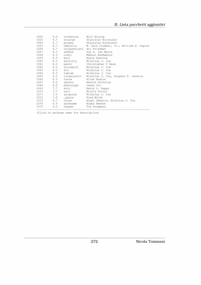
B. Lista pacchetti aggiuntivi
1052 9.0 vtokenize Bill Rising1053 8.7 enlarge Stanislav Kolenikov1054 8.7 primes Stanislav Kolenikov1055 8.7 umbrella W. Dale Plummer, Jr., William D. Dupont1056 8.7 uniquestrata Ari Friedman1057 8.3 addtex Guy D. van Melle1058 8.3 codci Mamoun BenMamoun1059 8.3 mail Nikos Askitas1060 8.3 majority Nicholas J. Cox1061 8.3 pwcov Christopher F Baum1062 8.3 sliceplot Nicholas J. Cox1063 8.3 sto Nicholas J. Cox1064 8.3 tablab Nicholas J. Cox1065 8.3 invgaussfit Nicholas J. Cox, Stephen P. Jenkins1066 8.2 tarow Allen Buxton1067 8.2 rpnfcn Henrik Stovring1068 8.0 phenotype James Cui1069 7.7 eitc Kerry L. Papps1070 7.7 esli Nicola Orsini1071 7.5 qlognorm Nicholas J. Cox1072 7.0 _grpos Fred Wolfe1073 6.7 nruns Nigel Smeeton, Nicholas J. Cox1074 6.5 qrowname Roger Newson1075 4.0 soepdo Tim Stegmann----------------------------------------------------------------------(Click on package name for description)
272 Nicola Tommasi
To Do
- limits (fatto!!) e labutils (questo fatto??)- numlabel _all, add- labelsof- fre - groups- preserve ... restore- Costruzione di successioni del tipo a, b, c oppure
aa, ab, ac...ba, bb, bc...per sistemi AIDS
- contract [FF... FFFATTO!] e xpose- outliers analysis [FF... FFFATTO!]- spmap + correzione centroidi e in Appendice l’help con le figure- ameans, centile e cumul- egen agegp=cut(e2), at(0,5,10,15,20,25,30,35,40,45,50,55,60,65,70,75,80,100)
[FATTO] label define agegp 0 0-4 5 5-9 10 10-14 15 15-19 20 20-25 2525-29 30 30-34 35 35-39 40 40-44 45 45-49 50 50-54 55 55-59 60 60-6465 65-69 70 70-74 75 75-79 80 80+ [FF... FFFATTO!]
- label values now takes a varlist [FF... FFFATTO!].- xmlsave [FATTO]- mrtab- labelbook- adopath- ds undocumented command ( ds, not(type string); recode ‘r(varlist)’ (.=.a);
marina -> farmaci)- listblck- utilizzo di ++ e – per i cicli delle local. Attenzione che ++local lascia poi la
local aumentata di 1- qui recode a14 (1=1 0 - 9) (3=2 10-19) (4 5=3 20 - 39), gen(a14rec);- nuova opzione firstonly per tab2
CASI APPLICATI
- Prezzi alla Lewbel
273
B. To Do
- strmatch per correzione stradario- Arrotondamento local- run----
How do I send Stata output to Technical Support?If you need to send output to Technical Support, use the following procedure:
. log using junk, replace. about. update. sysdir. adopath. pwd. describe. summarize. <command(s) causing problems>. log close
These commands will create the file junk.smcl, which you can then email tous.
projects/s_cuore/marina/farmaci/read.do
label define tipof 1 "Apparato gastrointestinale e matabolismo (A)"2 "Sangue e organi emopoietici (B)"3 "Sistema cardiovascolare (C)"4 "Sistema genito-urinario (G)"5 "Preparati ormonali sistemici, esclusi gli ormoni sessuali (H)"6 "Antimicrobici generali per uso sistemico eimmunomodulatori (J)"7 "Farmaci antineoplastici e immunomodulatori (L)"8 "Sistema muscolo-scheletrico (M)"9 "Sistema nervoso (N)"10 "Sistema respiratorio"11 "Organi di senso (S)";
recode a23t* (1/16 =1) (17/21=2) (22/34=3) (35/37=4) (38/42=5) (43/46=6) (47/50=7) (51/56=8) (57/63=9) (64/69=10) (70/71=11),prefix(cat_) label(tipof);
274 Nicola Tommasi

Parte IV
Indici
275


Indice analitico
*, 32==, 31?, 32&, 32_N, 81_n, 81|, 32>, 31<, 31,̃ 32˜=, 31>=, 31
abbrev, 73about, 8abs, 69adoupdate, 21aorder, 64append, 115
betaden, 71binomial, 71box, 111by, 33, 82bysort, 34, 82
ceil, 69chi2, 72codebook, 52collapse, 123colsof, 79compress, 40cond, 76contract, 128correlate, 108
dati missing, 32, 34
decode, 88delimit, 17delimitatori fine comando, 17describe, 51destring, 88diag, 78dictionary, 42, 44dir, 16directory di lavoro, 15drop, 64duplicates report, 61
egen, 83egenmore, 83egenodd, 83encode, 88erase, 16ereturn list, 148excel, 47exp, 70
F, 72Fden, 72findit, 21finestra Review, 3finestra Stata Command, 3finestra Stata Results, 3finestra Variables, 3floor, 69foreach, 141format, 66forvalues, 146fre, 95fsum, 94Funioni di probabilita’, 71Funzioni di densita’, 71
277

INDICE ANALITICO INDICE ANALITICO
Funzioni matematiche, 69Funzioni random, 73Funzioni stringa, 73
gammaden, 72generate, 69global, 139grubbs, 110gsort, 63
help, 21
if, 30in, 29infile, 42inlist, 76, 86inputst, 45inrange, 77insheet, 41inspect, 53int, 69inv, 79invnormal, 73
keep, 64
label data, 54label define, 55label dir, 56label drop, 56label list, 56label values, 55label variable, 54labelbook, 57labutil, 59labvalch, 56lenght, 73limits, 5ln, 70local, 139, 147log, 19log10, 70long form, 124lower, 74ltrim, 74
macros, 139max, 70, 84mdy, 77mean, 84median, 85merge, 116mif2dta, 151min, 71, 85mkdir, 16mmerge, 118mode, 86move, 64
normalden, 72notes, 60nullmat, 80numlabel, 59
operatori di relazione, 31operatori logici, 32order, 64outliers, 109outputst, 45outsheet, 46
preserve, 47pwcorr, 109pwd, 15
r(), 149recast, 66recode, 87rename, 62renvars, 62replace, 86reshape, 124restore, 47reverse, 74round, 69rowmax, 86rowmean, 86rowmin, 86rowmiss, 86rownomiss, 86rowsd, 86
278 Nicola Tommasi

INDICE ANALITICO INDICE ANALITICO
rowsof, 79rtrim, 74
sample, 65scalar, 141search, 21separatori, 28set dp, 68set memory, 37set seed, 65set varlabelpos, 5shp2dta, 151SO supportati, 3sort, 63spmap, 193ssc, 20strmatch, 74subinstr, 75subinword, 75substr, 75sum, 71, 86summarize, 93sysdir, 11
tab2, 102table, 104tabstat, 106tabulate, 94tipo variabili, 66tostring, 89trace, 81trim, 74
uniform, 73update, 19upper, 74use, 27, 39
versioni, 3
wide form, 124word, 75wordcount, 76
XML, 46
xmlsave, 46xmluse, 47
Nicola Tommasi 279


Elenco delle figure
1 II Incontro degli Utenti di Stata, Milano, 10-11 ottobre 2005 . . . iii
1.1 Le finestre di Stata . . . . . . . . . . . . . . . . . . . . . . . . . . . . 4
9.1 Box Plot . . . . . . . . . . . . . . . . . . . . . . . . . . . . . . . . . . 112
14.1Mappa pre correzione . . . . . . . . . . . . . . . . . . . . . . . . . . 15314.2Mappa post correzione . . . . . . . . . . . . . . . . . . . . . . . . . 15514.3Mappa con colori predefiniti . . . . . . . . . . . . . . . . . . . . . . 15614.4Mappa con colori assegnati . . . . . . . . . . . . . . . . . . . . . . . 158
A.1 Choropleth maps . . . . . . . . . . . . . . . . . . . . . . . . . . . . . 225A.2 Choropleth maps . . . . . . . . . . . . . . . . . . . . . . . . . . . . . 226A.3 Choropleth maps . . . . . . . . . . . . . . . . . . . . . . . . . . . . . 227A.4 Choropleth maps . . . . . . . . . . . . . . . . . . . . . . . . . . . . . 228A.5 Choropleth maps . . . . . . . . . . . . . . . . . . . . . . . . . . . . . 229A.6 Choropleth maps . . . . . . . . . . . . . . . . . . . . . . . . . . . . . 230A.7 Choropleth maps . . . . . . . . . . . . . . . . . . . . . . . . . . . . . 231A.8 Choropleth maps . . . . . . . . . . . . . . . . . . . . . . . . . . . . . 232A.9 Choropleth maps . . . . . . . . . . . . . . . . . . . . . . . . . . . . . 233A.10Choropleth maps . . . . . . . . . . . . . . . . . . . . . . . . . . . . . 234A.11Choropleth maps . . . . . . . . . . . . . . . . . . . . . . . . . . . . . 235A.12Choropleth maps . . . . . . . . . . . . . . . . . . . . . . . . . . . . . 236A.13Proportional symbol maps . . . . . . . . . . . . . . . . . . . . . . . 237A.14Proportional symbol maps . . . . . . . . . . . . . . . . . . . . . . . 238A.15Proportional symbol maps . . . . . . . . . . . . . . . . . . . . . . . 239A.16Proportional symbol maps . . . . . . . . . . . . . . . . . . . . . . . 240A.17Proportional symbol maps . . . . . . . . . . . . . . . . . . . . . . . 241A.18Other maps . . . . . . . . . . . . . . . . . . . . . . . . . . . . . . . . 242A.19Other maps . . . . . . . . . . . . . . . . . . . . . . . . . . . . . . . . 243A.20Other maps . . . . . . . . . . . . . . . . . . . . . . . . . . . . . . . . 244A.21Other maps . . . . . . . . . . . . . . . . . . . . . . . . . . . . . . . . 245A.22Other maps . . . . . . . . . . . . . . . . . . . . . . . . . . . . . . . . 246A.23Other maps . . . . . . . . . . . . . . . . . . . . . . . . . . . . . . . . 247
281

ELENCO DELLE FIGURE ELENCO DELLE FIGURE
A.24Other maps . . . . . . . . . . . . . . . . . . . . . . . . . . . . . . . . 248A.25Other maps . . . . . . . . . . . . . . . . . . . . . . . . . . . . . . . . 249A.26Other maps . . . . . . . . . . . . . . . . . . . . . . . . . . . . . . . . 250
282 Nicola Tommasi

Elenco delle tabelle
283


