1

Stat 401B Exam 2 Fall 2016

I have neither given nor received unauthorized assistance on this exam.

________________________________________________________ Name Signed Date

_________________________________________________________ Name Printed

ATTENTION! Incorrect numerical answers unaccompanied by supporting reasoning will receive NO partial credit. Correct numerical answers to difficult questions unaccompanied by supporting reasoning may not receive full credit. SHOW YOUR WORK/EXPLAIN YOURSELF! Completely absurd answers (that fail basic sanity checks but that you don't identify as clearly incorrect) may receive negative credit.

2

1. A shop uses spot welding to join two parts of an assembly. Two different machines are used to make the same welds. Measured strengths for welds from the machines are summarized below.

Machine #1 Machine #2 1 25n = 2 25n =

1 1461.7 psix = 2 1538.1 psix =

1 324.5 psis = 2 280.3 psis = number above 1800 psi 1= number above 1800 psi 7= number below 1100 psi 3= number below 1100 psi 0=

a) Strengths below 1100 psi or above 1800 psi are undesirable/nonconforming. Is there clear evidence of a difference between the two machines in terms of the fractions of nonconforming welds they produce? (Show the whole 5-step format.) b) Give 90% two-sided confidence limits for comparing the standard deviations of weld strengths produced by the two machines. c) On the basis of your limits from b) can you say with fair certainty which machine produces more consistent weld strengths? Why or why not?

3 pts

6 pts

8 pts

3

Below are normal plots for the weld strengths for the two machines made on the same set of axes.

d) What does the plot indicate about the two distributions of weld strengths? e) Give (small sample) two-sided 95% confidence limits for the difference in mean weld strengths for the two machines. f) If one judged the plot at the top of the page to fail to be approximately linear for one or both of the two machines, what basis might there nevertheless be for hoping that the nominal 95% confidence level used in e) is not ridiculously wrong as characterizing the reliability of the formula you used? g) Would the same reasoning you applied in f) extend to use of the tolerance limits 2x sτ± ? Explain.

3 pts

5 pts

6 pts

3 pts

4

2. At the end of this exam there is an R printout that concerns analysis of data from a study of the surface finish produced in a machining operation. A response variable, y , measuring a characteristic of surface finish related to ultimate part strength was studied as a function of machine settings. The first input variable, speed rate, was originally in rpm and has been coded by subtraction of 3500 and then division by 1000 to produce values of the variable 1x . The second input variable, feed rate, was originally in inches/revolution and has been coded by subtraction of .005 and then division by .004 to produce values of the variable 2x . To begin, consider only the data with 1 1x = − (the lowest speed rate). Notice that from one perspective this amounts to 3r = samples, each of size 2 ( 1 2 3 2n n n= = = ). a) Give two-sided 95% confidence limits for the standard deviation of y for any fixed feed rate (at this lowest speed rate) under the one-way normal model. b) Give values of an F statistic and degrees of freedom for testing the hypothesis that (at this lowest speed rate) feed rate has no effect on average y . Is this hypothesis plausible? F = ____________ d.f. = ______ , ______ Plausible? __________ c) Because the values of the variable 2x are equally spaced, the quantity ( ) ( )2 2 2 2(mean for 1) (mean for 0) (mean for 0) (mean for 1)y x y x y x y x= − = − = − = − is a measure of "curvature" or second derivative in mean response (at this lowest speed rate). Give and interpret 95% two-sided confidence limits for this quantity.

8 pts

6 pts

6 pts

5

Continue to consider only the data with 1 1x = − (the lowest speed rate), but now treat a regression analysis with the predictor variable 2x . d) What fraction of the raw variation in y (at this lowest speed rate) can be "accounted for" using a model linear in 2x ? e) Give 95% two-sided confidence limits for the standard deviation of y at any fixed value of 2x under the SLR model (at this lowest speed rate). How does this compare to your answer to a)? Why, in retrospect, is this similarity or difference understandable? f) Give 95% two-sided confidence limits for the increase in mean y associated with a .001 inch/revolution increase in feed rate (according to the SLR analysis at this lowest speed rate). (Hint: look again at the top of the previous page and the description of how 2x was coded. What would the answer here be if it was a "1 unit increase in 2x " that was under discussion?) g) Give 95% prediction limits (based on the SLR model at this lowest at rate) the next y observed at

2 1x = . (Plug in completely, but you need not simplify.)

6 pts

6 pts

6 pts

4 pts

6

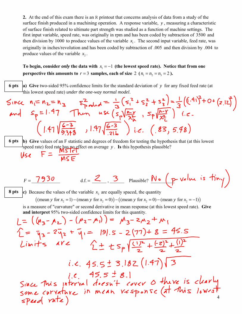
Finally consider all the data and both 1x and 2x . There are several regressions reported on the output for the entire data set. Use them in answering the following. h) Over the ranges represented by the data used here, which of the predictors ( 1 2 or x x ) is most important in modeling y ? Give quantitative rationale for your answer. Variable: __________ Rationale: i) Give 95% two-sided confidence limits for the increase in mean y associated with a unit increase in

1x when 2x is held fixed. j) Give and interpret 95% two sided confidence limits for the intercept in the MLR model including both 1 2 and x x for this particular data set. k) What is the value of the sample correlation between the response and the predicted response for MLR including both 1 2 and x x ? l) Give 95% two-sided prediction limits for the next y when 1 20 and 0x x= = . (You don't need a special prediction call to get ˆˆ or se yy here. Consider again part j).)

6 pts

4 pts

5 pts

6 pts

5 pts

7

R Code and Output > x1<-c(rep(-1,6),rep(0,6),rep(1,6)) > x2<-c(rep(c(-1,-1,0,0,1,1),3)) > treat<-c(1,1,2,2,3,3,4,4,5,5,6,6,7,7,8,8,9,9) > y<-c(7,9,77,77,193,190,7,9,75,85,191,191,9,18,79,80,192,190) > cbind(treat,x1,x2,y) treat x1 x2 y [1,] 1 -1 -1 7 [2,] 1 -1 -1 9 [3,] 2 -1 0 77 [4,] 2 -1 0 77 [5,] 3 -1 1 193 [6,] 3 -1 1 190 [7,] 4 0 -1 7 [8,] 4 0 -1 9 [9,] 5 0 0 75 [10,] 5 0 0 85 [11,] 6 0 1 191 [12,] 6 0 1 191 [13,] 7 1 -1 9 [14,] 7 1 -1 18 [15,] 8 1 0 79 [16,] 8 1 0 80 [17,] 9 1 1 192 [18,] 9 1 1 190 > aggregate(y,by=list(treat),mean) Group.1 x 1 1 8.0 2 2 77.0 3 3 191.5 4 4 8.0 5 5 80.0 6 6 191.0 7 7 13.5 8 8 79.5 9 9 191.0 > aggregate(y,by=list(treat),sd) Group.1 x 1 1 1.4142136 2 2 0.0000000 3 3 2.1213203 4 4 1.4142136 5 5 7.0710678 6 6 0.0000000 7 7 6.3639610 8 8 0.7071068 9 9 1.4142136 > summary(aov(y[1:6] ~ as.factor(x2[1:6]))) Df Sum Sq Mean Sq F value Pr(>F) as.factor(x2[1:6]) 2 34362 17181 7930 2.6e-06 *** Residuals 3 6 2 --- Signif. codes: 0 ‘***’ 0.001 ‘**’ 0.01 ‘*’ 0.05 ‘.’ 0.1 ‘ ’ 1

8

> summary(lm(y[1:6]~x2[1:6])) Call: lm(formula = y[1:6] ~ x2[1:6]) Residuals: 1 2 3 4 5 6 6.583 8.583 -15.167 -15.167 9.083 6.083 Coefficients: Estimate Std. Error t value Pr(>|t|) (Intercept) 92.167 5.387 17.11 6.85e-05 *** x2[1:6] 91.750 6.598 13.90 0.000155 *** --- Signif. codes: 0 ‘***’ 0.001 ‘**’ 0.01 ‘*’ 0.05 ‘.’ 0.1 ‘ ’ 1 Residual standard error: 13.2 on 4 degrees of freedom Multiple R-squared: 0.9797, Adjusted R-squared: 0.9747 F-statistic: 193.4 on 1 and 4 DF, p-value: 0.0001551 > summary(aov(y[1:6]~x2[1:6])) Df Sum Sq Mean Sq F value Pr(>F) x2[1:6] 1 33672 33672 193.4 0.000155 *** Residuals 4 697 174 --- Signif. codes: 0 ‘***’ 0.001 ‘**’ 0.01 ‘*’ 0.05 ‘.’ 0.1 ‘ ’ 1 > plot(x1,x2)

> plot(x1,y)

9

> plot(x2,y)

> summary(lm(y~x1)) Call: lm(formula = y ~ x1) Residuals: Min 1Q Median 3Q Max -86.28 -81.40 -15.03 96.97 100.97 Coefficients: Estimate Std. Error t value Pr(>|t|) (Intercept) 93.28 18.70 4.989 0.000134 *** x1 1.25 22.90 0.055 0.957138 --- Signif. codes: 0 ‘***’ 0.001 ‘**’ 0.01 ‘*’ 0.05 ‘.’ 0.1 ‘ ’ 1 Residual standard error: 79.32 on 16 degrees of freedom Multiple R-squared: 0.0001862, Adjusted R-squared: -0.0623 F-statistic: 0.00298 on 1 and 16 DF, p-value: 0.9571 > summary(lm(y~x2)) Call: lm(formula = y ~ x2) Residuals: Min 1Q Median 3Q Max -18.278 -12.028 6.056 6.889 15.389 Coefficients: Estimate Std. Error t value Pr(>|t|) (Intercept) 93.278 2.655 35.13 < 2e-16 *** x2 90.667 3.252 27.88 5.42e-15 *** --- Signif. codes: 0 ‘***’ 0.001 ‘**’ 0.01 ‘*’ 0.05 ‘.’ 0.1 ‘ ’ 1 Residual standard error: 11.26 on 16 degrees of freedom Multiple R-squared: 0.9798, Adjusted R-squared: 0.9786 F-statistic: 777.4 on 1 and 16 DF, p-value: 5.421e-15

10

> summary(lm(y~x1+x2)) Call: lm(formula = y ~ x1 + x2) Residuals: Min 1Q Median 3Q Max -18.278 -12.965 5.389 7.056 14.139 Coefficients: Estimate Std. Error t value Pr(>|t|) (Intercept) 93.278 2.729 34.174 1.21e-15 *** x1 1.250 3.343 0.374 0.714 x2 90.667 3.343 27.122 3.68e-14 *** --- Signif. codes: 0 ‘***’ 0.001 ‘**’ 0.01 ‘*’ 0.05 ‘.’ 0.1 ‘ ’ 1 Residual standard error: 11.58 on 15 degrees of freedom Multiple R-squared: 0.98, Adjusted R-squared: 0.9774 F-statistic: 367.9 on 2 and 15 DF, p-value: 1.797e-13 > summary(aov(y~x1+x2)) Df Sum Sq Mean Sq F value Pr(>F) x1 1 19 19 0.14 0.714 x2 1 98645 98645 735.60 3.68e-14 *** Residuals 15 2012 134 --- Signif. codes: 0 ‘***’ 0.001 ‘**’ 0.01 ‘*’ 0.05 ‘.’ 0.1 ‘ ’ 1