STAT-36700 Homework 7 - Solutionslarry/=stat700/HW07_sols.pdf · stat-36700 homework 7 - solutions 2 which implies that c0= c2 1,a since ( X m0 s/ p n)2 ˘c2 1 under H0.Then, by inverting

STAT-36700 Homework 7 - SolutionsFall 2018

October 28, 2018

This contains solutions for Homework 7. Please note that we haveincluded several additional comments and approaches to the problemsto give you better insight.

Problem 1. Let X1, . . . , Xn ∼ N (µ, σ2).

(a) Assume that σ2 is known. Invert the likelihood ratio test to construct anexact 1− α confidence interval for µ.

(b) Again, assume that σ2 is known. Invert the asymptotic likelihood ratiotest to construct an approximate 1− α confidence interval for µ.

(c) Now assume that σ2 is unknown. Invert the asymptotic likelihood ratiotest to construct an approximate 1− α confidence set for (µ, σ).

Solution 1. We derive each of the results below:

(a) For each µ0, we can construct an α level test of H0 : µ = µ0 versusH1 : µ 6= µ0 as follows:

λ(X1, . . . , Xn) =supµ∈Θ0

L(µ)

supµ∈Θ L(µ)

=L(µ0)

L(µ̂)where µ̂ = µ̂MLE = X

=exp(−∑n

i=1(Xi − µ0)2/(2σ2))

exp(−∑ni=1(Xi − X)2/(2σ2))

=exp(−∑n

i=1(Xi − X + X− µ0)2/(2σ2))

exp(−∑ni=1(Xi − X)2/(2σ2))

=exp(−∑n

i=1((Xi − X)2 + (X− µ0)2 + 2(Xi − X)(X− µ0))/(2σ2))

exp(−∑ni=1(Xi − X)2/(2σ2))

=exp(−∑n

i=1(Xi − X)2/(2σ2)) exp(−n(X− µ0)2/(2σ2))

exp(−∑ni=1(Xi − X)2/(2σ2))

sincen

∑i=1

(Xi − X) = 0

= exp(−n(X− µ0)2/(2σ2))

Hence, we reject H0 if

λ(X1, . . . , Xn) ≤ c⇐⇒ (X− µ0

σ/√

n)2 ≥ c′ for some c′

Then ( X−µ0σ/√

n )2 ≥ c′ becomes an α level test if

Pµ0((X− µ0

σ/√

n)2 ≥ c′) = α

stat-36700 homework 7 - solutions 2

which implies that c′ = χ21,α since ( X−µ0

σ/√

n )2 ∼ χ21 under H0. Then, by

inverting the test, we have that

Cn = {µ : (X− µ

σ/√

n)2 < χ2

1,α} = [X−

√χ2

1,α σ√

n, X +

√χ2

1,α σ√

n]

is a 1− α confidence interval for µ.

(b) The asymptotic likelihood ratio test claims that

−2 log λ(X1, . . . , Xn) χ21

since df = dim(Θ)− dim(Θ0) = 1− 0 = 1, which implies that

(X− µ0

σ/√

n)2 χ2

1

by calculations from part (a). Then

Pµ0((X− µ0

σ/√

n)2 ≥ χ2

1,α) = α

and the confidence interval for µ is (same as part (a))

Cn = [X−

√χ2

1,α σ√

n, X +

√χ2

1,α σ√

n]

by inverting the test.

(c)

λ(X1, . . . , Xn) =supµ,σ∈Θ0

L(µ, σ2)

supµ,σ∈Θ L(µ, σ2)

=L(µ0, σ̂2

0 )

L(µ̂, σ̂2)

where µ̂ = µ̂MLE = X, σ̂2 = σ̂2MLE = 1

n ∑ni=1(Xi − X)2, and

σ̂20 = 1

n ∑ni=1(Xi − µ0)

2. Then

λ(X1, . . . , Xn) = (σ̂

σ̂0)n exp(− 1

2σ̂20

n

∑i=1

(Xi − µ0)2 +

12σ̂2

n

∑i=1

(Xi − X)2)

= (σ̂

σ̂0)n exp(−n

2+

n2)

= (σ̂2

σ̂20)n/2

=∑n

i=1(Xi − X)2

∑ni=1(Xi − µ0)2


Hence, we reject at α level if

−2 log λ(X1, . . . , Xn) > χ21,α ⇐⇒ −2 log(

n

∑i=1

(Xi−X)2)+ 2 log(n

∑i=1

(Xi−µ0)2) > χ2

1,α

(again since df = dim(Θ) − dim(Θ0) = 1− 0 = 1) and thus 1− α

confidence interval for µ is

Cn = {µ : −2 log(n

∑i=1

(Xi − X)2) + 2 log(n

∑i=1

(Xi − µ)2) ≤ χ21,α}

by inverting the test.


Problem 2. Let X1, . . . , Xn ∼ Poisson(λ).

(a) By inverting the LRT, construct an approximate 1− α confidence set for λ

(b) Let λ = 10. Fix a value of n. Simulate n observations from thePoisson(λ) distribution. Construct your confidence set from part (a)and see if it includes the true value. Repeat this experiment 1000 timesto estimate the coverage probability. Plot the coverage as a function of n.Include your code as an appendix to the assignment.


(a) We claim that E(X) = µ.

Proof. For the Poisson distribution we have P(X = x) = e−λλx

x! . Sowe can derive the MLE as follows.

L(θ | x1, x2, . . . , xn) =n

∏i=1

e−λλxi

xi!

=(

e−nλλ∑ni=1 xi

) 1∏n

i=1 xi!

=⇒ l(θ | x1, x2, . . . , xn) = −nλ +n

∑i=1

xi log(λ)−n

∑i=1

log(xi)

=⇒ ∂l(θ | x1, x2, . . . , xn)

∂θ= −n +

∑ni=1 xi

λ

Setting this to 0 we have that

n =∑n

i=1 xi

λ

=⇒ λ = xn

Differentiating the log-likelihood, we have that

∂2l(λ | x1, x2, . . . , xn)

∂θ2 = −∑ni=1 xi

λ2

< 0

So ˆλMLE = Xn is the MLE.

Now we have that dim (Θ)− dim (Θ0) = 1− 0 = 1. So we don’treject the LRT (controlling for Type I error at α) if

−2 log(

L(λ0)

L(λ̂MLE)

)≤ χ2

1,α

−2 log

[exp (−n(λ0 − λ̂MLE))

(λ0

λ̂MLE

)nλ̂MLE]≤ χ2

1,α

⇐⇒ 2n[(λ0 − λ̂MLE)− λ̂MLE log

(λ0

λ̂MLE

)]≤ χ2

1,α

⇐⇒ λ0 − λ̂MLE log(λ0) ≤ λ̂MLE − λ̂MLE log(λ̂MLE) +χ2

1,α

2n


We can invert this expression for θ to give us the 1− α confidenceset for λ from the LRT as follows:

Cn =

{λ | λ− λ̂MLE log(λ) ≤ λ̂MLE − λ̂MLE log(λ̂MLE) +

χ21,α

2n

}

(b) We can use R to perform the approximation as follows:

# Clean uprm ( l i s t = l s ( ) )cat ( "\014" )

# L i b r a r i e s# i n s t a l l . p a c k a g e s (" t i d y v e r s e " )l i b r a r y ( t i d y v e r s e )

# S e t s e e d f o r r e p r o d u c i b i l i t yb a s e : : s e t . s e e d (7456445 )

# Setup p a r a m e t e r slambd _0 <− 10num_exp_ r e p l <− 1000a l p h <− 0 . 0 5num_ samps _ low <− 10num_ samps _ h igh <− 50010num_ samps _by <− 500

# H e lp e r f u n c t i o n s# Check t h a t our t r u e lambda _0 s a t i s f i e s our c o v e r a g e CI a t t h e a l p h a l e v e l# f o r t h e s p e c i f i e d number o f s i m u l a t e d s a m p l e s np o i s s _ l r t _cov <− funct ion ( lambd _ 0 , lambd _MLE, a lph , n ) {

b a s e : : r e turn ( lambd _0 − lambd _MLE* log ( lambd _ 0 ) <=lambd _MLE − lambd _MLE* log ( lambd _MLE) +s t a t s : : qchisq ( p = 1 − a lph , df = 1 ) / (2 *n ) )

}

# S i n g l e e x p e r i m e n ts i n g l e _ p o i s s _ e x p t <− funct ion ( n , lambd _ 0 , a l p h ) {

draw_ p o i s s <− s t a t s : : rpois ( n = n , lambda = lambd _ 0 )lambd _MLE <− b a s e : : mean ( draw_ p o i s s )c o n f _ s e t _cov <− p o i s s _ l r t _cov ( lambd _0 = lambd _ 0 , lambd _MLE = lambd _MLE,

a l p h = alph , n = n )b a s e : : r e turn ( c o n f _ s e t _cov )

}


# C r e a t e s e q u e n c e f o r n i . e . number o f p o i s s o n s a m p l e s t o draw f o r# e a c h r e p l i c a t i o nnum_ samps <− b a s e : : seq . i n t ( from = num_ samps _ low ,

t o = num_ samps _ high ,by = num_ samps _by )

# Run t h e e x p e r i m e n t s , f o r e a c h n , we r e p l i c a t e t h e e x p e r i m e n t# (num_ exp _ r e p l ) 1000 t i m e sout _exp <− p u r r r : : map ( . x = num_ samps ,

~ r e p l i c a t e ( n = num_exp_ r e p l ,expr = s i n g l e _ p o i s s _ e x p t ( n = . x ,

lambd _0 = lambd _ 0 ,a l p h = a l p h ) ) )

# For e a c h n , we measure c o v e r a g e p r o b a b i l i t y as a mean o f a l l# t i m e s c o v e r a g e was s a t i s f i e d in t h e r e p l i c a t i o n sout _exp_ covg <− p u r r r : : map_ d b l ( . x = out _exp , mean )

# We p l o t t h e c o v e r a g e p r o b a b i l i t y as a f u n c t i o n o f ncovg _ df <− t i b b l e : : t i b b l e ( n = num_ samps , covg _ prob = out _exp_ covg )covg _ plot <− covg _ df %>%

g g p l o t 2 : : g g p l o t ( data = . , a e s ( x = n , y = out _exp_ covg ) ) +g g p l o t 2 : : geom_ p o i n t ( ) +g g p l o t 2 : : geom_ l i n e ( ) +# Add t h e 1 − a l p h a l i n eg g p l o t 2 : : geom_ h l i n e ( y i n t e r c e p t =1−a lph , l i n e t y p e =" das he d " ,

c o l o r = " b l u e " , s i z e =1) +g g p l o t 2 : : y l im ( 0 . 6 , 1 ) +g g p l o t 2 : : l a b s ( t i t l e = " Coverage p r o b a b i l i t y o f lambda (= 10 ) vs n (1000 r e p l i c a t i o n s ) " ,

x = "Number o f s a m p l e s " ,y = " Coverage p r o b a b i l i t y " )

covg _ plot

We observe that as n increases the coverage probability becomes morestable around 1− α = 0.95 for alpha = 0.05


Plot:


Problem 3. Suppose we are given independent p-values P1, . . . , PN .

(a) Find the distribution of mini Pi when all the null hypothesis are true.

(b) Suppose we reject all null hypotheses such that Pi < t. Find the proba-bility of at least one false rejection when all the null hypothesis are true.Find t that makes this probability exactly α. How does this compare to theBonferroni rule?


(a) We claim that Fmini∈[N] Pi (γ) = 1− [1− γ]N .We note that for Homework 6, problem 3(a) that when the null hypothesisis true that the p-value is distributed as a Unif[0, 1] distribution. Nowusing this fact we have that under the global null all Pi ∼ Unif[0, 1](independent and identically distributed). Now let P(1) := mini∈[N] Pi

Proof.

FP(1)(γ) = P(

P(1) ≤ γ)

= 1−P(

P(1) > γ)

(Using complementary events)

= 1−P(∩i∈[N]{Pi > γ}

)(Since min implies all events greater than γ)

= 1− ∏i∈[n]

P(Pi > γ) (Using independence of Pi’s)

= 1− ∏i∈[N]

[1−P(Pi ≤ γ)] (Using complementary events)

= 1− ∏i∈[N]

[1− FPi (γ)

]= 1−

[1− FP1(γ)

]N(Since Pi’s are identically distributed)

= 1− (1− γ)N (Since Pi ∼ Unif[0, 1]∀i ∈ [N])

(b) We claim that t = 1− (1− α)1N .

Suppose we reject all null hypotheses such that Pi < t. Let I = {i |H0,i is true} Then given the independence of the tests we proceed asfollows:


Proof.

P(making atleast one false rejection) = P(Pi < t for some i ∈ I)

= P(∪i∈I{Pi < t})= 1−P(∩i∈I{Pi ≥ t}) (Using complementary events)

= 1−P

(mini∈[I]

Pi ≥ t)

(Re-expressing using setup from part (a))

= P

(mini∈[I]

Pi < t)

(Using complementary events)

= 1− (1− t)|I| (Using the CDF from part (a))

≤ 1− (1− t)N (given |I| ≤ N and t ∈ (0, 1))

Setting 1− (1− t)N = α we have that t = 1− (1− α)1N .

Comment

We note in general that by Taylor expansion that 1− (1− α)1N > α

nand as such assuming the tests are independent we note that Bon-ferroni correction is more conservative than the Sidak correctionproposed here. If the tests are not independent then we can’t usethis correction with guarantee and thus not directly comparable tothe Bonferroni correction.


Problem 4. Suppose we observe iid p-values P1, . . . , PN . Suppose that thedistribution for Pi is πU + (1 − π)G where 0 ≤ π ≤ 1, U denotes aUniform (0,1) distribution and G is some other distribution on (0, 1). Inother words, there is a probability π that H0 is true for each p-value.

(a) Suppose π is known. Suppose we use the rejection threshold defined bythe largest i such that P(i) < iα/(Nπ). Show that this controls thefalse discovery rate at level α. (Hint: use the proof in Lecture Notes 18.)Explain why this rule has higher power than the Benjamini-Hochbergthreshold.

(b) In practice π is not known. But we can estimate it as follows. Whenthe null is false, we expect the p-value to be near 0. To capture this idea,suppose that G is a distribution that puts all of its probability less than1/2. In other words, P(Pi < 1/2) = 1. Let π̂ = (1/N)∑i I(Pi > 1/2).Show that 2π̂ is a consistent estimator of π.

Solution 4.(a) Following the same logic as the proof in Lecture 18, let F bethe distribution of Pi, we have

E[FDP] ≈1N ∑N

i=1 WiE[I(Pi ≤ t)]1N ∑N

i=1 E[I(Pi ≤ t)]

=t|I|/N

F(t)

≈ tπF̂(t)

Let t = P(i) <iα

Nπ , then F̂(t) = i/N, and

E[FDP] ≤ iαNπ

π

i/N= α

Higher power than the Benjamini-Hochberg threshold because iαNπ > iα

Nand thus

max{j : P(j) <iα

Nπ} > max{j : P(j) <

iαN}.

This test has a bigger rejection region.

(b) First, notice that

E[I(Pi > 1/2)] = P(Pi > 1/2)

= 1−P(Pi ≤ 1/2)

= 1− [πU(1/2) + (1− π)G(1/2)]

= 1− π/2− 1 + π since G(1/2) = 1

= π/2


Then for all ε > 0,

P(|2π̂ − π| > ε) = P(| 1N

N

∑i=1

I(Pi > 1/2)− π

2| > ε

2)

≤Var( 1

N ∑Ni=1 I(Pi > 1/2))

ε2/4

=1N (E(I(Pi > 1/2)2)−E(I(Pi > 1/2))2)

ε2/4

=1N

π2 −

π2

4ε2/4

→ 0


Problem 5. In this question, we explore the frequentist properties of theBayesian posterior. Let X ∼ N(µ, 1). Let µ ∼ N(0, 1) be the prior for µ.

(a) Find the posterior p(µ|X).

(b) Find a(X) and b(X) such that∫ b(X)

a(X)p(µ|X)dµ = 0.95. In other words,

C = [a(X), b(X)] is the 95 percent Bayesian posterior interval.

(c) Now compute the frequentist coverage of C as a function of µ. In otherwords, fix the true value of the parameter µ. Now, treating µ as fixed andX ∼ N(µ, 1) as random, compute

Pµ(a(X) < µ < b(X)).

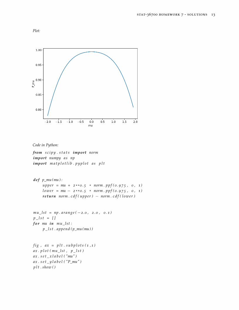
Plot this probability as a function of µ. Is the coverage probability equalto 0.95?

Solution 5. We note the solutions for each part as follows:

(a) See Lec Notes 17, example 2, the posterior distribution of µ is

µ|X ∼ N (X2

,12)

(b) Let µ|X ∼ N (X2 , 1

2 ), we want

P[a(X) ≤ µ ≤ b(X)] = 0.95

⇒ P[a(X)− X/2√

1/2≤ µ− X/2√

1/2≤ b(X)− X/2√

1/2] = 0.95

Thus

a(X) =X2−√

12

z0.025

b(X) =X2+

√12

z0.025

(c)

Pµ = P[X2−√

12

z0.025 < µ <X2+

√12

z0.025]

= P[µ−√

2 z0.025 < X− µ < µ +√

2 z0.025]

= Φ(µ +√

2 z0.025)−Φ(µ−√

2 z0.025)

The coverage probability is not 0.95. See the figure below.


Plot:

Code in Python:

from s c i p y . s t a t s import normimport numpy as npimport m a t p l o t l i b . p y p l o t a s p l t

def p_mu (mu ) :upper = mu + 2 * * 0 . 5 * norm . p p f ( 0 . 9 7 5 , 0 , 1 )l o w e r = mu − 2 * * 0 . 5 * norm . p p f ( 0 . 9 7 5 , 0 , 1 )r e turn norm . c d f ( upper ) − norm . c d f ( l o w e r )

mu_lst = np . a ran ge (−2 .0 , 2 . 0 , 0 . 1 )p _ l s t = [ ]f o r mu in mu_lst :

p _ l s t . append ( p_mu (mu ) )

f i g , ax = p l t . s u b p l o t s ( 1 , 1 )ax . p l o t ( mu_lst , p _ l s t )ax . s e t _ x l a b e l ( "mu" )ax . s e t _ y l a b e l ( "P_mu" )p l t . show ( )

Documents

STAT-36700 Homework 7 - Solutionslarry/=stat700/HW07_sols.pdf · stat-36700 homework 7 - solutions 2 which implies that c0= c2 1,a since ( X m0 s/ p n)2 ˘c2 1 under H0.Then, by inverting