Embed Size (px)
Citation preview

3 Creating a Model
3-2
Starting SimulinkTo start Simulink, you must first start MATLAB. Consult your MATLABdocumentation for more information. You can then start Simulink in two ways:
• Click on the Simulink icon on the MATLAB toolbar.
• Enter the simulink command at the MATLAB prompt.
On Microsoft Windows platforms, starting Simulink displays the SimulinkLibrary Browser.
The Library Browser displays a tree-structured view of the Simulink blocklibraries installed on your system. You can build models by copying blocks fromthe Library Browser into a model window (this procedure is described later inthis chapter).
On UNIX platforms, starting Simulink displays the Simulink block librarywindow.
The Simulink library window displays icons representing the block librariesthat come with Simulink. You can create models by copying blocks from thelibrary into a model window.

3-3
Note On Windows, you can display the Simulink library window byright-clicking the Simulink node in the Library Browser window.
Creating a New ModelTo create a new model, click the New button on the Library Browser’s toolbar(Windows only) or choose New from the library window’s File menu and selectModel. You can move the window as you do other windows. Chapter 2 describeshow to build a simple model. “Modeling Equations” on page 3–58 describes howto build systems that model equations.
Editing an Existing ModelTo edit an existing model diagram, either:
• Choose the Open button on the Library Browser’s toolbar (Windows only) orthe Open command from the Simulink library window’s File menu and thenchoose or enter the model filename for the model you want to edit.
• Enter the name of the model (without the .mdl extension) in the MATLABcommand window. The model must be in the current directory or on the path.
Entering Simulink CommandsYou run Simulink and work with your model by entering commands. You canenter commands by:
• Selecting items from the Simulink menu bar
• Selecting items from a context-sensitive Simulink menu (Windows only)
• Clicking buttons on the Simulink toolbar (Windows only)
• Entering commands in the MATLAB command window
Using the Simulink Menu Bar to Enter CommandsThe Simulink menu bar appears near the top of each model window. The menucommands apply to the contents of that window.
3 Creating a Model
3-4
Using Context-Sensitive Menus to Enter CommandsThe Windows version of Simulink displays a context-sensitive menu when youclick the right mouse button over a model or block library window. The contentsof the menu depend on whether a block is selected. If a block is selected, themenu displays commands that apply only to the selected block. If no block isselected, the menu displays commands that apply to a model or library as awhole.
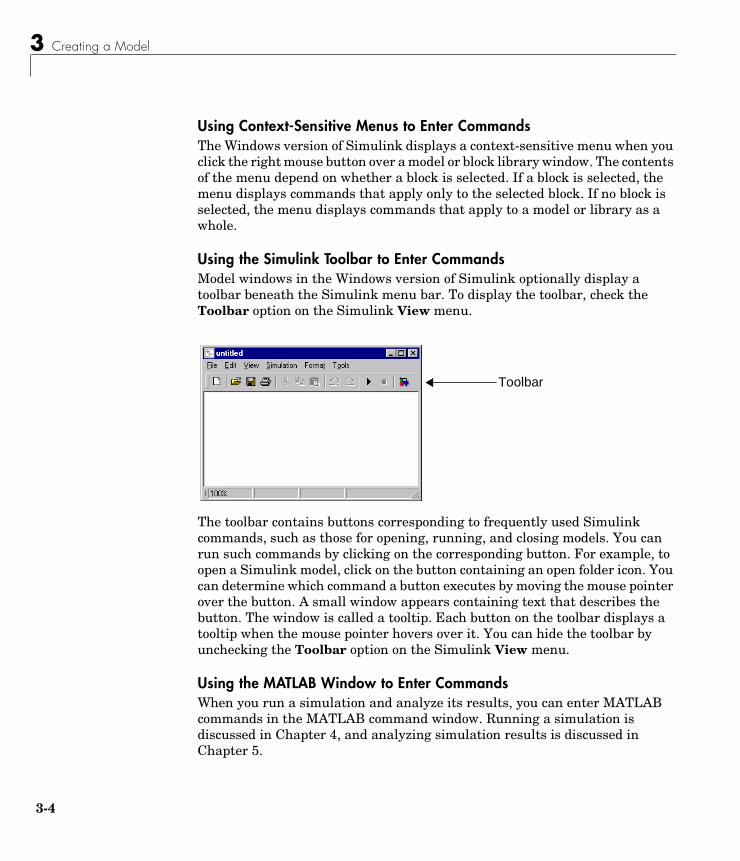
Using the Simulink Toolbar to Enter CommandsModel windows in the Windows version of Simulink optionally display atoolbar beneath the Simulink menu bar. To display the toolbar, check theToolbar option on the Simulink View menu.
The toolbar contains buttons corresponding to frequently used Simulinkcommands, such as those for opening, running, and closing models. You canrun such commands by clicking on the corresponding button. For example, toopen a Simulink model, click on the button containing an open folder icon. Youcan determine which command a button executes by moving the mouse pointerover the button. A small window appears containing text that describes thebutton. The window is called a tooltip. Each button on the toolbar displays atooltip when the mouse pointer hovers over it. You can hide the toolbar byunchecking the Toolbar option on the Simulink View menu.
Using the MATLAB Window to Enter CommandsWhen you run a simulation and analyze its results, you can enter MATLABcommands in the MATLAB command window. Running a simulation isdiscussed in Chapter 4, and analyzing simulation results is discussed inChapter 5.
Toolbar

3-5
Undoing a CommandYou can cancel the effects of up to 101 consecutive operations by choosing Undofrom the Edit menu. You can undo these operations:
• Adding or deleting a block
• Adding or deleting a line
• Adding or deleting a model annotation
• Editing a block name
You can reverse the effects of an Undo command by choosing Redo from theEdit menu.
Simulink WindowsSimulink uses separate windows to display a block library browser, a blocklibrary, a model, and graphical (scope) simulation output. These windows arenot MATLAB figure windows and cannot be manipulated using HandleGraphics® commands.
Simulink windows are sized to accommodate the most common screenresolutions available. If you have a monitor with exceptionally high or lowresolution, you may find the window sizes too small or too large. If this is thecase, resize the window and save the model to preserve the new windowdimensions.
Status BarThe Windows version of Simulink displays a status bar at the bottom of eachmodel and library window.
Status Bar

3 Creating a Model
3-6
When a simulation is running, the status bar displays the status of thesimulation, including the current simulation time and the name of the currentsolver. You can display or hide the status bar by checking or unchecking theStatus Bar item on the Simulink View menu.
Zooming Block DiagramsSimulink allows you to enlarge or shrink the view of the block diagram in thecurrent Simulink window. To zoom a view:
• Select Zoom In from the View menu (or type r) to enlarge the view.
• Select Zoom Out from the View menu (or type v) to shrink the view.
• Select Fit System to View from the View menu (or press the space bar) tofit the diagram to the view.
• Select Normal from the View menu to view the diagram at actual size.
By default, Simulink fits a block diagram to view when you open the diagrameither in the model browser’s content pane or in a separate window. If youchange a diagram’s zoom setting, Simulink saves the setting when you closethe diagram and restores the setting the next time you open the diagram. If youwant to restore the default behavior, choose Fit System to View from the Viewmenu the next time you open the diagram.

Selecting Objects
3-7
Selecting ObjectsMany model building actions, such as copying a block or deleting a line, requirethat you first select one or more blocks and lines (objects).
Selecting One ObjectTo select an object, click on it. Small black square “handles” appear at thecorners of a selected block and near the end points of a selected line. Forexample, the figure below shows a selected Sine Wave block and a selected line:
When you select an object by clicking on it, any other selected objects becomedeselected.
Selecting More than One ObjectYou can select more than one object either by selecting objects one at a time, byselecting objects located near each other using a bounding box, or by selectingthe entire model.
Selecting Multiple Objects One at a TimeTo select more than one object by selecting each object individually, hold downthe Shift key and click on each object to be selected. To deselect a selectedobject, click on the object again while holding down the Shift key.
Selecting Multiple Objects Using a Bounding BoxAn easy way to select more than one object in the same area of the window isto draw a bounding box around the objects.

3 Creating a Model
3-8
1 Define the starting corner of a bounding box by positioning the pointer atone corner of the box, then pressing and holding down the mouse button.Notice the shape of the cursor.
2 Drag the pointer to the opposite corner of the box. A dotted rectangleencloses the selected blocks and lines.
3 Release the mouse button. All blocks and lines at least partially enclosed bythe bounding box are selected.
Selecting the Entire ModelTo select all objects in the active window, choose Select All from the Editmenu. You cannot create a subsystem by selecting blocks and lines in this way;for more information, see “Creating Subsystems” on page 3–51.
Blocks
3-9
BlocksBlocks are the elements from which Simulink models are built. You can modelvirtually any dynamic system by creating and interconnecting blocks inappropriate ways. This section discusses how to use blocks to build models ofdynamic systems.
Block Data TipsOn Microsoft Windows, Simulink displays information about a block in apop-up window when you allow the pointer to hover over the block in thediagram view. To disable this feature or control what information a data tipincludes, select Block Data Tips from the Simulink View menu.
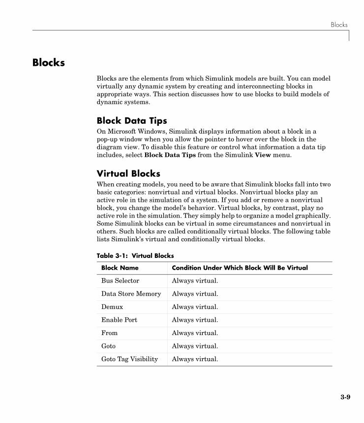
Virtual BlocksWhen creating models, you need to be aware that Simulink blocks fall into twobasic categories: nonvirtual and virtual blocks. Nonvirtual blocks play anactive role in the simulation of a system. If you add or remove a nonvirtualblock, you change the model’s behavior. Virtual blocks, by contrast, play noactive role in the simulation. They simply help to organize a model graphically.Some Simulink blocks can be virtual in some circumstances and nonvirtual inothers. Such blocks are called conditionally virtual blocks. The following tablelists Simulink’s virtual and conditionally virtual blocks.
Table 3-1: Virtual Blocks
Block Name Condition Under Which Block Will Be Virtual
Bus Selector Always virtual.
Data Store Memory Always virtual.
Demux Always virtual.
Enable Port Always virtual.
From Always virtual.
Goto Always virtual.
Goto Tag Visibility Always virtual.

3 Creating a Model
3-10
Copying and Moving Blocks from One Window to AnotherAs you build your model, you often copy blocks from Simulink block libraries orother libraries or models into your model window. To do this, follow these steps:
1 Open the appropriate block library or model window.
2 Drag the block you want to copy into the target model window. To drag ablock, position the cursor over the block icon, then press and hold down themouse button. Move the cursor into the target window, then release themouse button.
You can also drag blocks from the Simulink Library Browser into a modelwindow. See “Browsing Block Libraries” on page 3-25 for more information.
Ground Always virtual.
Inport Always virtual unless the block resides in aconditionally executed subsystem and has a directconnection to an outport block.
Mux Always virtual.
Outport Virtual if the block resides within any subsystemblock (conditional or not), and does not reside in theroot (top-level) Simulink window.
Selector Always virtual.
Subsystem Virtual if the block is not conditionally executed.
Terminator Always virtual.
Test Point Always virtual.
Trigger Port Virtual if the outport port is not present.
Table 3-1: Virtual Blocks (Continued)
Block Name Condition Under Which Block Will Be Virtual

Blocks
3-11
Note Simulink hides the names of Sum, Mux, Demux, and Bus Selectorblocks when you copy them from the Simulink block library to a model.This isdone to avoid unnecessarily cluttering the model diagram. (The shapes ofthese blocks clearly indicates their respective functions.)
You can also copy blocks by using the Copy and Paste commands from the Editmenu:
1 Select the block you want to copy.
2 Choose Copy from the Edit menu.
3 Make the target model window the active window.
4 Choose Paste from the Edit menu.
Simulink assigns a name to each copied block. If it is the first block of its typein the model, its name is the same as its name in the source window. Forexample, if you copy the Gain block from the Math library into your modelwindow, the name of the new block is Gain. If your model already contains ablock named Gain, Simulink adds a sequence number to the block name (forexample, Gain1, Gain2). You can rename blocks; see “Manipulating BlockNames” on page 3–16.
When you copy a block, the new block inherits all the original block’s parametervalues.
Simulink uses an invisible five-pixel grid to simplify the alignment of blocks.All blocks within a model snap to a line on the grid. You can move a blockslightly up, down, left, or right by selecting the block and pressing the arrowkeys.
You can display the grid in the model window by typing the following commandin the MATLAB window:
set_param('<model name>','showgrid','on')
To change the grid spacing, type:
set_param('<model name>','gridspacing',<number of pixels>)

3 Creating a Model
3-12
For example, to change the grid spacing to 20 pixels, type:
set_param('<model name>','gridspacing',20)
For either of the above commands, you can also select the model, and then typegcs instead of <model name>.
You can copy or move blocks to compatible applications (such as wordprocessing programs) using the Copy, Cut, and Paste commands. Thesecommands copy only the graphic representation of the blocks, not theirparameters.
Moving blocks from one window to another is similar to copying blocks, exceptthat you hold down the Shift key while you select the blocks.
You can use the Undo command from the Edit menu to remove an added block.
Moving Blocks in a ModelTo move a single block from one place to another in a model window, drag theblock to a new location. Simulink automatically repositions lines connected tothe moved block.
To move more than one block, including connecting lines:
1 Select the blocks and lines. If you need information about how to select morethan one block, see “Selecting More than One Object” on page 3–7.
2 Drag the objects to their new location and release the mouse button.
Duplicating Blocks in a ModelYou can duplicate blocks in a model as follows. While holding down the Ctrlkey, select the block with the left mouse button, then drag it to a new location.You can also do this by dragging the block using the right mouse button.Duplicated blocks have the same parameter values as the original blocks.Sequence numbers are added to the new block names.
Specifying Block ParametersThe Simulink user interface lets you assign values to block parameters. Someblock parameters are common to all blocks. Use the Block Properties dialogbox to set these parameters. To display the dialog box, select the block whose

Blocks
3-13
properties you want to set. Then select Block Properties... from Simulink’sEdit menu. See “Block Properties Dialog Box” on page 3-13 for moreinformation.
Other block parameters are specific to particular blocks. Use a block’sblock-specific parameter dialog to set these parameters. Double-click on theblock to open its dialog box. You can accept the displayed values or changethem. You can also use the set_param command to change block parameters.See set_param on page 10-24 for details.
Some block dialogs allow you to specify a data type for some or all of theirparameters.The reference material that describes each block (in Chapter 8)shows the dialog box and describes the block parameters.
Block Properties Dialog BoxThe Block Properties dialog box lets you set some common block parameters.
The dialog box contains the following fields:
DescriptionBrief description of the block’s purpose.
3 Creating a Model
3-14
PriorityExecution priority of this block relative to other blocks in the model. See“Assigning Block Priorities” on page 3-19 for more information.
TagA general text field that is saved with the block.
Open functionMATLAB (m-) function to be called when a user opens this block.
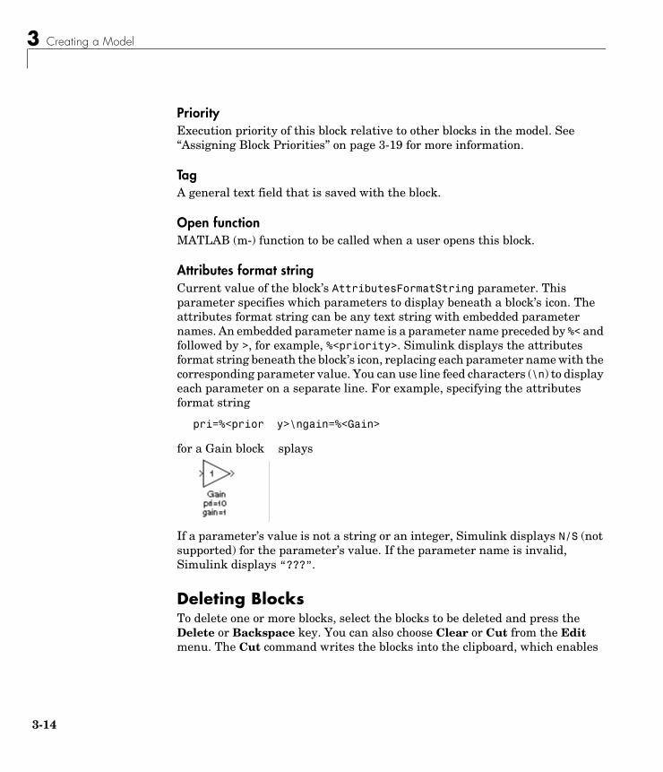
Attributes format stringCurrent value of the block’s AttributesFormatString parameter. Thisparameter specifies which parameters to display beneath a block’s icon. Theattributes format string can be any text string with embedded parameternames. An embedded parameter name is a parameter name preceded by %< andfollowed by >, for example, %<priority>. Simulink displays the attributesformat string beneath the block’s icon, replacing each parameter name with thecorresponding parameter value. You can use line feed characters (\n) to displayeach parameter on a separate line. For example, specifying the attributesformat string
pri=%<priority>\ngain=%<Gain>
for a Gain block displays
If a parameter’s value is not a string or an integer, Simulink displays N/S (notsupported) for the parameter’s value. If the parameter name is invalid,Simulink displays “???”.
Deleting BlocksTo delete one or more blocks, select the blocks to be deleted and press theDelete or Backspace key. You can also choose Clear or Cut from the Editmenu. The Cut command writes the blocks into the clipboard, which enables
Blocks
3-15
you to paste them into a model. Using the Delete or Backspace key or theClear command does not enable you to paste the block later.
You can use the Undo command from the Edit menu to replace a deleted block.
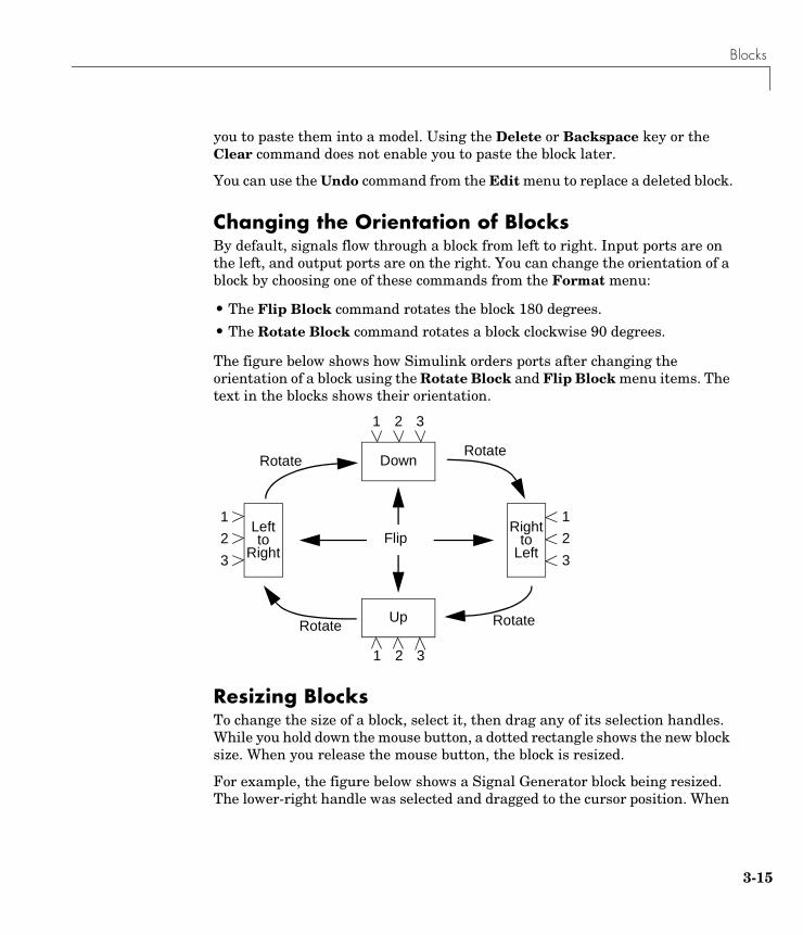
Changing the Orientation of BlocksBy default, signals flow through a block from left to right. Input ports are onthe left, and output ports are on the right. You can change the orientation of ablock by choosing one of these commands from the Format menu:
• The Flip Block command rotates the block 180 degrees.
• The Rotate Block command rotates a block clockwise 90 degrees.
The figure below shows how Simulink orders ports after changing theorientation of a block using the Rotate Block and Flip Block menu items. Thetext in the blocks shows their orientation.
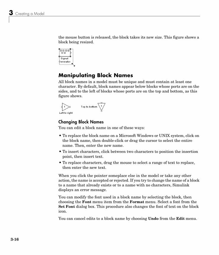
Resizing BlocksTo change the size of a block, select it, then drag any of its selection handles.While you hold down the mouse button, a dotted rectangle shows the new blocksize. When you release the mouse button, the block is resized.
For example, the figure below shows a Signal Generator block being resized.The lower-right handle was selected and dragged to the cursor position. When
1 2 3
Up
1
2
3
1 2 3
1
2
3
Rotate
RotateRotate
Rotate
Leftto
Right
Rightto
Left
Down
Flip
3 Creating a Model
3-16
the mouse button is released, the block takes its new size. This figure shows ablock being resized.
Manipulating Block NamesAll block names in a model must be unique and must contain at least onecharacter. By default, block names appear below blocks whose ports are on thesides, and to the left of blocks whose ports are on the top and bottom, as thisfigure shows.
Changing Block NamesYou can edit a block name in one of these ways:
• To replace the block name on a Microsoft Windows or UNIX system, click onthe block name, then double-click or drag the cursor to select the entirename. Then, enter the new name.
• To insert characters, click between two characters to position the insertionpoint, then insert text.
• To replace characters, drag the mouse to select a range of text to replace,then enter the new text.
When you click the pointer someplace else in the model or take any otheraction, the name is accepted or rejected. If you try to change the name of a blockto a name that already exists or to a name with no characters, Simulinkdisplays an error message.
You can modify the font used in a block name by selecting the block, thenchoosing the Font menu item from the Format menu. Select a font from theSet Font dialog box. This procedure also changes the font of text on the blockicon.
You can cancel edits to a block name by choosing Undo from the Edit menu.

Blocks
3-17
Note If you change the name of a library block, all links to that block willbecome unresolved.
Changing the Location of a Block NameYou can change the location of the name of a selected block in two ways:
• By dragging the block name to the opposite side of the block
• By choosing the Flip Name command from the Format menu. Thiscommand changes the location of the block name to the opposite side of theblock.
For more information about block orientation, see “Changing the Orientationof Blocks” on page 3–15.
Changing Whether a Block Name AppearsTo change whether the name of a selected block is displayed, choose a menuitem from the Format menu:
• The Hide Name menu item hides a visible block name. When you select HideName, it changes to Show Name when that block is selected.
• The Show Name menu item shows a hidden block name.
Displaying Parameters Beneath a Block’s IconYou can cause Simulink to display one or more of a block’s parameters beneaththe block’s icon in a block diagram. You specify the parameters to be displayedin the following ways:
• By entering an attributes format string in the Attributes format string fieldof the block’s Block Properties dialog box (see “Block Properties Dialog Box”on page 3-13)
• By setting the value of the block’s AttributesFormatString property to theformat string, using set_param (see set_param on page 10-24)
3 Creating a Model
3-18
Disconnecting BlocksTo disconnect a block from its connecting lines, hold down the Shift key, thendrag the block to a new location.
Vector Input and OutputAlmost all Simulink blocks accept scalar or vector inputs, generate scalar orvector outputs, and allow you to provide scalar or vector parameters. Theseblocks are referred to in this manual as being vectorized.
You can determine which lines in a model carry vector signals by choosingWide Vector Lines from the Format menu. When this option is selected, linesthat carry vectors are drawn thicker than lines that carry scalars. The figuresin the next section show scalar and vector lines.
If you change your model after choosing Wide Vector Lines, you mustexplicitly update the display by choosing Update Diagram from the Editmenu. Starting the simulation also updates the block diagram display.
Block descriptions in Chapter 8 discuss the characteristics of block inputs,outputs, and parameters.
Scalar Expansion of Inputs and ParametersScalar expansion is the conversion of a scalar value into a vector of identicalelements. Simulink applies scalar expansion to inputs and/or parameters formost blocks. Block descriptions in Chapter 8 indicate whether Simulinkapplies scalar expansion to a block’s inputs and parameters.
Scalar Expansion of InputsWhen using blocks with more than one input port (such as the Sum orRelational Operator block), you can mix vector and scalar inputs. When you dothis, the scalar inputs are expanded into vectors of identical elements whosewidths are equal to the width of the vector inputs. (If more than one block inputis a vector, they must have the same number of elements.)
Blocks
3-19
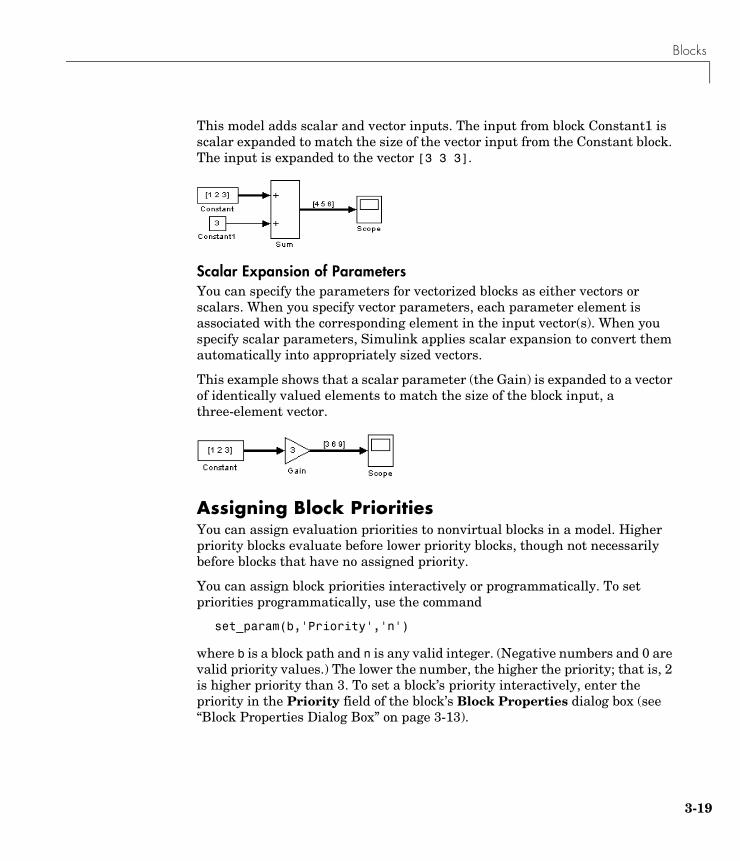
This model adds scalar and vector inputs. The input from block Constant1 isscalar expanded to match the size of the vector input from the Constant block.The input is expanded to the vector [3 3 3].
Scalar Expansion of ParametersYou can specify the parameters for vectorized blocks as either vectors orscalars. When you specify vector parameters, each parameter element isassociated with the corresponding element in the input vector(s). When youspecify scalar parameters, Simulink applies scalar expansion to convert themautomatically into appropriately sized vectors.
This example shows that a scalar parameter (the Gain) is expanded to a vectorof identically valued elements to match the size of the block input, athree-element vector.
Assigning Block PrioritiesYou can assign evaluation priorities to nonvirtual blocks in a model. Higherpriority blocks evaluate before lower priority blocks, though not necessarilybefore blocks that have no assigned priority.
You can assign block priorities interactively or programmatically. To setpriorities programmatically, use the command
set_param(b,'Priority','n')
where b is a block path and n is any valid integer. (Negative numbers and 0 arevalid priority values.) The lower the number, the higher the priority; that is, 2is higher priority than 3. To set a block’s priority interactively, enter thepriority in the Priority field of the block’s Block Properties dialog box (see“Block Properties Dialog Box” on page 3-13).

3 Creating a Model
3-20
Using Drop ShadowsYou can add a drop shadow to a block by selecting the block, then choosingShow Drop Shadow from the Format menu. When you select a block with adrop shadow, the menu item changes to Hide Drop Shadow. The figure belowshows a Subsystem block with a drop shadow.

Libraries
3-21
LibrariesLibraries enable users to copy blocks into their models from external librariesand automatically update the copied blocks when the source blocks change.Using libraries allows users who develop their own block libraries, or who usethose provided by others (such as blocksets), to ensure that their modelsautomatically include the most recent versions of these blocks.
TerminologyIt is important to understand the terminology used with this feature.
Library – A collection of library blocks. A library must be explicitly createdusing New Library from the File menu.
Library block – A block in a library.
Reference block – A copy of a library block.
Link – The connection between the reference block and its library block thatallows Simulink to update the reference block when the library block changes.
Copy – The operation that creates a reference block from either a library blockor another reference block.
This figure illustrates this terminology.
Creating a LibraryTo create a library, select Library from the New submenu of the File menu.Simulink displays a new window, labeled Library: untitled. If an untitledwindow already appears, a sequence number is appended.
You can create a library from the command line using this command.
new_system('newlib', 'Library')
link
copylibraryblock
referenceblock
Library (Source) Model or Library (Destination)

3 Creating a Model
3-22
This command creates a new library named 'newlib'. To display the library,use the open_system command. These commands are described in Chapter 10.
The library must be named (saved) before you can copy blocks from it.
Modifying a LibraryWhen you open a library, it is automatically locked and you cannot modify itscontents. To unlock the library, select Unlock Library from the Edit menu.Closing the library window locks the library.
Copying a Library Block into a ModelYou can copy a block from a library into a model by copying and pasting ordragging the block from the library window to the model window (see “Copyingand Moving Blocks from One Window to Another” on page 3-10) or by draggingthe block from the Library Browser (see “Browsing Block Libraries” on page3-25) into the model window.
When you copy a library block into a model or another library, Simulink createsa link to the library block. The reference block is a copy of the library block. Youcan modify block parameters in the reference block but you cannot mask theblock or, if it is masked, edit the mask. Also, you cannot set callbackparameters for a reference block. If you look under the mask of a referenceblock, Simulink displays the underlying system for the library block.
The library and reference blocks are linked by name; that is, the reference blockis linked to the specific block and library whose names are in effect at the timethe copy is made.
If Simulink is unable to find either the library block or the source library onyour MATLAB path when it attempts to update the reference block, the linkbecomes unresolved. Simulink issues an error message and displays theseblocks using red dashed lines. The error message is
Failed to find block "source-block-name" in library "source-library-name"referenced by block"reference-block-path".

Libraries
3-23
The unresolved reference block is displayed like this (colored red).
To fix a bad link, you must either:
• Delete the unlinked reference block and copy the library block back into yourmodel.
• Add the directory that contains the required library to the MATLAB pathand select Update Diagram from the Edit menu.
• Double-click on the reference block. On the dialog box that appears, correctthe pathname and click on Apply or Close.
All blocks have a LinkStatus parameter that indicates whether the block is areference block. The parameter can have these values:
• 'none' indicates that the block is not a reference block.
• 'resolved' indicates that the block is a reference block and that the link isresolved.
• 'unresolved' indicates that the block is a reference block but that the linkis unresolved.
Updating a Linked BlockSimulink updates out-of-date reference blocks in a model or library at thesetimes:
• When the model or library is loaded
• When you select Update Diagram from the Edit menu or run the simulation
• When you query the LinkStatus parameter of a block using the get_paramcommand (see “Getting Information About Library Blocks” on page 3-24)
• When you use the find_system command
Breaking a Link to a Library BlockYou can break the link between a reference block and its library block to causethe reference block to become a simple copy of the library block, unlinked to the

3 Creating a Model
3-24
library block. Changes to the library block no longer affect the block. Breakinglinks to library blocks enables you to transport a model as a stand-alone model,without the libraries.
To break the link between a reference block and its library block, select theblock, then choose Break Library Link from the Edit menu. You can alsobreak the link between a reference block and its library block from thecommand line by changing the value of the LinkStatus parameter to 'none'using this command.
set_param('refblock', 'LinkStatus', 'none')
You can save a system and break all links between reference blocks and libraryblocks using this command.
save_system('sys', 'newname', 'BreakLinks')
Finding the Library Block for a Reference BlockTo find the source library and block linked to a reference block, select thereference block, then choose Go To Library Link from the Edit menu. If thelibrary is open, Simulink selects the library block (displaying selection handleson the block) and makes the source library the active window. If the library isnot open, Simulink opens it and selects the library block.
Getting Information About Library BlocksUse the libinfo command to get information about reference blocks in asystem. The format for the command is
libdata = libinfo(sys)
where sys is the name of the system. The command returns a structure of sizen-by-1, where n is the number of library blocks in sys. Each element of thestructure has four fields:
• Block, the block path
• Library, the library name
• ReferenceBlock, the reference block path
• LinkStatus, the link status, either 'resolved' or 'unresolved'

Libraries
3-25
Browsing Block LibrariesThe Library Browser lets you quickly locate and copy library blocks into amodel.
Note The Library Browser is available only on Microsoft Windows platforms.
You can locate blocks either by navigating the Library Browser’s library treeor by using the Library Browser’s search facility.
Navigating the Library TreeThe library tree displays a list of all the block libraries installed on the system.You can view or hide the contents of libraries by expanding or collapsing thetree using the mouse or keyboard. To expand/collapse the tree, click the +/-buttons next to library entries or select an entry and press the +/- or right/leftarrow key on your keyboard. Use the up/down arrow keys to move up or downthe tree.
Searching LibrariesTo find a particular block, enter the block’s name in the edit field next to theLibrary Browser’s Find button and then click the Find button.
Opening a LibraryTo open a library, right-click the library’s entry in the browser. Simulinkdisplays an Open Library button. Select the Open Library button to open thelibrary.

3 Creating a Model
3-26
Creating and Opening ModelsTo create a model, select the New button on the Library Browser’s toolbar. Toopen an existing model, select the Open button on the toolbar.
Copying BlocksTo copy a block from the Library Browser into a model, select the block in thebrowser, drag the selected block into the model window, and drop it where youwant to create the copy.
Displaying Help on a BlockTo display help on a block, right-click the block in the Library Browser andselect the button that subsequently pops up.
Pinning the Library Browser To keep the Library Browser above all other windows on your desktop, selectthe PushPin button on the browser’s toolbar.

Lines
3-27
LinesLines carry signals. Each line can carry a scalar or vector signal. A line canconnect the output port of one block with the input port of another block. A linecan also connect the output port of one block with input ports of many blocksby using branch lines.
Drawing a Line Between BlocksTo connect the output port of one block to the input port of another block:
1 Position the cursor over the first block’s output port. It is not necessary toposition the cursor precisely on the port. The cursor shape changes to a crosshair.
2 Press and hold down the mouse button.
3 Drag the pointer to the second block’s input port. You can position the cursoron or near the port, or in the block. If you position the cursor in the block,the line is connected to the closest input port. The cursor shape changes to adouble cross hair.
4 Release the mouse button. Simulink replaces the port symbols by aconnecting line with an arrow showing the direction of the signal flow. Youcan create lines either from output to input, or from input to output. Thearrow is drawn at the appropriate input port, and the signal is the same.
Simulink draws connecting lines using horizontal and vertical line segments.To draw a diagonal line, hold down the Shift key while drawing the line.
3 Creating a Model
3-28
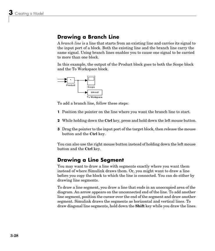
Drawing a Branch LineA branch line is a line that starts from an existing line and carries its signal tothe input port of a block. Both the existing line and the branch line carry thesame signal. Using branch lines enables you to cause one signal to be carriedto more than one block.
In this example, the output of the Product block goes to both the Scope blockand the To Workspace block.
To add a branch line, follow these steps:
1 Position the pointer on the line where you want the branch line to start.
2 While holding down the Ctrl key, press and hold down the left mouse button.
3 Drag the pointer to the input port of the target block, then release the mousebutton and the Ctrl key.
You can also use the right mouse button instead of holding down the left mousebutton and the Ctrl key.
Drawing a Line SegmentYou may want to draw a line with segments exactly where you want theminstead of where Simulink draws them. Or, you might want to draw a linebefore you copy the block to which the line is connected. You can do either bydrawing line segments.
To draw a line segment, you draw a line that ends in an unoccupied area of thediagram. An arrow appears on the unconnected end of the line. To add anotherline segment, position the cursor over the end of the segment and draw anothersegment. Simulink draws the segments as horizontal and vertical lines. Todraw diagonal line segments, hold down the Shift key while you draw the lines.

Lines
3-29
Moving a Line SegmentTo move a line segment, follow these steps:
1 Position the pointer on the segment you want to move.
2 Press and hold down the left mouse button.
3 Drag the pointer to the desired location.
4 Release the mouse button.
You cannot move the segments that are connected directly to block ports.
Dividing a Line into SegmentsYou can divide a line segment into two segments, leaving the ends of the linein their original locations. Simulink creates line segments and a vertex thatjoins them. To divide a line into segments, follow these steps:

3 Creating a Model
3-30
1 Select the line.
2 Position the pointer on the line where you want the vertex.
3 While holding down the Shift key, press and hold down the mouse button.The cursor shape changes to a circle that encloses the new vertex.
4 Drag the pointer to the desired location.
5 Release the mouse button and the Shift key.

Lines
3-31
Moving a Line VertexTo move a vertex of a line, follow these steps:
1 Position the pointer on the vertex, then press and hold down the mousebutton. The cursor changes to a circle that encloses the vertex.
2 Drag the pointer to the desired location.
3 Release the mouse button.
Displaying Line WidthsYou can display the widths of vector lines in a model by turning on Vector LineWidths from the Format menu. Simulink indicates the width of each signal atthe block that originates the signal and the block that receives it. You can causeSimulink to use a thick line to display vector lines by selecting Wide VectorLines from the Format menu.
When you start a simulation or update the diagram and Simulink detects amismatch of input and output ports, it displays an error message and showsline widths in the model.
Inserting Blocks in a LineYou can insert a block in a line by dropping the block on the line. Simulinkinserts the block for you at the point where you drop the block. The block thatyou insert can have only one input and one output.

3 Creating a Model
3-32
To insert a block in a line:
1 Position the pointer over the block and press the left mouse button.
2 Drag the block over the line in which you want to insert the block.
3 Release the mouse button to drop the block on the line. Simulink inserts theblock where you dropped it.
Signal LabelsYou can label signals to annotate your model. Labels can appear above or belowhorizontal lines or line segments, and left or right of vertical lines or linesegments. Labels can appear at either end, at the center, or in any combinationof these locations.
Lines
3-33
Using Signal LabelsTo create a signal label, double-click on the line segment and type the label atthe insertion point. When you click on another part of the model, the label fixesits location.
Note When you create a signal label, take care to double-click on the line. Ifyou click in an unoccupied area close to the line, you will create a modelannotation instead.
To move a signal label, drag the label to a new location on the line. When yourelease the mouse button, the label fixes its position near the line.
To copy a signal label, hold down the Ctrl key while dragging the label toanother location on the line. When you release the mouse button, the labelappears in both the original and the new locations.
To edit a signal label, select it:
• To replace the label, click on the label, then double-click or drag the cursorto select the entire label. Then, enter the new label.
• To insert characters, click between two characters to position the insertionpoint, then insert text.
• To replace characters, drag the mouse to select a range of text to replace,then enter the new text.
To delete all occurrences of a signal label, delete all the characters in the label.When you click outside the label, the labels are deleted. To delete a singleoccurrence of the label, hold down the Shift key while you select the label, thenpress the Delete or Backspace key.
To change the font of a signal label, select the signal, choose Font from theFormat menu, then select a font from the Set Font dialog box.
Signal Label PropagationSignal label propagation is the automatic labeling of a line emitting from aconnection block. Blocks that support signal label propagation are the Demux,Enable, From, Inport, Mux, Selector, and Subsystem blocks. The labeled signal

3 Creating a Model
3-34
must be on a line feeding a connecting block and the propagated signal must beon a line coming from the same connecting block or one associated with it.
To propagate a signal label, create a signal label starting with the “<” characteron the output of one of the listed connection blocks. When you run thesimulation or update the diagram, the actual signal label appears, enclosedwithin angle brackets. The actual signal label is obtained by tracing backthrough the connection blocks until a signal label is encountered.
This example shows a model with a signal label and the propagated label bothbefore and after updating the block diagram. In the first figure, the signalentering the Goto block is labeled label and the signal leaving the associatedFrom block is labeled with a single <. The second figure shows the same modelafter choosing Update Diagram from the Edit menu.
In the next example, the propagated signal label shows the contents of a vectorsignal. This figure shows the label only after updating the diagram.
Setting Signal PropertiesSignals have properties. Use Simulink’s Signal Properties dialog box to viewor set a signal’s properties. To display the dialog box, select the line that carriesthe signal and choose Signal Properties from the Simulink Edit menu.
The signal label and propagated label before updating the diagram.
The same signal labels after updating the diagram.
1
2

Lines
3-35
Signal Properties Dialog BoxThe Signal Properties dialog box allows you to view and edit signal properties.
The dialog box includes the following controls.
Signal NameName of signal.
DescriptionEnter a description of the signal in this field.
Document LinkEnter a MATLAB expression in the field that displays documentation for thesignal. To display the documentation, click the field’s label (that is, “DocumentLink”). For example, entering the expression
web(['file:///' which('foo_signal.html')])
in the field causes MATLAB’s default Web browser to displayfoo_signal.html when you click the field’s label.
Displayable (Test Point)Check this option to indicate that the signal can be displayed duringsimulation.
3 Creating a Model
3-36
Note The next two controls are used to set properties used by the Real-TimeWorkshop to generate code from the model. You can ignore them if you do notplan to generate code from the model.
RTW storage classSelect the storage class of this signal from the list. See the Real-Time WorkshopUser’s Guide for an explanation of the listed options.
RTW storage type qualifierSelect the storage type of this signal from the list. See the Real-Time WorkshopUser’s Guide for more information.

Annotations
3-37
AnnotationsAnnotations provide textual information about a model. You can add anannotation to any unoccupied area of your block diagram.
To create a model annotation, double-click on an unoccupied area of the blockdiagram. A small rectangle appears and the cursor changes to an insertionpoint. Start typing the annotation contents. Each line is centered within therectangle that surrounds the annotation.
To move an annotation, drag it to a new location.
To edit an annotation, select it:
• To replace the annotation on a Microsoft Windows or UNIX system, click onthe annotation, then double-click or drag the cursor to select it. Then, enterthe new annotation.
• To insert characters, click between two characters to position the insertionpoint, then insert text.
• To replace characters, drag the mouse to select a range of text to replace,then enter the new text.
To delete an annotation, hold down the Shift key while you select theannotation, then press the Delete or Backspace key.
To change the font of all or part of an annotation, select the text in theannotation you want to change, then choose Font from the Format menu.Select a font and size from the dialog box.
Annotations

3 Creating a Model
3-38
Working with Data TypesThe term data type refers to the way in which a computer represents numbersin memory. A data type determines the amount of storage allocated to anumber, the method used to encode the number’s value as a pattern of binarydigits, and the operations available for manipulating the type. Most computersprovide a choice of data types for representing numbers, each with specificadvantages in the areas of precision, dynamic range, performance, and memoryusage. To enable you to take advantage of data typing to optimize theperformance of MATLAB programs, MATLAB allows you to specify the datatype of MATLAB variables. Simulink builds on this capability by allowing youto specify the data types of Simulink signals and block parameters.
The ability to specify the data types of a model’s signals and block parametersis particularly useful in real-time control applications. For example, it allows aSimulink model to specify the optimal data types to use to represent signalsand block parameters in code generated from a model by automaticcode-generation tools, such as the Real-Time Workshop available from TheMathWorks. By choosing the most appropriate data types for your model’ssignals and parameters, you can dramatically increase the performance anddecrease the size of the code generated from the model.
Simulink performs extensive checking before and during a simulation toensure that your model is typesafe, that is, that code generated from the modelwill not overflow or underflow and thus produce incorrect results. Simulinkmodels that use Simulink’s default data type (double) are inherently typesafe.Thus, if you never plan to generate code from your model or use a nondefaultdata type in your models, you can skip the remainder of this section.
On the other hand, if you plan to generate code from your models and usenondefault data types, read the remainder of this section carefully, especiallythe section on data type rules (see “Data Typing Rules” on page 3-44). In thatway, you can avoid introducing data type errors that prevent your model fromrunning to completion or simulating at all.
Data Types Supported by SimulinkSimulink supports all built-in MATLAB data types. The term built-in data typerefers to data types defined by MATLAB itself as opposed to data types definedby MATLAB users. Unless otherwise specified, the term data type in the
Working with Data Types
3-39
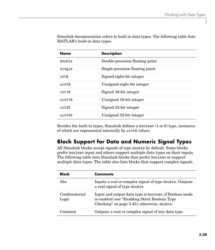
Simulink documentation refers to built-in data types. The following table listsMATLAB’s built-in data types.
Besides the built-in types, Simulink defines a boolean (1 or 0) type, instancesof which are represented internally by uint8 values.
Block Support for Data and Numeric Signal TypesAll Simulink blocks accept signals of type double by default. Some blocksprefer boolean input and others support multiple data types on their inputs.The following table lists Simulink blocks that prefer boolean or supportmultiple data types. The table also lists blocks that support complex signals.
Name Description
double Double-precision floating point
single Single-precision floating point
int8 Signed eight-bit integer
uint8 Unsigned eight-bit integer
int16 Signed 16-bit integer
uint16 Unsigned 16-bit integer
int32 Signed 32-bit integer
uint32 Unsigned 32-bit integer
Block Comments
Abs Inputs a real or complex signal of type double. Outputsa real signal of type double.
CombinatorialLogic
Input and output data type is boolean, if Boolean modeis enabled (see “Enabling Strict Boolean TypeChecking” on page 3-45); otherwise, double.
Constant Outputs a real or complex signal of any data type.

3 Creating a Model
3-40
Data TypeConversion
Inputs and outputs any real or complex data type.
Demux Accepts mixed-type signal vectors.
Display Accepts signals of any complex or real data type.
Dot Product Inputs and outputs real or complex values of typedouble.
Enable The corresponding subsystem enable port acceptssignals of type boolean or double.
From Outputs the data type (or types) of the signal connectedto the corresponding Goto block.
FromWorkspace
Outputs type of corresponding workspace values.
Gain Input can be a real- or complex-valued signal or vectorof any data type except boolean.
Goto Input can be of any type.
Ground Outputs a 0 signal of the same type as the port to whichit is connected.
Hit Crossing Inputs a double signal. Outputs boolean, if Booleanmode is enabled (see “Enabling Strict Boolean TypeChecking” on page 3-45); otherwise, double.
Inport An inport accepts real- or complex-valued signals of anydata type. The elements of an input signal vector mustbe of the same type if the inport is a root-level inport orthe inport is directly connected to an outport of thesame subsystem.
Integrator An Integrator block accepts and outputs signals of typedouble on its data ports. Its external reset port acceptssignals of type double or boolean.
Block Comments

Working with Data Types
3-41
LogicalOperator
Inputs and outputs real signals of type boolean, ifBoolean mode is enabled (see “Enabling Strict BooleanType Checking” on page 3-45); otherwise, real signals oftype double.
Manual Switch Accepts real- or complex-valued signals of any type. Allinputs must have the same signal and data type.
Math Function Inputs and outputs real or complex values of typedouble.
MATLABFunction
Inputs and outputs real or complex values of typedouble.
Memory Inputs real or complex signals of any data type.
Merge Inputs and outputs any real or complex data type.
MultiportSwitch
The control input of a Multiport Switch block accepts areal-valued signal of any type except boolean. Theother inputs accept real- or complex-valued inputs ofany type. All inputs must of the same data and numerictype. The block outputs the type of signal on its inputs.
Mux Accepts any supported Simulink data type, includingmixed-type vectors, on each input.
Out Accepts any Simulink data type as input. Acceptsmixed-type vectors as input, if the outport is in asubsystem and no initial condition is specified.
Product Accepts real- or complex-valued signals of any datatype except boolean. All inputs must be of the samedata type.
RelationalOperator
Accepts any supported data type as inputs. Both inputsmust be of the same type. Outputs boolean, if Booleanmode is enabled (see “Enabling Strict Boolean TypeChecking” on page 3-45); otherwise, double.
Block Comments

3 Creating a Model
3-42
See Chapter 8, “Block Reference” for more information on the data typessupported by specific blocks for parameter and input and output values. If thedocumentation for a block does not specify a data type, the block inputs oroutputs only data of type double.
RoundingFunction
Accepts and outputs real or complex values of typedouble.
Scope Accepts real or complex signals of any data type.
Selector Outputs the data types of the selected input signals.
Sum Accepts any Simulink data type as input. All inputsmust be of the same type. Outputs the same type as theinput.
Switch Accepts real- or complex-valued signals of any datatype as switched inputs (inputs 1 and 3). Both switchedinputs must be of the same type. The block outputsignal has the data type of the input. The data type ofthe threshold input must be boolean or double.
Terminator Accepts any Simulink type.
To Workspace Accepts any Simulink data type as input.
Trigger The corresponding subsystem control port acceptssignals of type boolean or double.
TrigonometricFunction
Inputs and outputs real- or complex-valued signals oftype double.
Unit Delay Accepts and outputs real- or complex-valued signals ofany data type.
Width Accepts real- or complex-valued signals of any datatype, including mixed-type signal vectors.
Zero-Order Hold Accepts any Simulink data type as input.
Block Comments
Working with Data Types
3-43
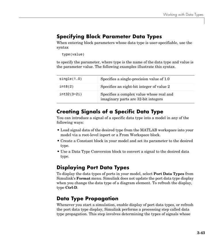
Specifying Block Parameter Data TypesWhen entering block parameters whose data type is user-specifiable, use thesyntax
type(value)
to specify the parameter, where type is the name of the data type and value isthe parameter value. The following examples illustrate this syntax.
Creating Signals of a Specific Data TypeYou can introduce a signal of a specific data type into a model in any of thefollowing ways:
• Load signal data of the desired type from the MATLAB workspace into yourmodel via a root-level inport or a From Workspace block.
• Create a Constant block in your model and set its parameter to the desiredtype.
• Use a Data Type Conversion block to convert a signal to the desired datatype.
Displaying Port Data TypesTo display the data types of ports in your model, select Port Data Types fromSimulink’s Format menu. Simulink does not update the port data type displaywhen you change the data type of a diagram element. To refresh the display,type Ctrl-D.
Data Type PropagationWhenever you start a simulation, enable display of port data types, or refreshthe port data type display, Simulink performs a processing step called datatype propagation. This step involves determining the types of signals whose
single(1.0) Specifies a single-precision value of 1.0
int8(2) Specifies an eight-bit integer of value 2
int32(3+2i) Specifies a complex value whose real andimaginary parts are 32-bit integers

3 Creating a Model
3-44
type is not otherwise specified and checking the types of signals and input portsto ensure that they do not conflict. If type conflicts arise, Simulink displays anerror dialog that specifies the signal and port whose data types conflict.Simulink also highlights the signal path that creates the type conflict.
Note You can insert typecasting (data type conversion) blocks in your modelto resolve type conflicts. See“Typecasting Signals” on page 3-45 for moreinformation.
Data Typing RulesObserving the following rules will help you to create models that are typesafeand therefore execute without error:
• Signal data types generally do not affect parameter data types, and viceversa.
A significant exception to this rule is the Constant block whose output datatype is determined by the data type of its parameter.
• If the output of a block is a function of an input and a parameter and theinput and parameter differ in type, Simulink converts the parameter to theinput type before computing the output.
See “Typecasting Parameters” on page 3-45 for more information.
• In general, a block outputs the data type that appears at its inputs.
Significant exceptions include constant blocks and data type conversionblocks whose output data types are determined by block parameters.
• Virtual blocks accept signals of any type on their inputs.
Examples of virtual blocks include Mux and Demux blocks andunconditionally executed subsystems.
• The elements of a signal vector connected to a port of a nonvirtual block mustbe of the same data type.
• The signals connected to the input data ports of a nonvirtual block cannotdiffer in type.
• Control ports (for example, Enable and Trigger ports) accept boolean ordouble signals.

Working with Data Types
3-45
• Solver blocks accept only double signals.
• Connecting a nondouble signal to a block disables zero-crossing detection forthat block.
Enabling Strict Boolean Type CheckingBy default, Simulink detects but does not signal an error when it detects thatdouble signals are connected to block that prefer boolean input. This ensurescompatibility with models created by earlier versions of Simulink that supportonly double data type. You can enable strict boolean type checking byunchecking the Relax boolean type checking option on the Diagnostics pageof the Simulation Parameters dialog box (see “The Diagnostics Page” on page4-24).
Typecasting SignalsSimulink signals an error whenever it detects that a signal is connected to ablock that does not accept the signal’s data type. If you want to create such aconnection, you must explicitly typecast (convert) the signal to a type that theblock does accept. You can use Simulink’s Data Type Conversion block toperform such conversions (see Data Type Conversion on page 8-41).
Typecasting ParametersIn general, during simulation, Simulink silently converts parameter data typesto signal data types (if they differ) when computing block outputs that are afunction of an input signal and a parameter. The following exceptions occur tothis rule:
• If the signal data type cannot represent the parameter value, Simulink haltsthe simulation and signals an error.
Consider, for example, the following model.
This model uses a Gain block to amplify a constant input signal. Computingthe output of the Gain block requires computing the product of the input

3 Creating a Model
3-46
signal and the gain. Such a computation requires that the two values be ofthe same data type. However, in this case, the data type of the signal, uint8(unsigned 8-bit word), differs from the data type of the gain parameter, int32(signed 32-bit integer). Thus computing the output of the gain block entailsa type conversion.
When making such conversions, Simulink always casts the parameter typeto the signal type. Thus, in this case, Simulink must convert the Gain block’sgain value to the data type of the input signal. Simulink can make thisconversion only if the input signal’s data type (uint8) can represent the gain.In this case, Simulink can make the conversion because the gain is 255,which is within the range of the uint8 data type (0 to 255). Thus, this modelsimulates without error. However, if the gain were slightly larger (forexample, 256), Simulink would signal an out-of-range error if you attemptedto simulate the model.
• If the signal data type can represent the parameter value but only at reducedprecision, Simulink issues a warning message and continues the simulation.
Consider, for example, the following model.
In this example, the signal type accommodates only integer values while thegain value has a fractional component. Simulating this model causesSimulink to truncate the gain to the nearest integral value (2) and issue aloss-of-precision warning. On the other hand, if the gain were 2.0, Simulinkwould simulate the model without complaint because in this case theconversion entails no loss of precision.
Note Conversion of an int32 parameter to a float or double can entail aloss of precision. The loss can be severe if the magnitude of the parametervalue is large. If an int32 parameter conversion does entail a loss of precision,Simulink issues a warning message.
Working with Complex Signals
3-47
Working with Complex SignalsBy default, the values of Simulink signals are real numbers. However, modelscan create and manipulates signals that have complex numbers as values.
You can introduce a complex-valued signal into a model in any of the followingways:
• Load complex-valued signal data from the MATLAB workspace into themodel via a root-level inport.
• Create a Constant block in your model and set its value to a complex number.
• Create real signals corresponding to the real and imaginary parts of acomplex signal and then combine the parts into a complex signal, usingReal-Imag to Complex conversion block.
You can manipulate complex signals via blocks that accept them. MostSimulink blocks accept complex signals as input. If you are not sure whether ablock accepts complex signals, refer to the documentation for the block inChapter 8, “Block Reference.”

3 Creating a Model
3-48
Summary of Mouse and Keyboard ActionsThese tables summarize the use of the mouse and keyboard to manipulateblocks, lines, and signal labels. LMB means press the left mouse button; CMB,the center mouse button; and RMB, the right mouse button.
The first table lists mouse and keyboard actions that apply to blocks.
The next table lists mouse and keyboard actions that apply to lines.
Table 3-2: Manipulating Blocks
Task Microsoft Windows UNIX
Select one block LMB LMB
Select multipleblocks
Shift + LMB Shift + LMB; or CMBalone
Copy block fromanother window
Drag block Drag block
Move block Drag block Drag block
Duplicate block Ctrl + LMB and drag;or RMB and drag
Ctrl + LMB and drag;or RMB and drag
Connect blocks LMB LMB
Disconnect block Shift + drag block Shift + drag block; orCMB and drag
Table 3-3: Manipulating Lines
Task Microsoft Windows UNIX
Select one line LMB LMB
Select multiple lines Shift + LMB Shift + LMB; or CMBalone
Draw branch line Ctrl + drag line; orRMB and drag line
Ctrl + drag line; orRMB + drag line

Summary of Mouse and Keyboard Actions
3-49
The next table lists mouse and keyboard actions that apply to signal labels.
The next table lists mouse and keyboard actions that apply to annotations.
Route lines aroundblocks
Shift + draw linesegments
Shift + draw linesegments; or CMB anddraw segments
Move line segment Drag segment Drag segment
Move vertex Drag vertex Drag vertex
Create linesegments
Shift + drag line Shift + drag line; orCMB + drag line
Table 3-4: Manipulating Signal Labels
Action Microsoft Windows UNIX
Create signal label Double-click on line,then type label
Double-click on line,then type label
Copy signal label Ctrl + drag label Ctrl + drag label
Move signal label Drag label Drag label
Edit signal label Click in label, then edit Click in label, then edit
Delete signal label Shift + click on label,then press Delete
Shift + click on label,then press Delete
Table 3-5: Manipulating Annotations
Action Microsoft Windows UNIX
Create annotation Double-click indiagram, then type text
Double-click indiagram, then type text
Copy annotation Ctrl + drag label Ctrl + drag label
Table 3-3: Manipulating Lines (Continued)
Task Microsoft Windows UNIX

3 Creating a Model
3-50
Move annotation Drag label Drag label
Edit annotation Click in text, then edit Click in text, then edit
Delete annotation Shift + selectannotation, then pressDelete
Shift + selectannotation, then pressDelete
Table 3-5: Manipulating Annotations (Continued)
Action Microsoft Windows UNIX

Creating Subsystems
3-51
Creating SubsystemsAs your model increases in size and complexity, you can simplify it by groupingblocks into subsystems. Using subsystems has these advantages:
• It helps reduce the number of blocks displayed in your model window.
• It allows you to keep functionally related blocks together.
• It enables you to establish a hierarchical block diagram, where a Subsystemblock is on one layer and the blocks that make up the subsystem are onanother.
You can create a subsystem in two ways:
• Add a Subsystem block to your model, then open that block and add theblocks it contains to the subsystem window.
• Add the blocks that make up the subsystem, then group those blocks into asubsystem.
Creating a Subsystem by Adding the Subsystem BlockTo create a subsystem before adding the blocks it contains, add a Subsystemblock to the model, then add the blocks that make up the subsystem:
1 Copy the Subsystem block from the Signals & Systems library into yourmodel.
2 Open the Subsystem block by double-clicking on it.
3 In the empty Subsystem window, create the subsystem. Use Inport blocks torepresent input from outside the subsystem and Outport blocks to representexternal output. For example, the subsystem below includes a Sum blockand Inport and Outport blocks to represent input to and output from thesubsystem:

3 Creating a Model
3-52
Creating a Subsystem by Grouping Existing BlocksIf your model already contains the blocks you want to convert to a subsystem,you can create the subsystem by grouping those blocks:
1 Enclose the blocks and connecting lines that you want to include in thesubsystem within a bounding box. You cannot specify the blocks to begrouped by selecting them individually or by using the Select All command.For more information, see “Selecting Multiple Objects Using a BoundingBox” on page 3–7.
For example, this figure shows a model that represents a counter. The Sumand Unit Delay blocks are selected within a bounding box.
When you release the mouse button, the two blocks and all the connectinglines are selected.
2 Choose Create Subsystem from the Edit menu. Simulink replaces theselected blocks with a Subsystem block. This figure shows the model afterchoosing the Create Subsystem command (and resizing the Subsystemblock so the port labels are readable).
If you open the Subsystem block, Simulink displays the underlying system, asshown below. Notice that Simulink adds Inport and Outport blocks torepresent input from and output to blocks outside the subsystem.

Creating Subsystems
3-53
As with all blocks, you can change the name of the Subsystem block. Also, youcan customize the icon and dialog box for the block using the masking feature,described in Chapter 6.
Labeling Subsystem PortsSimulink labels ports on a Subsystem block. The labels are the names of Inportand Outport blocks that connect the subsystem to blocks outside the subsystemthrough these ports.
You can hide the port labels by selecting the Subsystem block, then choosingHide Port Labels from the Format menu. You can also hide one or more portlabels by selecting the appropriate Inport or Outport block in the subsystemand choosing Hide Name from the Format menu.
This figure shows two models. The subsystem on the left contains two Inportblocks and one Outport block. The Subsystem block on the right shows thelabeled ports.
Using Callback RoutinesYou can define MATLAB expressions that execute when the block diagram ora block is acted upon in a particular way. These expressions, called callbackroutines, are associated with block or model parameters. For example, thecallback associated with a block’s OpenFcn parameter is executed when themodel user double-clicks on that block’s name or path changes.
To define callback routines and associate them with parameters, use theset_param command (see set_param on page 10-24).
For example, this command evaluates the variable testvar when the userdouble-clicks on the Test block in mymodel:
set_param('mymodel/Test', 'OpenFcn', testvar)
You can examine the clutch system (clutch.mdl) for routines associated withmany model callbacks.
3 Creating a Model
3-54
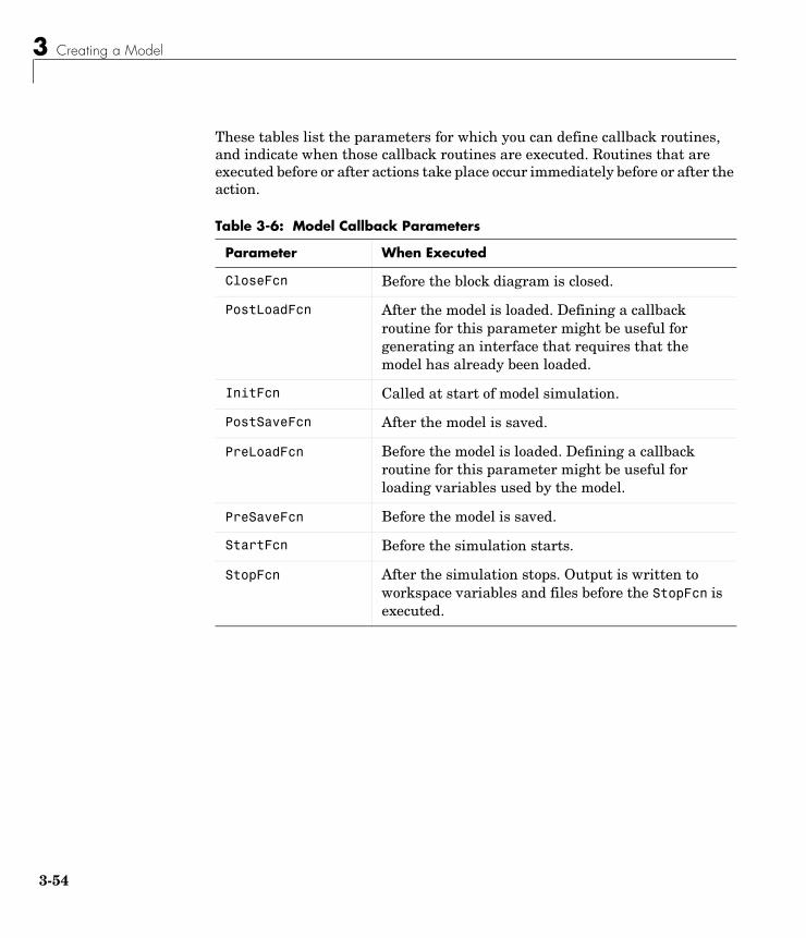
These tables list the parameters for which you can define callback routines,and indicate when those callback routines are executed. Routines that areexecuted before or after actions take place occur immediately before or after theaction.
Table 3-6: Model Callback Parameters
Parameter When Executed
CloseFcn Before the block diagram is closed.
PostLoadFcn After the model is loaded. Defining a callbackroutine for this parameter might be useful forgenerating an interface that requires that themodel has already been loaded.
InitFcn Called at start of model simulation.
PostSaveFcn After the model is saved.
PreLoadFcn Before the model is loaded. Defining a callbackroutine for this parameter might be useful forloading variables used by the model.
PreSaveFcn Before the model is saved.
StartFcn Before the simulation starts.
StopFcn After the simulation stops. Output is written toworkspace variables and files before the StopFcn isexecuted.

Creating Subsystems
3-55
Table 3-7: Block Callback Parameters
Parameter When Executed
CloseFcn When the block is closed using the close_systemcommand.
CopyFcn After a block is copied. The callback is recursive forSubsystem blocks (that is, if you copy a Subsystemblock that contains a block for which the CopyFcnparameter is defined, the routine is also executed).The routine is also executed if an add_blockcommand is used to copy the block.
DeleteFcn Before a block is deleted. This callback is recursivefor Subsystem blocks.
DestroyFcn When block has been destroyed.
InitFcn Before the block diagram is compiled and beforeblock parameters are evaluated.
LoadFcn After the block diagram is loaded. This callback isrecursive for Subsystem blocks.
ModelCloseFcn Before the block diagram is closed. This callback isrecursive for Subsystem blocks.
MoveFcn When block is moved or resized.
NameChangeFcn After a block’s name and/or path changes. When aSubsystem block’s path is changed, it recursivelycalls this function for all blocks it contains aftercalling its own NameChangeFcn routine.

3 Creating a Model
3-56
OpenFcn When the block is opened. This parameter isgenerally used with Subsystem blocks. The routineis executed when you double-click on the block orwhen an open_system command is called with theblock as an argument. The OpenFcn parameteroverrides the normal behavior associated withopening a block, which is to display the block’sdialog box or to open the subsystem.
ParentCloseFcn Before closing a subsystem containing the block orwhen the block is made part of a new subsystemusing the new_system command (see new_systemon page 10-19).
PreSaveFcn Before the block diagram is saved. This callback isrecursive for Subsystem blocks.
PostSaveFcn After the block diagram is saved. This callback isrecursive for Subsystem blocks.
StartFcn After the block diagram is compiled and before thesimulation starts.
StopFcn At any termination of the simulation.
UndoDeleteFcn When a block delete is undone.
Table 3-7: Block Callback Parameters (Continued)
Parameter When Executed
Tips for Building Models
3-57
Tips for Building ModelsHere are some model-building hints you might find useful:
• Memory issues
In general, the more memory, the better Simulink performs.
• Using hierarchy
More complex models often benefit from adding the hierarchy of subsystemsto the model. Grouping blocks simplifies the top level of the model and canmake it easier to read and understand the model. For more information, see“Creating Subsystems” on page 3–51. The Model Browser (see “The ModelBrowser” on page 3-66) provides useful information about complex models.
• Cleaning up models
Well organized and documented models are easier to read and understand.Signal labels and model annotations can help describe what is happening ina model. For more information, see “Signal Labels” on page 3–32 and“Annotations” on page 3–37.
• Modeling strategies
If several of your models tend to use the same blocks, you might find it easierto save these blocks in a model. Then, when you build new models, just openthis model and copy the commonly used blocks from it. You can create a blocklibrary by placing a collection of blocks into a system and saving the system.You can then access the system by typing its name in the MATLAB commandwindow.
Generally, when building a model, design it first on paper, then build it usingthe computer. Then, when you start putting the blocks together into a model,add the blocks to the model window before adding the lines that connectthem. This way, you can reduce how often you need to open block libraries.

3 Creating a Model
3-58
Modeling EquationsOne of the most confusing issues for new Simulink users is how to modelequations. Here are some examples that may improve your understanding ofhow to model equations.
Converting Celsius to FahrenheitTo model the equation that converts Celsius temperature to Fahrenheit:
TF = 9/5(TC) + 32
First, consider the blocks needed to build the model:
• A Ramp block to input the temperature signal, from the Sources library
• A Constant block, to define a constant of 32, also from the Sources library
• A Gain block, to multiply the input signal by 9/5, from the Math library
• A Sum block, to add the two quantities, also from the Math library
• A Scope block to display the output, from the Sinks library
Next, gather the blocks into your model window.
Assign parameter values to the Gain and Constant blocks by opening(double-clicking on) each block and entering the appropriate value. Then, clickon the Close button to apply the value and close the dialog box.
Now, connect the blocks.

Modeling Equations
3-59
The Ramp block inputs Celsius temperature. Open that block and change theInitial output parameter to 0. The Gain block multiplies that temperature bythe constant 9/5. The Sum block adds the value 32 to the result and outputs theFahrenheit temperature.
Open the Scope block to view the output. Now, choose Start from theSimulation menu to run the simulation. The simulation will run for 10seconds.
Modeling a Simple Continuous SystemTo model the differential equation
where u(t) is a square wave with an amplitude of 1 and a frequency of 1rad/sec. The Integrator block integrates its input, x′, to produce x. Other blocksneeded in this model include a Gain block and a Sum block. To generate asquare wave, use a Signal Generator block and select the Square Wave formbut change the default units to radians/sec. Again, view the output using aScope block. Gather the blocks and define the gain.
In this model, to reverse the direction of the Gain block, select the block, thenuse the Flip Block command from the Format menu. Also, to create the branchline from the output of the Integrator block to the Gain block, hold down theCtrl key while drawing the line. For more information, see “Drawing a BranchLine” on page 3–28. Now you can connect all the blocks.
An important concept in this model is the loop that includes the Sum block, theIntegrator block, and the Gain block. In this equation, x is the output of theIntegrator block. It is also the input to the blocks that compute x′, on which itis based. This relationship is implemented using a loop.
x′ t( ) 2x t( )– u t( )+=

3 Creating a Model
3-60
The Scope displays x at each time step. For a simulation lasting 10 seconds, theoutput looks like this.
The equation you modeled in this example can also be expressed as a transferfunction. The model uses the Transfer Fcn block, which accepts u as input andoutputs x. So, the block implements x/u. If you substitute sx for x′ in theequation above.
Solving for x gives
Or,
The Transfer Fcn block uses parameters to specify the numerator anddenominator coefficients. In this case, the numerator is 1 and the denominatoris s+2. Specify both terms as vectors of coefficients of successively decreasingpowers of s. In this case the numerator is [1] (or just 1) and the denominatoris [1 2]. The model now becomes quite simple:
The results of this simulation are identical to those of the previous model.
sx 2x– u+=
x u s 2+( )⁄=
x u⁄ 1 s 2+( )⁄=
Saving a Model
3-61
Saving a ModelYou can save a model by choosing either the Save or Save As command fromthe File menu. Simulink saves the model by generating a specially formattedfile called the model file (with the .mdl extension) that contains the blockdiagram and block properties. The format of the model file is described inAppendix B.
If you are saving a model for the first time, use the Save command to providea name and location to the model file. Model file names must start with a letterand can contain no more than 31 letters, numbers, and underscores.
If you are saving a model whose model file was previously saved, use the Savecommand to replace the file’s contents or the Save As command to save themodel with a new name or location.
Simulink follows this procedure while saving a model:
1 If the mdl file for the model already exists, it is renamed as a temporary file.
2 Simulink executes all block PreSaveFcn callback routines, then executes theblock diagram’s PreSaveFcn callback routine.
3 Simulink writes the model file to a new file using the same name and anextension of mdl.
4 Simulink executes all block PostSaveFcn callback routines, then executesthe block diagram’s PostSaveFcn callback routine.
5 Simulink deletes the temporary file.
If an error occurs during this process, Simulink renames the temporary file tothe name of the original model file, writes the current version of the model to afile with an .err extension, and issues an error message. Simulink performssteps 2 through 4 even if an error occurs in an earlier step.

3 Creating a Model
3-62
Printing a Block DiagramYou can print a block diagram by selecting Print from the File menu (on aMicrosoft Windows system) or by using the print command in the MATLABcommand window (on all platforms).
On a Microsoft Windows system, the Print menu item prints the block diagramin the current window.
Print Dialog BoxWhen you select the Print menu item, the Print dialog box appears. The Printdialog box enables you to selectively print systems within your model. Usingthe dialog box, you can:
• Print the current system only
• Print the current system and all systems above it in the model hierarchy
• Print the current system and all systems below it in the model hierarchy,with the option of looking into the contents of masked and library blocks
• Print all systems in the model, with the option of looking into the contents ofmasked and library blocks
• Print an overlay frame on each diagram
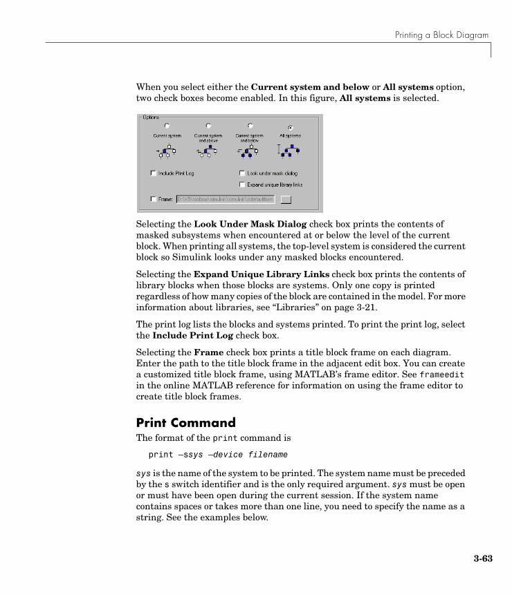
The portion of the Print dialog box that supports selective printing is similaron supported platforms. This figure shows how it looks on a Microsoft Windowssystem. In this figure, only the current system is to be printed.
Printing a Block Diagram
3-63
When you select either the Current system and below or All systems option,two check boxes become enabled. In this figure, All systems is selected.
Selecting the Look Under Mask Dialog check box prints the contents ofmasked subsystems when encountered at or below the level of the currentblock. When printing all systems, the top-level system is considered the currentblock so Simulink looks under any masked blocks encountered.
Selecting the Expand Unique Library Links check box prints the contents oflibrary blocks when those blocks are systems. Only one copy is printedregardless of how many copies of the block are contained in the model. For moreinformation about libraries, see “Libraries” on page 3-21.
The print log lists the blocks and systems printed. To print the print log, selectthe Include Print Log check box.
Selecting the Frame check box prints a title block frame on each diagram.Enter the path to the title block frame in the adjacent edit box. You can createa customized title block frame, using MATLAB’s frame editor. See frameeditin the online MATLAB reference for information on using the frame editor tocreate title block frames.
Print CommandThe format of the print command is
print –ssys –device filename
sys is the name of the system to be printed. The system name must be precededby the s switch identifier and is the only required argument. sys must be openor must have been open during the current session. If the system namecontains spaces or takes more than one line, you need to specify the name as astring. See the examples below.

3 Creating a Model
3-64
device specifies a device type. For a list and description of device types, seeUsing MATLAB Graphics.
filename is the PostScript file to which the output is saved. If filename exists,it is replaced. If filename does not include an extension, an appropriate one isappended.
For example, this command prints a system named untitled.
print –suntitled
This command prints the contents of a subsystem named Sub1 in the currentsystem.
print –sSub1
This command prints the contents of a subsystem named Requisite Friction.
print (['–sRequisite Friction'])
The next example prints a system named Friction Model, a subsystem whosename appears on two lines. The first command assigns the newline characterto a variable; the second prints the system.
cr = sprintf('\n');print (['–sFriction' cr 'Model'])
Specifying Paper Size and OrientationSimulink lets you specify the type and orientation of the paper used to print amodel diagram. You can do this on all platforms by setting the model’sPaperType and PaperOrientation properties, respectively (see “ModelParameters” on page A-3), using the set_param command. You can set thepaper orientation alone, using MATLAB’s orient command. On Windows, thePrint dialog box lets you set the page type and orientation properties as well.
Positioning and Sizing a DiagramYou can use a model’s PaperPositionMode and PaperPosition parameters toposition and size the model’s diagram on the printed page. The value of thePaperPosition parameter is a vector of form [left bottom width height].The first two elements specify the bottom left corner of a rectangular area onthe page, measured from the page’s bottom left corner. The last two elementsspecify the width and height of the rectangle. When the model’s

Printing a Block Diagram
3-65
PaperPositionMode is manual, Simulink positions (and scales, if necessary)the model’s diagram to fit inside the specified print rectangle. For example, thefollowing commands
vdpset_param(‘vdp’, ‘PaperType’, ‘usletter’)set_param('vdp', 'PaperOrientation', 'landscape')set_param(‘vdp’, ‘PaperPositionMode’, ‘manual’)set_param(‘vdp’, ‘PaperPosition’, [0.5 0.5 4 4])print -svdp
print the block diagram of the vdp sample model in the lower left corner of aU.S. letter-size page in landscape orientation.
If PaperPositionMode is auto, Simulink centers the model diagram on theprinted page, scaling the diagram, if necessary, to fit the page.

3 Creating a Model
3-66
The Model BrowserThe Model Browser enables you to:
• Navigate a model hierarchically
• Open systems in a model directly
• Determine the blocks contained in a model
The browser operates differently on Microsoft Windows and UNIX platforms.
Using the Model Browser on WindowsTo display the Model Browser pane, select Model Browser from the SimulinkView menu. The model window splits into two panes. The left pane displays thebrowser, a tree-structured view of the block diagram displayed in the rightpane.
Each entry in the tree view corresponds to a subsystem in the model. You canexpand/collapse the tree by clicking on the +/- boxes beside each subsystem, orby pressing the left/right arrow or +/- keys on your numeric keypad. You canmove up/down the tree by pressing the up/down arrow on your keypad. Clickon any subsystem to display its contents in the diagram view. To open a newwindow on a subsystem, double click the subsystem in the diagram view.
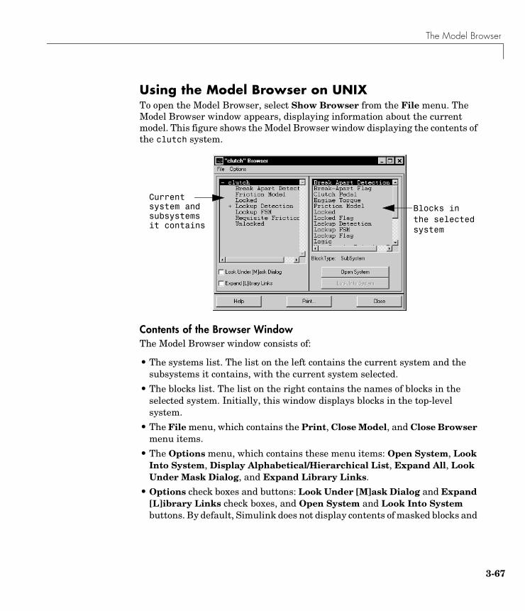
The Model Browser
3-67
Using the Model Browser on UNIXTo open the Model Browser, select Show Browser from the File menu. TheModel Browser window appears, displaying information about the currentmodel. This figure shows the Model Browser window displaying the contents ofthe clutch system.
Contents of the Browser WindowThe Model Browser window consists of:
• The systems list. The list on the left contains the current system and thesubsystems it contains, with the current system selected.
• The blocks list. The list on the right contains the names of blocks in theselected system. Initially, this window displays blocks in the top-levelsystem.
• The File menu, which contains the Print, Close Model, and Close Browsermenu items.
• The Options menu, which contains these menu items: Open System, LookInto System, Display Alphabetical/Hierarchical List, Expand All, LookUnder Mask Dialog, and Expand Library Links.
• Options check boxes and buttons: Look Under [M]ask Dialog and Expand[L]ibrary Links check boxes, and Open System and Look Into Systembuttons. By default, Simulink does not display contents of masked blocks and
Currentsystem andsubsystemsit contains
Blocks inthe selectedsystem

3 Creating a Model
3-68
blocks that are library links. These check boxes enable you to override thedefault.
• The block type of the selected block.
• Dialog box buttons: Help, Print, and Close.
Interpreting List ContentsSimulink identifies masked blocks, reference blocks, blocks with definedOpenFcn parameters, and systems that contain subsystems using thesesymbols before a block or system name:
• A plus sign (+) before a system name in the systems list indicates that thesystem is expandable, which means that it has systems beneath it.Double-click on the system name to expand the list and display its contentsin the blocks list. When a system is expanded, a minus sign (–) appearsbefore its name.
• [M] indicates that the block is masked, having either a mask dialog box or amask workspace. For more information about masking, see Chapter 6.
• [L] indicates that the block is a reference block. For more information, see“Libraries” on page 3-21.
• [O] indicates that an open function (OpenFcn) callback is defined for theblock. For more information about block callbacks, see “Using CallbackRoutines” on page 3-53.
• [S] indicates that the system is a Stateflow® block.
Opening a SystemYou can open any block or system whose name appears in the blocks list. Toopen a system:
1 In the systems list, select by single-clicking on the name of the parentsystem that contains the system you want to open. The parent system’scontents appear in the blocks list.
2 Depending on whether the system is masked, linked to a library block, orhas an open function callback, you open it as follows:
The Model Browser
3-69
- If the system has no symbol to its left, double-click on its name or select itsname and click on the Open System button.
- If the system has an [M] or [O] before its name, select the system name andclick on the Look Into System button.
Looking into a Masked System or a Linked BlockBy default, the Model Browser considers masked systems (identified by [M])and linked blocks (identified by [L]) as blocks and not subsystems. If you clickon Open System while a masked system or linked block is selected, the ModelBrowser displays the system or block’s dialog box (Open System works thesame way as double-clicking on the block in a block diagram). Similarly, if theblock’s OpenFcn callback parameter is defined, clicking on Open System whilethat block is selected executes the callback function.
You can direct the Model Browser to look beyond the dialog box or callbackfunction by selecting the block in the blocks list, then clicking on Look IntoSystem. The Model Browser displays the underlying system or block.
Displaying List Contents AlphabeticallyBy default, the systems list indicates the hierarchy of the model. Systems thatcontain systems are preceded with a plus sign (+). When those systems areexpanded, the Model Browser displays a minus sign (–) before their names. Todisplay systems alphabetically, select the Display Alphabetical List menuitem on the Options menu.

3 Creating a Model
3-70
Tracking Model VersionsA Simulink model can go through many versions during its development.Simulink helps you to track the various versions by generating and storingversion control information, including the version number, the persons whocreated and last updated the model, and optionally a change history. Thefollowing Simulink features allow you to manage and use the version controlinformation:
• The Simulink Model Parameters dialog box allows you to edit some of theversion control information stored in the model and to select various versioncontrol options.
• The Simulink Model Info block allows you to display version controlinformation, including that maintained by an external version controlsystem, as an annotation block in a model diagram.
• Simulink version control parameters allow you to access version controlinformation from the MATLAB command line or an M-file.
Specifying the Current UserWhen a user creates or updates a model, Simulink logs the user’s name in themodel for version control purposes. Simulink assumes that the user’s name isspecified by at least one of the following environment variables: USER,USERNAME, LOGIN, or LOGNAME. If your system does not define any of thesevariables, Simulink does not update the user name in the model.
UNIX systems always define the USER environment variable and set its valueto the name you use to log onto your system. Thus, if you are using a UNIXsystem, you do not have to do anything to enable Simulink to identify you asthe current user. Windows systems, on the other hand, may define some ornone of the “user name” environment variables that Simulink expects,depending on the version of Windows installed on your system and whether itoperates stand-alone or connected to a network. You can use the MATLABcommand getenv to determine which if any of the environment variables isdefined. For example, enter
getenv('user')

Tracking Model Versions
3-71
at the MATLAB command line to determine if the USER environment variableexists on your Windows system. If not, you must set it yourself. On Windows95 and 98, set the value by entering the following line
set user=yourname
in your system’s autoexec.bat file, where yourname is the name by which youwant to be identified in a model file. Then, reboot your computer.
Note The autoexec.bat file typically is found in the c:\ directory on yoursystem’s hard disk.
On Windows NT, use the Environment panel of the Windows NT SystemProperties dialog box to set the USER environment variable (if it is not alreadydefined).
To display the System Properties dialog box, select System in your system’sControl Panel folder, which resides in your system’s My Computer folder,which resides on your Windows NT desktop. To set the USER variable, enter

3 Creating a Model
3-72
USER in the Variable field, your login name in the Value field, and select theSet button. Then select OK to dismiss the dialog box.
Model Properties DialogThe Model Properties dialog box allows you to edit some version controlparameters and set some related options. To display the dialog box, chooseModel Parameters from the Simulink File menu.
Model Properties PaneThe Model Properties pane lets you edit the following version controlparameters.
Creator. Name of the person who created this model. Simulink sets thisproperty to the value of the USER environment variable when you create themodel. Edit this field to change the value.
Created. Date and time this model was created.
Model description. Description of the model.

Tracking Model Versions
3-73
Options PaneThe Options pane lets you choose a configuration manager and specify versioncontrol information formats.
Configuration manager. External configuration manager used to manage thismodel. Choosing this option allows you to include information from theconfiguration manager in a Model Info annotation block. See Model Info onpage 8-131 for more information.
The file cmopts.m in the MATLABROOT/toolbox/local directory specifies thedefault configuration manager for models. The default “default” configurationmanager is none. You can edit this file to specify another choice.
Model version format. Format used to display the model version number in theModel Parameters pane and in Model Info blocks. The value of this parametercan be any text string. The text string can include occurrences of the tag%<AutoIncrement:#> where # is an integer. Simulink replaces the tag with #when displaying the model’s version number. For example, it displays
1.%<AutoIncrement:2>
3 Creating a Model
3-74
as
1.2
Simulink increments # by 1 when saving the model. For example,
1.%<1.%<AutoIncrement:2>
becomes
1.%<1.%<AutoIncrement:3>
when you save the model.
Modified by format. Format used to display the “Modified By” value in theHistory pane, in the history log, and in Model Info blocks. The value of thisfield can be any string. The string can include the tag %<Auto>. Simulinkreplaces occurrences of this tag with the current value of the USER environmentvariable.
Modified date format. Format used to display the “Last modified date” in theHistory pane, in the history log, and in Model Info blocks. The value of thisfield can be any string. The string can contain the tag %<Auto>. Simulinkreplaces occurrences of this tag with the current date and time.
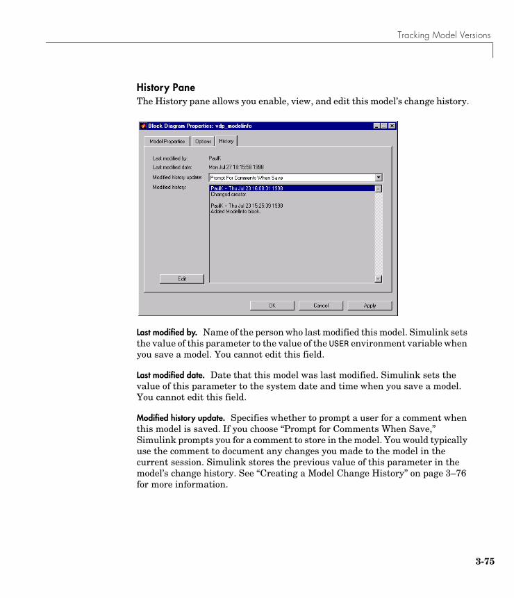
Tracking Model Versions
3-75
History PaneThe History pane allows you enable, view, and edit this model’s change history.
Last modified by. Name of the person who last modified this model. Simulink setsthe value of this parameter to the value of the USER environment variable whenyou save a model. You cannot edit this field.
Last modified date. Date that this model was last modified. Simulink sets thevalue of this parameter to the system date and time when you save a model.You cannot edit this field.
Modified history update. Specifies whether to prompt a user for a comment whenthis model is saved. If you choose “Prompt for Comments When Save,”Simulink prompts you for a comment to store in the model. You would typicallyuse the comment to document any changes you made to the model in thecurrent session. Simulink stores the previous value of this parameter in themodel’s change history. See “Creating a Model Change History” on page 3–76for more information.

3 Creating a Model
3-76
Modified history. History of modifications of this model. Simulink compiles thehistory from comments entered by users when they update the model. You canedit the history at any time by selecting the adjacent Edit button.
Creating a Model Change HistorySimulink allows you to create and store a record of changes to a model in themodel itself. Simulink compiles the history automatically from comments thatyou or other users enter when they save changes to a model.
Logging ChangesTo start a change history, select the “Prompt for Comments When Save” optionfrom the History pane on the Simulink Model Properties dialog box. The nexttime you save the model, Simulink displays a Log Change dialog box.
If you want to add an item to the model’s change history, enter the item in theModified Comments edit field and click the Save button. If you do not want toenter an item for this session, uncheck the Include “Modified Contents” in“Modified History” option. If you want to discontinue change logging, uncheckthe Show this dialog box next time when save option.

Tracking Model Versions
3-77
Editing the Change HistoryTo edit the change history for a model, click the Edit button on the SimulinkModel Properties dialog box. Simulink displays the model’s history in aModification History dialog box.
Edit the history displayed in the dialog and select Apply or OK to save thechanges.
Version Control PropertiesSimulink stores version control information in a model as model parameters.You can access this information from the MATLAB command line or from anM-file, using the Simulink get_param command. The following table describesthe model parameters used by Simulink to store version control information.
Property Description
Created Date created
Creator Name of the person who created this model
ModifiedBy Person who last modified this model
ModifiedByFormat Format of the ModifiedBy parameter. Valuecan be an string. The string can include thetag %<Auto>. Simulink replaces the tag withthe current value of the USER environmentvariable.
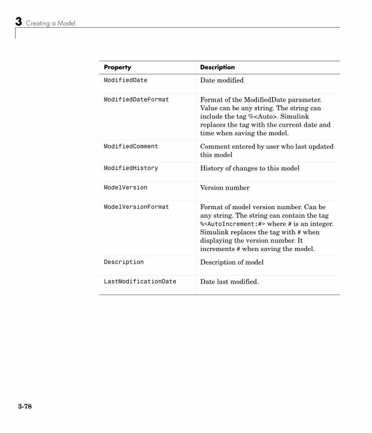
3 Creating a Model
3-78
ModifiedDate Date modified
ModifiedDateFormat Format of the ModifiedDate parameter.Value can be any string. The string caninclude the tag %<Auto>. Simulinkreplaces the tag with the current date andtime when saving the model.
ModifiedComment Comment entered by user who last updatedthis model
ModifiedHistory History of changes to this model
ModelVersion Version number
ModelVersionFormat Format of model version number. Can beany string. The string can contain the tag%<AutoIncrement:#> where # is an integer.Simulink replaces the tag with # whendisplaying the version number. Itincrements # when saving the model.
Description Description of model
LastModificationDate Date last modified.
Property Description
Ending a Simulink Session
3-79
Ending a Simulink SessionTerminate a Simulink session by closing all Simulink windows.
Terminate a MATLAB session by choosing one of these commands from theFile menu:
• On a Microsoft Windows system: Exit MATLAB
• On a UNIX system: Quit MATLAB

3 Creating a Model
3-80
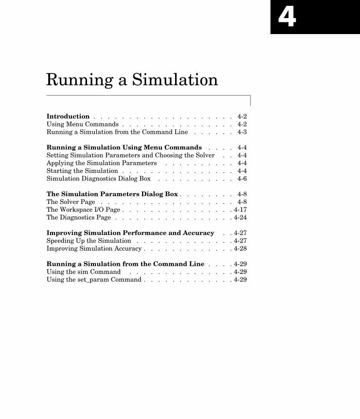
4
Running a Simulation
Introduction . . . . . . . . . . . . . . . . . . . . 4-2Using Menu Commands . . . . . . . . . . . . . . . . 4-2Running a Simulation from the Command Line . . . . . . 4-3
Running a Simulation Using Menu Commands . . . . 4-4Setting Simulation Parameters and Choosing the Solver . . 4-4Applying the Simulation Parameters . . . . . . . . . . 4-4Starting the Simulation . . . . . . . . . . . . . . . . 4-4Simulation Diagnostics Dialog Box . . . . . . . . . . . 4-6
The Simulation Parameters Dialog Box . . . . . . . . 4-8The Solver Page . . . . . . . . . . . . . . . . . . . 4-8The Workspace I/O Page . . . . . . . . . . . . . . . . 4-17The Diagnostics Page . . . . . . . . . . . . . . . . . 4-24
Improving Simulation Performance and Accuracy . . 4-27Speeding Up the Simulation . . . . . . . . . . . . . . 4-27Improving Simulation Accuracy . . . . . . . . . . . . . 4-28
Running a Simulation from the Command Line . . . . 4-29Using the sim Command . . . . . . . . . . . . . . . 4-29Using the set_param Command . . . . . . . . . . . . . 4-29
4 Running a Simulation
4-2
IntroductionYou can run a simulation either by using Simulink menu commands or byentering commands in the MATLAB command window.
Many users use menu commands while they develop and refine their models,then enter commands in the MATLAB command window to run the simulationin “batch” mode.
Using Menu CommandsRunning a simulation using menu commands is easy and interactive. Thesecommands let you select an ordinary differential equation (ODE) solver anddefine simulation parameters without having to remember command syntax.An important advantage is that you can perform certain operationsinteractively while a simulation is running:
• You can modify many simulation parameters, including the stop time, thesolver, and the maximum step size.
• You can change the solver.
• You can simulate another system at the same time.
• You can click on a line to see the signal carried on that line on a floating(unconnected) Scope or Display block.
• You can modify the parameters of a block, as long as you do not cause achange in:
- The number of states, inputs, or outputs
- The sample time
- The number of zero crossings
- The vector length of any block parameters
- The length of the internal block work vectors
You cannot make changes to the structure of the model, such as adding ordeleting lines or blocks, during a simulation. If you need to make these kindsof changes, you need to stop the simulation, make the change, then start thesimulation again to see the results of the change.

Introduction
4-3
Running a Simulation from the Command LineRunning a simulation from the command line has these advantages overrunning a simulation using menu commands:
• You can simulate M-file and MEX-file models, as well as Simulink blockdiagram models.
• You can run a simulation from an M-file, allowing simulation and blockparameters to be changed iteratively.
For more information, see “Running a Simulation from the Command Line” onpage 4-29.
4 Running a Simulation
4-4
Running a Simulation Using Menu CommandsThis section discusses how to use Simulink menu commands and theSimulation Parameters dialog box to run a simulation.
Setting Simulation Parameters and Choosing the SolverYou set the simulation parameters and select the solver by choosingParameters from the Simulation menu. Simulink displays the SimulationParameters dialog box, which uses three “pages” to manage simulationparameters:
• The Solver page allows you to set the start and stop times, choose the solverand specify solver parameters, and choose some output options.
• The Workspace I/O page manages input from and output to the MATLABworkspace.
• The Diagnostics page allows you to select the level of warning messagesdisplayed during a simulation.
Each page of the dialog box, including the parameters you set on the page, isdiscussed in detail in “The Simulation Parameters Dialog Box” on page 4-8.
You can specify parameters as valid MATLAB expressions, consisting ofconstants, workspace variable names, MATLAB functions, and mathematicaloperators.
Applying the Simulation ParametersAfter you have set the simulation parameters and selected the solver, you areready to apply them to your model. Press the Apply button on the bottom of thedialog box to apply the parameters to the model. To apply the parameters andclose the dialog box, press the Close button.
Starting the SimulationAfter you have applied the solver and simulation parameters to your model,you are ready to run the simulation. Select Start from the Simulation menu torun the simulation. You can also use the keyboard shortcut, Ctrl-T. When youselect Start, the menu item changes to Stop.

Running a Simulation Using Menu Commands
4-5
Your computer beeps to signal the completion of the simulation.
Note A common mistake that new Simulink users make is to start asimulation while the Simulink block library is the active window. Make sureyour model window is the active window before starting a simulation.
To stop a simulation, choose Stop from the Simulation menu. The keyboardshortcut for stopping a simulation is Ctrl-T, the same as for starting asimulation.
You can suspend a running simulation by choosing Pause from the Simulationmenu. When you select Pause, the menu item changes to Continue. Youproceed with a suspended simulation by choosing Continue.
If the model includes any blocks that write output to a file or to the workspace,or if you select output options on the Simulation Parameters dialog box,Simulink writes the data when the simulation is terminated or suspended.
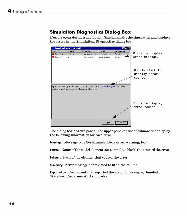
4 Running a Simulation
4-6
Simulation Diagnostics Dialog BoxIf errors occur during a simulation, Simulink halts the simulation and displaysthe errors in the Simulation Diagnostics dialog box.
The dialog box has two panes. The upper pane consist of columns that displaythe following information for each error.
Message. Message type (for example, block error, warning, log)
Source. Name of the model element (for example, a block) that caused the error.
Fullpath. Path of the element that caused the error.
Summary. Error message abbreviated to fit in the column.
Reported by. Component that reported the error (for example, Simulink,Stateflow, Real-Time Workshop, etc).
Double-click to display error source.
Click to display error source.
Click to display error message.
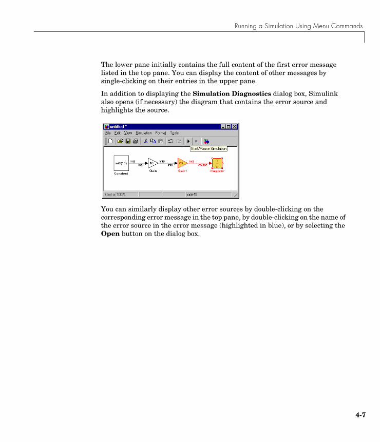
Running a Simulation Using Menu Commands
4-7
The lower pane initially contains the full content of the first error messagelisted in the top pane. You can display the content of other messages bysingle-clicking on their entries in the upper pane.
In addition to displaying the Simulation Diagnostics dialog box, Simulinkalso opens (if necessary) the diagram that contains the error source andhighlights the source.
You can similarly display other error sources by double-clicking on thecorresponding error message in the top pane, by double-clicking on the name ofthe error source in the error message (highlighted in blue), or by selecting theOpen button on the dialog box.

4 Running a Simulation
4-8
The Simulation Parameters Dialog BoxThis section discusses the simulation parameters, which you specify either onthe Simulation Parameters dialog box or using the sim (see sim on page 4-30)and simset (see simset on page 4-32) commands. Parameters are described asthey appear on the dialog box pages.
This table summarizes the actions performed by the dialog box buttons, whichappear on the bottom of each dialog box page.
The Solver PageThe Solver page appears when you first choose Parameters from theSimulation menu or when you select the Solver tab.
The Solver page allows you to:
• Set the simulation start and stop times
• Choose the solver and specify its parameters
• Select output options
Table 4-1: Simulation Parameters Dialog Box Buttons
Button Action
Ok Applies the parameter values and closes the dialog box. Duringa simulation, the parameter values are applied immediately.
Cancel Changes the parameter values back to the values they hadwhen the dialog box was most recently opened and closes thedialog box.
Help Displays help text for the dialog box page.
Apply Applies the current parameter values and keeps the dialog boxopen. During a simulation, the parameter values are appliedimmediately.

The Simulation Parameters Dialog Box
4-9
Simulation TimeYou can change the start time and stop time for the simulation by entering newvalues in the Start time and Stop time fields. The default start time is 0.0seconds and the default stop time is 10.0 seconds.
Simulation time and actual clock time are not the same. For example, runninga simulation for 10 seconds will usually not take 10 seconds. The amount oftime it takes to run a simulation depends on many factors, including themodel’s complexity, the solver’s step sizes, and the computer’s clock speed.
SolversSimulation of Simulink models involves the numerical integration of sets ofordinary differential equations (ODEs). Simulink provides a number of solversfor the simulation of such equations. Because of the diversity of dynamicsystem behavior, some solvers may be more efficient than others at solving aparticular problem. To obtain accurate and fast results, take care whenchoosing the solver and setting parameters.
You can choose between variable-step and fixed-step solvers. Variable-stepsolvers can modify their step sizes during the simulation. They provide errorcontrol and zero crossing detection. Fixed-step solvers take the same step size

4 Running a Simulation
4-10
during the simulation. They provide no error control and do not locate zerocrossings. For a thorough discussion of solvers, see Using MATLAB.
Default solvers. If you do not choose a solver, Simulink chooses one based onwhether your model has states:
• If the model has continuous states, ode45 is used. ode45 is an excellentgeneral purpose solver. However, if you know that your system is stiff and ifode45 is not providing acceptable results, try ode15s. For a definition of stiff,see the note at the end of the section “Variable-step solvers” on page 4-11.
• If the model has no continuous states, Simulink uses the variable-step solvercalled discrete and displays a message indicating that it is not using ode45.Simulink also provides a fixed-step solver called discrete. This model showsthe difference between the two discrete solvers.
With sample times of 0.5 and 0.75, the fundamental sample time for themodel is 0.25 seconds. The difference between the variable-step and thefixed-step discrete solvers is the time vector that each generates.
The fixed-step discrete solver generates this time vector:[0.0 0.25 0.5 0.75 1.0 1.25 ...]
The variable-step discrete solver generates this time vector:[0.0 0.5 0.75 1.0 1.5 2.0 2.25 ...]
The step size of the fixed-step discrete solver is the fundamental sampletime. The variable-step discrete solver takes the largest possible steps.

The Simulation Parameters Dialog Box
4-11
Variable-step solvers. You can choose these variable-step solvers: ode45, ode23,ode113, ode15s, ode23s, and discrete. The default is ode45 for systems withstates, or discrete for systems with no states:
• ode45 is based on an explicit Runge-Kutta (4,5) formula, theDormand-Prince pair. It is a one-step solver; that is, in computing y(tn), itneeds only the solution at the immediately preceding time point, y(tn–1). Ingeneral, ode45 is the best solver to apply as a “first try” for most problems.
• ode23 is also based on an explicit Runge-Kutta (2,3) pair of Bogacki andShampine. It may be more efficient than ode45 at crude tolerances and in thepresence of mild stiffness. ode23 is a one-step solver.
• ode113 is a variable order Adams-Bashforth-Moulton PECE solver. It may bemore efficient than ode45 at stringent tolerances. ode113 is a multistepsolver; that is, it normally needs the solutions at several preceding timepoints to compute the current solution.
• ode15s is a variable order solver based on the numerical differentiationformulas (NDFs). These are related to but are more efficient than thebackward differentiation formulas, BDFs (also known as Gear’s method).Like ode113, ode15s is a multistep method solver. If you suspect that aproblem is stiff or if ode45 failed or was very inefficient, try ode15s.
• ode23s is based on a modified Rosenbrock formula of order 2. Because it is aone-step solver, it may be more efficient than ode15s at crude tolerances. Itcan solve some kinds of stiff problems for which ode15s is not effective.
• ode23t is an implementation of the trapezoidal rule using a “free”interpolant. Use this solver if the problem is only moderately stiff and youneed a solution without numerical damping.
• ode23tb is an implementation of TR-BDF2, an implicit Runge-Kutta formulawith a first stage that is a trapezoidal rule step and a second stage that is abackward differentiation formula of order two. By construction, the sameiteration matrix is used in evaluating both stages. Like ode23s, this solvermay be more efficient than ode15s at crude tolerances.
• discrete (variable-step) is the solver Simulink chooses when it detects thatyour model has no continuous states.

4 Running a Simulation
4-12
Note For a stiff problem, solutions can change on a time scale that is veryshort compared to the interval of integration, but the solution of interestchanges on a much longer time scale. Methods not designed for stiff problemsare ineffective on intervals where the solution changes slowly because theyuse time steps small enough to resolve the fastest possible change. Jacobianmatrices are generated numerically for ode15s and ode23s. For moreinformation, see Shampine, L. F., Numerical Solution of Ordinary DifferentialEquations, Chapman & Hall, 1994.
Fixed-step solvers. You can choose these fixed-step solvers: ode5, ode4, ode3,ode2, ode1, and discrete:
• ode5 is the fixed-step version of ode45, the Dormand-Prince formula.
• ode4 is RK4, the fourth-order Runge-Kutta formula.
• ode3 is the fixed-step version of ode23, the Bogacki-Shampine formula.
• ode2 is Heun’s method, also known as the improved Euler formula.
• ode1 is Euler’s method.
• discrete (fixed-step) is a fixed-step solver that performs no integration. It issuitable for models having no states and for which zero crossing detectionand error control are not important.
If you think your simulation may be providing unsatisfactory results, see“Improving Simulation Performance and Accuracy” on page 4-27.
Solver OptionsThe default solver parameters provide accurate and efficient results for mostproblems. In some cases, however, tuning the parameters can improveperformance. (For more information about tuning these parameters, see“Improving Simulation Performance and Accuracy” on page 4-27). You cantune the selected solver by changing parameter values on the Solver panel.
Step SizesFor variable-step solvers, you can set the maximum and suggested initial stepsize parameters. By default, these parameters are automatically determined,indicated by the value auto.
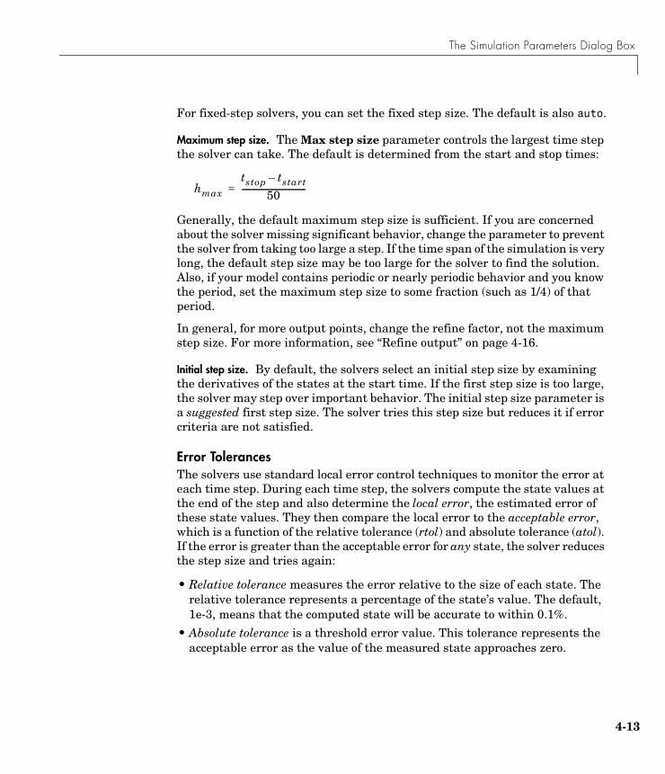
The Simulation Parameters Dialog Box
4-13
For fixed-step solvers, you can set the fixed step size. The default is also auto.
Maximum step size. The Max step size parameter controls the largest time stepthe solver can take. The default is determined from the start and stop times:
Generally, the default maximum step size is sufficient. If you are concernedabout the solver missing significant behavior, change the parameter to preventthe solver from taking too large a step. If the time span of the simulation is verylong, the default step size may be too large for the solver to find the solution.Also, if your model contains periodic or nearly periodic behavior and you knowthe period, set the maximum step size to some fraction (such as 1/4) of thatperiod.
In general, for more output points, change the refine factor, not the maximumstep size. For more information, see “Refine output” on page 4-16.
Initial step size. By default, the solvers select an initial step size by examiningthe derivatives of the states at the start time. If the first step size is too large,the solver may step over important behavior. The initial step size parameter isa suggested first step size. The solver tries this step size but reduces it if errorcriteria are not satisfied.
Error TolerancesThe solvers use standard local error control techniques to monitor the error ateach time step. During each time step, the solvers compute the state values atthe end of the step and also determine the local error, the estimated error ofthese state values. They then compare the local error to the acceptable error,which is a function of the relative tolerance (rtol) and absolute tolerance (atol).If the error is greater than the acceptable error for any state, the solver reducesthe step size and tries again:
• Relative tolerance measures the error relative to the size of each state. Therelative tolerance represents a percentage of the state’s value. The default,1e-3, means that the computed state will be accurate to within 0.1%.
• Absolute tolerance is a threshold error value. This tolerance represents theacceptable error as the value of the measured state approaches zero.
hmax
tstop tstart–
50--------------------------------=

4 Running a Simulation
4-14
The error for the ith state, ei, is required to satisfy.
The figure below shows a plot of a state and the regions in which the acceptableerror is determined by the relative tolerance and the absolute tolerance:
If you specify auto (the default), Simulink sets the absolute tolerance for eachstate initially to 1e-6. As the simulation progresses, Simulink resets theabsolute tolerance for each state to the maximum value that the state hasassumed thus far times the relative tolerance for that state. Thus, if a stategoes from 0 to 1 and reltol is 1e-3, then by the end of the simulation theabstol is set to 1e-3 also. If a state goes from 0 to 1000, then the abstol is setto 1.
If the computed setting is not suitable, you can determine an appropriatesetting yourself. You might have to run a simulation more than once todetermine an appropriate value for the absolute tolerance. If the magnitudesof the states vary widely, it might be appropriate to specify different absolutetolerance values for different states. You can do this on the Integrator block’sdialog box.
The Maximum Order for ode15sThe ode15s solver is based on NDF formulas of order one through five.Although the higher order formulas are more accurate, they are less stable. Ifyour model is stiff and requires more stability, reduce the maximum order to 2(the highest order for which the NDF formula is A-stable). When you choose theode15s solver, the dialog box displays this parameter.
As an alternative, you might try using the ode23s solver, which is a fixed-step,lower order (and A-stable) solver.
ei max rtol xi atoli,×( )≤
atol
rtol*|x|Region in which rtol determines acceptable error
Region in which atol determines acceptable errorSta
te
Time
The Simulation Parameters Dialog Box
4-15
Multitasking OptionsIf you select a fixed-step solver, the Solver page of the Simulation Parametersdialog box displays a Mode options list. The list allows you to select one of thefollowing simulation modes.
MultiTasking. This mode issues an error if it detects an illegal sample ratetransition between blocks, that is, a direct connection between blocks operatingat different sample rates. In real-time multitasking systems, illegal samplerate transitions between tasks can result in a task’s output not being availablewhen needed by another task. By checking for such transitions, multitaskingmode helps you to create valid models of real-world multitasking systems,where sections of your model represent concurrent tasks.
Use rate transition blocks to eliminate illegal rate transitions from your model.Simulink provides two such blocks: Unit Delay (see Unit Delay on page 8-214)and Zero-Order Hold (see Zero-Order Hold on page 8-221). To eliminate anillegal slow-to-fast transition, insert a Unit Delay block running at the slowrate between the slow output port and the fast input port. To eliminate anillegal fast-to-slow transition, insert a Zero-Order Hold block running at theslow rate between the fast output port and the slow input port. For moreinformation, see Chapter 7, “Models with Multiple Sample Rates,” in theReal-Time Workshop Users Guide.
SingleTasking. This mode does not check for sample rate transitions amongblocks. This mode is useful when you are modeling a single-tasking system. Insuch systems, task synchronization is not an issue.
Auto. This option causes Simulink to use single-tasking mode if all blocksoperate at the same rate and multitasking mode if the model contains blocksoperating at different rates.
Output OptionsThe Output options area of the dialog box enables you to control how muchoutput the simulation generates. You can choose from three popup options:
• Refine output
• Produce additional output
• Produce specified output only

4 Running a Simulation
4-16
Refine output. The Refine output choice provides additional output points whenthe simulation output is too coarse. This parameter provides an integernumber of output points between time steps; for example, a refine factor of 2provides output midway between the time steps, as well as at the steps. Thedefault refine factor is 1.
To get smoother output, it is much faster to change the refine factor instead ofreducing the step size. When the refine factor is changed, the solvers generateadditional points by evaluating a continuous extension formula at those points.Changing the refine factor does not change the steps used by the solver.
The refine factor applies to variable-step solvers and is most useful when usingode45. The ode45 solver is capable of taking large steps; when graphingsimulation output, you may find that output from this solver is not sufficientlysmooth. If this is the case, run the simulation again with a larger refine factor.A value of 4 should provide much smoother results.
Produce additional output. The Produce additional output choice enables you tospecify directly those additional times at which the solver generates output.When you select this option, Simulink displays an Ouput Times field on theSolver page. Enter a MATLAB expression in this field that evaluates to anadditional time or a vector of additional times. The additional output isproduced using a continuous extension formula at the additional times. Unlikethe refine factor, this option changes the simulation step size so that time stepscoincide with the times that you have specified for additional output.
Produce specified output only. The Produce specified output only choice providessimulation output only at the specified output times. This option changes thesimulation step size so that time steps coincide with the times that you havespecified for producing output. This choice is useful when comparing differentsimulations to ensure that the simulations produce output at the same times.
Comparing Output options. A sample simulation generates output at these times:
0, 2.5, 5, 8.5, 10
Choosing Refine output and specifying a refine factor of 2 generates output atthese times:
0, 1.25, 2.5, 3.75, 5, 6.75, 8.5, 9.25, 10
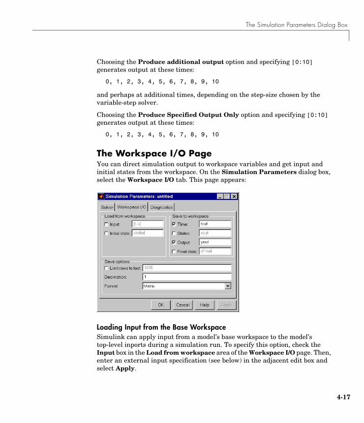
The Simulation Parameters Dialog Box
4-17
Choosing the Produce additional output option and specifying [0:10]generates output at these times:
0, 1, 2, 3, 4, 5, 6, 7, 8, 9, 10
and perhaps at additional times, depending on the step-size chosen by thevariable-step solver.
Choosing the Produce Specified Output Only option and specifying [0:10]generates output at these times:
0, 1, 2, 3, 4, 5, 6, 7, 8, 9, 10
The Workspace I/O PageYou can direct simulation output to workspace variables and get input andinitial states from the workspace. On the Simulation Parameters dialog box,select the Workspace I/O tab. This page appears:
Loading Input from the Base WorkspaceSimulink can apply input from a model’s base workspace to the model’stop-level inports during a simulation run. To specify this option, check theInput box in the Load from workspace area of the Workspace I/O page. Then,enter an external input specification (see below) in the adjacent edit box andselect Apply.