Starch GelatinizationMath 512, Milestone 5

Greg Hayes, Brandon Farmer, Brian Bourdon

December 8th, 2004

1 Introduction

Starch is a long chain of sugar molecules called a polysaccharide [1]. Starches differ by thepercentage amounts of amylose and amylopectin, the sugars that form the starch [2]. Duringheating of a starch, these sugars break down, or lose order, which allows for water absorptionand therefore swelling of the granule [2]. This process, called gelatinization occurs between58◦C and 75◦C [7].

Our investigations will be focusing on mathematically modeling the gelatinization frontof potatoes and rice. Our first goal is to know when and what parts of starches havegelatinized during the heating (cooking) process. By increasing the level of understandingof the gelatinization process it is possible to optimize industrial production of these types offoods while controlling quality and stability [6]. This in turn will lead to a more efficientlyproduced final product with improved taste and texture [5].

Previous research in this area has been extensive and results have varied. Chi Kai showsa linear relationship between time and water uptake during the gelatinization process [4].Sharpe [3], Landman, and McGuinness [5] show a nonlinear relationship in their results. Ourpreliminary results and heat transfer model suggest a nonlinear relationship. Ogawa et al.show that water penetrates into rice unequally during heating [8]. This indicates a possibilitythat gelatinization does not move with a uniform front. Our early experiments show thatthis front, in potatoes, is somewhat uniform, and our model is based on the assumptionthat the front is uniform. More experimentation and modeling is necessary to determine theactual shape of the front.

2 Mathematical Model

2.1 Introduction

A number of factors must be considered in order to model the gelatinization in a potatoduring the heating (cooking) process. Based on our literature review and experimentationwe have developed several assumptions that will allow us to mathematically describe the lossof order during the cooking process. These assumptions will more easily allow us to derive a

1

mathematical representation of the gelatinization process without drastically changing thesolutions. Assumptions:

• The potato is spherical. We will form the potatoes into spheres before experimentation.This is necessary for us to mathematically model the gelatinizaton front.

• The level of gelatinization can be determined by measuring or modeling the temper-ature inside the potato. This allows us to solve the heat equation on a sphere andmodel the isotherm as it moves through the potato to measure the loss of order.

• The potato is homogeneous throughout. This will be accomplished by skinning thepotato before experimentation. This allows for an easier calculation of the heat fluxinto the potato.

• The gelatinization moves on a uniform front. In other words, the geometry of thegelatinization front evolves axis-symmetrically. Some of the literature states that thisis not true for starches, but our experiments have shown that this assumption holds.

• Little swelling occurs during the gelatinization process and we therefore consider theradius constant during cooking. Our experimentation shows this and we have hypoth-esized that it may be due to the fact that the water present in the raw potato helpsstimulate the gelatinization of the cells.

• Based on initial experimentation, we notice that the boundary between gelatinized toungelatinized starch is relatively small in consideration to the size of the potato. Pleasesee Figure 1.

2.2 Theoretical

Based on our assumption that gelatinization can be determined by the temperature of thepotato (63◦C indicates full gelatinization), we can model the isotherm inside the potato asthe gelatinization front. This isotherm is determined by solving the heat equation. Thegeneral heat equation is

∂U

∂t= α2∇2U. (1)

Assuming that our potatoes are spherical allows us to use the heat equation on a sphere asour model. Using the variable transformations:

x = r sin(φ) cos(θ), (2)

y = r sin(φ) sin(θ), (3)

z = r cos(φ). (4)

we obtain the heat equation in spherical coordinates:

Ut =1

r2α2

(2rUr + r2Urr +

cos(φ)

sin(φ)Uφ + Uφφ +

1

sin2(φ)Uθθ

). (5)

2

Next, by applying our initial assumption that this phenomena is axis-symmetric (independentof (θ) and (φ)), we have

∂U

∂φ=

∂U

∂θ= 0. (6)

We can now simplify (5) to

Ut = α2

(2Ur

r+ Urr

). (7)

2.3 Boundary Conditions

Based on the temperature of our bath and the assumption that the outer layer of the potatois instantly the temperature of the bath once submerged, we have the boundary condition

U(c, t) = 75◦C. (8)

After taking the temperature readings of the center of a potato during experimentation,we found the center to be at room temperature (approximately 21.2◦C). This gives us thefollowing boundary condition:

U(0, 0) = 21.2◦C. (9)

2.4 Non-Dimensional Model

Making our variables dimensionless gives us the following:

t =

(tc2

α2

), (10)

r =(r

c

), (11)

U =

(U − Uinitial

Ufinal − Uinitial

), (12)

(13)

When we apply our dimensionless variables to (7) , we have our dimensionless heat equationon a sphere:

Ut =2Ur

r+ Urr. (14)

With boundary conditions:

U(0, 0) = 0 (15)

U(1, t) = 1 (16)

3

2.5 Solving the Equation

We will use the separation of variables technique to solve (14). To do this we assume U isin the form (Note: from here on we assume all variables are dimensionless for simplicity)

U(r, t) = R(r)T (t). (17)

By taking partial derivatives, we have

Ut = RT ′, (18)

Ur = R′T, (19)

Urr = R′′T. (20)

We plug (18), (19), and (20) into (17), thus:

RT ′ =(

2

r

)R′′T + R′T. (21)

Dividing by U givesT ′

T=

(2

r

)R′′

R+

R′

R. (22)

Let the eigenvalues be k, where k is nonnegative. We therefore define our constant equal to−k2. If our constant were positive it would yield solutions that are exponential, which is notdesirable in our case. Therefore,

T ′

T= −k2, (23)

(2

r

)R′′

R+

R′

R= −k2, (24)

or,

T ′ + k2T = 0, (25)

R′′ +2

rR′ + k2R = 0. (26)

Notice that (25) is an ODE yielding solutions in the form

T (t) = e(−k2t). (27)

Equation (26) is not quite a Bessel equation of order zero because of the k2. We can absorbk2 by a change of variable. If we scale r as t = λr, where λ is to be determined. Thenddr

=(

ddt

) (dtdr

)λ d2

dt2and (26) becomes, after division by λ,

tR′′ + R′ +k2

λ2tR = 0. (28)

Thus, k2 can be absorbed by choosing λ = k. Notice (28) then becomes a Bessel equationof order zero with general solution R(t) = AJ0(t) + BY0(t). Therefore, we have

R(t) = AJ0(t) + BY0(t) = AJ0(kr) + BY0(kr), (29)

4

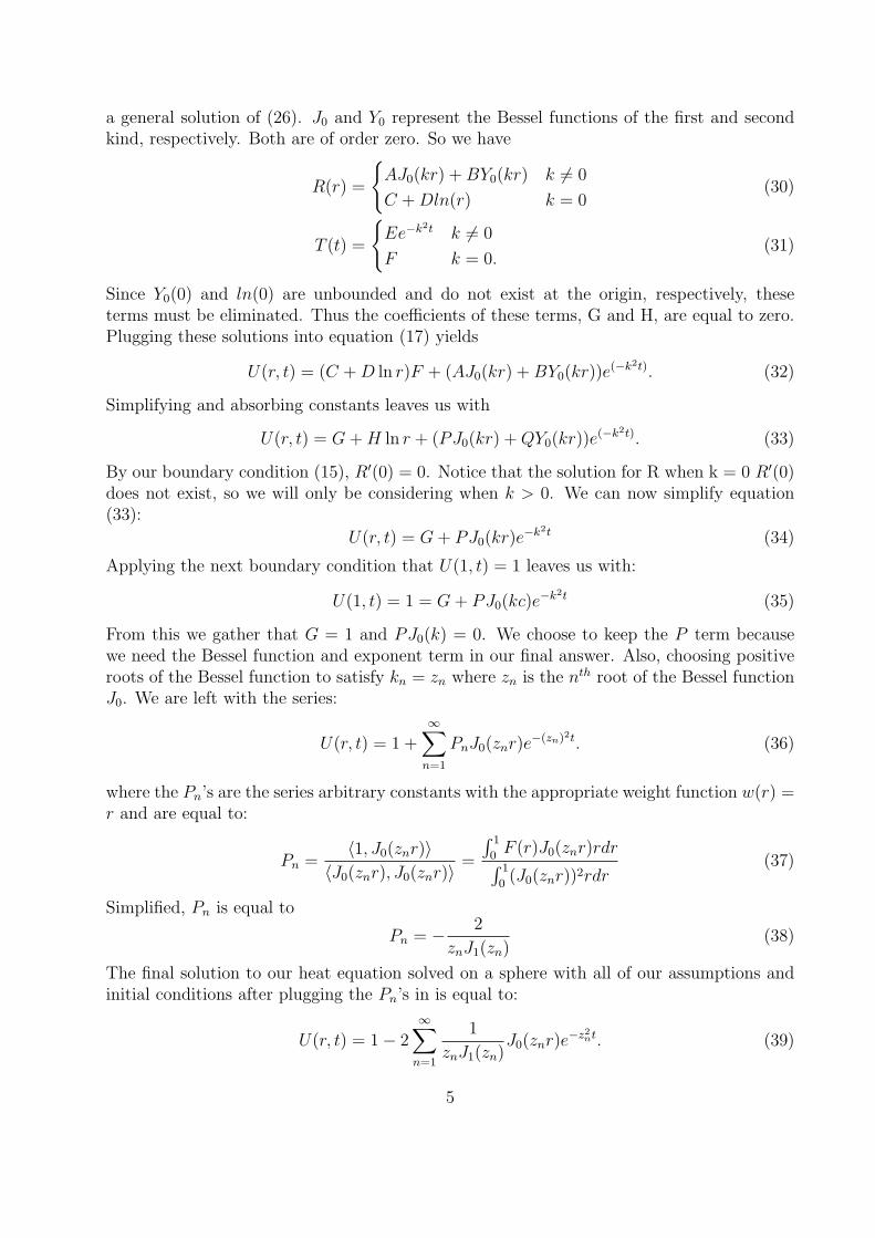
a general solution of (26). J0 and Y0 represent the Bessel functions of the first and secondkind, respectively. Both are of order zero. So we have

R(r) =

{AJ0(kr) + BY0(kr) k 6= 0

C + Dln(r) k = 0(30)

T (t) =

{Ee−k2t k 6= 0

F k = 0.(31)

Since Y0(0) and ln(0) are unbounded and do not exist at the origin, respectively, theseterms must be eliminated. Thus the coefficients of these terms, G and H, are equal to zero.Plugging these solutions into equation (17) yields

U(r, t) = (C + D ln r)F + (AJ0(kr) + BY0(kr))e(−k2t). (32)

Simplifying and absorbing constants leaves us with

U(r, t) = G + H ln r + (PJ0(kr) + QY0(kr))e(−k2t). (33)

By our boundary condition (15), R′(0) = 0. Notice that the solution for R when k = 0 R′(0)does not exist, so we will only be considering when k > 0. We can now simplify equation(33):

U(r, t) = G + PJ0(kr)e−k2t (34)

Applying the next boundary condition that U(1, t) = 1 leaves us with:

U(1, t) = 1 = G + PJ0(kc)e−k2t (35)

From this we gather that G = 1 and PJ0(k) = 0. We choose to keep the P term becausewe need the Bessel function and exponent term in our final answer. Also, choosing positiveroots of the Bessel function to satisfy kn = zn where zn is the nth root of the Bessel functionJ0. We are left with the series:

U(r, t) = 1 +∞∑

n=1

PnJ0(znr)e−(zn)2t. (36)

where the Pn’s are the series arbitrary constants with the appropriate weight function w(r) =r and are equal to:

Pn =〈1, J0(znr)〉

〈J0(znr), J0(znr)〉 =

∫ 1

0F (r)J0(znr)rdr∫ 1

0(J0(znr))2rdr

(37)

Simplified, Pn is equal to

Pn = − 2

znJ1(zn)(38)

The final solution to our heat equation solved on a sphere with all of our assumptions andinitial conditions after plugging the Pn’s in is equal to:

U(r, t) = 1− 2∞∑

n=1

1

znJ1(zn)J0(znr)e

−z2nt. (39)

5

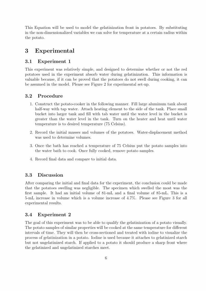
This Equation will be used to model the gelatinization front in potatoes. By substitutingin the non-dimensionalized variables we can solve for temperature at a certain radius withinthe potato.

3 Experimental

3.1 Experiment 1

This experiment was relatively simple, and designed to determine whether or not the redpotatoes used in the experiment absorb water during gelatinization. This information isvaluable because, if it can be proved that the potatoes do not swell during cooking, it canbe assumed in the model. Please see Figure 2 for experimental set-up.

3.2 Procedure

1. Construct the potato-cooker in the following manner. Fill large aluminum tank abouthalf-way with tap water. Attach heating element to the side of the tank. Place smallbucket into larger tank and fill with tab water until the water level in the bucket isgreater than the water level in the tank. Turn on the heater and heat until watertemperature is to desired temperature (75 Celsius).

2. Record the initial masses and volumes of the potatoes. Water-displacement methodwas used to determine volumes.

3. Once the bath has reached a temperature of 75 Celsius put the potato samples intothe water bath to cook. Once fully cooked, remove potato samples.

4. Record final data and compare to initial data.

3.3 Discussion

After comparing the initial and final data for the experiment, the conclusion could be madethat the potatoes swelling was negligible. The specimen which swelled the most was thefirst sample. It had an initial volume of 81-mL and a final volume of 85-mL. This is a5-mL increase in volume which is a volume increase of 4.7%. Please see Figure 3 for allexperimental results.

3.4 Experiment 2

The goal of this experiment was to be able to qualify the gelatinization of a potato visually.The potato samples of similar properties will be cooked at the same temperature for differentintervals of time. They will then be cross-sectioned and treated with iodine to visualize theprocess of gelatinization in a potato. Iodine is used because it attaches to gelatinized starchbut not ungelatinized starch. If applied to a potato it should produce a sharp front wherethe gelatinized and ungelatinized starches meet.

6

3.5 Procedure

1. Construct the potato-cooker in the following manner. Fill large aluminum tank abouthalf-way with tap water. Attach heating element to the side of the tank. Place smallbucket into larger tank and fill with tab water until the water level in the bucket isgreater than the water level in the tank. Turn on the heater and heat until watertemperature is to desired temperature (75 Celsius).

2. Carve potatoes into spheres of the same radius.

3. Once the water in the bucket has heated to the desired temperature, place the potatospheres into the bucket. Remove the potatoes at the desired interval (10 minutes).

4. Slice the potato spheres through the circumference.

5. Put on latex gloves and wet end of finger with iodine. Rub the iodine onto the potatocross-sections. Wait a couple of minutes and rinse the potato with water.

6. Take pictures of the potato cross-sections for analyzation.

3.6 Discussion

As seen in figure 7, the gelatinization front can be viewed as the barrier between the part ofthe potato stained purple (gelatinized) with iodine and the part of the potato which remainsungelatinized. As time progressed the gelatinization front moved closer to the center of thepotato. Matlab was used to analyze the pictures of the potato cross-sections and determinethe degree of gelatinization. This data will be used to check our model once the α value forour red potatoes is established in the next experiment.

3.7 Experiment 3

In this experiment the α value will be determined by takeing the temperature at the centerof a potato sphere with respect to time as the potato cooks. If this data is then graphed andlinearized, the result is a constant α. α is used in our model as the coefficient of thermaldiffusivity. A graph of just the experimental data before it was compared to the theoreticaldata for α determination can be found in figure 4.

3.8 Procedure

1. Set up the apparatus as in the two previous experiments.

2. Carve the potatoes into spheres of equal radii.

3. Drill a hole to the center of a potato sphere. Push isotherm into the center of thepotato. Seal the hole with petroleum jelly.

4. Connect the isotherm to the thermometer.

7

5. Repeat 3 for every potato used.

6. Once the water has reached the desired temperature, place the potatoes into the bucket.

7. Record temperature at the center of the potato every on minute.

8. Cook potatoes in water until the isotherm reads above the temperature of gelatinizationof the potatoes.

9. Remove the potatoes from the water.

10. Repeat if necessary.

3.9 Discussion

After the data was analyzed, a good alpha value was determined for our model. This alphavalue was then plugged into the mathematical model and the output was close to the datataken from the experiment.

4 Analysis and Results

Using Maple, a study of the behavior or our equation was completed. Non-dimensional plotsof both Temperature vs. Time and isotherms of our 63 degree gelatinization front wereconstructed. Please see figures 5 and 6 for the theoretical simulation of the temperature atthe center and the gelatinization isotherm, respectively. Using maple it is possible to enterthe initial water, potato, and gelatinization temperature, along with radius, α, and time thatthe potato is cooking. Please see appendix for a detailed Maple code. We can clearly see themovement of the gelatinization front thought the potato as time increases in the IsothermFigure. After analyzing the gelatinization front in the cut potatoes. It is easy to tell thatthe front moves in a more or less uniform fashion towards the center of the potato. In figure7, the dark areas are the gelatinized regions, while the lighter areas are the ungelatinizedregions. Using a matlab pixel counter, we were able to directly determine the ratio of blackto white pixels, and from there determine the percentage of gelatinization in the potato. Thematlab code used can be found in figure 8. Since the value of thermal diffusivity for the redpotato varies greatly with temperature, and varies slightly with position within the potato,we felt that a good average value of α was needed. To determine this value, we first plottedthe non-dimensionalized experimental data. Next, we ran a maple code to export data thatcorresponded to the experimental data that we had previously plotted. By adjusting thethermal diffusivity we were able to, in essence, achieve a best fit curve for our experimentaldata. The value of α that gave us this best fit curve has been said to be our ”average”thermal diffusivity and is equal to 0.027cm2/s. The plot showing how our experimental andtheoretical values compare for the center of the potato during cooking can be seen in figure9. Using this thermal diffusivity value, we were able to go back to our derived equation.By knowing the gelatinization temperature, the thermal diffusivity, and the time cooked,we were able to back out the value for the radius of gelatinization. Using this radius wecompared the circular area of the gelatinized to ungelatinized portion of the potato. These

8

values for the percentage of gelatinization in the potato were then compared to the actualpercentage of gelatinization that was found through the matlab program. A graph showinghow our expected gelatinization curve fits our experimentally observed gelatinization curvecan be seen in figure 10.

5 Conclusion

It is clear that, as the mathematical model depicted, the gelatinization front moved throughthe potato in a more or less uniform manor. We can say that this model represented thephysical phenomena that is happening inside the potato well, however, more variables needto be taken into account in order to more accurately represent the phenomena of starchgelatinization inside a potato. The reason that our theoretical curves do not perfectly matchthe experimental curve is because of error in our mathematical model. By incorporatingwater absorption into our model, we believe this will increase the amount of gelatinizationper time, and therefore yield better accuracy of the model.

5.1 Theoretical and Experimental Strengths and Weaknesses

Some of the strengths and weaknesses to our mathematical model include the following:

5.2 Strengths

• A solid and reasonably accurate model was created for finding out the percent ofgelatinization inside a potato during cooking as a function of time.

• We were able to take into consideration during the problem, Uwater, Upotato, density,thermal conductivity, and specific heat.

• There is no free convection term, which, at high temperature, can greatly influence theconduction of heat into a submerged sphere. At high temperature, convection within afluid is increased. This increased convection leads to increased heat transfer within thesystem. As heat transfer due to convection is increased, a mathematical approximationfor this phenomena must be present.

5.3 Weaknesses

• The skin of the potato was removed, simplifying the heat transfer problem.

• There is no attempt to include water absorption into the mathematical model. Al-though from our experimental data, we can reasonably say that no water was absorbedduring cooking, new volumetric and mass measurements may lead this project into adirection where water absorption plays an important role.

Some of the strengths and weaknesses in our experimental model include the following:

9

5.4 Strengths

• A low amount of water circulation was achieved, reducing the effect of forced convectiondue to the water heater during cooking.

• A good visual guide for the amount of starch gelatinization was employed.

5.5 Weaknesses

• It is not clear that the temperature of the water inside of our holding tank was exactlythe same as the temperature of the water going through the heater.

• The iodine method for detecting starch gelatinization is not very precise, and a goodway of quantifying the iodine method results is needed.

• Only one experimental trial was run, therefore giving us no insight as to the errorinvolved in this process. More trials need to be undertaken to have an idea of reliability.

6 Future Work

For the upcoming people working on this project we wish to display a few points we feelwould be a good starting point to build on our project.

• Find a better way to use the iodine method results, and run more experimental trials.Both of these will reduce error and increase reliability of our methods.

• At low temperatures a gelatinization football occurs. A good understanding of thebasis for this football could lead to new insights into the gelatinization of starches.

• Meet with the food scientists and investigate incorporating lipids and emulsifiers intothe mathematical model.

• Relax some of the assumptions that simplify the model to produce a more accuratemodel. The first relaxed assumption should be the water absorption assumption.

7 Acknowledgments

• Professor Rossi

• Lauren Rossi

• Math 512 students

• Food Science students

10

References

[1] P. Barham. The science of cooking. 2001.

[2] J. Blanshard. Starch: Properties and potential. Critical Reports on Applied Chemistry,58:33, 1987.

[3] K. Sharpe. Gelatinized Starch Investigation. Gelatinized starch investigation. 2004.

[4] C. Kai. Private correspondence concerning rice growth over time. 2004.

[5] K. A. Landman and M. J. McGuinness. Mathematical modeling: Case studies fromindustry. page 97.

[6] M.H. Lim and D. S. Reid. Thermal analysis of potato during frozen french fries produc-tion. 2002.

[7] M. P. Penfield and A. M.Campbell. Experimental food science. 1990.

[8] G.A. Glenn Y Ogawa et al. Histological structures of cooked rice grain. Agricultural andFood Chemistry, page 7019.

8 Appendix A: Maple Code> restart:

> with(plots):

Warning, the name changecoords has been redefined <br>> alpha:=.034103; c:=2.25;t[water]:=(70-20)/(70-20); t[potato]:=(20-20)/(70-20);t[gelat]:=(60-20)/(70-20);

α := 0.034103c := 2.25twater := 1tpotato := 0tgelat := 4/5

> Ubar:=t[water]+2*(t[potato]-t[water])*sum(1/(BesselJZeros(0,n)*BesselJ(1,BesselJZeros(0,n)))*BesselJ(0,BesselJZeros(0,n)*rbar)*exp(-(BesselJZeros(0,n)^2*timebar)),n=1..infinity);

Ubar := 1− 2∑∞

n=1BesselJ (0,BesselJZeros(0,n)rbar)e−(BesselJZeros(0,n))2timebar

BesselJZeros(0,n)BesselJ (1,BesselJZeros(0,n))

> G:=0: <br>for i from 0 to 30 do<br>evalf(subs(rbar=0, timebar=G, Ubar)): <br>G:=G+1/30; <br>enddo;

0.0G := 1/300.0010732260G := 1/150.0444663900G := 1/100.1516448866G := 2/150.2773494276G := 1/60.3956104036G := 1/5

0.4985131394G := 7

30

0.5853284300G := 4

15

0.6576307858G := 3/100.7175129306G := 1/30.7669888310G := 11

30

0.8078237420G := 2/5

0.8415112266G := 13

30

0.8692966738G := 7

15

0.8922120766G := 1/20.9111102839G := 8

15

0.9266952643G := 17

30

0.9395477944

G := 3/50.9501469085G := 19

30

0.9588876821G := 2/30.9660959330G := 7

10

0.9720403573G := 11

15

0.9769425418G := 23

30

0.9809852228G := 4/50.9843190977G := 5/60.9870684418G := 13

15

0.9893357414G := 9

10

0.9912055137G := 14

15

0.9927474575G := 29

30

0.9940190511G := 10.9950676953G := 31

30

> plot(eval(Ubar,rbar=0), timebar=0..1,> labeldirections=[HORIZONTAL, VERTICAL], labels=["Non-Dimensional> Time","Non-Dimensional Temperature"], title= "Temperature vs Time> for Potato Center: r=0");

1

0.8

0.6

0.2

0

0.4

Non-Dimensional Time

10.80.60.20 0.4

Temperature vs Time for Potato Center: r=0

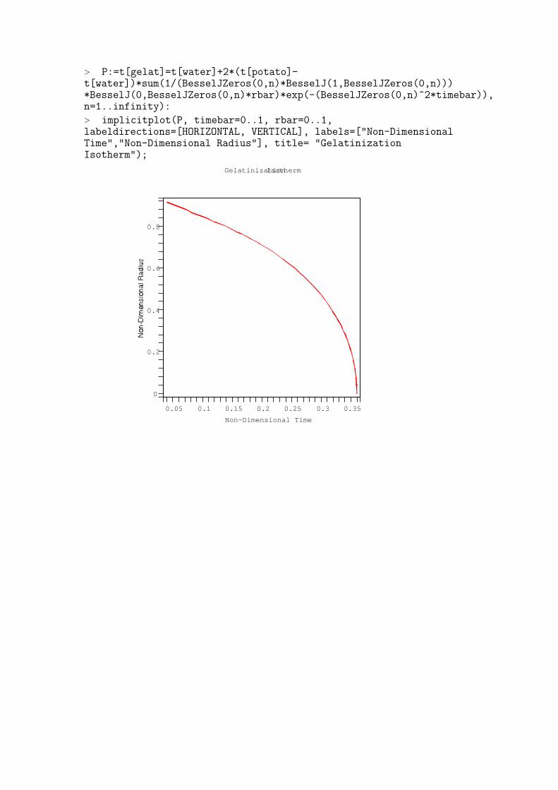
> P:=t[gelat]=t[water]+2*(t[potato]-t[water])*sum(1/(BesselJZeros(0,n)*BesselJ(1,BesselJZeros(0,n)))*BesselJ(0,BesselJZeros(0,n)*rbar)*exp(-(BesselJZeros(0,n)^2*timebar)),n=1..infinity):> implicitplot(P, timebar=0..1, rbar=0..1,labeldirections=[HORIZONTAL, VERTICAL], labels=["Non-DimensionalTime","Non-Dimensional Radius"], title= "GelatinizationIsotherm");

0.8

0.6

0.4

0.2

0

Non-Dimensional Time

0.350.30.250.20.10.05 0.15

Gelatinization Isotherm

Figure 1: Diagram representing Potato slice while it is being cooked.

Figure 2: Experimental Set-up Diagram

Figure 3: Experimental Data

0 5 10 15 20 25 30 35

20

30

40

50

60

70Actual Temperature vs Time plot at r=0

Tem

pera

ture

(o C)

Time (min)

Figure 4: Experimental Heat Increase in the Potato Center

1

0.8

0.6

0.2

0

0.4

Non-Dimensional Time

10.80.60.20 0.4

Temperature vs Time for Potato Center: r=0

Figure 5: Theoretical Temperature Change in Center of Potato with Time

0.8

0.6

0.4

0.2

0

Non-Dimensional Time

0.350.30.250.20.10.05 0.15

Gelatinization Isotherm

Figure 6: Theoretical Isotherm for 63 Degrees Celsius

Figure 7: Gelatinization in potato for various times

Figure 8: Matlab Code used in Determining the Percentage of Gelatinization

0 5 10 15 20 25 30 35

0.0

0.2

0.4

0.6

0.8

1.0

Time vs Temperature for Potato Center

Non

-Dim

ensi

onal

Tem

pera

ture

Time (Minutes)

Experimental Results Theoretical Approx., =.027 cm2/s

Figure 9: The above theoretical data was manipulated to find the best fit curve, giving usthe best fitting α value for our experiment.

10 15 20 25 30

0

20

40

60

80

100

Gelatinization vs Time

Perc

enta

ge G

elat

iniz

ed (%

)

Time (minutes)

Theoretical Approx. Experimental Value

Figure 10: Theoretical and Experimental Gelatinization Curves.