Star Formation Then and Now

Alyssa A. GoodmanHarvard-Smithsonian Center for Astrophysics

(currently on sabbatical at Yale)

cfa-www.harvard.edu/~agoodman

Star Formation Then and Now

“We should not hire a star formation theorist. Star formation is too messy a problem, and will never be solved. It’s not worthy of a theorist.”

—renowned astrophysicist at a top research university, 2002

The inspiration for this talk:

Star Formation Before Then

Global Instability (e.g. Jeans) Fragments Cloud

(hierarchically)

time~106 yearsHoyle 1953

Fragments Collapse UnderGravity into “Protostars”

time~105 years

Star Formation Before Then

A Group of Young“Zero-Age Main Sequence”

Stars is Born

Since “Then”

Does this look like a global

Jeans instability to

you?

All Between “Then” & “Now”Then≈1978 Now ≈2002

• Discovery of bipolar molecular outflows from young stars.• 1st all-sky surveys for embedded protostars (e.g. IRAS).• Discovery of line width-size relations, and attribution to

turbulence.• Understanding that most stars form in clusters and groups

(including binaries).• Debate over clump mass function, and relation to IMF.• First measurements of magnetic fields in molecular clouds.• Discovery of “giant” (>1 pc) Herbig-Haro flows.• 1st 3-D MHD simulations of molecular clouds.• First observations of protostellar disks (radio, IR, optical).• Discovery of extrasolar planets.

Outflows

MagnetohydrodynamicWaves

Thermal Motions

MHDTurbulence

InwardMotions

SNe/GRBH II Regions

Star Formation “Now”

Molecular or Dark Clouds

"Cores" and Outflows

An Heuristic View

Jets and Disks

Extrasolar System

1 p

c

What I’d like to talk about today

Molecular Spectral-Line Mapping Then & Now– Quick Tutorial

– Examples

1. The Value of MHD Simulations, The Spectral Correlation Function Goal is to improve simulations enough so that they

“match” observations empirically, then use the matching simulations to “experiment” with ISM conditions.

2. Outflows Then, Now, and Then, and Now… Episodicity, Energy Input, Moving Sources? How do

outflows effect clouds in the long run??

Beyond Now: The COMPLETE Survey

Radio Spectral-line Observations of Interstellar Clouds

Spectral Line Observations

BUT remember: Making this kind of map always loses 1 dimension.

Velocity as a "Fourth" DimensionSpectral Line Observations

Mountain RangeNo loss ofinformatio

n

Loss of1 dimension

Lee, Myers & Tafalla 2001.

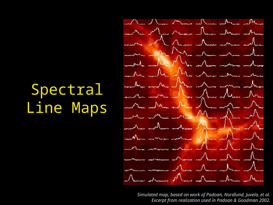
Spectral Line Maps

Simulated map, based on work of Padoan, Nordlund, Juvela, et al.Excerpt from realization used in Padoan & Goodman 2002.

Molecular Spectral Line Mapping:Then to Now

2000

2000

1990

1990

1980

1980

1970

1970

1960

1960

1950

1950

Year

100

101

102

103

104

Nch

an

nels, S

/N in

1 h

our, N

pix

els

102

103

104

105

106

107

108

(S/N

)*N

pix

els

*Nch

an

nels

Npixels

S/N

Product

Nchannels

That’s a one-thousand-fold“improvement” in 20 years.

Not What I Want to

Talk About

Courtesy BIMA Image Gallery

MHD Simulations as an Interpretive Tool

Stone, Gammie & Ostriker 1999•Driven Turbulence; M K; no gravity•Colors: log density•Computational volume: 2563

•Dark blue lines: B-field•Red : isosurface of passive contaminant after saturation

=0.01 =1

T / 10 K

nH 2 / 100 cm-3 B / 1.4 G 2

The Spectral Correlation Function (SCF)

Figure

fro

m F

alg

aro

ne e

t al. 1

99

4

Comparison SpectraComparison Spectra

Target Spectrum

Measures Similarity of Measures Similarity of Comparison Spectra to Comparison Spectra to

TargetTarget

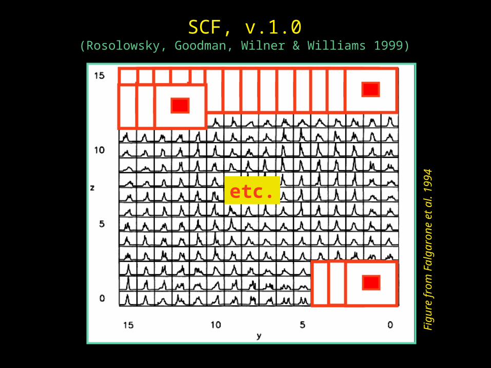
SCF, v.1.0(Rosolowsky, Goodman, Wilner & Williams 1999)

Figure

fro

m F

alg

aro

ne e

t al. 1

99

4

etc.

Application of the SCFgreyscale: TA=0.04 to 0. 3 K

Antenna Temperature Map

“Normalized” SCF Map

Data shown: C18O map of Rosette, courtesy M. Heyer et al.

Results: Padoan, Rosolowsky & Goodman 2001.

greyscale: while=low correlation; black=high

Ori

gin

al D

ata

Ra

ndo

miz

ed P

ositi

ons

SCF Distributions

Normalized C18O Data forRosette Molecular Cloud

Preliminary SCF (v.1.0) Comparisons1.0

0.8

0.6

0.4

0.2

0.01.21.00.80.60.40.20.0

Mean SCF Value

Cha

nge

in M

ean

SC

F w

ith R

ando

miz

atio

n Increasing Similarity of Spectra to Neighbors

G,O,SMHD +grav

Falgarone et alpure HD.

MacLow et al.MHD

L134A 12CO(2-1).

L1512 12CO(2-1)

Pol. 13CO(1-0)

L134A 13CO(1-0)

HCl2 C 18O Peaks

HCl2 C 18O

Rosette C 18O

Rosette C 18O Peaks

SNR

H I Survey

Rosette 13CO

Rosette 13CO Peaks

HLC

Increasing Similarity of A

LL

Spectra in M

ap

The Spectral Correlation Function as a Function of Spatial Scale

(v.2.0; Padoan et al. 2001)

Figure

fro

m F

alg

aro

ne e

t al. 1

99

4

v.2.0: Scale-Dependence of the SCF

Example for “Simulated Data” Padoan, Rosolowsky & Goodman 2001

ScaleS

pectral Correlation

Each plotted point is

“mean” of distribution

for that spatial lag.

How Well Do Numerical Models Match Reality,

Now?Pow

er-

Law

Slo

pe o

f S

CF

vs.

Lag

Magnitude of Spectral Correlation at 1 pc

Padoan & Goodman 2002

“Reality”

Scaled “Superalfvenic”Models

“Stochastic”Models

“Equipartition”Models

The Value of MHD Simulations, The Spectral Correlation Function

Goal: To improve simulations enough so that they “match” observations

empirically, then use the matching simulations to “experiment” with ISM conditions.

Status: 1. Atomic ISM simulations much improved (Ballesteros-Paredes, Vazquez-Semadeni &

Goodman 2002)

2. LMC scale height mapped (Padoan, Kim, Goodman & Stavely-Smith 2001)

3. Molecular cloud simulations ~rule out equipartition field (Padoan & Goodman 2002)

Plans: Ultimately include continuum (dust) data in comparisons. Higher-resolution

simulations optimized to match existing observations, will allow extrapolation into presently unobservable regimes.

Outflows Then and Now (and Then and Now and Then…)

Bally

, D

evin

e,

and A

lten,

19

96

, A

pJ, 4

73

, 9

21

.

Outflows Then and Now (and Then and Now, and Then…)

1. YSO outflows are highly episodic.2. Much momentum and energy is deposited in the

cloud (~1044 to 1045 erg, comparable or greater than cloud K.E.).

3. Some cloud features are all outflow. That’s how much gas is shoved around!

4. Powering source of (some) outflows may move rapidly through ISM.

See collected thesis papers of H. Arce.(Arce & Goodman 2001a,b,c,d; Goodman & Arce 2002).

L1448

Bach

iller

et

al. 1

990

B5

Yu B

illaw

ala

& B

ally

199

9

Lada &

Fic

h 1

99

6

Bach

iller,

Tafa

lla &

Cern

icharo

19

94

“1. YSO Outflows are Highly Episodic”

Outflow Episodes

Arc

e &

Goodm

an 2

00

1

A Good Guess about Episodicity

“Typical”(?!) Outflows

See references in H. Arce’s Thesis 2001

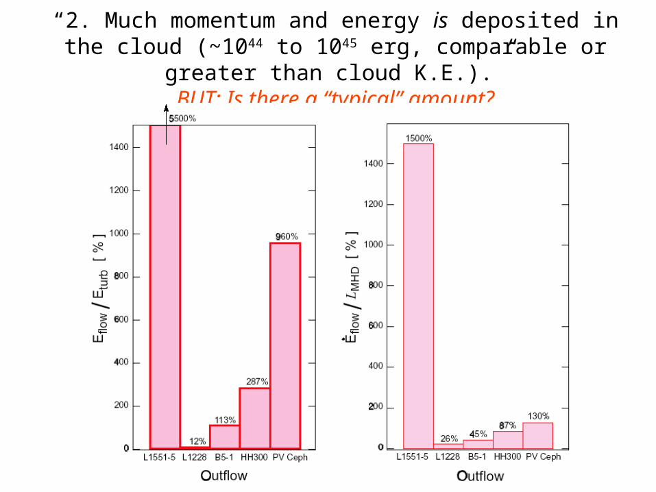
“2. Much momentum and energy is deposited in the cloud (~1044 to 1045 erg, comparable or greater than

cloud K.E.).”BUT: Is there a “typical” amount?

H. Arce’s Thesis 2001

“3. Some cloud features are all outflow. That’s how much gas is

shoved around!”

Arce & Goodman 2001; 2002

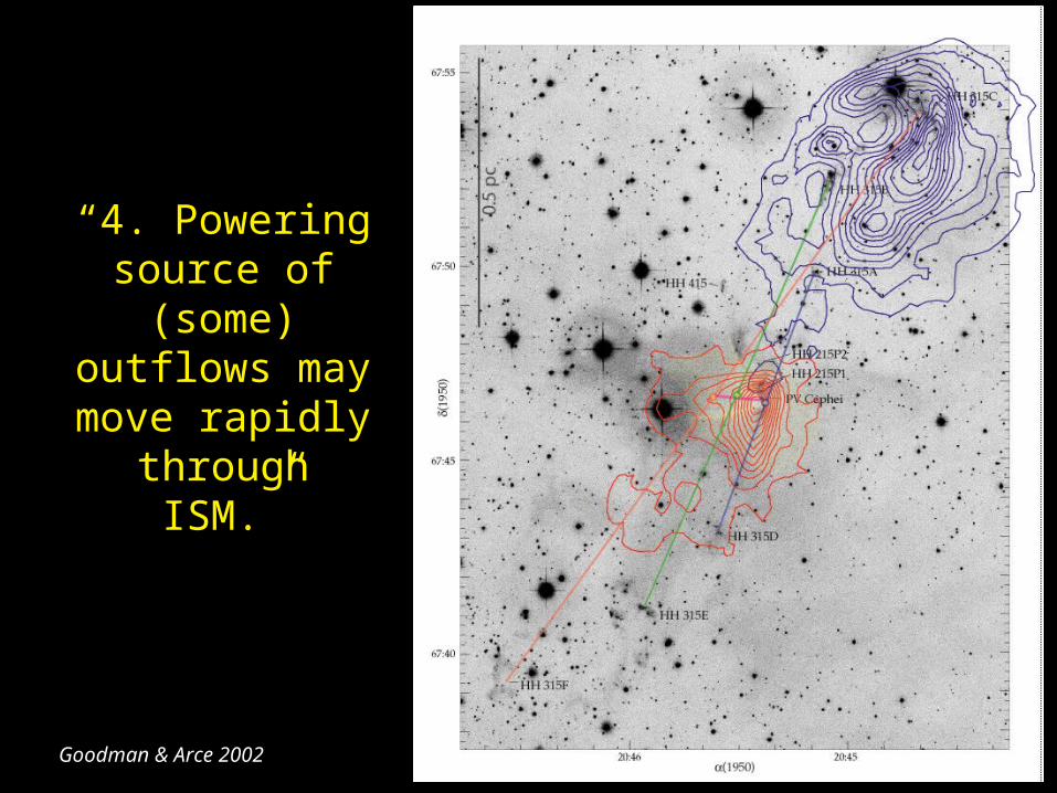
“4. Powering source of (some)

outflows may move rapidly through ISM.”

Goodman & Arce 2002

“Giant” Herbig-Haro

Flow inPV Ceph

Reipurth, Bally & Devine 1997

1 pc

PV Ceph: Episodic ejections

from precessing or

wobbling moving source

Implied source motion ~7 km/s (3 mas/year)

assuming jet velocity ~100 km/s

Goodman & Arce 2002

“4. Powering source of (some)

outflows may move rapidly through ISM.”

Goodman & Arce 2002

Goodman & Arce 2002

HST WFPC2 Overlay: Padgett et al. 2002

Arce & Goodman 2002

Goodman & Arce 2002

Trail & Jet

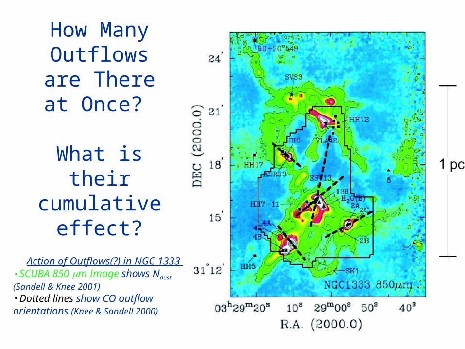
How Many Outflows are

There at Once?

What is their cumulative

effect?

How Many Outflows are

There at Once?

What is their cumulative

effect?

Action of Outflows(?) in NGC 1333 •SCUBA 850 m Image shows Ndust (Sandell & Knee 2001)•Dotted lines show CO outflow orientations (Knee & Sandell 2000)

“Beyond Now”

The COordinated Molecular Probe Line Extinction Thermal Emission Survey

Alyssa A. Goodman, Principal Investigator (CfA)João Alves (ESA, Germany)

Héctor Arce (Caltech)Paola Caselli (Arcetri, Italy)

James DiFrancesco (Berkeley)Doug Johnstone (HIA, Canada)

Scott Schnee (CfA)Mario Tafalla (OAS, Spain)Tom Wilson (MPIfR/SMTO)

“Beyond Now” The SIRTFLegacySurvey

“From Molecular Cores to Planet-Forming Disks”Neal J. Evans, II, Principal Investigator (U. Texas)

Lori E. Allen (CfA)Geoffrey A. Blake (Caltech) Paul M. Harvey (U. Texas)

David W. Koerner (U. Pennsylvania)Lee G. Mundy (Maryland)

Philip C. Myers (CfA) Deborah L. Padgett (SIRTF Science Center)

Anneila I. Sargent (Caltech)Karl Stapelfeldt (JPL)

Ewine F. van Dishoeck (Leiden)

SIRTF Legacy Survey

Perseus Molecular Cloud Complex(one of 5 similar regions to be fully mapped in far-IR by SIRTF Legacy)

SIRTF Legacy Survey

MIRAC Coverage

2 degrees ~ 10 pc

2MASS/NICER Extinction Map of Orion

Un(coordinated) Molecular-Probe Line, Extinction

and Thermal Emission

Observations

5:41:0040 20 40 42:00

2:00

55

50

05

10

15

20

25

30

R.A. (2000)

1 pc

SCUBA

5:40:003041:003042:00

2:00

1:50

10

20

30

40

R.A. (2000)

1 pc

SCUBA

Molecular Line Map

Nagahama et al. 1998 13CO (1-0) Survey

Lombardi & Alves 2001Johnstone et al. 2001 Johnstone et al. 2001

More Probes ≠ More Confusion

C18ODust EmissionOptical Image

NICER Extinction Map

Radial Density Profile, with Critical

Bonnor-Ebert Sphere Fit

Coordinated Molecular-Probe Line, Extinction & Thermal Emission Observations of Barnard 68

This figure highlights the work of Senior Collaborator João Alves and his collaborators. The top left panel shows a deep VLT image (Alves, Lada & Lada 2001). The middle top panel shows the 850 m continuum emission (Visser, Richer & Chandler 2001) from the dust causing the extinction seen optically. The top right panel highlights the extreme depletion seen at high extinctions in C18O emission (Lada et al. 2001). The inset on the bottom right panel shows the extinction map derived from applying the NICER method applied to NTT near-infrared observations of the most extinguished portion of B68. The graph in the bottom right panel shows the incredible radial-density profile derived from the NICER extinction map (Alves, Lada & Lada 2001). Notice that the fit to this profile shows the inner portion of B68 to be essentially a perfect critical Bonner-Ebert sphere

Observing Then & Now

10-4

10-3

10-2

10-1

100

101

102

103

Time (hours)

20152010200520001995199019851980

Year

1 Hour

1 Minute

1 Day

1 Second

1 Week

SCUBA-2

SEQUOIA+

NICER/8-m

NICER/SIRTFNICER/2MASS

AV~5 mag, Resolution~1'

AV~30 mag, Resolution~10"

13CO Spectra for 32 Positions in a Dark Cloud (S/N~3)

Sub-mm Map of a Dense Core at 450 and 850 m

1 day for a 13CO map then

1 minute for a 13CO map now

COMPLETE, Part 1

Observations:Mid- and Far-IR SIRTF Legacy Observations: dust temperature and column density maps ~5 degrees mapped with ~15" resolution (at 70 m)

NICER/2MASS Extinction Mapping: dust column density maps, used as target list in HHT & FCRAO observations + reddening information ~5 degrees mapped with ~5' resolution

HHT Observations: dust column density maps, finds all "cold" source ~20" resolution on all AV>2”

FCRAO/SEQUOIA 13CO and 13CO Observations: gas temperature, density and velocity information ~40" resolution on all AV>1

Science:Combined Thermal Emission (SIRTF/HHT) data: dust spectral-energy distributions, giving emissivity, Tdust and Ndust

Extinction/Thermal Emission inter-comparison: unprecedented constraints on dust properties and cloud distances, in addition to high-dynamic range Ndust map

Spectral-line/Ndust Comparisons Systematic censes of inflow, outflow & turbulent motions will be enabled—for regions with independent constraints on their density.

CO maps in conjunction with SIRTF point sources will comprise YSO outflow census

5 degrees (~tens of pc)

SIRTF Legacy Coverage of Perseus

COMPLETE, Part 2

Observations, using target list generated from Part 1:

NICER/8-m/IR camera Observations: best density profiles for dust

associated with "cores". ~10" resolution SCUBA Observations: density and temperature profiles for dust associated with "cores" ~10" resolutionFCRAO+ IRAM N2H+ Observations: gas temperature, density and velocity information for "cores” ~15" resolution

Science:Multiplicity/fragmentation studies

Detailed modeling of pressure structure on <0.3 pc scales

Searches for the "loss" of turbulent energy (coherence)

FCRAO N2H+ map with CS spectra superimposed.

(Le

e,

Mye

rs &

Ta

falla

20

01

).

Outflows

MagnetohydrodynamicWaves

Thermal Motions

MHDTurbulence

InwardMotions

SNe/GRBH II Regions

“We should not hire a star formation theorist. Star formation is too messy a problem, and will never be solved. It’s not worthy of a theorist.”

Star Formation Then and Now

1. How does one calculate the long-term efficiency of star formation in realistic galactic molecular clouds, and can that calculation explain the extragalactic “Schmidt Law”?

– Does energy injection from episodic outflows matter? – How do clouds end? Are they sheared to bits? Torn up by outflows?– Is the IMF really universal? Is it determined by turbulence alone?– Is magnetic field strength important?– How much damage do HII regions & explosions do to realistic clouds?– How long does all of this take?

The big question, and its descendants, for unworthy theorists (and observers!):

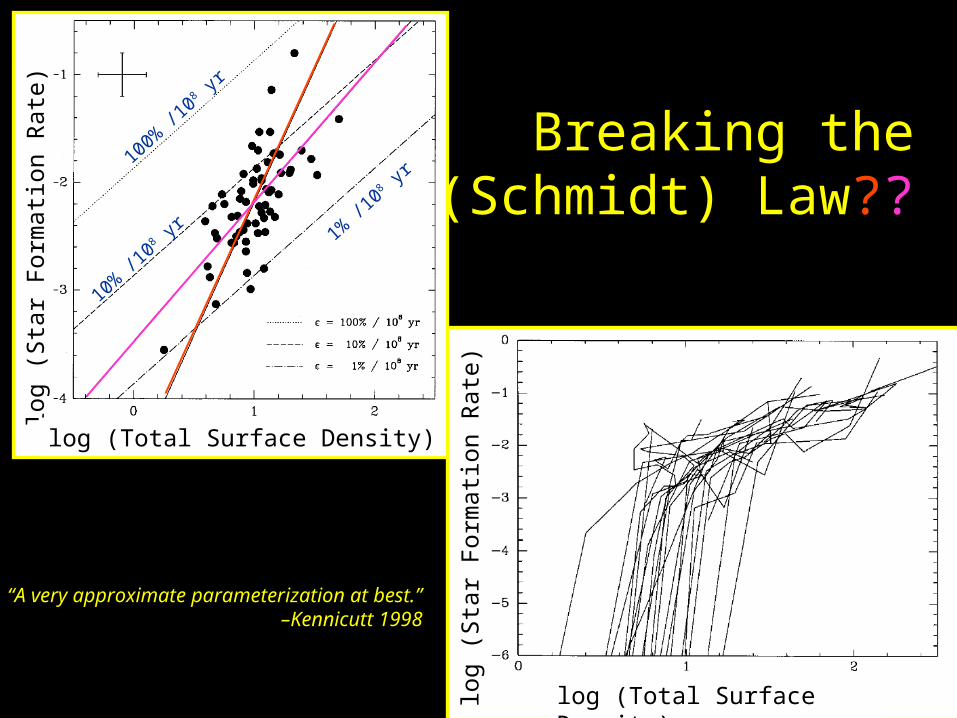
Breaking the (Schmidt) Law??

“A very approximate parameterization at best.”–Kennicutt 1998

log (

Sta

r Fo

rmati

on R

ate

)

log (Total Surface Density)lo

g (

Sta

r Fo

rmati

on R

ate

)

100%

/108 y

r

1% /1

08 y

r

10%

/108 y

r

log (Total Surface Density)