Stanley: The robot that won the DARPA Grand Challengerobots.stanford.edu/papers/thrun.stanley05.pdf · 3000 Sand Hill Road, Bldg. 3, Suite 290 ... which won the 2005 DARPA Grand Challenge

Stanley: The Robot that Wonthe DARPA Grand Challenge

Sebastian Thrun, Mike Montemerlo,Hendrik Dahlkamp, David Stavens,Andrei Aron, James Diebel, Philip Fong,John Gale, Morgan Halpenny,Gabriel Hoffmann, Kenny Lau, Celia Oakley,Mark Palatucci, Vaughan Pratt,and Pascal StangStanford Artificial Intelligence LaboratoryStanford UniversityStanford, California 94305

Sven Strohband, Cedric Dupont,Lars-Erik Jendrossek, Christian Koelen,Charles Markey, Carlo Rummel,Joe van Niekerk, Eric Jensen,and Philippe AlessandriniVolkswagen of America, Inc.Electronics Research Laboratory4009 Miranda Avenue, Suite 100Palo Alto, California 94304

Gary Bradski, Bob Davies, Scott Ettinger,Adrian Kaehler, and Ara NefianIntel Research2200 Mission College BoulevardSanta Clara, California 95052

Pamela MahoneyMohr Davidow Ventures3000 Sand Hill Road, Bldg. 3, Suite 290Menlo Park, California 94025

Received 13 April 2006; accepted 27 June 2006

• • • • • • • • • • • • • • • • • • • • • • • • • • • • • • •

Journal of Field Robotics 23(9), 661–692 (2006) © 2006 Wiley Periodicals, Inc.Published online in Wiley InterScience (www.interscience.wiley.com). • DOI: 10.1002/rob.20147

This article describes the robot Stanley, which won the 2005 DARPA Grand Challenge.Stanley was developed for high-speed desert driving without manual intervention. Therobot’s software system relied predominately on state-of-the-art artificial intelligencetechnologies, such as machine learning and probabilistic reasoning. This paper describesthe major components of this architecture, and discusses the results of the Grand Chal-lenge race. © 2006 Wiley Periodicals, Inc.

1. INTRODUCTION

The Grand Challenge was launched by the DefenseAdvanced Research Projects Agency �DARPA� in2003 to spur innovation in unmanned ground vehiclenavigation. The goal of the Challenge was to developan autonomous robot capable of traversing unre-hearsed off-road terrain. The first competition, whichcarried a prize of $1M, took place on March 13, 2004.It required robots to navigate a 142-mile long coursethrough the Mojave desert in no more than 10 h. 107teams registered and 15 raced, yet none of the par-ticipating robots navigated more than 5% of the entirecourse. The challenge was repeated on October 8,2005, with an increased prize of $2M. This time, 195teams registered and 23 raced. Of those, five teamsfinished. Stanford’s robot “Stanley” finished thecourse ahead of all other vehicles in 6 h, 53 min, and58 s, and was declared the winner of the DARPAGrand Challenge; see Figure 1.

This paper describes the robot Stanley, and itssoftware system in particular. Stanley was developedby a team of researchers to advance the state-of-the-art in autonomous driving. Stanley’s success is the re-

sult of an intense development effort led by StanfordUniversity, and involving experts from Volkswagenof America, Mohr Davidow Ventures, Intel Research,and a number of other entities. Stanley is based on a2004 Volkswagen Touareg R5 TDI, outfitted with a sixprocessor computing platform provided by Intel, anda suite of sensors and actuators for autonomous driv-ing. Figure 2 shows images of Stanley during the race.

The main technological challenge in the develop-ment of Stanley was to build a highly reliable system,capable of driving at relatively high speeds throughdiverse and unstructured off-road environments, andto do all this with high precision. These requirementsled to a number of advances in the field of autono-mous navigation, as surveyed in this paper. Methodswere developed, and existing methods extended, inthe areas of long-range terrain perception, real-timecollision avoidance, and stable vehicle control on slip-pery and rugged terrain. Many of these develop-ments were driven by the speed requirement, whichrendered many classical techniques in the off-roaddriving field unsuitable. In pursuing these develop-ments, the research team brought to bear algorithms

Figure 1. �a� At approximately 1:40 pm on Oct 8, 2005, Stanley was the first robot to complete the DARPA GrandChallenge. �b� The robot is being honored by DARPA Director Dr. Tony Tether.

662 • Journal of Field Robotics—2006

Journal of Field Robotics DOI 10.1002/rob

from diverse areas including distributed systems,machine learning, and probabilistic robotics.

1.1. Race Rules

The rules �DARPA, 2004� of the DARPA Grand Chal-lenge were simple. Contestants were required tobuild autonomous ground vehicles capable of tra-versing a desert course up to 175-miles long in lessthan 10 h. The first robot to complete the course inunder 10 h would win the challenge and the $2Mprize. Absolutely no manual intervention was al-lowed. The robots were started by DARPA personneland from that point on had to drive themselves.Teams only saw their robots at the starting line and,with luck, at the finish line.

Both the 2004 and 2005 races were held in theMojave desert in the southwest United States. Thecourse terrain varied from high-quality graded dirtroads to winding rocky mountain passes; see Figure2. A small fraction of each course traveled alongpaved roads. The 2004 course started in Barstow,

CA, approximately 100 miles northeast of Los Ange-les, and finished in Primm, NV, approximately30 miles southwest of Las Vegas. The 2005 courseboth started and finished in Primm, NV.

The specific race course was kept secret from allteams until 2 h before the race. At this time, eachteam was given a description of the course on CD-ROM in a DARPA-defined route definition data for-mat �RDDF�. The RDDF is a list of longitudes, lati-tudes, and corridor widths that define the courseboundary, and a list of associated speed limits; anexample segment is shown in Figure 3. Robots thattravel substantially beyond the course boundary riskdisqualification. In the 2005 race, the RDDF con-tained 2,935 waypoints.

The width of the race corridor generally trackedthe width of the road, varying between 3 and 30 min the 2005 race. Speed limits were used to protectimportant infrastructure and ecology along thecourse, and to maintain the safety of DARPA chasedrivers who followed behind each robot. The speedlimits varied between 5 and 50 mph. The RDDF de-fined the approximate route that robots would take,

Figure 2. Images from the race.

Figure 3. A section of the RDDF file from the 2005DARPA Grand Challenge. The corridor varies in widthand maximum speed. Waypoints are more frequent inturns.

Thrun et al.: Stanley: The Robot that Won • 663


so no global path planning was required. As a result,the race was primarily a test of high-speed roadfinding, obstacle detection, and avoidance in desertterrain.

The robots all competed on the same course;starting one after another at 5 min intervals. When afaster robot overtook a slower one, the slower robotwas paused by DARPA officials, allowing the secondrobot to pass the first as if it were a static obstacle.This eliminated the need for robots to handle thecase of dynamic passing.

1.2. Team Composition

The Stanford Racing Team team was organized intofour major groups. The Vehicle Group oversaw allmodifications and component developments relatedto the core vehicle. This included the drive-by-wiresystems, the sensor and computer mounts, and thecomputer systems. The group was led by researchersfrom Volkswagen of America’s Electronics ResearchLab. The Software Group developed all software, in-cluding the navigation software and the varioushealth monitor and safety systems. The softwaregroup was led by researchers affiliated with Stan-ford University. The Testing Group was responsiblefor testing all system components and the system asa whole, according to a specified testing schedule.The members of this group were separate from anyof the other groups. The testing group was led byresearchers affiliated with Stanford University. TheCommunications Group managed all media relationsand fund raising activities of the Stanford RacingTeam. The communications group was led by em-ployees of Mohr Davidow Ventures, with participa-tion from all other sponsors. The operations over-sight was provided by a steering board that includedall major supporters.

2. VEHICLE

Stanley is based on a diesel-powered VolkswagenTouareg R5. The Touareg has four-wheel drive�4WD�, variable-height air suspension, and automaticelectronic locking differentials. To protect the vehiclefrom environmental impact, Stanley has been outfit-ted with skid plates and a reinforced front bumper. Acustom interface enables direct electronic actuation ofboth the throttle and brakes. A DC motor attached tothe steering column provides electronic steering con-trol. A linear actuator attached to the gear shiftershifts the vehicle between drive, reverse, and parkinggears �Figure 4�c��. Vehicle data, such as individualwheel speeds and steering angle, are sensed auto-matically and communicated to the computer systemthrough a CAN bus interface.

The vehicle’s custom-made roof rack is shown inFigure 4�a�. It holds nearly all of Stanley’s sensors.The roof provides the highest vantage point of the ve-hicle; from this point, the visibility of the terrain isbest, and the access to global positioning system�GPS� signals is least obstructed. For environmentperception, the roof rack houses five SICK laser rangefinders. The lasers are pointed forward along thedriving direction of the vehicle, but with slightly dif-ferent tilt angles. The lasers measure cross sections ofthe approaching terrain at different ranges out to25 m in front of the vehicle. The roof rack also holdsa color camera for long-range road perception, whichis pointed forward and angled slightly downward.For long-range detection of large obstacles, Stanley’sroof rack also holds two 24 GHz RADAR sensors,supplied by Smart Microwave Sensors. Both RADARsensors cover the frontal area up to 200 m, with a cov-erage angle in azimuth of about 20°. Two antennae ofthis system are mounted on both sides of the lasersensor array. The lasers, camera, and radar system

Figure 4. �a� View of the vehicle’s roof rack with sensors. �b� The computing system in the trunk of the vehicle. �c� Thegear shifter, control screen, and manual override buttons.



comprise the environment sensor group of the system.That is, they inform Stanley of the terrain ahead, sothat Stanley can decide where to drive, and at whatspeed.

Further back, the roof rack holds a number of ad-ditional antennae: One for Stanley’s GPS positioningsystem and two for the GPS compass. The GPS po-sitioning unit is a L1/L2/Omnistar HP receiver. To-gether with a trunk-mounted inertial measurementunit �IMU�, the GPS systems are the positioning sensorgroup, whose primary function is to estimate the lo-cation and velocity of the vehicle relative to an exter-nal coordinate system.

Finally, a radio antenna and three additional GPSantennae from the DARPA E-Stop system are also lo-cated on the roof. The E-Stop system is a wireless linkthat allows a chase vehicle following Stanley to safelystop the vehicle in case of emergency. The roof rackalso holds a signaling horn, a warning light, and twomanual E-stop buttons.

Stanley’s computing system is located in the ve-hicle’s trunk, as shown in Figure 4�b�. Special airducts direct air flow from the vehicle’s air condition-ing system into the trunk for cooling. The trunk fea-tures a shock-mounted rack that carries an array ofsix Pentium M computers, a Gigabit Ethernet switch,and various devices that interface to the physical sen-sors and the Touareg’s actuators. It also features acustom-made power system with backup batteries,and a switch box that enables Stanley to power-cycleindividual system components through software.The DARPA-provided E-Stop is located on this rackon additional shock compensation. The trunk assem-bly also holds the custom interface to the VolkswagenTouareg’s actuators: The brake, throttle, gear shifter,and steering controller. A six degree-of-freedom IMUis rigidly attached to the vehicle frame underneaththe computing rack in the trunk.

The total power requirement of the added instru-mentation is approximately 500 W, which is pro-vided through the Touareg’s stock alternator. Stan-ley’s backup battery system supplies an additionalbuffer to accommodate long idling periods in desertheat.

The operating system run on all computers isLinux. Linux was chosen due to its excellent network-ing and time sharing capabilities. During the race,Stanley executed the race software on three of the sixcomputers; a fourth was used to log the race data�and two computers were idle�. One of the three racecomputers was entirely dedicated to video process-

ing, whereas the other two executed all other soft-ware. The computers were able to poll the sensors atup to 100 Hz, and to control the steering, throttle andbrake at frequencies up to 20 Hz.

An important aspect in Stanley’s design was toretain street legality, so that a human driver couldsafely operate the robot as a conventional passengercar. Stanley’s custom user interface enables a driver toengage and disengage the computer system at will,even while the vehicle is in motion. As a result, thedriver can disable computer control at any time of thedevelopment, and regain manual control of the ve-hicle. To this end, Stanley is equipped with severalmanual override buttons located near the driver seat.Each of these switches controls one of the three majoractuators �brakes, throttle, and steering�. An addi-tional central emergency switch disengages all com-puter control and transforms the robot into a conven-tional vehicle. While this feature was of no relevanceto the actual race �in which no person sat in the car�,it proved greatly beneficial during software develop-ment. The interface made it possible to operate Stan-ley autonomously with people inside, as a dedicatedsafety driver could always catch computer glitchesand assume full manual control at any time.

During the actual race, there was of course nodriver in the vehicle, and all driving decisions weremade by Stanley’s computers. Stanley possessed anoperational control interface realized through atouch-sensitive screen on the driver’s console. Thisinterface allowed Government personnel to shutdown and restart the vehicle, if it became necessary.

3. SOFTWARE ARCHITECTURE

3.1. Design Principles

Before both the 2004 and 2005 Grand Challenges,DARPA revealed to the competitors that a stock4WD pickup truck would be physically capable oftraversing the entire course. These announcementssuggested that the innovations necessary to success-fully complete the challenge would be in designingintelligent driving software, not in designing exoticvehicles. This announcement and the performance ofthe top finishers in the 2004 race guided the designphilosophy of the Stanford Racing Team: Treat au-tonomous navigation as a software problem.



In relation to previous work on robotics architec-tures, Stanley’s software architecture is related to thewell-known three-layer architecture �Gat, 1998�, albeitwithout a long-term symbolic planning method. Anumber of guiding principles proved essential in thedesign of the software architecture:

3.1.1. Control and Data Pipeline

There is no centralized master process in Stanley’ssoftware system. All modules are executed at theirown pace, without interprocess synchronizationmechanisms. Instead, all data are globally timestamped, and time stamps are used when integrat-ing multiple data sources. The approach reduces therisk of deadlocks and undesired processing delays.To maximize the configurability of the system,nearly all interprocess communication is imple-mented through publish-subscribe mechanisms. Theinformation from sensors to actuators flows in asingle direction; no information is received morethan once by the same module. At any point in time,all modules in the pipeline are working simulta-neously, thereby maximizing the informationthroughput and minimizing the latency of the soft-ware system.

3.1.2. State Management

Even though the software is distributed, the state ofthe system is maintained by local authorities. Thereare a number of state variables in the system. Thehealth state is locally managed in the health monitor;the parameter state in the parameter server; the glo-bal driving mode is maintained in a finite state au-tomaton; and the vehicle state is estimated in thestate estimator module. The environment state isbroken down into multiple maps �laser, vision, andradar�. Each of these maps are maintained in dedi-cated modules. As a result, all other modules willreceive values that are mutually consistent. The ex-act state variables are discussed in later sections ofthis paper. All state variables are broadcast to rel-evant modules of the software system through apublish-subscribe mechanism.

3.1.3. Reliability

The software places strong emphasis on the overallreliability of the robotic system. Special modulesmonitor the health of individual software and hard-

ware components, and automatically restart orpower-cycle such components when a failure is ob-served. In this way, the software is robust to certainoccurrences, such as crashing or hanging of a soft-ware modules or stalled sensors.

3.1.4. Development Support

Finally, the software is structured so as to aid devel-opment and debugging of the system. The developercan easily run just a subsystem of the software, andeffortlessly migrate modules across different proces-sors. To facilitate debugging during the develop-ment process, all data are logged. By using a specialreplay module, the software can be run on recordeddata. A number of visualization tools were devel-oped that make it possible to inspect data and inter-nal variables while the vehicle is in motion, or whilereplaying previously logged data. The developmentprocess used a version control process with a strictset of rules for the release of race-quality software.Overall, we found that the flexibility of the softwareduring development was essential in achieving thehigh level of reliability necessary for long-term au-tonomous operation.

3.2. Processing Pipeline

The race software consisted of approximately 30modules executed in parallel �Figure 5�. The systemis broken down into six layers which correspond tothe following functions: Sensor interface, perception,control, vehicle interface, user interface, and globalservices.

1. The sensor interface layer comprises a num-ber of software modules concerned with re-ceiving and time stamping all sensor data.The layer receives data from each laser sensorat 75 Hz, from the camera at approximately12 Hz, the GPS and GPS compass at 10 Hz,and the IMU and the Touareg CAN bus at100 Hz. This layer also contains a databaseserver with the course coordinates �RDDFfile�.

2. The perception layer maps sensor data intointernal models. The primary module in thislayer is the unscented Kalman filter �UKF�vehicle state estimator, which determines thevehicle’s coordinates, orientation, and veloci-ties. Three different mapping modules build



two-dimensional �2D� environment mapsbased on lasers, the camera, and the radarsystem. A road finding module uses the laser-derived maps to find the boundary of a road,so that the vehicle can center itself laterally.Finally, a surface assessment module extractsparameters of the current road for the pur-pose of determining safe vehicle speeds.

3. The control layer is responsible for regulat-ing the steering, throttle, and brake responseof the vehicle. A key module is the path plan-ner, which sets the trajectory of the vehicle insteering and velocity space. This trajectory ispassed to two closed-loop trajectory tracking

controllers, one for the steering control andone for brake and throttle control. Both con-trollers send low-level commands to the ac-tuators that faithfully execute the trajectoryemitted by the planner. The control layer alsofeatures a top level control module, imple-mented as a simple finite state automaton.This level determines the general vehiclemode in response to user commands receivedthrough the in-vehicle touch screen or thewireless E-stop, and maintains gear state incase backward motion is required.

4. The vehicle interface layer serves as the in-terface to the robot’s drive-by-wire system. It

Figure 5. Flowchart of Stanley software system. The software is roughly divided into six main functional groups: Sensorinterface, perception, control, vehicle interface, and user interface. There are a number of cross-cutting services, such asthe process controller and the logging modules.



contains all interfaces to the vehicle’s brakes,throttle, and steering wheel. It also featuresthe interface to the vehicle’s server, a circuitthat regulates the physical power to many ofthe system components.

5. The user interface layer comprises the re-mote E-stop and a touch-screen module forstarting up the software.

6. The global services layer provides a numberof basic services for all software modules.Naming and communication services areprovides through Carnegie Mellon Universi-ty’s �CMU’s� interprocess communicationtoolkit �Simmons & Apfelbaum, 1998�. A cen-tralized parameter server maintains a data-base of all vehicle parameters and updatesthem in a consistent manner. The physicalpower of individual system components isregulated by the power server. Another mod-ule monitors the health of all systems com-ponents and restarts individual system com-ponents when necessary. Clock synchron-ization is achieved through a time server. Fi-nally, a data logging server dumps sensor,control, and diagnostic data to disk for replayand analysis.

The following sections will describe Stanley’s coresoftware processes in greater detail. The paper willthen conclude with a description of Stanley’s perfor-mance in the Grand Challenge.

4. VEHICLE STATE ESTIMATION

Estimating vehicle state is a key prerequisite for pre-cision driving. Inaccurate pose estimation can causethe vehicle to drive outside the corridor, or build ter-rain maps that do not reflect the state of the robot’senvironment, leading to poor driving decisions. InStanley, the vehicle state comprises a total of 15 vari-ables. The design of this parameter space followsstandard methodology �Farrell & Barth, 1999; van derMerwe & Wan, 2004�, as indicated in Table I.

An unscented Kalman filter �UKF� �Julier & Uhl-mann, 1997� estimates these quantities at an updaterate of 100 Hz. The UKF incorporates observationsfrom the GPS, the GPS compass, the IMU, and thewheel encoders. The GPS system provides both ab-solute position and velocity measurements, which areboth incorporated into the UKF. From a mathematical

point of view, the sigma point linearization in theUKF often yields a lower estimation error than thelinearization based on Taylor expansion in the ex-tended Kalman filter �EKF� �van der Merwe, 2004�. Tomany, the UKF is also preferable from an implemen-tation standpoint because it does not require the ex-plicit calculation of any Jacobians; although those canbe useful for further analysis.

While GPS is available, the UKF uses only a“weak” model. This model corresponds to a movingmass that can move in any direction. Hence, in nor-mal operating mode, the UKF places no constraint onthe direction of the velocity vector relative to the ve-hicle’s orientation. Such a model is clearly inaccurate,but the vehicle-ground interactions in slippery desertterrain are generally difficult to model. The movingmass model allows for any slipping or skidding thatmay occur during off-road driving.

However, this model performs poorly duringGPS outages, as the position of the vehicle reliesstrongly on the accuracy of the IMU’s accelerometers.As a consequence, a more restrictive UKF motionmodel is used during GPS outages. This model con-strains the vehicle to only move in the direction it ispointed. The integration of the IMU’s gyroscopes fororientation, coupled with wheel velocities for com-puting the position, is able to maintain accurate poseof the vehicle during GPS outages of up to 2 minlong; the accrued error is usually in the order of cen-timeters. Stanley’s health monitor will decrease themaximum vehicle velocity during GPS outages to10 mph in order to maximize the accuracy of the re-stricted vehicle model. Figure 6�a� shows the result ofposition estimation during a GPS outage with theweak vehicle model; Figure 6�b�, the result with thestrong vehicle model. This experiment illustrates theperformance of this filter during a GPS outage.Clearly, accurate vehicle modeling during GPS out-

Table I. Standard methodology of Stanley’s 15 variables.

No. of values State variable

3 Position �longitude, latitude, and altitude�3 Velocity

3 Orientation �Euler angles: roll, pitch,and yaw�

3 Accelerometer biases

3 Gyro biases



ages is essential. In an experiment on a paved road,we found that even after 1.3 km of travel withoutGPS on a cyclic course, the accumulated vehicle errorwas only 1.7 m.

5. LASER TERRAIN MAPPING

5.1. Terrain Labeling

To safely avoid obstacles, Stanley must be capable ofaccurately detecting nondrivable terrain at a suffi-cient range to stop or take the appropriate evasiveaction. The faster the vehicle is moving, the fartheraway obstacles must be detected. Lasers are used asthe basis for Stanley’s short and medium range ob-

stacle avoidance. Stanley is equipped with fivesingle-scan laser range finders mounted on the roof,tilted downward to scan the road ahead. Figure 7�a�illustrates the scanning process. Each laser scan gen-erates a vector of 181 range measurements spaced0.5° apart. Projecting these scans into the global co-ordinate frame according, to the estimated pose ofthe vehicle, results in a 3D point cloud for each laser.Figure 7�b� shows an example of the point cloudsacquired by the different sensors. The coordinates ofsuch 3D points are denoted �Xk

i Yki Zk

i �; where k is thetime index at which the point was acquired, and i isthe index of the laser beam.

Obstacle detection on laser point clouds can beformulated as a classification problem, assigning toeach 2D location in a surface grid one of three pos-sible values: Occupied, free, and unknown. A loca-tion is occupied by an obstacle if we can find twonearby points whose vertical distance �Zk

i −Zmj � ex-

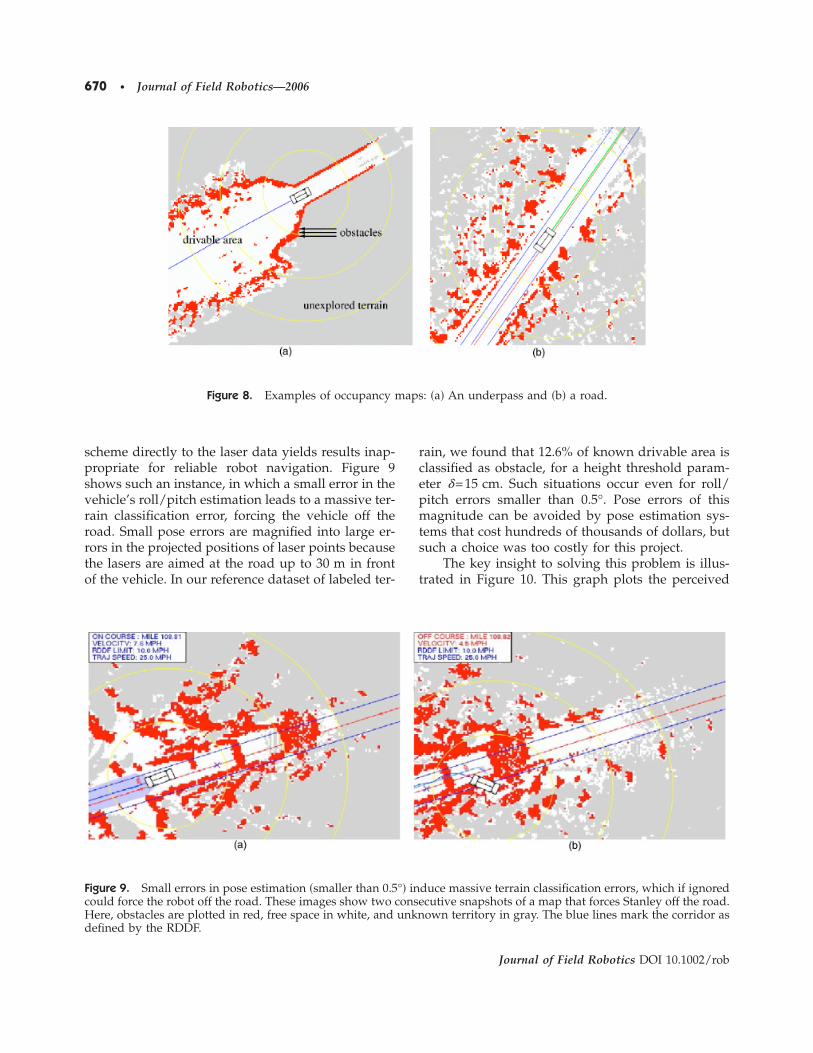
ceeds a critical vertical distance �. It is considereddrivable �free of obstacles� if no such points can befound, but at least one of the readings falls into thecorresponding grid cell. If no reading falls into thecell, the drivability of this cell is considered un-known. The search for nearby points is convenientlyorganized in a 2D grid, the same grid used as thefinal drivability map that is provided to the vehicle’snavigation engine. Figure 8 shows the example gridmap. As indicated in this figure, the map assignsterrain to one of three classes: Drivable, occupied, orunknown.

Unfortunately, applying this classification

Figure 6. UKF state estimation when GPS becomes un-available. The area covered by the robot is approximately100�100 m. The large ellipses illlustrate the position un-certainty after losing GPS. �a� Without integrating thewheel motion the result is highly erroneous. �b� The wheelmotion clearly improves the result.

Figure 7. �a� Illustration of a laser sensor: The sensor is angled downward to scan the terrain in front of the vehicle as itmoves. Stanley possesses five such sensors, mounted at five different angles. �b� Each laser acquires a three-dimensional�3D� point cloud over time. The point cloud is analyzed for drivable terrain and potential obstacles.



scheme directly to the laser data yields results inap-propriate for reliable robot navigation. Figure 9shows such an instance, in which a small error in thevehicle’s roll/pitch estimation leads to a massive ter-rain classification error, forcing the vehicle off theroad. Small pose errors are magnified into large er-rors in the projected positions of laser points becausethe lasers are aimed at the road up to 30 m in frontof the vehicle. In our reference dataset of labeled ter-

rain, we found that 12.6% of known drivable area isclassified as obstacle, for a height threshold param-eter �=15 cm. Such situations occur even for roll/pitch errors smaller than 0.5°. Pose errors of thismagnitude can be avoided by pose estimation sys-tems that cost hundreds of thousands of dollars, butsuch a choice was too costly for this project.

The key insight to solving this problem is illus-trated in Figure 10. This graph plots the perceived

Figure 8. Examples of occupancy maps: �a� An underpass and �b� a road.

Figure 9. Small errors in pose estimation �smaller than 0.5°� induce massive terrain classification errors, which if ignoredcould force the robot off the road. These images show two consecutive snapshots of a map that forces Stanley off the road.Here, obstacles are plotted in red, free space in white, and unknown territory in gray. The blue lines mark the corridor asdefined by the RDDF.



obstacle height �Zki −Zm

j � along the vertical axis for acollection of grid cells taken from flat terrain.Clearly, for some grid cells, the perceived height isenormous—despite the fact that in reality, the sur-face is flat. However, this function is not random.The horizontal axis depicts the time difference �t�k−m� between the acquisition of those scans. Obvi-ously, the error is strongly correlated with theelapsed time between the two scans.

To model this error, Stanley uses a first-orderMarkov model, which models the drift of the poseestimation error over time. The test for the presenceof an obstacle is therefore a probabilistic test. Giventwo points �Xk

i Yki Zk

i �T and �Xmj Ym

j Zmj �T, the height

difference is distributed according to a normal dis-tribution whose variance scales linearly with thetime difference �k−m�. Thus, Stanley uses a probabi-listic test for the presence of an obstacle, of the type

p��Zki − Zm

j � � �� , �1�

where � is a confidence threshold, e.g., �=0.05.When applied over a 2D grid, the probabilistic

method can be implemented efficiently so that onlytwo measurements have to be stored per grid cell.This is due to the fact that each measurement definesa bound on future Z values for obstacle detection.For example, suppose we observe a measurement

for a cell which was previously observed. Then, oneor more of three cases will be true:

1. The measurement might be a witness of anobstacle, according to the probabilistic test. Inthis case, Stanley simply marks the cell as anobstacle and no further testing takes place.

2. The measurement does not trigger as a wit-ness of an obstacle; but, in future tests, it es-tablishes a tighter lower bound on the mini-mum Z value than the previously storedmeasurement. In this case, our algorithmsimply replaces the previous measurementwith this one. The rationale behind this issimple: If the measurement is more restrictivethan the previous one, there will not be a situ-ation where a test against this point wouldfail, while a test against the older one wouldsucceed. Hence, the old point can safely bediscarded.

3. The third case is equivalent to the second, butwith a refinement of the upper value. A mea-surement may simultaneously refine thelower and the upper bounds.

The fact that only two measurements per grid cellhave to be stored renders this algorithm highly effi-cient in space and time.

5.2. Data-Driven Parameter Tuning

A final step in developing this mapping algorithmaddresses parameter tuning. Our approach and theunderlying probabilistic Markov model possess anumber of unknown parameters. These parametersinclude the height threshold �, the statistical accep-tance probability threshold �, and various Markovchain error parameters �the noise covariances of theprocess noise and the measurement noise�.

Stanley uses a discriminative learning algorithmfor locally optimizing these parameters. This algo-rithm tunes the parameters in a way that maximizesthe discriminative accuracy of the resulting terrainanalysis on labeled training data.

The data are labeled through human driving,similar in spirit to Pomerleau �1993�. Figure 11 illus-trates the idea: A human driver is instructed to onlydrive over obstacle-free terrain. Grid cells traversedby the vehicle are then labeled as drivable: This areacorresponds to the blue stripe in Figure 11. A stripeto the left and right of this corridor is assumed to be

Figure 10. Correlation of time and vertical measurementerror in the laser data analysis.



all obstacles, as indicated by the red stripes in Figure11. The distance between the drivable and obstacle isset by hand, based on the average road width for asegment of data. Clearly, not all of those cells labeledas obstacles are actually occupied by obstacles; how-ever, even training against an approximate labelingis enough to improve the overall performance of themapper.

The learning algorithm is now implementedthrough coordinate ascent. In the outer loop, the al-gorithm performs coordinate ascent relative to adata-driven scoring function. Given an initial guess,the coordinate ascent algorithm modifies each pa-rameter one after another by a fixed amount. It thendetermines if the new value constitutes an improve-ment over the previous value when evaluated over alogged data set, and retains it accordingly. If for agiven interval size no improvement can be found,the search interval is cut in half and the search iscontinued, until the search interval becomes smallerthan a preset minimum search interval �at whichpoint the tuning is terminated�.

The probabilistic analysis, paired with the dis-criminative algorithm for parameter tuning, has asignificant effect on the accuracy of the terrain labels.Using an independent testing data set, we find thatthe false positive rate �the area labeled as drivable inFigure 11� drops from 12.6% to 0.002%. At the same

time, the rate at which the area off the road is labeledas an obstacle remains approximately constant �from22.6% to 22.0%�. This rate is not 100%, simply be-cause most of the terrain there is still flat and driv-able. Our approach for data acquisition mislabels theflat terrain as nondrivable. Such mislabeling how-ever, does not interfere with the parameter tuningalgorithm, and hence is preferable to the tediousprocess of labeling pixels manually.

Figure 12 shows an example of the mapper inaction. A snapshot of the vehicle from the side illus-trates that a part of the surface is scanned multipletimes due to a change of pitch. As a result, the non-probabilistic method hallucinates a large occupiedarea in the center of the road, shown in panel �c� ofFigure 12. Our probabilistic approach overcomes thiserror and generates a map that is good enough fordriving. A second example is shown in Figure 13.

6. COMPUTER VISION TERRAIN ANALYSIS

The effective maximum range at which obstacles canbe detected with the laser mapper is approximately22 m. This range is sufficient for Stanley to reliablyavoid obstacles at speeds up to 25 mph. Based on the2004 Race Course, the development team estimatedthat Stanley would need to reach speeds of 35 mph inorder to successfully complete the challenge. To ex-tend the sensor range enough to allow safe driving at35 mph, Stanley uses a color camera to find drivablesurfaces at ranges exceeding that of the laser analysis.Figure 14 compares laser and vision mapping side byside. The left diagram shows a laser map acquiredduring the race; here, obstacles are detected at an ap-proximate 22 m range. The vision map for the samesituation is shown on the right side. This map extendsbeyond 70 m �each yellow circle corresponds to 10 mrange�.

Our work builds on a long history of research onroad finding �Pomerleau, 1991; Crisman & Thorpe,1993�; see also Dickmanns �2002�. To find the road, thevision module classifies images into drivable andnondrivable regions. This classification task is gener-ally difficult, as the road appearance is affected by anumber of factors that are not easily measured andchange over time, such as the surface material of theroad, lighting conditions, dust on the lens of the cam-era, and so on. This suggests that an adaptive ap-proach is necessary, in which the image interpretationchanges as the vehicle moves and conditions change.

Figure 11. Terrain labeling for parameter tuning: Thearea traversed by the vehicle is labeled as “drivable”�blue� and two stripes at a fixed distance to the left and theright are labeled as “obstacles” �red�. While these labelsare only approximate, they are extremely easy to obtainand significantly improve the accuracy of the resultingmap when used for parameter tuning.



The camera images are not the only source of in-formation about upcoming terrain available to the vi-sion mapper. Although we are interested in using vi-sion to classify the drivability of terrain beyond thelaser range, we already have such drivability infor-mation from the laser in the near range. All that is re-

quired from the vision routine is to extend the reachof the laser analysis. This is different from thegeneral-purpose image interpretation problem, inwhich no such data would be available.

Stanley finds drivable surfaces by projectingdrivable area from the laser analysis into the camera

Figure 12. Example of pitching combined with small pose estimation errors: �a� The reading of the center beam of one ofthe lasers, integrated over time �some of the terrain is scanned twice.�; �b� shows 3D point cloud; �c� resulting map withoutprobabilistic analysis, and �d� map with probabilistic analysis. The map shown in �c� possesses a phantom obstacle, largeenough to force the vehicle off the road.

Figure 13. A second example of pitching combined with small page estimation errors.



image. More specifically, Stanley extracts a quadrilat-eral ahead of the robot in the laser map, so that allgrid cells within this quadrilateral are drivable. Therange of this quadrilateral is typically between 10 and20 m ahead of the robot. An example of such a quad-rilateral is shown in Figure 14�a�. Using straightfor-ward geometric projection, this quadrilateral is thenmapped into the camera image, as illustrated in Fig-ures 15�a� and 15�b�. An adaptive computer vision al-gorithm then uses the image pixels inside this quad-rilateral as training examples for the concept ofdrivable surface.

The learning algorithm maintains a mixture ofGaussians that model the color of drivable terrain.Each such mixture is a Gaussian defined in the red/green/blue �RGB� color space of individual pixels;the total number of Gaussians is denoted as n. Foreach mixture, the learning algorithm maintains a

mean RGB color �i, a covariance �i, and a count mi ofthe total number of image pixels that were used totrain this Gaussian.

When a new image is observed, the pixels in thedrivable quadrilateral are mapped into a smallernumber of k “local” Gaussians using the EM algo-rithm �Duda & Hart, 1973�, with k�n �the covarianceof these local Gaussians are inflated by a small valueso as to avoid overfitting�. These k local Gaussians arethen merged into the memory of the learning algo-rithm, in a way that allows for slow and fast adap-tation. The learning adapts to the image in two pos-sible ways; by adjusting the previously foundinternal Gaussian to the actual image pixels, and byintroducing new Gaussians and discarding olderones. Both adaptation steps are essential. The first en-ables Stanley to adapt to slowly changing lighting

Figure 14. Comparison of the laser-based �left� and the image-based �right� mapper. For scale, circles are spaced aroundthe vehicle at a 10 m distance. This diagram illustrates that the reach of lasers is approximately 22 m, whereas the visionmodule often looks 70 m ahead.

Figure 15. This figure illustrates the processing stages of the computer vision system: �a� a raw image; �b� the processedimage with the laser quadrilateral and a pixel classification; �c� the pixel classification before thresholding; and �d� horizondetection for sky removal.



conditions; the second makes it possible to adapt rap-idly to a new surface color �e.g., when Stanley movesfrom a paved to an unpaved road�.

In detail, to update the memory, consider the jthlocal Gaussian. The learning algorithm determinesthe closest Gaussian in the global memory, wherecloseness is determined through the Mahalanobisdistance

d�i,j� = ��i − �j�T��i + �j�−1��i − �j� . �2�

Let i be the index of the minimizing Gaussian in thememory. The learning algorithm then chooses one oftwo possible outcomes:

1. The distance d�i , j�, where is an accep-tance threshold. The learning algorithm thenassumes that the global Gaussian j is repre-sentative of the local Gaussian i, and adap-tation proceeds slowly. The parameters ofthis global Gaussian are set to the weightedmean:

�i ←mi�i

mi + mj+

mj�j

mi + mj, �3�

�i ←mi�i

mi + mj+

mj�j

mi + mj, �4�

mi ← mi + mj, �5�

where mj is the number of pixels in the imagethat correspond to the jth Gaussian.

2. The distance d�i , j�� for any Gaussian i inthe memory. This is the case when none of theGaussian in memory are near the localGaussian extracted form the image, wherenearness is measured by the Mahalanobisdistance. The algorithm then generates a newGaussian in the global memory, with param-eters �j, �j, and mj. If all n slots are alreadytaken in the memory, the algorithm “forgets”the Gaussian with the smallest total pixelcount mi, and replaces it by the new localGaussian.

After this step, each counter mi in the memory is dis-counted by a factor of ��1. This exponential decay

term makes sure that the Gaussians in memory can bemoved in new directions as the appearance of thedrivable surface changes over time.

For finding the drivable surface, the learnedGaussians are used to analyze the image. The imageanalysis uses an initial sky removal step defined inEttinger, Nechyba, Ifju & Waszak �2003�. A subse-quent flood-fill step then removes additional sky pix-els not found by the algorithm in Ettinger et al. �2003�.The remaining pixels are than classified using thelearned mixture of Gaussian, in the straightforwardway. Pixels whose RGB value is near one or more ofthe learned Gaussians are classified as drivable; allother pixels are flagged as nondrivable. Finally, onlyregions connected to the laser quadrilateral are la-beled as drivable.

Figure 15 illustrates the key processing steps.Panel �a� in this figure shows a raw camera image,and panel �b� shows the image after processing. Pix-els classified as drivable are colored red, whereasnondrivable pixels are colored blue. The remainingtwo panels in Figure 15 show intermediate process-ing steps: The classification response before thresh-olding �panel �c�� and the result of the sky finder�panel �d��.

Due to the ability to create new Gaussians on thefly, Stanley’s vision routine can adapt to new terrainwithin seconds. Figure 16 shows data acquired at theNational Qualification Event �NQE� of the DARPAGrand Challenge. Here the vehicle moves from thepavement to grass, both of which are drivable. Thesequence in Figure 16 illustrates the adaptation atwork: The boxed areas toward the bottom of the im-age are the training region, and the red coloring in theimage is the result of applying the learned classifier.As is easily seen in Figure 16, the vision module suc-cessfully adapts from pavement to grass within lessthan 1 s, while still correctly labeling the hay balesand other obstacles.

Under slowly changing lighting conditions, thesystem adapts more slowly to the road surface, mak-ing extensive use of past images in classification. Thisis illustrated in the bottom row of Figure 17, whichshows results for a sequence of images acquired at theBeer Bottle pass, the most difficult passage in the 2005Race. Here, most of the terrain has a similar visual ap-pearance. The vision module, however, still compe-tently segments the road. Such a result is only pos-sible because the system balances the use of pastimages with its ability to adapt to new cameraimages.



Once a camera image has been classified, it ismapped into an overhead map, similar to the 2D mapgenerated by the laser. We already encountered sucha map in Figure 14�b�, which depicted the map of astraight road. Since certain color changes are naturaleven on flat terrain, the vision map is not used forsteering control. Instead, it is used exclusively for ve-locity control. When no drivable corridor is detectedwithin a range of 40 m, the robot simply slows downto 25 mph, at which point the laser range is sufficient

for safe navigation. In other words, the vision analy-sis serves as an early warning system for obstacles be-yond the range of the laser sensors.

In developing the vision routines, the researchteam investigated a number of different learning al-gorithms. One of the primary alternatives to the gen-erative mixture of the Gaussian method was a dis-criminative method, which uses boosting anddecision stumps for classification �Davies & Lienhart,2006�. This method relies on examples of nondrivable

Figure 16. These images illustrate the rapid adaptation of Stanley’s computer vision routines. When the laser predomi-nately screens the paved surface, the grass is not classified as drivable. As Stanley moves into the grass area, theclassification changes. This sequence of images also illustrates why the vision result should not be used for steeringdecisions, in that the grass area is clearly drivable, yet Stanley is unable to detect this from a distance.

Figure 17. Processed camera images in flat and mountainous terrain �Beer Bottle Pass�.



terrain, which were extracted using an algorithmsimilar to the one for finding a drivable quadrilateral.A performance evaluation, carried out using inde-pendent test data gathered on the 2004 Race Course,led to inconclusive results. Table II shows the classi-fication accuracy for both methods; for flat desertroads and mountain roads. The generative mixture ofGaussian methods was finally chosen because it doesnot require training examples of nondrivable terrain,which can be difficult to obtain in flat open lakebeds.

7. ROAD PROPERTY ESTIMATION

7.1. Road Boundary

One way to avoid obstacles is to detect them anddrive around them. This is the primary function ofthe laser mapper. Another effective method is todrive in such a way that minimizes the a priorichances of encountering an obstacle. This is possiblebecause obstacles are rarely uniformly distributed inthe world. On desert roads, obstacles–such as rocks,brush, and fence posts–exist most often along thesides of the road. By simply driving down themiddle of the road, most obstacles on desert roadscan be avoided without ever detecting them!

One of the most beneficial components of Stan-ley’s navigation routines, thus, is a method for stay-ing near the center of the road. To find the road cen-ter, Stanley uses probabilistic low-pass filters todetermine both road sides based using the lasermap. The idea is simple; In expectation, the roadsides are parallel to the RDDF. However, the exactlateral offset of the road boundary to the RDDF cen-ter is unknown and varies over time. Stanley’s low-

pass filters are implemented as one-dimensionalKalman filters �KFs�. The state of each filter is thelateral distance between the road boundary and thecenter of the RDDF. The KFs search for possible ob-stacles along a discrete search pattern orthogonal tothe RDDF, as shown in Figure 18�a�. The largest freeoffset is the “observation” to the KF, in that it estab-lishes the local measurement of the road boundary.So, if multiple parallel roads exist in Stanley’s fieldof view, separated by a small berm, the filter willonly trace the innermost drivable area.

By virtue of KF integration, the road boundarieschange slowly. As a result, small obstacles—or mo-mentary situations without side obstacles—affect theroad boundary estimation only minimally; however,persistent obstacles that occur over an extended pe-riod of time do have a strong effect.

Based on the output of these filters, Stanley de-fines the road to be the center of the two boundaries.The road center’s lateral offset is a component inscoring trajectories during path planning, as will bediscussed further below. In the absence of other con-tingencies, Stanley slowly converges to the esti-mated road center. Empirically, we found that thisdriving technique stays clear of the vast majority ofnatural obstacles on desert roads. While road center-ing is clearly only a heuristic, we found it to behighly effective in extensive desert tests.

Figure 18�b� shows an example result of the roadestimator. The blue corridor shown there is Stanley’sbest estimate of the road. Notice that the corridor isconfined by two small berms, which are both de-tected by the laser mapper. This module plays animportant role in Stanley’s ability to negotiate desertroads.

Table II. Road detection rate for the two primary machine learning methods, broken down into different ranges. Thecomparison yields no conclusive winner.

Drivable terrain detection rate�m�

Flat desert roads Mountain roads

Discriminativetraining �%�

Generativetraining �%�

Discriminativetraining �%�

Generativetraining �%�

10–20 93.25 90.46 80.43 88.3220–35 95.90 91.18 76.76 86.6535–50 94.63 87.97 70.83 80.1150+ 87.13 69.42 52.68 54.89

False positives, all ranges 3.44 3.70 0.50 2.60



7.2. Terrain Ruggedness

In addition to avoiding obstacles and stayingcentered along the road, another important compo-nent of safe driving is choosing an appropriate ve-locity �Iagnemma & Dubowsky, 2004�. Intuitivelyspeaking, desert terrain varies from flat and smoothto steep and rugged. The type of the terrain plays animportant role in determining the maximum safe ve-locity of the vehicle. On steep terrain, driving toofast may lead to fishtailing or sliding. On ruggedterrain, excessive speeds may lead to extreme shocksthat can damage or destroy the robot. Thus, sensingthe terrain type is essential for the safety of the ve-hicle. In order to address these two situations, Stan-ley’s velocity controller constantly estimates terrainslope and ruggedness and uses these values to setintelligent maximum speeds.

The terrain slope is taken directly from the vehi-cle’s pitch estimate, as computed by the UKF. Bor-rowing from Brooks & Iagnemma �2005�, the terrainruggedness is measured using the vehicle’s z accel-erometer. The vertical acceleration is band-pass fil-tered to remove the effect of gravity and vehicle vi-bration, while leaving the oscillations in the range ofthe vehicle’s resonant frequency. The amplitude ofthe resulting signal is a measurement of the vertical

shock experienced by the vehicle due to excitationby the terrain. Empirically, this filtered accelerationappears to vary linearly with velocity. �see Figure19�. In other words, doubling the maximum speed ofthe vehicle over a section of terrain will approxi-mately double the maximum differential accelera-tion imparted on the vehicle. In Sec. 9.1, this rela-tionship will be used to derive a simple rule forsetting maximum velocity to approximately boundthe maximum shock imparted on the vehicle.

8. PATH PLANNING

As was previously noted, the RDDF file provided byDARPA largely eliminates the need for any globalpath planning. Thus, the role of Stanley’s path plan-ner is primarily local obstacle avoidance. Instead ofplanning in the global coordinate frame, Stanley’spath planner was formulated in a unique coordinatesystem: Perpendicular distance, or “lateral offset” toa fixed base trajectory. Varying the lateral offsetmoves Stanley left and right with respect to the basetrajectory, much like a car changes lanes on a high-way. By intelligently changing the lateral offset, Stan-ley can avoid obstacles at high speeds while makingfast progress along the course.

Figure 18. �a� Search regions for the road detection module: The occurrence of obstacles is determined along a sequenceof lines parallel to the RDDF; and �b� the result of the road estimator is shown in blue, behind the vehicle. Notice that theroad is bounded by two small berms.



The base trajectory that defines lateral offset issimply a smoothed version of the skeleton of theRDDF corridor. It is important to note that this basetrajectory is not meant to be an optimal trajectory inany sense; it serves as a baseline coordinate systemupon which obstacle avoidance maneuvers are con-tinuously layered. The following two sections willdescribe the two parts to Stanley’s path planning soft-ware: The path smoother that generates the base tra-jectory before the race, and the online path plannerwhich is constantly adjusting Stanley’s trajectory.

8.1. Path Smoothing

Any path can be used as a base trajectory for plan-ning in lateral offset space. However, certain quali-ties of base trajectories will improve overall perfor-mance.

• Smoothness. The RDDF is a coarse descrip-tion of the race corridor and contains manysharp turns. Blindly trying to follow theRDDF waypoints would result in both sig-nificant overshoot and high lateral accelera-tions, both of which could adversely affect

vehicle safety. Using a base trajectory that issmoother than the original RDDF will allowStanley to travel faster in turns and follow theintended course with higher accuracy.

• Matched curvature. While the RDDF corri-dor is parallel to the road in expectation, thecurvature of the road is poorly predicted bythe RDDF file in turns, again due to the finitenumber of waypoints. By default, Stanleywill prefer to drive parallel to the base trajec-tory, so picking a trajectory that exhibits cur-vature that better matches the curvature ofthe underlying desert roads will result infewer changes in lateral offset. This will alsoresult in smoother, faster driving.

Stanley’s base trajectory is computed before therace in a four-stage procedure.

1. First, points are added to the RDDF in pro-portion to the local curvature �see Figure20�a��.

2. The coordinates of all points in the up-sampled trajectory are then adjusted throughleast-squares optimization. Intuitively, thisoptimization adjusts each waypoint, so as tominimize the curvature of the path whilestaying as close as possible to the waypointsin the original RDDF. The resulting trajectoryis still piece-wise linear, but it is significantlysmoother than the original RDDF.Let x1 , . . . ,xN be the waypoints of the base tra-jectory to be optimized. For each of thesepoints, we are given a corresponding pointalong the original RDDF, which shall be de-noted yi. The points x1 , . . . ,xN are obtained byminimizing the following additive function:

argminx1,. . .,xN

�i

�yi − xi�2

− ��n

�xn+1 − xn� · �xn − xn−1��xn+1 − xn��xn − xn−1�

+ �n

fRDDF�xn� , �6�

where �yi−xi�2 is the quadratic distance be-tween the waypoint xi and the correspondingRDDF anchor point yi, and the index variablei iterates over the set of points xi. Minimizing

Figure 19. The relationship between velocity and im-parted acceleration from driving over a fixed-sized ob-stacle at varying speeds. The plot shows two distinct reac-tions to the obstacle; one up and one down. While thisrelation is ultimately nonlinear, it is well modeled by alinear function within the range relevant for desertdriving.



this quadratic distance for all points i ensuresthat the base trajectory stays close to theoriginal RDDF. The second expression in Eq.�6� is a curvature term; It minimizes the anglebetween two consecutive line segments in thebase trajectory by minimizing the dot prod-uct of the segment vectors. Its function is tosmooth the trajectory: The smaller the angle,the smoother the trajectory. The scalar �trades off these two objectives, and is a pa-rameter in Stanley’s software. The functionfRDDF�xn� is a differentiable barrier functionthat goes to infinity as a point xn ap-proaches the RDDF boundary, but is nearzero inside the corridor away from theboundary. As a result, the smoothed trajec-tory is always inside the valid RDDF cor-ridor. The optimization is performed with afast version of conjugate gradient descent,which moves RDDF points freely in 2Dspace.

3. The next step of the path smoother involvescubic spline interpolation. The purpose ofthis step is to obtain a path that is differen-tiable. This path can then be resampledefficiently.

4. The final step of path smoothing pertains tothe calculation of the speed limit attached toeach waypoint of the smooth trajectory.Speed limits are the minimum of three quan-tities: �1� The speed limit from correspondingsegment of the original RDDF, �2� a speedlimit that arises from a bound on lateral ac-celeration, and �3� a speed limit that arises

from a bounded deceleration constraint. Thelateral acceleration constraint forces the ve-hicle to slow down appropriately in turns.When computing these limits, we bound thelateral acceleration of the vehicle to0.75 m/s2, in order to give the vehicleenough maneuverability to safely avoid ob-stacles in curved segments of the course. Thebounded deceleration constraint forces thevehicle to slow down in anticipation of turnsand changes in DARPA speed limits.

Figure 20 illustrates the effect of smoothing on a shortsegment of the RDDF. Panel �a� shows the RDDF andthe upsampled base trajectory before smoothing.Panels �b� and �c� show the trajectory after smoothing�in red�, for different values of the parameter �. Theentire data preprocessing step is fully automated, andrequires only approximately 20 s of computationtime on a 1.4 GHz laptop, for the entire 2005 RaceCourse. This base trajectory is transferred onto Stan-ley, and the software is ready to go. No further infor-mation about the environment or the race is providedto the robot.

It is important to note that Stanley does notmodify the original RDDF file. The base trajectory isonly used as the coordinate system for obstacleavoidance. When evaluating whether particular tra-jectories stay within the designated race course,Stanley checks against the original RDDF file. In thisway, the preprocessing step does not affect the inter-pretation of the corridor constraint imposed by therules of the race.

Figure 20. Smoothing of the RDDF: �a� Adding additional points; �b� the trajectory after smoothing �shown in red�; �c� asmoothed trajectory with a more aggressive smoothing parameter. The smoothing process takes only 20 seconds for theentire 2005 course.



8.2. Online Path Planning

Stanley’s online planning and control system is simi-lar to the one described in Kelly & Stentz �1998�. Theonline component of the path planner is responsiblefor determining the actual trajectory of the vehicleduring the race. The goal of the planner is to com-plete the course as fast as possible, while success-fully avoiding obstacles and staying inside theRDDF corridor. In the absence of obstacles, the plan-ner will maintain a constant lateral offset from thebase trajectory. This results in driving a path parallelto the base trajectory, but possibly shifted left orright. If an obstacle is encountered, Stanley will plana smooth change in lateral offset that avoids the ob-stacle and can be safely executed. Planning in lateraloffset space also has the advantage that it gracefullyhandles GPS error. GPS error may systematicallyshift Stanley’s position estimate. The path plannerwill simply adjust the lateral offset of the currenttrajectory to recenter the robot in the road.

The path planner is implemented as a search al-gorithm that minimizes a linear combination of con-tinuous cost functions, subject to a fixed vehiclemodel. The vehicle model includes several kinematicand dynamic constraints including maximum lateralacceleration �to prevent fishtailing�, maximum steer-ing angle �a joint limit�, maximum steering rate�maximum speed of the steering motor�, and maxi-mum deceleration. The cost functions penalize run-ning over obstacles, leaving the RDDF corridor, andthe lateral offset from the current trajectory to thesensed center of the road surface. The soft con-straints induce a ranking of admissible trajectories.Stanley chooses the best such trajectory. In calculat-ing the total path costs, unknown territory is treatedthe same as drivable surface, so that the vehicle doesnot swerve around unmapped spots on the road, orspecular surfaces, such as puddles.

At every time step, the planner considers trajec-tories drawn from a 2D space of maneuvers. Thefirst dimension describes the amount of lateral offsetto be added to the current trajectory. This parameterallows Stanley to move left and right, while stillstaying essentially parallel to the base trajectory. Thesecond dimension describes the rate at which Stan-ley will attempt to change to this lateral offset. Thelookahead distance is speed dependent and rangesfrom 15 to 25 m. All candidate paths are runthrough the vehicle model to ensure that obey thekinematic and dynamic vehicle constraints. Repeat-

edly layering these simple maneuvers on top of thebase trajectory can result in quite sophisticatedtrajectories.

The second parameter in the path search allowsthe planner to control the urgency of obstacle avoid-ance. Discrete obstacles in the road, such as rocks orfence posts, often require the fastest possible changein lateral offset. Paths that change lateral offset asfast as possible without violating the lateral accelera-tion constraint are called swerves. Slow changes inthe positions of road boundaries require slowsmooth adjustment to the lateral offset. Trajectorieswith the slowest possible change in lateral offset fora given planning horizon are called nudges. Swervesand nudges span a spectrum of maneuvers appro-priate for high-speed obstacle avoidance: Fastchanges for avoiding head on obstacles, and slowchanges for smoothly tracking the road center.Swerves and nudges are illustrated in Figure 21. Ona straight road, the resulting trajectories are similarto those of Ko & Simmons’s �1998� lane curvaturemethod.

The path planner is executed at 10 Hz. The pathplanner is ignorant to actual deviations from the ve-hicle and the desired path, since those are handledby the low-level steering controller. The resultingtrajectory is therefore always continuous. Fastchanges in lateral offset �swerves� will also includebraking in order to increase the amount of steeringthe vehicle can do without violating the maximumlateral acceleration constraint.

Figure 22 shows an example situation for thepath planner. Shown here is a situation taken fromBeer Bottle Pass, the most difficult passage of the2005 Grand Challenge. This image only illustratesone of the two search parameters: The lateral offset.It illustrates the process through which trajectoriesare generated by gradually changing the lateral off-set relative to the base trajectory. By using the basetrajectory as a reference, path planning can takeplace in a low-dimensional space, which we foundto be necessary for real-time performance.

9. REAL-TIME CONTROL

Once the intended path of the vehicle has been de-termined by the path planner, the appropriatethrottle, brake, and steering commands necessary to



achieve that path must be computed. This controlproblem will be described in two parts: The velocitycontroller and steering controller.

9.1. Velocity Control

Multiple software modules have input into Stanley’svelocity, most notably the path planner, the health

monitor, the velocity recommender, and the low-level velocity controller. The low-level velocity con-troller translates velocity commands from the firstthree modules into actual throttle and brake com-mands. The implemented velocity is always theminimum of the three recommended speeds. Thepath planner will set a vehicle velocity based on thebase trajectory speed limits and any braking due to

Figure 21. Path planning in a 2D search space: �a� Paths that change lateral offsets with the minimum possible lateralacceleration �for a fixed plan horizon�; and �b� the same for the maximum lateral acceleration. The former are called“nudges,” and the latter are called “swerves.”

Figure 22. Snapshots of the path planner as it processes the drivability map. Both snapshots show a map, the vehicle,and the various nudges considered by the planner. The first snapshot stems from a straight road �Mile 39.2 of the 2005Race Course�. Stanley is traveling 31.4 mph; and hence, can only slowly change lateral offsets due to the lateral accelera-tion constraint. The second example is taken from the most difficult part of the 2005 DARPA Grand Challenge, a moun-tainous area called Beer Bottle Pass. Both images show only nudges for clarity.



swerves. The vehicle health monitor will lower themaximum velocity due to certain preprogrammedconditions, such as GPS blackouts or critical systemfailures.

The velocity recommender module sets an ap-propriate maximum velocity based on estimated ter-rain slope and roughness. The terrain slope affectsthe maximum velocity if the pitch of the vehicle ex-ceeds 5°. Beyond 5° of slope, the maximum velocityof the vehicle is reduced linearly to values that, inthe extreme, restrict the vehicle’s velocity to 5 mph.The terrain ruggedness is fed into a controller withhysteresis that controls the velocity setpoint to ex-ploit the linear relationship between filtered verticalacceleration amplitude and velocity; see Sec. 7.2. Ifrough terrain causes a vibration that exceeds themaximum allowable threshold, the maximum veloc-ity is reduced linearly such that continuing to en-counter similar terrain would yield vibrations whichexactly meet the shock limit. Barring any furthershocks, the velocity limit is slowly increased linearlywith distance traveled.

This rule may appear odd, but it has great prac-tical importance; it reduces the Stanley’s speed whenthe vehicle hits a rut. Obviously, the speed reductionoccurs after the rut is hit, not before. By slowly re-covering speed, Stanley will approach nearby ruts ata much lower speed. As a result, Stanley tends todrive slowly in areas with many ruts, and only re-turns to the base trajectory speed when no ruts havebeen encountered for a while. While this approachdoes not avoid isolated ruts, we found it to be highlyeffective in avoiding many shocks that would other-wise harm the vehicle. Driving over wavy terraincan be just as hard on the vehicle as driving on ruts.

In bumpy terrain, slowing down also changes thefrequency at which the bumps pass, reducing theeffect of resonance.

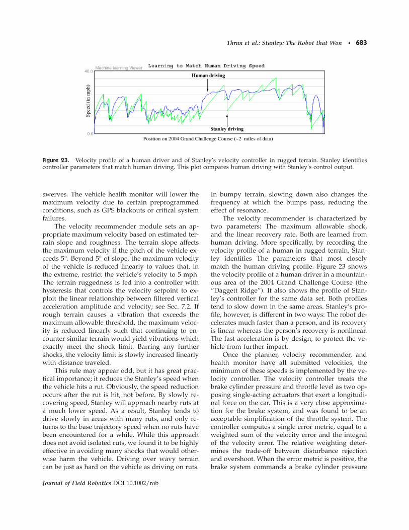
The velocity recommender is characterized bytwo parameters: The maximum allowable shock,and the linear recovery rate. Both are learned fromhuman driving. More specifically, by recording thevelocity profile of a human in rugged terrain, Stan-ley identifies The parameters that most closelymatch the human driving profile. Figure 23 showsthe velocity profile of a human driver in a mountain-ous area of the 2004 Grand Challenge Course �the“Daggett Ridge”�. It also shows the profile of Stan-ley’s controller for the same data set. Both profilestend to slow down in the same areas. Stanley’s pro-file, however, is different in two ways: The robot de-celerates much faster than a person, and its recoveryis linear whereas the person’s recovery is nonlinear.The fast acceleration is by design, to protect the ve-hicle from further impact.

Once the planner, velocity recommender, andhealth monitor have all submitted velocities, theminimum of these speeds is implemented by the ve-locity controller. The velocity controller treats thebrake cylinder pressure and throttle level as two op-posing single-acting actuators that exert a longitudi-nal force on the car. This is a very close approxima-tion for the brake system, and was found to be anacceptable simplification of the throttle system. Thecontroller computes a single error metric, equal to aweighted sum of the velocity error and the integralof the velocity error. The relative weighting deter-mines the trade-off between disturbance rejectionand overshoot. When the error metric is positive, thebrake system commands a brake cylinder pressure

Figure 23. Velocity profile of a human driver and of Stanley’s velocity controller in rugged terrain. Stanley identifiescontroller parameters that match human driving. This plot compares human driving with Stanley’s control output.



proportional to the PI error metric; and when it isnegative, the throttle level is set proportional to thenegative of the PI error metric. By using the same PIerror metric for both actuators, the system is able toavoid the chatter and dead bands associated withopposing single-acting actuators. To realize the com-manded brake pressure, the hysteretic brake actua-tor is controlled through saturated proportionalfeedback on the brake pressure, as measured by theTouareg, and reported through the CAN businterface.

9.2. Steering Control

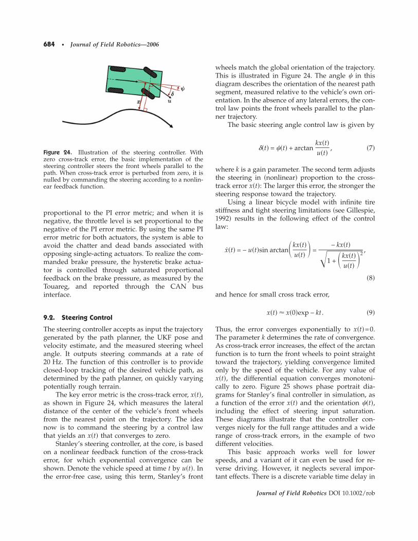
The steering controller accepts as input the trajectorygenerated by the path planner, the UKF pose andvelocity estimate, and the measured steering wheelangle. It outputs steering commands at a rate of20 Hz. The function of this controller is to provideclosed-loop tracking of the desired vehicle path, asdetermined by the path planner, on quickly varyingpotentially rough terrain.

The key error metric is the cross-track error, x�t�,as shown in Figure 24, which measures the lateraldistance of the center of the vehicle’s front wheelsfrom the nearest point on the trajectory. The ideanow is to command the steering by a control lawthat yields an x�t� that converges to zero.

Stanley’s steering controller, at the core, is basedon a nonlinear feedback function of the cross-trackerror, for which exponential convergence can beshown. Denote the vehicle speed at time t by u�t�. Inthe error-free case, using this term, Stanley’s front

wheels match the global orientation of the trajectory.This is illustrated in Figure 24. The angle in thisdiagram describes the orientation of the nearest pathsegment, measured relative to the vehicle’s own ori-entation. In the absence of any lateral errors, the con-trol law points the front wheels parallel to the plan-ner trajectory.

The basic steering angle control law is given by

��t� = �t� + arctankx�t�u�t�

, �7�

where k is a gain parameter. The second term adjuststhe steering in �nonlinear� proportion to the cross-track error x�t�: The larger this error, the stronger thesteering response toward the trajectory.

Using a linear bicycle model with infinite tirestiffness and tight steering limitations �see Gillespie,1992� results in the following effect of the controllaw:

x�t� = − u�t�sin arctan� kx�t�u�t� � =

− kx�t�

1 + � kx�t�u�t� �

2,

�8�

and hence for small cross track error,

x�t� x�0�exp − kt . �9�

Thus, the error converges exponentially to x�t�=0.The parameter k determines the rate of convergence.As cross-track error increases, the effect of the arctanfunction is to turn the front wheels to point straighttoward the trajectory, yielding convergence limitedonly by the speed of the vehicle. For any value ofx�t�, the differential equation converges monotoni-cally to zero. Figure 25 shows phase portrait dia-grams for Stanley’s final controller in simulation, asa function of the error x�t� and the orientation �t�,including the effect of steering input saturation.These diagrams illustrate that the controller con-verges nicely for the full range attitudes and a widerange of cross-track errors, in the example of twodifferent velocities.

This basic approach works well for lowerspeeds, and a variant of it can even be used for re-verse driving. However, it neglects several impor-tant effects. There is a discrete variable time delay in

Figure 24. Illustration of the steering controller. Withzero cross-track error, the basic implementation of thesteering controller steers the front wheels parallel to thepath. When cross-track error is perturbed from zero, it isnulled by commanding the steering according to a nonlin-ear feedback function.



the control loop, inertia in the steering column, andmore energy to dissipate as speed increases. Theseeffects are handled by simply damping the differ-ence between steering command and the measuredsteering wheel angle, including a term for yawdamping. Finally, to compensate for the slip of theactual pneumatic tires, the vehicle is commanded tohave a steady-state yaw offset that is a nonlinearfunction of the path curvature and the vehicle speed,based on a bicycle vehicle model, with slip, that wascalibrated and verified in testing. These terms com-bine to stabilize the vehicle and drive the cross-trackerror to zero, when run on the physical vehicle. Theresulting controller has proven stable in testing onterrain from pavement to deep off-road mudpuddles, and on trajectories with tight enough radiiof curvature to cause substantial slip. It typicallydemonstrates tracking error that is on the order ofthe estimation error of this system.

10. DEVELOPMENT PROCESS AND RACERESULTS

10.1. Race Preparation

The race preparation took place at three different lo-cations: Stanford University, the 2004 Grand Chal-lenge Course between Barstow and Primm, and the

Sonoran Desert near Phoenix, AZ. In the weeks lead-ing up to the race, the team permanently moved toArizona, where it enjoyed the hospitality of Volk-swagen of America’s Arizona Proving Grounds. Fig-ure 26 shows examples of hardware testing in ex-treme offroad terrain; these pictures were takenwhile the vehicle was operated by a person.

In developing Stanley, the Stanford Racing Teamadhered to a tight development and testing sched-ule, with clear milestones along the way. Emphasiswas placed on early integration, so that an end-to-end prototype was available nearly a year before therace. The system was tested periodically in desertenvironments representative of the team’s expecta-tion for the Grand Challenge race. In the monthsleading up to the race, all software and hardwaremodules were debugged and subsequently frozen.The development of the system terminated wellahead of the race.

The primary measure of system capability was“MDBCF”—mean distance between catastrophicfailures. A catastrophic failure was defined as a con-dition under which a human driver had to inter-vene. Common failures involved software problems,such as the one shown in Figure 9; occasional fail-ures were caused by the hardware, e.g., the vehiclepower system. In December 2004, the MDBCF wasapproximately 1 mile. It increased to 20 miles in July2005. The last 418 miles before the National Qualifi-cation Event were free of failures; this included a

Figure 25. Phase portrait for k=1 at 10 and 40 m per second, respectively, for the basic controller, including the effect ofsteering input saturation.



single 200-mile run over a cyclic testing course. Atthat time, the system development was suspended,Stanley’s lateral navigation accuracy was approxi-mately 30 cm. The vehicle had logged more than1,200 autonomous miles.

In preparing for this race, the team also testedsensors that were not deployed in the final race.Among them was an industrial strength stereo vi-sion sensor with a 33 cm baseline. In early experi-ments, we found that the stereo system provided ex-cellent results in the short range, but lagged behindthe laser system in accuracy. The decision not to usestereo was simply based on the observation that itadded little to the laser system. A larger baselinemight have made the stereo more useful at longerranges, but was unfortunately not available.

The second sensor that was not used in the racewas the 24 GHz RADAR system. The RADAR uses alinear frequency shift keying modulated �LFMSK�transmit wave form; it is normally used for adaptivecruise control. After carefully tuning gains and ac-ceptance thresholds of the sensor, the RADARproved highly effective in detecting large frontal ob-stacles such as abandoned vehicles in desert terrain.Similar to the monovision system in Sec. 6, the RA-DAR was tasked to screen the road at a range be-yond the laser sensors. If a potential obstacle wasdetected, the system limits Stanley’s speed to25 mph so that the lasers could detect the obstacle intime for collision avoidance.

While the RADAR system proved highly effec-tive in testing, two reasons prevented its use in therace. The first reason was technical: During theNQE, the USB driver of the receiving computer re-peatedly caused trouble, sometimes stalling the re-ceiving computer. The second reason was pragmati-cal. During the NQE, it became apparent that theprobability of encountering large frontal obstacleswas small in high-speed zones; and even if thoseexisted, the vision system would very likely detect

them. As a consequence, the team felt that the tech-nical risks associated with the RADAR system out-weighed its benefits, and made the decision not touse RADAR in the race.

Figure 26. Vehicle testing at the Volkswagen Arizona Proving Grounds, manual driving.

Figure 27. This map shows Stanley’s path. The thicknessof the trajectory indicates Stanley’s speed �thicker meansfaster�. At the locations marked by the red “x”s, the raceorganizers paused Stanley because of the close proximityof CMU’s H1ghlander robot. At Mile 101.5, H1ghlanderwas paused and Stanley passed. This location is markedby a green “x”.



10.2. National Qualification Event

The NQE took place from September 27 to October 5on the California Speedway in Fontana, CA. Likemost competitive robots, Stanley qualified after fourtest runs. From the 43 semifinalists, 11 completed the

course in the first run, 13 in the second run, 18 in thethird run, and 21 in the fourth run. Stanley’s timeswere competitive, but not the fastest �Run 1—10:38;Run 2—9:12; Run 3—11:06; and Run 4—11:06�. How-ever, Stanley was the only vehicle that cleared all 50

Figure 28. Passing CMU’s H1ghlander robot: The left column shows a sequence of camera images, the center column theprocessed images with obstacle information overlayed; and the right column, the 2D map derived from the processedimage. The vision routine detects H1ghlander as an obstacle at a 40 m range, approximately twice the range of the lasers.



gates in every run, and avoided collisions with all ofthe obstacles. This flawless performance earnedStanley the number two starting position, behindCMU’s H1ghlander robot and ahead of the slightlyfaster Sandstorm robot, also by CMU.

10.3. The Race

At approximately 4:10 am on October 8, 2005, theStanford Racing Team received the race data, whichconsisted of 2,935 GPS-referenced coordinates, alongwith speed limits of up to 50 mph. Stanley startedthe race at 6:35 am on October 8, 2005. The robotimmediately picked up speed and drove at or justbelow the speed limit. 3 h, 45 min, and 22 s into therace, at Mile 73.5, DARPA paused Stanley for thefirst time, to give more space to CMU’s H1ghlanderrobot, which had started five minutes ahead of Stan-ley. The first pause lasted 2 min 45 s. Stanley waspaused again only 5 min 40 s later, at Mile 74.9 �3 h,53 min, and 47 s into the race�. This time the pauselasted 6 min 35 s, for a total pause time of 9 min20 s. The locations of the pauses are shown in Figure27. From this point on, Stanley repeatedly ap-proached H1ghlander within a few hundred yards.Even though Stanley was still behind H1ghlander, itwas leading the race.

5 h, 24 min, 45 s into the race, DARPA finallypaused H1ghlander and allowed Stanley to pass.The passing happened a Mile 101.5; the location ismarked by a green circle in Figure 27. Figure 28shows processed camera images of the passing pro-cess acquired by Stanley, and Figure 29 depicts a 3Dmodel of H1ghlander as it is being passed. SinceStanley started in second pole position and finished

first, the top-seeded H1ghlander robot was the onlyrobot encountered by Stanley during the race.

As noted in the Introduction of this paper, Stan-ley finished first, at an unmatched finishing time of6 h, 53 min, and 58 s. Its overall average velocitywas 19.1 mph. However, Stanley’s velocity variedwildly during the race. Initially, the terrain was flatand the speed limits allowed for much higherspeeds. Stanley reached its top speed of 38.0 mph atMile 5.43, 13 min and 47 s into the race. Its maxi-mum average velocity during the race was 24.8 mph,which Stanley attained after 16 min and 56 s, at Mile7.00. Speed limits then forced Stanley to slow down.Between Mile 84.9 and 88.1, DARPA restricted themaximum velocity to 10 mph. Shortly thereafter, atMile 90.6 and 4 h, 57 min, and 7 s into the race, Stan-ley attained its minimum average velocity of18.3 mph. The total profile of velocities is shown inFigure 30.

As explained in this paper, Stanley uses a num-ber of strategies to determine the actual travel speed.During 68.2% of the course, Stanley’s velocity waslimited as precalculated, by following the DARPAspeed limits or the maximum lateral accelerationconstraints in turns. For the remaining 31.8%, Stan-ley chose to slow down dynamically, as the result ofits sensor measurements. In 18.1%, the slow downwas the result of rugged or steep terrain. The visionmodule caused Stanley to slow down to 25 mph for13.1% of the total distance; however, without the vi-sion module Stanley would have been forced to a25 mph maximum speed, which would have re-sulted in a finishing time of approximately 7 h and5 min, possibly behind CMU’s Sandstorm robot. Fi-nally, for 0.6% of the course, Stanley drove slowerbecause it was denied GPS readings. Figure 31 illus-trates the effect of terrain ruggedness on the overallvelocity. The curve on the top illustrates the magni-tude at which Stanley slowed down to accommodaterugged terrain; the bottom diagram shows the alti-tude profile, as provided by DARPA. The terrainruggedness triggers mostly in mountainous terrain.We believe that the ability to adapt the speed to theruggedness of the terrain was an essential ingredientin Stanley’s success.

Stanley also encountered some unexpected diffi-culties along the course. Early on in the race, Stan-ley’s laser data stream repeatedly stalled for dura-tions of 300 to 1,100 ms. There were a total of 17incidents, nearly all of which occurred between Mile22 and Mile 35. The resulting inaccurate time stamp-

Figure 29. Laser model of CMU’s H1ghlander robot,taken at Mile 101.5.



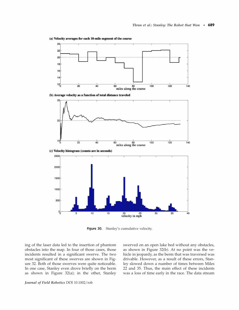
ing of the laser data led to the insertion of phantomobstacles into the map. In four of those cases, thoseincidents resulted in a significant swerve. The twomost significant of these swerves are shown in Fig-ure 32. Both of those swerves were quite noticeable.In one case, Stanley even drove briefly on the bermas shown in Figure 32�a�; in the other, Stanley

swerved on an open lake bed without any obstacles,as shown in Figure 32�b�. At no point was the ve-hicle in jeopardy, as the berm that was traversed wasdrivable. However, as a result of these errors, Stan-ley slowed down a number of times between Miles22 and 35. Thus, the main effect of these incidentswas a loss of time early in the race. The data stream

Figure 30. Stanley’s cumulative velocity.



stalling problem vanished entirely after Mile 37.85. Itonly reoccurred once at Mile 120.66, without any vis-ible change of the driving behavior.

During 4.7% of the Grand Challenge, the GPSreported 60 cm error or more. Naturally, this num-ber represents the unit’s own estimate, which maynot necessarily be accurate. However, this raises thequestion of how important online mapping and pathplanning was in this race.

Stanley frequently moved away from the centeraxis of the RDDF. On average, the lateral offset was±74 cm. The maximum lateral offset during the racewas 10.7 m, which was the result of the swerveshown in Figure 32�c�. However, such incidents wererare, and in nearly all cases nonzero lateral offsetswere the results of obstacles in the robot’s path.

An example situation is depicted in Figure 33.This figure shows raw laser data from the BeerBottle Pass, the most difficult section of the course.An image of this pass is depicted in Figure 34�a�. Of

interest is the map in Figure 34�b�. Here the DARPA-provided corridor is marked by the two solid bluelines. This image illustrates that the berm on Stan-ley’s left reaches well into the corridor. Stanleydrives as far left as the corridor constraint allows.Figure 35 shows a histogram of lateral offsets for theBeer Bottle Pass. On average, Stanley drove 66 cm tothe right of the center of the RDDF in this part of the

Figure 31. This diagram shows where the road condi-tions forced Stanley to slow down along the race course.Slow down predominately occurred in the mountains.

Figure 32. Problems during the race caused by a stalling of the laser data stream. In both cases, Stanley swerved aroundphantom obstacles; at Mile 22.37 Stanley drove on the berm. None of these incidents led to a collision or an unsafe drivingsituation during the race.

Figure 33. Sensor image from the Beer Bottle Pass, themost difficult passage of the DARPA Grand Challenge.



race. We suspect that driving 66 cm further to theleft would have been fatal in many places. Thissheds light on the importance of Stanley’s ability toreact to the environment in driving. Simply follow-ing the GPS points would likely have preventedStanley from finishing this race.

11. DISCUSSION

This paper provides a comprehensive survey of thewinning robot of the DARPA Grand Challenge. Stan-ley, developed by the Stanford Racing Team in col-laboration with its primary supporters, relied on asoftware pipeline for processing sensor data and de-termining suitable steering, throttle, brake, and gearshifting commands.

From a broad perspective, Stanley’s software mir-rors common methodology in autonomous vehiclecontrol. However, many of the individual modulesrelied on state-of-the-art artificial intelligence tech-niques. The pervasive use of machine learning, bothahead and during the race, made Stanley robust and

precise. We believe that those techniques, along withthe extensive testing that took place, contributed sig-nificantly to Stanley’s success in this race.

While the DARPA Grand Challenge was a mile-stone in the quest for self-driving cars, it left open anumber of important problems. Most importantamong those was the fact that the race environmentwas static. Stanley is unable to navigate in traffic. Forautonomous cars to succeed, robots, such as Stanley,must be able to perceive and interact with movingtraffic. While a number of systems have shown im-pressive results �Dickmanns et al., 1994; Hebert,Thorpe & Stentz, 1997; Pomerleau & Jochem, 1996�,further research is needed to achieve the level of re-liability necessary for this demanding task. Evenwithin the domain of driving in static environments,Stanley’s software can only handle limited types ofobstacles. For example, the present software wouldbe unable to distinguish tall grass from rocks, a re-search topic that has become highly popular in recentyears �Dima & Hebert, 2005; Happold, Ollis &Johnson, 2006; Wellington, Courville & Stentz, 2005�.

ACKNOWLEDGMENTS

The Stanford Racing Team �SRT� was sponsored byfour Primary Supporters: Volkswagen of America’sElectronics Research Lab, Mohr Davidow Ventures,Android, and Red Bull. The Primary Supporters, to-gether with the Stanford team leaders, formed theSRT Steering Committee, which oversaw the SRT op-erations. The SRT also received support from Intel

Figure 34. Image of the Beer Bottle pass, and snapshot of the map acquired by the robot. The two blue contours in themap mark the GPS corridor provided by DARPA, which aligns poorly with the map data. This analysis suggests that arobot that followed the GPS via points blindly would likely have failed to traverse this narrow mountain pass.

Figure 35. Histogram of lateral offsets on the beer bottlepass. The horizontal units are in centimeters.



Research, Honeywell, Tyzx, Inc., and Coverity, Inc.Generous financial contributions were made byDavid Cheriton, the Johnson Family, and Vint Cerf.A huge number of individuals at Stanford, Volk-swagen, and related facilities helped us in develop-ing this robot, which is gratefully acknowledged.

The SRT also thanks DARPA for organizing thisgreat race and the many journalists who providedpress coverage. Our final gratitude goes to the manyfriends we made preparing for and during the event,and the many people who helped us and otherteams along the way.

REFERENCES

Brooks, C., & Iagnemma, K. �2005�. Vibration-based terrainclassification for planetary exploration rovers. IEEETransactions on Robotics, 21�6�, 185–1191.

Crisman, J., & Thorpe, C. �1993�. SCARF: A color visionsystem that tracks roads and intersections. IEEETransactions on Robotics and Automation, 9�1�, 49–58.

DARPA. �2004�. DARPA Grand Challenge rulebook. Re-trieved from http://www.darpa.mil/grandchallenge05/Rules_8oct04.pdf.

Davies, B., & Lienhart, R. �2006�. Using CART to segmentroad images. In Proceedings SPIE Multimedia Con-tent Analysis, Management, and Retrieval, San Jose,CA.

Dickmanns, E. �2002�. Vision for ground vehicles: Historyand prospects. International Journal of Vehicle Au-tonomous Systems, 1�1�, 1–44.

Dickmanns, E., Behringer, R., Dickmanns, D., Hildebrandt,T., Maurer, M., Schiehlen, J., & Thomanek, F. �1994�.The seeing passenger car VaMoRs-P. In Proceedingsof the International Symposium on Intelligent Ve-hicles, Paris, France.

Dima, C., & Hebert, M. �2005�. Active learning for outdoorobstacle detection. In S. Thrun, G. Sukhatme, S.Schaal, & O. Brock �Eds.�, Proceedings of the RoboticsScience and Systems Conference, Cambridge, MA.Cambridge, MA: MIT Press.

Duda, R., & Hart, P. �1973�. Pattern classification and sceneanalysis. New York: Wiley.

Ettinger, S., Nechyba, M., Ifju, P., & Waszak, M. �2003�.Vision-guided flight stability and control for microairvehicles. Advanced Robotics, 17, 617–640.

Farrell, J., & Barth, M. �1999�. The global positioning sys-tem. New York: McGraw-Hill.

Gat, E. �1998�. Three-layered architectures. In D. Korten-kamp, R. Bonasso, & R. Murphy �Eds.�, AI-based mo-bile robots: Case studies of successful robot systems�pp. 195–210�. Cambridge, MA: MIT Press.

Gillespie, T. �1992�. Fundamentals of vehicle dynamics.Warrendale, PA: SAE Publications.

Happold, M., Ollis, M., & Johnson, N. �2006�. Enhancingsupervised terrain classification with predictive unsu-pervised learning. In G. Sukhatme, S. Schaal, W. Bur-gard, & D. Fox �Eds.�, Proceedings of the Robotics Sci-ence and Systems Conference, Philadelphia, PA.Cambridge, MA: MIT Press.

Hebert, M., Thorpe, C., & Stentz, A. �1997�. Intelligent un-manned ground vehicles: Autonomous navigation re-search at Carnegie Mellon University. Dordrecht: Klu-wer Academic.

Iagnemma, K., & Dubowsky, S. �2004�. Mobile robots inrough terrain: Estimation, motion planning, and con-trol with application to planetary rovers. SpringerTracts in Advanced Robotics �STAR� Series. Berlin:Springer.

Julier, S., & Uhlmann, J. �1997�. A new extension of theKalman filter to nonlinear systems. In InternationalSymposium on Aerospace/Defense Sensing, Simulateand Controls, Orlando, FL.

Kelly, A., & Stentz, A. �1998�. Rough terrain autonomousmobility, part 1: A theoretical analysis of require-ments. Autonomous Robots, 5, 129–161.

Ko, N., & Simmons, R. �1998�. The lane-curvature methodfor local obstacle avoidance. In Proceedings of theIEEE/RSJ International Conference on Intelligent Ro-bots and Systems �IROS�, Victoria, Canada. New York:IEEE Industrial Electronics Society.

Pomerleau, D.A. �1991�. Rapidly adapting neural networksfor autonomous navigation. In R.P. Lippmann, J.E.Moody, & D.S. Touretzky �Eds.�, Advances in neuralinformation processing systems 3 �pp. 429–435�. SanMateo: Morgan Kaufmann.

Pomerleau, D.A. �1993�. Knowledge-based training of arti-ficial neural networks for autonomous robot driving.In J.H. Connell & S. Mahadevan �Eds.�, Robot learning�pp. 19–43�. New York: Kluwer Academic.

Pomerleau, D., & Jochem, T. �1996�. Rapidly adapting ma-chine vision for automated vehicle steering. IEEE Ex-pert, 11�2�, 19–27.

Simmons, R., & Apfelbaum, D. �1998�. A task descriptionlanguage for robot control. In Proceedings of the Con-ference on Intelligent Robots and Systems �IROS�, Vic-toria, CA. New York: IEEE Industrial ElectronicsSociety.

van der Merwe, R. �2004�. Sigma-point Kalman filters forprobabilistic inference in dynamic state-space models.Unpublished Ph.D. thesis, Oregon Graduate InstituteSchool of Science and Engineering, Beaverton,Oregon.

van der Merwe, R., & Wan, E. �2004�. Sigma-point Kalmanfilters for integrated navigation. In Proceedings of the60th Annual Meeting of The Institute of Navigation�ION�, Dayton, OH.

Wellington, C., Courville, A., & Stentz, A. �2005�. Interact-ing Markov random fields for simultaneous terrainmodeling and obstacle detection. In S. Thrun, G.Sukhatme, S. Schaal & O. Brock �Eds.�, Proceedings ofthe Robotics Science and Systems Conference, Cam-bridge, MA. Cambridge, MA: MIT Press.



Documents

Stanley: The robot that won the DARPA Grand Challengerobots.stanford.edu/papers/thrun.stanley05.pdf · 3000 Sand Hill Road, Bldg. 3, Suite 290 ... which won the 2005 DARPA Grand Challenge