SCHEDULING IISCHEDULING II Giovanni DeGiovanni De Micheli Micheli

Stanford UniversityStanford University

Scheduling under resourceScheduling under resourceconstraintsconstraints

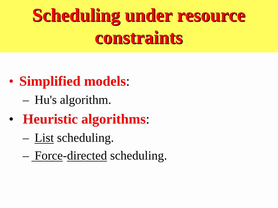
• Simplified models:– Hu's algorithm.

• Heuristic algorithms:– List scheduling.– Force-directed scheduling.

Hu'sHu's algorithm algorithm

• Assumptions:– Graph is a forest.– All operations have unit delay.– All operations have the same type.

• Algorithm:– Label vertices with distance from sink.– Greedy strategy.– Exact solution.

Example of using Example of using Hu’s Hu’s algorithmalgorithm

• Assumptions:– One resource type only.– All operations have unit delay.

AlgorithmAlgorithmHu'sHu's schedule with schedule with aa resources resources

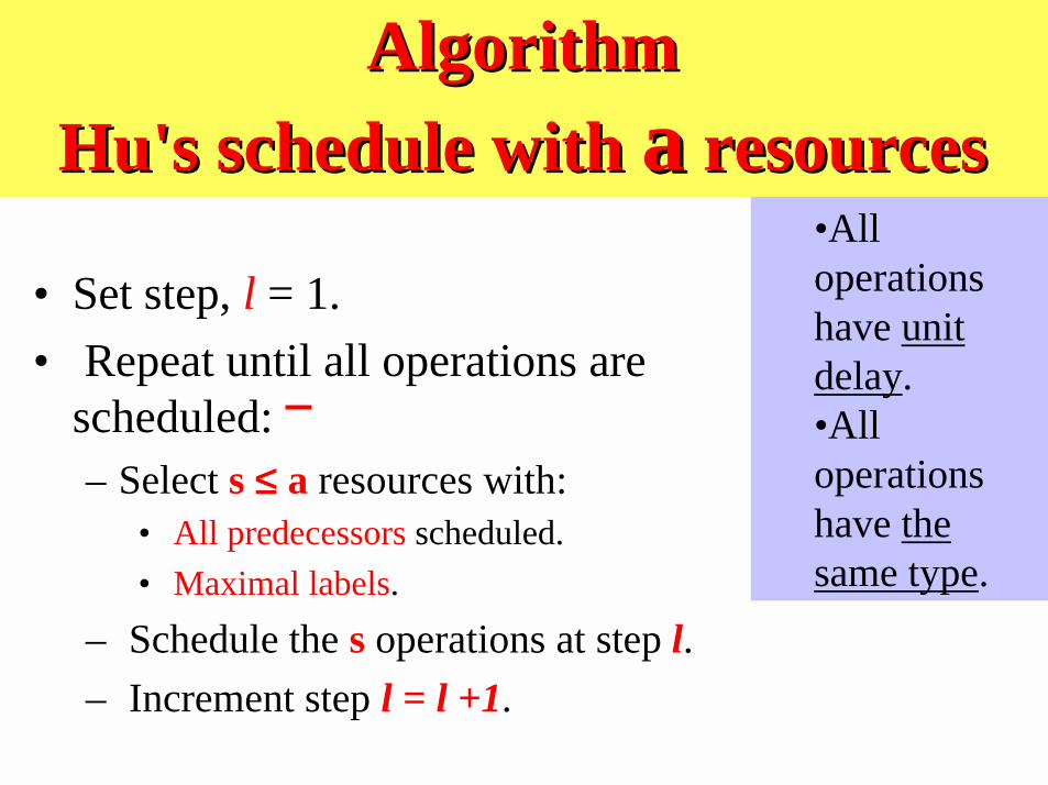
• Set step, l = 1.• Repeat until all operations are

scheduled:– Select s ≤≤≤≤ a resources with:

• All predecessors scheduled.• Maximal labels.

– Schedule the s operations at step l.– Increment step l = l +1.

•Alloperationshave unitdelay.•Alloperationshave thesame type.

• Minimum latency with a= 3 resources.– Step 1:

• Select {v 1 , v 2 , v 6 }.

– Step 2:• Select {v 3 , v 7 , v 8 }.

– Step 3:• Select {v 4 , v 9 , v 10 }.

– Step 4:• Select {v 5 , v 11 }.

AlgorithmAlgorithmHu'sHu's schedule with schedule with aa resources resources

We always select3 resources

Exactness ofExactness of Hu's Hu's algorithm algorithm• Theorem1:

– Given a DAG with operations of the same type.

• a is a lower bound on the number of resources to complete aschedule with latency λλλλλλλλ .•• γγγγγγγγ is a positive integer.• Theorem2:

•Hu's algorithm applied to a tree with unit-cycle resourcesachieves latency λλλλλλλλ with a resources.

• Corollary:• Since a is a lower bound on the number of resources forachieving λλλλλλλλ, then λλλλλλλλ is minimum.

List schedulingList scheduling algorithms algorithms

• Heuristic method for:– 1. Minimum latency subject to resource bound.

– 2. Minimum resource subject to latency bound.

• Greedy strategy (like Hu's).• General graphs (unlike Hu's).• Priority list heuristics.

– Longest path to sink.– Longest path to timing constraint.

1. List scheduling algorithm1. List scheduling algorithmfor minimum latency for resource boundfor minimum latency for resource bound

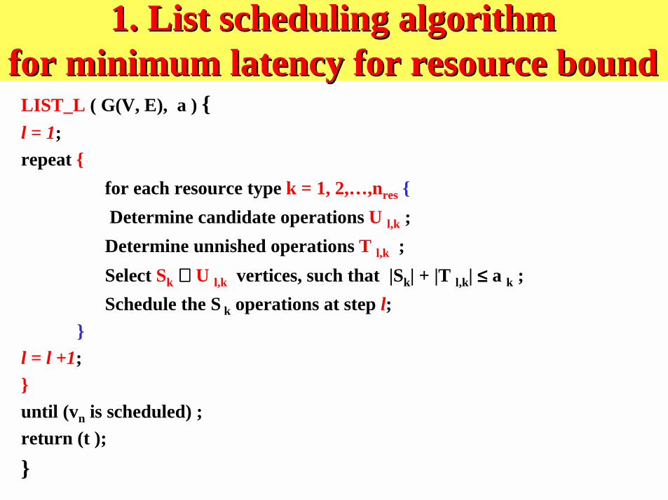
LIST_L ( G(V, E), a ) {l = 1;repeat { for each resource type k = 1, 2,…,nres { Determine candidate operations U l,k ; Determine unnished operations T l,k ; Select Sk ⊆⊆⊆⊆ U l,k vertices, such that |Sk| + |T l,k| ≤≤≤≤ a k ; Schedule the S k operations at step l; }l = l +1;}until (vn is scheduled) ;return (t );

}

• Assumptions:– a 1 = 3 multipliers

with delay 2.– a 2 = 1 ALUs with

delay 1.

List scheduling algorithmList scheduling algorithmfor minimum latencyfor minimum latency

1. List scheduling algorithm1. List scheduling algorithmfor minimum latency for resource boundfor minimum latency for resource bound

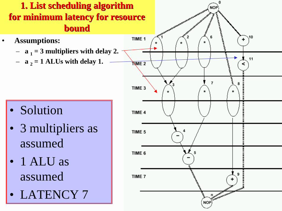
• Solution• 3 multipliers as

assumed• 1 ALU as

assumed• LATENCY 7

• Assumptions:– a 1 = 3 multipliers with delay 2.– a 2 = 1 ALUs with delay 1.

1. List scheduling algorithm1. List scheduling algorithmfor minimum latency for resourcefor minimum latency for resource

boundbound

2.2. List scheduling algorithm for minimum resource usage List scheduling algorithm for minimum resource usage

LIST_R ( G(V,E), λλλλ ) { aa = 1 ; Compute the latest possible start times tL by ALAP ( G(V,E), λλλλ); if ( t L 0 < 0 ) return (φφφφ); l = 1; repeat {{ for each resource type k = 1,2,…, nres {{ Determine candidate operations U l k ; Compute the slacks

Schedule the candidate operations with zero slack and update aa ; Schedule the candidate operations that do not require additional resources; }} l = l +1; }}until (vn is scheduled) ;return (t, a );}

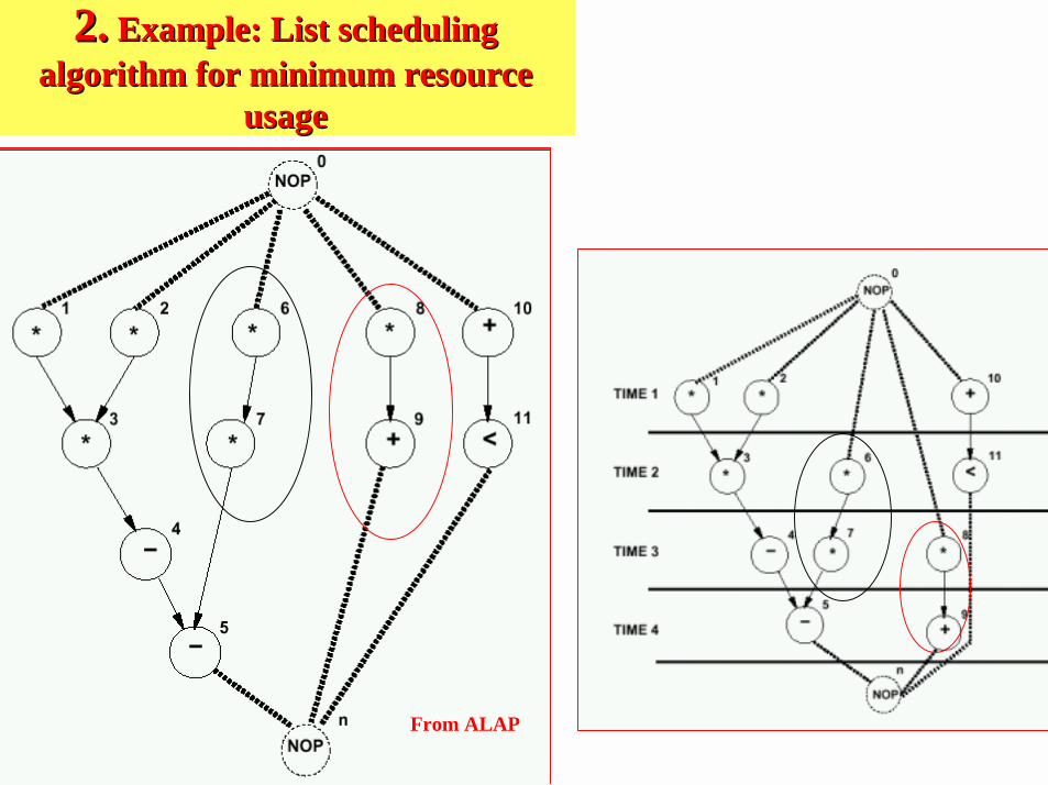
2.2. Example: List scheduling Example: List schedulingalgorithm for minimum resourcealgorithm for minimum resource

usageusage

From ALAP

FForce-orce-ddirected schedulingirected scheduling• Heuristic scheduling methods [Paulin]:

– 1. Minimum latency subject to resource bound.• Variation of list sscheduling: FDLS.

– 2. Minimum resource subject to latency bound.• Schedule one operation at a time.

• Rationale:– Reward uniform distribution of operations across

schedule steps.

Force-directed scheduling Force-directed scheduling definitionsdefinitions

• Operation interval: mobility plus one (µµµµ i+1).– Computed by ASAP and ALAP scheduling

[t S i , t L i ].• Operation probability p i (l) :

– Probability of executing in a given step.– 1/ (µµµµ i +1) inside interval; 0 elsewhere.

• Operation-type distribution q k (l) :– Sum of the operation probabilities for each type.

• Distribution graphs formultiplier and ALU.

Example of Force-directed schedulingExample of Force-directed scheduling

ForceForce• Used as priority function.• Force is related to concurrency.

– Sort operations for least force.• Mechanical analogy:

– Force = constant * displacement.• constant = operation-type

distribution.• displacement = change in

probability.

Example of Force-directed schedulingExample of Force-directed scheduling

Forces related to the assignmentForces related to the assignmentof an operation to a control stepof an operation to a control step

• Self-force:– Sum of forces to other steps.– Self-force for operation v i in step l

• Successor-force:• Related to the successors.• Delaying an operation implies delaying its successors.

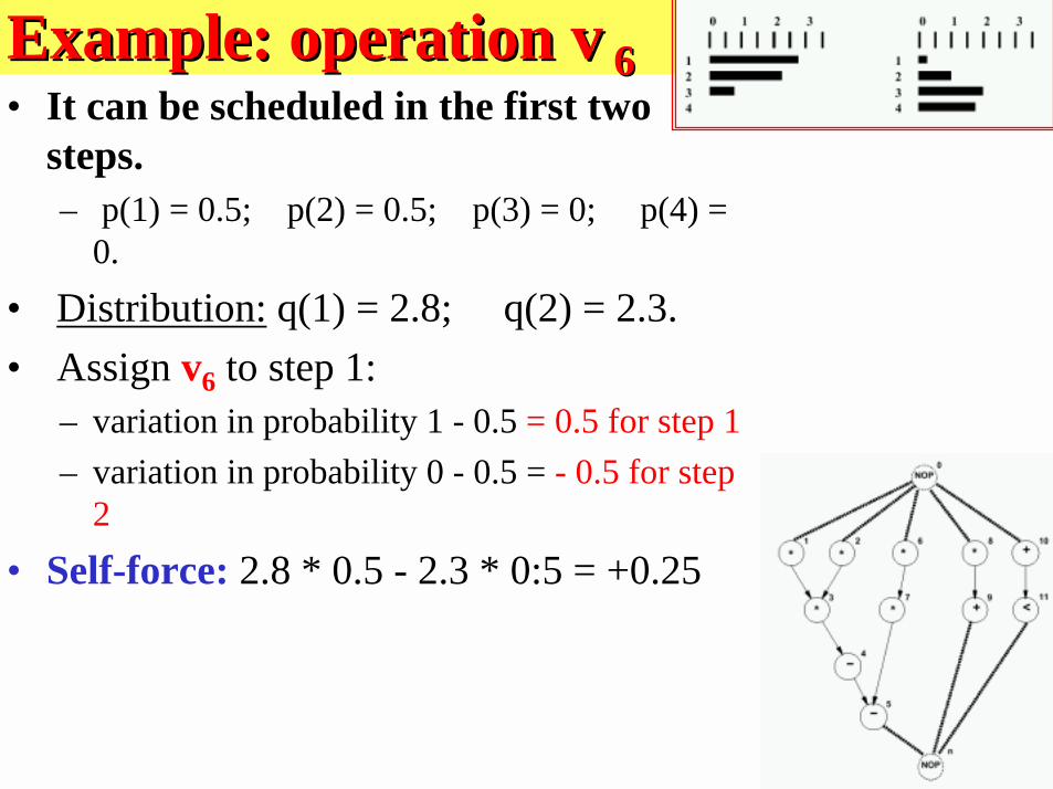
Example: operation vExample: operation v 6 6• It can be scheduled in the first two

steps.– p(1) = 0.5; p(2) = 0.5; p(3) = 0; p(4) =

0.

• Distribution: q(1) = 2.8; q(2) = 2.3.• Assign v6 to step 1:

– variation in probability 1 - 0.5 = 0.5 for step 1– variation in probability 0 - 0.5 = - 0.5 for step

2

• Self-force: 2.8 * 0.5 - 2.3 * 0:5 = +0.25

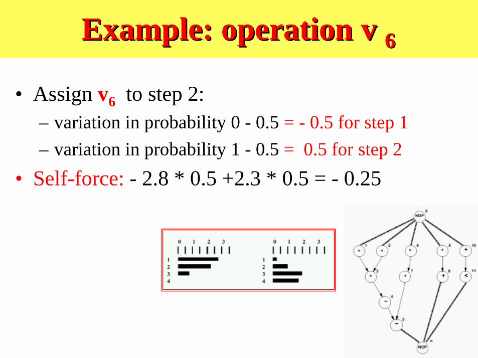
Example: operation v Example: operation v 66

• Assign v6 to step 2:– variation in probability 0 - 0.5 = - 0.5 for step 1– variation in probability 1 - 0.5 = 0.5 for step 2

• Self-force: - 2.8 * 0.5 +2.3 * 0.5 = - 0.25

Example: operation vExample: operation v 6 6

• Successor-force:– Operation v 7 assigned to step 3.– 2.3 (0-0.5) + 0.8 ( 1 -0.5) = - 0.75

• Total-force = -1.• Conclusion:

– Least force is for step 2.– Assigning v 6 to step 2 reduces concurrency.

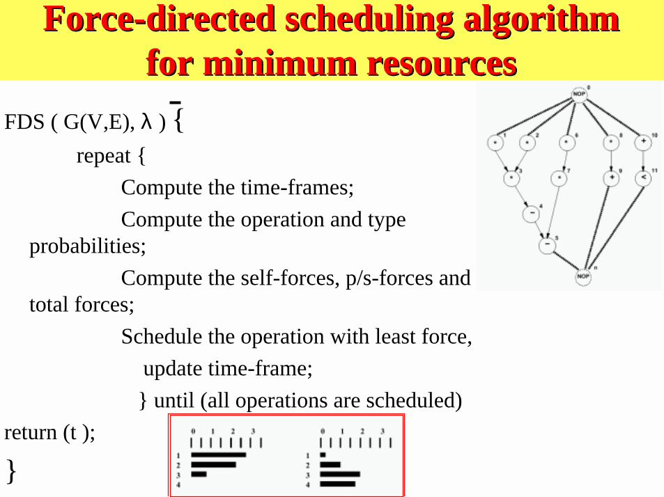
Force-directed scheduling algorithmForce-directed scheduling algorithmfor minimum resourcesfor minimum resources

FDS ( G(V,E), λ ) { repeat { Compute the time-frames; Compute the operation and type

probabilities; Compute the self-forces, p/s-forces and

total forces; Schedule the operation with least force, update time-frame; } until (all operations are scheduled)return (t );

}

Scheduling with chainingScheduling with chaining• Consider propagation delays of resources not in

terms of cycles.• Use scheduling to chain multiple operations in the

same control step.• Useful technique to explore effect of cycle-time on

area/latency trade-off.• Algorithms:

– ILP,– ALAP/ASAP,– List scheduling.

Example of Scheduling with chainingExample of Scheduling with chaining

• Cycle-time: 60.

SummarySummary

• Scheduling determines area/latency trade-off.• Intractable problem in general:

– Heuristic algorithms.– ILP formulation (small-case problems).

• Chaining:– Incorporate cycle-time considerations.