1

Standardized Precipitation Evapotranspiration Index (SPEI) revisited: parameter fitting, evapotranspiration models, tools, datasets and drought monitoring

Santiago Beguería1, Sergio M. Vicente-Serrano2,*, Fergus Reig2, Borja Latorre1

1Estación Experimental de Aula Dei, Consejo Superior de Investigaciones Científicas (EEAD-CSIC), Zaragoza, Spain

2Instituto Pirenaico de Ecología, Consejo Superior de Investigaciones Científicas (IPE-CSIC), Campus de Aula Dei, P.O. Box 13034, E-50059, Zaragoza, Spain

* Corresponding author: svicen@ipe.csic.es

Abstract. The Standardized Precipitation Evapotranspiration Index (SPEI) was developed in 2010 and has been used in an increasing number of climatology and hydrology studies. The objective of this article is to describe computing options that provide flexible and robust use of the SPEI. In particular, we present methods for estimating the parameters of the log-logistic distribution for obtaining standardized values, methods for computing reference evapotranspiration (ET0), and weighting kernels used for calculation of the SPEI at different time scales. We discuss the use of alternative ET0 and actual evapotranspiration (ETa) methods and different options on the resulting SPEI series by use of observational and global gridded data. The results indicate that the equation used to calculate ET0 can have a significant effect on the SPEI in some regions of the world. Although the original formulation of the SPEI was based on plotting-positions Probability Weighted Moment (PWM), we now recommend use of unbiased PWM for model fitting. Finally, we present new software tools for computation and analysis of SPEI series, an updated global gridded database, and a real-time drought-monitoring system. Keywords: Drought, drought index, global warming, evaporation, Penman-Monteith, Standardized Precipitation Index, SPI, Palmer Drought Severity Index, PDSI. 1. Introduction

The Standardized Precipitation Evapotranspiration Index (SPEI) was first proposed by Vicente-Serrano et al. (2010) as an improved drought index that is especially suited for studies of the effect of global warming on drought severity. Like the Palmer Drought Severity Index (PDSI), the SPEI considers the effect of reference evapotranspiration on drought severity, but the multi-scalar nature of the SPEI enables identification of different drought types and drought impacts on diverse systems (Vicente-Serrano et al., 2012, 2013). Thus, the SPEI has the sensitivity of the PDSI in measurement of evapotranspiration demand (caused by fluctuations and trends in climatic variables other than precipitation), is simple to calculate, and is multi-scalar, like the Standardized Precipitation Index (SPI). Vicente-Serrano et al. (2010, 2010b, 2011, 2012) provided complete descriptions of the theory behind the SPEI, the computational details, and comparisons with other popular drought indicators such as the PDSI (Palmer, 1965) and the SPI (McKee et al., 1993).

The procedure for calculating the SPEI is similar to that for the SPI. However, the SPEI uses “climatic water balance”, the difference between precipitation and reference evapotranspiration (P – ET0), rather than precipitation (P) as the input. The climatic water balance compares the available water (P) with the atmospheric

2

evaporative demand (ET0), and therefore provides a more reliable measure of drought severity than only considering precipitation. The climatic water balance is calculated at various time scales (i.e. over one month, two months, three months, etc.), and the resulting values are fit to a log-logistic probability distribution to transform the original values to standardized units that are comparable in space and time and at different SPEI time scales.

Although the SPEI was only recently developed, it has been used in diverse studies that have analyzed drought variability (Potop, 2011; Paulo et al., 2012; Wei-Guang et al., 2012; Li et al., 2012; Spinoni et al., 2013; Sohn et al., 2013), drought reconstruction (Allen et al., 2011), drought atmospheric mechanisms (Vicente-Serrano et al., 2011b; Boroneant et al., 2011; Seibert, 2012), climate change (Abiodun et al., 2012; Wolf and Abatzoglou, 2011; Soo-Jin et al., 2012, Yu et al., 2013), and identification of drought impacts on hydrological (Lorenzo-Lacruz et al., 2010; McEvoy et al., 2012; Wolf, 2012), agricultural (Potop et al., 2012), and ecological systems (Deng et al., 2011; Toromani et al., 2011; Vicente-Serrano et al., 2010c; Vicente-Serrano, 2012b, 2013a; Drew et al., 2012; Martin, 2012; Levesque et al., 2013; Cavin et al., 2013; Barbeta et al., 2013). In addition, the SPEI has been used in drought monitoring systems (e.g., Fuchs et al., 2012). Several of these studies reported that the SPEI correlated better with hydrological and ecological variables than other drought indices in a variety of natural and managed systems.

Several issues have appeared after extensive use of the SPEI in the past 2 years, and these have led to improved formulations of the SPEI. These improved formulations are related to: (i) the method that parameters of the log-logistic distribution are estimated to obtain SPEI values; (ii) the method used to calculate ET0; and (iii) the weighting kernel used for computation of climatic water balance at time scales larger than one month. In response, we have developed additional improvements: (iv) a set of computing tools for calculation and analysis of the SPEI, (v) an improved global gridded database, and (vi) an operative real-time global drought monitoring system based on the SPEI.

Estimation of the log-logistic parameters is important because spatial and temporal comparability of drought indices is important for accurate drought analysis and monitoring (Nkemdirim and Weber, 1999). For this reason, it is necessary that SPEI series at different sites have the same average (x = 0) and Standard Deviation (SD = 1); the same is applicable to series of the SPEI recorded at the same location but at different time-scales. Parameter estimation can lead to bias and errors in variance, so the method used for estimation is very important. In Section 2 of this article, we identify some problems related to the plotting-positions Probability Weighted Moment (PWM) method used in the original formulation of the SPEI, and suggest use of an unbiased PWM as an alternative.

The use of actual evapotranspiration (ETa) instead of the reference evapotranspiration (ET0) has been suggested in calculating drought indices. Computation of ETa, however, introduces a number of additional problems, and it is not totally clear whether ETa is a good variable to consider when estimating drought. Here we discuss on the use of ETa and ET0 for drought quantification and on particularly on the SPEI calculation.

The original formulation of the SPEI suggested use of the Thornthwaite (Th) equation for estimation of ET0 (Thornthwaite, 1948). This equation only requires mean daily temperature and latitude of the site, and it was used due to limited data availability. However, previous research indicated that the Th equation underestimated

3

ET0 in arid and semiarid regions (Jensen et al., 1990), and overestimated ET0 in humid equatorial and tropical regions (van der Schrier et al., 2011). Moreover, this equation leads to an overestimation of ET0 with increasing air temperature and it does not accurately estimate the evolution of ET0 over the last decades (Donohue et al., 2010).

The use of a particular equation for estimation of ET0 is not central for the calculation of SPEI. Thus, the International Commission for Irrigation (ICID), the Food and Agriculture Organization of the United Nations (FAO), and the American Society of Civil Engineers (ASCE) (Allen et al., 1998; Walter et al., 2000) have used the Penman-Monteith (PM) equation for calculation of ET0. However, the PM equation requires extensive data (solar radiation, temperature, wind speed, and relative humidity), that many meteorological stations do not routinely measure, and long-term records of these variables are not always available. Thus, the Hargreaves (Hg) equation (Hargreaves and Samani, 1985) may be used when this data is not available (Xu and Singh, 2001; Droogers and Allen, 2002). As with the Th equation, the Hg equation has limited data requirements, and only requires daily maximum and minimum temperatures. However, the Hg equation does not have the limitations of the Th equation, and at monthly and annual timescales ET0 estimates from the Hg and PM equations are very similar, with differences less than 2 mm per day (Droogers and Allen, 2002). Hargreaves and Allen (2003) showed that the relationship between monthly ET0 calculated via the Hg equation were within 97% to 101% of that measured by a lysimeter for semi-arid and sub-humid regions of the United States. It is clearly important to test the reliability of the specific ET0 equations that are used for SPEI calculations. Thus, in Section 3 we compared the use of different ET0 equations for calculation of SPEI from observatory and global gridded data.

In subsequent sections of this article, we present new tools and data sources that can be used for computation of the SPEI. In Section 4, we present a software package used to compute the SPEI, which describes the various alternatives presented in this article and other alternatives such as the use of different temporal kernels. In Section 5, we present an improved global gridded dataset of the SPEI. Finally, in Section 6 we present a new real-time global drought monitoring system based on the SPEI.

The main objective of this article is to provide more flexible and robust options for computation and use of the SPEI, explain possible sources of error, and provide advice on the use of the different ET0 equations. 2. Estimation of Log-logistic parameters

We previously showed that the log-logistic distribution provided better results than other distributions for obtaining SPEI series in standardized z units (mean = 0, SD = 1) (Vicente-Serrano et al. 2010). The probability distribution function of a variable D according to a log-logistic distribution is given by:

𝐹 𝐷 = 1+ !!!!

! !!, (eq. 1)

where α, β, and γ represent the scale, shape and location parameters that are estimated from the sample D (difference between Precipitation and ET0). Originally, Hosking (1990) proposed use of Probability Weighted Moments (PWMs) based on the plotting position method. The PWMs of different orders are calculated as:

∑=

−=N

ii

sis DF

Nw

1)1(1

(eq. 2)

4

where ws is the PWM of order s, N is the number of data points, Fi is a frequency estimator, and Di is the difference between Precipitation and Reference Evapotranspiration for month i.

The plotting position method is very easy to implement. Alternative PWM estimators can be obtained by other methods, such as the unbiased estimator (Hosking, 1986):

𝑤! =!!

!!!! !!!!!!

!!!! (eq. 3)

The maximum likelihood estimator is another more complicated method that employs an iterative search for the most likely parameter values that generated the observed sample. Initial values of the parameters must be specified, and the unbiased PWM estimations are a possible source.

Rao and Hamed (2000) indicated that there is no theoretical reason to prefer plotting position estimators to other approaches. They also stated that their experience indicated that plotting position estimators sometimes yield better estimates of parameters and quantiles. However, this might not be the case for SPEI estimates. Thus, we computed SPEI series by three methods based on data from eleven observatories around the world (see details in Vicente-Serrano et al., 2010). The datasets include regions whose climates are classified as tropical (Tampa, Sao Paulo), monsoon (Indore), Mediterranean (Valencia, Kimberley), semiarid (Albuquerque, Lahore), continental (Vienna), cold (Helsinki, Punta Arenas), and oceanic (Abashiri). We used data from the Global Historical Climatology Network (GHCN-Monthly) database (http://www.ncdc.noaa.gov/oa/climate/ghcn-monthly/) and examined the means and standard deviations of the SPEI series at different time scales. All of these observatories provide accurate and high-quality long-term records.

However, these observatories may not be entirely representative of the diversity of climatic conditions at a global scale, so we repeated the analysis based on global gridded data. Global gridded data is less accurate than that from observatories, but it covers the entire range of world climatic regions. We used data inputs from SPEIbase (Beguería et al., 2010), which are based on the Climatic Research Unit (CRU) TS3.10.01 dataset (Harris et al., 2012, http://badc.nerc.ac.uk/). Again, we looked at the means and SDs of SPEI series obtained by three methods at different time scales. The results of this analysis indicated that that the plotting position estimator was not an optimal method for computation of SPEI, because it led to biased SDs (Figure 1A). This bias was different for different stations, and this could cause problems for comparison of SPEI values. Moreover, the SD increased with increasing SPEI time scale, so that SPEI series at different time scales cannot be compared for a given site. On the contrary, SPEI series based on the unbiased PWM estimator did not have this problem (Figure 1B). The SPEI series based on maximum likelihood were very similar to those based on the unbiased PWM method (data not shown). Given that calculation of the maximum likelihood estimation was about two-fold more time consuming, we conclude that the unbiased PWM method should be preferred for computation of SPEI series.

The results for the global-scale analysis of gridded data were similar, which also indicated biased SDs of the SPEI series for the plotting position method, and increasing SDs for increasing SPEI time scale (Figures 2 and 3). Again, the maximum likelihood method yielded results were similar to those of the unbiased PWM method (data not shown).

5

The global scale survey indicated another unanticipated problem. D in eq. 1 must have a value within a limited range (𝛾 ≤ 𝐷 < ∞ for −𝛽 < 0 and −∞ < 𝐷   ≤ 𝛾 for –𝛽 > 0) (Rao and Hamed, 2000), so there are cases in which eq. 1 has no solution and the SPEI cannot be computed. The plotting position method led to many cases with no solution (more than 2% in some areas of the world), and the number of such cases increased as the time scale decreased (Figure 4). On the contrary, the unbiased PWM method did not lead to unsuccessful fits to a log-logistic distribution, and provided a solution for any D value (with a few exceptions). Most of the problems were in areas that were very arid, at high altitude, and at high latitude (i.e. cold deserts). In these areas, there is a high probability of a month with no precipitation and, as Wu et al. (2007) illustrated with calculations of SPI, the statistical models (probability distributions) used to estimate the probability density functions and the limited sample sizes in these areas reduce the reliability of SPEI calculations and do not provide solutions in a small number of cases.

3. Evapotranspiration models 3.1. Reference versus actual Evapotranspiration The SPEI uses both precipitation and ET0 to quantify drought severity. Here we focus on the concepts of actual evaporation (ETa) and reference evaporation (ET0), which must be clearly defined given recent discussion on what are the factors that drive drought severity and which variables are relevant for quantifying drought severity.

ETa is the water lost under real conditions (i.e., considering the water available in the soils, the vegetation or crop type and state, physiological mechanisms, climate, etc). ET0, on the other hand, represents the evapotranspiration rate of a reference surface (a well-watered hypothetical grass reference crop with specific characteristics). Allen et al. (1998) stressed that ET0 represents “the evaporative demand of the atmosphere independently of crop type, crop development and management practices. [...] The only factors affecting ET0 are climatic parameters. Consequently, ET0 is a climatic parameter, it can be computed from weather data, and it expresses the evaporating power of the atmosphere at a specific location and time of the year”. As a consequence, ET0 calculated at different locations or in different seasons are totally comparable. Some authors suggested that considering ETa is better than ET0 when a drought index is defined since ETa and not ET0 would determine the surface water balance and the drought conditions (e.g., Dai, 2011; Joetzjer et al., 2012). The proponents of this idea (i.e. the use of Precipitation–ETa) explain that, compared to ET0, ETa would always be a better estimation of the amount of water really transferred to the atmosphere. Thus, ETa would allow for a better estimation of the soil water balance than ET0. Whether the SPEI aim would be simulating the true water balance of the soils, as other indices such as the PDSI do, then using ETa instead of ET0 would be a better option for the SPEI. But that is actually not the case: the idea behind the SPEI is to compare the highest possible evapotranspiration (what we call the evaporative demand by the atmosphere) with the current water availability. Thus, precipitation (accumulated over a period of time) in the SPEI stands for the water availability, while ET0 stands for the atmospheric water demand. ETa would be a poor estimator of this demand, since it depends in turn on the current water availability. On the other hand, the very definition of ET0 indicates that it refers to the maximum amount of water that would be transferred to the atmosphere by the soils and vegetation if there were no water supply deficit. Using ET0 as an estimator of the true evaporative demand seems, thus, a more convenient choice.

6

The relevant soil/plant/atmosphere interaction is as follows: water flows through the vascular system of tracheophytes (plants with lignified conducting cells) due to the existence of a water potential gradient between the roots and the leaves in order to satisfy the evaporative demand set by the atmospheric conditions. Together with water part of the nutrients and other chemical substances are transported within the plant. Under drought conditions (deficient water availability to meet the atmospheric demand) the hydraulic tension within the xylem may increase excessively provoking cavitation and drought-induced xylem embolism that in turn causes a loss in conductance (Chaves et al., 2003; McDowell et al., 2008). Plants may combat this by closing their stomata and thus reducing ETa. Nevertheless, and independently of soil water availability and ETa, if water demand (ET0) increases over a certain threshold the physiological mechanisms may collapse producing cellular and tissue damage and even plant die-off. That is, plants may dye due to high water demand by the atmosphere (ET0) and even then ETa might not show any variation. Therefore ETa is a poor indicator of drought stress, albeit the difference between input Precipitation (P) and demand (ET0). In fact, using the ETa in the SPEI would make sense as a replacement of P. Indeed, the ETa would be a better estimator than P of the amount of water actually used by the vegetation, hence the balance ETa–ET0 would provide a better indicator of the stress (or no–stress) that the system is undergoing in any given moment. The difference (and the ratio) between ETa and ET0 have been in fact used in several agronomic and ecologic studies as an indicator of plant stress (e.g., Stephenson, 1990 and 1998). ETa is not used in the SPEI, and P is used instead as an estimator of water available to the system because of the difficulties involved in estimating ETa. The ETa is not only determined by the precipitation input and the evapotranspiration demand but also by the water balance of the soil and plants, which depends on soil and vegetation parameters that are difficult to estimate and are not stationary in time (see more discussion in Vicente-Serrano et al., 2011). Complex physically based models are normally required in order to estimate ETa for a given system, and then there are specific models for each system under consideration (tree and forest growth models, crop models, soil hydrology models, catchment hydrology models, etc). The SPEI was developed as a generalist drought index susceptible of being applied to a large variety of systems, so depending on a particular model was not an option. Thus, the precipitation accumulated over an arbitrary period of time that could be adapted to the behavior shown by a given system, can be considered a convenient approximation to the amount of water available to a system in any given moment. This leads to a final remark. There are many types of drought types besides the soil water content and plant conditions in which the debate between ETa and ET0 works. Drought affects several hydrologic and socioeconomic systems with varying time gaps between the reduction in water availability and the impacts to each system. In all these processes not only transpiration but direct evaporation from lakes, reservoirs, etc., may play an important role in the available water resources. A simple example using data from two meteorological stations in Spain with highly contrasted climatic conditions illustrates how water stress is driven by precipitation and ET0 and not by ETa, both in humid and arid systems: Zaragoza (1961-2011 mean annual precipitation: 317 mm; Penman-Monteith mean annual reference evapotranspiration: 1330 mm) and Vigo (1961-2011 mean annual precipitation: 1860 mm; mean annual reference evapotranspiration: 867 mm). Data used is of high quality and the different variables involved in calculations (precipitation, temperature, relative humidity, wind

7

speed and sunlight duration) have been carefully quality controlled and homogenized (Vicente-Serrano et al., 2013b; Azorin-Molina et al., 2013). Using monthly data of Precipitation and ET0 we calculated a simple soil water balance assuming a maximum water capacity of 150 mm. This is maybe an unreal figure, but it was the value considered by Eagleman (1976) as a representative average to obtain continental climatic water balances; anyway, using the same value for the two cases would allow us make interesting comparisons. We considered a field capacity of 0 mm, which is of course not a real field capacity value, but it may serve for our exercise. The following water balance equation may then be used for computing the soil water balance (W) and ETa at timesteps n: Wn = Wn-1 + Pn - ET0,n If Wn > 150, it is set to 150 and the surplus is considered runoff. For ETa, if ET0 < Wn-1+Pn then ETa = ET0, if ET0 > Wn-1+Pn then ETa = Wn-1+Pn Figure 5 show the average water balances (1961-2011) in Zaragoza and Vigo. In Zaragoza the average soil water balance (black line) is 0 in most of the months and ETa (circles) mimics the variation of precipitation (blue triangles) the majority of the months. ET0 exceeds largely ETa, mainly in summer. On the contrary, Vigo shows a dominantly positive soil water balance (and thus surface runoff production), ETa is equal to ET0 in most of the months with the exception of the period between June and September. In both cases ET0 has the same meaning: the evaporative demand by the atmosphere, but it is clear that ETa is very different: in the semi-arid site it resembles P but in the humid site it is closer to ET0 as occur at the global scale (Stephenson, 1990). In the two cases the drought stress (that is, the difference between the evaporative demand and the available water or, in other words, the difference between ET0 and ETa), is driven by P and ET0, and not by ETa. This is further illustrated by the difference in average values of P, ET0, W and ETa in the periods 1961-1989 and 1990-2011. In Zaragoza there was an increasing evaporative demand by the atmosphere, mainly in spring and summer, whereas ETa did not show noticeable changes between both periods (Figure 6.A). Similarly, P remained mostly stationary in the majority of months. Although ETa and the soil water content remained stationary, it is reasonable to suppose that increasing ET0 enhanced water stress in the region due to a higher atmospheric demand (Figure 7.A). Since this demand could not be met by the soil water supply, plant respiration and gas interchange could have been affected and also probably stomatal conductance (depending on the resistance to cavitation of each plant species). It can be expected that drought stress increased driven by increasing ET0, despite the fact the average soil water and ETa did not show substantial differences between the periods, and that this stress had measurable consequences in the vegetation of this semi-arid region, as described in several recent ecological studies (Vicente-Serrano et al., 2010c; Vicente-Serrano et al., 2012; Camarero et al., 2012). On the contrary, in Vigo ET0 showed few changes while a strong precipitation decrease was experienced between the periods 1961-1989 and 1990-2011 (Figure 6.B). In this case ETa did not increase very much between both periods given the dominant control of ET0 on ETa in humid regions. Moreover, the soil water content did not decrease noticeably despite the decrease in precipitation given high average precipitation in the region (Figure 7.B). The SPEI as originally defined by us (that is, as P-ET0) indicates that drought severity increased in the last decades in Zaragoza (Figure 8.A). If we were to use P-ETa instead

8

of P-ET0 a number of technical difficulties arise due to the high frequency of 0 values in the series, which make it difficult fitting a probability distribution and calculating a standardized variate. Thus, the time variation of the standardized (P-ETa) using the same methodological approach as the SPEI did not have any reliable meaning. As a third option we calculated the standardized evaporation deficit (that is, ETa-ET0). The time series of ETa-ET0 was very close to that of the SPEI (Pearson’s r>0.99), as it could be expected given the strong relationship between P and ETa in arid to sub-humid regions. In Vigo, precipitation drove the increasing drought severity in the last decades, as recorded by the SPEI (Figure 8.B). Given the strong relationship between ET0 and ETa in humid sites, the differences between the 12-month SPEI and the standardized 12-month P-ETa were minimum (Pearson’s r = 0.98). On the contrary, the standardized evapotranspiration deficit (ETa-ET0) was not a reliable parameter given the high frequency of ETa-ET0=0, which is a problem to fit a probability distribution to the data. Thus, the preference of using ET0 instead ETa also in humid sites is in agreement with recent experimental studies that showed how ETa is only limited at low soil moisture availability, indicating that ETa responds to the atmospheric water demand rather than to variability in soil moisture (Seneviratne et al., 2012; Teuling et al., 2013). These results support our preference for using ET0 instead of ETa on defining the SPEI, since both P and ET0 can be obtained with reliability using standard climatic data and the approach is valid in both humid and arid climates. Moreover, both variables may also account for water surplus, which generates runoff (although low in arid and semi-arid regions) having implications for streamflow droughts that ETa-ET0 cannot account for. The relevance of considering ET0 instead ETa, or only precipitation, in determining drought severity is illustrated by means of real examples corresponding to two drought episodes that affected the European continent during the decade of 2000. In both cases temperature was the main factor accentuating water stress. In the summer of 2003 a strong heat wave affected central Europe (García-Herrera et al., 2010) and caused unprecedent reduction of vegetation activity and primary production driven by a higher evaporative demand of the atmosphere (Lobo and Maisongrande, 2006; Ciais et al., 2005). Figure 9.A shows the 3-month SPEI values in August 2003 in Europe, which shows that this drought event corresponded to a severe and widespread episode across Europe. Putting in context the drought of 2003 over the long-term using precipitation and temperature data from the European Climate Assessment & Dataset (http: http://eca.knmi.nl/), the strong drought severity of this episode is better recorded using the SPEI than SPI. Thus, the 3-month SPI only shows a short and low severe dry episode (drought intensity corresponding to a return period of 12.5 years in September 2003) over central France, while the 3-month SPEI recorded a extreme drought (return period of 62 years in September 2003) which is more in accordance with the severe ecological and agricultural impacts caused by this event (Figure 9.B). Using ETa instead of ET0 for calculating the 3-month SPEI fails at identifying this strong drought event, showing a value close to 0 (normal conditions) in September 2003. The second example focuses in the strong heat wave that affected central Russia in the summer of 2010 (Barriopedro et al., 2011) that dried vegetation and caused widespread forest fires (Konovalov et al., 2011). This extreme drought episode was clearly recorded by the SPEI as the most severe in the last 20 years. On the contrary, both the SPI and the standardized P-ETa indicate a low severe drought episode, which does not correspond to the strong impacts recorded in the region (Figure 10).

9

3.1. Reference Evapotranspiration methods The original formulation of the SPEI used the Th equation for ET0, but other

equations can also be used. Recent studies compared the effect of using different ET0 equations on drought indices other than the SPEI. For example, Van der Schrier et al. (2011) and Dai (2011) compared the effect of using the Th and PM equations for ET0 to obtain the PDSI at the global scale. They reported no differences in the resulting PDSI trends. However, Sheffield et al. (2012) reviewed these studies and argued that errors in the forcing data or the calibration period explained why no differences were found. They concluded that there were large differences in the PDSI obtained with the Th and PM equations for ET0.

All previous global studies were based on low-resolution gridded datasets and some of the gridded variables used for the PM equation have high uncertainty due to limited availability of measurements (e.g. relative humidity, global radiation), and wind speed is considered as constant (the monthly climatology is used). Thus, the effect of using different ET0 equations for calculation of drought indices remains an open question.

Here, we combined gridded data with high-quality station-based data to examine this issue. In particular, we compared SPEI series based on the Th equation (SPEITh), PM equation (SPEIPM), and Hg equation (SPEIHg), by calculation of the Pearson correlation coefficient and the mean absolute difference (MAD). First, we used high-quality, long-term time series from 13 stations, five in the Netherlands (de Bilt, de Kooy, Eelde, Maastricht and Vlissingen) and eight in Spain (Badajoz, La Coruña, Málaga, Salamanca, San Sebastián, Tortosa, Valencia and Zaragoza) for the period between January 1960 and December 2009. The national meteorological services of both countries provided open records of all available data for this period, including all variables necessary for calculation of ET0 by the different equations. Second, we used global gridded data on precipitation, temperature, cloud cover, and vapor pressure from the CRU TS V3.10.01 dataset (Harris et al., 2012) for the period of January 1949 to December 2009, plus atmospheric pressure and surface level wind speed data from the 20th Century Reanalysis V2 dataset (Compo et al., 2011) from January 1949 to December 2008. Missing data for year 2009 were estimated by use of monthly averages of both variables.

The top three images in Figures 11 and 12 show the time evolution of the 12-month SPEI using the 3 different ET0 equations at De Bilt (Netherlands) and Badajoz (Spain), respectively. The bottom three images in these two figures show the differences between the SPEI series. The results indicate that the differences between the three SPEI series were small at De Bilt (811.6 mm annual precipitation), with differences seldom larger than 0.5 units. The main drought episodes during the 1920s, 1970s, and 1990s had similar magnitudes and durations for the three ET0 equations. However, the SPEI residuals based on Hg and the other two equations seemed to be time-dependent, in that there was an upward trend in the plot of Hg - Th, and a downward trend in the plot of PM - Hg.

The differences between the SPEI series were larger at Badajoz (463 mm annual precipitation). In particular, drought severity during the 2000s was greater according to the SPEIPM estimate than the SPEITh and SPEIHg estimates, but the opposite trend occurred during the 1970s and 1980s. There was also a downward trend in the plot of PM - Hg and PM - Th since 1975, indicating reinforcement of drought according to SPEIPM relative to the other two methods. This suggests that the evolution of other

10

variables required to calculate ET0,PM (wind speed, relative humidity, etc.) reinforced ET0 in Badajoz in the most recent years.

Figure 13 shows the correlations of the three different SPEI values at different time-scales in the 14 observatories. Assuming that ET0,PM is the best (although most data intensive) method, higher correlations with SPEIPM imply better estimation of the SPEI. In general, there was high correlation between the SPEI series, and this was independent of the ET0 equation and time scale. The best correlation was between SPEIHg and SPEIPM (more than 95% of the series had Pearson’s r coefficients greater than 0.95), and the poorest correlation was between SPEITh and SPEIPM. Correlations between SPEIPM and SPEITh decreased slightly as the time scale increased, but correlations between SPEIHg and SPEIPM remained relatively constant across different time scales. The MAD between SPEI values obtained by less data-intensive methods (SPEITh and SPEIHg) and SPEIPM were high in some cases, and they increased with the time scale (Figure 14). For the two methods that are not data intensive, SPEITh yielded the greatest differences with SPEIPM, and averaged more than 0.2 units for time scales greater than 12 months.

These results were similar at the global scale. In particular, we found high correlations between the different SPEI series obtained from the three ET0 equations, and this was independent of the SPEI time scale (Figures 15 and 16). Large regions of the world had correlations greater than 0.9 for all three ET0 equations. Correlation was high at all time scales between the two ET0 methods that only used temperature for calculations (SPEITh and SPEIHg), with the exception of areas in East Asia and Australia. Correlation was lower between SPEIPM and the other two estimates, and large areas of the world had correlations less than 0.7. However, correlations tended to be higher between SPEIHg and SPEIPM than between SPEITh and SPEIPM, suggesting that ET0,Hg is a better equation when data is scarce or uncertain. The differences between SPEI series was high in some regions (Figures 17 and 18), and were generally lower between SPEITh and SPEIPM than between SPEIHg and SPEIPM. Nevertheless, the differences were very high in some regions, and the MAD was close to 0.4 SPEI units for SPEITh, and was close to 0.3 for SPEIHg. In some regions, such as parts of Australia, the average MAD was greater than one SPEI unit. Therefore, the differences between the SPEI series obtained with the less data-intensive ET0 equations had similar temporal variability as the SPEIPM, but there were some important differences in the magnitude of the SPEI values.

The magnitude of the differences between SPEI series based on different ET0 equations might be related to the importance that these different equations given to precipitation relative to climatic water balance at each site. Thus, we determined the correlations of the SPEI datasets calculated from the three ET0 equations with the mean annual precipitation and temperature in the 14 stations of Spain and the Netherlands and at the global scale (Figures 19 and 20). These relationships were clearly non-linear, so correlation was calculated by use of the non-parametric Spearman’s Rho coefficient. The results indicate a significant and positive correlation between each of the three SPEI models with annual precipitation (Fig. 19, top row), but no significant correlation with the annual temperature (Fig. 19, bottom row). The same pattern occurred with the global data (Figure 20). These results indicate that the ET0 equation used for calculation of SPEI is relatively unimportant in areas with high precipitation, but may be important in areas with low precipitation. This was expected, because as precipitation increases, it becomes more important in the climatic water balance, leading to a dependence of the SPEI on the magnitude of a ET0 decrease. On the contrary, in areas where moisture is

11

limited, the role of the ET0 equation in the climatic water balance increases, so SPEI becomes dependent on the magnitude of precipitation decrease.

The equation used to calculate ET0 could also potentially influence long-term trends in the SPEI series. Thus, we performed trend tests on SPEI series calculated from the different ET0 equations on the observatory dataset (Figure 21) and on the global gridded data (Figure 22). Change was quantified by the slope of the linear regression between the SPEI series and time in months. The results indicate a downward trend (i.e. increasing drought conditions) for all three ET0 equations. The magnitude of the trend increased with the time scale of the SPEI. This is due to the cumulative character of the SPEI, which reinforces changes as D values accumulate at long time scales. The SPEIPM had the strongest trend, and the SPEIHg had the weakest trend (except at the largest time scales), but the differences between the methods were relatively small. At the global scale, the temporal change of the SPEI series was similar in magnitude and spatial distribution for the different datasets (Figures 22 and 23A). Overall, negative trends predominated (i.e. toward stronger droughts), and these trends increased as the time scale increased. These trends were stronger for SPEITh and SPEIPM than for SPEIHg. SPEITh and SPEIPM had similar patterns in America, Africa and Europe, and most of the differences were in North Asia and Australia, where the SPEIPM indicated a more acute decrease of the SPEI. Correlation was higher for SPEITh and SPEIHg than for either of these and SPEIPM. Comparison of nation-wide averages from the gridded database for the Netherlands and Spain (Figure 23B) were similar to those for the results from the instrumental series (Figure 21). 4. Software implementation and available tools

We implemented the improvements for calculation of the SPEI described above in the R package SPEI (http://cran.r-project.org/web/packages/SPEI). This package includes all the new issues described in this article, and is preferred over the previous implementation in C language (http://digital.csic.es/handle/10261/10002). This latter implementation only allows computation of the original formulation of the SPEI (based on the ET0,Th equation) and the plotting-position PWM fitting method. The SPEI R package allows selection of: (i) two probability distributions for calculation of SPEI (log-logistic [recommended] or Pearson III [commonly used to obtain the Standardized Precipitation Index, SPI; Quiring, 2008; Vicente-Serrano, 2006; Guttman, 1999]; (ii) three options for computation of the distribution function parameters (plotting position PWMs, unbiased PWMs, and maximum likelihood); and (iii) three ET0 equations (Th, Hg, and PM). In addition, there are different options for the PM equation, depending on data availability. For example, if data on solar radiation is rarely available, the code can estimate it from the duration of bright sunshine or from the percent cloud cover. Similarly, if data on saturation water pressure is not available, the code can estimate it from the dewpoint temperature, relative humidity, or minimum temperature, sorted from least to most uncertain method (Allen et al., 1998). Similarly, the atmospheric surface pressure required for computing the psychometric constant can be calculated from the atmospheric pressure at sea level and elevation, or assumed to be constant (101.3 kPa).

The R package also allows selection of different kernels for weighting of previous months. Like the SPI, the SPEI can be obtained at different time scales by adding the values of the climatic water balance of the n previous months. This is important, because many systems vulnerable to drought can have a “memory”, so they are affected by drought at characteristic time scales. The accumulation of previous months was performed in the original formulation of the SPEI by use of a rectangular

12

kernel function, i.e. all data of the previous n months were given equal weight (Fig. 24, top left). However, data from further in the past may have a decreased influence on the current state of the system, so kernel functions that give less weight to older data may be useful, such as the triangular, circular and Gaussian kernels (Figure 24). The triangular kernel has a linear decrease of weight over time, and the circular and Gaussian kernels have non-linear decreases of weight over time. The use of different kernel functions affects the resulting SPEI (Figure 25). In particular, the results from using the triangular and circular kernels are similar to the rectangular kernel, but use of the Gaussian kernel results in greater temporal variability. This is evident in the drought period of 2005 to 2007, in which use of the Gaussian kernel splits this single drought episode into several periods. The use of different kernels may be important for some applications, because the kernels control the importance of past climatic conditions on current drought severity. Moreover, although the highest weight will commonly be given to the observation of the current month, it is possible to modify this by setting the shift parameter to a month higher than zero (e.g. Figure 24) and to give the highest weight to the n antecedent observation. Thus, the use of different kernels allows calculation of more flexible drought indices and the definition of optimum drought indices for specific uses or geographic regions. 5. SPEIbase v.2

After implementation of these changes for computation of SPEI, we also updated SPEIbase (Vicente-Serrano et al., 2010b; Beguería et al., 2010). The new global gridded SPEI dataset is available at time scales of 1 to 48 months, spatial resolution of 0.5º lat/lon, and temporal coverage from January 1901 to December 2011 by use of the CRU TS3.2 dataset (http://badc.nerc.ac.uk/browse/badc/cru/data/cru_ts_3.20). Instead of using the ET0,Th equation, we used the Food and Agricultural Organization (FAO) grass reference evapotranspiration obtained from the CRU TS3.2 dataset as the ET0 input for the SPEI and also obtained monthly precipitation data from the CRU TS3.2 dataset. The unbiased-PWMs method was used for fitting the log-logistic distribution, instead of the plotting position method used in SPEIbase ver. 1.0. This helped to resolve most of the problems related to missing data in ver. 1.0. Finally, we put data for the entire Earth into one single netCDF file. The SPEIbase v.2.2 is available from http://digital.csic.es/handle/10261/72264 in netCDF format, and individual files corresponding to each 0.5º grid are available from http://sac.csic.es/spei/. 6. Global Drought Monitoring System based on the SPEI

Real-time drought monitoring is needed to guarantee the success of drought preparedness plans. There are several examples of drought monitoring systems at national and global scales (e.g., Svoboda et al., 2002) and there is a current initiative to develop a Global Drought Monitor web portal based on a modular structure (Heim and Brewer, 2012) and on synthetic information summarized by drought indices. The use of synthetic drought indicators to characterize the spatial extent and severity of drought conditions allows the expression of risk that end-users can easily understand. Nevertheless, there is no general consensus about use of a single drought index (Heim and Brewer, 2012). Participants at the WMO Inter-Regional Workshop on Indices and Early Warning Systems for Drought Workshop (Lincoln, NE, USA, December 2009; Hayes et al., 2011), proposed the Lincoln Declaration on Drought Indices. This was a consensus agreement that the Standardized Precipitation Index (SPI) be used by national

13

meteorological and hydrological services worldwide for characterization of meteorological droughts. Thus, most of national, regional, and global drought-monitoring systems currently use the SPI as the reference index (e.g., http://drought.mssl.ucl.ac.uk/; http://www.hprcc.unl.edu/; http://www.dmcsee.org/).

Nevertheless, there are well-known limitations in using precipitation alone for drought monitoring. Recent studies that analyzed drought impact on net primary production and tree mortality have documented the role of warming-induced drought stress (Breshears et al., 2005; Andereg et al., 2012). In other words, there is empirical evidence that higher temperatures exacerbate drought stress and forest mortality in the presence of reduced precipitation (Adams et al., 2009). There is also evidence that global warming has led to a decline in world agricultural yields, after accounting for technological advances in farming (Lobell et al., 2011). Thus, Breshears et al. (2005) proposed the term “global-change-type drought” to refer to drought under global warming conditions to illustrate how warming processes reinforce drought stress and similar ecological effects worldwide. The SPEI was developed as a multi-scalar drought index that had the same flexibility as the SPI, but that also considered evapotranspiration demand, a significant component of drought severity. Vicente-Serrano et al. (2012) performed a global-scale analysis and showed that the SPEI correlates better with anomalies in different hydrological, agricultural and environmental variables than the SPI. This motivated our development of a global real-time drought monitoring system based on the SPEI, which we believe provides better monitoring of drought severity than the SPI.

The drought monitoring system described here is updated monthly at http://sac.csic.es/spei/. This system provides global SPEI maps for the entire earth at a spatial resolution of 0.5º. The SPEI products are obtained using the Th equation for calculation of ET0 because necessary global information for calculation of ET0 by the PM or Hg equations at real-time are not available. Only monthly precipitation and mean temperature observations are available globally with the required update times. Real-time mean monthly temperature is obtained at a resolution of 0.5º from the NOAA NCEP CPC GHCN_CAMS gridded dataset (Fan and van den Dool, 2008), which is updated the first week of each month (ftp://ftp.cpc.ncep.noaa.gov/wd51yf/GHCN_CAMS/). Monthly precipitation is obtained from the Global Precipitation Climatology Centre (GPCC), which provides monthly precipitation sums on about the 5th day of the following month at 1º spatial resolution (Rudolf et al., 2010, and ftp://ftp-anon.dwd.de/pub/data/gpcc/first_guess/), which is transformed to 0.5º resolution by a bilinear interpolation. The SPEI global drought monitor provides SPEI time-scales of 1 to 48 months, allows graphical display of the change in SPEI over time at user-defined sites, and allows downloading of time series of the SPEI at specific points, areas, or the complete dataset in netCDF format. This dataset is different than the SPEIbase v.2 dataset, and may be less accurate because climate inputs of the CRU TS3.2 dataset (from which the SPEIbase v.2.2 is computed) undergo careful quality-control, are homogenized, cover a longer time period (1901-2011), and allow calculation of ET0 by the more robust PM equation. The main advantage of the drought monitoring system is the near-real time availability of data, which may be important for certain uses. 7. Conclusions

This article documents recent improvements in the methods used to calculate the SPEI. The SPEI allows determination of drought severity at different time-scales, which

14

is essential for assessment of the different responses to drought in different hydrological, environmental, and socioeconomic systems. We identified a problem in the traditional method used to estimate the parameters of the log-logistic distribution, which is used to fit the series of the climatic water balance (P - ET0) and to calculate the SPEI. The use of Probability Weighted Moments (PWMs) based on the plotting position formula had problems when comparing SPEI series between sites and across time scales, and this method had no solutions at some geographical sites. We found that an alternative method based on unbiased PWMs yielded excellent results and provided SPEI series with equal variance throughout the world and at different time scales. In addition, this alternative method also resolves the issue of no solutions at some geographical sites, because it provides complete SPEI series at the global scale. For these reasons, we recommend calculation of the SPEI based on the unbiased PWM method. We have implemented this method in software tools provided for calculation of the SPEI.

Although there is some debate on the use of ET0 or ETa in calculating drought indices, we showed the advantages of using ET0 instead ETa, which is much more related to precipitation in arid zones and to ET0 in humid sites. Including ET0 in the SPEI formulation is valid for both humid and arid climates, producing reliable estimations of drought severity. Moreover, we illustrated by means of two relevant examples (the strong droughts of 2003 and 2020 in central Europe and Russia, respectively) how using ET0 the strong severity of the drought episodes is better reflected than only using precipitation or precipitation minus ETa.

Several methods can be used to estimate ET0, but we generally recommend the more robust PM equation. If the data needed for this equation are not available, we recommend use of the Hg equation (first) or the Th equation (second). Our comparison of ET0 equations contributes to the on-going discussion regarding the influence of global warming on drought severity worldwide (see Dai, 2011 and 2012; Sheffield et al., 2012). Based on the PDSI, Dai (2011 and 2012) and Van Der Schrier et al. (2011) reported that the specific formulation of the ET0 equation had little effect on the magnitude of global drought, but Sheffield et al. (2012) used the same index and found substantial differences based on different data. Here we used gridded data and high-quality instrumental series obtained from meteorological stations to compare SPEI series based on alternative ET0 equations. The SPEI is not affected by problems of spatial comparability, as is the PDSI (Guttman, 1998; Vicente-Serrano et al., 2010b), and is perfectly comparable among sites and time scales. Thus, this work is a substantial contribution to the debate on the effect of the ET0 equation on drought quantification. Our results, according to the data forcing used in this study, indicate that drought severity is increasing worldwide. To interpret these results, however, we must consider that several global gridded variables are highly uncertain and sometimes based on low spatial density and highly inhomogeneous variables (e.g. solar radiation, relative humidity, and wind speed). We believe that more research is needed at the local and regional scales, based on carefully checked station-based data, to resolve the disagreements about global drought trends (see Van Der Schrier et al., 2011; Dai, 2013; Sheffield et al., 2012). In addition, global drought impact studies are necessary for appropriate management of natural systems worldwide.

We found that differences between the SPEI series calculated using the different ET0 equations were significant in some regions of the world. In general, these differences were larger in semi-arid to mesic areas, and smaller in humid regions. Although our sample was small (14 stations in two countries), the results were similar to

15

those obtained from the gridded dataset. Overall, our results support the hypothesis that there is a general increase in drought severity worldwide that is associated with global warming processes (Dai, 2011b and 2012). This result is supported by ecological (Breshears et al., 2005), agricultural (Lobell et al., 2011) and hydrological studies (Walter et al., 2004; Cai and Cowan, 2008), independently of which ET0 equation is used to calculate the SPEI.

We also described options to improve the flexibility for calculation of the SPEI by use of different weighting kernels. The significance of this new feature has not yet been thoroughly examined. We implemented all of these new options in a computing package for the R environment. Moreover, we updated and improved global datasets and implemented a global drought monitoring system based on the SPEI. All these tools, datasets, and updated information on the SPEI are available at the SPEI web site, http://sac.csic.es/spei/.

16

Acknowledgements

We would like to thank the Spanish Meteorological State Agency (AEMET) for providing the database used in this study. This work has been supported by the research projects CGL2011-24185, CGL2011-27574-CO2-02 and CGL2011-27536 financed by the Spanish Commission of Science and Technology and FEDER, “Demonstration and validation of innovative methodology for regional climate change adaptation in the Mediterranean area (LIFE MEDACC)” financed by the LIFE programme of the European Commission and CTTP1/12 “Creación de un modelo de alta resolución espacial para cuantificar la esquiabilidad y la afluencia turística en el Pirineo bajo distintos escenarios de cambio climático”, financed by the Comunidad de Trabajo de los Pirineos. References Abiodun, B.J., Ayobami T. Salami, Olaniran J. Matthew, Sola Odedokun (2012):

Potential impacts of afforestation on climate change and extreme events in Nigeria. Climate Dynamics, DOI 10.1007/s00382-012-1523-9.

Adams HD, et al. (2009) Temperature sensitivity of drought-induced tree mortality portends increased regional die-off under global-change-type drought. Proceedings of the National Academy of Sciences of the United States of America 106: 7063-7066 (2009).

Allen RG, Pereira LS, Raes D, Smith M. (1998): Crop Evapotranspiration: Guidelines for Computing Crop Requirements, Irrigation and Drainage Paper 56. FAO: Roma, Italia.

Allen, K.J., J. Ogden, B. M. Buckley, E. R. Cook, P. J. Baker (2011): The potential to reconstruct broadscale climate indices associated with southeast Australian droughts from Athrotaxis species, Tasmania. Climate Dynamics 37: 1799-1821.

Anderegg WRL, et al. (2012) The roles of hydraulic and carbon stress in a widespread climate-induced forest die-off. Proceedings of the National Academy of Sciences of the United States of America 109: 233-237.

Azorin-Molina, C.; Vicente-Serrano, S.-M.; McVicar, T. R.; Jerez, S.; Sanchez-Lorenzo, A.; López-Moreno, J.I.; Revuelto, J.; Trigo, R.M.; Lopez-Bustins, J.A.; and Espírito-Santo, F, (2013): Assessment And Attribution Of Observed Wind Speed Trends Over Spain And Portugal, 1961-2011. Journal of Climate. Under review.

Barbeta, A., Ogaya, R., Peñuelas, J., (2013): Dampening effects of long-term experimental drought on growth and mortality rates of a Holm oak forest. Global Change Biology DOI: 10.1111/gcb.12269.

Barriopedro, D., Fischer, E.M., Luterbacher, J., Trigo, R.M., García-Herrera, R. (2011): The hot summer of 2010: Redrawing the temperature record map of Europe. Science 332 (6026) , pp. 220-224.

Beguería, S., Vicente-Serrano, S.M. and Angulo, M., (2010): A multi-scalar global drought data set: the SPEIbase: A new gridded product for the analysis of drought variability and impacts. Bulletin of the American Meteorological Society. 91, 1351-1354.

Boroneant C., Ionita M., Brunet M., Rimbu N. 20111. CLIVAR-SPAIN contributions: Seasonal drought variability over the Iberian Peninsula and its relationship to global sea surface temperature and large scale atmospheric circulation. WCRP OSC: Climate Research in Service to Society, 24-28 October 2011, Denver, USA.

17

Breshears DD, et al. (2005) Regional vegetation die-off in response to global-change-type drought. Proceedings of the National Academy of Sciences of the United States of America 102: 15144-15148.

Cai, W. y Cowan, T., (2008): Evidence of impacts from rising temperature on inflows to the Murray-Darling Basin. Geophysical Research Letters, 35, L07701, doi:10.1029/2008GL033390.

Camarero, J.J., Sangüesa, G., Alla, A.Q., González de Andrés, E., Maestro, M. y Vicente-Serrano, S.M., (2012): Los precedentes y la respuesta de los árboles a sequías extremas revelan los procesos involucrados en el decaimiento de bosques mediterráneos de coníferas. Ecosistemas, 21: 22-30.

Cavin, L., Mountford, E.P., Peterken, G.F., Jump, A.S., Extreme drought alters competitive dominance within and between tree species in a mixed forest stand. Functional Ecology. DOI: 10.1111/1365-2435.12126

Ciais, Ph., Reichstein, M., Viovy, N., Granier, A., et al., (2005): Europe-wide reduction in primary productivity caused by the heat and drought in 2003. Nature 437 (7058) , pp. 529-533.

Chaves MM, Maroco JP, Pereira JS (2003) Understanding plant responses to drought—From genes to the whole plant. Funct Plant Biol 30(3):239–264.

Compo, G.P., J.S. Whitaker, P.D. Sardeshmukh, N. Matsui, R.J. Allan, X. Yin, B.E. Gleason, R.S. Vose, G. Rutledge, P. Bessemoulin, S. Brönnimann, M. Brunet, R.I. Crouthamel, A.N. Grant, P.Y. Groisman, P.D. Jones, M. Kruk, A.C. Kruger, G.J. Marshall, M. Maugeri, H.Y. Mok, Ø. Nordli, T.F. Ross, R.M. Trigo, X.L. Wang, S.D. Woodruff, and S.J. Worley, 2011: The Twentieth Century Reanalysis Project. Quarterly J. Roy. Meteorol. Soc., 137, 1-28.

Dai, A. (2011), Characteristics and trends in various forms of the Palmer Drought Severity Index during 1900–2008, J. Geophys. Res., 116, D12115, doi:10.1029/2010JD015541.

Deng F., Chen J.M. 2011. Recent global CO2 flux inferred from atmospheric CO2 observations and its regional analyses. Biogeosciences Discussions 38, 3497-3536, doi:10.5194/bgd-8-3497-2011.

Donohue, R, McVicar, T and Roderick, M (2010): Assessing the ability of potential evaporation formulations to capture the dynamics in evaporative demand within a changing climate, Journal of Hydrology, 386: 186-197.

Drew, D.M., Kathryn Allen, Geoffrey M. Downes, Robert Evans, Michael Battaglia and Patrick Baker (2012): Wood properties in a long-lived conifer reveal strong climate signals where ring-width series do not. Tree Physiology doi: 10.1093/treephys/tps111.

Droogers P, Allen RG. 2002. Estimating reference evapotranspiration under inaccurate data conditions. Irrigation and Drainage Systems 16: 33–45.

Eagleman, J.R:, (1976): Visualization of the climate. Lexington Books xv, 227 pages. Fan, Y., and H. van den Dool (2008), A global monthly land surface air temperature

analysis for 1948-present, J. Geophys. Res., 113, D01103, doi:10.1029/2007JD008470.

Fuchs, B., Mark Svoboda, Jeff Nothwehr, Chris Poulsen, William Sorensen, Ned Guttman (2012): A New National Drought Risk Atlas for the U.S. from the National Drought Mitigation Center. http://www.clivar.org/sites/default/files/Fuchs.pdf

18

Garcia-Herrera, R., Díaz, J., Trigo, R.M., Luterbacher, J., Fischer, E.M. (2010): A review of the european summer heat wave of 2003. Critical Reviews in Environmental Science and Technology 40 (4) , pp. 267-306

Guttman, N.B., (1999): Accepting the standardized precipitation index: a calculation algorithm. Journal of the American Water Resources Association. 35: 311-322.

Hargreaves GL, Samani ZA. 1985. Reference crop evapotranspiration from temperature. Applied Engineering in Agriculture 1: 96–99.

Hargreaves GL, Allen RG. (2003). History and evaluation of Hargreaves evapotranspiration equation. Journal of Irrigation and Drainage Engineering-ASCE 129: 53–63.

Harris, I., Jones, P.D., Osborn, T.J. and Lister, D.H., (2012): Updated high-resolution grids of monthly climatic observations - the CRU TS3.10 dataset. Submitted to International Journal of Climatology.

Hayes, M., M. Svoboda, N. Wall, and M. Widhalm (2011), The Lincoln Declaration on Drought Indices: Universal Meteorological Drought Index recommended, Bull. Am. Meteorol. Soc., 92, 485–488.

Heim, R., and M. Brewer, 2012: The Global Drought Monitor Portal: The Foundation for a Global Drought Information System. Earth Interactions, doi:10.1175/2012EI000446.1, in press.

Hosking, J.R.M., (1986): The theory of probability weighted moments. Res. Rep. RC 12210 IBM Research Division, Yorktown Heights NY 10598.

Hosking, J.R.M., (1990): L-Moments: Analysis and estimation of distributions using linear combinations of order statistics. Journal of Royal Statistical Society B, 52: 105-124.

Jensen, M. E., Burman, R. D., and Allen, R. G. (ed). 1990. Evapotranspiration and Irrigation Water Requirements. ASCE Manuals and Reports on Engineering Practices No. 70., Am. Soc. Civil Engrs., New York, NY, 360 p.

Joetzjer, E., H. Douville, C. Delire, P. Ciais, B. Decharme, and S. Tyteca (2012): Evaluation of drought indices at interannual to climate change timescales: a case study over the Amazon and Mississippi river basins. Hydrol. Earth Syst. Sci. Discuss., 9, 13231–13249.

Konovalov, I.B., Beekmann, M., Kuznetsova, I.N., Yurova, A., Zvyagintsev, A.M. (2011): Atmospheric impacts of the 2010 Russian wildfires: Integrating modelling and measurements of an extreme air pollution episode in the Moscow region. Atmospheric Chemistry and Physics 11 (19) , pp. 10031-10056

Lévesque, M., Saurer, M., Siegwolf, R., Eilmann, B., Brang, P., Bugmann, H., Rigling, A., (2013): Drought response of five conifer species under contrasting water availability suggests high vulnerability of Norway spruce and European larch. Global Change Biology. DOI: 10.1111/gcb.12268.

Li, W., Hou, M., Chen, H., Chen, X. (2012): Study on drought trend in south China based on standardized precipitation evapotranspiration index. Journal of Natural Disasters 21: 84-90.

Lobell DB, Schlenker W, Costa-Roberts J (2011) Climate trends and global crop production since 1980. Science 29: 616-620.

Lobo, A., Maisongrande, P. (2006): Stratified analysis of satellite imagery of SW Europe during summer 2003: The differential response of vegetation classes to increased water deficit. Hydrology and Earth System Sciences 10 (2) , pp. 151-164

19

Lorenzo-Lacruz, J., Vicente-Serrano, S.M., López-Moreno, J.I., Beguería, S., García-Ruiz, J.M., Cuadrat, J.M. (2010) The impact of droughts and water management on various hydrological systems in the headwaters of the Tagus River (central Spain). Journal of Hydrology, 386: 13-26.

Martin-Benito, D., Hans Beeckman, Isabel Cañellas (2012): Influence of drought on tree rings and tracheid features of Pinus nigra and Pinus sylvestris in a mesic Mediterranean forest. European Journal of Forest Research, DOI 10.1007/s10342-012-0652-3.

McDowell N, et al. (2008) Mechanisms of plant survival and mortality during drought: Why do some plants survive while others succumb to drought? New Phytol 178(4): 719–739.

McEvoy, D.J., Justin L. Huntington, John Abatzoglou, Laura Edwards (2012): An evaluation of multi-scalar drought indices in Nevada and Eastern California Earth Interactions doi: http://dx.doi.org/10.1175/2012EI000447.1

McKee, T. B. N., J. Doesken, and J. Kleist, 1993: The relationship of drought frequency and duration to time scales. Proc. Eight Conf. on Applied Climatology. Anaheim, CA, Amer. Meteor. Soc. 179–184.

Nkemdirim, L. y Weber, L., (1999): Comparison between the droughts of the 1930s and the 1980s in the southern praires of Canada. Journal of Climate. 12: 2434-2450.

Palmer, W. C., (1965): Meteorological droughts. U.S. Department of Commerce Weather Bureau Research Paper 45, 58 pp.

Paulo, A.A., Rosa, R.D. and Pereira, L.S. (2012): Climate trends and behaviour of drought indices based on precipitation and evapotranspiration in Portugal. Natural Hazards and Earth System Sciences, 12: 1481-1491.

Potop, V., (2011): Evolution of drought severity and its impact on corn in the Republic of Moldova. Theoretical and Applied Climatology 105: 469-483.

Potop, V., Možný, M., Soukup, J., (2012): Drought at various time scales in the lowland regions and their impact on vegetable crops in the Czech Republic. Agric Forest Meteorol 156: 121-133.

Quiring, S.M. (2009): Developing objective operational definitions for monitoring drought. Journal of Applied Meteorology and Climatology 48: 1217-1229

Rao, A.R. and Hamed, K.H., (2000): Flood frequency analysis. CRC Press. 350 pp. Rudolf, B., et al. (2010): GPCC Status Report December 2010 (On the most recent

gridded global data set issued in fall 2010 by the Global Precipitation Climatology Centre (GPCC)).

Seneviratne, S.I., Lehner, I., Gurtz, J., et al., (2012): Swiss prealpine Rietholzbach research catchment and lysimeter: 32 year time series and 2003 drought event. Water Resources Research 48 (6) , art. no. W06526.

Sheffield, J., Wood, E.J., and Roderick, M.L. (2012): Little change in global drought over the past 60 years. Nature 491: 435–438.

Solomon, S. et al. (2007) Climate Change 2007: The Physical Science Basis. Cambridge University Press, Cambridge, United Kingdom and New York, NY, USA.

Sohn, S.J.., Joong-Bae, A., Chi-Yung, T. (2013): Six month–lead downscaling prediction of winter to spring drought in South Korea based on a multimodel ensemble. Geophysical Research Letters, 40: 579–583,

Spinoni, J., T. Antofie, P. Barbosa, Z. Bihari, M. Lakatos, S. Szalai, T. Szentimrey, and J. Vogt (2013): An overview of drought events in the Carpathian Region in 1961-2010. Adv. Sci. Res., 10, 21-32.

20

Stephenson NL (1990) Climatic control of vegetation distribution: The role of the water balance. Am Nat 135(5):649–670.

Stephenson, N.L. (1998): Actual evapotranspiration and deficit: Biologically meaningful correlates of vegetation distribution across spatial scales. Journal of Biogeography 25 (5) , pp. 855-870.

Svoboda, M., LeCompte, D., Hayes, M., Heim, R., Gleason, K., Angel, J., Rippey, B., Tinker, R., Palecki, M., Stooksbury, D., Miskus, D. and Stephens, S., (2002): The drought monitor. Bulletin of the American Meteorological Society. 83: 1181-1190.

Teuling, A.J., Van Loon, A.F., Seneviratne, S.I. et al. (2013): Evapotranspiration amplifies European summer drought. Geophysical Research Letters 40: 2071-2075

Thornthwaite, C.W., 1948: An approach toward a rational classification of climate. Geographical Review, 38, 55-94.

Toromani, E., Mitat Sanxhaku Edmond Pasho (2011): Growth responses to climate and drought in silver fir (Abies alba) along an altitudinal gradient in southern Kosovo. Canadian Journal of Forest Research, 41: 1795-1807.

van der Schrier, G., P. D. Jones, and K. R. Briffa (2011), The sensitivity of the PDSI to the Thornthwaite and Penman-Monteith parameterizations for potential evapotranspiration, J. Geophys. Res., 116, D03106, doi:10.1029/2010JD015001

Vicente-Serrano, S.M., (2006), Differences in spatial patterns of drought on different time scales: an analysis of the Iberian Peninsula. Water Resources Management 20: 37-60.

Vicente-Serrano S.M., Santiago Beguería, Juan I. López-Moreno, (2010): A Multi-scalar drought index sensitive to global warming: The Standardized Precipitation Evapotranspiration Index – SPEI. Journal of Climate 23: 1696-1718.

Vicente-Serrano, S.M., Beguería, S., López-Moreno, J.I., Angulo, M., El Kenawy, A. (2010b): A new global 0.5° gridded dataset (1901-2006) of a multiscalar drought index: comparison with current drought index datasets based on the Palmer Drought Severity Index. Journal of Hydrometeorology 11: 1033–1043.

Vicente-Serrano, S.M., Lasanta, T., Gracia, C., (2010c): Aridification determines changes in leaf activity in Pinus halepensis forests under semiarid Mediterranean climate conditions. Agricultural and Forest Meteorology 150, 614-628.

Vicente-Serrano, S.M., Beguería, S. and Juan I. López-Moreno (2011). Comment on “Characteristics and trends in various forms of the Palmer Drought Severity Index (PDSI) during 1900-2008” by A. Dai. Journal of Geophysical Research-Atmosphere. 116, D19112, doi:10.1029/2011JD016410.

Vicente-Serrano, S.M., Juan I. López-Moreno, Luis Gimeno, Raquel Nieto, Enrique Morán-Tejeda, Jorge Lorenzo-Lacruz, Santiago Beguería and Cesar Azorin-Molina: (2011b): A multi-scalar global evaluation of the impact of ENSO on droughts. Journal of Geophysical Research-Atmosphere. 116, D20109, doi:10.1029/2011JD016039.

Vicente-Serrano, S.M., Santiago Beguería, Jorge Lorenzo-Lacruz, Jesús Julio Camarero, Juan I. López-Moreno, Cesar Azorin-Molina, Jesús Revuelto, Enrique Morán-Tejeda and Arturo Sánchez-Lorenzo. (2012) Performance of drought indices for ecological, agricultural and hydrological applications. Earth Interactions 16, 1–27.

21

Vicente-Serrano, S.M., Aidel Zouber, Teodoro Lasanta, and Yolanda Pueyo. (2012b); Dryness is accelerating degradation of vulnerable shrublands in semiarid Mediterranean environments. Ecological Monographs, 82, 407-428.

Vicente-Serrano, S.M., Célia Gouveia, Jesús Julio Camarero, Santiago Beguería, Ricardo Trigo, Juan I. López-Moreno, César Azorín-Molina, Edmond Pasho, Jorge Lorenzo-Lacruz, Jesús Revuelto, Enrique Morán-Tejeda and Arturo Sanchez-Lorenzo, (2013a): The response of vegetation to drought time-scales across global land biomes. Proceedings of the National Academy of Sciences of the United States of America 110: 52-57.

Vicente-Serrano, S.M., Cesar Azorin-Molina, Arturo Sanchez-Lorenzo, Enrique Morán-Tejeda, Jorge Lorenzo-Lacruz, Jesús Revuelto, Juan I. López-Moreno, Francisco Espejo (2013b) Temporal evolution of surface humidity in Spain: recent trends and possible physical mechanisms. Climate Dynamics. DOI: 10.1007/s00382-013-1885-7.Walter, M.T., Wilks, D.S., Parlange, J.-Y. y Schneider, R.L., (2004): Increasing evapotranspiration from the conterminous United States. Journal of Hydrometeorology, 5: 405-408.

Walter IA, Allen RG, Elliot R, Mecham B, Jensen M, Itenfisu D, Howell TA, Snyder R, Brown P, Echings S, Spofford T, Hattendorf M, Cuenca R, Wright JL, Martin D. (2000): ASCE standardized reference evapotranspiration equation, p 209–215. In Proceedings National Irrigation Symposium, Evans RG, Benham BL, Trooien TP (eds). ASAE: Phoenix, AZ.

Wei-Guang L., Xue Y., Mei-Ting H., Hui-Lin Ch., Zhen-Li Ch. 2012. Standardized precipitation evapotranspiration index shows drought trends in China. Chinese Journal of Eco-Agriculture 20(5): 643−649.

Wolf, J.F. and Abatzoglou, J., (2011): The suitability of drought metrics historically and under climate change scenarios. 47th Annual Water Resources Conference, Albuquerque, NM, Nov 7-10 2011. http://awra.org/annual2011/doc/pres/S11-Wolf.pdf

Wolf, J.W., (2012): Evaluation of Drought Metrics in Tracking Streamflow in Idaho. Ms. Degree. College of Graduate Studies. University of Idaho. http://nimbus.cos.uidaho.edu/abatz/PDF/wolf_ms.pdfç

Wu, H., MD Svoboda, MJ Hayes, DA Wilhite, F Wen (2007). Appropriate application of the standardized precipitation index in arid locations and dry seasons. International Journal of Climatology 27, 65-79

Xu CY, Singh VP. 2001. Evaluation and generalization of temperature based methods for calculating evaporation. Hydrological Processes 15: 305–319.

Yu, M., Li, G., Hayes, M.J., Svoboda, M., Heim, R.R., (2013): Are droughts becoming more frequent or severe in China based on the Standardized Precipitation Evapotranspiration Index: 1951–2010?. International Journal of Climatology, DOI: 10.1002/joc.3701

22

Figure Legends Figure 1: Standard deviations of the SPEI series at different time scales (1 to 48 months)

at 11 ground stations of the Global Historical Climatology Network (thin lines), relative to a standard deviation of one (thick line). SPEI series were based on plotting position (top) and unbiased PWMs (bottom).

Figure 2: Standard deviations of the SPEI in grid cells of the global dataset at time scales of 3, 12 and 48 months, based on plotting position (left) and unbiased PWMs (right).

Figure 3. Standard deviations of the SPEI in grid cells of the global dataset at time scales of 3, 12 and 48 months, based on plotting position (PP) and unbiased PWMs (UB).

Figure 4: Percentage of months in which the SPEI cannot be computed due to non-solvable parameter fitting at time scales of 3, 12 and 48 months, based on plotting position (left) and unbiased PWMs (right).

Figure 5: Average soil water content (W) (black line) (1961-2011), precipitation (P) (blue triangles), Reference Evapotranspiration (ET0) (black triangles) and actual evapotranspiration (ETa) (circles) in Zaragoza (left) and Vigo (right).

Figure 6: Average soil water content (W) (black line) (1961-2011), precipitation (P) (blue triangles), Reference Evapotranspiration (ET0) (black triangles) and actual evapotranspiration (ETa) (circles) in the periods 1961-1989, 1990-211 and the difference in the observatories of Zaragoza (left) and Vigo (right).

Figure 7: Evolution of annual P, ET0, “W” and “ETa” in Zaragoza and Vigo between 1961 and 2011.

Figure 8: Evolution of 12-month SPEI, 12-month Standardized (P-ETa) and Standardized (ETa-ET0) in Zaragoza and Vigo.

Figure 9: A) Spatial distribution of 3-month SPEI values in August 2003 from the SPEI Global Drought Monitor (http://sac.csic.es/spei/map/maps.html). B) Evolution of the 3-month SPI, SPEI and Standardized P-ETa in central France (47ºN-2ºE). Details for the 2003 drought are showed for the three indices.

Figure 10: A) Spatial distribution of 6-month SPEI values in August 2010 from the SPEI Global Drought Monitor (http://sac.csic.es/spei/map/maps.html). B) Evolution of the 3-month SPI, SPEI and Standardized P-ETa in central Russia (50ºN-37.5ºE). Details for the 2010 drought are showed for the three indices.

Figure 11: Time series of the 12 month SPEI at De Bilt (The Netherlands) obtained by the Thornthwaite (Th), Hargreaves (Hg), and Penman-Monteith (PM) reference evapotranspiration equations (top 3 plots), and differences between the three methods (bottom 3 plots).

Figure 12: Time series of the 12 month SPEI at Badajoz (Spain) obtained by the Thornthwaite (Th), Hargreaves (Hg), and Penman-Monteith (PM) reference evapotranspiration models (top 3 plots), and differences between the three methods (bottom 3 plots).

Figure 13. Correlations between SPEI series obtained by the Thornthwaite (Th), Hargreaves (Hg), and Penman-Monteith (PM) reference evapotranspiration equations at 13 ground stations in The Netherlands and Spain.

Figure 14: Mean absolute difference between SPEI series obtained by the Thornthwaite (Th), Hargreaves (Hg), and Penman-Monteith (PM) reference evapotranspiration equations at 13 ground stations in The Netherlands and Spain.

23

Figure 15: Spatial distribution of correlations (Pearson’s r) between SPEI series obtained by the Thornthwaite (Th), Hargreaves (Hg), and Penman-Monteith (PM) reference evapotranspiration equations in grid cells of the global dataset.

Figure 16: Correlations between SPEI series obtained by the Thornthwaite (Th), Hargreaves (Hg), and Penman-Monteith (PM) reference evapotranspiration equations in grid cells of the global dataset.

Figure 17: Spatial distribution of the mean absolute difference between SPEI series obtained by the Thornthwaite (Th), Hargreaves (Hg), and Penman-Monteith (PM) reference evapotranspiration equations in grid cells of the global dataset.

Figure 18: Mean absolute difference between SPEI series obtained by the Thornthwaite (Th), Hargreaves (Hg), and Penman-Monteith (PM) reference evapotranspiration equations in grid cells of the global dataset.

Figure 19: Relationship between correlations of the 12 month SPEI based on the Thornthwaite (Th), Hargreaves (Hg), and Penman-Monteith (PM) reference evapotranspiration equations with the average annual precipitation (top row) and with the annual mean temperature (bottom row) at 13 ground stations in The Netherlands and Spain.

Figure 20: Relationship between correlations of the 12 month SPEI based on the Thornthwaite (Th), Hargreaves (Hg), and Penman-Monteith (PM) reference evapotranspiration equations with the average annual precipitation (top row) and with the annual mean temperature (bottom row) in grid cells of the global data set.

Figure 21: Magnitude of temporal trends of SPEI series from 1960 to 2009 (SPEI units per decade) for various time scales at 13 ground stations in The Netherlands and Spain.

Figure 22: Magnitude of temporal trends of SPEI series from 1950 to 2009 (SPEI units per decade) for various time scales in grid cells of the global dataset. The scatterplots show the relationship of the magnitude of change for different SPEI models; the solid black line indicates perfect agreement (1:1) and the dashed line indicates a linear fit to the data.

Figure 23: Magnitude of temporal trends of SPEI series from 1960 to 2009 (SPEI units per decade) at various time scales in grid cells of the global dataset (A) and for Spain and The Netherlands (B).

Figure 24: Weights applied to each month for calculation of the 12 month SPEI by four different kernel functions.

Figure 25: Effect of using different kernel functions on time series of 6 month SPEI based on the Penman-Monteith reference evapotranspiration equation in the observatory of Zaragoza (Spain).

24

Figure 1

Plotting Position Probability Weighted Moments

SPEI time-scale

10 20 30 40

Stan

dard

dev

iatio

n

0.96

0.98

1.00

1.02

1.04

Unbiased Probability Weighted Moments

SPEI time-scale

10 20 30 40

Stan

dard

dev

iatio

n

0.96

0.98

1.00

1.02

1.04

A)

B)

25

Figure 2

26

Figure 3

3-month

PP UB

Sta

nd. D

ev.

0.90

0.95

1.00

1.05

1.1012-month

PP UB

48-month

PP UB

Thornthwaite

3-month

PP UB

Sta

nd. D

ev.

0.90

0.95

1.00

1.05

1.1012-month

PP UB

48-month

PP UB

Hargreaves

3-month

PP UB

Sta

nd. D

ev.

0.90

0.95

1.00

1.05

1.1012-month

PP UB

48-month

PP UB

Penman-Montheith

27

Figure 4

28

Figure 5

Zaragoza

J F M A My J Jl A S O N D

mm.

0

50

100

150

200

250

300

Vigo

J F M A My J Jl A S O N D

mm.

0

50

100

150

200

250

300

29

Figure 6

1961-1989

J F M A My J Jl A S O N D

mm.

0

50

100

150

200

250

1990-2011

J F M A My J Jl A S O N D

mm.

0

50

100

150

200

250

Difference

J F M A My J Jl A S O N D

mm.

-20

-10

0

10

20

1961-1989

150 150 144 139 127 73 20 7 53 117 142 150

mm.

0

50

100

150

200

250

300

350

1990-2011

150 146 135 131 111 48 11 3 38 140 145 149

mm.

0

50

100

150

200

250

300

350

Difference

0 -4 -9 -8 -15 -25 -9 -4 -15 23 3 -1

mm.

-100

-50

0

50

100

ZARAGOZA VIGO

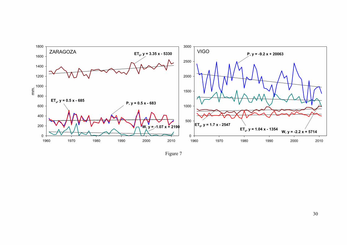
30

Figure 7

ZARAGOZA

1960 1970 1980 1990 2000 2010

mm.

0

200

400

600

800

1000

1200

1400

1600

1800

ET0, y = 3.35 x - 5330

ETa, y = 0.5 x - 685 P, y = 0.5 x - 683

W, y = -1.07 x + 2190

VIGO

1960 1970 1980 1990 2000 20100

500

1000

1500

2000

2500

3000

ET0, y = 1.7 x - 2547ETa, y = 1.04 x - 1354

P, y = -9.2 x + 20063

W, y = -2.2 x + 5714

31

Figure 8

SPEI

1960 1970 1980 1990 2000 2010-3

-2

-1

0

1

2

3

Standardized (P-ETa)

1960 1970 1980 1990 2000 2010-3

-2

-1

0

1

2

3

Standardized (ETa-PET)

1960 1970 1980 1990 2000 2010-3

-2

-1

0

1

2

3

SPEI

1960 1970 1980 1990 2000 2010-3

-2

-1

0

1

2

3

Standardized (P-ETa)

1960 1970 1980 1990 2000 2010-3

-2

-1

0

1

2

3

Standardized (ETa-PET)

1960 1970 1980 1990 2000 2010-3

-2

-1

0

1

2

3

ZARAGOZA VIGO

32

A)

B)

Figure 9

-1 -0

SP

EI

-3

-2

-1

0

1

2

3

-1 -0

SP

I

-3

-2

-1

0

1

2

3

-1 -0

st. (

P-E

T a)

-3

-2

-1

0

1

2

3

0 1 1 1 0

SP

EI

-2

-1

0

1

2

0 1 1 1 0

SP

I

-2

-1

0

1

2

0 1 1 1 0

st. (

P-E

T a)

-2

-1

0

1

2

33

A)

B)

Figure 10

1950 1955 1960 1965 1970 1975 1980 1985 1990 1995 2000 2005 2010

SP

EI

-3

-2

-1

0

1

2

3

1950 1955 1960 1965 1970 1975 1980 1985 1990 1995 2000 2005 2010

SP

I

-3

-2

-1

0

1

2

3

1950 1955 1960 1965 1970 1975 1980 1985 1990 1995 2000 2005 2010

st. (

P-E

T a)

-3

-2

-1

0

1

2

3

2007 2008 2009 2010 2011 2012

SP

EI

-2

-1

0

1

2

2007 2008 2009 2010 2011 2012

SP

I

-2

-1

0

1

2

2007 2008 2009 2010 2011 2012

st. (

P-E

T a)

-2

-1

0

1

2

34

Figure 11

1900 1910 1920 1930 1940 1950 1960 1970 1980 1990 2000 2010

SPEI

-3-2-10123

1900 1910 1920 1930 1940 1950 1960 1970 1980 1990 2000 2010

SPEI

-3-2-10123

1900 1910 1920 1930 1940 1950 1960 1970 1980 1990 2000 2010

SPEI

-3-2-10123

1900 1910 1920 1930 1940 1950 1960 1970 1980 1990 2000 2010

SPEI

-101

1900 1910 1920 1930 1940 1950 1960 1970 1980 1990 2000 2010

SPEI

-101

1900 1910 1920 1930 1940 1950 1960 1970 1980 1990 2000 2010

SPEI

-101

(Th)

(Hg)

(Pm)

(Hg-Th)

(Pm-Th)

(Pm-Hg)

35

Figure 12

(Th)

1960 1965 1970 1975 1980 1985 1990 1995 2000 2005 2010

SPEI

-3-2-10123

(Hg)

1960 1965 1970 1975 1980 1985 1990 1995 2000 2005 2010

SPEI

-3-2-10123

(Pm)

1960 1965 1970 1975 1980 1985 1990 1995 2000 2005 2010

SPEI

-3-2-10123

(Hg-Th)

1960 1965 1970 1975 1980 1985 1990 1995 2000 2005 2010

SPEI

-101

(Pm-Th)

1960 1965 1970 1975 1980 1985 1990 1995 2000 2005 2010

SPEI

-101

(Pm-Hg)

1960 1965 1970 1975 1980 1985 1990 1995 2000 2005 2010

SPEI

-101

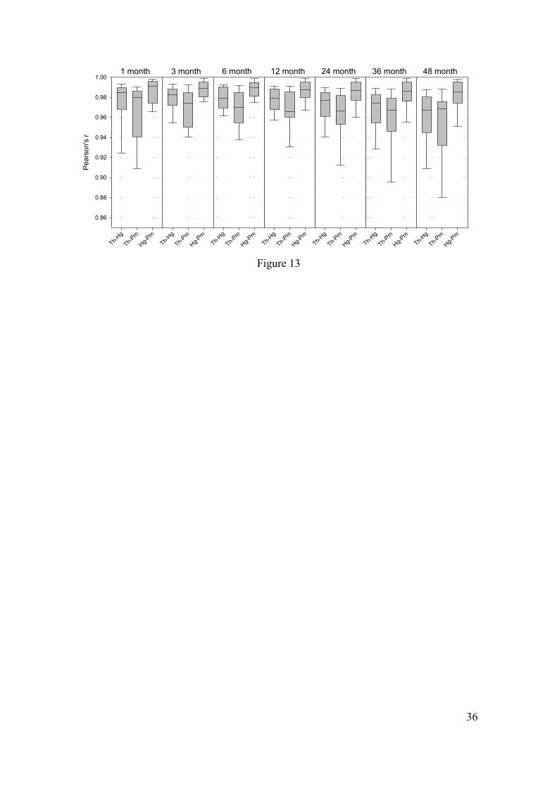
36

Figure 13

1 month

Th-Hg

Th-Pm

Hg-Pm

Pea

rson

's r

0.86

0.88

0.90

0.92

0.94

0.96

0.98

1.003 month

Th-Hg

Th-Pm

Hg-Pm

6 month

Th-Hg

Th-Pm

Hg-Pm

12 month

Th-Hg

Th-Pm

Hg-Pm

24 month

Th-Hg

Th-Pm

Hg-Pm

36 month

Th-Hg

Th-Pm

Hg-Pm

48 month

Th-Hg

Th-Pm

Hg-Pm

37

Figure 14

1 month

Th Hg

Mea

n A

bsol

ute

Diff

eren

ce

0.0

0.1

0.2

0.3

0.4

0.53 month

Th Hg

6 month

Th Hg

12 month

Th Hg

24 month

Th Hg

36 month

Th Hg

48 month

Th Hg

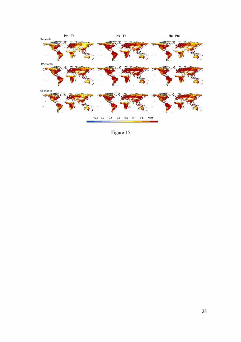
38

Figure 15

39

Figure 16

3 month

Th-Hg

Th-Pm

Hg-Pm

Pea

rson

's r

0.4

0.5

0.6

0.7

0.8

0.9

1.012 month

Th-Hg

Th-Pm

Hg-Pm

48 month

Th-Hg

Th-Pm

Hg-Pm

40

Figure 17

41

Figure 18

3 month

Th Hg

Mea

n A

bsol

ute

Diff

eren

ce

0.0

0.2

0.4

0.6

0.8

1.012 month

Th Hg

48 month

Th Hg

42

Figure 19

Annual precipitation (mm.)

200 400 600 800 1000 1200 1400 1600 1800

R-P

ears

on (T

h vs

. Pm

)

0.92

0.94

0.96

0.98

1.00

Annual precipitation (mm.)

200 400 600 800 1000 1200 1400 1600 1800

R-P

ears

on (T

h vs

. Hg)

0.92

0.94

0.96

0.98

1.00

Annual precipitation (mm.)

200 400 600 800 1000 1200 1400 1600 1800

R-P

ears

on (P

m v

s. H

g)

0.92

0.94

0.96

0.98

1.00

Annual temperature (ºC)

8 10 12 14 16 18 20

R-P

ears

on (T

h vs

. Pm

)

0.92

0.94

0.96

0.98

1.00

Annual temperature (ºC)

8 10 12 14 16 18 20

R-P

ears

on (T

h vs

. Hg)

0.92

0.94

0.96

0.98

1.00

Annual temperature (ºC)

8 10 12 14 16 18 20

R-P

ears

on (P

m v

s. H

g)

0.92

0.94

0.96

0.98

1.00

Rho = 0.74 Rho = 0.60 Rho = 0.64

Rho = -0.14 Rho = -0.07 Rho = -0.43

43

Figure 20

44

Figure 21

1 month

ThPm Hg

SP

EI c

hang

e de

cade

-1

-0.6

-0.4

-0.2

0.0

0.23 month

ThPm Hg

6 month

ThPm Hg

12 month

ThPm Hg

24 month

ThPm Hg

36 month

ThPm Hg

48 month

ThPm Hg

45

Figure 22

46

Figure 23

3 month

Th Pm Hg

SP

EI c

hang

e de

cade

-1

-0.3

-0.2

-0.1

0.0

0.1

0.212 month

Th Pm Hg

48 month

Th Pm Hg

3 month

Th Pm Hg

12 month

Th Pm Hg

48 month

Th Pm Hg

A) World B) Spain and the Netherlands

47

Figure 24

48

Figure 25

Rectangular

1960 1965 1970 1975 1980 1985 1990 1995 2000 2005 2010

SPEI

-3-2-10123

Triangular

1960 1965 1970 1975 1980 1985 1990 1995 2000 2005 2010

SPEI

-3-2-10123

Circular

1960 1965 1970 1975 1980 1985 1990 1995 2000 2005 2010

SPEI

-3-2-10123

Gaussian

1960 1965 1970 1975 1980 1985 1990 1995 2000 2005 2010

SPEI

-3-2-10123