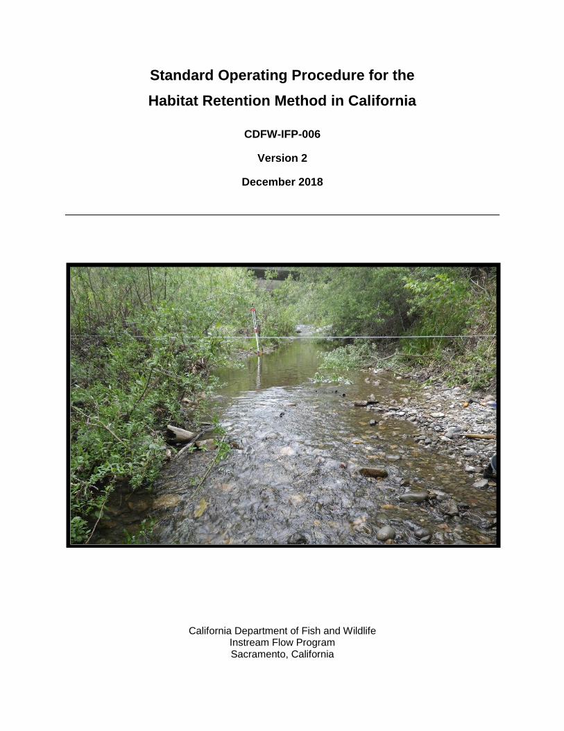
Standard Operating Procedure for the

Habitat Retention Method in California

CDFW-IFP-006

Version 2

December 2018

California Department of Fish and Wildlife Instream Flow Program Sacramento, California

2

Standard Operating Procedure for the

Habitat Retention Method in California

CDFW-IFP-006

Version 2

Approved by:

Robert Holmes, California Department of Fish and Wildlife, Statewide Water Planning Program

Manager, December 17, 2018

Beverly H. van Buuren, Quality Assurance Program Manager, December 17, 2018

Prepared by:

Originally prepared by Jason Hwan, California Department of Fish and Wildlife Instream Flow

Program, June 30, 2016; and revised by Danielle Ingrassia, California Department of Fish and

Wildlife Instream Flow Program, December 17, 2018

Suggested Citation:

CDFW. 2018. Standard Operating Procedure for the Habitat Retention Method in California.

California Department of Fish and Wildlife Instream Flow Program Standard Operating

Procedure CDFW-IFP-006, 33 p.

Available from: https://www.wildlife.ca.gov/Conservation/Watersheds/Instream-Flow/SOP

3

Table of Contents

Suggested Citation ..................................................................................................................... 2

List of Tables ............................................................................................................................. 4

List of Figures ............................................................................................................................ 4

Abbreviations and Acronyms ...................................................................................................... 5

Conversions ............................................................................................................................... 5

Acknowledgements .................................................................................................................... 6

Introduction ................................................................................................................................ 7

Scope of Application ............................................................................................................... 7

What is the Habitat Retention Method? .................................................................................. 8

Method Overview ..................................................................................................................12

Section 1: Field Work Preparation and Considerations .............................................................14

1.1 Method Limitations and Constraints .................................................................................14

1.2 Method Application ..........................................................................................................15

1.3 Site Selection ..................................................................................................................15

Section 2: Field Procedures ......................................................................................................16

2.1 Equipment List ................................................................................................................18

2.2 Data Collection ................................................................................................................18

Section 3: Data Analysis ...........................................................................................................21

3.1 Developing the Habitat Retention Rating Curve ...............................................................21

3.2 Interpreting the Results ....................................................................................................27

Glossary....................................................................................................................................30

References ...............................................................................................................................31

4

List of Tables

Table 1. Key flow parameters used to determine flow criteria using the habitat retention method

in riffle habitats ........................................................................................................................... 9

Table 2. Depth criteria for adult and juvenile salmonid passage to be used with the habitat

retention method. ......................................................................................................................11

Table 3. Example HRM transect habitat maintenance flows and hydraulic parameters for

scenarios 1-2 ............................................................................................................................28

Table 4. Example HRM transect habitat maintenance flows and hydraulic parameters for

scenario 3 .................................................................................................................................29

List of Figures

Figure 1. Conceptualized longitudinal profile of a pool-riffle sequence showing the location of the

hydraulic control. .......................................................................................................................10

Figure 2. Conceptualized cross-section of a stream channel highlighting the bankfull width for

use with the habitat retention method ........................................................................................12

Figure 3. Example of a transect across the hydraulic control at the top of a riffle ......................16

Figure 4. Example of staff gage used to assess changes in WSEL during surveys. ..................21

Figure 5. Example HRM transect data uploaded into HydroCalc (Molls 2010) for rating curve

generation. ................................................................................................................................23

Figure 6. Example HRM transect HydroCalc (Molls 2010) cross-section plot and bankfull wetted

edge location identification. .......................................................................................................24

Figure 7. Example rating curve computation using HydroCalc (Molls 2010). .............................26

5

Abbreviations and Acronyms

Term Definition

BMI Benthic macroinvertebrate

cfs Cubic feet per second

cm Centimeter

Department California Department of Fish and Wildlife

ft Feet/foot

ft/s Feet per second

GPS Global positioning system

HP Headpin

HRM Habitat retention method

IFP Instream Flow Program

in. Inch

LBWE Left bank wetted edge

m Meter

PHABSIM Physical habitat simulation

QA Quality assurance

QC Quality control

RBWE Right bank wetted edge

s Second

SOP Standard operating procedure

TP Tailpin

USGS U.S. Geological Survey

VBM Vertical benchmark

WSEL Water surface elevation

Conversions

1 cfs ≈ 2.83 × 10-2 m3/s 1 in. = 2.54 cm 1 ft = 0.3048 m

6

Acknowledgements

This document was completed with assistance from the California Department of Fish and

Wildlife (Department) Water Branch Instream Flow Program (IFP) staff, including William

Cowan, Diane Haas, Jason Hwan, Bronwen Stanford, Paige Uttley, and Amber Villalobos. The

authors are grateful for the external technical review provided by the Instream Flow Council and

the Quality Assurance Services Group in the Marine Pollution Studies Laboratory at Moss

Landing Marine Laboratories.

7

Introduction

This standard operating procedure (SOP) represents the protocol for habitat retention method

(HRM) studies conducted by the Department IFP. It is intended to replace the original 2016

SOP. It may be used in conjunction with other IFP SOPs. The overall concept of this SOP is

based on information found in Hydraulic Simulation in Instream Flow Studies: Theory and

Techniques (Bovee and Milhous 1978) and Evaluation of Instream Flow Methods and

Determination of Water Quantity Needs for Streams in the State of Colorado (Nehring 1979).

Instructions are provided for:

• Preparation and considerations for field work

o HRM limitations and constraints

o Method application

o Site selection

• Data collection

o Equipment list

o Field procedures

• Data Analysis

o Habitat retention rating curve development

o Rating curve results interpretation

Scope of Application

This SOP provides the procedural reference for Department staff conducting the HRM, when

site conditions and research objectives indicate that the HRM is an appropriate method. For

example, the HRM is used to evaluate habitat maintenance flows at riffle sites that contain

hydraulic bed controls. This SOP is intended as an informational resource for other state and

federal agencies, nongovernmental organizations, private contractors, and other organizations

throughout California.

The HRM method is used to identify habitat maintenance flows that maintain hydraulic criteria

for average depth, average velocity, and wetted perimeter, at the hydraulic control of a riffle.

These three parameters are good indicators of flow-related stream habitat quality. The HRM

quantifies the minimum flow sufficient to provide a basic survival level for fish during times of the

year when streamflow is at its lowest (Annear et al. 2004). Use of the HRM for fish and wildlife

includes the following considerations:

8

• Transect locations must be at hydraulic control points of riffles.

• The method is only useful for identifying threshold flows for hydraulic parameters (i.e.,

depth, velocity, and wetted perimeter).

• The method is limited to streams with a bankfull width of 100 ft or less.

• The method is not suitable for complex channels.

• There is a limited ability to identify trade-offs between different flow levels and habitat

suitability for various aquatic organisms.

• Other methods and/or models are needed to assess flow requirements for other riverine

elements such as channel geomorphology, riparian vegetation, or water quality.

There are two main approaches to conducting hydraulic control based habitat methods such as

the HRM. Both approaches require data to be collected along the hydraulic control of a

representative alluvial riffle. The field-based approach requires a minimum of 10 site visits at

prescribed flow events to generate hydraulic habitat relationships. The modelling approach uses

a surveyed bed profile, paired with a flow measurement, and a computer program based on

Manning’s equation to develop hydraulic habitat relationships.

This SOP focuses on describing HRM data collection and analysis using the modeling

approach. It provides an overview of rating curve development but does not describe hydraulic

modelling in depth to account for user discretion in selecting a computer program based on

Manning’s equation. The Department encourages SOP users to contact the IFP with any

questions or for assistance with project planning. The Department is not responsible for

inappropriate application or inaccurate interpretation of the HRM SOP. The Department highly

recommends that an experienced instream flow practitioner conduct all field work and data

analysis.

Note: Safety is a primary concern when conducting instream flow studies. Conduct sampling

only when field conditions are safe.

What is the Habitat Retention Method?

The HRM is a site-specific method used in riffle habitats to identify habitat maintenance flows

that allow for the movement and long-term persistence of aquatic biota. Riffles are characterized

by shallow habitats with relatively fast velocities compared to pools or glides. As such, riffles

tend to generate high concentrations of dissolved oxygen, and consist of substrates (i.e., gravel

9

and cobble) that are well-suited for the production of benthic macroinvertebrates (BMI) and

spawning of many species of salmonids. Additionally, smaller fish may seek refuge in riffles to

avoid larger predatory fish that inhabit deeper habitats (e.g., pools). As a result of their shallow

depths, riffles (and their hydraulic parameters) are more sensitive to changes in stream flow

than other habitat types (e.g., pools, runs, and glides). Diminishing flow at riffles can in turn limit

fish passage, including anadromous salmonid ocean outmigration or upstream spawning

migration. Dewatering of riffles decreases BMI productivity during the summer and may also

limit pool-to-pool movements of juvenile fishes.

For the purposes of this SOP, habitat maintenance flows are defined as the amount of

continuous flow in cubic feet per second (cfs) required to maintain hydraulic criteria for average

depth, average velocity, and percent wetted perimeter (described in Table 1) at the hydraulic

control of riffles (depicted in Figure 1). These hydraulic criteria vary depending on the species

and life stage of fish that frequent or reside in the stream, as well as the stream width. The

criteria for average depth increases proportionally to stream width, considered the bankfull

width, due to the assumption that larger streams support larger fish, which require greater

passage depths (R.B. Nehring, pers. comm., October 1, 2018).

Table 1. Key flow parameters used to determine flow criteria, using the habitat retention method in riffle habitats. Percent wetted perimeter is relative to bankfull conditions.1

Bankfull width (ft)

Average depth (ft)

Average velocity (ft/s)

Wetted perimeter (%)

1−20 0.2 1 50

21−40 0.2−0.4 1 50

41−60 0.4−0.6 1 50−60

61−100 0.6−1.0 1 70

1 Table and values are adopted from Nehring (1979).

10

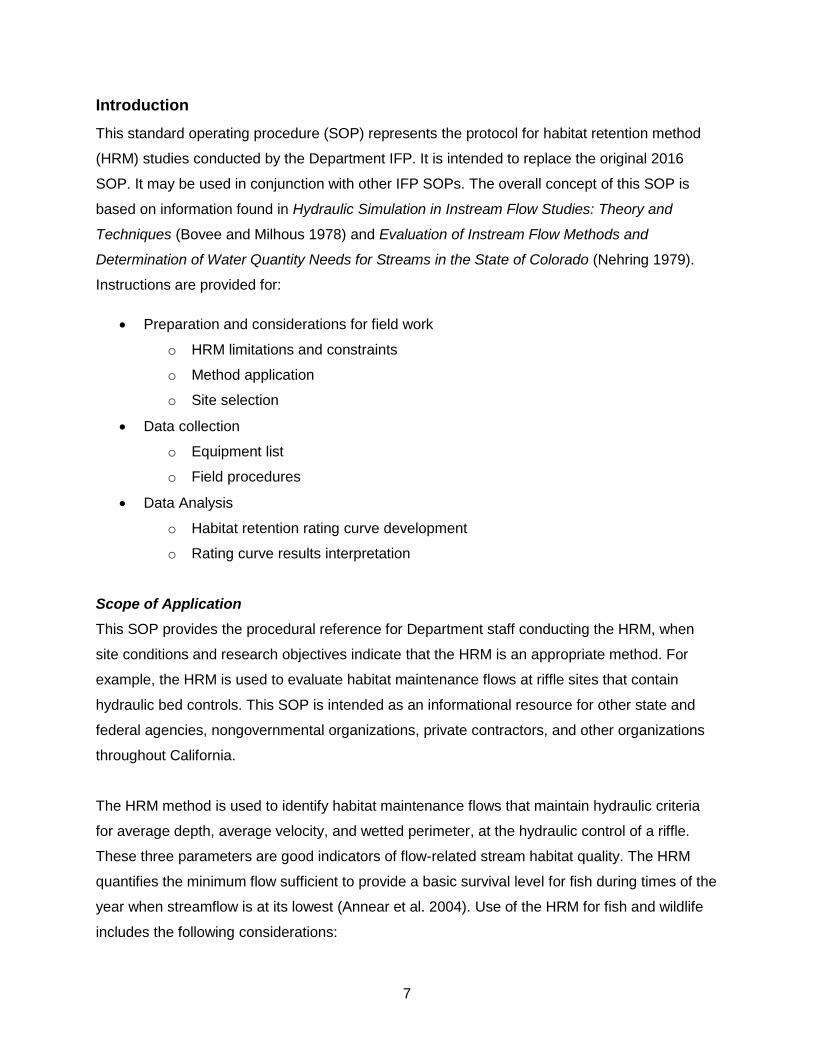
Figure 1. Conceptualized longitudinal profile of a pool-riffle sequence showing the location of the hydraulic control.

A key assumption of the HRM is that if hydraulic criteria are maintained in riffle habitats,

adequate flow conditions will also be maintained for other habitat types, such as pools and runs,

located in the same stream reach (Nehring 1979). Though each criterion is important, the depth

criterion must always be met in addition to at least one of the other criteria. The average depth

criterion for streams up to 20 ft in width is 0.2 ft (Table 1). For streams that are wider than 20 ft,

bankfull width is multiplied by 0.01 to determine the average depth criterion. For example, if a

stream is 28 ft wide, the average depth criterion is 0.28 ft.

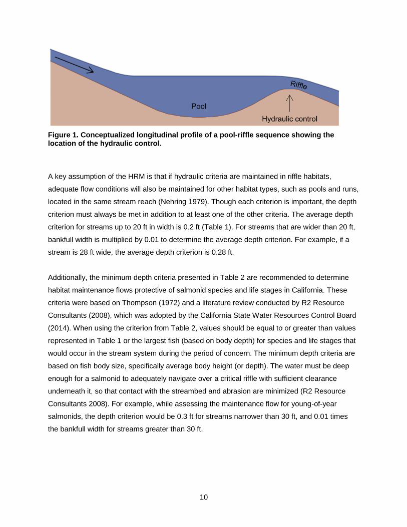
Additionally, the minimum depth criteria presented in Table 2 are recommended to determine

habitat maintenance flows protective of salmonid species and life stages in California. These

criteria were based on Thompson (1972) and a literature review conducted by R2 Resource

Consultants (2008), which was adopted by the California State Water Resources Control Board

(2014). When using the criterion from Table 2, values should be equal to or greater than values

represented in Table 1 or the largest fish (based on body depth) for species and life stages that

would occur in the stream system during the period of concern. The minimum depth criteria are

based on fish body size, specifically average body height (or depth). The water must be deep

enough for a salmonid to adequately navigate over a critical riffle with sufficient clearance

underneath it, so that contact with the streambed and abrasion are minimized (R2 Resource

Consultants 2008). For example, while assessing the maintenance flow for young-of-year

salmonids, the depth criterion would be 0.3 ft for streams narrower than 30 ft, and 0.01 times

the bankfull width for streams greater than 30 ft.

11

Table 2. Depth criteria for adult and juvenile salmonid passage to be used with the habitat retention method.

Species Minimum depth (ft)

Steelhead (adult) 0.7

Coho salmon (adult) 0.7

Chinook salmon (adult) 0.9

Trout (adult, including age 1-2+ juvenile steelhead) 0.4

All salmonids (young-of-year juvenile) 0.3

The bankfull elevation is used to identify bankfull width, and bankfull discharge. It is also used to

calculate percent wetted perimeter. The bankfull elevation determination is an integral

component in the development of habitat maintenance flows. IFP follows bankfull identification

processes outlined by Leopold et al. (1964), Rosgen (1994), and the Colorado Water

Conservation Board (CWCB; 2006). For the purposes of this SOP, bankfull elevation is

determined using the following indicators:

1. Top of point bars

2. Change in the lower limit of perennial vegetation

3. Change in slope from slope to vertical or vice versa

4. Change in substrate particle size

5. Bank undercuts; and/or

6. Stain lines (Harrelson et al. 1994)

All indicators need not be present and not necessarily identified in this order. The bankfull

elevation, as depicted in Figure 2, can be recognized by physical indicators along the stream

bank. Elevation is generally located below sedges and other plants that may survive submerged

under high flows (CWCB 2006). Special considerations may be necessary when working in

intermittent and ephemeral streams where bankfull stage indicators may be less defined

(USACE 2012).

12

Figure 2. Conceptualized cross-section of a stream channel highlighting the bankfull width for use with the habitat retention method. Note: Bankfull conditions commonly occur at elevations where there are visible changes in channel slope, vegetation, and/or substrate.

Method Overview

Cross-sectional transects are established at the hydraulic control point of riffles. It is essential

that the transect be placed on the apex of the controlling bed element. It is not appropriate to

simply place the transect anywhere in a shallow riffle as the hydraulic criteria generated at those

points will differ from the precise control feature. The bankfull width of the stream (which is

necessary for determining the percent of wetted perimeter) is measured along the transect at

the bankfull elevation using a fiberglass measuring tape.

Bed elevation readings are obtained along the stream channel cross-section using an

engineering level, such as an auto level (see the Standard Operating Procedure for Streambed

and Water Surface Elevation Data Collection in California (CDFW 2013c)). Hydraulic slope is

also estimated by measuring the riffle length and taking water surface elevations (WSELs) at

the upstream and downstream extent of each riffle mesohabitat unit. A discharge measurement

must be recorded for each HRM transect. A single discharge may be used for all transects that

are located in the same reach if it is free of physical obstructions, tributaries, or diversions

between each HRM transect, and discharge remains consistent across sites. Discharge is

measured in the reach and near the site using a flow meter and top-setting wading rod (see the

Standard Operating Procedure for Discharge Measurements in Wadeable Streams in California

13

(CDFW 2013a)). Discharge may also be obtained from a nearby representative stream gage.

An applicable stream gage must have no physical obstructions, tributaries, or diversions

between the gage location and the HRM transect(s) in the reach.

Bed elevation and WSEL data are used to calculate the flow area (A), wetted perimeter, and

hydraulic radius (R) each transect. Based on the 'constant shear stress at the boundary'

assumption (Khiadani et al. 2005), hydraulic radius is defined as the ratio of the channel's cross-

sectional area of the flow to its wetted perimeter (i.e. the portion of the cross-section's perimeter

that is "wet"). WSEL and riffle length are used to estimate hydraulic slope (S); and velocity and

cross-sectional area data are used to estimate discharge (Q). These values are then used to

calculate Manning’s roughness coefficient (n) using the Manning’s equation for open channel

flow (Gupta 2008):

𝐸𝑞𝑢𝑎𝑡𝑖𝑜𝑛 1: 𝑛 = (1.486

𝑄) 𝐴𝑅

2

3𝑆1

2 (English units)

The calculated values for discharge, hydraulic slope, and Manning’s roughness coefficient,

along with the bed elevation data collected in the field, are used as inputs to create rating

curves between discharge and average hydraulic depth, average flow velocity, and wetted

perimeter. When HRM criteria (Table 1) for depth and at least one other parameter are met,

flows are deemed to be suitable for aquatic macroinvertebrate survival and the long-term

persistence of aquatic biota. Furthermore, when species and life stage-specific HRM criteria

(Table 2) for depth and at least one other parameter are met, flows are deemed to be suitable

for movement of the selected salmonid species and life stage.

Hydraulic parameters are modeled over a range of flows based on a single field flow

measurement and the estimated Manning’s roughness coefficient. It is recommended that when

using hydraulic models, two or more additional site visits at different discharges are taken to

compare field observations with model outputs (Annear et el. 2004). The Department IFP

employs a computer program based on Manning’s equation to model hydraulic parameters,

though other programs are available. Depending on the computer program selected for

analysis, data collection requirements may differ. Review the data input requirements of the

selected model before beginning field data collection.

14

Section 1: Field Work Preparation and Considerations

HRM surveys should be conducted by at least two practitioners who have experience with

standard surveying equipment for collecting streambed and WSEL data as well as discharge

measurements. The Department SOPs on streambed and WSEL data collection (CDFW 2013c)

and discharge measurements (CDFW 2013a) are available on the Department’s IFP website.

Contact Department IFP staff for project planning and method assistance.

For calculating habitat maintenance flows using Manning’s equation, it is important for an

experienced practitioner to survey sites when flow is near the anticipated maintenance flow (see

Section 1.2: Method Application). The Manning’s equation best predicts the target hydraulic

parameters when the channel section is surveyed close to the target flow stage (i.e., near the

anticipated maintenance flow). Determining the approximate maintenance flow at the time of

survey may be difficult. Flow duration analysis may be used to help guide the timing of field

surveys (see the Standard Operating Procedure for Flow Duration Analysis in California (CDFW

2013b)). In some cases, it may take multiple surveys to capture field data at the approximate

maintenance flow. If field surveys are taken at the same HRM transect at multiple flows, each

survey event will require collection of corresponding slope measurements.

Crew safety is of paramount importance; only perform fieldwork when crews can safely survey.

1.1 Method Limitations and Constraints

The HRM is used to identify flows required to maintain hydraulic habitat conditions suitable for

maintenance of aquatic biota at different life stages. According to Annear et al. (2004), the

method’s main limitations are: by assuming hydraulic habitat as a surrogate for addressing the

biology of a stream, other ecological components are not considered; site selection and transect

placement must be performed by an experienced practitioner in order to yield appropriate flow

prescriptions; and analysis results in a single flow prescription per site thereby omitting flow

needs for intra- and inter-annual variability.

15

1.2 Method Application

For maximum viability of the results, collect HRM data when instream flow is near the

anticipated maintenance flow. In alluvial channels, the Manning’s roughness coefficient is

particularly sensitive to changes in WSEL and is generally much higher during low-flow

conditions when compared to high flow conditions (Limerinos 1970; George and Schneider

1989). As such, the streambed should be watered at the toe of each bank to avoid transects

containing dry portions of streambed. Additionally, flows close to the maintenance flow will limit

the likelihood of obtaining erroneous estimates of hydraulic parameters for model simulations

using the Manning’s equation. The IFP recommends that the simulated flow range is between

0.4 and 2.5 times the survey flow, which is generally consistent with the recommended flow

range for physical habitat simulation (PHABSIM) models (Milhous et al. 1984).

1.3 Site Selection

Within a river reach, target a minimum of three representative riffles with roughly rectangular

beds (as opposed to V-shaped channels) for the HRM. A sample size of at least three is

required to calculate a statistically significant variance and allows for channel morphology

comparability. Select riffle sites that are representative of the overall geomorphic structure and

shape of the river reach. For each riffle surveyed, the transect must be located at the hydraulic

control, which is typically located at the riffle crest (see Figures 1 and 3). Streamflow should be

uniform across the transect to maximize the reliability of Manning’s equation (Grant et el. 1992).

The transect location should have natural banks or grasslines, not eroding or undercut banks,

and be free from braiding (CWCB 2006).

Note: While selecting riffles, beware of redds (e.g., salmonid, lamprey) that may be present.

Avoid and place transects away from redds.

16

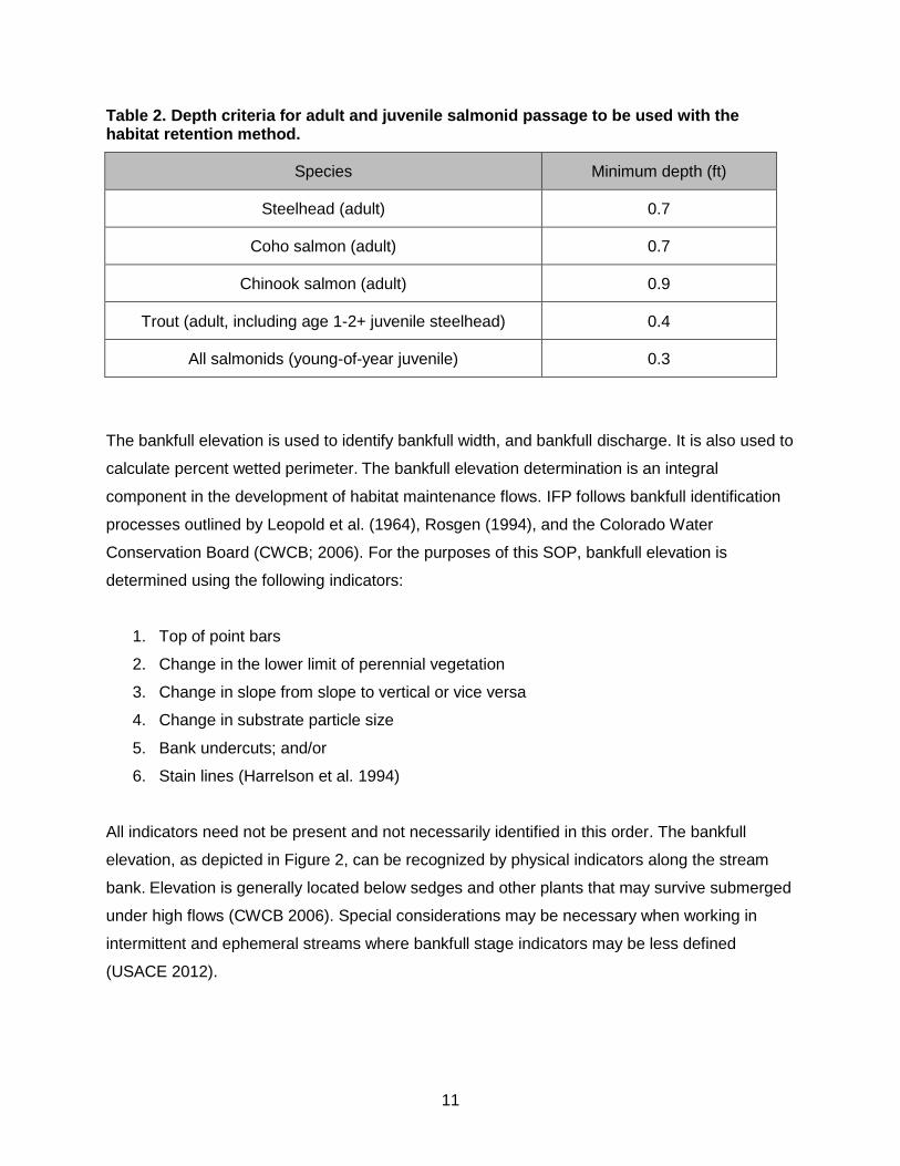
Figure 3. Example of a transect across the hydraulic control at the top of a riffle. Photo

taken facing upstream.

Section 2: Field Procedures

Establish transect locations as specified by this SOP. At each transect, install a headpin (HP)

and tailpin (TP) on the left bank and right bank, respectively. Install the HP and TP as high up

on the bank as possible. The left and right banks are designated while facing upstream.

Measure the bankfull width (see Method Overview) and wetted width (distance between left

bank and right bank wetted edges). Install a vertical benchmark (VBM). Bed and WSEL data are

surveyed using a stadia rod at multiple stations located along the measuring tape that is

stretched from HP to TP. Stations are selected to include representation of streambed features,

including the deepest point and each location with a distinct change in channel topography.

HRM transects within the river reach must be accompanied by a representative discharge

measurement to develop discharge rating curves. If an operational stream gage is located near

enough to the transect to negate stream gains and losses, discharge may be obtained from the

stream gage as opposed to measuring discharge directly. Practitioners must understand and

identify the limitations and accuracy of the stream gage selected for use with the HRM. For

17

example, U.S. Geological Survey (USGS) operates stream gages that are accurate to the

nearest 0.01 ft or 0.2 percent of stage, whichever is greater (Olson and Norris 2007).

If measuring discharge in the field, collect the discharge data from a nearby site suitable for

measuring discharge (see the Standard Operating Procedure for Discharge Measurements in

Wadeable Streams in California (CDFW 2013a). Depths are measured to the nearest 0.05 ft.

Distances between measurements should be set so that less than 5% of the entire flow

measured, and no more than 10% (Turnipseed and Sauer 2010), passes between any two

adjoining measurement locations along the transect. Generally, at least 20 velocity and depth

measurements are needed along each transect. A single good quality discharge site can be

used for multiple HRM transects if there are no inputs or diversions between transect locations

and the flow measurement is representative of each HRM transect flow.

18

2.1 Equipment List 2

Auto level

Bucket for flow meter calibration

Camera

Clipboard

Flagging tape

Flow meter

Gloves

GPS unit

Hammer

Hearing protection

Lag bolt (for VBM)

Loppers (if needed to remove vegetation)

Pencils

Permanent marker

Rebar (two per transect) and safety caps

Rite-in-the Rain field data sheets or notebook

Stadia rod (engineering grade rod capable of measuring 1/10 ft and 1/100 ft)

Staff gage

Two fiberglass measuring tapes

Tripod

USGS top-setting wading rod

2.2 Data Collection

Step 1: Insert the staff gage into the substrate near the stream’s edge, near the transect, and

out of the foot traffic path (see Figure 4). Record gage height to the nearest 0.01 in. immediately

before and after data collection to account for any fluctuations in water surface height that may

occur during data collection. If the gage height changes more than 0.02 in. during data

collection, the measurements need to be retaken when water levels stabilize (see the Standard

Operating Procedure for Streambed and Water Surface Elevation Data Collection in California

(CDFW 2013c)).

2 Calibrate the flow meter and auto level according to manufacturer’s instructions prior to use.

19

Step 2: During the field survey, establish each transect identified during the site selection

process (outlined in Section 1.3: Site Selection):

• Establish the transect HP and TP on the stream banks so that the measuring tape is

level and is located across the apex of the riffle’s hydraulic control. Install the HP and TP

by hammering in rebar on the left and the right banks, respectively. The HP and TP must

be installed above bankfull to ensure that the left and right bankfull locations can be

identified and recorded along the transect tape.

• Install the VBM, in this case a lag bolt, on a permanent, unmovable point (see the

Standard Operating Procedure for Streambed and Water Surface Elevation Data

Collection in California (CDFW 2013c)).

• Mark GPS waypoints at the HP, TP, and VBM, and record the corresponding waypoints.

Step 3: String the fiberglass measuring tape across the transect from HP to TP creating a taut,

level, and straight line with the measuring tape. Starting at 0 ft, record the total distance from HP

to TP. Record the distances on the measuring tape to the nearest 0.1 ft where the left bank

wetted edge (LBWE) and right bank wetted edge (RBWE) occur. Additionally, record the

distances on the measuring tape where bankfull conditions occur on the left bank and right bank

to the nearest 0.1 ft. Take photos, notes, and sketches to identify changes in slope, substrate,

and vegetation to support the identification of the bankfull elevation in the field.

Step 4: Photograph the transect facing upstream and downstream and ensure that the left bank

and right bank are visible in each photo. Take additional photos of the left and right bank

capturing the indicators (see What is the Habitat Retention Method?). Photos taken in the field

can be used to help determine bankfull locations prior to data analysis. Ensure that the photos

are clear and record photo identification numbers.

Step 5: Set up the auto level in a location where the entire transect is within the line of sight of

the instrument, if possible. Otherwise, a turning point must be established to collect streambed

elevation data for the entire transect. Ensure that there is a clear line of sight between the auto

level and the VBM and HP locations. After recording the VBM elevation, collect and record

streambed elevation data at 1-ft increments from HP to TP, with additional measurements taken

at the lowest point at the thalweg and at any changes in slope, as needed. Take additional

20

elevation points along the transect to identify marked changes in slope, substrate, and

vegetation to support the identification of the bankfull elevation. Smaller or larger increments

may be allowed to accurately capture higher levels of bed complexity and to adhere to the goal

of representing all topographical change3. For detailed guidance on collecting streambed

elevation data, see the Standard Operating Procedure for Streambed and Water Surface

Elevation Data Collection in California (CDFW 2013c).

Step 6: At the transect, measure and record representative WSELs near the LBWE, RBWE, and

at the midchannel. At the downstream extent of the riffle, preceding changes in hydraulic slope,

measure and record representative WSELs at the midchannel and near the LBWE, RBWE as

needed. Measure and record the riffle length from the transect (i.e., upstream extent) to the

downstream extent where the WSELs were measured. These measurements will be used to

calculate hydraulic slope.4 Once all bed and WSEL data are collected, resurvey the VBM using

the auto level and stadia rod. Resurveying the VBM is a necessary check to ensure that the

auto level was stationary for the survey duration. For detailed guidance on collecting WSEL

data, see the Standard Operating Procedure for Streambed and Water Surface Elevation Data

Collection in California (CDFW 2013c).

Note: The upstream extent is located at the hydraulic control (i.e., on the transect) and the

downstream extent occurs at the bottom of the riffle mesohabitat unit, just upstream of the next

habitat unit and preceding changes in hydraulic slope.

Step 7: If measuring discharge in the field, find a suitable location to measure discharge in the

reach and near the HRM transect and establish a discharge transect. For detailed guidance on

measuring discharge, see the Standard Operating Procedure for Discharge Measurements in

Wadeable Streams in California (CDFW 2013a).

Step 8: After data collection is complete and data sheets are checked for completeness, remove

all survey equipment.

3 Increments greater than 1 ft may be appropriate in engineered channels, such as concrete-lined channels, with a relatively uniform cross-section. 4 An experienced practitioner may use professional judgment to determine the level of detail needed to accurately measure the change in hydraulic slope. For example, if the transect is located on a river bend and it is determined that WSELs on the left bank are more representative than measurements on the right bank, it may be acceptable to only take measurements in the representative areas.

21

Figure 4. Example of staff gage used to assess changes in WSEL during surveys.

Section 3: Data Analysis

3.1 Developing the Habitat Retention Rating Curve

Data may be entered and stored in a spreadsheet program such as Microsoft Excel in

preparation for analysis. Once all field data are entered and checked according to procedures

identified in the project study plan, development of rating curves and data analysis can

commence. Department IFP QA documents, including a study plan template, are available at

https://www.wildlife.ca.gov/Conservation/Watersheds/Instream-Flow/SOP. Please contact the

Department IFP for assistance.

The Department IFP uses the commercially available software NHC Hydraulic Calculator

(HydroCalc; Molls 2010), a computer program based on Manning’s equation, to model hydraulic

parameters and the stage-discharge relationship for cross-sectional transects. However, several

programs based on Manning’s equation are available and any can be used. For more guidance

on hydraulic modelling, please contact the Department IFP.

HydroCalc requires the survey discharge, hydraulic slope, and Manning’s n roughness

coefficient to develop the rating curve for each HRM transect site. Next, compare the hydraulic

22

parameters calculated from survey field data to the model output for validation. The following

steps can be used as general guidance for generating a rating curve using HRM survey data.

These steps are associated with HydoCalc. Steps may need to be altered if using a different

software program.

Step 1: Calculate the discharge measurement associated with the HRM transect following the

Standard Operating Procedure for Discharge Measurements in Wadeable Streams in California

(CDFW 2013a). A practitioner may choose to use discharge data from an operational stream

gage in place of a field discharge measurement (see Section 2: Field Procedures). The gage

data must be representative of conditions during the time of the HRM survey. The downloaded

gage data would be paired with the bed profile and WSEL survey data and used in place of a

field discharge measurement in HydroCalc for the transect HRM analysis. Gage data that would

be selected for pairing based off time and date of survey data of interest. Although it is

acceptable to use a gage discharge HRM analysis, the IFP recommends that a field discharge

measurement be taken, if feasible, to increase confidence in the modeled relationship between

the surveyed WSELs and flow.

Step 2: Surveyed streambed and WSEL data, collected in accordance with the Standard

Operating Procedure for Streambed and Water Surface Elevation Data Collection in California

(CDFW 2013c), convert from foresight measurements to elevations. This is done by subtracting

the foresight height from the height of the instrument. For purposes of HRM data collection, the

height of the instrument or instrument height is the VBM elevation, assumed to be 100 ft, plus

the VBM foresight height measured in the field.

Step 3: The hydraulic slope of the HRM riffle mesohabitat unit is calculated as the average

WSEL elevation measured at the hydraulic control minus the average WSEL elevation

measured at the downstream extent of the mesohabitat unit, divided by the average length of

the mesohabitat unit. Measure WSELs and unit lengths at representative points.

Step 4: Manning’s n is calculated using Equation 1 (see Method Overview). Area is calculated

as the wetted area of the HRM transect, using the bed elevation data. Hydraulic radius is

calculated as the area divided by wetted perimeter.

23

Step 5: Discharge, Manning’s n, slope, and the associated bed elevations for the HRM transect

are uploaded into HydroCalc (Figure 5). HydroCalc is then used to compute the HRM transect

parameters. To validate the rating curve, we recommend comparing the HydroCalc parameters

of area, wetted perimeter, hydraulic radius, and average WSEL to those calculated from the

transect survey data and used in the Manning’s n computation. The closer the predicted

transect parameters are to the field surveyed data, the stronger the relationship is between the

HydroCalc rating curve and the surveyed data. If the HydroCalc-predicted parameters differ

greatly from the values calculated with the surveyed data, the practitioner may want to use

transect data at a different flow or may need to omit a site from further analysis.

Figure 5. Example HRM transect data uploaded into HydroCalc (Molls 2010) for rating curve generation.

Step 6: Plot the validated HydroCalc cross-section parameters (Figure 6). The plot can be used

to determine the bankfull LBWE and RBWE identified in the field. Manually adjust the flow value

in HydroCalc until the water surface (blue line) is positioned where bankfull conditions are met.

24

The HydroCalc bankfull LBWE and RBWE locations (ft) along the transect should be recorded

and used to determine the bankfull width in ft. The bankfull width and associated flow are used

later in the HRM analysis.

Figure 6. Example HRM transect HydroCalc (Molls 2010) cross-section plot and bankfull wetted edge location identification.

Bankfull

LBWE

Bankfull

RBWE

25

Step 7: The rating curve is generated in HydroCalc by changing the flow back to the measured

discharge associated with the HRM transect, and by selecting Rating Curve. The flow range is

entered and must include the previously identified bankfull flow. The practitioner should take into

consideration that flow range entered doesn’t exceed the 0.4 and 2.5 thresholds for PHABSIM

models (Milhous et al. 1984). The number of data points selected by the practitioner will

determine the interval at which HydroCalc will model the transect’s stage-discharge relationship

(Figure 7). In the example, the transect’s rating curve will be generated at 1-cfs intervals from 1

to 50 cfs. When the practitioner saves the results of the rating curve, hydraulic parameters will

be predicted at each cfs interval.

26

Figure 7. Example rating curve computation using HydroCalc (Molls 2010).

27

3.2 Interpreting the Results

Record the HydroCalc rating curve hydraulic parameters in a spreadsheet program or notebook.

List average depth, average velocity, and percent wetted perimeter at each flow increment.

Percent wetted perimeter is calculated for each flow increment by dividing the predicted

incremental wetted perimeter by the wetted perimeter determined at bankfull flow.

The following three scenarios provide guidance on how to apply the HRM criteria. In each

scenario, the maintenance flow occurs when depth and at least one other hydraulic parameter

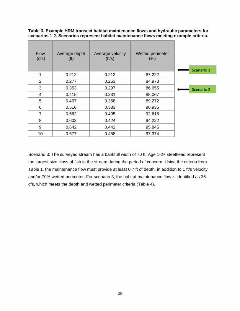
are met (Table 1). Table 3 represents rating curve hydraulic parameters for a hypothetical

stream with a 20-ft bankfull width. Table 4 represents rating curve hydraulic parameters for a

hypothetical stream with a 70-ft bankfull width.

Scenario 1: The surveyed stream has a bankfull width of 20 ft, and no salmonids are present.

When determining the habitat maintenance flow, reference the key flow parameters in Table 1.

The maintenance flow must provide at least 0.2 ft of depth, in addition to 1 ft/s velocity and/or

50% wetted perimeter. For scenario 1, the habitat maintenance flow is identified as 1 cfs, which

meets the depth and wetted perimeter criteria (Table 3).

Scenario 2: The surveyed stream has a bankfull width of 20 ft. Age 1-2+ steelhead represent

the largest size class of fish in the stream during the period of concern. For this scenario, the

maintenance flow is identified by using the depth criterion for a specific species and life stage of

interest, found in Table 2. The depth criterion for age 1-2+ steelhead is 0.4 ft. Therefore, the

maintenance flow must provide at least 0.4 ft of depth, in addition to 1 ft/s velocity and/or 50%

wetted perimeter. For scenario 2, the habitat maintenance flow is identified as 4 cfs, which

meets the depth and wetted perimeter criteria (Table 3).

28

Table 3. Example HRM transect habitat maintenance flows and hydraulic parameters for scenarios 1-2. Scenarios represent habitat maintenance flows meeting example criteria.

Flow (cfs)

Average depth (ft)

Average velocity (ft/s)

Wetted perimeter (%)

1 0.212 0.212 67.222

2 0.277 0.253 84.973

3 0.353 0.297 86.655

4 0.415 0.331 88.067

5 0.467 0.358 89.272

6 0.516 0.383 90.936

7 0.562 0.405 92.618

8 0.603 0.424 94.222

9 0.642 0.442 95.845

10 0.677 0.458 97.374

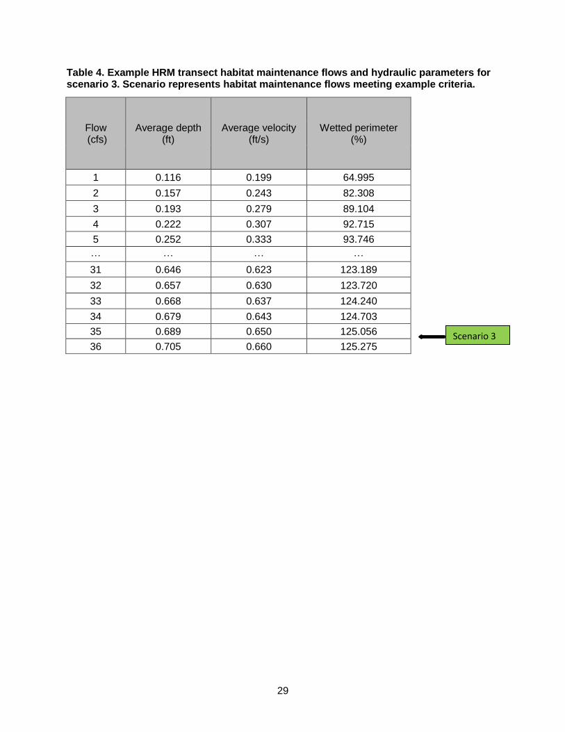
Scenario 3: The surveyed stream has a bankfull width of 70 ft. Age 1-2+ steelhead represent

the largest size class of fish in the stream during the period of concern. Using the criteria from

Table 1, the maintenance flow must provide at least 0.7 ft of depth, in addition to 1 ft/s velocity

and/or 70% wetted perimeter. For scenario 3, the habitat maintenance flow is identified as 36

cfs, which meets the depth and wetted perimeter criteria (Table 4).

Scenario 1

Scenario 2

29

Table 4. Example HRM transect habitat maintenance flows and hydraulic parameters for scenario 3. Scenario represents habitat maintenance flows meeting example criteria.

Flow (cfs)

Average depth (ft)

Average velocity (ft/s)

Wetted perimeter (%)

1 0.116 0.199 64.995

2 0.157 0.243 82.308

3 0.193 0.279 89.104

4 0.222 0.307 92.715

5 0.252 0.333 93.746

… … … …

31 0.646 0.623 123.189

32 0.657 0.630 123.720

33 0.668 0.637 124.240

34 0.679 0.643 124.703

35 0.689 0.650 125.056

36 0.705 0.660 125.275

Scenario 3

30

Glossary

Term Definition

Bankfull

The observed and identifiable location on each bank where change in slope, change in substrate, and/or lower limit of perennial vegetation occurs. Additional indicators include the top of point bars, bank undercuts, and stain lines. Elevation is generally located below sedges and other plants that may survive submerged under high flows.

Discharge The volume of water passing through a given cross-sectional area per unit time, typically expressed in cfs.

Habitat maintenance flows

The amount of continuous flow required to maintain hydraulic criteria for average depth, average velocity, and percent wetted perimeter at the hydraulic control of riffles.

Habitat retention method

Method for evaluating and identifying habitat maintenance flows that allow for the movement and long-term persistence of aquatic biota. Criteria for hydraulic parameters are based on Nehring (1979). Species- and life-stage-specific depth criteria are based on body depth requirements from Thompson (1972) and R2 Resource Consultants (2008), which were adopted by the California State Water Resources Control Board (2014).

Hydraulic control

A horizontal or vertical constriction in the channel, such as the crest of a riffle (Annear et al. 2004).

Toe of bank The break in slope at the foot of a streambank where the bank meets the streambed.

31

References

Annear, T., I. Chisholm, H. Beecher, A. Locke, P. Aarestad, C. Coomer, C. Estes, J. Hunt, R.

Jacobson, R. Jöbsis, J. Kauffman, J. Marshall, K. Mayes, G. Smith, R. Wentworth, and C.

Stalnaker. 2004. Instream flows for riverine resource stewardship. Revised Ed. Instream Flow

Council, Cheyenne, WY.

Bovee, K., and R. Milhous. 1978. Hydraulic simulation in instream flow studies: theory and

techniques. U.S. Fish and Wildlife Service, Instream Flow Information Paper 5.

CDFW. 2013a. Standard Operating Procedure for Discharge Measurements in Wadeable

Streams in California. California Department of Fish and Wildlife Instream Flow Program

Standard Operating Procedure CDFW-IFP-002, 24 p. Available from:

https://www.wildlife.ca.gov/Conservation/Watersheds/Instream-Flow/SOP

CDFW. 2013b. Standard Operating Procedure for Flow Duration Analysis in California.

Department of Fish and Wildlife Instream Flow Program Standard Operating Procedure

CDFWIFP-005, 17 p. Available from:

https://www.wildlife.ca.gov/Conservation/Watersheds/Instream-Flow/SOP

CDFW. 2013c. Standard Operating Procedure for Streambed and Water Surface Elevation Data

Collection in California. California Department of Fish and Wildlife Instream Flow Program

Standard Operating Procedure CDFW-IFP-003, 24 p. Available from:

https://www.wildlife.ca.gov/Conservation/Watersheds/Instream-Flow/SOP

CWCB. 2006. Development of Instream Flow Recommendations in Colorado Using R2CROSS

for Microsoft Excel. Colorado Water Conservation Board.

George, A.J.J., and V.R. Schneider. 1989. Guide for selecting Manning’s roughness coefficients

for natural channels and flood plains. U.S. Geological Survey Water-Supply Paper 2339.

Gupta, R. 2008. Hydrology and Hydraulic Systems. 3rd edition. Waveland Press, Long Grove,

IL.

Harrelson, C.C., C.L. Rawlins, and J.P. Potyondy. 1994. Stream channel reference sites: an

illustrated guide to field technique. General Technical Report RM-245. Department of

32

Agriculture, Forest Service, Rocky Mountain Forest and Range Experiment Station. Fort Collins,

CO: U.S. 61 p.

Khiadani, M.H., S. Beecham, J. Kandasamy, and M. Sivakumar. 2005. Boundary Shear Stress

in Spatially Varied Flow. Journal of Hydraulic Engineering 131:705–714.

Leopold, L., M. Wolman, and J. Miller. 1964. Fluvial processes in geomorphology. Dover

Publications, San Francisco, CA.

Limerinos, J.T. 1970. Determination of the Manning Coefficient From Measured Bed Roughness

in Natural Channels. U.S. Geological Survey Water-Supply Paper 1898-B.

Milhous, R., D. Wegner, and T. Waddle. 1984. User’s guide to the Physical Habitat Simulation

System (PHABSIM). Instream Flow Information Paper No. 11. U.S. Fish and Wildlife Service

FWS/ OBS-81/43.

Molls, T. 2010. HydroCalc. Version 3.0c (build 105). Available for download at

http://hydrocalc2000.com/download.php

Nehring, B.R. 1979. Evaluation of instream flow methods and determination of water quantity

needs for streams in the state of Colorado. Colorado Division of Wildlife.

Olson, S.A., and J.M. Norris. 2007. U.S. Geological Survey Streamgaging from the National

Stream Flow Information Program. U.S. Geological Survey. Pembroke, NH. Available from:

https://pubs.usgs.gov/fs/2005/3131/FS2005-3131.pdf

Rosgen, L.D. 1994. A classification of natural rivers. CATENA 22:169–199.

R2 Resource Consultants. 2008. Appendix G: Approach for Assessing Effects of Policy Element

Alternatives on Upstream Passage and Spawning Habitat Availability. Administrative Draft

prepared for the California State Water Resources Control Board, Division of Water Rights as

part of the North Coast Instream Flow Policy: Scientific Basis and Development of Alternatives

Protecting Anadromous Salmonids. March 14, 2008.

SWRCB. 2014. Policy for Maintaining Instream Flows in Northern California Coastal Streams.

Division of Water Rights, State Water Resources Control Board, California Environmental

Protection Agency. Sacramento, California. Available from:

http://www.waterboards.ca.gov/waterrights/water_issues/programs/instream_flows/

33

Thompson, K.E. 1972. Determining Streamflows for Fish Life. pp. 31-50 in Proceedings of the

Instream Flow Requirement Workshop. Pacific N.W. River Basins Commission. Portland, OR.

Turnipseed, D.P., and V.B. Sauer. 2010. Discharge measurements at gaging stations: U.S.

Geological Survey Techniques and Methods book 3, chap. A8, 87 p. Available from:

https://pubs.usgs.gov/tm/tm3-a8/pdf/tm3-a8.pdf

USACE. 2012. Field Identification of Ordinary High Water Mark in Relationship to the Field

Identification of Bankfull Stage for the Galveston District’s Tiered Stream Condition Assessment

Standard Operating Procedure. U.S. Army Corps of Engineers. Galveston, TX. Available from:

https://www.swg.usace.army.mil/