Embed Size (px)
Citation preview

ANSI/ASHRAE Addendum a toANSI/ASHRAE Standard 140-2001
Standard Method of Testfor the Evaluation ofBuilding Energy AnalysisComputer Programs
Approved by the ASHRAE Standards Committee on June26, 2004; by the ASHRAE Board of Directors on July 1,2004; and by the American National Standards Instituteon July 1, 2004.
This standard is under continuous maintenance by aStanding Standard Project Committee (SSPC) for whichthe Standards Committee has established a documentedprogram for regular publication of addenda or revisions,including procedures for timely, documented, consensusaction on requests for change to any part of the standard.The change submittal form, instructions, and deadlinesare given at the back of this document and may be ob-tained in electronic form from ASHRAE’s Internet HomePage, http://www.ashrae.org, or in paper form from theManager of Standards. The latest edition of an ASHRAEStandard and printed copies of a public review draft maybe purchased from ASHRAE Customer Service, 1791 TullieCircle, NE, Atlanta, GA 30329-2305. E-mail:[email protected]. Fax: 404-321-5478. Telephone: 404-636-8400 (worldwide), or toll free 1-800-527-4723 (for or-ders in U.S. and Canada).
©Copyright 2004 American Society of Heating,Refrigerating and Air-Conditioning Engineers, Inc.
ISSN 1041-2336

SPECIAL NOTE
This American National Standard (ANS) is a national voluntary consensus standard developed under the auspices of the AmericanSociety of Heating, Refrigerating and Air-Conditioning Engineers (ASHRAE). Consensus is defined by the American National StandardsInstitute (ANSI), of which ASHRAE is a member and which has approved this standard as an ANS, as “substantial agreement reachedby directly and materially affected interest categories. This signifies the concurrence of more than a simple majority, but not necessarilyunanimity. Consensus requires that all views and objections be considered, and that an effort be made toward their resolution.”Compliance with this standard is voluntary until and unless a legal jurisdiction makes compliance mandatory through legislation.
ASHRAE obtains consensus through participation of its national and international members, associated societies, and publicreview.
ASHRAE Standards are prepared by a Project Committee appointed specifically for the purpose of writing the Standard. TheProject Committee Chair and Vice-Chair must be members of ASHRAE; while other committee members may or may not be ASHRAEmembers, all must be technically qualified in the subject area of the Standard. Every effort is made to balance the concerned interestson all Project Committees.
The Manager of Standards of ASHRAE should be contacted for:a. interpretation of the contents of this Standard,b. participation in the next review of the Standard,c. offering constructive criticism for improving the Standard,d. permission to reprint portions of the Standard.
ASHRAE INDUSTRIAL ADVERTISING POLICY ON STANDARDSASHRAE Standards and Guidelines are established to assist industry and the public by offering a uniform method of
testing for rating purposes, by suggesting safe practices in designing and installing equipment, by providing proper definitions of this equipment, and by providing other information that may serve to guide the industry. The creation of ASHRAE Standards and Guidelines is determined by the need for them, and conformance to them is completely voluntary.
In referring to this Standard or Guideline and in marking of equipment and in advertising, no claim shall be made, eitherstated or implied, that the product has been approved by ASHRAE.
DISCLAIMER
ASHRAE uses its best efforts to promulgate Standards and Guidelines for the benefit of the public in light of availableinformation and accepted industry practices. However, ASHRAE does not guarantee, certify, or assure the safety orperformance of any products, components, or systems tested, installed, or operated in accordance with ASHRAE’s Standardsor Guidelines or that any tests conducted under its Standards or Guidelines will be nonhazardous or free from risk.
ASHRAE STANDARDS COMMITTEE 2003-2004
Van D. Baxter, ChairDavor Novosel, Vice-ChairDonald B. BivensDean S. BorgesPaul W. CabotCharles W. Coward, Jr.Hugh F. CrowtherBrian P. DoughertyHakim ElmahdyMatt R. HarganRichard D. HermansJohn F. Hogan
Frank E. JakobStephen D. Kennedy
David E. KnebelFrederick H. Kohloss
Merle F. McBrideMark P. Modera
Cyrus H. NasseriGideon ShavitDavid R. Tree
Thomas H. WilliamsJames E. Woods
Ross D. Montgomery, BOD ExOKent W. Peterson, CO
Claire B. Ramspeck, Manager of Standards
ASHRAE Standard Project Committee 140 Cognizant TC: TC 4.7, Energy Calculations
SPLS Liaison: Matt R. Hargan
Ronald D. Judkoff, Chair* David E. Knebel*
Joel Neymark, Vice-Chair Simon J. Rees*
Ian Beausoleil-Morrison* George N. Walton*
Drury B. Crawley* Bruce A. Wilcox*
Philip W. Fairey, III* Frederick C. Winkelmann*
Jeff S. Haberl Michael J. Witte*
*Denotes members of voting status when the document was approved for publication
(Note: Additions are shown in this addendum by underliningand deletions are shown by strikethrough except when aninformative note makes it clear that the entire material thatfollows is to be added or deleted as a whole.)
CONTENTS
[Informative Note: Revise the table of contents as indicated.]Foreword
1. Purpose
2. Scope
3. Definitions, Abbreviations and Acronyms
4. Methods of Testing
5. Test Procedures
6. Output Requirements
Normative AnnexesAnnex A1 Weather DataAnnex A2 Standard Output Reports
Informative AnnexesAnnex B1 Tabular Summary of Test CasesAnnex B2 About Typical Meteorological Year (TMY)Weather Data Annex B3 Infiltration and Fan Adjustments for AltitudeAnnex B4 Exterior Combined Radiative and ConvectiveSurface CoefficientsAnnex B5 Infrared Portion of Film CoefficientsAnnex B6 Incident Angle Dependent Window Optical Prop-erty CalculationsAnnex B7 Detailed Calculation of Solar FractionsAnnex B8 Example ResultsAnnex B9 Diagnosing the Results Using the Flow DiagramsAnnex B10 Instructions for Working with Results Spread-sheets Provided with the StandardAnnex B11 Production of Example ResultsAnnex B12 Temperature Bin Conversion ProgramAnnex B13 COP Degradation Factor (CDF) as a Function ofPart Load Ratio (PLR)Annex B14 Cooling Coil Bypass FactorAnnex B15 Indoor Fan Data EquivalenceAnnex B16 Quasi-Analytical Solution Results and ExampleSimulation Results for HVAC Equipment Performance TestsAnnex B17 Production of Quasi-Analytical Solution Resultsand Example Simulation ResultsAnnex B183 Validation Methodologies and Other ResearchRelevant to Standard 140Annex B194 References
(This foreword is not part of this standard. It is merelyinformative and does not contain requirements necessaryfor conformance to the standard. It has not been pro-cessed according to the ANSI requirements for a stan-dard and may contain material that has not been subjectto public review or a consensus process.)
[Informative Note: This new foreword replaces the previousforeword.]
FOREWORD
This Standard Method of Test (SMOT) can be used for
identifying and diagnosing predictive differences from whole
building energy simulation software that may possibly be
caused by algorithmic differences, modeling limitations, input
differences, or coding errors. The current set of tests included
herein consists of
• comparative tests that focus on building thermal enve-lope and fabric loads
and
• analytical verification tests that focus on mechanicalequipment performance.
These tests are part of an overall validation methodologydescribed in Annex B18.
This procedure tests software over a broad range of para-metric interactions and for a number of different output types,thus minimizing the concealment of algorithmic differences bycompensating errors. Different building energy simulationprograms, representing different degrees of modeling complex-ity, can be tested. However, some of the tests may be incompat-ible with some building energy simulation programs.
The tests are a subset of all the possible tests that couldoccur. A large amount of effort has gone into establishing asequence of tests that examine many of the thermal models rel-evant to simulating the energy performance of a building andits mechanical equipment. However, because building energysimulation software operates in an immense parameter space,it is not practical to test every combination of parameters overevery possible range of function.
The tests consist of a series of carefully described testcase building plans and mechanical equipment specifications.Output values for the cases are compared and used in con-junction with diagnostic logic to determine the sources of pre-dictive differences. For the building thermal envelope andfabric load cases of Section 5.2, the “basic” cases (Sections5.2.1 and 5.2.2) test the ability of the programs to model suchcombined effects as thermal mass, direct solar gain windows,window-shading devices, internally generated heat, infiltra-tion, sunspaces, and deadband and setback thermostat con-trol. The “in-depth” cases (Section 5.2.3) facilitate diagnosisby allowing excitation of specific heat transfer mechanisms.The HVAC equipment cases of Section 5.3 test the ability ofprograms to model the performance of unitary space-coolingequipment using manufacturer design data presented asempirically derived performance maps. In these steady-statecases, the following parameters are varied: sensible internalgains, latent internal gains, zone thermostat setpoint (enteringdry-bulb temperature), and outdoor dry-bulb temperature.Parametric variations isolate the effects of the parameters sin-gly and in various combinations and isolate the influence ofpart-loading of equipment, varying sensible heat ratio, “dry”coil (no latent load) versus “wet” coil (with dehumidification)operation, and operation at typical Air-Conditioning andRefrigeration Institute (ARI) rating conditions.
The tests have a variety of uses including:
BSR/ASHRAE Addendum a to ANSI/ASHRAE STANDARD 140-2001 1

(a) comparing the predictions from other building energyprograms to the example results provided in the informa-tive Annexes B8 and B16 and/or to other results that weregenerated using this SMOT;
(b) checking a program against a previous version of itselfafter internal code modifications to ensure that only theintended changes actually resulted;
(c) checking a program against itself after a single algorith-mic change to understand the sensitivity between algo-rithms; and
(d) diagnosing the algorithmic sources and other sources ofprediction differences (diagnostic logic flow diagrams areincluded in the informative Annex B9).Regarding the example building fabric load test results of
Annex B8, the building energy simulation computer programsused to generate these results have been subjected to a numberof analytical verification, empirical validation, and compara-tive testing studies. However, there is no such thing as a com-pletely validated building energy simulation computerprogram. All building models are simplifications of reality.The philosophy here is to generate a range of results from sev-eral programs that are generally accepted as representing thestate-of-the-art in whole building energy simulation programs.To the extent possible, input errors or differences have beeneliminated from the presented results. Thus, for a given casethe range of differences between results presented in the infor-mative Annex B8 represents legitimate algorithmic differencesamong these computer programs for comparative envelopetests. For any given case, a tested program may fall outsidethis range without necessarily being incorrect. However, it isworthwhile to investigate the source of significant differences,as the collective experience of the authors of this standard isthat such differences often indicate problems with the softwareor its usage, including, but not limited to,
• user input error, where the user misinterpreted or incor-rectly entered one or more program inputs;
• a problem with a particular algorithm in the program;• one or more program algorithms used outside their
intended range.
Also, for any given case, a program that yields values inthe middle of the range established by the Annex B8 exampleresults should not be perceived as better or worse than a pro-gram that yields values at the borders of the range.
The Annex B16 results for the HVAC equipment perfor-mance tests include both quasi-analytical solutions and simu-lation results. In general, it is difficult to develop worthwhiletest cases that can be solved analytically or quasi-analytically,but such solutions are extremely useful when possible. Analyti-cal or quasi-analytical solutions represent a “mathematicaltruth standard.” That is, given the underlying physicalassumptions in the case definitions, there is a mathematicallycorrect solution for each case. In this context, the underlyingphysical assumptions regarding the mechanical equipment asdefined in Section 5.3 are representative of typical manufac-turer data normally used by building design practitioners;many “whole-building” simulation programs are designed towork with this type of data. It is important to understand the
difference between a “mathematical truth standard” and an“absolute truth standard.” In the former, we accept the givenunderlying physical assumptions while recognizing that theseassumptions represent a simplification of physical reality. Theultimate or “absolute” validation standard would be compar-ison of simulation results with a perfectly performed empiricalexperiment, the inputs for which are perfectly specified tothose doing the simulation (the simulationists).
The minor disagreements among the two sets of quasi-analytical solution results presented in Annex B16 are smallenough to allow identification of bugs in the software thatwould not otherwise be apparent from comparing softwareonly to other software and therefore improves the diagnosticcapabilities of the test procedure. The primary purpose of alsoincluding simulation results for the Section 5.3 cases in AnnexB16 is to allow simulationists to compare their relative agree-ment (or disagreement) versus the quasi-analytical solutionresults to that for other simulation results. Perfect agreementamong simulations and quasi-analytical solutions is not nec-essarily expected. The results give an indication of the sort ofagreement that is possible between simulation results and thequasi-analytical solution results. Because the physicalassumptions of a simulation may be different from those forthe quasi-analytical solutions, a tested program may disagreewith the quasi-analytical solutions without necessarily beingincorrect. However, it is worthwhile to investigate the sourcesof differences as noted above.
3. DEFINITIONS, ABBREVIATIONS,AND ACRONYMS
3.1 Terms Defined for This Standard
[Informative Note: Add the following new definitions toSection 3.1.]
adjusted net sensible capacity: the gross sensible capacity lessthe actual fan power. (Also see gross sensible capacity.)
adjusted net total capacity: the gross total capacity less theactual fan power. (Also see gross total capacity.)
analytical solution: mathematical solution of a model of real-ity that has a deterministic result for a given set of parametersand boundary conditions.
apparatus dew point (ADP): the effective coil surface temper-ature when there is dehumidification; this is the temperature towhich all the supply air would be cooled if 100% of the supplyair contacted the coil. On the psychrometric chart, this is theintersection of the condition line and the saturation curve,where the condition line is the line going through entering airconditions with slope defined by the sensible heat ratio ([grosssensible capacity]/[gross total capacity]). (Also see grosssensible capacity and gross total capacity.)
building thermal envelope and fabric: includes the buildingthermal envelope as defined in ASHRAE Terminology, A-1 aswell as internal thermal capacitance and heat and mass transferbetween internal zones.
2 BSR/ASHRAE Addendum a to ANSI/ASHRAE STANDARD 140-2001

bypass factor (BF): can be thought of as the percentage of thedistribution air that does not come into contact with the cool-ing coil; the remaining air is assumed to exit the coil at theaverage coil temperature (apparatus dew point). (See alsoapparatus dew point.)
coefficient of performance (COP): for a cooling (refrigera-tion) system, the ratio, using the same units in the numeratoras in the denominator, of the net refrigeration effect to thecooling energy consumption. (Also see net refrigeration effectand cooling energy consumption.)
cooling energy consumption: the site electric energyconsumption of the mechanical cooling equipment includingthe compressor, air distribution fan, condenser fan, and relatedauxiliaries.
COPSEER: the seasonal energy efficiency ratio (dimension-less).
COP degradation factor (CDF): multiplier (≤1) applied to thefull-load system COP. CDF is a function of part-load ratio.(Also see part-load ratio.)
degradation coefficient: measure of efficiency loss due tocycling of equipment.
energy efficiency ratio (EER): the ratio of net refrigerationeffect (in Btu per hour) to cooling energy consumption (inwatts) so that EER is stated in units of (Btu/h)/W. (Also see netrefrigeration effect and cooling energy consumption.)
entering dry-bulb temperature (EDB): the temperature that athermometer would measure for air entering the evaporatorcoil. For a draw-through fan configuration with no heat gainsor losses in the ductwork, EDB equals the indoor dry-bulbtemperature.
entering wet-bulb temperature (EWB): the temperature thatthe wet-bulb portion of a psychrometer would measure ifexposed to air entering the evaporator coil. For a draw-throughfan with no heat gains or losses in the ductwork, this wouldalso be the zone air wet-bulb temperature. For mixtures ofwater vapor and dry air at atmospheric temperatures and pres-sures, the wet-bulb temperature is approximately equal to theadiabatic saturation temperature (temperature of the air afterundergoing a theoretical adiabatic saturation process). Thewet-bulb temperature given in psychrometric charts is reallythe adiabatic saturation temperature.
evaporator coil loads: the actual sensible heat and latent heatremoved from the distribution air by the evaporator coil. Theseloads include indoor air distribution fan heat for times whenthe compressor is operating, and they are limited by the systemcapacity (where system capacity is a function of operatingconditions). (Also see sensible heat and latent heat.)
gross sensible capacity: the rate of sensible heat removal bythe cooling coil for a given set of operating conditions. This
value varies as a function of performance parameters such asEWB, ODB, EDB, and airflow rate. (Also see sensible heat.)
gross total capacity: the total rate of both sensible heat andlatent heat removal by the cooling coil for a given set of oper-ating conditions. This value varies as a function of perfor-mance parameters such as EWB, ODB, EDB, and airflow rate.(Also see sensible heat and latent heat.)
gross total coil load: the sum of the sensible heat and latentheat removed from the distribution air by the evaporator coil.
humidity ratio: the ratio of the mass of water vapor to the massof dry air in a moist air sample.
indoor dry-bulb temperature (IDB): the temperature that athermometer would measure if exposed to indoor air.
latent heat: the change in enthalpy associated with a changein humidity ratio, caused by the addition or removal of mois-ture. (Also see humidity ratio.)
net refrigeration effect: the rate of heat removal (sensible +latent) by the evaporator coil, as regulated by the thermostat(i.e., not necessarily the full load capacity), after deductinginternal and external heat transfers to air passing over the evap-orator coil. For the tests of Section 5.3, the net refrigerationeffect is the evaporator coil load less the actual air distributionfan heat for the time when the compressor is operating; at fullload, this is also the adjusted net total capacity. (Also seeadjusted net total capacity, evaporator coil load, sensibleheat, and latent heat.)
net sensible capacity: the gross sensible capacity less thedefault rate of fan heat assumed by the manufacturer; this rateof fan heat is not necessarily the same as for the actual installedfan (see adjusted net sensible capacity). (Also see gross sensi-ble capacity.)
net total capacity: the gross total capacity less the default rateof fan heat assumed by the manufacturer; this rate of fan heatis not necessarily the same as for the actual installed fan (seeadjusted net total capacity). (Also see gross total capacity.)
outdoor dry-bulb temperature (ODB): the temperature that athermometer would measure if exposed to outdoor air. This isthe temperature of air entering the condenser coil.
part-load ratio (PLR): the ratio of the net refrigeration effectto the adjusted net total capacity for the cooling coil. (Also seenet refrigeration effect and adjusted net total capacity.)
quasi-analytical solution: mathematical solution of a modelof reality for a given set of parameters and boundary condi-tions; such a result may be computed by generally acceptednumerical method calculations, provided that such calcula-tions occur outside the environment of a whole-buildingenergy simulation program and can be scrutinized.
seasonal energy efficiency ratio (SEER): the ratio of netrefrigeration effect in Btu to the cooling energy consumption
BSR/ASHRAE Addendum a to ANSI/ASHRAE STANDARD 140-2001 3
in watt-hours for a refrigerating device over its normal annualusage period as determined using ANSI/ARI Standard 210/240-89.A-2 This parameter is commonly used for simplifiedestimates of energy consumption based on a given load and isnot generally useful for detailed simulations of mechanicalsystems. (Also see net refrigeration effect and cooling energyconsumption.)
sensible heat: the change in enthalpy associated with a changein dry-bulb temperature caused by the addition or removal ofheat.
sensible heat ratio (SHR): also known as sensible heat factor(SHF), the ratio of sensible heat transfer to total (sensible +latent) heat transfer for a process. (Also see sensible heat andlatent heat.)
zone cooling loads: sensible heat and latent heat loads asso-ciated with heat and moisture exchange between the buildingenvelope and its surroundings as well as internal heat andmoisture gains within the building. These loads do not includeinternal gains associated with operating the mechanicalsystem (e.g., air distribution fan heat).
3.2 Abbreviations and Acronyms Used in This Standard
[Informative Note: Add the following acronyms to Section3.2.]
ADP apparatus dew pointANSI American National Standards Institute
ARI Air Conditioning and Refrigeration InstituteASHRAE American Society of Heating, Refrigerating
and Air-Conditioning EngineersBF bypass factor
Cd degradation coefficientCDF coefficient of performance degradation factorCFM cubic feet per minute
CIBSE Chartered Institution of Building Services Engineers
COP coefficient of performanceEDB entering dry-bulb temperature
EER energy efficiency ratioEWB entering wet-bulb temperatureHVAC heating, ventilating, and air-conditioning
I.D. inside diameterIDB indoor dry-bulb temperature
NOAA National Oceanic and Atmospheric Administration
NSRDB National Solar Radiation DatabaseO.D. outside diameter
ODB outdoor dry-bulb temperaturePLR part-load ratioSEER seasonal energy efficiency ratio
SHR sensible heat ratioSI Système Internationale
TMY2 Typical Meteorological Year 2
TUD Technische Universität Dresden
WBAN Weather Bureau Army Navy
wg water gauge
[Informative Note: Make the following revisions in Sections4.1—4.4.]
4.1 Applicability of Test Method
The method of test is provided for analyzing and diagnos-ing building energy simulation software using software-to-software and software-to-quasi-analytical-solution compari-sons. This is a comparative test that The methodology allowsdifferent building energy simulation programs, representingdifferent degrees of modeling complexity, to be tested by
• comparing the predictions from other building energyprograms to the example simulation results provided inthe informative Annex B8, to the example quasi-analyti-cal solution and simulation results in the informativeAnnex B16, and/or to other results (simulations orquasi-analytical solutions) that were generated usingthis Standard Method of Test;
• checking a program against a previous version of itselfafter internal code modifications to ensure that only theintended changes actually resulted;
• checking a program against itself after a single algorith-mic change to understand the sensitivity between algo-rithms; and
• diagnosing the algorithmic sources of prediction differ-ences (diagnostic logic flow diagrams are included inthe informative Annex B9).
4.2 Organization of Test Cases The specifications for determining input values are
provided case by case in Section 5.2. Weather data required foruse with the test cases are provided in Annex A1. Annex B1provides an informative overview for all the test cases andcontains information on those building parameters that changefrom case to case; Annex B1 is recommended for preliminaryreview of the tests, but do not use it for defining the cases.Additional information regarding the meaning of the cases isshown in the informative Annex B9 on diagnostic logic. Insome instances (e.g., Case 620, Section 5.2.2.1.2), a casedeveloped from modifications to Case 600 (Section 5.2.1) willalso serve as the base case for other cases. The cases aregrouped as:(a) Building Thermal Envelope and Fabric Load Base Case
(see 4.2.1)(b) Building Thermal Envelope and Fabric Load Basic Tests
(see 4.2.2)
• Low Mass (see 4.2.2.1)• High Mass (see 4.2.2.2)• Free Float (see 4.2.2.3)
(c) Building Thermal Envelope and Fabric Load In-DepthTests (see 4.2.3)
(d) HVAC Equipment Performance Base Case (see 4.2.4)(e) HVAC Equipment Performance Parameter Variation Tests
(see 4.2.5)
4 BSR/ASHRAE Addendum a to ANSI/ASHRAE STANDARD 140-2001
4.2.1 Building Thermal Envelope and Fabric LoadBase Case. The base building plan is a low mass, rectangularsingle zone with no interior partitions. It is presented in detailin Section 5.2.1.
4.2.2 Building Thermal Envelope and Fabric LoadBasic Tests. The basic tests analyze the ability of software tomodel building envelope loads in a low mass configurationwith the following variations: window orientation, shadingdevices, setback thermostat, and night ventilation.
4.2.2.1 The low mass basic tests (Cases 600 through650) utilize lightweight walls, floor, and roof. They are pre-sented in detail in Section 5.2.2.1.
4.2.2.2 The high mass basic tests (Cases 900 through960) utilize masonry walls and concrete slab floor and includean additional configuration with a sunspace. They are pre-sented in detail in Section 5.2.2.2.
4.2.2.3 Free float basic tests (Cases 600FF, 650FF,900FF, and 950FF) have no heating or cooling system. Theyanalyze the ability of software to model zone temperature inboth low mass and high mass configurations with and withoutnight ventilation. The tests are presented in detail in Section5.2.2.3.
4.2.3 Building Thermal Envelope and Fabric Load In-Depth Tests. The in-depth cases are presented in detail inSection 5.2.3.
4.2.3.1 In-depth Cases 195 through 320 analyze theability of software to model building envelope loads for a non-deadband on/off thermostat control configuration with thefollowing variations among the cases: no windows, opaquewindows, exterior infrared emittance, interior infrared emit-tance, infiltration, internal gains, exterior shortwave absorp-tance, south solar gains, interior shortwave absorptance,window orientation, shading devices, and thermostat set-points. These are a detailed set of tests designed to isolate theeffects of specific algorithms. However, some of the casesmay be incompatible with some building energy simulationprograms.
4.2.3.2 In-depth Cases 395 through 440, 800, and 810analyze the ability of software to model building envelopeloads in a deadband thermostat control configuration with thefollowing variations: no windows, opaque windows, infiltra-tion, internal gains, exterior shortwave absorptance, southsolar gains, interior shortwave absorptance, and thermal mass.This series of in-depth tests is designed to be compatible withmore building energy simulation programs. However, thediagnosis of software using this test series is not as precise asfor Cases 195 through 320.
4.2.4 HVAC Equipment Performance Base Case. Theconfiguration of the base-case (Case E100) building is a near-adiabatic rectangular single zone with only user-specifiedinternal gains to drive steady-state cooling load. Mechanicalequipment specifications represent a simple unitary vapor-compression cooling system or, more precisely, a split-sys-tem, air-cooled condensing unit with an indoor evaporatorcoil. Performance of this equipment is typically modeledusing manufacturer design data presented in the form ofempirically derived performance maps. This case is presentedin detail in Section 5.3.1.
4.2.5 HVAC Equipment Performance Parameter Vari-ation Tests In these steady-state cases (cases E110 throughE200), the following parameters are varied: sensible internalgains, latent internal gains, zone thermostat setpoint (enteringdry-bulb temperature [EDB]), and ODB. Parametric varia-tions isolate the effects of the parameters singly and in variouscombinations and isolate the influence of: part-loading ofequipment, varying sensible heat ratio, “dry” coil (no latentload) versus “wet” coil (with dehumidification) operation,and operation at typical Air-Conditioning and RefrigerationInstitute (ARI) rating conditions. In this way the models aretested in various domains of the performance map. Thesecases are presented in detail in Section 5.3.2.
4.3 Reporting ResultsThe Standard Output Reports provided in the files that
accompany this standard (available at http://www.ashrae.org/template/PDFDetail?assetID=34505) shall be used. Instruc-tions regarding these reports are included in Annex A2. Infor-mation required for this report includes:(a) software name and version number,(b) documentation of modeling methods used when alterna-
tive methods are available in the software usingS140OUT2“S140outNotes.TXT” in the accompanyingfiles, and
(c) results for simulated cases using S140OUT2.WK3 thefollowing files (available at http://www.ashrae.org/tem-plate/PDFDetail?assetID=34505):.
• Sec5-2out.XLS for the building thermal envelopeand fabric load tests of Section 5.2,
• Sec5-3out.XLS for the HVAC equipment perfor-mance tests of Section 5.3.
Output quantities to be included in the results report arecalled out specifically for each case as they appear in theappropriate subsections of Section 5.2 and Section 5.3.
4.4 Comparing Output to Other ResultsAnnex B8 gives example simulation results for the build-
ing thermal envelope and fabric load tests. Annex B16 givesquasi-analytical solution results and example simulationresults for the HVAC equipment performance tests. The usermay choose to compare output with the example resultsprovided in Annex B8 and Annex B16 or with other resultsthat were generated using this Standard Method of Test(including self-generated quasi-analytical solutions related tothe HVAC equipment performance tests). Information abouthow the example results were produced is included as infor-mative Annex B11 and Annex B17. For the convenience ofusers who wish to plot or tabulate their results along with theexample results, an electronic versions of the example resultshashave been included with the accompanying filesRESULTS5-2.XLSWK3 (for Annex B8) and RESULTS5-3.XLS (for Annex B16). Documentation regardingRESULTS5-2.XLSWK3 and RESULTS5-3.XLS have hasbeen included with the files and is printed out in Annex B10.
4.4.1 Criteria for Determining Agreement BetweenResults. There are no formal criteria for when results agree ordisagree. Determination of when results agree or disagree isleft to the user. In making this determination the user shouldconsider:(a) magnitude of results for individual cases,
BSR/ASHRAE Addendum a to ANSI/ASHRAE STANDARD 140-2001 5

(b) magnitude of difference in results between certain cases(e.g., “Case 610 - Case 600”),
(c) same direction of sensitivity (positive or negative) for dif-ference in results between certain cases (e.g., “Case 610 -Case 600”),.
(d) if results are logically counterintuitive with respect toknown or expected physical behavior,
(e) availability of analytical or quasi-analytical solutionresults (i.e., mathematical truth standard as described ininformative Annex B16, Section B16.2),
(f) for the HVAC equipment performance tests of Section5.3, the degree of disagreement that occurred for othersimulation results in Annex B16 versus the quasi-analyti-cal solution results.
4.4.2 Diagnostic Logic for Determining Causes of Dif-ferences Among Results. To help the user identify what algo-rithm in the tested program is causing specific differencesbetween programs, diagnostic flow charts are provided asinformative Annex B9.
5. TEST PROCEDURES
[Informative Note: Make revisions to sections 5.1 and 5.2 asnoted.]
5.1 Modeling ApproachThis modeling approach shall apply to all the test cases
presented in Sections 5.2 and 5.3.
5.1.1 Time Convention. All references to time in thisspecification are to local standard time and assume that: hour1 = the interval from midnight to1 a.m. Do not use daylightsavings time or holidays for scheduling. The required TMYweather data are in hourly bins corresponding to solar time asdescribed in Annex A1. TMY2 data are in hourly bins corre-sponding to local standard time.
5.1.2 Geometry Convention. If the program being testedincludes the thickness of walls in a three-dimensional defini-tion of the building geometry, then wall, roof, and floor thick-nesses shall be defined such that the interior air volume of thebuilding model remains as specified (6 m × 8 m × 2.7 m =129.6 m3). Make the thicknesses extend exterior to the cur-rently defined internal volume.
5.1.3 Non-Applicable Inputs. In some instances thespecification will include input values that do not apply to theinput structure of the program being tested. When this occurs,disregard the non-applicable inputs and continue. Such inputsare in the specification for those programs that may needthem.
5.1.4 Consistent Modeling Methods. Where optionsexist within a simulation program for modeling a specificthermal behavior, consistent modeling methods shall be usedfor all cases. For example, if a software gives a choice ofmethods for modeling windows, the same window modelingmethod shall be used for all cases. Document which optionwas used in the Standard Output Report (see Annex A2).
5.1.5 Simulation Initialization and Preconditioning. Ifyour software allows, begin the simulation initialization pro-cess with zone air conditions that equal the outdoor air condi-tions. If your program allows for preconditioning (iterative
simulation of an initial time period until temperatures orfluxes, or both, stabilize at initial values), use that capability.
5.1.6 Simulation Duration
5.1.6.1 Results for the tests of Section 5.2 are to be takenfrom a full annual simulation.
5.1.6.2 For the tests of Section 5.3, run the simulationfor at least the first two months for which the weather data areprovided. Give output for the second month of the simulation(February) in accordance with Section 6.3. The first month ofthe simulation period (January) serves as an initializationperiod.
5.2 Input Specifications for Building Thermal Envelopeand Fabric Load Tests
5.2.1 Case 600: Base Case
Begin with Case 600. Case 600 shall be modeled asdetailed in this section and its subsections.
The bulk of the work for implementing this the Section5.2 tests is assembling an accurate base building model. It isrecommended that base building inputs be double checked andresults disagreements be diagnosed before going on to theother cases.
5.2.1.1 Weather Data. Use weather data provided onthe files accompanying this standard (available at http://www.ashrae.org/template/PDFDetail?assetID=34505) asdescribed in Annex A1, Section A1.1. These weather datashall be used for all cases described in Section 5.2.
5.2.1.6 Infiltration. Infiltration rate = 0.5 ACH, contin-uously (24 hours per day for the full year).
The weather data file provided in Annex A1 (SectionA1.1) represents a high-altitude site (1609 m above sea level)with an air density roughly 80% of that at sea level. If theprogram being tested does not use barometric pressure fromthe weather data, or otherwise automatically correct for thechange in air density due to altitude, then adjust the specifiedinfiltration rates to yield mass flows equivalent to what wouldoccur at the 1609 m altitude as shown in Table 2. The listedinfiltration rate is independent of wind speed, indoor/outdoortemperature difference, etc. The calculation technique used todevelop Table 2 is provided as background information ininformative Annex B3.
5.2.3.1.4 High Conductance Wall/Opaque Win-dow. An element, which may be thought of as a highly con-ductive wall or an opaque window, replaces the 12 m2 oftransparent window on the south wall.
The properties of the high-conductance wall are asfollows:(a) Shortwave transmittance = 0.(b) Infrared emittances and solar absorptances are as listed in
Table 15.(c) The exterior surface coefficient is in accordance with Sec-
tion 5.2.1.9 (Case 600); if combined coefficients areapplied, use 21.0 W/m2K. The surface texture for thehigh-conductance wall is very smooth, same as glass.
(d) The interior surface coefficient is in accordance with Sec-tion 5.2.1.10 (Case 600).
(e) Conductance, density, specific heat, and surface texture(very smooth) are the same as for the transparent windowlisted in Table 16.
6 BSR/ASHRAE Addendum a to ANSI/ASHRAE STANDARD 140-2001
5.3 Input Specifications for HVAC Equipment Perfor-mance Tests
[Informative Note: Add entirely new Section 5.3.]
5.3.1 Case E100: Base Case Building and MechanicalSystem
Begin with Case E100. Case E100 shall be modeled asdetailed in this section and its subsections.
The bulk of the work for implementing the Section 5.3tests is assembling an accurate base building model. It isrecommended that base building inputs be double-checkedand results disagreements be diagnosed before going on to theother cases.
5.3.1.1 Weather Data. This case requires eitherHVBT461.TMY or HVBT461A.TM2 data provided on thefiles accompanying this standard (available at http://www.ashrae.org/template/PDFDetail?assetID=34505) asdescribed in Annex A1. Note: Other cases call for differentweather files as needed.
5.3.1.2 Output Requirements. Case E100 requires allof the output described in Section 6.3. Note: All of the Section5.3 tests have the same output requirements.
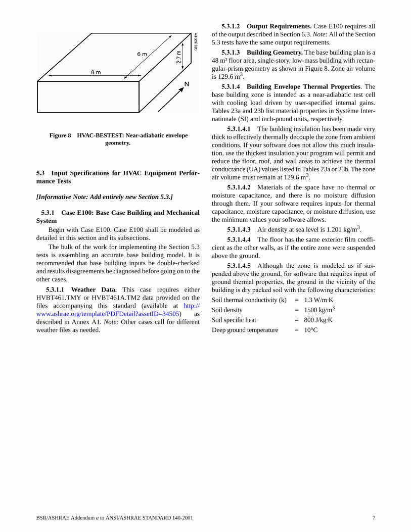
5.3.1.3 Building Geometry. The base building plan is a48 m² floor area, single-story, low-mass building with rectan-gular-prism geometry as shown in Figure 8. Zone air volumeis 129.6 m3.
5.3.1.4 Building Envelope Thermal Properties. Thebase building zone is intended as a near-adiabatic test cellwith cooling load driven by user-specified internal gains.Tables 23a and 23b list material properties in Système Inter-nationale (SI) and inch-pound units, respectively.
5.3.1.4.1 The building insulation has been made verythick to effectively thermally decouple the zone from ambientconditions. If your software does not allow this much insula-tion, use the thickest insulation your program will permit andreduce the floor, roof, and wall areas to achieve the thermalconductance (UA) values listed in Tables 23a or 23b. The zoneair volume must remain at 129.6 m3.
5.3.1.4.2 Materials of the space have no thermal ormoisture capacitance, and there is no moisture diffusionthrough them. If your software requires inputs for thermalcapacitance, moisture capacitance, or moisture diffusion, usethe minimum values your software allows.
5.3.1.4.3 Air density at sea level is 1.201 kg/m3.
5.3.1.4.4 The floor has the same exterior film coeffi-cient as the other walls, as if the entire zone were suspendedabove the ground.
5.3.1.4.5 Although the zone is modeled as if sus-
pended above the ground, for software that requires input of
ground thermal properties, the ground in the vicinity of the
building is dry packed soil with the following characteristics:
Soil thermal conductivity (k) = 1.3 W/m·K
Soil density = 1500 kg/m3
Soil specific heat = 800 J/kg·K
Deep ground temperature = 10°C
Figure 8 HVAC-BESTEST: Near-adiabatic envelope geometry.
BSR/ASHRAE Addendum a to ANSI/ASHRAE STANDARD 140-2001 7

8 BSR/ASHRAE Addendum a to ANSI/ASHRAE STANDARD 140-2001
TABLE 23a
Material Specifications Base Case (SI Units)
BSR/ASHRAE Addendum a to ANSI/ASHRAE STANDARD 140-2001 9
TABLE 23bMaterial Specifications Base Case (English Units)
5.3.1.5 Infiltration.
Infiltration rate = 0.0 ACH (air changes per hour) for the entire simulation period.
5.3.1.6 Internal Heat Gains.
Sensible internal gains = 5400 W (18430 Btu/h), continuously (24 hours per day for the full simulation period).
Latent internal gains = 0 W (0 Btu/h), continuously (24 hours per day for the full simulation period).
Sensible internal gains are 100% convective.Zone sensible and latent internal gains are assumed to be
distributed evenly throughout the zone air. These are internallygenerated sources of heat (from equipment, lights, people,etc.) that are not related to the operation of the mechanicalcooling system or its air distribution fan.
5.3.1.7 Opaque Surface Radiative Properties. Inte-rior and exterior opaque surface solar (visible and ultravioletwavelengths) absorptances and infrared emittances areincluded in Table 24.
5.3.1.8 Exterior Combined Radiative and ConvectiveSurface Coefficients. If the program being tested automati-cally calculates exterior surface radiation and convection, thissection may be disregarded. If the program being tested doesnot calculate this effect, then use 29.3 W/m²K for all exteriorsurfaces. This value is based on a mean annual wind speed of4.02 m/s for a surface with roughness equivalent to roughplaster or brick and is consistent with informative Annex B4.
5.3.1.9 Interior Combined Radiative and ConvectiveSurface Coefficients. If the program being tested automati-cally calculates interior surface radiation and convection, thenthis section can be disregarded. If the program being testeddoes not calculate these effects, then use the constant com-bined radiative and convective surface coefficients given inTable 25.
The radiative portion of these combined coefficients maybe taken as 5.13 W/m2K [0.90 Btu/(hft²F)] for an interiorinfrared emissivity of 0.9.
If the program being tested does not allow you to schedulethese coefficients, then use 8.29 W/m2K [1.46 Btu/(hft²F)] forall horizontal surfaces. If different values can be justified, thenuse different values.
Informative Annex B5 includes background informationabout combined radiative and convective film coefficients.
5.3.1.10 Mechanical System. The mechanical systemrepresents a simple vapor compression cooling system, ormore precisely, a unitary split air-conditioning system con-sisting of an air-cooled condensing unit and indoor evaporatorcoil. Figure 9 is a schematic diagram of this system. See Sec-tion 3 for definitions of terminology used in this section.
5.3.1.10.1 General Information.
• 100% convective air system• Zone air is perfectly mixed • No outside air; no exhaust air• Single-speed, draw-through air distribution fan • Indoor and outdoor fans cycle on and off together with
compressor• Air-cooled condenser
TABLE 24Opaque Surface Radiative Properties
Interior Surface Exterior Surface
Solar Absorptance 0.6 0.1
Infrared Emittance 0.9 0.9
TABLE 25
Interior Combined Surface Coefficient versus Surface Orientation
Orientation of Surface and Heat Flow Interior Combined Surface Coefficient
Horizontal heat transfer on vertical surfaces 8.29 W/m2K (1.46 Btu/(hft²F))
Upward heat transfer on horizontal surfaces 9.26 W/m2K (1.63 Btu/(hft²F))
Downward heat transfer on horizontal surfaces 6.13 W/m2K (1.08 Btu/(hft²F))
Figure 9 Unitary split air-conditioning system consisting of an air-cooled condensing unit and indoor evaporator coil.
10 BSR/ASHRAE Addendum a to ANSI/ASHRAE STANDARD 140-2001

• Single-speed reciprocating compressor, R-22 refriger-ant, no cylinder unloading
• No system hot gas bypass• The compressor, condenser, and condenser fan are
located outside the conditioned zone• All zone air moisture that condenses on the evaporator
coil (latent load) leaves the system through a condensatedrain
• Crankcase heater and other auxiliary energy = 0
Note that, in one of the field-trial simulations, simulta-neous use of “0” outside air and “0” infiltration caused an errorin the simulations. We worked around this by specifying mini-mum outside air = 0.000001 ft3/min. We recommend doing asensitivity test to check that using 0 for both these inputs doesnot cause a problem.
5.3.1.10.2 Thermostat Control Strategy.
Heat = off
Cool = on if zone air temperature > 22.2°C (72.0°F); other-wise cool = off.
There is no zone humidity control. This means that thezone humidity level will float in accordance with zone latentloads and moisture removal by the mechanical system.
The thermostat senses only the zone air temperature; thethermostat itself does not sense any radiant heat transferexchange with the interior surfaces.
The controls for this system are ideal in that the equip-ment is assumed to maintain the setpoint exactly when it isoperating and not overloaded. There are no minimum on or offtime-duration requirements for the unit and no hysteresiscontrol band (e.g., there is no ON at setpoint + x°C or OFF atsetpoint – y°C). If your software requires input for these, usethe minimum values your software allows.
The thermostat is nonproportional in the sense that whenthe conditioned zone air temperature exceeds the thermostatcooling setpoint, the heat extraction rate is assumed to equalthe maximum capacity of the cooling equipment correspond-ing to environmental conditions at the time of operation. Aproportional thermostat model can be made to approximate anonproportional thermostat model by setting a very smallthrottling range (the minimum allowed by your program). ACOP = f(PLR) curve is given in Section 5.3.1.10.4 to accountfor equipment cycling.
5.3.1.10.3 Full-Load Cooling System PerformanceData. Equipment full-load capacity and full-load perfor-mance data A-3 are given in six formats in Tables 26a through26f. Before using these tables, read all of the discussion in thissection (5.3.1.10.3) and its subsections (5.3.1.10.3.1 through5.3.1.10.3.6). Use the table that most closely matches the
input requirements of the software being tested. The tablescontain similar information with the following differences:
• Table 26a lists net capacities (SI units)• Table 26b lists net capacities (I-P units)• Table 26c lists gross capacities (SI units)• Table 26d lists gross capacities (I-P units)• Table 26e lists adjusted net capacities (SI units)• Table 26f lists adjusted net capacities (I-P units).
5.3.1.10.3.1 For convenience, an electronic file(PERFMAP140.XLS) that contains these tables is includedin the files accompanying this standard (available at http://www.ashrae.org/template/PDFDetail?assetID=34505).
5.3.1.10.3.2 The meaning of the various ways torepresent system capacity is discussed below; specific termsare also defined in Section 3. These tables use outdoor dry-bulb temperature (ODB), entering dry-bulb temperature(EDB), and entering wet-bulb temperature (EWB) as inde-pendent variables for performance data; the location of EDBand EWB is shown in Figure 9.
Listed capacities of Tables 26a and 26b are net valuesafter subtracting manufacturer default fan heat based on 365W per 1,000 cubic feet per minute (CFM), so the default fanheat for the 900 CFM fan is 329 W. For example, in Table 26athe listed net total capacity at Air-Conditioning and Refriger-ation Institute (ARI) rating conditions (EDB = 26.7°C,outdoor dry-bulb temperature [ODB] = 35.0°C, EWB =19.4°C) is 7852 W, and the assumed fan heat is 329 W. There-fore, the gross total capacity (see Table 26c) of the system atARI rating conditions—including both the net total capacityand the distribution system fan heat—is 7,852 + 329 = 8,181W. Similarly, the gross sensible capacity—including both thenet sensible capacity and air distribution system fan heat—is6,040 + 329 = 6,369 W.
The unit as described actually uses a 230 W fan. There-fore, the “real” net capacity is actually an adjusted net capac-ity, (net cap)adj, which is determined by
(net cap)adj = (net cap)listed + (default fan heat) – (actual fan power),
so for the adjusted net total (sensible + latent) capacity at ARIconditions and 900 CFM,
(net cap)adj = 7852 W + 329 W – 230 W = 7951 W.
The technique for determining adjusted net sensiblecapacities (see Table 26e) is similar.
5.3.1.10.3.3 Validity of Listed Data (VERYIMPORTANT). Compressor kW (kilowatts) and apparatusdew point, along with net total, gross total, and adjusted nettotal capacities given in Tables 26a through 26f, are valid
BSR/ASHRAE Addendum a to ANSI/ASHRAE STANDARD 140-2001 11
12 BSR/ASHRAE Addendum a to ANSI/ASHRAE STANDARD 140-2001
TABLE 26a
Equipment Full-Load Performance1 (SI Units)

BSR/ASHRAE Addendum a to ANSI/ASHRAE STANDARD 140-2001 13
TABLE 26b
Equipment Full-Load Performance1 (I-P Units)

14 BSR/ASHRAE Addendum a to ANSI/ASHRAE STANDARD 140-2001
TABLE 26c
Equipment Full-Load Performance with Gross Capacities1 (SI Units)
BSR/ASHRAE Addendum a to ANSI/ASHRAE STANDARD 140-2001 15
TABLE 26dEquipment Full-Load Performance with Gross Capacities1 (I-P Units)

16 BSR/ASHRAE Addendum a to ANSI/ASHRAE STANDARD 140-2001
TABLE 26eEquipment Full-Load Performance with Adjusted Net Capacities1 (SI Units)

BSR/ASHRAE Addendum a to ANSI/ASHRAE STANDARD 140-2001 17
TABLE 26fEquipment Full-Load Performance with Adjusted Net Capacities1 (I-P Units)
only for “wet” coils (when dehumidification is occurring). Adry-coil condition—no dehumidification—occurs when theentering air humidity ratio is decreased to the point wherethe entering air dew-point temperature is less than the effec-tive coil surface temperature (apparatus dew point). In Tables26a through 26f, the dry-coil condition is evident from agiven table for conditions where the listed sensible capacityis greater than the corresponding total capacity. For such adry-coil condition, set total capacity equal to sensible capac-ity.
For a given EDB and ODB, the compressor power, totalcapacity, sensible capacity, and apparatus dew point for wetcoils change only with varying EWB. Once the coil becomesdry—which is apparent for a given EDB and ODB from themaximum EWB where total and sensible capacities areequal— for a given EDB, compressor power and capacitiesremain constant with decreasing EWB.A-4
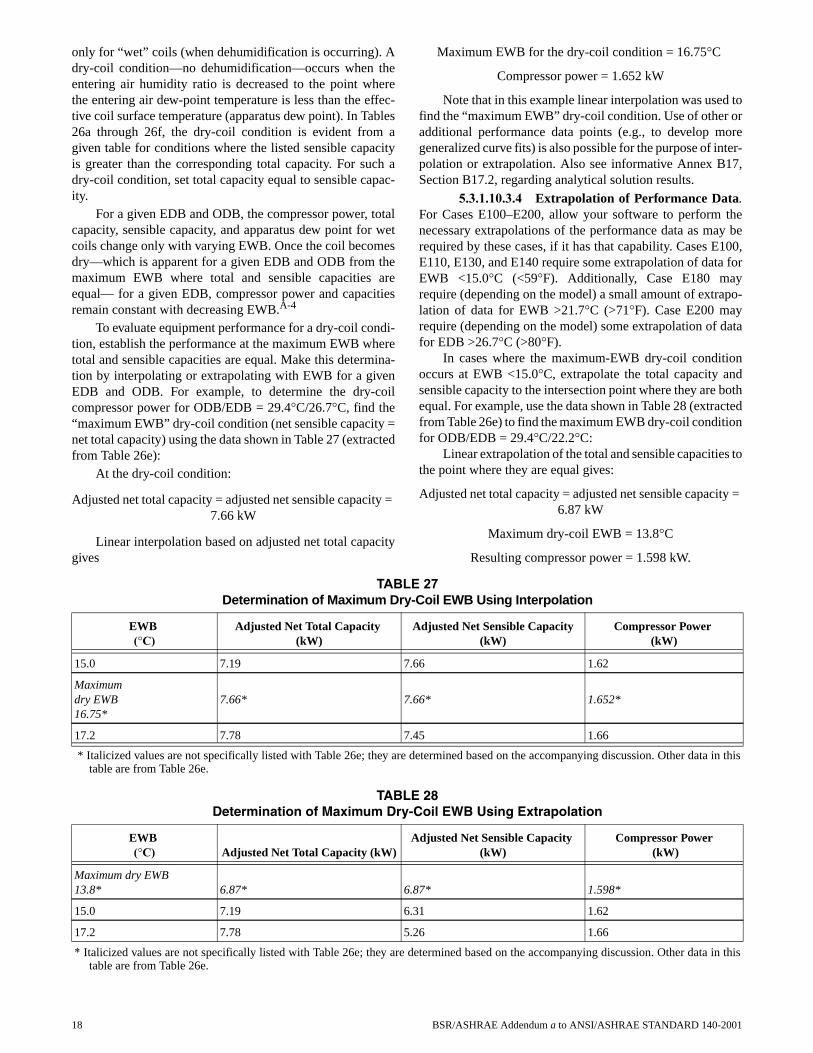
To evaluate equipment performance for a dry-coil condi-tion, establish the performance at the maximum EWB wheretotal and sensible capacities are equal. Make this determina-tion by interpolating or extrapolating with EWB for a givenEDB and ODB. For example, to determine the dry-coilcompressor power for ODB/EDB = 29.4°C/26.7°C, find the“maximum EWB” dry-coil condition (net sensible capacity =net total capacity) using the data shown in Table 27 (extractedfrom Table 26e):
At the dry-coil condition:
Adjusted net total capacity = adjusted net sensible capacity = 7.66 kW
Linear interpolation based on adjusted net total capacitygives
Maximum EWB for the dry-coil condition = 16.75°C
Compressor power = 1.652 kW
Note that in this example linear interpolation was used tofind the “maximum EWB” dry-coil condition. Use of other oradditional performance data points (e.g., to develop moregeneralized curve fits) is also possible for the purpose of inter-polation or extrapolation. Also see informative Annex B17,Section B17.2, regarding analytical solution results.
5.3.1.10.3.4 Extrapolation of Performance Data.For Cases E100–E200, allow your software to perform thenecessary extrapolations of the performance data as may berequired by these cases, if it has that capability. Cases E100,E110, E130, and E140 require some extrapolation of data forEWB <15.0°C (<59°F). Additionally, Case E180 mayrequire (depending on the model) a small amount of extrapo-lation of data for EWB >21.7°C (>71°F). Case E200 mayrequire (depending on the model) some extrapolation of datafor EDB >26.7°C (>80°F).
In cases where the maximum-EWB dry-coil conditionoccurs at EWB <15.0°C, extrapolate the total capacity andsensible capacity to the intersection point where they are bothequal. For example, use the data shown in Table 28 (extractedfrom Table 26e) to find the maximum EWB dry-coil conditionfor ODB/EDB = 29.4°C/22.2°C:
Linear extrapolation of the total and sensible capacities tothe point where they are equal gives:
Adjusted net total capacity = adjusted net sensible capacity = 6.87 kW
Maximum dry-coil EWB = 13.8°C
Resulting compressor power = 1.598 kW.
TABLE 27
Determination of Maximum Dry-Coil EWB Using Interpolation
EWB (°C)
Adjusted Net Total Capacity (kW)
Adjusted Net Sensible Capacity (kW)
Compressor Power (kW)
15.0 7.19 7.66 1.62
Maximumdry EWB16.75*
7.66* 7.66* 1.652*
17.2 7.78 7.45 1.66
* Italicized values are not specifically listed with Table 26e; they are determined based on the accompanying discussion. Other data in thistable are from Table 26e.
TABLE 28Determination of Maximum Dry-Coil EWB Using Extrapolation
EWB (°C) Adjusted Net Total Capacity (kW)
Adjusted Net Sensible Capacity (kW)
Compressor Power (kW)
Maximum dry EWB13.8* 6.87* 6.87* 1.598*
15.0 7.19 6.31 1.62
17.2 7.78 5.26 1.66
* Italicized values are not specifically listed with Table 26e; they are determined based on the accompanying discussion. Other data in thistable are from Table 26e.
18 BSR/ASHRAE Addendum a to ANSI/ASHRAE STANDARD 140-2001

Note that in this example linear extrapolation was used tofind the “maximum EWB” dry-coil condition. Use of other oradditional performance data points (e.g., to develop moregeneralized curve fits) is also possible for the purpose of inter-polation or extrapolation. Also see informative Annex B17,Section B17.2, regarding analytical solution results.
5.3.1.10.3.5 Apparatus Dew Point. Apparatusdew point (ADP) is defined in Section 3. Listed values ofADP may vary somewhat from those calculated using theother listed performance parameters. For more discussion ofthis, see informative Annex B14 (Cooling Coil Bypass Fac-tor).
5.3.1.10.3.6 Values at ARI Rating Conditions. InTables 26a through 26f, nominal values at ARI rating condi-tions are useful to system designers for comparing the capa-bilities of one system to those of another. Some detailedsimulation programs utilize inputs for ARI rating conditionsin conjunction with the full performance maps of Tables 26athrough 26f. For simplified simulation programs and otherprograms that do not allow performance maps of certainparameters, appropriate values at ARI conditions may beused and assumed constant.
5.3.1.10.3.7 SEER. In Tables 26a through 26f, sea-sonal energy efficiency ratio (SEER), which is a generalizedseasonal efficiency rating, is not generally a useful input fordetailed simulation of mechanical systems. SEER (or“COPSEER” in the metric versions) is useful to systemdesigners for comparing one system to another. SEER is fur-ther discussed in Section 3 and informative Annex B13.
5.3.1.10.3.8 Cooling Coil Bypass Factor. If yoursoftware does not require an input for bypass factor (BF) orautomatically calculates it based on other inputs, ignore thisinformation.
BF at ARI rating conditions is approximately 0.049 ≤ BF≤ 0.080.
Calculation techniques and uncertainty about this rangeof values are discussed in informative Annex B14. Annex B14is provided for illustrative purposes; some models mayperform the calculation with minor differences in technique orassumptions or both. If your software requires this input,calculate the BF in a manner consistent with the assumptionsof your specific model. If the assumptions of your model arenot apparent from its documentation, use a value consistentwith the above range and Annex B14.
Calculations based on the listed performance data indi-cate that BF varies as a function of EDB, EWB, and ODB.Incorporate this aspect of equipment performance into yourmodel if your software allows it, using a consistent method fordeveloping all points of the BF variation map.
5.3.1.10.3.9 Minimum Supply Air Temperature.This system is a variable temperature system, meaning thatthe supply air temperature varies with the operating condi-tions. If your software requires an input for minimum allow-able supply air temperature, use
Minimum supply air temperature ≤ 7.7°C (45.9°F).
This value is the lowest value of ADP that occurs in theSection 5.3 test cases based on the quasi-analytical solutionsfor Case E110 presented in HVAC BESTEST.A-5
If your software does not require this input, ignore thisinformation.
5.3.1.10.4 Part-Load Operation. The system COPdegradation that results from part-load operation is describedin Figure 10. In this figure the COP degradation factor (CDF)is a multiplier to be applied to the full-load system COP (asdefined in Section 3) at a given part-load ratio (PLR), where
COP(PLR) = (full load COP(ODB,EWB,EDB)) * CDF(PLR).
This representation is based on information provided bythe equipment manufacturer. It might be helpful to think of theefficiency degradation as being caused by additional start-uprun time required to bring the evaporator coil temperaturedown to its equilibrium temperature for the time(s) when thecompressor is required to operate during an hour with partload. Then, because the controller is ideal ON/OFF cycling(see Section 5.3.1.10.2),
Hourly fractional run time = PLR/CDF.
In Figure 10, the PLR is calculated by
(Net refrigeration effect) / (Adjusted net total capacity) ,
where the net refrigeration effect and the adjusted net totalcapacity are as defined in Section 3.
PLR may be alternatively calculated as
(Gross total coil load) / (Gross total capacity) ,
where the gross total coil load and gross total capacity are asdefined in Section 3. Demonstration of the similarity of thesedefinitions of PLR is included in Annex B13, Section B13.2.
Simplifying assumptions in Figure 10 are:
• There is no minimum on/off time for the compressorand related fans; they may cycle on/off as often as nec-essary to maintain the setpoint.
• The decrease in efficiency with increased on/off cyclingat very low PLR remains linear.
Figure 10 Cooling equipment part load performance (COP degradation factor versus PLR).
BSR/ASHRAE Addendum a to ANSI/ASHRAE STANDARD 140-2001 19
Annex B13 includes additional details about how Figure10 was derived.
If your software utilizes the cooling coil bypass factor,model the BF as independent of (not varying with) the PLR.
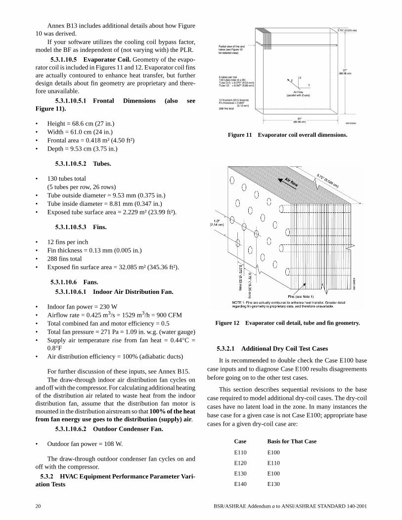
5.3.1.10.5 Evaporator Coil. Geometry of the evapo-rator coil is included in Figures 11 and 12. Evaporator coil finsare actually contoured to enhance heat transfer, but furtherdesign details about fin geometry are proprietary and there-fore unavailable.
5.3.1.10.5.1 Frontal Dimensions (also seeFigure 11).
• Height = 68.6 cm (27 in.)• Width = 61.0 cm (24 in.)• Frontal area = 0.418 m² (4.50 ft²)• Depth = 9.53 cm (3.75 in.)
5.3.1.10.5.2 Tubes.
• 130 tubes total(5 tubes per row, 26 rows)
• Tube outside diameter = 9.53 mm (0.375 in.) • Tube inside diameter = 8.81 mm (0.347 in.)• Exposed tube surface area = 2.229 m² (23.99 ft²).
5.3.1.10.5.3 Fins.
• 12 fins per inch• Fin thickness = 0.13 mm (0.005 in.)• 288 fins total• Exposed fin surface area = 32.085 m² (345.36 ft²).
5.3.1.10.6 Fans.
5.3.1.10.6.1 Indoor Air Distribution Fan.
• Indoor fan power = 230 W• Airflow rate = 0.425 m3/s = 1529 m3/h = 900 CFM• Total combined fan and motor efficiency = 0.5• Total fan pressure = 271 Pa = 1.09 in. w.g. (water gauge)• Supply air temperature rise from fan heat = 0.44°C =
0.8°F• Air distribution efficiency = 100% (adiabatic ducts)
For further discussion of these inputs, see Annex B15.The draw-through indoor air distribution fan cycles on
and off with the compressor. For calculating additional heatingof the distribution air related to waste heat from the indoordistribution fan, assume that the distribution fan motor ismounted in the distribution airstream so that 100% of the heatfrom fan energy use goes to the distribution (supply) air.
5.3.1.10.6.2 Outdoor Condenser Fan.
• Outdoor fan power = 108 W.
The draw-through outdoor condenser fan cycles on andoff with the compressor.
5.3.2 HVAC Equipment Performance Parameter Vari-ation Tests
5.3.2.1 Additional Dry Coil Test Cases
It is recommended to double check the Case E100 basecase inputs and to diagnose Case E100 results disagreementsbefore going on to the other test cases.
This section describes sequential revisions to the basecase required to model additional dry-coil cases. The dry-coilcases have no latent load in the zone. In many instances thebase case for a given case is not Case E100; appropriate basecases for a given dry-coil case are:
Case Basis for That Case
E110 E100
E120 E110
E130 E100
E140 E130
Figure 11 Evaporator coil overall dimensions.
Figure 12 Evaporator coil detail, tube and fin geometry.
20 BSR/ASHRAE Addendum a to ANSI/ASHRAE STANDARD 140-2001
5.3.2.1.1 Case E110: Reduced Outdoor Dry-BulbTemperature. Case E110 is exactly the same as Case E100except the applicable weather data file is
HVBT294.TMY or HVBT294A.TM2.
These data are provided in the files accompanying thisstandard (available at http://www.ashrae.org/template/PDFDetail?assetID=34505) as described in Annex A1,Section A1.2.
5.3.2.1.2 Case E120: Increased Thermostat Set-point. Case E120 is exactly the same as Case E110 except thethermostat control strategy is:
Heat = off
Cool = on if zone air temperature >26.7°C (80.0°F); otherwise cool = off
All other features of the thermostat remain as before.
5.3.2.1.3 Case E130: Low Part-Load Ratio. CaseE130 is exactly the same as Case E100 except the internal heatgains are:
Sensible internal gains = 270 W (922 Btu/h), continuously (24 hours per day for the full simulation period)
Latent internal gains = 0 W (0 Btu/h), continuously (24 hours per day for the full simulation period)
Sensible internal gains remain as 100% convective.Zone sensible internal gains are assumed to be distributed
evenly throughout the zone air. These are internally generatedsources of heat (from equipment, lights, people, etc.) that arenot related to the operation of the mechanical cooling systemor its air distribution fan.
5.3.2.1.4 Case E140: Reduced Outdoor Dry-BulbTemperature at Low Part-Load Ratio. Case E140 is exactlythe same as Case E130 except the weather applicable weatherdata file is
HVBT294.TMY or HVBT294A.TM2.
These data are provided in the files accompanying thisstandard as described in Annex A1, Section A1.2.
5.3.2.2 Humid Zone Test Cases. In this section, thesequential revisions required to model humid zone cases aredescribed. The humid zone cases have latent load in the zoneand, therefore, have moisture removed by the evaporator coil.All condensed moisture is assumed to leave the systemthrough a condensate drain. The appropriate base cases for agiven case are:
5.3.2.2.1 Case E150: Latent Load at High SensibleHeat Ratio. Case E150 is exactly as Case E110 except theinternal heat gains are:
Sensible internal gains = 5400 W (18430 Btu/h), continuously (24 hours per day for the full simulation period)
Latent internal gains = 1100 W (3754 Btu/h), continuously (24 hours per day for the full simulation period)
Sensible gains remain as 100% convective.Zone sensible and latent internal gains are assumed to be
distributed evenly throughout the zone air. These are internallygenerated sources of heat (from equipment, lights, people,etc.) that are not related to operation of the mechanical coolingsystem or its air distribution fan.
If the software being tested requires input of water vapormass flow rate rather than latent internal gains, then to convertthe listed latent internal gains to water vapor mass flow rate,use a heat of vaporization (hfg) that approximates the value ofhfg for condensation at the coil used by the software beingtested.
If the software being tested requires input of total internalgains, then use the sum of listed sensible + latent internalgains.
5.3.2.2.2 Case E160: Increased Thermostat Set-point at High Sensible Heat Ratio. Case E160 is exactly thesame as Case E150 except the thermostat control strategy is:
Heat = off
Cool = on if zone air temperature >26.7°C (80.0°F); otherwise cool = off
All other features of the thermostat remain as before.
5.3.2.2.3 Case E165: Variation of Thermostat Set-point and Outdoor Dry-Bulb Temperature at High Sensi-ble Heat Ratio. Case E165 is exactly the same as Case E160except the thermostat control strategy and weather data arechanged as noted below.
5.3.2.2.3.1 Weather Data
HVBT406.TMY or HVBT406A.TM2
These data are provided in the files accompanying thisstandard as described in Annex A1, Section A1.2.
5.3.2.2.3.2 Thermostat control strategy
Heat = off
Cool = on if zone air temperature >23.3°C (74.0°F); otherwise cool = off
All other features of the thermostat remain as before.
5.3.2.2.4 Case E170: Reduced Sensible Load. CaseE170 is exactly the same as Case E150 except the internal heatgains are:
Sensible internal gains = 2100 W (7166 Btu/h), continuously (24 hours per day for the full simulation period)
Latent internal gains = 1100 W (3754 Btu/h), continuously (24 hours per day for the full simulation period)
Sensible gains remain as 100% convective.
Case Basis for That Case
E150 E110
E160 E150
E165 E160
E170 E150
E180 E170
E185 E180
E190 E180
E195 E190
E200 E150
BSR/ASHRAE Addendum a to ANSI/ASHRAE STANDARD 140-2001 21

Zone sensible and latent internal gains are assumed to bedistributed evenly throughout the zone air. These are internallygenerated sources of heat (from equipment, lights, people,etc.) that are not related to operation of the mechanical coolingsystem or its air distribution fan.
If the software being tested requires input of water vapormass flow rate rather than latent internal gains, then to convertthe listed latent internal gains to water vapor mass flow rate,use a heat of vaporization (hfg) that approximates the value ofhfg for condensation at the coil used by the software beingtested.
If the software being tested requires input of total internalgains, then use the sum of listed sensible + latent internalgains.
5.3.2.2.5 Case E180: Increased Latent Load. CaseE180 is exactly the same as Case E170 except the internal heatgains are:
Sensible internal gains = 2100 W (7166 Btu/h), continuously (24 hours per day for the full simulation period)
Latent internal gains = 4400 W (15018 Btu/h), continuously (24 hours per day for the full simulation period).
Sensible gains remain as 100% convective.Zone sensible and latent internal gains are assumed to be
distributed evenly throughout the zone air. These are internallygenerated sources of heat (from equipment, lights, people,etc.) that are not related to operation of the mechanical coolingsystem or its air distribution fan.
If the software being tested requires input of water vapormass flow rate rather than latent internal gains, then to convertthe listed latent internal gains to water vapor mass flow rate,use a heat of vaporization (hfg) that approximates the value ofhfg for condensation at the coil used by the software beingtested.
If the software being tested requires input of total internalgains, then use the sum of listed sensible + latent internalgains.
5.3.2.2.6 Case E185: Increased Outdoor Dry-BulbTemperature at Low Sensible Heat Ratio. Case E185 isexactly the same as Case E180 except the weather applicableweather data file is
HVBT461.TMY or HVBT461A.TM2.
These data are provided in the files accompanying this stan-dard (available at http://www.ashrae.org/template/PDFDe-tail?assetID=34505) as described in Annex A1, Section A1.2.
5.3.2.2.7 Case E190: Low Part-Load Ratio at LowSensible Heat Ratio. Case E190 is exactly the same as CaseE180 except the internal heat gains are:
Sensible internal gains = 270 W (922 Btu/h), continuously (24 hours per day for the full simulation period)
Latent internal gains = 550 W (1877 Btu/h), continuously (24 hours per day for the full simulation period)
Sensible gains remain as 100% convective.Zone sensible and latent internal gains are assumed to be
distributed evenly throughout the zone air. These are internallygenerated sources of heat (from equipment, lights, people,
etc.) that are not related to operation of the mechanical coolingsystem or its air distribution fan.
If the software being tested requires input of water vapormass flow rate rather than latent internal gains, then to convertthe listed latent internal gains to water vapor mass flow rate,use a heat of vaporization (hfg) that approximates the value ofhfg for condensation at the coil used by the software beingtested.
If the software being tested requires input of total internalgains, then use the sum of listed sensible + latent internalgains.
5.3.2.2.8 Case E195: Increased Outdoor Dry-BulbTemperature at Low Sensible Heat Ratio and Low Part-Load Ratio. Case E195 is exactly the same as Case E190except the weather applicable weather data file is
HVBT461.TMY or HVBT461A.TM2.
These data are provided in the files accompanying this stan-dard as described in Annex A1, Section A1.2.
5.3.2.2.9 Case E200: Full-Load Test at ARI Condi-tions. This case compares simulated performance of mechan-ical equipment to the manufacturer’s listed performance atfull load and at ARI-specified operating conditions. CaseE200 is exactly the same as Case E150 except for the changesnoted below.
5.3.2.2.9.1 Weather Data
HVBT350.TMY or HVBT350A.TM2.
These data are provided in the files accompanying this stan-dard as described in Annex A1, Section A1.2.
5.3.2.2.9.2 Internal heat gains
Sensible internal gains = 6120 W (20890 Btu/h), continuously (24 hours per day for the full simulation period)
Latent internal gains = 1817 W (6200 Btu/h), continuously (24 hours per day for the full simulation period).
Sensible gains remain as 100% convective.Zone sensible and latent internal gains are assumed to be
distributed evenly throughout the zone air. These are internallygenerated sources of heat (from equipment, lights, people,etc.) that are not related to operation of the mechanical coolingsystem or its air distribution fan.
If the software being tested requires input of water vapormass flow rate rather than latent internal gains, then to convertthe listed latent internal gains to water vapor mass flow rate,use a heat of vaporization (hfg) that approximates the value ofhfg for condensation at the coil used by the software beingtested.
If the software being tested requires input of total internalgains, then use the sum of listed sensible + latent internalgains.
5.3.2.2.9.3 Thermostat Control Strategy
Heat = off.
Cool = on if zone air temperature > 26.7°C (80.0°F); other-wise cool = off.
All other features of the thermostat remain as before.
22 BSR/ASHRAE Addendum a to ANSI/ASHRAE STANDARD 140-2001

6. OUTPUT REQUIREMENTS
[Informative Note: Make the following revisions to Section6.]
6.1 Annual Outputs for Building Thermal Envelope andFabric Load Tests of Section 5.2
6.1.1 All Non-Free-Float Cases. In this description, theterm “free-float cases” refers to cases designated with FF inthe case description (i.e., 600FF, 650FF, 900FF, 950FF); non-free-float cases are all the other cases described in Section 5.2(Annex B1 includes an informative summary listing of all thecases). Required outputs for the non-free-float cases are:
6.1.1.5 All heating and cooling loads listed in 6.1.1.1
through 6.1.1.4 shall be entered into the appropriate standard
output report (see Annex A2) as positive values (≥0).
6.2 Daily Hourly Output for Building Thermal Envelopeand Fabric Load Tests of Section 5.2
If the program being tested can produce hourly outputs,then produce the following hourly values for the specifieddays. To produce this output, run the program for a normalannual run. Do not just run the required days because theresults could contain temperature history errors. Requiredoutputs are listed for specific cases in Table 293.
Table 293Daily Hourly Output Requirements for Building Thermal
Envelope and Fabric Load Tests of Section 5.2
6.3 Output Requirements for HVAC Equipment Perfor-mance Tests of Section 5.3
6.3.1 The outputs listed immediately below are to includeloads or consumptions (as appropriate) for the entire month ofFebruary (the second month in the weather data sets). Theterms cooling energy consumption, evaporator coil loads,zone cooling loads, and coefficient of performance are definedin Section 3.
6.3.1.1 Cooling energy consumptions (kWh) (a) Total consumption (compressor and fans)(b) Disaggregated compressor consumption(c) Disaggregated indoor air distribution fan consumption(d) Disaggregated outdoor condenser fan consumption
6.3.1.2 Evaporator coil loads (kWh)(a) Total evaporator coil load (sensible + latent)(b) Disaggregated sensible evaporator coil load(c) Disaggregated latent evaporator coil load
6.3.1.3 Zone cooling loads (kWh)(a) Total cooling load (sensible + latent)(b) Disaggregated sensible cooling load(c) Disaggregated latent cooling load.
6.3.2 The outputs listed immediately below are to includethe mean value for the month of February and the hourly inte-grated maximum and minimum values for the month of Feb-ruary. (a) Calculated coefficient of performance (COP) (dimension-
less)
((Net refrigeration effect)/(total cooling energy consump-tion))
(b) Zone dry- bulb temperature (°C)(c) Zone humidity ratio (kg moisture/kg dry air).
(This is a normative annex and is part of the standard.)
ANNEX A1
WEATHER DATA[Informative Note: Create new Section A1.1 by combiningthe first paragraph of Annex A1 and the first sentence of thesecond paragraph and revising as follows.]
A1.1 Weather Data for Building Thermal Envelope andFabric Load Tests
The full-year weather data (DRYCOLD.TMY) in the filesaccompanying this standard method of test (available at http://www.ashrae.org/template/PDFDetail?assetID=34505) shallbe used for performing the tests called out in Section 5.2. Siteand weather characteristics are summarized in Table A1-1.
A1.2 Weather Data for HVAC Equipment PerformanceTests
The weather data listed in Table A1-2 shall be used ascalled out in Section 5.3. These data files represent TMY andTMY2 format weather data files, respectively, with modifica-tions so that the initial fundamental series of mechanicalequipment tests may be very tightly controlled. The TMY-format data are three-month-long data files used in the originalfield trials of the test procedure; the TMY2-format data areyear-long data files that may be more convenient for users. Forthe purposes of HVAC BESTEST, which uses a near-adiabaticbuilding envelope, the TMY and TMY2 data sets are equiva-lent. (Note that there are small differences in solar radiation,wind speed, etc., that result in a sensible loads difference of0.2%-0.3% in cases with low internal gains [i.e., E130, E140,E190, and E195]. This percentage load difference is less[0.01%-0.04%] for the other cases because they have higherinternal gains. These TMY and TMY2 data are not equivalentfor use with a non-near-adiabatic building envelope.)
Ambient dry-bulb and dew-point temperatures areconstant in all the weather files; constant values of ambientdry-bulb temperature vary among the files according to the filename. Site and weather characteristics are summarized inTables A1-3a and A1-3b for the TMY and TMY2 data files,respectively. Details about the TMY and TMY2 weather datafile formats are included in Sections A1.3 and A1.4 respec-tively.
[Informative Note: Revise the title of Table A1-1 as follows.]
TABLE A1-1
Site and Weather Summary for DRYCOLD.TMY Weather Data Used with Building Thermal Envelope
and Fabric Load Tests
BSR/ASHRAE Addendum a to ANSI/ASHRAE STANDARD 140-2001 23
[Informative Note: Add entirely new Tables A1-2, A1-3a, and A1-3b as noted.]
TABLE A1-2Weather Data for HVAC Equipment Performance Tests
Data Files Applicable Cases Applicable Cases’ Sections
HVBT294.TMY or HVBT294A.TM2 E110, E120, E140, E150, E160, E170, E180, E190
5.3.2.1.1; 5.3.2.1.2; 5.3.2.1.4; 5.3.2.2.1; 5.3.2.2.2; 5.3.2.2.4; 5.3.2.2.5; 5.3.2.2.7
HVBT350.TMY or HVBT350A.TM2 E200 5.3.2.2.9
HVBT406.TMY or HVBT406A.TM2 E165 5.3.2.2.3
HVBT461.TMY or HVBT461A.TM2 E100, E130, E185, E195 5.3.1; 5.3.2.1.3; 5.3.2.2.6; 5.3.2.2.8
TABLE A1-3aSite and Weather Summary for HVAC Equipment Performance Tests—TMY Data
Weather Type Artificial Conditions
Weather Format TMY
Latitude 25.8° North
Longitude (local site) 80.3° West
Altitude 2 m (6.6 ft)
Time Zone (Standard Meridian Longitude) 5 (75° West)
Ground Reflectivity 0.2
Site Flat, unobstructed, located exactly at weather station
Dew Point Temperature (constant) 14.0°C (57.2°F)
Humidity Ratio 0.010 kg moisture/kg dry air(0.010 lb moisture/lb dry air)
Mean 3-Month Wind Speed 4.4 m/s (9.8 miles/h)
Maximum 3-Month Wind Speed 12.4 m/s (27.7 miles/h)
Global Horizontal Solar Radiation 3-Month Total 1354 MJ/m² (119.2 kBtu/ft²)
Direct Normal Solar Radiation 3-Month Total 1350 MJ/m² (118.8 kBtu/ft²)
Direct Horizontal Solar Radiation 3-Month Total 817 MJ/m² (71.9 kBtu/ft²)
Diffuse Horizontal Solar Radiation 3-Month Total 536 MJ/m² (47.2 kBtu/ft²)
Quantities That Vary Between Data Sets Ambient Dry BulbTemperature (constant)
AmbientRelative Humidity
HVBT294.TMY 29.4°C (85.0°F) 39%
HVBT350.TMY 35.0°C (95.0°F) 28%
HVBT406.TMY 40.6°C (105.0°F) 21%
HVBT461.TMY 46.1°C (115.0°F) 16%
24 BSR/ASHRAE Addendum a to ANSI/ASHRAE STANDARD 140-2001
[Informative Note: Revise Section A1.3 as follows.]
A1.3 TMY Weather Data FormatFor those programs that do not have Typical Meteorolog-
ical Year (TMY) weather processors, TMY weather data fileformat is provided in Table A1-42. This reprint of tables alsoincludes some additional notes based on experience withTMY data. If this summary is insufficient, the complete docu-mentation on TMY weather data8 can be obtained from theNational Climatic Data Center (NCDC) in Asheville, NorthCarolina. The address is Federal Building, Asheville, NC28801-2733; telephone 828-271-4800. Informative Annex B2contains additional background information regarding TMYweather data.
The hourly time convention for TMY weather data issolar time, where
Solar Time = Standard Time + (4 minutes / degree) x (Lst - Lloc) + E
and where
Lst ≡ standard meridian longitude (degrees)
Lloc ≡ local site longitude (degrees)
E = 9.87 sin 2B - 7.53 cos B - 1.5 sin B229.2(0.000075 + 0.001868 cos(B) – 0.032077 sin(B) – 0.014615 cos(2B) –
0.04089 sin(2B) (minutes)
where
B = 360(n - 81)/364365 (degrees)
n ≡ day of the year, 1 ≤ n ≤ 365
E varies roughly ± 15 minutes throughout the yearbecause of cosmology. Additional background information onthe equation of time may be found in the references.4
Additional background regarding the difference betweensolar time and standard time is included in informative AnnexB11 (Section B11.3).
[Informative Note: Add entirely new Section A1.4 as below.]
A1.4 TMY2 Weather Data Format
For those programs that do not have Typical Meteorolog-ical Year 2 (TMY2) weather processors, TMY2 weather datafile format is described below. If this summary is insufficient,the complete documentation on TMY2 weather dataA-6 can beobtained at http://rredc.nrel.gov/solar/pubs/tmy2.
A1.4.1 File Header. The first record of each file is the fileheader that describes the station. The file header contains theWBAN number, city, state, time zone, latitude, longitude, andelevation. The field positions and definitions of these headerelements are given in Table A1-5, along with sample FOR-TRAN and C formats for reading the header. A sample of afile header and data for January 1 is shown in Figure A1-1.
A1.4.2 Hourly Records. Following the file header, 8,760hourly data records provide one year of solar radiation, illu-minance, and meteorological data, along with their source and
TABLE A1-3bSite and Weather Summary for HVAC Equipment Performance Tests—TMY2 Data
Weather Type Artificial Conditions
Weather Format TMY2
Latitude 25.8° North
Longitude (local site) 80.3° West
Altitude 2 m (6.6 ft)
Time Zone (Standard Meridian Longitude) 5 (75° West)
Ground Reflectivity 0.2
Site Flat, unobstructed, located exactly at weather station
Dew Point Temperature (constant) 14.0°C (57.2°F)
Humidity Ratio 0.010 kg moisture/kg dry air(0.010 lb moisture/lb dry air)
Mean Annual Wind Speed 4.3 m/s (9.7 miles/h)
Maximum Annual Wind Speed 13.9 m/s (31.1 miles/h)
Global Horizontal Solar Radiation Annual Total 6453 MJ/m² (568 kBtu/ft²)
Direct Normal Solar Radiation Annual Total 5418 MJ/m² (477 kBtu/ft²)
Diffuse Horizontal Solar Radiation Annual Total 2914 MJ/m² (257 kBtu/ft²)
Quantities That Vary Between Data Sets Ambient Dry BulbTemperature (constant)
AmbientRelative Humidity
HVBT294A.TM2 29.4°C (85.0°F) 39%
HVBT350A.TM2 35.0°C (95.0°F) 28%
HVBT406A.TM2 40.6°C (105.0°F) 21%
HVBT461A.TM2 46.1°C (115.0°F) 16%
BSR/ASHRAE Addendum a to ANSI/ASHRAE STANDARD 140-2001 25

uncertainty flags. Table A1-6 provides field positions, ele-ment definitions, and sample FORTRAN and C formats forreading the hourly records.
Each hourly record begins with the year (field positions 2-3) from which the typical month was chosen, followed by themonth, day, and hour information in field positions 4-9. Thetimes are in local standard time (previous TMYs based onSOLMET/ERSATZ data are in solar time).
For solar radiation and illuminance elements, the datavalues represent the energy received during the 60 minutespreceding the hour indicated. For meteorological elements(with a few exceptions), observations or measurements were
made at the hour indicated. A few of the meteorologicalelements had observations, measurements, or estimates madeat daily, instead of hourly, intervals. Consequently, the datavalues for broadband aerosol optical depth, snow depth, anddays since last snowfall represent the values available for theday indicated.
[Informative Note: Add Figure A1-1. Change the designa-tion of Table A1-2, Typical Meteorological Year DataFormat, to Table A1-4 on all pages on which the tableappears. Add tables A1-5 and A1-6.]
26 BSR/ASHRAE Addendum a to ANSI/ASHRAE STANDARD 140-2001
BSR/ASHRAE Addendum a to ANSI/ASHRAE STANDARD 140-2001 27
14944 SIOUX_FALLS SD -6 N 43 34 W 96 44 435
85010101000000000000?00000?00000?00000?00000?00000?00000?010A710A7-150A7-211A7060A70975A7360A7052A70161A700945A70999099999004E7050F8000A700E7
85010102000000000000?00000?00000?00000?00000?00000?00000?010A710A7-144A7-206A7060A70975A7350A7077A70161A700914A70999099999004E7050F8000A700E7
85010103000000000000?00000?00000?00000?00000?00000?00000?010A710A7-144A7-200A7063A70975A7340A7062A70161A700732A70999099999004E7050F8000A700E7
85010104000000000000?00000?00000?00000?00000?00000?00000?010A710A7-150A7-206A7063A70976A7330A7072A70161A700640A70999099999004E7050F8000A700E7
85010105000000000000?00000?00000?00000?00000?00000?00000?010A710A7-156A7-217A7060A70976A7330A7067A70161A700640A70999099999003E7050F8000A700E7
85010106000000000000?00000?00000?00000?00000?00000?00000?010A710A7-167A7-222A7062A70976A7340A7067A70161A700640A70999099999003E7050F8000A700E7
85010107000000000000?00000?00000?00000?00000?00000?00000?004A704A7-183A7-233A7065A70977A7300A7052A70193A777777A70999999999003E7050F8000A700E7
85010108000000000000?00000?00000?00000?00000?00000?00000?002A702A7-194A7-244A7065A70978A7310A7036A70193A777777A70999999999003E7050F8000A700E7
85010109010212970037G50173G40024G50038I50071I40033I50043I604A700A7-200A7-256A7062A70978A7330A7046A70193A777777A70999999999003E7050F8000A700E7
85010110028714150157G50560G40043G50159I50444I40069I50079I600A700A7-189A7-256A7056A70979A7310A7067A70193A777777A70999999999003E7050F8000A700E7
85010111043614150276G40714G40056G50286I40642I40088I50111I500A700A7-172A7-250A7051A70979A7310A7062A70161A777777A70999999999003E7050F8000A700E7
85010112053014150357G40782G40064G50374I40735I40098I50131I500A700A7-167A7-244A7051A70978A7300A7062A70161A777777A70999999999003E7050F8000A700E7
85010113056214150387G40806G40067G50407I40767I40101I50139I500A700A7-156A7-244A7047A70978A7320A7067A70193A777777A70999999999003E7050F8000A700E7
85010114053014150359G40788G40064G50377I40742I40098I50131I500A700A7-144A7-239A7045A70978A7310A7062A70193A777777A70999999999003E7050F8000A700E7
85010115043614150277G40716G40056G50289I40645I40088I50111I500A700A7-139A7-239A7043A70978A7330A7052A70193A777777A70999999999003E7050F8000A700E7
85010116028614150157G50564G40043G50162I50450I40069I50080I600A700A7-139A7-233A7045A70978A7300A7052A70161A777777A70999999999003E7050F8000A700E7
85010117010412730038G50209G40021G50038I50104I40030I50038I600A700A7-150A7-233A7049A70978A7290A7041A70241A777777A70999999999003E7050F8000A700E7
85010118000000000000?00000?00000?00000?00000?00000?00000?000A700A7-167A7-233A7057A70978A7000A7000A70241A777777A70999999999003E7050F8000A700E7
85010119000000000000?00000?00000?00000?00000?00000?00000?000A700A7-172A7-233A7059A70978A7000A7000A70241A777777A70999999999003E7050F8000A700E7
85010120000000000000?00000?00000?00000?00000?00000?00000?000A700A7-178A7-233A7062A70978A7000A7000A70241A777777A70999999999003E7050F8000A700E7
85010121000000000000?00000?00000?00000?00000?00000?00000?000A700A7-183A7-239A7062A70978A7260A7015A70241A777777A70999999999003E7050F8000A700E7
85010122000000000000?00000?00000?00000?00000?00000?00000?000A700A7-183A7-239A7062A70977A7220A7021A70241A777777A70999999999003E7050F8000A700E7
85010123000000000000?00000?00000?00000?00000?00000?00000?000A700A7-178A7-239A7059A70977A7220A7015A70241A777777A70999999999003E7050F8000A700E7
85010124000000000000?00000?00000?00000?00000?00000?00000?000A700A7-178A7-239A7059A70977A7240A7010A70241A777777A70999999999003E7050F8000A700E7
1 1 1 1 1
1 2 3 4 5 6 7 8 9 0 1 2 3 4
1234567890123456789012345678901234567890123456789012345678901234567890123456789012345678901234567890123456789012345678901234567890123456789012
(for field position identification only)
Fig
ure
A1-
1Sa
mpl
e fi
le h
eade
r an
d da
ta in
the
TM
Y2
form
at fo
r Ja
nuar
y 1
TABLE A1-5Header Elements in the TMY2 Format (For First Record of Each File)
Field Position Element Definition
002 - 006 WBAN Number Station’s Weather Bureau Army Navy number (see Table 2-1 of Marion and Urban [1995])A-6
008 - 029 City City where the station is located (maximum of 22 characters)
031 - 032 State State where the station is located (abbreviated to two letters)
034 - 036 Time Zone Time zone is the number of hours by which the local standard time is ahead of or behind Uni-versal Time. For example, Mountain Standard Time is designated -7 because it is 7 hours behind Universal Time.
038 - 044038040 - 041043 - 044
Latitude Latitude of the stationN = North of equatorDegreesMinutes
046 - 053046048 - 050052 - 053
Longitude Longitude of the stationW = West, E = EastDegreesMinutes
056 - 059 Elevation Elevation of station in meters above sea level
FORTRAN Sample Format:(1X,A5,1X,A22,1X,A2,1X,I3,1X,A1,1X,I2,1X,I2,1X,A1,1X,I3,1X,I2,2X,I4)C Sample Format:(%s %s %s %d %s %d %d %s %d %d %d)
28 BSR/ASHRAE Addendum a to ANSI/ASHRAE STANDARD 140-2001

TABLE A1-6
Data Elements in the TMY2 Format (For All Except the First Record)
Field Position Element Values Definition
002 - 009002 - 003004 - 005006 - 007008 - 009
Local Standard TimeYearMonthDayHour
61 - 901 - 121 - 311 - 24
Year, 1961-1990MonthDay of monthHour of day in local standard time
010 - 013 Extraterrestrial HorizontalRadiation
0 - 1415 Amount of solar radiation in Wh/m2 received on a horizontal
surface at the top of the atmosphere during the 60 minutes pre-ceding the hour indicated
014 - 017 Extraterrestrial Direct Normal Radiation 0 - 1415 Amount of solar radiation in Wh/m2 received on a surface nor-
mal to the sun at the top of the atmosphere during the 60 min-utes preceding the hour indicated
018 - 023018 - 021022023
Global Horizontal RadiationData ValueFlag for Data SourceFlag for Data Uncertainty
0 - 1200A - H, ?0 - 9
Total amount of direct and diffuse solar radiation in Wh/m2
received on a horizontal surface during the 60 minutes preced-ing the hour indicated
024 - 029024 - 027028029
Direct Normal RadiationData ValueFlag for Data SourceFlag for Data Uncertainty
0 - 1100A - H, ?0 - 9
Amount of solar radiation in Wh/m2 received within a 5.7°
field of view centered on the sun, during the 60 minutes preced-ing the hour indicated
030 - 035030 - 033034035
Diffuse Horizontal RadiationData ValueFlag for Data SourceFlag for Data Uncertainty
0 - 700A - H, ? 0 - 9
Amount of solar radiation in Wh/m2 received from the sky
(excluding the solar disk) on a horizontal surface during the 60 minutes preceding the hour indicated
036 - 041036 - 039040041
Global Horiz. IlluminanceData ValueFlag for Data SourceFlag for Data Uncertainty
0 - 1,300I, ?0 - 9
Average total amount of direct and diffuse illuminance in hun-dreds of lux received on a horizontal surface during the 60 min-utes preceding the hour indicated. 0 to 1,300 = 0 to 130,000 lux
042 - 047042 - 045046047
Direct Normal IlluminanceData ValueFlag for Data SourceFlag for Data Uncertainty
0 - 1,100I, ?0 - 9
Average amount of direct normal illuminance in hundreds of lux received within a 5.7 degree field of view centered on the sun during the 60 minutes preceding the hour indicated. 0 to 1,100 = 0 to 110,000 lux
048 - 053048 - 051052053
Diffuse Horiz. IlluminanceData ValueFlag for Data SourceFlag for Data Uncertainty
0 - 800I, ?0 - 9
Average amount of illuminance in hundreds of lux received from the sky (excluding the solar disk) on a horizontal surface during the 60 minutes preceding the hour indicated. 0 to 800 = 0 to 80,000 lux
054 - 059054 - 057058059
Zenith LuminanceData ValueFlag for Data SourceFlag for Data Uncertainty
0 - 7,000I, ?0 - 9
Average amount of luminance at the sky’s zenith in tens of Cd/m
2 during the 60 minutes preceding the hour indicated. 0 to 7,000 = 0 to 70,000 Cd/m
2
060 - 063060 - 061062063
Total Sky CoverData ValueFlag for Data SourceFlag for Data Uncertainty
0 - 10A - F, ? 0 - 9
Amount of sky dome in tenths covered by clouds or obscuring phenomena at the hour indicated
064 - 067064 - 065066067
Opaque Sky CoverData ValueFlag for Data SourceFlag for Data Uncertainty
0 - 10A - F0 - 9
Amount of sky dome in tenths covered by clouds or obscuring phenomena that prevent observing the sky or higher cloud lay-ers at the hour indicated
068 - 073068 - 071072073
Dry Bulb TemperatureData ValueFlag for Data SourceFlag for Data Uncertainty
-500 to 500A - F0 - 9
Dry bulb temperature in tenths of °C at the hour indicated. -500 to 500 = -50.0 to 50.0 degrees C
074 - 079074 - 077078079
Dew Point TemperatureData ValueFlag for Data SourceFlag for Data Uncertainty
-600 to 300A - F0 - 9
Dew point temperature in tenths of °C at the hour indicated. -600 to 300 = -60.0 to 30.0 °C
BSR/ASHRAE Addendum a to ANSI/ASHRAE STANDARD 140-2001 29

Field Position Element Values Definition
080 - 084080 - 082083084
Relative HumidityData ValueFlag for Data SourceFlag for Data Uncertainty
0 - 100A - F0 - 9
Relative humidity in percent at the hour indicated
085 - 090085 - 088089090
Atmospheric PressureData ValueFlag for Data SourceFlag for Data Uncertainty
700 - 1100A - F 0 - 9
Atmospheric pressure at station in millibars at the hour indi-cated
091 - 095091 - 093094095
Wind DirectionData ValueFlag for Data SourceFlag for Data Uncertainty
0 - 360A - F0 - 9
Wind direction in degrees at the hour indicated. (N = 0 or 360, E = 90, S = 180, W = 270). For calm winds, wind direction equals zero.
096 - 100096 - 9899100
Wind SpeedData ValueFlag for Data SourceFlag for Data Uncertainty
0 - 400A - F0 - 9
Wind speed in tenths of meters per second at the hour indi-cated.0 to 400 = 0 to 40.0 m/s
101 - 106101 - 104105106
VisibilityData ValueFlag for Data SourceFlag for Data Uncertainty
0 - 1609A - F, ?0 - 9
Horizontal visibility in tenths of kilometers at the hour indi-cated. 7777 = unlimited visibility0 to 1609 = 0.0 to 160.9 km9999 = missing data
107 - 113107 - 111112113
Ceiling HeightData ValueFlag for Data SourceFlag for Data Uncertainty
0 - 30450A - F, ?0 - 9
Ceiling height in meters at the hour indicated. 77777 = unlimited ceiling height88888 = cirroform99999 = missing data
114 - 123 Present Weather SeeAppendix B of Mar-ion and Urban (1995)A-6
Present weather conditions denoted by a 10-digit number. See Appendix B of Marion and Urban (1995)A-6 for key to present weather elements.
124 - 128124 - 126127128
Precipitable WaterData ValueFlag for Data SourceFlag for Data Uncertainty
0 - 100A - F 0 - 9
Precipitable water in millimeters at the hour indicated
129 - 133129 - 131132133
Aerosol Optical DepthData ValueFlag for Data SourceFlag for Data Uncertainty
0 - 240A - F0 - 9
Broadband aerosol optical depth (broad-band turbidity) in thousandths on the day indicated. 0 to 240 = 0.0 to 0.240
134 - 138134 - 136137138
Snow DepthData ValueFlag for Data SourceFlag for Data Uncertainty
0 - 150A - F, ?0 - 9
Snow depth in centimeters on the day indicated.999 = missing data
139 - 142139 - 140141142
Days Since Last SnowfallData ValueFlag for Data SourceFlag for Data Uncertainty
0 - 88A - F, ?0 - 9
Number of days since last snowfall88 = 88 or greater days 99 = missing data
FORTRAN Sample Format:(1X,4I2,2I4,7(I4,A1,I1),2(I2,A1,I1),2(I4,A1,I1),1(I3,A1,I1), 1(I4,A1,I1),2(I3,A1,I1),1(I4,A1,I1),1(I5,A1,I1),10I1,3(I3,A1,I1), 1(I2,A1,I1)) C Sample Format:(%2d%2d%2d%2d%4d%4d%4d%1s%1d%4d%1s%1d%4d%1s%1d%4d%1s%1d%4d%1s%1d%4d%1s %1d%4d%1s%1d%2d%1s%1d%2d%1s%1d%4d%1s%1d%4d%1s%1d%3d%1s%1d%4d%1s%1d%3d %1s%1d%3d%1s%1d%4d%1s%1d%5ld%1s%1d%1d%1d%1d%1d%1d%1d%1d%1d%1d%1d%3d%1s %1d%3d%1s%1d%3d%1s%1d%2d%1s%1d)Note: For ceiling height data, integer variable should accept data values as large as 99999.
TABLE A1-6 (Continued)
Data Elements in the TMY2 Format (For All Except the First Record)
30 BSR/ASHRAE Addendum a to ANSI/ASHRAE STANDARD 140-2001
(This is a normative annex and is part of the standard.)
ANNEX A2
STANDARD OUTPUT REPORTS
[Informative Note: Replace item (b) in alphabetized listbelow with new item (b), change old item (b) to item (c), andrevise items (a) and (c) as shown.]
The standard output report consists of two three formsprovided in the files accompanying this standard (available athttp://www.ashrae.org/template/PDFDetail?assetID=34505):(a) Output Results for Section 5.2 Cases (S140OUT2Sec5-
2out.XLSWK3, spreadsheet file)(b) Output Results for Section 5.3 Cases (Sec5-3out.XLS,
spreadsheet file)(c) Modeling Notes (S140OUT2S140outNotes.TXT, text file
reprinted as Attachment A2.3A2.1)For entering output results into S140OUT2Sec5-
2out.XLSWK3 and Sec5-2out.XLS, follow the instructionsprovided at the top of the appropriate electronic spreadsheetfiles. These instructions are reprinted as Attachments A2.1and A2.2 respectivelyA2.2 within this section.
For entering modeling notes intoS140OUT2S140outNotes.TXT, use the format of the follow-ing examples given as Attachments A2.3 and A2.4 and A2.5within this section.
[Informative Note: Change Attachment A2.2 to A2.1 andrevise heading as follows. Move it ahead of the former A2.1.]
Attachment A2.2A2.1 Instructions for Entering Resultsinto S140OUT2Sec5-2out.XLSWK3
[Informative Note: Revise results as follows.]
STANDARD 140 OUTPUT FORM - RESULTS 17 DEC1997; S140OUT2Sec5-2out.XLSWK3
[Informative Note: Delete the following paragraph in A2.2(formerly A2.1).]
When dates are input in this format, they are converted toa 5-digit date code (04-Jan = 33607) which appears in the datacell. To convert this five-digit code back into a date, the cellmust have an appropriate format. Thus, for S140OUT2.WK3the format command "/ Worksheet Range Format Date 2" isalready applied to the cells that require the entry of dates.
[Informative Note: Add entirely new Attachment A2.2.]
Attachment A2.2 Instructions for Entering Results intoSec5-3out.XLS
HVAC BESTEST Cases E100-E200 Output Form, Sec5-
3out.XLS
Instructions:
1. Use specified units.
2. Data entry is restricted to columns B through T and rows 25through 38. The protection option has been employed tohelp ensure that data are input in the correct cells.
3. February totals are consumptions and loads just for themonth of February. Similarly, February means and maximaare those values just for the month of February.
4. Cooling energy consumption, evaporator coil load, zoneload, and COP are defined in Section 3.
[Informative Note: Change Section A2.1 to A2.3 and move itto the correct sequence (heading change only).]
Attachment A2.1A2.3 Standard 140 Output Form -Modeling Notes
[Informative Note: Change Section A2.3 to A2.4 (headingchange only).]
Attachment A2.3A2.4 Example of Modeling Notes forBLAST 3.03
[Informative Note: Change Section A2.4 to A2.5 (headingchange only).]
Attachment A2.4A2.5 Example of Modeling Notes forDOE-2.1E5
(This annex is not part of this standard. It is merelyinformative and does not contain requirements necessaryfor conformance to the standard. It has not been pro-cessed according to the ANSI requirements for a stan-dard and may contain material that has not been subjectto public review or a consensus process.)
ANNEX B1
TABULAR SUMMARY OF TEST CASES[Informative Note: Revise the introductory paragraph forAnnex B1 as follows.]
Tables B1-1A and B1-1B include a tabular summary ofthe building thermal envelope and fabric load test casesdescribed in Section 5.2, in SI units only. Tables B1-2A andB1-2B include a tabular summary of the HVAC EquipmentPerformance test cases described in Section 5.3, in SI and I-Punits respectively.
NOMENCLATURE
[Informative Note: Add the following abbreviations to thenomenclature used in Tables B1-1A and B1-1B.]
ARI Air Conditioning and Refrigeration Institute
EDB entering dry-bulb temperature
ODB outdoor dry-bulb temperature
PLR part-load ratio
SHR sensible heat ratio
BSR/ASHRAE Addendum a to ANSI/ASHRAE STANDARD 140-2001 31

[Informative Note: Add new tables B1-2a and B1-2b.]
TABLE B1-2a
HVAC BESTEST Case Descriptions (SI Units).
32 BSR/ASHRAE Addendum a to ANSI/ASHRAE STANDARD 140-2001

BSR/ASHRAE Addendum a to ANSI/ASHRAE STANDARD 140-2001 33
TABLE B1-2b
HVAC BESTEST Case Descriptions (I-P Units).

(This annex is not part of this standard. It is merelyinformative and does not contain requirements necessaryfor conformance to the standard. It has not been pro-cessed according to the ANSI requirements for a stan-dard and may contain material that has not been subjectto public review or a consensus process.)
ANNEX B2
ABOUT TYPICAL METEOROLOGICAL YEAR (TMY) WEATHER DATA
[Informative Note: Revise Annex B2 as follows.]
TMY data are used in Standard 140, Section 5.2 for thefollowing reasons:
• The original research that is the foundation of Standard140, IEA BESTEST, was performed by the InternationalEnergy Agency.14 (Judkoff and Neymark, 1995) Theunderlying research used in this standard began in 1990and was completed in 1993. At that time TMY data rep-resented the state of the art regarding hourly weatherdata.
• During the process of converting the original IEA workinto a Standard Method of Test, SPC 140 consideredchanging the weather data file and format. The problemswith this were that:
1. Some parts of the test specification are based on thespecific TMY data file provided with Standard 140.For example, the convective portion of annual averageexterior combined surface coefficients – provided forthose programs that do not calculate exterior convec-tion hourly – are related to the average annual windspeed from the original weather data file. This meansthat some inputs in the test specification would need tobe changed.
2. The example results of informative Annex B8 wouldnot be consistent with user-generated results if newweather data were used—unless the test cases werererun for all the programs shown. For many users ofStandard 140, the evaluation of results will be facili-tated by being able to compare the results for theirprogram with the example results presented in AnnexB8, which requires using consistent testing methodsand weather data.
For these reasons, SPC 140 decided to keep the originalTMY weather data and the detailed documentation of theTMY weather data format. For Section 5.3, either TMY-format data or TMY2-format data may be used as described inAnnex A1, Section A1.2.
(This annex is not part of this standard. It is merelyinformative and does not contain requirements necessaryfor conformance to the standard. It has not been pro-cessed according to the ANSI requirements for a stan-dard and may contain material that has not been subjectto public review or a consensus process.)
ANNEX B8
EXAMPLE RESULTS FOR BUILDING THERMAL ENVELOPE AND FABRIC LOAD TESTS
[Informative Note: Revise Annex B8 as noted.]The example results from various detailed building
energy simulation programs that applied the tests of Section5.2 are presented here in tabular and graphic form. Theseresults can be used for a comparison with the software beingtested. Alternatively, a user can run a number of differentprograms through the Standard Method of Test and drawcomparisons from those results independently or in conjunc-tion with the results listed here. In either case, when makingcomparisons the user should employ the diagnostic logicpresented in informative Annex B9, Section B9.4.
The building energy simulation computer programs usedto generate example results are described in informativeAnnex B11. These computer programs have been subjected toa number of analytical verification, empirical validation, andcomparative testing studies. However, there is no such thing asa completely validated building energy simulation computerprogram. All building models are simplifications of reality.The philosophy here is to generate a range of results fromseveral programs that are generally accepted as representingthe state of the art in whole building energy simulationprograms. Regarding the results presented, to the extent possi-ble, input errors or differences have been eliminated. Thus, fora given case the range of differences between results presentedin the informative Annex B8 represents algorithmic differ-ences among these computer programs for comparative enve-lope tests. For any given case, a tested program may falloutside this range without necessarily being incorrect.However, it is worthwhile to investigate the source of signifi-cant differences, as the collective experience of the authors ofthis standard is that such differences often indicate problemswith the software or its usage, including, but not limited to: (a) user input error, where the user misinterpreted or
mis-entered one or more program inputs;(b) problem with a particular algorithm in the program;(c) one or more program algorithms used outside their
intended range.Also for any given case, a program that yields values in
the middle of the range established by the example resultsshould not be perceived as better or worse than a program thatyields values at the borders of the range.
For the convenience to users who wish to plot or tabulatetheir results along with the example results, an electronicversion of the example results has been included with the fileRESULTS5-2.XLSWK3 in the files accompanying this stan-dard. Documentation regarding RESULTS5-2.XLSWK3 hasbeen included with the file and is printed out in informativeAnnex B10, Section B10.1, for convenience.
For generating these results, along with using consistentmodeling methods, simulationists were requested to use themost detailed modeling methods their software allows. For asummary of how example results were developed see infor-mative Annex B11. For more detailed information about theexample results see IEA BESTEST14.
34 BSR/ASHRAE Addendum a to ANSI/ASHRAE STANDARD 140-2001

(This annex is not part of this standard. It is merelyinformative and does not contain requirements necessaryfor conformance to the standard. It has not been pro-cessed according to the ANSI requirements for a stan-dard and may contain material that has not been subjectto public review or a consensus process.)
ANNEX B9
DIAGNOSING THE RESULTSUSING THE FLOW DIAGRAMS
[Informative Note: Revise Sections B9.1 – B9.4 as noted.]
B9.1 General Description. Figures B9-1 through B9-5B9-4 contain a set of flow diagrams that serve as a guide for diag-nosing the cause of disagreeing results that may arise fromusing this method of test. These flow diagrams list the fea-ture(s) being tested, thus indicating potential sources of algo-rithmic differences.
B9.2 Comparing Tested Software Results to OtherExample Results
B9.2.1 “Example results” are either results presented ininformative Annexes B8 and B16 or other results that weregenerated using this Standard Method of Test.
B9.2.2 In this annex we provide no formal criteria forwhen results agree or disagree. Determination of when resultsagree or disagree is left to the user. In making this determina-tion the user should consider (a) magnitude of results for individual cases,(b) magnitude of difference in results between certain cases
(e.g., “Case 610 - Case 600”),(c) same direction of sensitivity (positive or negative) for dif-
ference in results between certain cases (e.g., “Case 610 -Case 600”),
(d) if results are logically counterintuitive with respect toknown or expected physical behavior,
(e) availability of analytical or quasi-analytical solutionresults (i.e., mathematical truth standard as described ininformative Annex B16, Section B16.2),
(f) for the HVAC equipment performance tests of Section5.3, the degree of disagreement that occurred for othersimulation results in Annex B16 versus the quasi-analyti-cal solution results.
B9.2.3 Check the program being tested for agreement (seeSection B9.2.2) with example results for both the absoluteoutputs and the sensitivity (or “delta”) outputs. For example,when comparing to the example results shown in informativeAnnex B8, for Case “610-600” in the “low mass basic” flowdiagram (Figure B9-1), the program results are comparedwith both the Case 610 example results and the Case 610-600example sensitivity results.
B9.2.4 Compare all available output types specified foreach case that can be produced by the program being tested.For the tests of Section 5.2, Tthis includes appropriate calcu-lated solar radiation, free float, and hourly results if the soft-ware being tested is capable of producing that type of output.For the tests of Section 5.3, this includes appropriate energyconsumption, coil load, zone load, zone temperature, andhumidity ratio results if the software being tested is capable of
producing that type of output. A disagreement with any one ofthe output types may be cause for concern.
B9.2.5 There are some cases where it is possible to pro-ceed even if disagreements were uncovered in the previouscase. For example, using Figure B9-1, in Case 610, inabilityto model a shading overhang would not affect the usefulnessof the program for modeling buildings with unshaded win-dows. Thus, the flow diagram has an extra arrow connectingCase 610 and Case 620, which denotes that you may proceedregardless of the results for Case 610. Where cases are con-nected by a single arrow, a satisfactory result is required inorder to proceed to the next case. For example, in Case 620,the inability to model transmitted radiation through anunshaded east window makes it difficult to proceed with thesetests until the disagreement is reconciled.
B9.3 If Tested Software Results Disagree with ExampleResults. If the tested program shows disagreement (asdefined above in informative Section B9.2.2) with the exam-ple results, then recheck the inputs against the specified val-ues. Use the diagnostic logic flow diagrams to help isolate thesource of the difference. If no input error can be found, thenlook for an error in the software. If an error is found, then fixit and rerun the tests. If in the engineering judgment of theuser, the disagreement is due to a reasonable difference inalgorithms between the tested software and the exampleresults or other tested software, then continue with the nexttest case.
B9.4 Diagnostic Logic Flow Diagrams for BuildingThermal Envelope and Fabric Load Tests (Section 5.2)
B9.4.1 Low-Mass and High-Mass Basic Tests. The firstflow diagram (Figure B9-1) begins with the base building(Case 600). It is very important to have confidence in yourCase 600 results before proceeding to the other cases. If out-put from the tested program agrees satisfactorily with otherexample results for Case 600, then check other output accord-ing to the flow diagram. Once the low-mass basic cases havebeen checked, proceed with the high-mass basic (900-series)cases (Figure B9-3).
B9.5B9.4.2 In-Depth Tests. These tests provide detaileddiagnostic capability. The “in-depth test” flow diagram (Fig-ure B9-2) indicates two possible diagnostic paths, A1 throughA11 or B1 through B10. Selecting path A versus path Bdepends on the capabilities of the program being tested. PathA is the preferable diagnostic path. Use Path A if the softwarebeing tested is literal enough in its treatment of building phys-ics to allow input of those cases. Otherwise, Path B will stillhelp to identify algorithmic sources of differences but lessdefinitively because of interacting effects.
B9.6B9.4.3 Mass Interaction Tests Further diagnosticinformation can be obtained regarding thermal mass interac-tions using the diagnostic logic flow diagram of Figure B9-4.When disagreement among results occurs, this diagram some-times returns to the low-mass, in-depth diagnostics (FigureB9-3) even though the program may have already showedagreement in the low-mass basic tests. The reason for this isthat the high-mass cases may reveal disagreements that thelow-mass cases did not expose because
BSR/ASHRAE Addendum a to ANSI/ASHRAE STANDARD 140-2001 35

(a) the disagreement is more readily detectable when mass ispresent,
(b) the disagreement was not previously detectable becauseof compensating differences,
(c) the disagreement was not previously detectable becauseof other unknown interactions.
[Informative Note: Add new Section B9.5.]
B9.5 Diagnostic Logic Flow Diagram for HVAC Equip-ment Performance Tests (Section 5.3)
B9.5.1 General Description. The E100 series cases(E100 through E200) are steady-state cases that test basic per-formance map modeling capabilities and utilize comparisonswith quasi-analytical solutions. The diagnostic logic flow dia-gram for these cases (Figure B9-5) indicates similar diagnos-tics for dry-coil and wet-coil (without and withdehumidification) cases. This is really one continuous diag-nostic path to be implemented for both dry-coil and wet-coilcases. Performing and analyzing results of the E100 seriestests in blocks, such as E100–E140 and E150–E200, or E100–E200, all at once is recommended. For the E100 series casesif a disagreement is uncovered for one of the cases, then fix itand rerun all the E100 series cases.
B9.5.2 Consideration of Quasi-Analytical SolutionResults. As a minimum, the user should compare output withthe quasi-analytical solution results found in Annex B16. Theuser may also choose to compare output with the example sim-ulation results in Annex B16 or with other results that were gen-erated using Section 5.3 of this test procedure. Informationabout how the quasi-analytical solutions and example simula-tion results were produced is included in Annex B17. For con-venience to users who wish to plot or tabulate their results alongwith the quasi-analytical solution or example simulationresults, or both, an electronic version of the example results hasbeen included with the file RESULTS5-3.XLS on the accom-panying electronic media (available at http://www.ashrae.org/template/PDFDetail?assetID=34505). Regarding determina-tion of agreement of results discussed in B9.2.2, in making thisdetermination for the HVAC equipment performance tests ofSection 5.3, the user should consider that the quasi-analyticalsolution results given in Annex B16 represent a “mathematicaltruth standard” (i.e., a mathematically provable and determin-istic set of results based on acceptance of the underlying phys-ical assumptions represented by the case specifications). Note
that although the underlying physical assumptions of the casedefinitions of the mechanical equipment are consistent withthose of typical manufacturer equipment performance data,they are by definition a simplification of reality and may notfully represent real empirical behavior.
[Informative Note: Renumber current Section B9.7 as B9.6and revise as follows.]
B9.76 Examples
B9.6.1 Example Using Flow Diagrams for BuildingThermal Envelope and Fabric Load Tests (Section 5.2). Aprogram shows agreement with Case 600 but shows large dis-agreement with the example results of annual sensible coolingload predictions for Case 610. Figure B9-1 suggests thepotential algorithmic source of the difference is with the shad-ing algorithm and directs the user to look at the sensitivityresults for shading as represented by the difference betweenthe output values from Cases 600 and 610. The flow diagramthen directs the user to diagnostic A12. Diagnostic A12 willeither confirm shading as the source of the difference or directthe user to additional diagnostics if the shading algorithm isokay. The logic is sequential in that to show disagreementwith 610-600 and to show agreement with A12 indicates dif-ferences elsewhere in 610-600 and, therefore, possible com-pensating differences in 600. To show disagreement with both610-600 and A12 confirms a shading algorithm as the sourceof the difference.
IEA BESTEST14 gives examples of how the tests wereused to trace and correct specific algorithmic and input errorsin the programs used to produce example results of informa-tive Annex B8.
B9.6.2 Example using Flow Diagrams for HVACEquipment Performance Tests (Section 5.3). A programshows agreement with Case E100, but shows large disagree-ment with the quasi-analytical solution results of energy con-sumption predictions for Case E130. Figure B9-5 suggests thepotential algorithmic source of the difference is with the algo-rithm for incorporating part-load operating effects into theenergy consumption for a dry coil.
HVAC BESTESTA-5 gives examples of how the tests wereused to trace and correct specific algorithmic and input errorsin the programs used in the field trials for which results aregiven in informative Annex B16.
36 BSR/ASHRAE Addendum a to ANSI/ASHRAE STANDARD 140-2001

[Informative Note: Add new Figure B9-5.]
Figure B9-5 E100-E200 series (steady-state analytical verification) diagnostic logic flow diagram.
ABBREVIATIONSA = Agree, i.e., agree with analytical solution results for the case itself and the sensitivity case. E.g., to check for agreement regarding Case E130, compare exampe results for Case
E130 and E130-E100 sensitivity.D = Disagree, i.e., show disagreement with analytical solution results.NOTES*It is better to perform/analyze results of these tests in blocks such as E100-E140 and E150-E200.
BSR/ASHRAE Addendum a to ANSI/ASHRAE STANDARD 140-2001 37

(This annex is not part of this standard. It is merelyinformative and does not contain requirements necessaryfor conformance to the standard. It has not been pro-cessed according to the ANSI requirements for a stan-dard and may contain material that has not been subjectto public review or a consensus process.)
ANNEX B10
INSTRUCTIONS FOR WORKING WITHRESULTS SPREADSHEETS PROVIDED
ON CD WITH THE STANDARD
[Informative Note: Revise introductory paragraph andSection B10.1 as follows.]
For the convenience of users, a printout of documentationincluded with for navigating the example results files on theCD (RESULTS2.WK3) is included below.
B10.1 Documentation for RESULTS5-2.XLSWK3 21APR 1998
This spreadsheet contains the IEA 12B/21C participantresults that are presented in informative Annex B8. These dataare provided for the convenience of users who wish to plot ortabulate their results along with the example results.
This spreadsheet was originally created with Lotus 1-2-3version 3.1 for DOS.
The spreadsheet contains only values and text (no formu-las).
The Standard Output Report spreadsheet(S140OUT2Sec5-2out.XLSWK3) has been designed suchthat values input to Column B of S140OUT2Sec5-2out.XLSWK3 can be directly transferred to Column J of thisspreadsheet.
[Informative Note: Add new Section B10.2.]
B10.2 Documentation for RESULTS5-3.XLS (given inRESULTS5-3.DOC)
Import data so that Cell A1 of Sec5-3out.XLS is in A1 ofSheet “YD” (your data). Check that the first value (TotalConsumption kWh for E100) is in YD!B25. See Sheet A(rows 13-26) for tabulation of results locations. Your data willthen appear in column L of Sheet A, in the rightmost columnof each table on Sheet Q, and on the right side of the last 5sheets (used for making the charts). Chart update of “yourdata” is not automated.
38 BSR/ASHRAE Addendum a to ANSI/ASHRAE STANDARD 140-2001

Contents of Sheets:
Contents of Sheet Q:
Contents of Sheet R:
Sheet Description
‘A’ Raw data compilation.
‘YD’ For inputting new results (your data); see above for instructions.
‘B’ – ‘G’, ‘L’ Results from each simulation program. ‘E’ is blank.
‘H’ – ‘J’ Results from the quasi-analytical solutions.
‘Q’ Formatted summary results tables including quasi-analytical solutions, simulations and statistics. “Your data” auto-matically appears on the right side of each table. See below for Sheet Q table locations.
‘R’ Formatted summary results tables and statistics for quasi-analytical solutions only. See below for Sheet ‘R’ table locations. (Sheet ‘R’ is not reproduced in the hardcopy.)
‘COP’ thru ‘QCL-QZL’(26 sheets)
26 summary charts (one per sheet). Import of “your data” into these charts is not automated. However the data does automatically appear on the right side of the tables used for making the charts. See below.
‘“Data”-x’ (last 5 sheets)
5 data sheets that the 26 data charts are linked to. “Your data” automatically appears on the right side of each data table.
Description Cell Range
Space Cooling Electricity Consumption(Total, Compressor, Supply Fan, Condenser Fan)
A6 – P75
COP including (Max-Min)/Mean A185 – P220
Coil Loads: Total, Sensible, Latent, and (Sensible Coil)-(Sensible Zone)
BC77 – BR147
Zone Loads: Total, Sensible, Latent, and (Latent Coil)-(Latent Zone) BT77 – CI147
Sensitivities for Space Cooling Electricity Consumption (Total, Compressor, ID fan, OD fan)
CK491 – CZ580
Sensitivities for COP and Coil Loads (Total, Sensible, and Latent) DB491 – DQ580
Zone IDB and Humidity Ratio including (Max-Min)/Mean BC233 – BR304
Description Cell Range
COP, IDB and Humidity Ratio including (Max-Min)/Mean A85 – K141
Space Cooling Electricity Consumption, Coil Loads, Zone Loads, Fan Heat and Latent Loads Check
AM06 – BE81
Sensitivities for Space Cooling Electricity Consumption, COP and Coil Loads S145 – AK192
BSR/ASHRAE Addendum a to ANSI/ASHRAE STANDARD 140-2001 39
(This annex is not part of this standard. It is merelyinformative and does not contain requirements necessaryfor conformance to the standard. It has not been pro-cessed according to the ANSI requirements for a stan-dard and may contain material that has not been subjectto public review or a consensus process.)
ANNEX B11
PRODUCTION OF EXAMPLE RESULTS FOR BUILDING THERMAL ENVELOPE AND FABRIC
LOAD TESTS
[Informative Note: Revise selected paragraphs in AnnexB11 as follows.]
To minimize the potential for user error, when feasible,more than one modeler developed input files for each program.This was done for BLAST, SERIRES, and TRNSYS. Wheredisagreement in the inputs or results was found, the modelerswere requested to resolve the differences. Where only a singlemodeler was involved, it was strongly recommended thatinputs be carefully checked by another modeler familiar withthe program.
Input decks used to generate the results are provided in thefiles accompanying this standard (available at http://www.ashrae.org/template/PDFDetail?assetID=34505); see theREADME.DOCTXT file. The IEA participants that ranSERIRES 1.2 only provided two input decks with their results.
IEA participants that ran simulations for ESP, S3PAS, andTASE did not supply input decks with their results.
B11.3 Hourly Time Convention
Details of differences in modeling methods utilized byvarious software are given in Part II of IEA BESTEST14. Thatreference does not discuss how the specified time conventionis modeled by various simulation software. For Standard 140,the time convention for the input specification and hourlyoutputs is standard time, while the time convention for TypicalMeteorological Year (TMY) weather data is solar time (seeAnnex A1, Section A1.3, for discussion of the differencebetween solar time and standard time). The time convention istherefore most correctly modeled by software which re-binsTMY data into hourly data based on local standard time. Atabulation of how the time convention was modeled by someof the software used to generate the example results given ininformative Annex B8 is noted in Table B11-3.
Since software being tested by Standard 140 may not be
re-binning TMY data, it is important to understand the poten-
tial differences in Standard 140 results that can be generated
by applying a time convention different from that specified in
Section 5.1.1. In Standard 140 such differences are minimized
and are primarily related to the equation of time (see Annex
A1, Section A1.3) because the building site has been located
within 0.1° longitude of the standard meridian. For this reason
Standard 140 does not provide a good test for the ability to
calculate solar incidence angles for longitudes far away from
the standard meridian.
40 BSR/ASHRAE Addendum a to ANSI/ASHRAE STANDARD 140-2001
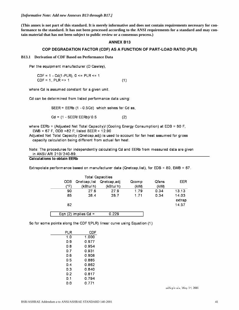
[Informative Note: Add new Annexes B13 through B17.]
(This annex is not part of this standard. It is merely informative and does not contain requirements necessary for con-formance to the standard. It has not been processed according to the ANSI requirements for a standard and may con-tain material that has not been subject to public review or a consensus process.)
ANNEX B13
COP DEGRADATION FACTOR (CDF) AS A FUNCTION OF PART-LOAD RATIO (PLR)
B13.1 Derivation of CDF Based on Performance Data
BSR/ASHRAE Addendum a to ANSI/ASHRAE STANDARD 140-2001 41

For real equipment, the representation of Figure 10 isreasonable for PLR greater than or equal to approximately 0.1;for PLR less than or equal to approximately 0.1, Figure 10indicates less efficiency degradation than that suggested bymore detailed information.A-7 However, real equipment thatcycles ON/OFF has controls that prevent operation at PLR lessthan or equal to approximately 0.05. For the purpose of testingsimulation software in the context of these analytical verifica-tion tests, Figure 10 is reasonable.
B13.2 PLR Definition Similarity
We have defined PLR in cases E100-E200 based on guid-
ance from the equipment manufacturer as
PLR1 = Qnet / CAPnet
where
Qnet = net refrigeration effect,
CAPnet = adjusted net total capacity.
We wish to check the equivalence of defining PLR as
PLR2 = Qgtc / CAPgtc
where
Qgtc = gross total coil load,
CAPgtc = gross total capacity.
The net refrigeration effect = Qgtc – Qfanwhere Qfan is the air distribution fan heat.
The adjusted net capacity = CAPgtc – Pfanwhere Pfan = fan rated power.
Then, for PLR1 = PLR2 to be true implies
Qgtc / CAPgtc = (Qgtc – Qfan) / (CAPgtc – Pfan),
which is true if
Qfan / Pfan = Qgtc / CAPgtc,
that is, if the fan heat for a given period is the fan’s run-timefraction for that period multiplied by the fan power, whereQgtc/CAPgtc inherently defines the required fraction of atime period that the evaporator coil is to be removing heat ata given capacity. The above relation is true if there is no addi-tional fan run time (and fan heat) associated with additionalcompressor start-up run time, which occurs during part-loadoperation.
For cases E100-E200, because the indoor fan cycles on/off with the compressor, we originally defined the net refrig-eration effect to subtract out fan heat for the time when thecompressor is operating (which is longer than the time that thecoil is actually removing heat at rated capacity).
For that situation, it is useful to think of
Qfan / Pfan = PLR / CDF.
However, this relation implies
Qfan / Pfan ≠ Qgtc / CAPgtc
with the theoretical result that PLR1 ≠ PLR2. An analysis of the difference between PLR1 and PLR2
and corresponding resultant CDF1 and CDF2 that could be
used in evaluating part-load performance is shown below inthe spreadsheet table. This analysis applies values of coilcapacity and fan power for the equipment at ARI rating condi-tions. From this analysis we observe (see far right column ofthe spreadsheet table) that the resulting difference betweenCDF1 and CDF2 and, therefore, the compressor energyconsumptions related to applying those CDFs, is <0.05%,which is negligible. Thus, we conclude that for the purpose ofcalculating CDF, either PLR1 or PLR2 may be used.
Note regarding the above spreadsheet table: The total fan
run-time fraction, including the additional start-up run time
during which no or little cooling occurs, = PLR/CDF. Actually,
fan heat should be slightly higher because the additional fan run
time due to CDF creates a slight amount of additional fan heat
that, in turn, causes slightly more additional run time. In accord
with the analytical solution by Dresden University of Technol-
ogy (discussed in informative Annex B17), the additional run
time (fan heat) for mid-PLR Case E170 is 0.5% greater if this
effect is taken into account. Since this is a 0.5% effect on a quan-
tity that makes up at most 4% of the total coil load (i.e., 0.02%
effect overall), then for the purpose of calculating CDF =
f(PLR) we ignore it.
(This annex is not part of this standard. It is merelyinformative and does not contain requirements necessaryfor conformance to the standard. It has not been pro-cessed according to the ANSI requirements for a stan-dard and may contain material that has not been subjectto public review or a consensus process.)
ANNEX B14
COOLING COIL BYPASS FACTOR
B14.1 IntroductionCalculation techniques provided here are for illustrative
purposes. Some models may have slight variations in thecalculation, including the use of enthalpy ratios rather thandry-bulb temperature ratios in Equation B14-1 (below), ordifferent specific heat assumptions for leaving air conditionsin Equation B14-3 (below), among others.
Cooling coil BF can be thought of as the fraction of thedistribution air that does not come into contact with the cool-ing coil; the remaining air is assumed to exit the coil at theaverage coil surface temperature (ADP). BF at ARI ratingconditions is approximately
0.049 ≤ BF ≤ 0.080.
42 BSR/ASHRAE Addendum a to ANSI/ASHRAE STANDARD 140-2001

The uncertainty surrounding this value is illustrated in thetwo examples for calculating BF from given manufacturerdata that are included in the rest of this annex, as well as fromseparate calculation results by Technische Universität Dres-den (TUD). The uncertainty can be traced to the calculatedADP (56.2°F) being different from the ADP listed by themanufacturer (56.8°F). Because we have been unable toacquire the manufacturer’s specific method for determiningADP, we have not been able to determine which ADP numberis better. However, the manufacturer has indicated that perfor-mance data are only good to within 5% of real equipmentperformance. So we can hypothesize that the listed versuscalculated ADP disagreements could be a consequence of thedevelopment of separate correlation equations for each perfor-mance parameter within the range of experimental uncer-tainty. Based on simulation sensitivity tests with DOE-2.1E,the above range of BF inputs causes total electricity consump-tion to vary by ±1%.
Calculations based on the listed performance data indi-cate that BF varies as a function of EDB, EWB, and ODB.Incorporate this aspect of equipment performance into yourmodel if your software allows it, using a consistent method fordeveloping all points of the BF variation map. (Note that sensi-tivity tests for cases E100–E200 using DOE-2.1E indicate thatassuming a constant value of BF—versus allowing BF to varyas a function of EWB and ODB—adds an additional ±1%uncertainty to the total energy consumption results for CaseE185 and less for the other cases.)
The equipment manufacturer recommends modeling theBF as independent of (not varying with) the PLR. This isbecause the airflow rate over the cooling coil is assumedconstant when the compressor is operating (fan cycles on/offwith compressor).
B14.2 Calculation of Coil Bypass Factor
B14.2.1 Nomenclature
ADP apparatus dew point (°F)
BF bypass factor (dimensionless)
cpa specific heat of dry air (Btu/lb°F)
cpw specific heat of water vapor (Btu/lb°F)
h1 enthalpy of air entering cooling coil (Btu/lb dry air)
h2 enthalpy of air leaving cooling coil (Btu/lb dry air)
qs gross sensible capacity (Btu/h)
qT gross total capacity (Btu/h)
Q indoor fan airflow rate (ft3/min)
Tdb1 entering dry-bulb temperature (°F)
Tdb2 leaving dry-bulb temperature (°F)
Twb1 entering wet-bulb temperature (°F)
w humidity ratio (lb water vapor/lb dry air)
ρr density of standard dry air at fan rating conditions (0.075 lb/ft3)
B14.2.2 Known InformationAir-Conditioning and Refrigeration Institute (ARI) Condi-tions:
• Tdb1 = 80°F• Twb1 = 67°F.
From Table 26d at ARI conditions:
• Q = 900 ft3/min• qs = 21700 Btu/h (gross sensible capacity)• qT = 27900 Btu/h (gross total capacity)• ADP = 56.8°F.
B14.2.3 Governing Equations
BF = (Tdb2 - ADP)/(Tdb1 - ADP) (Eq. B14-1)A-8
The following equations and related properties arecommonly used approximations for working with volumetricflow rates.A-9
qT = ρr Q (60 min/h) (h1 - h2) (Eq. B14-2)
qs = ρr Q (60 min/h) (cpa + cpw(w)) (Tdb1 - Tdb2) (Eq. B14-3)
ρr = 0.075 lb/ft3
cpa = 0.24 Btu/lb°F
cpw = 0.45 Btu/lb°F
w ≈ 0.01 lb water vapor/lb dry air.
So for these English units, Equations (B14-2) and (B14-3) become:
qT = 4.5 Q (h1 - h2) (Eq. B14-2a)
qs = 1.10 Q (Tdb1 - Tdb2) (Eq. B14-3a)
B14.2.4 Solution Technique Using ADP Calculated byExtending the Condition Line to the Saturation Curve.
To find ADP, extend the condition line of the systemthrough the saturation curve on the psychrometric chart.A-10
The condition line is the line going through coil enteringconditions with slope determined by sensible heat ratio for thegiven operating conditions.A-8 This example is illustrated onthe psychrometric chart in Figure B14-2. To draw the condi-tion line, State 2 must be determined; State 1 is ARI conditions(Tdb1 = 80.0°F, Twb1 = 67°F). Defining State 2 requires twoindependent properties that can be identified from Equations(B14-2) and (B14-3).
Solve for h2 using Equation (B14-2) with qT = 27,900Btu/h and Q = 900 ft3/min. From ideal gas equationscommonly used for psychrometrics,1 at ARI conditions h1 =31.45 Btu/lb dry air. These values applied to Equation (B14-2) give:
Figure B14-1 System schematic.
BSR/ASHRAE Addendum a to ANSI/ASHRAE STANDARD 140-2001 43

44 BSR/ASHRAE Addendum a to ANSI/ASHRAE STANDARD 140-2001
Fig
ure
B14
-2A
DP
cal
cula
tion
.

h2 = 24.55 Btu/lb dry air.
Solving for Tdb2 using Equation (B14-3) with Tdb1 =80°F, qs = 21700 Btu/h, and Q = 900 ft3/min gives:
Tdb2 = 58.1°F.
On the psychrometric chart, drawing a line through thesetwo states and extending it to the saturation curve gives:
ADP = 56.2°F.
Solving Equation (B14-1) using Tdb1 = 80°F, Tdb2 =58.1°F, and ADP = 56.2°F gives:
BF = 0.080
B14.2.5 Solution Technique Using ADP Listed in Per-formance Data
Solving Equation (B14-1) using Tdb1 = 80°F, Tdb2 =58.1°F, and ADP = 56.8°F gives:
BF = 0.055
B14.2.6 Solution by TUD
The TRNSYS-TUD modeler report in Part III of HVACBESTESTA-5 indicates that:
BF = 0.049
This solution is based on manufacturer-listed values ofADP.
B14.3 Conclusions
The BF for this system at ARI conditions is approxi-mately in the range of:
0.049 ≤ BF ≤ 0.080
Some uncertainty is associated with the governing equa-tions and related properties commonly used for calculatingleaving air conditions; these equations are approximations. Inaddition, some uncertainty is associated with using thepsychrometric chart to find the ADP (56.2°F) in the first solu-tion. Finally, there may be additional uncertainty related to themethodology for developing ADP. For example, the results ofEquation B14-1 can be slightly different if enthalpy ratios areused in place of dry bulb temperature ratios. Also, documen-tation of how the manufacturer calculated its listed ADP wasunavailable, and the source code for manufacturer softwareused to develop catalog data is proprietary.
Based on sensitivity tests with DOE-2.1E:
• The above range of BF inputs causes total electricityconsumption to vary by ±1%.
• Assuming a constant value of BF versus allowing BF tovary as a function of EWB and ODB adds an additional±1% uncertainty to the total energy consumption resultsfor Case E185, and less for the other cases.
(This annex is not part of this standard. It is merelyinformative and does not contain requirements necessaryfor conformance to the standard. It has not been pro-cessed according to the ANSI requirements for a stan-dard and may contain material that has not been subjectto public review or a consensus process.)
ANNEX B15
INDOOR FAN DATA EQUIVALENCEFan performance data for indoor fan power (230 W) and
airflow rate (900 CFM = 0.425 m3/s) are based on dry air atstandard fan rating conditions. ASHRAE defines a standardcondition as 1 atmosphere (101.325 kPa or 14.696 psi) and68°F (20°C) with a density of 0.075 lb/ft3 (1.204 kg/m3).A-9
The fan efficiency of 0.5 is based on a discussion with theunitary system manufacturer.
The total fan pressure is based on:A-11
Eff = Q * ∆P / W
where
Q ≡ indoor fan airflow rate (m3/s)
∆P ≡ total fan pressure (Pa)
W ≡ fan electric power input (W)
Eff ≡ total fan plus motor and drive efficiency (motor/drive in air stream).
Solving for ∆P,
∆P = W * Eff / Q
= 230 W * 0.5 / 0.425 m3/s = 271 Pa = ∆P.
The supply air temperature rise from fan heat is based on
qfan = ρ* cp * Q * ∆T * C
where
qfan ≡ fan heat (Btu/h or W),
ρ ≡ standard air density = 0.075 lb/ft3 (1.204 kg/m3),
cp ≡ specific heat of air (Btu/(lb°F) or kJ/(kgK)),
Q ≡ indoor fan airflow rate (ft3/min or m3/s),
∆T ≡ supply air temperature rise from fan heat (°F or °C),
C ≡ units conversion constant.
Solving for ∆T,
∆T = qfan / (ρ* cp * Q *C)
where
qfan = 230 W = 785 Btu/h; Q = 900 CFM = 0.425 m3/s,
cp = 0.24 Btu/lb F for dry air, or
cp = 0.2445 Btu/lb F when humidity ratio = 0.01.A-9
Then, ∆T = 785 Btu/h / {0.075 lb/ft3 * 900 ft3/min * 60min/h * 0.2445 Btu/(lb°F)}
∆T = 0.793°F (0.441 °C)
or
for cp = 0.24 Btu/(lb°F), ∆T = 0.808°F (0.449°C).
BSR/ASHRAE Addendum a to ANSI/ASHRAE STANDARD 140-2001 45

(This annex is not part of this standard. It is merelyinformative and does not contain requirements necessaryfor conformance to the standard. It has not been pro-cessed according to the ANSI requirements for a stan-dard and may contain material that has not been subjectto public review or a consensus process.)
ANNEX B16
QUASI-ANALYTICAL SOLUTION RESULTS AND EXAMPLE SIMULATION RESULTS FOR HVAC
EQUIPMENT PERFORMANCE TESTS
B16.1 IntroductionThe results from quasi-analytical solutions and various
detailed building energy simulation programs applied to thetests of Section 5.3 are presented here in tabular and graphicform. These results can be used for a comparison with the soft-ware being tested. Alternatively, a user can run a number ofdifferent programs through the Standard Method of Test orgenerate their own quasi-analytical solution results and drawcomparisons from those results independently or in conjunc-tion with the results listed here. In either case, when makingcomparisons the user should employ the diagnostic logicpresented in informative Annex B9.
For convenience to users who wish to plot or tabulate theirresults along with the example results, an electronic version of thequasi-analytical solution results and example simulation resultshas been included with the spreadsheet file RESULTS5-3.XLS inthe accompanying files (available at http://www.ashrae.org/template/PDFDetail?assetID=34505). Spreadsheet navigationinstructions are included in RESULTS5-3.DOC and have beenprinted out in informative Annex B10, Section B10.2 for conve-nience.
B16.2 Importance of Quasi-Analytical Solution ResultsA characteristic difference between the Annex B8 results
for the building thermal envelope and fabric load tests versusthe Annex B16 results for the HVAC equipment performancetests is that the Annex B16 results include quasi-analyticalsolutions. In general, it is difficult to develop worthwhile testcases that can be solved analytically or quasi-analytically, butsuch solutions are extremely useful when possible. Analyticalor quasi-analytical solutions represent a “mathematical truthstandard”; that is, given the underlying physical assumptionsin the case definitions, there is a mathematically correct solu-tion for each case. In this context, the underlying physicalassumptions regarding the mechanical equipment as definedin cases E100-E200 are representative of typical manufacturerdata normally used by building design practitioners. Many“whole-building” simulation programs are designed to workwith this type of data.
It is important to understand the difference between a“mathematical truth standard” and an “absolute truth stan-dard.” In the former, we accept the given underlying physicalassumptions while recognizing that these assumptions repre-sent a simplification of physical reality. The ultimate or “abso-lute” validation standard would be comparison of simulationresults with a perfectly performed empirical experiment, theinputs for which are perfectly specified to the simulationists.In reality, an experiment is performed and the experimentalobject is specified within some acceptable range of uncer-tainty. Such experiments are possible, but expensive. Werecommend developing a set of empirical validation experi-ments in the future.
The minor disagreements among the two sets of quasi-analytical solution results presented in Annex B16 are smallenough to allow identification of bugs in the software thatwould not otherwise be apparent from comparing softwareonly to other software and therefore improves the diagnosticcapabilities of the test procedure. Further discussion of howquasi-analytical solutions were developed is included inAnnex B17.
B16.3 Example Simulation ResultsBecause the quasi-analytical solution results constitute a
reliable set of theoretical results (a mathematical truth stan-dard), the primary purpose of including simulation results forthe E100–E200 cases in Annex B16 is to allow simulationists tocompare their relative agreement (or disagreement) versus thequasi-analytical solution results to that for other simulationresults. Perfect agreement among simulations and quasi-analyt-ical solutions is not necessarily expected. The results give anindication of what sort of agreement is possible between simu-lation results and the quasi-analytical solution results.
Because the physical assumptions of a simulation may bedifferent from those for the quasi-analytical solutions, a testedprogram may disagree with the quasi-analytical solutionswithout necessarily being incorrect. However, it is worthwhileto investigate the source of differences, as the collective expe-rience of the authors of this standard is that such differencesoften indicate problems with the software or its usage, includ-ing, but not limited to, (a) user input error, where the user misinterpreted or
mis-entered one or more program inputs;(b) problem with a particular algorithm in the program;(c) one or more program algorithms used outside their
intended range.For generating simulation results, along with using
consistent modeling methods, simulationists were requestedto use the most detailed modeling methods their softwareallows. The example simulation results were the product ofnumerous iterations to incorporate clarifications to the test spec-ification, simulation input deck corrections, and simulationsoftware improvements. For a summary of how quasi-analyt-ical solution and simulation results were developed see infor-mative Annex B17. For more detailed information about theseresults see HVAC BESTEST.A-5
B16.4 NomenclatureResults are grouped by case numbers, e.g., “E100” is Case
E100 (Section 5.3.1). Sensitivity results are listed using twocase numbers separated by a minus sign, e.g., “E110-100” isthe difference between Case E110 (Section 5.3.2.1.1) andCase E100.
Analytical quasi-analytical solution
ARI Air-Conditioning & Refrigeration Institute
CA-SIS CA-SIS VI (see Table B17-1)
CIEMAT Centro de Investigaciones Energeticas, Medioambientales y Technologicas
CLM2000 CLIM2000 2.1.6 (see Table B17-1)
COP coefficient of performance
Delta sensitivity between listed cases
46 BSR/ASHRAE Addendum a to ANSI/ASHRAE STANDARD 140-2001
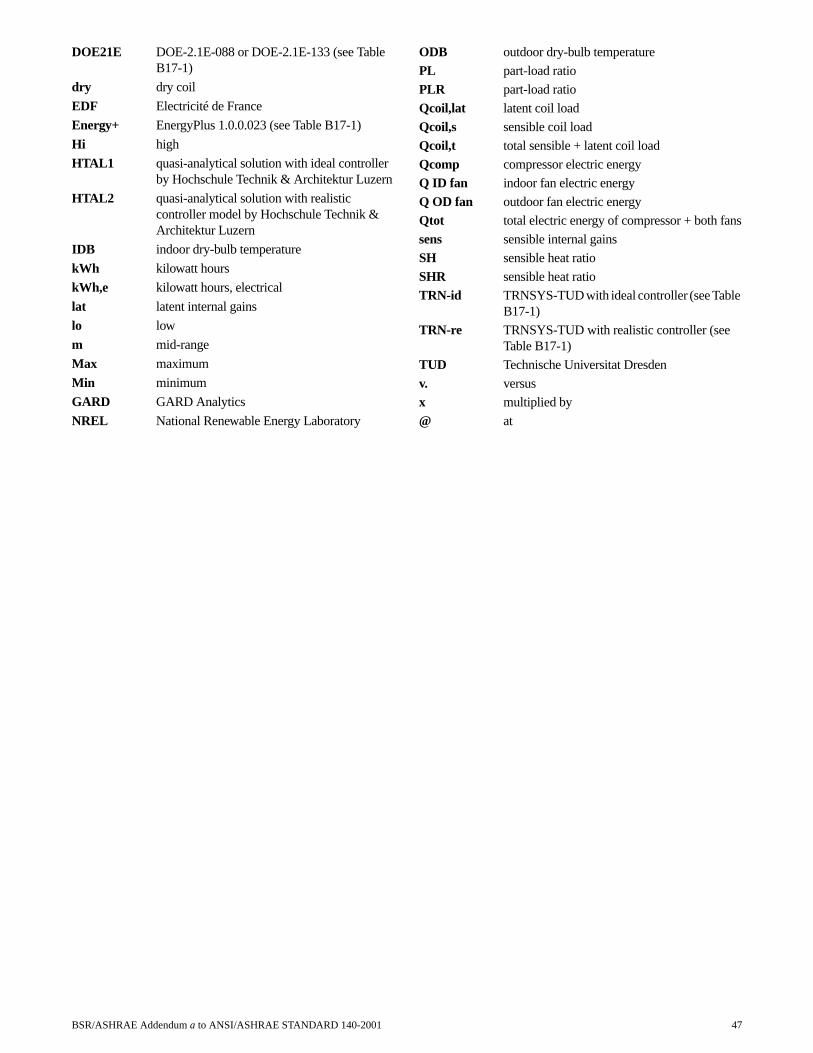
DOE21E DOE-2.1E-088 or DOE-2.1E-133 (see Table B17-1)
dry dry coil
EDF Electricité de France
Energy+ EnergyPlus 1.0.0.023 (see Table B17-1)
Hi high
HTAL1 quasi-analytical solution with ideal controller by Hochschule Technik & Architektur Luzern
HTAL2 quasi-analytical solution with realistic controller model by Hochschule Technik & Architektur Luzern
IDB indoor dry-bulb temperature
kWh kilowatt hours
kWh,e kilowatt hours, electrical
lat latent internal gains
lo low
m mid-range
Max maximum
Min minimum
GARD GARD Analytics
NREL National Renewable Energy Laboratory
ODB outdoor dry-bulb temperature
PL part-load ratioPLR part-load ratio
Qcoil,lat latent coil loadQcoil,s sensible coil load
Qcoil,t total sensible + latent coil load
Qcomp compressor electric energyQ ID fan indoor fan electric energy
Q OD fan outdoor fan electric energyQtot total electric energy of compressor + both fans
sens sensible internal gainsSH sensible heat ratio
SHR sensible heat ratioTRN-id TRNSYS-TUD with ideal controller (see Table
B17-1)TRN-re TRNSYS-TUD with realistic controller (see
Table B17-1)TUD Technische Universitat Dresden
v. versusx multiplied by
@ at
BSR/ASHRAE Addendum a to ANSI/ASHRAE STANDARD 140-2001 47

48 BSR/ASHRAE Addendum a to ANSI/ASHRAE STANDARD 140-2001

BSR/ASHRAE Addendum a to ANSI/ASHRAE STANDARD 140-2001 49

50 BSR/ASHRAE Addendum a to ANSI/ASHRAE STANDARD 140-2001

BSR/ASHRAE Addendum a to ANSI/ASHRAE STANDARD 140-2001 51

52 BSR/ASHRAE Addendum a to ANSI/ASHRAE STANDARD 140-2001
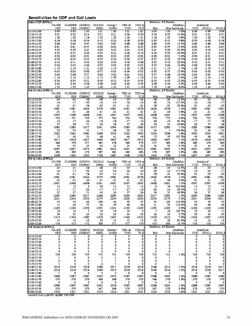
BSR/ASHRAE Addendum a to ANSI/ASHRAE STANDARD 140-2001 53

54 BSR/ASHRAE Addendum a to ANSI/ASHRAE STANDARD 140-2001

BSR/ASHRAE Addendum a to ANSI/ASHRAE STANDARD 140-2001 55

56 BSR/ASHRAE Addendum a to ANSI/ASHRAE STANDARD 140-2001

BSR/ASHRAE Addendum a to ANSI/ASHRAE STANDARD 140-2001 57

58 BSR/ASHRAE Addendum a to ANSI/ASHRAE STANDARD 140-2001

BSR/ASHRAE Addendum a to ANSI/ASHRAE STANDARD 140-2001 59

60 BSR/ASHRAE Addendum a to ANSI/ASHRAE STANDARD 140-2001

BSR/ASHRAE Addendum a to ANSI/ASHRAE STANDARD 140-2001 61

62 BSR/ASHRAE Addendum a to ANSI/ASHRAE STANDARD 140-2001

BSR/ASHRAE Addendum a to ANSI/ASHRAE STANDARD 140-2001 63

64 BSR/ASHRAE Addendum a to ANSI/ASHRAE STANDARD 140-2001

BSR/ASHRAE Addendum a to ANSI/ASHRAE STANDARD 140-2001 65

66 BSR/ASHRAE Addendum a to ANSI/ASHRAE STANDARD 140-2001
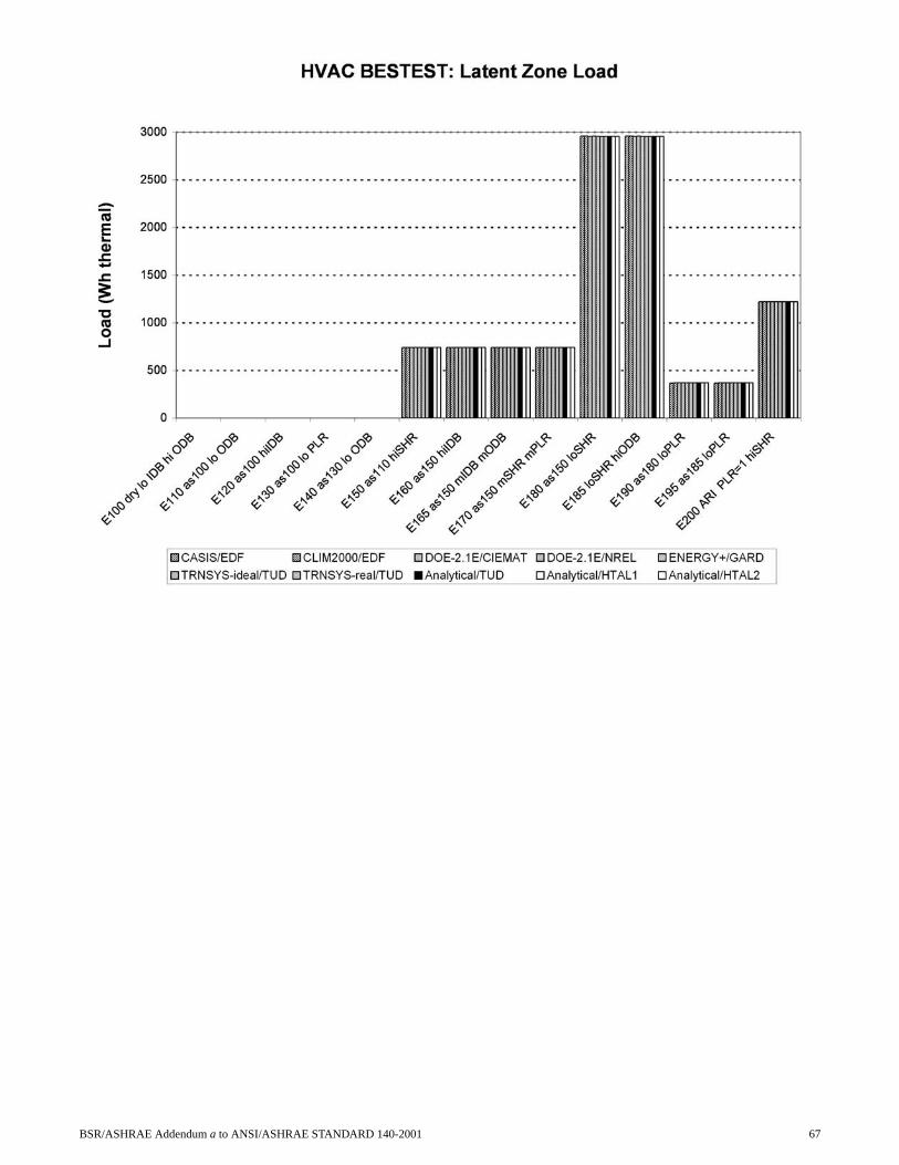
BSR/ASHRAE Addendum a to ANSI/ASHRAE STANDARD 140-2001 67

68 BSR/ASHRAE Addendum a to ANSI/ASHRAE STANDARD 140-2001

(This annex is not part of this standard. It is merelyinformative and does not contain requirements necessaryfor conformance to the standard. It has not been pro-cessed according to the ANSI requirements for a stan-dard and may contain material that has not been subjectto public review or a consensus process.)
ANNEX B17
PRODUCTION OF QUASI-ANALYTICAL SOLUTION RESULTS AND EXAMPLE SIMULATION RESULTS
B17.1 IntroductionThe full discussion regarding production of quasi-analyt-
ical solution results and example simulation results is includedin HVAC BESTEST.A-5 Portions of that discussion have beenincluded here. The quasi-analytical solutions and programsused to generate the example simulation results are describedin Table B17-1.
The first column of Table B17-1 (“Model”) indicates theproper program name and version number or indicates a quasi-
analytical solution. The second column (“Authoring Organi-zation”) indicates the national research facility or universitywith expertise in building science that wrote the simulationsoftware or did the quasi-analytical solutions. The thirdcolumn (“Implemented By”) indicates the national researchfacility or university with expertise in building science thatperformed the simulations or did the quasi-analytical solu-tions. The entries in the fourth column are the abbreviationsfor the simulations and quasi-analytical solutions generallyused in Annex B16 and elsewhere in the informative annexes.The majority of participating organizations that performedsimulations ran software that their organization eitherauthored or coauthored.
The availability of quasi-analytical solutions (see SectionB17.2) greatly helped to identify and correct errors in thesimulations such that errors are minimized in the final simu-lation results. Also, to minimize the potential for user error inthe simulations, when feasible, more than one modeler devel-oped input files for each program. This was done for DOE-2.1E and where disagreement in the inputs or results was
TABLE B17-1
Participating Organizations and Computer Programs
Model Authoring Organization Implemented By Abbreviation
Quasi-analytical solution with ideal controller model
Hochschule Technik & Architektur Luzern, Switzerland (HTAL)
Hochschule Technik & Architektur Luzern, Switzerland
HTAL1
Quasi-analytical solution with realistic controller model
Hochschule Technik & Architektur Luzern, Switzerland
Hochschule Technik & Architektur Luzern, Switzerland
HTAL2
Quasi-analytical solution with ideal controller model
Technische Universität Dresden, Germany (TUD)
Technische Universität Dresden, Germany
TUD
CA-SIS V1 Electricité de France, France (EDF) Electricité de France, France CA-SIS
CLIM2000 2.1.6 Electricité de France, France Electricité de France, France CLM2000
DOE-2.1E-088 LANL/LBNL/ESTSC,a,b,c USA CIEMAT,d Spain DOE21E/CIEMAT
DOE-2.1E-133 LANL/LBNL/JJH,a,b,e USA NREL/JNA,f USA DOE21E/NREL
ENERGYPLUS 1.0.0.023 LBNL/UIUC/CERL/OSU/GARD Analytics/FSEC/DOE-OBT,a,g,h,i,j,k
GARD Analytics, USA Energy+
TRNSYS 14.2-TUD with ideal controller model
University of Wisconsin, USA; Technische Universität Dresden, Ger.
Technische Universität Dresden, Germany
TRN-idTRNSYS-ideal
TRNSYS 14.2-TUD with real controller model
University of Wisconsin, USA; Technische Universität Dresden, Ger.
Technische Universität Dresden, Germany
TRN-reTRNSYS-real
aLANL: Los Alamos National LaboratorybLBNL: Lawrence Berkeley National LaboratorycESTSC: Energy Science and Technology Software Center (at Oak Ridge National Laboratory, USA)dCIEMAT: Centro de Investigaciones Energeticas, Medioambientales y TecnologicaseJJH: James J. Hirsch & AssociatesfNREL/JNA: National Renewable Energy Laboratory/J. Neymark & AssociatesgUIUC: University of Illinois Urbana/ChampaignhCERL: U.S. Army Corps of Engineers, Construction Engineering Research LaboratoriesiOSU: Oklahoma State UniversityjFSEC: University of Central Florida, Florida Solar Energy CenterkDOE-OBT: U.S. Department of Energy, Office of Building Technology, State and Community Programs, Energy Efficiency and Renewable
Energy
BSR/ASHRAE Addendum a to ANSI/ASHRAE STANDARD 140-2001 69

found, the modelers worked to resolve the differences. Addi-tionally, one of the participants (TUD) developed quasi-analytical solutions and ran separate controller models withinTRNSYS; this allowed for greater understanding of the testspecification and of their simulation model. Where only asingle modeler was involved, we strongly recommended thatanother modeler familiar with the program check the inputscarefully.
Input decks used to generate the simulation results are providedin the files accompanying this standard (available at http://www.ashrae.org/template/PDFDetail?assetID=34505); see theREADME.DOC file. International Energy Agency participants thatran simulations for CA-SIS and CLIM2000 did not supply inputdecks with their results.
B17.2 Quasi-Analytical Solution ResultsThe quasi-analytical solution results given in Annex B16
were developed as part of International Energy Agency (IEA)Solar Heating and Cooling Programme Task 22. The impor-tance of having analytical or quasi-analytical solution resultsis discussed in Annex B16 (Section B16.2). Two of the IEAparticipating organizations independently developed quasi-analytical solutions that were submitted to a third party forreview.A-12, A-13, A-14 Comparing the results indicated somedisagreements, which were then resolved by allowing thesolvers to review the third-party reviewers’ comments and toreview and critique each others’ solution techniques. Thisprocess resulted in both solvers making logical and non-arbi-trary changes to their solutions such that their final results aremostly well within a <1% range of disagreement. Remainingdifferences in the quasi-analytical solutions are due in part tothe difficulty of completely describing boundary conditions.In this case the boundary conditions are a compromisebetween full reality and some simplification of the real phys-ical system that is mathematically solvable. Therefore, thequasi-analytical solutions have some element of interpretationof the exact nature of the boundary conditions that causesminor differences in the results. For example, in the modelingof the controller, one group derived a quasi-analytical solutionfor an “ideal” controller (that maintains zone temperatureexactly at the thermostat setpoint) while another group devel-oped a numerical solution for a “realistic” controller (thatallows a small degree of zone temperature variation over veryshort simulation time steps). As another example, for thepurpose of determining the “maximum EWB” dry-coil condi-tion, one group used linear interpolation or extrapolation inconjunction with local intervals of given performance data,while another group used a similar but more generalized solu-tion technique and incorporated the extremes of performancedata. Each quasi-analytical solution yields slightly differentresults, but all are correct in the context of this exercise. Thismay be less than perfect from a mathematician’s viewpoint butquite acceptable from an engineering perspective. A fullydetailed presentation of the quasi-analytical solutions, includ-ing specific examples of remaining minor differences in thesolutions, are discussed in Part II of HVAC BESTEST.A-5
B17.3 Selection of Programs for Producing ExampleSimulation Results
The criteria for selection of programs used for producingexample results required that
(a) the program be a true simulation based on hourly weatherdata and calculational time increments of one hour or lessand
(b) the program be representative of the state of the art inwhole-building energy simulation as defined by the IEAcountry making the selection.The programs used to generate example results have been
subjected to extensive prior validation testing. Such testingincludes the preliminary trials of HVAC BESTEST A-5 that ranfrom 1997 through 2001. The programs (to various extents)were also subjected to other comparative, empirical validationand/or analytical verification tests such as those referenced inHVAC BESTEST, IEA BESTEST, and in International BuildingPerformance Simulation Association (IBPSA) proceed-ings.14,21,22, A-5
(This annex is not part of this standard. It is merelyinformative and does not contain requirements necessaryfor conformance to the standard. It has not been pro-cessed according to the ANSI requirements for a stan-dard and may contain material that has not been subjectto public review or a consensus process.)
ANNEX B18
VALIDATION METHODOLOGIES AND OTHER RESEARCH RELEVANT TO STANDARD 140
[Informative Note: Delete Annex B13 and replace with newAnnex B18 as follows.]
B18.1 Overall Validation MethodologyAn overall validation methodology consists of three parts:
(a) Comparative Testing - in which a program is compared toitself or to other programs
(b) Analytical Verification - in which the output from a pro-gram, subroutine, algorithm, or software object is com-pared to the result from a known analytical or quasi-analytical solution for isolated heat transfer mechanismsunder very simple and highly constrained boundary con-ditions
(c) Empirical Validation - in which calculated results from aprogram, subroutine, algorithm, or software object arecompared to monitored data from a real building, test cell,or laboratory experiment Table B18-1 shows the advantages and disadvantages of
these three techniques.A-15, A-5 Defining two terms is useful ininterpreting Table 1. Here a “model” is the representation ofreality for a given physical behavior. For example, one way tomodel heat transfer through a wall is by using a simplifyingassumption of one-dimensional conduction. An alternative(more detailed) model for wall heat transfer could employ two-dimensional conduction. The “solution process” is a term thatencompasses the mathematics and computer coding to solve agiven model (e.g., a finite difference approximation to solve adifferential equation) and the technique for integrating individ-ual models and boundary conditions into an overall solutionmethodology—such as an iterative energy balance throughlayers of a single wall, over all the surfaces of a given zone, orbetween a zone(s) and its related mechanical system(s). Thesolution process for a model can be perfect, while the model
70 BSR/ASHRAE Addendum a to ANSI/ASHRAE STANDARD 140-2001
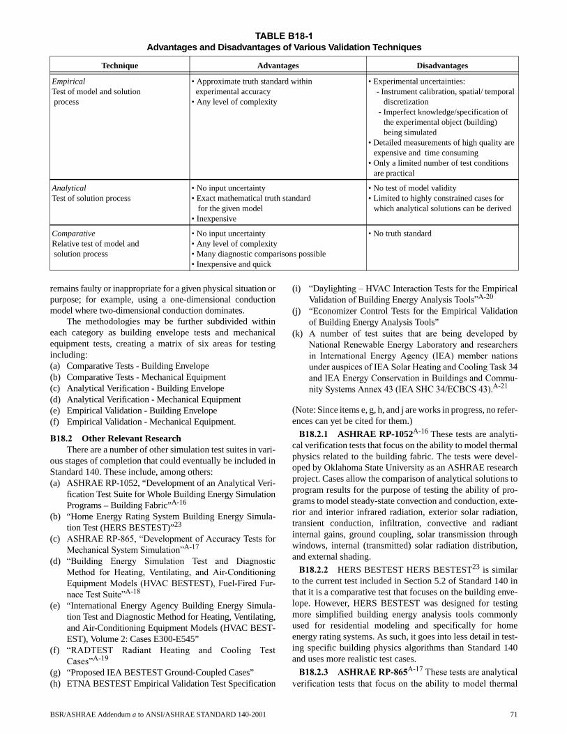
remains faulty or inappropriate for a given physical situation orpurpose; for example, using a one-dimensional conductionmodel where two-dimensional conduction dominates.
The methodologies may be further subdivided withineach category as building envelope tests and mechanicalequipment tests, creating a matrix of six areas for testingincluding:(a) Comparative Tests - Building Envelope(b) Comparative Tests - Mechanical Equipment(c) Analytical Verification - Building Envelope(d) Analytical Verification - Mechanical Equipment(e) Empirical Validation - Building Envelope (f) Empirical Validation - Mechanical Equipment.
B18.2 Other Relevant Research There are a number of other simulation test suites in vari-
ous stages of completion that could eventually be included inStandard 140. These include, among others:(a) ASHRAE RP-1052, “Development of an Analytical Veri-
fication Test Suite for Whole Building Energy SimulationPrograms – Building Fabric”A-16
(b) “Home Energy Rating System Building Energy Simula-tion Test (HERS BESTEST)”23
(c) ASHRAE RP-865, “Development of Accuracy Tests for
Mechanical System Simulation”A-17
(d) “Building Energy Simulation Test and Diagnostic
Method for Heating, Ventilating, and Air-Conditioning
Equipment Models (HVAC BESTEST), Fuel-Fired Fur-
nace Test Suite”A-18
(e) “International Energy Agency Building Energy Simula-tion Test and Diagnostic Method for Heating, Ventilating,and Air-Conditioning Equipment Models (HVAC BEST-EST), Volume 2: Cases E300-E545”
(f) “RADTEST Radiant Heating and Cooling Test
Cases”A-19
(g) “Proposed IEA BESTEST Ground-Coupled Cases”(h) ETNA BESTEST Empirical Validation Test Specification
(i) “Daylighting – HVAC Interaction Tests for the Empirical
Validation of Building Energy Analysis Tools”A-20
(j) “Economizer Control Tests for the Empirical Validationof Building Energy Analysis Tools”
(k) A number of test suites that are being developed by
National Renewable Energy Laboratory and researchers
in International Energy Agency (IEA) member nations
under auspices of IEA Solar Heating and Cooling Task 34
and IEA Energy Conservation in Buildings and Commu-
nity Systems Annex 43 (IEA SHC 34/ECBCS 43).A-21
(Note: Since items e, g, h, and j are works in progress, no refer-ences can yet be cited for them.)
B18.2.1 ASHRAE RP-1052A-16 These tests are analyti-cal verification tests that focus on the ability to model thermalphysics related to the building fabric. The tests were devel-oped by Oklahoma State University as an ASHRAE researchproject. Cases allow the comparison of analytical solutions toprogram results for the purpose of testing the ability of pro-grams to model steady-state convection and conduction, exte-rior and interior infrared radiation, exterior solar radiation,transient conduction, infiltration, convective and radiantinternal gains, ground coupling, solar transmission throughwindows, internal (transmitted) solar radiation distribution,and external shading.
B18.2.2 HERS BESTEST HERS BESTEST23 is similarto the current test included in Section 5.2 of Standard 140 inthat it is a comparative test that focuses on the building enve-lope. However, HERS BESTEST was designed for testingmore simplified building energy analysis tools commonlyused for residential modeling and specifically for homeenergy rating systems. As such, it goes into less detail in test-ing specific building physics algorithms than Standard 140and uses more realistic test cases.
B18.2.3 ASHRAE RP-865A-17 These tests are analytical
verification tests that focus on the ability to model thermal
TABLE B18-1
Advantages and Disadvantages of Various Validation Techniques
Technique Advantages Disadvantages
EmpiricalTest of model and solution process
• Approximate truth standard within experimental accuracy
• Any level of complexity
• Experimental uncertainties: - Instrument calibration, spatial/ temporal
discretization - Imperfect knowledge/specification of
the experimental object (building) being simulated
• Detailed measurements of high quality are expensive and time consuming
• Only a limited number of test conditions are practical
AnalyticalTest of solution process
• No input uncertainty• Exact mathematical truth standard for the given model• Inexpensive
• No test of model validity• Limited to highly constrained cases for
which analytical solutions can be derived
ComparativeRelative test of model and solution process
• No input uncertainty• Any level of complexity• Many diagnostic comparisons possible• Inexpensive and quick
• No truth standard
BSR/ASHRAE Addendum a to ANSI/ASHRAE STANDARD 140-2001 71

physics related to the air-side of mechanical equipment. The
tests were developed by Pennsylvania State University and
Texas A&M University as an ASHRAE research project.
Cases allow the comparison of quasi-analytical solutions to
program results for the purpose of testing the ability of pro-
grams to model air-side mechanical equipment and systems.
These tests are subdivided by system type, for example, con-
stant-volume dual duct or variable-volume single duct with
reheat.
B18.2.4 HVAC BESTEST Fuel-Fired Furnace Test
SuiteA-18 is an analytical verification test that also has some
comparative test components, developed by the CANMET
Energy Technology Centre of Natural Resources Canada in
conjunction with the International Energy Agency (IEA)
Solar Heating and Cooling (SHC) Programme Task 22. This
test focuses on the ability to model residential fuel-fired fur-
nace mechanical equipment and could directly append the
unitary mechanical equipment cases of Section 5.3. Cases
allow the comparison of quasi-analytical solutions to program
results for the purpose of testing the ability of programs to
model steady-state efficiency, fuel consumption, variation of
furnace performance with part-load ratio, air-distribution fan
operation, and combustion-air fan operation.
B18.2.5 HVAC BESTEST Cases E300-E545 is a com-parative test being developed by the National RenewableEnergy Laboratory in conjunction with the InternationalEnergy Agency Solar Heating and Cooling Programme Task22. This test suite extends the unitary space cooling equip-ment tests of Section 5.3. The cases are more realistic (includ-ing more dynamic loading and weather conditions) andcannot be solved analytically or quasi-analytically. Casesinclude variation of PLR, ODB, and EDB for both dry-coiland wet-coil conditions. Also tested in the dynamic context isthe ability of programs to model equipment performance withoutside air mixing, infiltration loading, thermostat set-up,undersized equipment, and economizers with various temper-ature and enthalpy controls.
B18.2.6 RADTESTA-19 is a comparative test developed
by Hochschule fur Technik + Architektur Luzern in conjunc-
tion with the IEA SHC Task 22. Cases allow the comparison
of program results to each other for the purpose of testing the
ability of programs to model radiant heating or cooling
hydronic loop systems embedded in the building shell (e.g.,
floor, ceiling, etc.).
B18.2.7 Proposed IEA BESTEST Ground-CoupledCases is a comparative test being developed by the NationalRenewable Energy Laboratory in conjunction with the IEASolar Heating and Cooling Programme. These cases focus onthe ability to model ground-coupled heat transfer and coulddirectly append the building fabric cases of Section 5.2. Casesallow the comparison of program results to each other for thepurpose of testing the ability of programs to model interactionof the building with the atmosphere through the ground,effects of solar radiation on ground-coupled surfaces, effectsof calculated film coefficients versus constant film coeffi-cients, slab-on-grade geometries with and without insulation,
basement geometries with and without insulation, interactionof the building with the deep ground conditions including heatsinks such as water tables, and walkout basement construc-tion. Additional in-depth cases are being developed to deter-mine the causes for disagreements among detailed modelresults found in the preceding test cases. The new test casescompare ground models integrated with whole-building sim-ulations to independent detailed models. There is also an ana-lytical verification test case for checking the independentdetailed models and for checking that such models are prop-erly applied by users. Parametric variations versus a steady-state slab-on-grade base case include periodic ground surfacetemperature variation (versus steady-state), floor slab aspectratio, slab size, deep ground temperature depth, and interiorand exterior convective coefficients (realistic versus high val-ues to test the effect of surface temperature uniformity).
B18.2.8 ETNA BESTEST is an empirical validation testbeing developed by Electricité de France in conjunction withJ. Neymark & Associates and the National Renewable EnergyLaboratory. Cases allow the comparison of empirical data toprogram results, allowing for validation of models within theuncertainty of the experiments. Test cases focus on the abilityto model thermal loads associated with the building fabric inartificial and natural climatic configurations. Parametric vari-ations in a natural climate configuration include dynamicthermal diffusion (with windows insulated and covered), solargains (windows uncovered), thermostat setback, variation ofinterior surface convective coefficient (by varying mixing fanflow rate), variation of heater type, variation of thermal mass(insulation over the floor slab), and interactions of these. Para-metric variations in an artificial climate configuration includetests for the ability to model outside air ventilation/infiltra-tion, internal gains, and typical wall mounted “convective”and “radiant” heaters versus a heater designed for ideal pureconvective output with uniform mixing of zone air (com-monly assumed by simulations). Data were gathered in theartificial climate configuration to empirically characterizesteady-state overall building heat loss coefficient; steady-statethermal conductance of individual walls, floor, ceiling, andwindows; and internal thermal capacitance. Measurementswere also made with the objectives of estimating interior con-vective surface coefficients and empirically characterizingincidence-angle-dependent window optical transmittance.
B18.2.9 Daylighting – HVAC Interaction Tests for the
Empirical Validation of Building Energy Analysis ToolsA-
20 were developed by Iowa State University and Iowa Energy
Resource Station in conjunction with IEA SHC Task 22.
Cases allow the comparison of empirical data to program
results, allowing for validation of models within the uncer-
tainty of the experiments. The tests focus on the ability to
model daylighting/HVAC interaction. Identical rooms con-
nected to separate mechanical systems are used with the dif-
ference that one room has dimmable ballasts; interior
illuminance, solar irradiance, and heating loads were mea-
sured in both rooms.
B18.2.10 Economizer Control Tests for the EmpiricalValidation of Building Energy Analysis Tools are beingdeveloped by Iowa State University and Iowa Energy
72 BSR/ASHRAE Addendum a to ANSI/ASHRAE STANDARD 140-2001

Resource Station in conjunction with IEA SHC Task 22.Cases allow the comparison of empirical data to programresults, allowing for validation of models within the uncer-tainty of the experiments. The test cases focus on the abilityto model economizer control and outdoor air in VAV Systems.Parametric variations of economizer control tests include out-side air versus return air temperature comparison, with para-metric variations for 0% and 20% minimum outside air, andoutside air versus return air enthalpy comparison with 0%minimum outside air.
B18.3 Recommended Additional Research. The addi-tional tests listed in B18.2 do not cover the following areas:(a) Comparative Tests – Mechanical Equipment (Additional
tests beyond those in HVAC BESTEST unitary coolingand heating equipment cases)
(b) Analytical Verification – Mechanical Equipment (Addi-tional tests beyond those in RP-865 and HVAC BEST-EST unitary cooling and heating equipment cases)
(c) Empirical Validation - Mechanical Equipment (Addi-tional tests beyond those in IEA SHC Task 22 describedabove).More work to develop such Methods of Test is recom-
mended.
Informative Note: Renumber Section B14, References, asSection B19 and divide it into two parts, Section B19.1, whichcontains the references in the current standard, and SectionB19.2, which adds the new references for Addendum a.
(This annex is not part of this standard. It is merelyinformative and does not contain requirements necessaryfor conformance to the standard. It has not been pro-cessed according to the ANSI requirements for a stan-dard and may contain material that has not been subjectto public review or a consensus process.)
ANNEX B194
REFERENCES
B19.1 References for ANSI/ASHRAE Standard 140-20011ASHRAE Handbook Fundamentals. (1997). Atlanta, GA:
American Society of Heating, Refrigerating, and Air-Conditioning Engineers.
2Palmiter, L. and T. Wheeling, R. Judkoff, D. Wortman, D.Simms, and R. O’Doherty. (1983). Solar EnergyResearch Institute Residential Energy Simulator, version1.0. Golden, CO: Solar Energy Research Institute (nowcalled National Renewable Energy Laboratory).
3BLAST User Reference, Volume 1 and Volume 2. (1991).BLAST Support Office. Urbana, IL: University of Illi-nois.
4Duffie, J.A. and W.A. Beckman. (19801991). Solar Engi-neering of Thermal Processes. Second Edition. NewYork, NY: John Wiley & Sons.
5DOE-2 Supplement (Version 2.1E). (January 1994). Berke-ley, CA: Lawrence Berkeley Laboratory.
6WINDOW 4.0 (March 1992). LBL-32091, UC-350. Berke-ley, CA: Lawrence Berkeley Laboratory.
7DOE-2 Reference Manual (Version 2.1A) Part 1. (May1981). D. York, C. Cappiello, eds. Los Alamos, NM:Los Alamos Scientific Laboratory; Berkeley, CA:Lawrence Berkeley Laboratory.
8National Climatic Data Center (May 1981). Typical Meteo-rological Year User’s Manual. TD-9734. Asheville, NC:National Climatic Data Center, U.S. Department ofCommerce.
9Walton, G. (March 1983). Thermal Analysis Research Pro-gram Reference Manual (TARP). NBSIR 83-2655.Washington, D.C.: National Bureau of Standards. (Notethat this software is based on BLAST and the manualhas a high level of technical detail. Since the BLASTSupport Office does not supply an engineer's manual,the TARP manual is used as a substitute.) A copy of thisdocument can be obtained through the BLAST SupportOffice, Department of Mechanical and Industrial Engi-neering, University of Illinois, Urbana, IL.
10Duffie, J.A. and W.A. Beckman. (1974). Solar EnergyThermal Processes. New York, NY: John Wiley & Sons.
11ASHRAE Handbook Fundamentals. (1993). Atlanta, GA:American Society of Heating, Refrigerating, and Air-Conditioning Engineers.
12Clarke, J.A., J.W. Hand, P. Strachan, J.L.M. Hensen, andC.E.E. Pernot. (1991). ESP-r, A Building and PlantEnergy Simulation Environment. Energy SimulationResearch Unit, ESRU Manual U91/2, University ofStrathclyde, Glasgow, UK.
13Kreith, F. and M. Bohn. (1993). Principles of Heat Trans-fer. Fifth edition. St. Paul, MN: West Publishing Com-pany.
14Judkoff, R., and J. Neymark. (1995). International EnergyAgency Building Energy Simulation Test (BESTEST)and Diagnostic Method. NREL/TP-472-6231. Golden,CO: National Renewable Energy Laboratory. http://www.nrel.gov/docs/legosti/old/6231.pdf.
15Kennedy, M., L. Palmiter, and T. Wheeling. (1992). SUN-CODE-PC Building Load Simulation Program. Avail-able from Ecotope, Inc., 2812 E. Madison, Seattle, WA98112, (206) 322-3753.
16Haves, P. SERI-RES/PC SERI-RES Version 1.2 for IBM-PC and MS-DOS Microcomputers User's Guide. Lon-don, UK: Polytechnic of Central London, Energy Tech-nology Support Unit.
17DOE-2 Supplement (Version 2.1D). (June 1989). Berkeley,CA: Lawrence Berkeley Laboratory.
18S3PAS User's Manual, Escuela Superior Ingenieros Indus-triales, Sevilla, Spain
19Aittomäki, A. and T. Kalema. (1976). TASE—A ComputerProgram for Energy Analysis of Buildings. TechnicalResearch Centre of Finland, Espoo, Finland.
20Klein, S.A. et al. (September 1990). TRNSYS: A TransientSystem Simulation Program. Madison, WI: SolarEnergy Lab, University of Wisconsin.
21Bloomfield D., Y. Candau, P. Dalicieux, S. Delille, S.Hammond, K.J. Lomas, C. Martin, F. Parand, J. Patro-nis, and N. Ramdani (1995). “New Techniques for Vali-dating Building Energy Simulation Programs.” Proc.Building Simulation '95 (Madison, Wisconsin, USA),IBPSA.
22Jensen, S.O. (1993). “Empirical Whole Model ValidationCase Study: the PASSYS Reference Wall.” Proc. Build-ing Simulation '93 (Adelaide, Australia), IBPSA.
23Judkoff, R., and J. Neymark. (1995). Home Energy RatingSystem Building Energy Simulation Test (HERS BEST-
BSR/ASHRAE Addendum a to ANSI/ASHRAE STANDARD 140-2001 73

EST). NREL/TP-472-7332. Golden, CO: NationalRenewable Energy Laboratory. http://www.nrel.gov/docs/legosti/fy96/7332a.pdf, http://www.nrel.gov/docs/legosti/fy96/7332b.pdf
B19.2 References for Addendum a to ANSI/ASHRAEStandard 140-2001
The following references are cited in this Addendum a toANSI ASHRAE Standard 140-2001. Each reference beginswith the letter “A,” and all are informative. When Standard140 is next republished, these references will be integratedwith those in ANSI/ASHRAE Standard 140 and renumberedconsecutively.
A-1ASHRAE Terminology of Heating, Ventilation, Air Condi-tioning, and Refrigeration. (1991). Atlanta, GA: Ameri-can Society of Heating, Refrigerating, and Air-Conditioning Engineers.
A-2ANSI/ARI 210/240-89. (1989). Unitary Air-Conditioningand Air-Source Heat Pump Equipment. Arlington, VA:Air-Conditioning and Refrigeration Institute.
A-3The Trane Company (1993). Cooling Performance Data,1-1/2 to 5 Ton. TTP-CS-1A. Tyler, TX: Trane Company,Pub No. 22-1662-01.
A-4Brandemuehl, M. (1993). HVAC 2 Toolkit. Atlanta, GA:American Society of Heating, Refrigerating, and Air-Conditioning Engineers. See pp. 4-82, 4–83.
A-5Neymark, J., and R. Judkoff. (2002). InternationalEnergy Agency Building Energy Simulation Test andDiagnostic Method for Heating, Ventilating, and Air-Conditioning Equipment Models (HVAC BESTEST) Vol-ume 1: Cases E100-E200. NREL/TP-550-30152.Golden, CO: National Renewable Energy Laboratory. http://www.nrel.gov/docs/fy02osti/30152.pdf.
A-6Marion, W.; Urban, K. (1995). User’s Manual for TMY2sTypical Meteorological Years. Golden, CO: NationalRenewable Energy Laboratory.
A-7Henderson, H., Y.J. Huang, and D. Parker. (1999). Resi-dential Equipment Part Load Curves for Use in DOE-2.LBNL-42175. Berkeley, CA: Lawrence BerkeleyNational Laboratory.
A-8McQuiston, F.; Parker, J. (1994). HVAC Analysis andDesign. Fourth Edition. New York: John Wiley & Sons.See pp. 77–81.
A-9Howell, R.H.; Sauer, H.J.; Coad, W.J. (1998). Principlesof Heating, Ventilating, and Air Conditioning. Atlanta,GA: American Society of Heating, Refrigerating, andAir-Conditioning Engineers. See pp. 3.4–3.5.
A-10ASHRAE Psychrometric Chart No. 1. (1992). Atlanta,GA: American Society of Heating, Refrigerating, andAir-Conditioning Engineers.
A-11ANSI/AMCA 210-85, ANSI/ASHRAE 51-1985.(1985). Laboratory Methods of Testing Fans for Rating.Jointly published by: Air Movement and Control Asso-ciation Inc., Arlington Heights, IL; and American Soci-ety of Heating, Refrigerating, and Air-ConditioningEngineers, Atlanta, GA.
A-12Le, H.-T. and G. Knabe. (2000). HVAC BESTEST Mod-eler Report Analytical Solution. Dresden, Germany:Dresden University of Technology. Included in HVACBESTEST Part IIA-5
A-13Dürig, M., A.S. Glass, and G. Zweifel. (2000). HVAC-BESTEST. International Energy Agency. Analytical andNumerical Solution for Case E100-E200. Horw-Luc-erne, Switzerland: University of Applied Sciences ofCentral Switzerland. October 2000. Included in HVACBESTEST Part IIA-5
A-14Glass, A.S. (2000). Third-party quasi-analytical solutionreview comments via email communications with M.Durig, H.T. Le, and J. Neymark. Horw-Lucerne, Swit-zerland: University of Applied Sciences of Central Swit-zerland.
A-15Judkoff, R. (1988). Validation of Building Energy Analy-sis Simulation Programs at the Solar Energy ResearchInstitute. Energy and Buildings, Vol. 10, No. 3, p. 235.Lausanne, Switzerland: Elsevier Sequoia.
A-16Spitler, J.; Rees, S.; Xiao, D. (2001). Development of AnAnalytical Verification Test Suite for Whole BuildingEnergy Simulation Programs – Building Fabric. FinalReport for ASHRAE 1052-RP. Stillwater, OK: Okla-homa State University School of Mechanical and Aero-space Engineering.
A-17Yuill, G.K.; Haberl, J.S. (2002). Development of Accu-
racy Tests for Mechanical System Simulation. Final
Report for ASHRAE 865-RP. Omaha, NE: University of
Nebraska Architectural Engineering Program.
A-18Purdy, J.; Beausoleil-Morrison, I. (2003). Building
Energy Simulation Test and Diagnostic Method for
Heating, Ventilation, and Air-Conditioning Equipment
Models (HVAC BESTEST): Fuel-Fired Furnace Test
Cases. Ottawa, Ontario, Canada: CANMET Energy
Technology Centre, Natural Resources Canada. http://
www.iea-shc.org/task22/deliverables.htm.
A-19Achermann, M.; Zweifel, G. (2003). RADTEST – Radi-
ant Heating and Cooling Test Cases. Horw-Lucerne,
Switzerland: University of Applied Sciences of Central
Switzerland, Lucerne School of Engineering and
Architecture. http://www.iea-shc.org/task22/reports/
RADTEST_final.pdf.
A-20Maxwell, G.; Loutzenhiser, P.; Klaassen, C. (2003).
Daylighting – HVAC Interaction Tests for the
Empirical Validation of Building Energy Analysis
Tools. Ames, Iowa: Iowa State University, Department
of Mechanical Engineering. http://www.iea-shc.org/
task22/deliverables.htm.
A-21Judkoff, R. (Operating Agent); Neymark, J. (2004). IEA
SHC Task 34 / ECBCS Annex 43, Testing and Validation
of Building Energy Simulation Tools. Annex Document.
Paris, France: International Energy Agency: Solar Heat-
ing and Cooling Programme, and Energy Conservation
in Buildings and Community Systems.
74 BSR/ASHRAE Addendum a to ANSI/ASHRAE STANDARD 140-2001

POLICY STATEMENT DEFINING ASHRAE’S CONCERNFOR THE ENVIRONMENTAL IMPACT OF ITS ACTIVITIES
ASHRAE is concerned with the impact of its members’ activities on both the indoor and outdoor environment. ASHRAE’smembers will strive to minimize any possible deleterious effect on the indoor and outdoor environment of the systems andcomponents in their responsibility while maximizing the beneficial effects these systems provide, consistent with acceptedstandards and the practical state of the art.
ASHRAE’s short-range goal is to ensure that the systems and components within its scope do not impact the indoor andoutdoor environment to a greater extent than specified by the standards and guidelines as established by itself and otherresponsible bodies.
As an ongoing goal, ASHRAE will, through its Standards Committee and extensive technical committee structure,continue to generate up-to-date standards and guidelines where appropriate and adopt, recommend, and promote those newand revised standards developed by other responsible organizations.
Through its Handbook, appropriate chapters will contain up-to-date standards and design considerations as the material issystematically revised.
ASHRAE will take the lead with respect to dissemination of environmental information of its primary interest and will seekout and disseminate information from other responsible organizations that is pertinent, as guides to updating standards andguidelines.
The effects of the design and selection of equipment and systems will be considered within the scope of the system’sintended use and expected misuse. The disposal of hazardous materials, if any, will also be considered.
ASHRAE’s primary concern for environmental impact will be at the site where equipment within ASHRAE’s scopeoperates. However, energy source selection and the possible environmental impact due to the energy source and energytransportation will be considered where possible. Recommendations concerning energy source selection should be made byits members.


![Cervical Cancer Book [COWARD]](https://img.dokumen.tips/doc/110x75/55cf9935550346d0339c33de/cervical-cancer-book-coward.jpg)


