Stability - · A system is unstable if any bounded input yields an unbounded output. 3. A system is marginal or limitedly or critically stability means the system is stable for some

Chapter 6 Stability

Prepared by: Dr. Mohammad Abdul Mannan Page 1 of 24

Stability Introduction Stability in a system implies that small changes in the system input, in initial conditions or in system parameters, do not result in large changes inn system output. Stability is a very important system specification and characteristic of the transient performance of a system. Almost every working system is designed to be stable. An unstable system cannot be designed for a specific transient response or steady-state error requirement. A linear time-invariant system is stable if the following two notions of system stability at satisfied:

(i) When the system is excited by a boundary input, the output is bounded. (ii) In the absence of the input, the output tends towards zero (the equilibrium state of the

system) irrespective of initial conditions. This stability concept is known as asymptotic stability.

Response of a System The total response of a system is the sum of the forced and natural responses, or

)()()( naturalforced tctctc (6.1)

Definitions of Stability for Linear, Time-Invariant Systems (A) Definitions of stability for linear, time-invariant systems using or depending on the behavior of natural response:

1. A system is stable if the natural response approaches zero as time approaches infinity. 2. A system is unstable if the natural response approaches infinity as time approaches infinity. 3. A system is marginally or limitedly or critically stable if the natural response neither decays

nor grows but remains constant or oscillates. (B) Definitions of stability for linear, time-invariant systems using or depending on the total response Bounded Input and Bounded Output (BIBO):

1. A system is stable if every bounded input yields a bounded output. 2. A system is unstable if any bounded input yields an unbounded output. 3. A system is marginal or limitedly or critically stability means the system is stable for some

bounded inputs and unstable for others. (C) Definitions of stability for linear, time-invariant systems using or depending on the roots of a system (How do we determine if a system is stable?): Table 6.1.1 shows the response expression for different types of roots of a system. Poles in the Left Half-Plane (LHP) yield either pure exponential decay or damped sinusoidal natural responses. These natural responses decay to zero as time approaches infinity. Thus, if the closed-loop system poles are in the left half of the plane and hence have a negative real part, the system is stable.

If all the roots of the characteristic equation have negative real parts, the system is stable. On the other hand, stable systems have closed-loop transfer functions with poles only in the left half-plane.

Chapter 6 Stability


Poles in the Right Half-Plane (RHP) yield either pure exponentially increasing or exponentially increasing sinusoidal natural responses. These natural responses approach infinity as time approaches infinity. Thus, if the closed-loop system poles are in the right half of the s-plane and hence have a positive real part, the system is unstable. Poles of multiplicity greater than 1 on the imaginary axis lead to the sum of responses of the form Atncos(t+ ), where n = 1, 2, ... ; which also approaches infinity as time approaches infinity.

If any root of the characteristic equation has positive real part or if there is a repeated root on the j (imaginary) -axis, the system is unstable. On the other hand, unstable systems have closed-loop transfer functions with at least one pole in the right half-plane and/or poles of multiplicity greater than 1 on the imaginary axis.

Finally, a system that has imaginary axis poles of multiplicity 1 yields pure sinusoidal oscillations as a natural response. These responses neither increase nor decrease in amplitude. Thus, marginally stable systems have closed-loop transfer functions with only imaginary axis poles of multiplicity 1 and poles in the left half-plane.

If all the roots of the characteristic equation have negative real parts and the presence of one or more nonrepeated roots on the j (imaginary) -axis, the system is marginally or limitedly stable. On the other hand, marginally stable systems have closed-loop transfer functions with only imaginary axis poles of multiplicity 1 and poles in the left half-plane.

Table 6.1.1 Response Terms Contributed By Various Types of Roots

Types of Roots Nature of Response Terms Contributed

(i) Single root at, s = tAe

(ii) Roots of multiplicity k at s = tkk etAtAA 1

21 ....

(iii) Complex conjugate root pair at, s = j tAe t sin

(iv) Complex conjugate root pairs at of multiplicity k at, s = j

t

kk

k

ettA

ttAtA

sin....

sinsin

1

221

(v) Single complex conjugate root pair on the j axis (i.e. at s=j)

tAsin

(vi) Complex conjugate root pairs at of multiplicity k on the j axis (i.e. at s =j)

kk

k ttA

ttAtA

sin....

sinsin

1

221

(vii) Single root at origin (i.e. at s=0) A

(viii) Roots of multiplicity k at origin (i.e. at s=0)

121 .... k

k tAtAA

In further subdivision of the concept of stability, a linear system is characterized as:

Chapter 6 Stability


(i) A system is said to be absolutely stable with respect to a parameter of the system if it is stable for all values of this parameter.

(ii) A system is said to be conditionally stable with respect to a parameter of the system if it is stable for only certain bounded ranges of values of this parameter.

Relative Stability In practical systems, it is not sufficient to know that the system is stable but a stable system must meet the specifications on relative stability which is quantitative measure of how fast the transients die out in the system. Relative stability may be measured by relative settling times of each root or pair of roots. The settling time of a pair of complex conjugate poles is inversely proportional to the real part of the roots. This result is equally valid for real roots. As a root (or pair of roots) moves farther away the imaginary axis, the relative stability of the system improves. If the characteristic equation of a system is of degree higher than second, the possibility of its instability cannot be excluded even when all the coefficient of its characteristic equation are positive. A. urwitz and E. J Routh independently published the method of investigating the sufficient conditions of stability of a system.

Routh-Hurwitz Criterion for Stability Using this method, we can tell how many closed-loop system poles are in the left half-plane, in the right half-plane, and on the j-axis. (Notice that we say how many, not where.) We can find the number of poles in each section of the s-plane, but we cannot find their coordinates. The method requires two steps:

(1) Generate a data table called a Routh table, and (2) Interpret the Routh table to tell how many closed-loop system poles are in the left half-

plane, the right half-plane, and on the j-axis.

Generating a Basic Routh Table Let the transfer function of a system is given by

012

21

1 .......

)(

)(

)()(

asasasasa

sN

sD

sNsT

nn

nn

nn

The characteristic equation can be written as

0.......)( 012

21

1 asasasasasD n

nn

nn

n

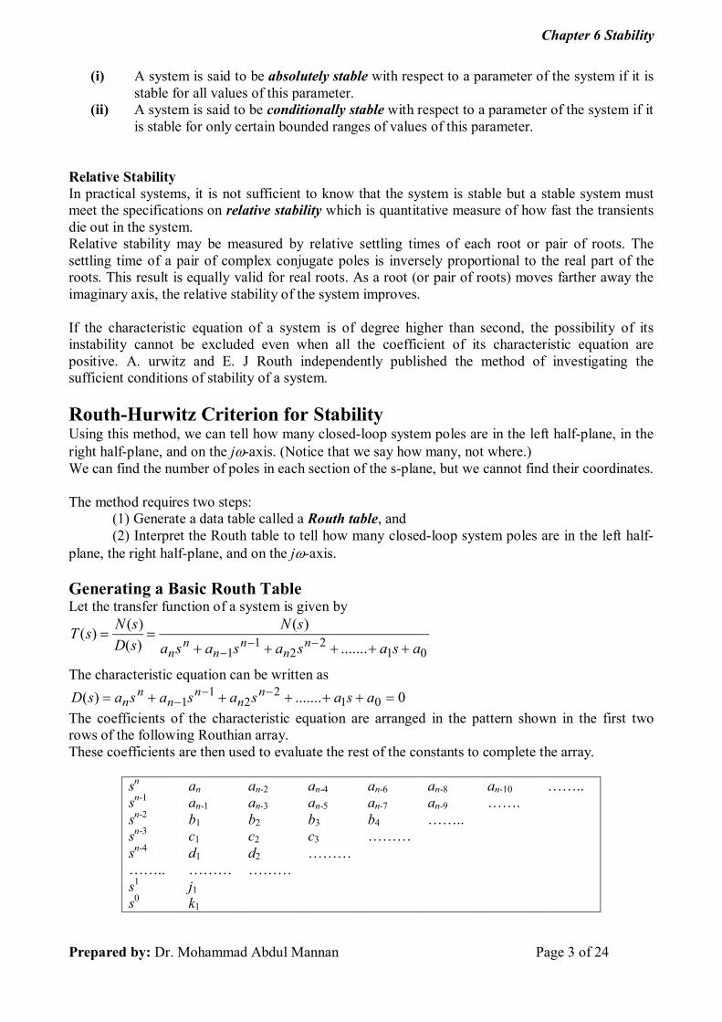
The coefficients of the characteristic equation are arranged in the pattern shown in the first two rows of the following Routhian array. These coefficients are then used to evaluate the rest of the constants to complete the array.

sn an an-2 an-4 an-6 an-8 an-10 …….. sn-1 an-1 an-3 an-5 an-7 an-9 ……. sn-2 b1 b2 b3 b4 …….. sn-3 c1 c2 c3 ……… sn-4 d1 d2 ……… …….. ……… ……… s1 j1 s0 k1

Chapter 6 Stability


The constants b1, b2, b3, b4, etc., in the third row are evaluated as follows:

1

3211

n

nnnn

a

aaaab

1

5412

n

nnnn

a

aaaab

1

7613

n

nnnn

a

aaaab

1

9814

n

nnnn

a

aaaab

This pattern is continued until the rest of the b’s are all equal to zero. Then the c row is formed by using the sn-1 and sn-2 rows. The constants c1, c2, c3, etc., in the third row are evaluated as follows:

1

21311

b

baabc nn

1

31512

b

baabc nn

1

41713

b

baabc nn

This pattern is continued until the rest of the c’s are all equal to zero. Then the d row is formed by using the sn-2 and sn3 rows. The constants d1, d2, etc., in the third row are evaluated as follows:

1

21211

c

cbbcd

1

31312

c

cbbcd

This process is continued until no more d terms are present. The rest of the rows are formed in this way down to the s0 row. The complete array is triangular, ending with the s0 row. Notice that the s1

and s0 rows contain only one term each.

Interpreting the Basic Routh Table (Routh-Hurwitz Criterion) The necessary and sufficient condition for system to be stable is “All the terms in the first column of Routh’s array must have same sign. There should not be any sign change in the first column of Routh’s array.” If there are any big changes existing then,

(a) System is unstable (b) The number of sign changes equals the number of roots lying in the right half of the s-plane.

The Routh-Hurwitz criterion declares that the number of roots of the polynomial that are in the right half-plane is equal to the number of sign changes in the first column.

Example 6.1.1 02401527210)( 2345 ssssssD

The Routhian array is formed by using the procedure described above:

s5: 1 10 152 s4: 1 72 240 s3: -62 -88 s2: 70.6 240 s1: 122.6 s0: 240

In the first column there are two changes of sign, from1 to - 62 and from – 62 to 70.6; therefore, Q(s) has two roots in the right-half s plane (RHP). This criterion gives the number of roots with positive real parts but does not tell the values of the roots. If Eq. (6.9) is factored, the roots are s1=-3, s2,3 = 1 j 3,and s4,5= 2j4. This calculation confirms that there are two roots with positive real parts. The Routh criterion does not distinguish between real and complex roots.

Chapter 6 Stability


Theorem 1: Division of a Row The coefficients of any row may be multiplied or divided by a positive number without changing the signs of the first column. The labor of evaluating the coefficients in Routh’s array can be reduced by multiplying or dividing any row by a constant. This may result, for example, in reducing the size of the coefficients and therefore simplifying the evaluation of the remaining coefficients. The following example illustrates this theorem:

20125923)( 23456 sssssssD

The Routhian array is

s6 1 2 5 20 s5 3 9 12 1 3 4 (After dividing by 3) s4 -1 1 20 s3 4 24 1 6 (After dividing by 4) s2 7 20 s1 22/7 22 (After multiplying by 7) s0 20

Notice that the size of the numbers has been reduced by dividing the s5 row by 3 and the s3 row by 4. The result is unchanged; i.e., there are two changes of signs in the first column and, therefore, there are two roots with positive real parts. Example 6.1: Make the Routh table for the system shown in Figure 6.4(a).

FIGURE 6.4 (a) Feedback system for Example 6.1; (b) equivalent closed-loop system.

Solution: The transfer function of feedback system is

10303110

1000)(

23

ssssT

The characteristic equation is

010303110)( 23 ssssD

The Routh array for this equation is given in Table 6.3.

Chapter 6 Stability


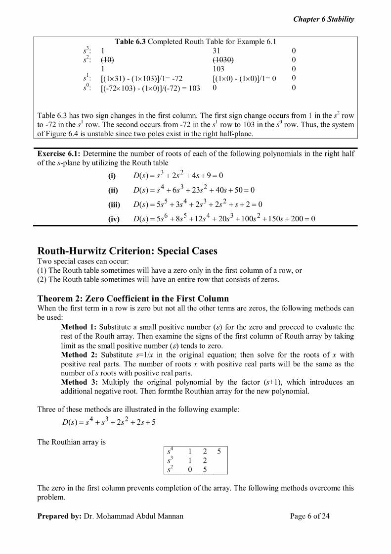
Table 6.3 Completed Routh Table for Example 6.1 s3: 1 31 0 s2: (10) (1030) 0 1 103 0 s1: [(131) - (1103)]/1= -72 [(10) - (10)]/1= 0 0 s0: [(-72103) - (10)]/(-72) = 103 0 0

Table 6.3 has two sign changes in the first column. The first sign change occurs from 1 in the s2 row to -72 in the s1 row. The second occurs from -72 in the s1 row to 103 in the s0 row. Thus, the system of Figure 6.4 is unstable since two poles exist in the right half-plane.

Exercise 6.1: Determine the number of roots of each of the following polynomials in the right half of the s-plane by utilizing the Routh table

(i) 0942)( 23 ssssD

(ii) 05040236)( 234 sssssD

(iii) 022235)( 2345 ssssssD

(iv) 0200150100201285)( 23456 sssssssD

Routh-Hurwitz Criterion: Special Cases Two special cases can occur: (1) The Routh table sometimes will have a zero only in the first column of a row, or (2) The Routh table sometimes will have an entire row that consists of zeros.

Theorem 2: Zero Coefficient in the First Column When the first term in a row is zero but not all the other terms are zeros, the following methods can be used:

Method 1: Substitute a small positive number () for the zero and proceed to evaluate the rest of the Routh array. Then examine the signs of the first column of Routh array by taking limit as the small positive number () tends to zero. Method 2: Substitute s=1/x in the original equation; then solve for the roots of x with positive real parts. The number of roots x with positive real parts will be the same as the number of s roots with positive real parts. Method 3: Multiply the original polynomial by the factor (s+1), which introduces an additional negative root. Then formthe Routhian array for the new polynomial.

Three of these methods are illustrated in the following example:

522)( 234 sssssD


s4 1 2 5 s3 1 2 s2 0 5

The zero in the first column prevents completion of the array. The following methods overcome this problem.

Chapter 6 Stability


METHOD 1: The Roth array is formed as shown below:

s4: 1 2 5 s3: 1 2 0 s2: (0) 5 0 s1: (2-5)/ 0 s0: 5

52lim

52lim

00

which is negative.

Hence, there are two sign changes in the first-column and so there are two roots of the equation Q(s) = 0 that lie in the right-half plane. The system represented by this characteristic equation is thus unstable.

METHOD 2: Letting s=1/x and rearranging the polynomial gives

1225)( 234 xxxxsD

The new Routhian array is

x4: 5 2 1 x3: 2 1 x2: -1 2 x1: 5 x0: 2

There are two changes of sign in the first column. Therefore, there are two roots of x in the RHP. The number of roots s with positive real parts is also two. This method does not work when the coefficients of Q(s) and of Q(x) are identical.

METHOD 3: 57432)(1)( 23451 ssssssDssD


s5 1 3 7 5 s4 2 4 s3 2 9 s2 -10 10 s1 11 s0 10

The same result is obtained by both methods. There are two changes of sign in the first column, so there are two zeros of Q(s) with positive real parts.

Chapter 6 Stability


Example 6.2 [Nise]: Determine the stability of the closed-loop transfer function

35632

10)(

2345

ssssssT

Method 1:

s5: 1 3 5 s4: 2 6 3 s3: (0) 7/2 0 s2:

76

3 0

s1:

1412

64942 2

0 0

s0: 3 0 0

76lim

76lim

00 , which is negative.

2

7

14

49

1412

64942lim

2

0

, which is positive.

There are two changes in sign in the first column of the Routh array, which tell us that there are two s-roots in the right half s-plane. Hence, the system is unstable having two poles in the right half s-plane. Method 2: Replacing s by 1/s in the characteristic equation and rearranging, we get

123653)( 2345 ssssssD

The Routh array for this equation is s5: 3 6 2 s4: 5 3 1 s3: 4.2 1.4 s2: 1.33 1 s1: -1.75 s0: 1

Since there are two sign changes, the system is unstable and has two right-half-plane poles. This is the same as the result obtained in Method 1. Notice that Table 6.6 does not have a zero in the first column. Example [Related to Theorem 2]: Consider the characteristic equation

05322 2345 sssss Solution: Method 1: The Routh array is

s5: 1 2 3 s4: 1 2 5 s3: (0) -2 0 s2:

22

5 0

Chapter 6 Stability


s1:

22

245 2

0

s0: 5

22lim

22lim

00 which is positive.

222

445lim

2

0

which is negative.

Examining the terms in the first column of the Routh array, it is found that there are two changes in sign and hence the system is unstable having two poles in the right half s-plane. Method 2: Replacing s by 1/s in the characteristic equation and rearranging, we get

012235 2345 sssss The Routh array for this equation is

s5: 5 2 1 s4: 3 2 1 s3: -4/3 -2/3 s2: 1/2 1 s1: 2 s0: 1

There are two changes in sign in the first column of the Routh array, which tell us that there are two s-roots in the right half s-plane. Hence, the system is unstable having two poles in the right half s-plane.

Method 3: 015322 2345 ssssss

053225322 234523456 sssssssssss

0585432 23456 ssssss

s6: 1 3 5 5 s5: (2) 1 (4) 2 (8) 4 0 s4: 1 1 5 0 s3: 1 -1 0 0 s2: 2 5 s1: -7 s0: 5


Or, 0112235 2345 ssssss

0122352235 234523456 sssssssssss

01234585 23456 ssssss

Chapter 6 Stability


s6: 5 5 3 1 s5: (8) 4 (4) 2 (2) 1 0 s4: 5/2 7/4 1 s3: -4/5 -3/5 0 0 s2: -1 1 s1: -7/5 0 s0: 1


Theorem 3: Entire Row is Zero (A Zero Row) When all the coefficients of one row are zero, the procedure is as follows:

1. The auxiliary equation can be formed from the preceding row, as shown below. 2. The Routhian array can be completed by replacing the all-zero row with the coefficients obtained by differentiating the auxiliary equation. 3. The roots of the auxiliary equation are also roots of the original equation. These roots occur in pairs and are the negative of each other. Therefore, these roots may be imaginary (complex conjugates) or real (one positive and one negative), may lie in quadruplets (two pairs of complex-conjugate roots), etc.

Consider the system that has the characteristic equation

1818112)( 234 sssssD

The Routhian array is s4: 1 11 18 s3: 2, 1 18, 9 s2: 2, 1 18, 9 s1: 0

The presence of a zero row (the s1 row) indicates that there are roots that are the negatives of each other. The next step is to form the auxiliary equation from the preceding row, which is the s2 row. The highest power of s is s2, and only even powers of s appear. Therefore, the auxililary equation is

9)( 2 ssP

The roots of this equation are

These are also roots of the original equation. The presence of imaginary roots indicates that the output includes a sinusoidally oscillating component.

To complete the Routhian array, the auxiliary equation is differentiated and is

02)(

sds

sdP

The coefficients of this equation are inserted in the s1 row, and the array is then completed:

Chapter 6 Stability


s4: 1 11 18 s3: 2, 1 18, 9 s2: 2, 1 18, 9 s1: 2 s0: 9

Since there are no changes of sign in the first column, there are no roots with positive real parts. Example: Determine the number of right-half-plane poles for the following sixth-order system with the characteristic equation

01616201282)( 23456 sssssssD

Solution: The Routh array is

s6: 1 8 20 16 s5: 2 12 16 0 1 6 8 0 s4: 2 12 16 0 1 6 8 0 s3: 0 0 0

Since the terms in the s3-row are all zero, the Routh’s test break down. Now the auxiliary polynomial is formed from the coefficient of the row s4, which is given by

86)( 24 sssP Next we differentiate the polynomial with respect to s and obtain

0124)( 3 ss

ds

sdP

The zeros in the s3-row are now replaced by the coefficient 4 and 12. The Routh array then becomes

s6: 1 8 20 16 s5: 2 12 16 1 6 8 s4: 2 12 16 1 6 8 s3: 4 12 1 3 s2: 3 8 s1: 1/3 s0: 8

We see that there is no change of sign in the first column of the new array. By solving for the roots of auxiliary polynomial

086 24 ss We find that the roots are

2js and 2js These two pairs of roots are also the roots of the original characteristic equation. Since there is no sig changes in the new array formed with the help of the auxiliary polynomial, we conclude that no root of characteristic equation has positive real part. Therefore, the system under consideration is limited stable.

Chapter 6 Stability


Example 6.4 [Nise]: Determine the number of right-half-plane poles in the closed-loop transfer function

5684267

10)(

2345

ssssssT

Solution: 5684267)( 2345 ssssssD


s5: 1 6 8 s4: 7 1 42 6 56 8 s3: 0 0 0

The s3 row is zero row. The auxililary equation is

86)( 24 sssP

Next we differentiate the polynomial with respect to s and obtain

0124)( 3 ss

ds

sdP


s5: 1 6 8 s4: 7 1 42 6 56 8 s3: 0 4 1 0 12 3 0 0 0 s2: 3 8 0 s1: 1/3 0 s0: 8

Table 6.7 shows that all entries in the first column are positive. Hence, there are no right–half-plane poles.

Chapter 6 Stability


Even Polynomial: The polynomial which has even power of s is called even polynomial. For example: s4+5s2+7 is a even polynomial. Odd Polynomial: The polynomial which has odd power of s is called odd polynomial. For example: s5+5s3+7s is an odd polynomial. Let us look further into the case that yields an entire row of zeros. An entire row of zeros will appear in the Routh table when a purely even or purely odd polynomial is a factor of the original polynomial. Even polynomials only have roots that are symmetrical about the origin. This symmetry can occur under three conditions of root position: (1) The roots are symmetrical and real, (2) The roots are symmetrical and imaginary, (3) The roots are quadrantal. Figure 6.5 shows examples of these cases. Each case or combination of these cases will generate an even polynomial. It is this even polynomial that causes the row of zeros to appear. Thus, the row of zeros tells us of the existence of an even polynomial whose roots are symmetric about the origin. Some of these roots could be on the j-axis. On the other hand, since j roots are symmetric about the origin, if we do not have a row of zeros, we cannot possibly have j roots.

Another characteristic of the Routh table for the case in question is that the row previous to the row of zeros contains the even polynomial that is a factor of the original polynomial. Finally, everything from the row containing the even polynomial down to the end of the Routh table is a test of only the even polynomial. Let us put these facts together in an example. The polynomial s5+5s3+7s is an example of an odd polynomial; it has only odd powers of s. Odd polynomials are the product of an even polynomial and an odd power of s. Thus, the constant term of an odd polynomial is always missing. Example 6.5: For the transfer function

20384859392212

20)(

2345678

sssssssssT (6.11)

tell how many poles are in the right half-plane, in the left half-plane, and on the j-axis. Solution:

20384859392212)( 2345678 sssssssssD

Chapter 6 Stability


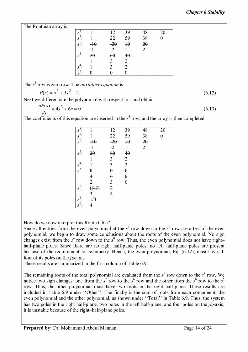
The Routhian array is s8: 1 12 39 48 20 s7: 1 22 59 38 0 s6: -10 -20 10 20 -1 -2 1 2 s5: 20 60 40 1 3 2 s4: 1 3 2 s3: 0 0 0

The s3 row is zero row. The auxililary equation is

23)( 24 sssP (6.12)

Next we differentiate the polynomial with respect to s and obtain

064)( 3 ss

ds

sdP (6.13)


s8: 1 12 39 48 20 s7: 1 22 59 38 0 s6: -10 -20 10 20 -1 -2 1 2 s5: 20 60 40 1 3 2 s4: 1 3 2 s3: 0 0 0 4 6 0 2 3 0 s2: (3/2) 2 3 4 s1: 1/3 s0: 4

How do we now interpret this Routh table? Since all entries from the even polynomial at the s4 row down to the s0 row are a test of the even polynomial, we begin to draw some conclusions about the roots of the even polynomial. No sign changes exist from the s4 row down to the s0 row. Thus, the even polynomial does not have right–half-plane poles. Since there are no right–half-plane poles, no left–half-plane poles are present because of the requirement for symmetry. Hence, the even polynomial, Eq. (6.12), must have all four of its poles on the j-axis. These results are summarized in the first column of Table 6.9. The remaining roots of the total polynomial are evaluated from the s8 row down to the s4 row. We notice two sign changes: one from the s7 row to the s6 row and the other from the s6 row to the s5 row. Thus, the other polynomial must have two roots in the right half-plane. These results are included in Table 6.9 under ‘‘Other’’. The finally is the sum of roots from each component, the even polynomial and the other polynomial, as shown under ‘‘Total’’ in Table 6.9. Thus, the system has two poles in the right half-plane, two poles in the left half-plane, and four poles on the j-axis; it is unstable because of the right–half-plane poles.

Chapter 6 Stability


Table 6.9 Summary of pole locations for Example 6.5

Polynomial

Even other Total Location (Fourth-order) (Fourth-order) (Eight-order)

Right half-plane 0 2 2 Left half-plane 0 2 2 On imaginary

(j) axis 4 0 4

Example 6.6 Find the number of poles in the left half-plane, the right half-plane, and on the j-axis for the system of Figure 6.6.

Solution: First, find the closed-loop transfer function as

The Routh table for the denominator of Eq. (6.14) is shown as Table 6.10. For clarity, we leave most zero cells blank. At the s1 row there is a negative coefficient; thus, there are two sign changes. The system is unstable, since it has two right–half-plane poles and two left–half-plane poles. The system cannot have j poles since a row of zeros did not appear in the Routh table.

Example 6.7: Find the number of poles in the left half-plane, the right half-plane, and on the j-axis for the system of Figure 6.7.

Solution: The closed-loop transfer function is

Chapter 6 Stability


Form the Routh table shown as Table 6.11, using the denominator of Eq. (6.15). A zero appears in the first column of the s3 row. Since the entire row is not zero, simply replace the zero with a small quantity, , and continue the table. Permitting to be a small, positive quantity, we find that the first term of the s2 row is negative. Thus, there are two sign changes, and the system is unstable, with two poles in the right half-plane. The remaining poles are in the left half-plane.

We also can use the alternative approach, where we produce a polynomial whose roots are the reciprocal of the original. Using the denominator of Eq. (6.15), we form a polynomial by writing the coefficients in reverse order,

The Routh table for this polynomial is shown as Table 6.12. Unfortunately, in this case we also produce a zero only in the first column at the s2 row. However, the table is easier to work with than Table 6.11. Table 6.12 yields the same results as Table 6.11: three poles in the left half-plane and two poles in the right half-plane. The system is unstable.

Example 6.8: Find the number of poles in the left half-plane, the right half-plane, and on the j-axis for the system of Figure 6.8. Draw conclusions about the stability of the closed-loop system.

Solution: The closed-loop transfer function for the system of Figure 6.8 is

Using the denominator, form the Routh table shown as Table 6.13. A row of zeros appears in the s5 row. Thus, the closed-loop transfer function denominator must have an even polynomial as a factor. Return to the s6 row and form the even polynomial:

Chapter 6 Stability


Differentiate this polynomial with respect to s to form the coefficients that will replace the row of zeros:

Replace the row of zeros at the s5 row by the coefficients of Eq. (6.19) and multiply through by 1/2 for convenience. Then complete the table. We note that there are two sign changes from the even polynomial at the s6 row down to the end of the table. Hence, the even polynomial has two right–half- plane poles. Because of the symmetry about the origin, the even polynomial must have an equal number of left–half-plane poles. Therefore, the even polynomial has two left–half-plane poles. Since the even polynomial is of sixth order, the two remaining poles must be on the j-axis. There are no sign changes from the beginning of the table down to the even polynomial at the s6 row. Therefore, the rest of the polynomial has no right–half-plane poles. The results are summarized in Table 6.14. The system has two poles in the right half-plane, four poles in the left half-plane, and two poles on the j-axis, which are of unit multiplicity. The closed-loop system is unstable because of the right–half-plane poles.

Chapter 6 Stability


Exercise 6.2: Tell how many roots of the following polynomial are in the right half-plane, in the left half-plane, and on the j-axis by utilizing the Routh table:

(i) 081263)( 234 sssssD

(ii) 015322)( 2345 ssssssD

(iii) 03453)( 2345 ssssssD

(iv) 02344)( 2345 ssssssD

(v) 042632)( 2345 ssssssD

(vi) 048422)( 23456 ssssssssD

Exercise 6.3: For the following systems, tell how many closed-loop poles are located in the right half-plane, in the left half-plane, and on the j-axis.

System 1

System 2

System 3

Example 6.9: Find the range of gain, K, for the system of Figure 6.10 that will cause the system to be stable, unstable, and marginally stable. Assume K > 0.

Solution: First find the closed-loop transfer function as

Next form the Routh table shown as Table 6.15.

Chapter 6 Stability


Since K is assumed positive, we see that all elements in the first column are always positive except the s1 row. This entry can be positive, zero, or negative, depending upon the value of K. If K < 1386, all terms in the first column will be positive, and since there are no sign changes, the system will have three poles in the left half-plane and be stable. If K > 1386, the s1 term in the first column is negative. There are two sign changes, indicating that the system has two right–half-plane poles and one left– half-plane pole, which makes the system unstable. If K = 1386, we have an entire row of zeros, which could signify j poles. Returning to the s2 row and replacing K with 1386, we form the even polynomial

Differentiating with respect to s, we have

Replacing the row of zeros with the coefficients of Eq. (6.22), we obtain the Routh-Hurwitz table shown as Table 6.16 for the case of K = 1386.

Since there are no sign changes from the even polynomial (s2 row) down to the bottom of the table, the even polynomial has its two roots on the j-axis of unit multiplicity. Since there are no sign changes above the even polynomial, the remaining root is in the left half-plane. Therefore the system is marginally stable. Example 6.10: Factor the polynomial

Solution: Form the Routh table of Table 6.17. We find that the s1 row is a row of zeros. Now form the even polynomial at the s2 row:

This polynomial is differentiated with respect to s in order to complete the Routh table. However, since this polynomial is a factor of the original polynomial in Eq. (6.23), dividing Eq. (6.23) by (6.24) yields (s2+3s+20) as the other factor. Hence,

Chapter 6 Stability


Example 6.5 [Control Systems Egineering, By I. J. Nagrath]: A unity negative feedback control system has an open-loop transfer function consisting of two poles, two zeros and a variable gain K. The zeros are located at – 2 and -1; and the poles at 0.1 and +1. Using Routh stability criterion, determine the range of values of K for which the closed-loop system has 0, 1, or 2 poles in the right-half s-plane.

Solution: )1)(1.0(

)2)(1()(

ss

ssKsG

The characteristic equation of the system is given as

0)2)(1()1)(1.0()(1)( ssKsssGsD

0)1.02()9.03()1()( 2 KsKsKsD

s2: (1+K) (2K-0.1) s1: (3K-0.9) 0 s0: (2K-0.1) 0

(i) No poles in right half s-plane (system stable)

1+K >0 K > - 1 3K-0.9 > 0 K > 0.3 2K-0.1 >0 K > 0.05

Hence, K > 3. (ii) One pole in right half s-plane (=one change of sign in first column terms)

-1<K<0.05 (iii) Two poles in right half s-plane (= two changes of sign in first column terms)

0.05<K<0.3 Example 5.6 Let us determine the range of K, adjustable loop gain, for the system described by the following characteristic equation to be: (a) Stable; (b) Unstable, and (c) Limitedly (conditionally) stable.

08)( 23 KssssD

Solution: The Routh array is:

Chapter 6 Stability


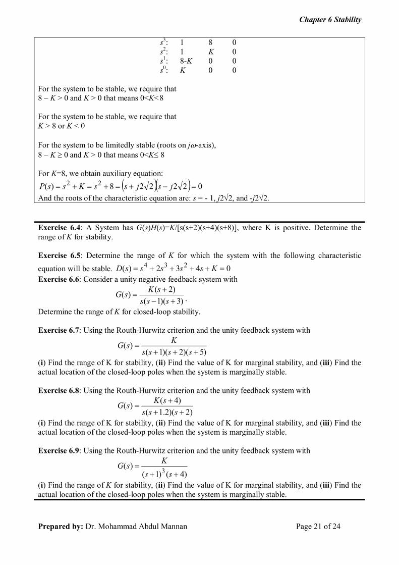
s3: 1 8 0 s2: 1 K 0 s1: 8-K 0 0 s0: K 0 0

For the system to be stable, we require that 8 – K > 0 and K > 0 that means 0<K<8 For the system to be stable, we require that K > 8 or K < 0 For the system to be limitedly stable (roots on j-axis), 8 – K 0 and K > 0 that means 0<K 8 For K=8, we obtain auxiliary equation:

022228)( 22 jsjssKssP

And the roots of the characteristic equation are: s = - 1, j22, and -j22.

Exercise 6.4: A System has G(s)H(s)=K/[s(s+2)(s+4)(s+8)], where K is positive. Determine the range of K for stability. Exercise 6.5: Determine the range of K for which the system with the following characteristic

equation will be stable. 0432)( 234 KsssssD Exercise 6.6: Consider a unity negative feedback system with

)3)(1(

)2()(

sss

sKsG .

Determine the range of K for closed-loop stability. Exercise 6.7: Using the Routh-Hurwitz criterion and the unity feedback system with

)5)(2)(1()(

ssss

KsG

(i) Find the range of K for stability, (ii) Find the value of K for marginal stability, and (iii) Find the actual location of the closed-loop poles when the system is marginally stable. Exercise 6.8: Using the Routh-Hurwitz criterion and the unity feedback system with

)2)(2.1(

)4()(

sss

sKsG

(i) Find the range of K for stability, (ii) Find the value of K for marginal stability, and (iii) Find the actual location of the closed-loop poles when the system is marginally stable. Exercise 6.9: Using the Routh-Hurwitz criterion and the unity feedback system with

)4()1(

)(3

ss

KsG

(i) Find the range of K for stability, (ii) Find the value of K for marginal stability, and (iii) Find the actual location of the closed-loop poles when the system is marginally stable.

Chapter 6 Stability


Marginal K and Frequency of Sustained Oscillations Marginal value of gain ‘K’ is that value of gain ‘K’ for which system becomes marginally stable. For marginally stable system there are must be a row of zeros occurring in Routh’s array. So the value of gain ‘K’ which makes any row of Routh array as row of zero is called marginal value of gain ‘K’. Now K = 0 makes row of s0 as row of zeros but K = 0 cannot be marginal value, because for K = 0, constant term in the characteristic equation becomes zero i.e. one coefficient for s0 vanishes which makes system unstable instead of marginally stable. Hence, marginal value of gain ‘K’ is a value which makes any row other than s0 as row of zero. To obtain the frequency of oscillations, solve the auxiliary equation P(s) =0 for K = Kmar. The magnitude of imaginary roots of P(s) = 0 obtained for marginal value of gain K (Kmar) indicates the frequency of sustained oscillations, which system is going to produce. The gain margin is the factor by which the given value of K can be multiplied to get the marginal value of K. If Kmar is the marginal value of K, then the gain margin is,

K

K

K

KGM mar

ofvalueSpecified

ofvalueMarginal

Example 6.15: For unity feedback system, )25.01)(4.01(

)(sss

KsG

, find (i) the range of

values of K, (ii) the marginal value of K, and (iii) the frequency of sustained oscillations. Solution: (i) Characteristic equation 1+G(s)H(s)=0 and here H(s)=1, thus we have

0)25.01)(4.01( Ksss

0)165.01.0( 2 Ksss

065.01.0 23 Ksss The Routh array

s3: 0.1 1 0 s2: 0.65 K 0 s1:

65.0

1.065.0 K

0 0

s0: K 0 0 From s0: K>0 From s1: 0.65-0.1K>0 K<6.5 Thus Range of value of K, 0<K<6.5. (ii) The marginal value of ‘K’ is a value which makes any row other than s0 as row of zeros. Thus,

0.65-0.1Kmar = 0 So, Kmar = 6.5

(iii) To find frequency, find out roots of auxiliary equation at marginal value of ‘K’.

P(s) = 0.65s2+Kmar = 0.65s2+ 6.5 = 0 s2 = -10 s = j3162

Comparing with s = j = frequency of oscillations = 3.162 rad/sec.

Chapter 6 Stability


Stability in State Space At first the characteristics equation is derived from the state equation then apply the Routh-Hurwitz Criterion. Example 6.11: Given the system

Solution: First form (sI – A):

Now find the det(sI – A):

Using this polynomial, form the Routh table of Table 6.18.

Since there is one sign change in the first column, the system has one right–half-plane pole and two left–half-plane poles. It is therefore unstable. Yet, you may question the possibility that if a nonminimum-phase zero cancels the unstable pole, the system will be stable. However, in practice, the nonminimum-phase zero or unstable pole will shift due to a slight change in the system’s parameters. This change will cause the system to become unstable.

Chapter 6 Stability


Exercise 6.10: A system is represented in state space as

u

0

1

0

341

422

310

xx ; x011y

Determine how many eigenvalues are in the right half-plane, in the left half-plane, and on the j-axis. Exercise 6.11: The following system in state space represents the forward path of a unity feedback system. Use the Routh-Hurwitz criterion to determine if the closed-loop system is stable.

u

-

1

0

0

543

310

010

xx ; x110y

Advantages of Routh’s Criterion Stability of the system can be judge without actually solving the characteristic equation. No evaluation of determinants, which saves calculation time. For unstable system it gives number of roots of characteristic equation having positive real

part. Relative stability of the system can be easily judge. It helps I finding out range of value of gain ‘K’ for system stability. It helps in finding out intersection points of root locus with imaginary axis. By using this criterion, critical value of system gain can be determined hence frequency of

sustained oscillation s can be determined.

Limitation or Disadvantage of Routh’s Criterion It is valid for real coefficient of the characteristic equation. It does not provide exact of the closed loop poles in left or right half of s-plane. It does not suggest methods of stabilizing an unstable system Applicable only to linear systems.

References

[1] Norman S. Nise, “Control Systems Engineering,” Sixth Edition, John Wiley and Sons, Inc, 2011.

Documents

Stability - · A system is unstable if any bounded input yields an unbounded output. 3. A system is marginal or limitedly or critically stability means the system is stable for some