Stability of supported vertical cuts in granular matters ...scientiairanica.sharif.edu/article_2416_58043afd9c4ccfaf6119f3a... · Stability of supported vertical cuts in granular

Scientia Iranica A (2017) 24(2), 537{550

Sharif University of TechnologyScientia Iranica

Transactions A: Civil Engineeringwww.scientiairanica.com

Stability of supported vertical cuts in granular mattersin presence of the seepage ow by a semi-analyticalapproach

M. Veiskaramia,b;� and S. Fadaieb

a. School of Engineering, Shiraz University, Shiraz, Iran.b. Faculty of Engineering, University of Guilan, Rasht, Iran.

Received 31 October 2015; received in revised form 1 December 2015; accepted 18 June 2016

KEYWORDSStability;Complex analysis;Stress characteristics;Seepage;Granular matter.

Abstract. Vertical cuts are prone to several types of failure such as piping, groundheaving, and deep-seated or base failure. The latter is the subject of this study andprobably attracts less attention in comparison to other types of failure. Although it iscommonly believed that such a failure is rare in normal conditions; in presence of theseepage ow, deep-seated failure is much likely to initiate and advance prior to other typesof failure. In this paper, the stability analysis of vertical cuts in granular soils in presenceof the seepage ow is studied against the deep failure. To do so, the stability analysis ismade by the use of the well-known method of stress characteristics with inclusion of theseepage ow force. This nonuniform ow �eld renders the stability analysis quite complex.A semi-analytical approach, based on complex algebra, is presented to �nd the ow �eld,which is accurate and much faster for calculation of the seepage force at arbitrary points inthe �eld. The solution of the ow �eld is a background solution for the stress �eld whichis to be found to assess the stability.

© 2017 Sharif University of Technology. All rights reserved.

1. Introduction

Stability problems in soil mechanics may be stemmedfrom historical contributions of Coulomb (1776) andRankine (1857) including the slope stability, bearingcapacity, and lateral earth pressure problems as clas-sical problems [1,2]. For stability analysis of verticalcuts, some of such problems are involved and should bechecked. In this regard, according to Terzaghi (1943),two major types of failure of vertical cuts are theslope failure and the base (or deep-seated) failure [3].As vertical cuts in granular soils are often supported

*. Corresponding author. Tel.: +98 71 36133102;Fax: +98 71 36473161E-mail addresses: [email protected] (M.Veiskarami); [email protected] (S. Fadaie)

by either exible or rigid retaining structures, the�rst kind of failure, i.e. the slope failure, is seldom aproblem; instead, conventional approaches are focusedon the estimation of the lateral earth pressure and/orstability against the deep-seated failure. In many cases,vertical cuts are excavated below the groundwater tableor adjacent to rivers or banks. As a result, there willbe another type of failure beside the slope or the basefailure, which is attributed to the piping or groundheaving due to the seepage ow.

The literature review behind the stability analysisfor problems addressed above is rather long and richwith contributions including the force limit equilibriummethods (classically Coulomb, 1776; more recently Ku-mar and Subba Rao, 1997; Subba Rao and Choudhury,2005; Barros, 2006; Ghosh, 2008; Ghosh and Sharma,2012; Barros and Santos, 2012; Ling et al., 2014) [1,4-

538 M. Veiskarami and S. Fadaie/Scientia Iranica, Transactions A: Civil Engineering 24 (2017) 537{550

10], method of stress characteristics (Sokolovskii, 1965;Larkin, 1968; Sabzevari and Ghahramani, 1972 and1973; Houlsby and Wroth, 1982; Kumar, 2001; Kumarand Chitikela, 2002) [11-17] or the limit analysis (Chen,1969; Lysmer, 1970; Chen and Davidson, 1973; Collins,1973; Chen, 1975; Arai and Jinki, 1990; Soubra,2000; Soubra and Macuh, 2002; Shiau et al., 2008;Jahanandish et al., 2010; Veiskarami et al., 2014) [18-28], among others. Attempts to include the e�ect ofthe groundwater ow in the stability analysis may dateback to Terzaghi (1943) who studied the stability of thesoil mass in the vicinity of sheet pile walls [3]. Manysimilar problems have been studied so far which includethe e�ect of the groundwater ow on the bearingcapacity and the earth pressure on retaining walls [9,29-31]. In 1999, Soubra and his coworkers studied theimportant problem of the passive earth pressure onsheet pile walls subjected to the seepage ow andassociated hydraulic gradients [32]. In this regard,Barros (2006) [6], Benmebarek et al. (2006) [33],Barros and Santos (2012) [9] and most lately, Santosand Barros (2015) [34] investigated active and passiveearth pressures problems in presence of the seepage.Recently, Veiskarami and Zanj (2014) made an attemptto include the seepage force in the stress characteristicsequations and compute the passive earth pressure onsheet pile walls subjected to the groundwater ow [35].They employed the �nite element technique to solvethe ow �eld as a background solution which isassumed to remain unin uenced by the stress �eldat the limiting equilibrium. The background �niteelement mesh was then used to interpolate the seepageforce through the stress �eld at the limiting equilib-rium.

Although evidence indicated that both the bear-ing capacity and earth pressure problems in presenceof the seepage ow are investigated by researchers,no attempt is known to the authors dealing with theparticular problem of the deep-seated failure adjacentto the supported vertical cuts. In this research, thisis the matter of focus. The stability analysis involvescomplexities due to the complex form of the seepage ow behind vertical cuts. The general methodology toinvestigate this problem is based on the assumptionsmade by Veiskarami and Zanj (2014) [35] who formallyassumed that the seepage ow �eld is only a functionof the geometry of the problem domain and does notchange with the formation of the failure mechanism atthe limiting state. Therefore, the solution of the ow�eld can be found independent of the solution of thestress �eld. Moreover, an analytical solution of the ow �eld will be presented which obviates any furtherneed for numerical solutions like that of Veiskaramiand Zanj (2014) [35]. What comes next comprises thestatement of the problem, �eld equations, and solutiontechniques.

2. Statement of the problem

A vertical cut in a granular matter cannot be ad-vanced without a lateral support. Such supports areoften provided with exible walls with a series ofstruts and wales as a bracing system, internal groundanchor supports, mechanically stabilized soil systemwith facing elements, facing elements, and externalsupports or other systems [36,37]. Figure 1 shows anumber of techniques which can be applied to low-depth and deep excavations. For excavations wherethe height of the wall is small, a cantilever sheet pilecan be used with additional depth extended into theground to provide the required exural sti�ness whichis schematically depicted in Figure 1(a). Such wallscan be enhanced with ground anchor (Figure 1(b))to increase their sti�ness and reduce their de ectionand lateral displacement. For deep excavations, sheetpile walls must be internally or externally supportedas illustrated in Figure 1(c) and (d). In stagedconstruction, as the excavation advances into theground, facing elements, often consisting of a weldedwire mesh faced with shotcrete, steel sheets, etc., areinstalled at each stage. The wall (facing) is sequentiallysupported by external or internal support system.This is schematically shown in Figure 1(e) and (f).Unlike the cantilever retaining walls, in many cases,the wall is not extended into the ground in other soilsupporting and wall construction techniques, or theextension length can be ignored in comparison to thewall height or due to its exibility. Therefore, it willbe of particular importance to analyze the stability ofsuch systems against a deep-seated (bearing capacity)failure, especially when the seepage ow exists towardsthe bottom of the cut.

Figure 1(g) schematically represents the simpli-�ed problem (a braced or supported excavation in thevicinity of a bank or a river) which coincides with mostcases where the excavation is performed with sheetpile walls or facing elements. In this problem, theexistence of the seepage ow should be paid specialattention. The seepage ow towards the bottom of thecut is a serious problem as it causes the increase in thelateral earth pressure on the supporting system andmay lead to piping or heaving failures. In addition, thedeep-seated or the bearing capacity failure becomes aserious problem as the seepage force not only multipliesthe actuating downward forces, but it also reduces themobilized strength in the passive zone beneath thebottom of the cut.

Figure 1(h) illustrates the statement of the prob-lem which is investigated theoretically. In this �gure,the formation of a failure mechanism in terms of adeep-seated (or bearing capacity) problem is presentedwithin a shaded area BCDQ. This area contains amass of soil, which is assumed to be at plastic limiting

M. Veiskarami and S. Fadaie/Scientia Iranica, Transactions A: Civil Engineering 24 (2017) 537{550 539

Figure 1. Supported excavations in granular soil: (a) Low-depth excavation with cantilever sheet pile wall, (b) low-depthexcavation with cantilever sheet pile wall and internal support, (c) deep excavation with internal supports (ground anchor)and exible sheet pile wall, (d) deep excavation with external support system (struts), (e) deep excavation with facingunits, internally reinforced soil and staged construction, (f) deep excavation with facing units, external support system,and staged construction, (g) simpli�ed and idealized problem, and (h) statement of the solved problem.

equilibrium. The seepage force with a downwarddirection behind the wall increases the unbalancingforce in ABQP soil block. On the other hand, itis evident that the seepage ow in the plastic regioncauses a reduction in the resistance against deep-seatedfailure. Therefore, the problem that should be analyzedis similar to a bearing capacity problem involving

a seepage force �eld, for which there is no simplesolution.

To analyze this problem, one should determinethe ability of soil to withstand the unbalancing forcewhich is received from both the submerged weight ofthe soil in ABQP region intensi�ed by a downwardseepage ow force. Moreover, the existence of the


seepage ow in the plastic region causes a rathercomplex problem which is required to be solved to �nda factor of safety. In this regard, according to Terzaghi(1943) [3], the failure is caused by the weight of thesoil block within ABQP region. In addition to the shearresistance within the plastic region BCDQ, some lateralshear resistance is mobilized along the nearly verticalside AB (which is proportional to lateral earth pressure,PA). One should note that the exible nature of thewall and its lateral de ections permit mobilization ofany signi�cant shear resistance at the interface of thesoil block ABQP and the equivalent footing BQ atits base. This is also stated by Terzaghi (1943) [3].Moreover, the lateral earth pressure can be assumed toobey the active condition. Therefore, the global factorof safety against deep-seated failure, as also expressedby Terzaghi (1943) [3], can be de�ned as follows:

FS=Sum of resisting forcesSum of driving forces

=Qult

W 0ABQP+Ffd�S ; (1)

where Fs is the factor of safety against deep-seatedfailure, W 0ABQB is the submerged weight of soil block,ABQP, Ffd is the downward seepage ow force throughthe soil block ABQP, S is the lateral shear resistanceacting along boundary AB, and Qult is the capacityof the equivalent footing BQ at the bottom of the soilblock, ABQP. The ultimate pressure tolerable by thesoil mass can be reasonably computed by conventionalbearing capacity equation for a surface footing on agranular material as follows:

Qult = f 0B02N : (2)

In this equation, 0 is the submerged unit weight ofthe soil, B0 is the width of the equivalent footing (BQ,yet unknown), N is the third bearing capacity factorwhich includes the e�ect of weight, and f is a correc-tion factor which accounts for the e�ect of the seepage ow and is equal to unity when the seepage ow doesnot exist. This correction factor has been presented byKumar and Chakraborty (2012) [30] or Veiskarami andHabibagahi (2013) [38] for a horizontal seepage ow orby Veiskarami and Kumar (2013) [31] for inclined ow.However, for this very complex form of the seepage ow, there is no such factor available. Fortunately, aparticular procedure may involve direct solution to theproblem described above without requiring the bearingcapacity factor, N , and the correction factor, f , tobe computed separately. In the procedure presented inthis research, the ultimate resistance, Qult, is computeddirectly which automatically contains the e�ect of theseepage ow force. In essence, the factor of safety,Fs, will be the direct outcome of this research whichinvolves all necessary and still unde�ned parameterslike the pattern and intensity of the seepage ow, thewidth of the equivalent footing, B0, and so on.

As stated earlier, one should notice that in spiteof possible extension of the sheet pile deeper into theground, deep-seated failure would still be possible assuch a exible wall may not be able to properly providea lateral sti�ness and/or su�cient embedment depthagainst the plastically deforming mass. Therefore, thecase under study can be regarded as the critical casewhich can be applied to cases with or without extensionof the sheet pile into the ground. Therefore, as the mostcritical case, such an extended depth (if it probablyexists) is ignored.

3. Solution of the ow �eld

The statement of the ow problem can be easilyunderstood with regard to Figure 1. This is mathemat-ically equivalent to a mixed Dirichlet-Neumann typeproblem where either the potential head or the uxis prescribed along di�erent boundaries. For instance,the bedrock or any impervious layer is assumed to bereasonably deep into the soil. Thus, the statement ofthe problem can be mathematically expressed as a owproblem through a \degenerated" semi-in�nite domainconsisting of three di�erent boundaries: (i) along theboundary P0P, i.e. from minus in�nity to the top of thewall, the potential head or the water head is prescribed,i.e., it is equal to Hw, and hence, this is a Dirichlet-type boundary condition; (ii) along the boundary PQ,i.e. along the wall, there is no ux which is equivalentto a Neumann-type boundary condition; (iii) along theboundary QQ0, i.e. from the bottom of the cut to theplus in�nity, the water head is zero (datum) and again,a Dirichlet boundary condition exists. The steady-state ow equation can be expressed as follows:

r2h = 0; (3)

where h = h(x; y) is the water head at arbitrarypoint within the problem domain as the main �eldvariable and r2 (or equivalentlyr:r) is the Laplacianoperator.

For this problem, di�erent solutions exist [34,39-43]. Basic elements for the analytical solution can beseparately found in text books on complex analysis andalso in Harr (1962) [39]. Here, we present only theimportant details.

The ingredients of computational procedures areto �nd a solution to the Laplace equation (governingequation to the steady state ow) for a simple domainwith a known solution in terms of a complex function,and then transforming the domain, the solution andthe gradient of the solution into the domain of interest(main problem domain). To show the procedure, thesteady-state ow problem in a semi-in�nite plane withDirichlet and Neumann boundary conditions is pre-scribed along the boundaries, as shown in Figure 2(a).Note that the problem is de�ned in the complex plane.


Figure 2. Problem domains: (a) Upper half-plane and(b) main problem domain (transformed).

The boundary conditions are comprised of a con-stant unit hydraulic head distributed along the semi-in�nite line from �1 to -1 (Dirichlet type); isolatedline segment from -1 to +1 (Neumann type); and aconstant zero hydraulic head from +1 to +1 (Dirichlettype). Therefore, the solution function, h(z) = h(x; y),can be mathematically expressed as follows:

r2h = 0: (4a)

Subject to:8>>><>>>:h = 1 from �1 to � 1

h = 0 from + 1 to +1rh:ey = @h

@y = 0 from � 1 to + 1

(4b)

where ey is the unit base vector along the y-axis ornormal to the x-axis.

This is now necessary to �nd the solution in theupper half plane, and then transform it to the mainproblem domain shown in Figure 2(b). To handlethis problem and others like this, it is convenientto employ the conformal mapping technique of thecomplex algebra. A mapping in complex plane, w =f(z), is said to be conformal at some arbitrary point,zc, if it is both analytic and its derivative is nonzero atthat point:

f 0(zc) 6= 0: (5)

One important property of conformal mapping is thatit transforms orthogonal curves into orthogonal curves.This is useful when the steady-state seepage ow is

studied. Another important property of such transfor-mations is their ability in the transformation of func-tions satisfying the Laplace equation. Such functionsare real valued functions of z = x + iy and known asharmonic functions which possess continuously the �rstand second partial derivatives and satisfy the Laplaceequation. An important theorem in complex analysisstates that if an analytic function (f(z)) transformssome domain (Dz) in the z-plane onto another one(Dw) in the w-plane, then if a function hw (w) =hw(u; v) is harmonic in Dw, the function hD(z) =hD(x; y) = hw (u(x; y); v(x; y)) will be also harmonicin Dz [44]. This enables the application of conformalmapping in solution of Laplace equation in all domainsobtained by conformal mapping. To further advancethis problem, the solution to the Laplace equationin the upper half-plane is sought �rst, and then itwill be extended to the domain of interest. To doso, consider the semi-in�nite strip in w3-plane, shownin Figure 3(a), with its base isolated and its sidesinvolving Dirichlet boundary conditions as follows:8>>><>>>:

h = 1 from 0 to + i1h = 0 from �=2 to 1 + i1rh:ev3 = @h

@v3= 0 from 0 to �=2

(6)

where w3 = u3 + iv3, and e(v3) is the unit base vectornormal to u3-axis and h = h(w3). The completesolution to this problem, e.g. by inspection, can besimply expressed as the following unique closed-formsolution satisfying both the equation and boundaryconditions in w3-plane:

h(u3; v3) = 1� 2�u3; (7)

Now, a series of successive transformations will providethe solution in the upper half-plane of the complexplane, i.e. in z-plane. With reference to Figure 3(a)through (d), these transformations will eventually leadto the transformation of both the geometry and thesolution onto the complex z-plane.

Appendix A represents all successive transforma-tions with details found in texts on complex analy-sis [44,45]. Note that in all these equations wk =

Figure 3. The problem domain under di�erent transformations in complex plane.


uk + ivk, where k denotes any of the kth planes withinwhich a solution is sought. Therefore, the solution ofthe problem can be transformed to the upper half-planein the complex z-plane as follows (see Appendices):

h(u3; v3) = h(u3) = h (u3(u2; v2))

= h (u3 (u2(u1; v1); v2(u1; v1))) = :::

= h (u3(x; y)) ; (8)

or equivalently:

h(x; y) =1� 2�

sin�1�q

(u2(x; y) + 1)2 + v2(x; y)2

�q

(u2(x; y)� 1)2 + v2(x; y)2�:

(9)

Finally, the solution in the main problem domaincan be found by the following appropriate conformalmapping from the z-plane onto w-plane (Churchill etal. 1974) [44]:

w(z) =Hs

�

hp(z2 � 1) + cosh�1 z

i: (10)

One should notice that this function is a double-valuedcomplex function, owing to the presence of the squareroot term. To make a proper transform, it is vital tochoose a suitable branch cut. To do so, the argumentof z � 1 can be restricted to [0; 2�] and the argumentof z + 1 can be restricted to [��; �]. In this way,the function will become a single-valued function alongthe line segment [�1;+1]. These branch cuts are alsoshown in Figure 2(a) by two dashed lines extended fromthese two points towards �1.

Note that the solution is obtained for a unithydraulic head di�erence between the upstream andthe downstream. Since the Laplacian operator is linear(also homogeneous), this normalized solution can bemultiplied by Hw to obtain the solution for any actualcondition.

As it is necessary to �nd the gradient of thehydraulic head, rh, in the w-plane to calculate theseepage ow force, this can be achieved by making useof the chain rule in partial derivatives of a functionwhich requires the geometrical properties of the trans-formation of the problem domain from the z-plane ontothe w-plane by the Jacobian of the transform:8<:@w

@x = @w@u

@u@x + @w

@v@v@x

@w@y = @w

@u@u@y + @w

@v@v@y

)�@w@x@w@y

�=�@u@x

@v@x

@u@y

@v@y

��@w@u@w@v

�= [J ]

�@w@u@w@v

�; (11)

or equivalently:�@w@u@w@v

�= [J ]�1

�@w@x@w@y

�; (12)

where [J ] is the well-known Jacobian matrix. Thus, theseepage ow gradient at every point within the mainproblem domain in w-plane will be:

rh =@h@u

eu +@h@v

ev =�@h@u

@h@v

� �euev

�=�@h@u

@h@v

�[J ]�T

�euev

�; (13)

where eu and ev are unit base vectors of the complexw-plane with details of equations in Appendix B. Now,the gradient of the ow �eld, rh, can be directlyrelated to the seepage ow force as follows:

ff = �i w = ��@h@u

eu +@h@v

ev

� w; (14)

or equivalently in the matrix form:�ffuffv

�= � w �@h@u @h

@v

�[J ]�T

�euev

�: (15)

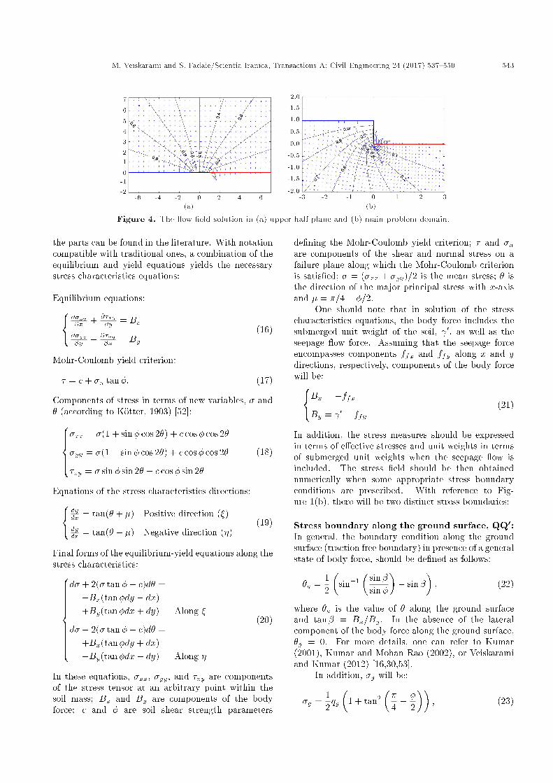
In these equations, i is the hydraulic gradient vector, w is the unit weight of the water, and ff (withcomponents ffu and ffv) is the vector of the unitseepage force, i.e. seepage force per unit volume. Theseepage force acts as �eld of body force with variablemagnitude and direction corresponding to the complexnature of the seepage ow pattern through the soil.Figure 4 presents the solution of the ow �eld for a unitvalue of Hw=Hs along with the associated hydraulicgradient vector �eld. In the next part, this vector�eld is incorporated into equations of the stress �eldto establish all necessary equations.

4. Solution of the stress �eld

So far, the solution of the ow force �eld has been pre-sented. Now, the stress �eld can be computed through-out the region within which failure would occur. This isdone by making use of the well-known method of stresscharacteristics. The technical literature behind thismethod and its development date back to Sokolovskii(1960, 1965) [11,46] and later works by a numberof authors who employed this method to deal withthe bearing capacity or retaining wall problems (Harr,1966; Houlsby and Wroth, 1982; Bolton and Lau,1993; Anvar and Ghahramani, 1997; Kumar, 2001;Kumar and Chitikela, 2002; Martin, 2003 and 2005;Veiskarami et al., 2014) [15-17,28,47-51]. We presentonly the necessary elements of this method as most of


Figure 4. The ow �eld solution in (a) upper half plane and (b) main problem domain.

the parts can be found in the literature. With notationcompatible with traditional ones, a combination of theequilibrium and yield equations yields the necessarystress characteristics equations:

Equilibrium equations:8<:@�xx@x + @�xy

@y = Bx@�yy@y + @�xy

@x = By(16)

Mohr-Coulomb yield criterion:

� = c+ �n tan�: (17)

Components of stress in terms of new variables, � and� (according to K�otter, 1903) [52]:8>>><>>>:

�xx = �(1 + sin� cos 2�) + c cos� cos 2�

�yy = �(1� sin� cos 2�) + c cos� cos 2�

�xy = � sin� sin 2� + c cos� sin 2�

(18)

Equations of the stress characteristics directions:8<: dydx = tan(� + �) Positive direction (�)dydx = tan(� � �) Negative direction (�)

(19)

Final forms of the equilibrium-yield equations along thestress characteristics:8>>>>>>>>><>>>>>>>>>:

d� + 2(� tan�+ c)d� =�Bx(tan�dy � dx)+By(tan�dx+ dy) Along �

d� � 2(� tan�+ c)d� =+Bx(tan�dy + dx)�By(tan�dx� dy) Along �

(20)

In these equations, �xx, �yy, and �xy are componentsof the stress tensor at an arbitrary point within thesoil mass; Bx and By are components of the bodyforce; c and � are soil shear strength parameters

de�ning the Mohr-Coulomb yield criterion; � and �nare components of the shear and normal stress on afailure plane along which the Mohr-Coulomb criterionis satis�ed; � = (�xx + �yy)=2 is the mean stress; � isthe direction of the major principal stress with x-axisand � = �=4� �=2.

One should note that in solution of the stresscharacteristics equations, the body force includes thesubmerged unit weight of the soil, 0, as well as theseepage ow force. Assuming that the seepage forceencompasses components ffx and ffy along x and ydirections, respectively, components of the body forcewill be:8<:Bx = �ffx

By = 0 � ffy(21)

In addition, the stress measures should be expressedin terms of e�ective stresses and unit weights in termsof submerged unit weights when the seepage ow isincluded. The stress �eld should be then obtainednumerically when some appropriate stress boundaryconditions are prescribed. With reference to Fig-ure 1(b), there will be two distinct stress boundaries:

Stress boundary along the ground surface, QQ0:In general, the boundary condition along the groundsurface (traction free boundary) in presence of a generalstate of body force, should be de�ned as follows:

�g =12

�sin�1

�sin�sin�

�� sin�

�; (22)

where �g is the value of � along the ground surfaceand tan� = Bx=By. In the absence of the lateralcomponent of the body force along the ground surface,�g = 0. For more details, one can refer to Kumar(2001), Kumar and Mohan Rao (2002), or Veiskaramiand Kumar (2012) [16,30,53].

In addition, �g will be:

�g =12qg�

1 + tan2��4

+�2

��; (23)


where qg is the surcharge pressure along the groundsurface. It is notable that it is convenient to de�ne avery small qg to prevent trivial solution in the stresscharacteristics equations. Referring to Bolton and Lau(1993) [48], it is often chosen, such that a dimensionlessratio = qg= 0B0 becomes a very small value, say, lessthan 0.01.

Stress boundary along the equivalent footingbase, BQ: Along this boundary, there is only thevalue of � = �f which should be de�ned. As statedearlier, it can be assumed that no signi�cant shearstress is mobilized at the equivalent footing interfacewith the top soil block, APQB, and hence, it is equalto zero.

5. Veri�cations

Now, the solution strategy obtained so far should beveri�ed. There is no available technique or similarresults on the analysis of deep-seated failure in presenceof the seepage ow, at least known to the authors.However, a simple and rational procedure was sug-gested by Terzaghi (1943) [3] for cases without seepage ow which is presented to make preliminary checks.Moreover, this procedure can be extended to the caseof the seepage ow by arti�cial techniques based onsimpli�ed assumptions. As an example problem, anarbitrary case of a supported vertical cut into a layerof uniform sand with and without seepage ow isanalyzed. Since all dimensions are normalized to theheight of the cut, Hs, thus, it is automatically equalto 1. Soil characteristic parameters are 0 = 10 kN/m3

and �0 = 25�. Analyses were made by using Eq. (1) forthe factor of safety.

Results of the analyses are presented in Table 1.In Case 1, the hydraulic head di�erence, Hw, betweenthe upstream and downstream water levels is zero. Inother cases, this di�erence grows to a critical value.In addition, when applying the method of Terzaghi

(1943) [3] to cases with seepage ow, it is conservativelyassumed that the hydraulic head is linearly dissipatedalong the wall length. Therefore, a very rough andconservative estimate of the hydraulic gradient hasbeen made. The hydraulic gradient obtained by thisway is reasonably higher than the average hydraulicgradient within the soil block which is simply id =Hw=Hs. This hydraulic gradient is then used toamplify the weight of the soil block to be supportedby the equivalent footing. Instead, no correction isaccounted for the seepage ow through the plasticregion beneath the equivalent footing and conventionalbearing capacity factor, N , implemented. In addition,Terzaghi (1943) [3], based on numerical results for caseswithout inclusion of the seepage ow, showed that thewidth of the equivalent footing, i.e., the B0=Hs ratio,falls within the range of 0.18 to 0.19. For those casesanalyzed by Terzaghi's method, this ratio is assumedto be 0.19.

In application of Eq. (1) when using Terzaghi(1943) method, the third bearing capacity factor, N ,was taken as 9.7 [3]. In addition, another try was madebased on the numerical results of N by Bolton andLau (1993) [48] by the method of stress characteristicswhich gave N = 3:51. The downward seepage owforce (to be added to the weight of the soil block), Ffd,was equal to 0:19 idH2

s . Also, the shear resistance, S,mobilized along the soil block was assumed to be:

S =12 0H2

sKA tan�0; (24)

where KA is the active earth pressure coe�cient. Thislatter assumption on S was also chosen as suggested byTerzaghi (1943) [3].

In the present approach, however, neither of theabovementioned assumptions is made. A more precisecalculation based on the present procedure can beperformed where the average of the hydraulic gradientthrough the soil block can be calculated. Moreover,the bearing capacity of the equivalent footing has been

Table 1. Results of the stability analysis for example problem.

MethodCase 1:

Hw=Hs = 0 (no ow)Case 2:

Hw=Hs = 0:25Case 3:

Hw=Hs = 0:50B0cr Fmin

s B0cr Fmins B0cr Fmin

s

Conventional approach(Terzaghi, 1943)

0.19 3.699 0.19 3.466 0.19 3.283

Conventional approach(Bolton and Lau, 1993)

0.19 1.329 0.19 1.254 0.19 1.188

Present study1 0.19 1.267 0.27 1.079 0.31 0.941

Present study2 0.19 1.267 0.26 1.243 0.29 1.0401 Variable seepage force; 2 Constant seepage force (averaged value).


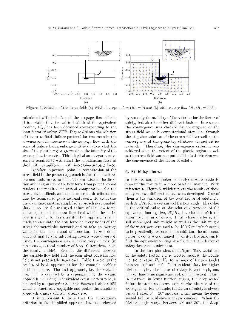
Figure 5. Solution of the stress �eld: (a) Without seepage ow (Hw = 0) and (b) with seepage ow (Hw=Hs = 0:25).

calculated with inclusion of the seepage ow e�ects.It is notable that the critical width of the equivalentfooting, B0cr, has been obtained corresponding to theleast factor of safety, Fmin

s . Figure 5 shows the solutionof the stress �eld (failure pattern) for two cases in theabsence and in presence of the seepage ow with thezone of failure being enlarged. It is obvious that thesize of the plastic region grows when the intensity of theseepage ow increases. This is logical as a larger passivezone is required to withstand the unbalancing force atthe limiting equilibrium with increasing seepage force.

Another important point in computation of thestress �eld in the present approach is that the ow forceis a non-uniform vector �eld. The variation in the direc-tion and magnitude of the ow force from point to pointrenders the required numerical computations for thestress �eld di�cult and much more mesh re�nementsmay be required to get a rational result. To avoid thisdisadvantage, another simpli�ed approach is suggested,that is, to use the averaged values of the ow force,as an equivalent constant ow �eld within the entireplastic region. To do so, an iteration approach can bemade to calculate the ow force at every nodes of thestress characteristics network and to take an averagevalue for the next round of iteration. It was done,and fortunately two interesting results were observed.First, the convergence was achieved very quickly (inmost cases, a total number of 5 to 10 iterations makethe results stable). Second, the di�erence betweenthe variable ow �eld and the equivalent constant ow�eld is not practically signi�cant. Table 1 presents theresults of both approaches for the example problemoutlined before. The �rst approach, i.e. the variable ow �eld is denoted by a superscript 1; the secondapproach, i.e. using an equivalent constant ow �eld, isdenoted by a superscript 2. The di�erence is about 10%which is practically negligible and makes the simpli�edapproach a more e�cient alternative.

It is important to note that the convergencecriterion in the simpli�ed approach has been checked

by not only the stability of the solution for the factor ofsafety, but also for other di�erent factors. In essence,the convergence was checked by convergence of thestress �eld at each computational step, i.e. throughthe stepwise solution of the stress �eld as well as theconvergence of the geometry of stress characteristicsnetwork. Therefore, the convergence criterion wasachieved when the extent of the plastic region as wellas the stress �eld was computed. The last criterion wasthe convergence of the factor of safety.

6. Stability charts

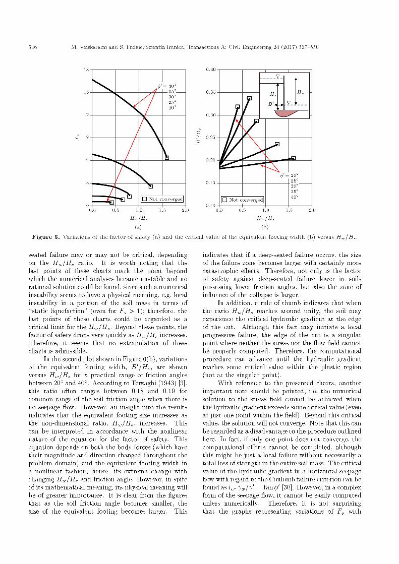
In this section, a number of analyses were made topresent the results in a more practical manner. Withreference to Figure 6, which re ects the results of theseanalyses, two di�erent charts were developed. One ofthem is the variation of the least factor of safety, Fs,with Hw=Hs for a certain soil friction angle. The otheris the critical value of the relative dimension of theequivalent footing size, B0=Hs, i.e. the one with thelowermost factor of safety. In all these analyses, thesoil submerged unit weight as well as the unit weightof the water were assumed to be 10 kN/m3 which seemsto be practically reasonable. In addition, the minimumfactor of safety was obtained by an iterative analysis to�nd the equivalent footing size for which the factor ofsafety becomes a minimum.

In the �rst plot shown in Figure 6(a), variationsof the safety factor, Fs, is plotted against the nondi-mensional ratio, Hw=Hs, for a range of friction anglesbetween 20� and 40�. It is evident that for higherfriction angles, the factor of safety is very high, andhence, there is no signi�cant risk of deep seated failure.In contrast, in lower friction angles, the deep-seatedfailure is prone to occur, even in the absence of theseepage ow. For example, the factor of safety is alwaysbelow 1 when �0 = 20� and less, which means the deep-seated failure is always a major concern. When thefriction angle ranges between 20� and 30�, the deep-


Figure 6. Variations of the factor of safety (a) and the critical value of the equivalent footing width (b) versus Hw=Hs.

seated failure may or may not be critical, dependingon the Hw=Hs ratio. It is worth noting that thelast points of these charts mark the point beyondwhich the numerical analyses became unstable and norational solution could be found, since such a numericalinstability seems to have a physical meaning, e.g. localinstability in a portion of the soil mass in terms of\static liquefaction" (even for Fs > 1); therefore, thelast points of these charts could be regarded as acritical limit for the Hw=Hs. Beyond these points, thefactor of safety drops very quickly as Hw=Hs increases.Therefore, it seems that no extrapolation of thesecharts is admissible.

In the second plot shown in Figure 6(b), variationsof the equivalent footing width, B0=Hs, are shownversus Hw=Hs for a practical range of friction anglesbetween 20� and 40�. According to Terzaghi (1943) [3],this ratio often ranges between 0.18 and 0.19 forcommon range of the soil friction angle when there isno seepage ow. However, an insight into the resultsindicates that the equivalent footing size increases asthe non-dimensional ratio, Hw=Hs, increases. Thiscan be interpreted in accordance with the nonlinearnature of the equation for the factor of safety. Thisequation depends on both the body forces (which havetheir magnitude and direction changed throughout theproblem domain) and the equivalent footing width ina nonlinear fashion; hence, its extrema change withchanging Hw=Hs and friction angle. However, in spiteof its mathematical meaning, its physical meaning willbe of greater importance. It is clear from the �guresthat as the soil friction angle becomes smaller, thesize of the equivalent footing becomes larger. This

indicates that if a deep-seated failure occurs, the sizeof the failure zone becomes larger with certainly morecatastrophic e�ects. Therefore, not only is the factorof safety against deep-seated failure lower in soilspossessing lower friction angles, but also the zone ofin uence of the collapse is larger.

In addition, a rule of thumb indicates that whenthe ratio Hw=Hs reaches around unity, the soil mayexperience the critical hydraulic gradient at the edgeof the cut. Although this fact may initiate a localprogressive failure, the edge of the cut is a singularpoint where neither the stress nor the ow �eld cannotbe properly computed. Therefore, the computationalprocedure can advance until the hydraulic gradientreaches some critical value within the plastic region(not at the singular point).

With reference to the presented charts, anotherimportant note should be pointed, i.e. the numericalsolution to the stress �eld cannot be achieved whenthe hydraulic gradient exceeds some critical value (evenat just one point within the �eld). Beyond this criticalvalue, the solution will not converge. Note that this canbe regarded as a disadvantage to the procedure outlinedhere. In fact, if only one point does not converge, thecomputational e�orts cannot be completed, althoughthis might be just a local failure without necessarily atotal loss of strength in the entire soil mass. The criticalvalue of the hydraulic gradient in a horizontal seepage ow with regard to the Coulomb failure criterion can befound as icr w= 0 = tan�0 [30]. However, in a complexform of the seepage ow, it cannot be easily computedunless numerically. Therefore, it is not surprisingthat the graphs representing variations of Fs with


Figure 7. Variations of the equivalent footing width,B0=Hs with �0.

Hw=Hs are terminated at some point di�erent fromFs = 0. These points are denoted by a small square(i.e., was not converged) in the presented graphs. Inaddition, these points have a physical meaning, i.e.when the soil becomes unstable at some point withinthe plastic region, this instability becomes the onset ofa progressive failure starting just from that particularpoint. Furthermore, as soon as this instability isreached, the initiation of a failure should be expected inspite of the overall factor of safety (which may be stillhigher than unity). Thus, it is not su�cient to have afactor of safety higher than unity, but it is necessaryto avoid approaching such critical points following aprogressive failure.

Finally, variations of the equivalent footing width,B0=Hs, with the soil friction angle are plotted inFigure 7. One should note that a small part of thesegraphs has been produced back by extrapolation of theresults (for �0 = 20� and 25� only). Such curves couldnot be produced with su�cient accuracy for frictionangle �0 below 20� due to convergence error. Theseplots are useful for a simpli�ed approach based on anaverage of the hydraulic gradient.

7. Conclusions

A semi-analytical study was performed to includethe e�ect of the seepage ow on the stability of asupported vertical cut against deep-seated (or base)failure in waterfront excavations. This is a problem forwhich no analytical solution is available and numericaltechniques involve complications. In the presentedsemi-analytic procedure, the e�ect of the seepage owhas been included by solution of the ow �eld asan independent and analytical solution (backgroundsolution) and the solution of the stress �eld at thelimiting equilibrium as the main solution (by numericaltechniques). In this procedure, it is formally assumedthat the ow �eld pattern is not in uenced by the

formation of a failure mechanism. Such an assumptiondoes not seem to be too much restrictive; hence, thesolution of the ow �eld can be found independently.The solution of the ow �eld was found by succes-sive applications of conformal mappings in complexplanes and the simple solution of the steady-state owproblem in a semi-in�nite strip in the complex plane.The presented approach has several advantages overother fully numerical methods, e.g. higher accuracy andspeed.

Analyses showed that the deep-seated failure is of-ten a critical criterion to design supported excavations,which deserves more attention. In fact, for practicalrange of friction angle for most sands, the probabilityof failure increases signi�cantly when the cut is exposedto the seepage ow. In cases with low friction angle, like�ne sands, such a failure may dominate the design andmay precede other types of failure such as the slopefailure (often not a major concern), wall failure (dueto insu�cient passive pressure and increased activepressure) or piping, and heaving failures. In addition,results revealed that the size of the collapse patterngrows signi�cantly as the soil friction angle decreases.Thus, it can be concluded that not only the probabilityof failure can increase for such soils, but also the type offailure can be more catastrophic which requires furtherserious provisions in practice.

References

1. Coulomb, C. A., Essay on an Application of the Rulesof Maximal and Minimal to Some Problems of StaticsRelating to Architecture, [Essai sur une Application desR�egles des Maximisn et Minimis �a QuelquesProbl�emesde Statique Relatifs �a L'Architecture], 7. Paris, France:Mem. Acad. Roy. Pres. Div. Sav. (1776).

2. Rankine, W.J.M., On the Stability of Loose Earth.London, UK: Phil. Trans. Royal Soc. (1857).

3. Terzaghi, K., Theoretical Soil Mechanics, NY: John-Wiley and Sons Inc.(1943).

4. Kumar, J. and Subba Rao, K.S. \Passive pressurecoe�cients, critical failure surface and its kinematicadmissibility", G�otechnique, 47(1), pp. 185-192 (1997).

5. Subba Rao, K.S. and Choudhury, D. \Seismic passiveearth pressures in soils", Journal of Geotechnical andGeoenvironmental Engineering, ASCE, 131(1), pp.131-135 (2005).

6. Barros, P.L.A. \A coulomb-type solution for activeearth thrust with seepage", G�ootechnique, 56(3), pp.159-164 (2006).

7. Ghosh, P. \Seismic active earth pressure behind a non-vertical retaining wall using pseudo-dynamic analysis",Can. Geotech. J., 45(1), pp. 117-123 (2008).

8. Ghosh, S. and Sharma, R.P. \Pseudo-dynamic evalua-tion of passive response on the back of a retaining wall


supporting c-' back�ll", Geomechanics and Geoengi-neering: An International Journal, Taylor and Francis,7(2), pp. 115-121 (2012).

9. Barros, P.L.A. and Santos, P.J. \Coe�cients of activeearth pressure with seepage e�ect", Can. Geotech J.,49(6), pp. 651-658 (2012).

10. Ling, H., Ling, H.I. and Kawataba, T. \Revis-iting nigawa landslide of the 1995 Kobe earth-quake", G�ootechnique, 64(5), pp. 400-404 (2014). DOI:10.1680/geot.12.T.019

11. Sokolovskii, V.V., Statics of Granular Media, London:Pergamon (1965).

12. Larkin, L.A. \Theoretical bearing capacity of veryshallow footings", Journal of the Soil Mechanics andFoundations Division ASCE, 94(6), pp. 1347-1357(1968).

13. Sabzevari, A. and Ghahramani, A. \The limit equi-librium analysis of bearing capacity and earth pres-sure problems in nonhomogeneous soils", Soils andFoundations, Japanese Society of Soil Mechanics andFoundations Engineering, 12(3), pp. 33-48 (1972).

14. Sabzevari, A. and Ghahramani, A. \Theoretical inves-tigation on the passive progressive failure in an earthpressure problem", Soils and Foundations, JapaneseSociety of Soil Mechanics and Foundations Engineer-ing, 13(2), pp. 1-18 (1973) .

15. Houlsby, G.T. and Wroth, C.P. \Direct solution ofplasticity problems in soils by the method of charac-teristics", Proc. 4th Intl. Conf. Num. Meth. Geomech.,Edmonton, 3, pp. 1059-1071 (1982).

16. Kumar, J. \Seismic passive earth pressure coe�cientsfor sands", Can. Geotech. J., 38(4), pp. 876-881(2001).

17. Kumar, J. and Chitikela, S. \Seismic passive earthpressure coe�cients using the method of characteris-tics", Can. Geotech. J., 39(2), pp. 463-471 (2002).

18. Chen, W.-F. \Soil mechanics and theorems of limitanalysis", Journal of the Soil Mechanics and Founda-tions Division, ASCE, 95(SM2), pp. 493-518 (1969).

19. Lysmer, J. \Limit analysis of plane problems insoil mechanics", Journal of the Soil Mechanics andFoundations Division, ASCE, 96(SM4), pp. 1311-1334(1970).

20. Chen, W-F. and Davidson, H.L. \Bearing capacity de-termination by limit analysis", Journal of the Soil Me-chanics and Foundations Division, ASCE, 99(SM6),pp. 433-449 (1973).

21. Collins, I.F. \A note on the interpretation of coulomb'sanalysis of the thrust on a rough retaining Wall interms of the limit theorems of plasticity theory",G�ootechnique, 23(3), pp. 442-447(1973).

22. Chen, W-F., Limit Analysis and Soil Plasticity, Else-vier (1975).

23. Arai, K. and Jinki, R. \A lower-bound approach toactive and passive earth pressure problems", Soils and

Foundations. Japanese Society of Soil Mechanics andFoundations Engineering, 30(4), pp. 25-41 (1990) .

24. Soubra, A.-H. \Static and seismic passive earth pres-sure coe�cients on rigid retaining structures", Can.Geotech. J., 37(1), pp. 463-478 (2000).

25. Soubra, A-H. and Macuh, B. \Active and passiveearth pressure coe�cients by a kinematical approach",Geotechnical Engineering, 155(2), pp. 119-131 (2002).

26. Shiau, J.S., Augarde, C.E., Lyamin, A.V. and Sloan,S.W. \Finite element limit analysis of passive earth re-sistance in coehesionless soils", Soils and Foundations,48(6), pp. 843-850 (2008).

27. Jahanandish, M., Veiskarami, M. and Ghahramani,A. \E�ect of stress Level on the bearing capacityfactor, N , by ZEL Method", KSCE Journal of CivilEngineering, Springer, 14(5), pp. 709-723 (2010).

28. Veiskarami, M., Kumar, J. and Valikhah, F. \E�ectof the ow rule on the bearing capacity of stripfoundations on sand by the upper-bound Limit anal-ysis and slip lines", International Journal of Ge-omechanics, ASCE, 14(3), 04014008 (2014). DOI:10.1061/(ASCE)GM.1943-5622.0000324

29. Kawamura, M. and Watanabe, T. \Stress analysisof earth pressure with seepage ow during heavyrainstorms", Proc. 9th Southeast Asian GeotechnicalConference, Publication in Bangkok: Southeast AsianGeotechnical Society. Bangkok, 7-11 Dec. 1987 (1)2.53-2.62, (1989). DOI: 10.1016/0148-9062(89)92828-3

30. Kumar, J. and Chakraborty, D. \Bearing capacityof foundations with inclined ground water seepage",International Journal of Geomechanics, ASCE, 13(5),pp. 611-624 (2013).

31. Veiskarami, M. and Kumar, J. \Bearing capacity offoundations subjected to groundwater ow", Geome-chanics and Geoengineering: An International Jour-nal, Taylor and Francis, 7(4), pp. 293-301 (2012).

32. Soubra, A.-H., Kastner, R. and Benmansour, A.\Passive earth pressures in the presence of hydraulicgradients", G�ootechnique, 49(3), pp. 319-331 (1999).

33. Benmebarek, N., Benmebarek, S., Kastner, R. andSoubra, A.-H. \Passive and active earth pressuresin the presence of groundwater ow", G�ootechnique,56(3), pp. 149-158 (2006).

34. Santos, P.J. and Barros, P.L.A. \Active earth pres-sure due to a soil mass partially subjected to waterseepage", Can. Geotech. J., (In Press) (2015). DOI:10.1139/cgj-2014-0367)

35. Veiskarami, M. and Zanj, A. \Stability of sheet-pilewalls subjected to seepage ow by slip lines and �niteelements", G�ootechnique, 64(10), pp. 759-775 (2014).

36. Craig, R.F., Soil Mechanics, 4th Ed., Chapman andHall, London, UK (1987).

37. Bowles, J.E., Foundation Analysis and Design, 5thEd.,McGraw Hill, New York, USA (1996).


38. Veiskarami, M. and Habibagahi, G. \Foundationsbearing capacity subjected to seepage by the kinematicapproach of the limit analysis", Frontiers of Structuraland Civil Engineering, 7(4), pp. 446-455 (2013).

39. Harr, M.E., Groundwater and Seepage, McGraw-Hill,New York (1962).

40. Christian, J.T. \Flow nets from �nite-element data",Int. J. Numer. Anal. Meth. Geomech., John-Wiley andSons, 4(2), pp. 191-196 (1980).

41. Gri�ths, D.V. \Seepage beneath unsymmetric co�er-dams", G�ootechnique, 44(2), pp. 297-305 (1994).

42. Zienkiewicz, O.C. and Taylor, R.L., The Finite Ele-ment Method, 5th Ed. Butterworth-Heinemann, UK(2000).

43. Kiousis, P.D. \Least-squares �nite-element evaluationof ow nets", Journal of Geotechnical and Geoenvi-ronmental Engineering, ASCE, 128(8), pp. 699-701(2002).

44. Churchill, R.V., Brown, J.W. and Verhey, R.F., Com-plex Variables and Applications, 3rd Ed., McGraw Hill,New York, USA (1974).

45. Mathews, J.H. and Howell, R.W., Complex Analysisfor Mathematics and Engineering, 3rd Ed., Jones andBartlett, Sudbury, Massachusetts, USA (1997).

46. Sokolovskii, V.V., Statics of Soil Media (translatedby D.H. Jones and A.N. Scho�eld)., Butterworths,London, UK (1960).

47. Harr, M.E., Foundations of Theoretical Soil Mechan-ics, McGraw-Hill, NY, USA (1966).

48. Bolton, M.D. and Lau, C.K. \Vertical bearing capac-ity factors for circular and strip footings on Mohr-Coulomb soil", Can. Geotech. J., 30(6), pp. 1024-1033(1993). DOI: 10.1139/t93-099.

49. Anvar, S.A. and Ghahramani, A. \Equilibrium equa-tions on zero extension lines and their application tosoil engineering", Iranian Journal of Science and Tech-nology (IJST), Shiraz University Press, Transaction B,21(1), pp. 11-34 (1997).

50. Martin, C. M. \ABC - analysis of bearing capacity(user guide for)" OUEL Report No. 2261/03, Uni-versity of Oxford, UK, (2003). URL: http://www.eng.ox.ac.uk/civil/people/cmm/software

51. Martin, C.M. \Exact bearing capacity calculationsusing the method of characteristics", Proc. 11th Int.Conf. ofIACMAG, 4, Turin, France, pp. 441-450(2005).

52. K�otter, F., Determination of Pressure on Curved Slid-ing Surfaces, a Task from the Theory of Earth Pres-sure [Die Bestimmung des Druckes an gekr�ummtenGleit �achen, eine Aufgabe aus der Lehre vom Erd-druck], Sitzungsberichte der Akademie der Wis-senschaften, pp. 229-233, Berlin, Germany (1903).

53. Kumar, J. and Mohan-Rao. \Seismic bearing capacityfactors for spread foundations", G�ootechnique, 52(2),pp. 79-88 (2002).

Appendix A

Successive transformations from w3-plane toz-planeThe problem domain and the solution can be trans-formed from w3-plane to z-plane by the followingsuccessive conformal mappings. With reference toFigure 3:

w3 = sin�1 w2 or inversely: w= sinw3: (A.1a)

Moreover:

w2 =u2 + iv2 = sin(u3 + iv3) = sinu3 cosh v3

+ i cosu3 sinh v3: (A.1b)

Therefore:

u2 = sinu3 cosh v3 and v2 = cosu3 sinh v3: (A.1c)

However, according to trigonometric relationships:�u2

sinu3

�2

��

v2

cosu3

�2

= 1: (A.1d)

Thus:

u3 =sin�1�q

(u2+1)2+v22�q

(u2�1)2+v22

�;(A.1e)

which is required for the rest of calculations.Transformation between w1-plane and w2-plane is

obtained by:

w2 = w1=21 or inversely w1 = w2

2: (A.2a)

Consequently:

u1 + iv1 = (u2 + iv2)2: (A.2b)

which yields:(u2 = � 1p

2

qu1 �pu2

1 + v21

v2 = v12u2

= v12u2

(A.2c)

Transformation between z-plane and w1-plane is ob-tained by:

w1 =z + 1

2or inversely: z = 2w1 � 1: (A.3a)

Therefore:

u1 =x+ 1

2and v1 =

y2: (A.3b)

These transformations can be directly used to transferboth the geometry and the solution of the problem;hence, the solution will be available in complex z-plane.


Appendix B

Solution of the hydraulic gradient in complexw-planeThe gradient of the hydraulic head required to computethe seepage ow force can be found as follows.

First of all, one should obtain the Jacobianof the transformation which requires some arti�cialmanipulations by the aid of functions Re(w(z)) andIm(w(z)) which bring the real and imaginary parts ofa complex function and can be easily programmed inMATLAB or other similar environments:

[J ] =�@u@x

@v@x

@u@y

@v@y

�; (B.1)

@u@x

=�1�

Re�

2x+2iy2p

(x+iy)2�1+

1p(x+iy)2�1

�; (B.2)

@u@y

=�1�

Re�

2ix�2y2p

(x+iy)2�1+

ip(x+iy)2�1

�; (B.3)

@v@x

=�1�

Im�

2x+2iy2p

(x+iy)2�1+

1p(x+iy)2�1

�; (B.4)

@v@y

=�1�

Im�

2ix�2y2p

(x+iy)2�1+

ip(x+iy)2�1

�: (B.5)

Having known the coordinates of an arbitrary point, inthe main problem domain, the inverse of the Jacobianmatrix can be found for the rest of calculations.In addition, the components of the gradient of thehydraulic head, rh, can be calculated by Eqs. (B.6)to (B.8) as shown in Box I.

It is notable that the inverse problem, i.e. map-ping from the w-plane onto the z-plane, may be alittle complicated and long; however, the location of

every arbitrary point in the w-plane can be found by anumerical technique like the Newton-Raphson methodas the entire problem, i.e. solution of the ow �eld andlater, solution of the stress �eld, should be traditionallyrecast in a computer code.

Biographies

Mehdi Veiskarami has received his BSc and MScdegrees from the University of Guilan and receivedhis PhD degree from Shiraz University in 2010 undersupervision of Prof. Arsalan Ghahramani and Prof.Mojtaba Jahanandish. His PhD dissertation was onthe load-displacement behavior and bearing capacityof shallow foundations by the ZEL method, consideringthe stress level e�ect. He has published several papersin the �eld of geomechanics and coauthored a bookon mat foundations analysis and design which waspublished by the University of Guilan press in 2006.Dr. Mehdi Veiskarami is currently serving as a facultymember and visiting scholar at Shiraz University whilehe is simultaneously an Assistant Professor in theUniversity of Guilan.

Sina Fadaie has received both BSc and MSc degreesfrom the University of Guilan. During his masterprogram, he was awarded the outstanding graduatestudent and his thesis was recognized as one of theselected theses in the area of Geotechnical Engineeringin Guilan Province by a research council determinedby the municipality of Rasht. His master thesis was onthe stability of supported vertical cuts against deep-seated failure when they are prone to the seepage owby a hybrid numerical method. He worked undersupervision of Dr. Mehdi Veiskarami in the Universityof Guilan and graduated in early 2016. He has recentlypublished several papers from his research results.

rh =@h@x

ex +@h@y

ey; (B.6)

@h@x

= � 1�

0B@ � x�12p

(x�1)2+y2+ x+1

2p

(x+1)2+y2�p(x+ 1)2 + y2

�=�

1� 12

p(x� 1)2 + y2 � 1

2

p(x+ 1)2 + y2

�2

1CA12

; (B.7)

@h@y

= � 1�

0B@ � y2p

(x�1)2+y2+ x+1

2p

(x+1)2+y2�1� 1

2

p(x� 1)2 + y2 � 1

2

p(x+ 1)2 + y2

�2

1CA12

: (B.8)

Box I

Documents

Stability of supported vertical cuts in granular matters ...scientiairanica.sharif.edu/article_2416_58043afd9c4ccfaf6119f3a... · Stability of supported vertical cuts in granular