Embed Size (px)
Citation preview

LOCAL STABILITY OF STATIONARY EQUILIBRIA(VERY PRELIMINARY AND VERY INCOMPLETE)
MARCIN PĘSKI AND BALAZS SZENTES
Abstract. This paper characterizes stable stationary equilibria in large popula-tion dynamic games. Each player has a type which changes over time. A player’sflow payoff as well as the evolution of her type depends on the distribution of popu-lation types and population strategies. A stationary equilibrium is called stable if,after perturbing the equilibrium strategies slightly, revision dynamics converge backto the equilibrium. We derive simple sufficient (and almost necesarry) conditionsfor stability. These conditions involve eigenvalues of a one-dimensional familiy ofmatrices. Moreover, in order to check whether an equilibrium is stable, it is enoughto consider sine wave perturbations of the equilibrium.
1. Introduction
A large literature on learning is concerned with the convergence of boundedly ratio-nal best-response dynamics. Players receive opportunities to revise their actions andsome information about the actions of others. Players ignore the fact that others willupdate their actions in the future, and best-responde to the current action profile asif it was never to change. This literature typically focuses on learning in normal formgames. That is, the game played in each period is the same. In this paper, we seek todevelop a theory of learning in dynamic games, where the game that agents face ineach period is potentially different and its can depend on the population strategies.
In the specific model analysed in this paper, there is a continuum of agents. Eachagent has a finite type space. The type of an agent changes over (continuous) time,and its evolution as well as the agent’s payoffs are determined by the strategy ofthe agent, the strategies and types of the others. Because current actions affect notonly current payoffs but also future distribution of types and payoffs, the agents have
Date: 05/30/13.1

2 MARCIN PĘSKI AND BALAZS SZENTES
long-run incentives.1 An equilibrium is called stationary if neither the populationstrategies, nor the distribution of types change over time. We seek to characterizethe stable stationary equilibria of our model. An equilibrium is called stable if, afterperturbing the equilibrium strategies slightly, revision dynamics imply convergenceback to the equilibrium. In order to model revision dynamics, we assume that eachplayer stochastically receives rare opportunities to update her strategy. Whenever aplayer has this opportunity, she forms a prediction regarding the population strategiesand adjusts her strategy to best respond to the predicted environment.
Let us explain the main conceptual difficulty of extending the theory of learningto dynamic games. The standard assumption in the context of static games is thatwhenever an agent revises her behavior, she acts under a myopic assumption that theother players actions are never going to be updated in the future.2 If the game isdynamic, an agent’s strategy is a mapping from the set of future periods to actions.Even if the agent ignores the others’ opportunities to revise their strategies, she stillconsider a possibility that the actions played will vary in time. Therefore, one mustcarefully model how the prediction about population strategies are formed.
We consider two scenarios regarding how players form their predictions. In thefirst scenario, whenever a player can revise her strategy she perfectly observes thestrategies of the others. In other words, a player understands perfectly well how theaction of others vary in time. The dynamic generated from these predictions is thestraightforward conceptual generalization of the myopic best-response dynamics innormal form games and we refer to as best-response dynamic. Assuming that agentsobserve population log-run strategies is obviously problematic because at the moment,these strategies exist as intentions, yet to be executed. We treat the best-responsedynamic as a benchmark. In the second scenario, players observe past actions of theothers and forecast their strategies from detected patterns. Players can only detectpatterns with certain fixed frequencies, including the zero frequency that correspondsto constant average actions. By varying the detectable frequencies, we can consider
1Our model is a continuous time version of dynamic games widely used across the economic theory(examples include ?, ?, ?, and ?).
2For the overview of the theory of learning in static games see see ?, ?, or ?.

STABILITY OF STATIONARY EQULIBRIA 3
different levels of sophistication. For example, if only actions can be observed, thedynamic extends standard model of fictitious play. We refer to such a dynamic aslearning dynamic.
The main result of this paper is a characterization of stable stationary equilibriaof our model when the revision opportunities are rare. We first show that in order tocheck whether an equilibrium is stable, it is enough to consider sine wave perturba-tions of the equilibrium. A sine wave perturbation is essentially a repetitive oscillationaround the equilibrium strategy. A particular perturbation can be parametrized bythe frequency of the oscillation and the “amplitude” vector of actions. It turns outthat the best response to such a sine wave perturbation of a certain frequency iswell-approximated by another sine wave perturbation of the same frequency. More-over, the relationship between the perturbation and the (approximate) best responseis linear, and hence, the best-response operator can be identified with a matrix. Ofcourse, this matrix depends on the frequency of the oscillation, and hence we needto consider a family of matrices parametrized by all possible frequencies. In the caseof best-response dynamics, our main result is that a stationary equilibrium is stableif the real part of all the eigenvalues of each matrix in this family is negative. Con-versely, if the real part of an eigenvalue of at least one matrix is strictly positive, theequilibrium is unstable. In the case of learning-dynamics, the real parts of the eigen-values need to be negative only of those matrices which correspond to a frequencywhich is detectable by the players.
Our results are limited to the case when the revision opportunities are rare. Moreprecisely, the sufficient conditions for stability may fail if the revision opportunitiesarrive fast (the necessary conditions remain necessary regardless of the speed of thedynamics). We view slow revision dynamics as more consistent with the spirit oflearning and bounded rationality that motivates the literature.
It is instructive to compare our results with analogous results known in the staticcase. The best response dynamic in the dynamic games is closely related to the con-tinuous time best response dynamic in static games; similarly, the learning dynamic isrelated to the models of fictitious play The asymptotic stability of a Nash equilibriumdepends on the eigenvalues of the Jacobian of the best response function computed

4 MARCIN PĘSKI AND BALAZS SZENTES
at the equilibrium. The main difference here is that the strategies in the dynamicmodels are much more complicated than in the static case. Instead of one, we need anentire one-dimensional family of matrices to characterize the stability. The role of thefrequency parameter ω is inherently dynamic as it describes how the strategies changeover time. It is worth to point out that the oscillations of strategies represent a differ-ent issue than the cycling of the dynamic. The latter appear if the eigenvalues haveimaginary components both in the static (matching pennies, or Rock-Scissors-Papergame) and in the dynamic case (see Section 3) below.
The paper is divided as follows. Section 2 introduces the model and the definitionsof the dynamics. Section 4 defines the constants that characterize the stability of anequilibrium. Section 3 discusses an example of a dynamic game with a unique sta-tionary equilibrium that is not stable with respect to the revision dynamics. Sections5, 6, and 7 characterize the stability of, respectively, the evolution type distributionwith respect to the perturbations of the type distribution, and the stability of thestationary equilibria with respect to the two kinds of revision dynamics. Section 8concludes. The Appendix contains all the proofs.
2. Model
Fix Banach space X. The norm on X is denoted with ‖.‖X or simply ‖.‖ wheneverit does not lead to confusion. Let X to denote the Banach space of all continuousfunctions χ : R+ → X with the “sup” norm, ‖χ‖X = supt≥0 ‖χt‖X . For each mea-sure space (C, C, µ), let D ((C, C, µ) ;X) denote the Banach space of (a.e. equivalenceclasses of) Bochner C-measurable, square-integrable with respect to Lebesgue mea-sure, mappings w : Ω → X with the L2-norm.3We also write D (C;X) or D (X) ifthe measurable structure or the entire measure space is known from the context. Weassume that X is immersed in X, and DX via constant mappings.
2.1. Dynamic game. Continuous time is indexed with t ∈ R. The players discountfuture payoffs at constant rate r > 0.
3Bochner spaces Lp (T ;X) for 1 ≤ p ≤ ∞ are generalization of standard Lp spaces of (equivalenceclasses of) measurable real-valued functions f : T → R to functions that take value in Banach spaceX. A function is Bochner measurable if it is an a.e. limit of countably-valued measurable functions.
STABILITY OF STATIONARY EQULIBRIA 5
There is a continuum of agents. In each period, each agent plays action a ∈ A,where the set of actions A is a finitely dimensional (Euclidean) space. Additionally,each agent has a private type θ that belongs to a finite set Θ. The types of the playersmay evolve throughout the game.
In each period, the agents payoffs and the dynamics of types depends on the currentaverage distribution e ∈ ∆ (A×Θ) over the actions and types in the population. Theinstantaneous payoffs of a player with action a and type θ are equal to∑
b,φ
e (b, φ) g (a, θ, b, φ) .
The type of a player evolves according to a Poisson process and its evolution isindependent from the evolution of the types of the other players. The rate at whichtype θ of a player changes into type θ′ 6= θ is equal to∑
b,φ
e (b, φ) γ (θ′; a, θ, b, φ) ≥ 0.
It is convenient to define the rate of “out” transitions out of state θ as
γ (θ; a, θ, b, φ) := −∑θ′ 6=θ
γ (θ′; a, θ, b, φ)
for all actions a, b ∈ A and types θ, φ. Define a vector of transition rates
γ (a, θ, b, φ) = [γ (θ′; a, θ, b, φ)]θ′∈Θ . (2.1)
Throughout the paper, we assume that functions g and γ are uniformly bounded, andtwice continuously differentiable in (a, b) with uniformly bounded derivatives. 4
Our model allows for the possibility that some types or their groups keep theirpopulation share fixed throughout the game, whereas the shares of other types (or
4The dependence of the payoffs and transition rates on the average distribution in the populationcan be interpreted as an outcome of random matching. The model is not restricted to uniformrandom matching as some other types of matching probabilities can be captured by appropriateadjustments in functions g and γ. For example, if types θ match with each other twice more oftenthan with other types, this can be modeled by multiplying function g (., θ, ., θ)by factor 2.
Additionally, the model and the result can be generalized to non-linear dependence of the payoffsand transitions on the average distribution e. We avoid the generalization in this version of thepaper to eliminate additional notation and definitions.

6 MARCIN PĘSKI AND BALAZS SZENTES
shares within the group) evolve depending on the strategies of the players. In theexample from Section 3, there are two classes of players 1 and 2 with the populationshare fixed at 1
2 . Within each class, there are subtypes θ = −1, 1 with evolving shares.This leads to four-element set of types Θ = (1,−1) , (1, 1) , (2,−1) , (2, 1).
It will be useful to explicitly model the restrictions on the attainable type dis-tributions. Let ΛΘ ⊆ ∆Θ be the subset of attainable probability distributions.Let Φ (Θ) ⊆ RΘ be the linear subspace spanned by the vector transition ratesγ (a, θ, b, φ) ∈ RΘ for all actions a, b and types θ, φ. Then, for each v, v′ ∈ ΛΘ,v − v′ ∈ Φ (Θ), and Φ (Θ) is the set of all possible directions of the evolution of thetype distribution. In the first reading, the reader may assume that ΛΘ consists ofall probability distributions and Φ (Θ) is equal to the set of all vectors υ ∈ RΘ withcoordinates that add up to 0.
2.2. Strategies. An agent plans her behavior by choosing a long-run strategy. Be-cause the influence of each individual on the rest of the population is negligent, weassume that a strategy depend only on time and the agent’s own type.5 Let A = AΘ
be the space of generalized actions, i.e., mappings α : Θ → A that assign properactions to states. A strategy is a continuous mapping σ : R+ → A with the inter-pretation that σt (θ) is an action taken by the agent if her private type is θ. Foreach strategy σ, each t > 0, let σ(t) be the t-period continuation strategy definedσ(t)s = σs+t. The space of strategies is denoted with A.A heterogeneous population is divided into cohorts c ∈ C. We assume that (C, C, µ)
is a non-atomic measure space of cohorts. A strategy profile is a measurable mappingw ∈ D
(A)with the interpretation that wct is the t-period (generalized) action played
by the members of cohort c. For each t > 0, let w(t) be the continuation strategy
5Alternatively, the strategies may depend not only on time, but also on the actions and the typesof the other agents. However, if we restrict the attention to the pure strategies, then all the bestresponses can be implemented with strategies that depend only on time (even if the strategies ofthe other agents are more complicated). That’s not necessarily true when the agents use mixedstrategies, but it will be true even with mixed strategies if we assume that the strategies do notdepend on the actions or types of any countable set of agents.

STABILITY OF STATIONARY EQULIBRIA 7
profile after t. For each strategy profile w, let wE ∈ A be the average strategy definedas wEt =
´wctdµ (c) .
Let v0 ∈ D (ΛΘ) be the profile of type distribution among the members of thecohorts in period 0. A strategy profile w and the profile of type distributions v0
determine the evolution of the type distributions v (w, v0) ∈ D(ΛΘ
)as a solution to
the following equation: v0 (w, v0) = v0, and for each t, each θ′,d
dtvct (θ′;w, v0) (2.2)
=ˆ
C
∑φ
∑θ 6=θ′
γ (θ′;wct (θ) , θ, wst (φ) , φ) vct (θ;w, v0) vst (φ;w, v0) f (s) ds
−ˆ
C
∑φ
∑θ 6=θ′
γ (θ;wct (θ′) , θ′, wst (φ) , φ) vct (θ′;w, v0) vts (φ;w, v0) f (s) ds.
In other words, the increase of the mass of type θ′ in cohort c is equal to the differencebetween the inflow and the outflow from the other types. Using vector notation (2.1),(2.2) can be written as
d
dtvct (w, v0) =
ˆ
C
∑φ,θ
γ (wct (θ) , θ, wst (φ) , φ) vct (θ;w, v0) vst (φ;w, v0) ds. (2.3)
One shows that the profile of type distribution paths v (w, v0) is uniquely definedgiven w and v0. Moreover, the Markov property holds: for each s ≥ t > 0,
vt+s (w, v0) = v(w(t), vt (w, v0)
).
2.3. Best responses and equilibrium. Given a profile of strategies w and initialprofile of type distributions v0, the period t expected payoff of a player with type θand strategy σ is equal to
Gt (θ, σ;w, v0) (2.4)
=∞
0
ˆC
∑φ
vc,t+s (φ;w, v0) exp (−rt)Eθt=θ,σ,w,v0g (σt+s (θt+s) , θt+s, wc,t+s (φ) , φ)
ds,where the expectation is taken with respect to the distribution over future typesinduced by strategy σ, profiles of of strategies w and initial profile of type distributions

8 MARCIN PĘSKI AND BALAZS SZENTES
v0, and given that initial state is equal to θ. A strategy σ is a period t best responsegiven w, v0 if for each state θ,
Gt (θ, σ, w, v) = supσ′Gt (θ, σ′, w, v) ≡ Vt (θ, w, v0) ,
where Vt (θ, w, v) is the t-period value function of agent in state θ. A strategy is a bestresponse if it is a best response for each period t. Let Vt (w, v) ∈ RΘ be the vector ofvalues for each type θ. By standard arguments (that rely on the Bellman’s Principleof Optimality), there exists a continuous best response strategy that does not dependon the initial state θ. Moreover, the best responses must satisfy the Bellman equation(the standard proof is omitted):
Lemma 1. If σ is a best response strategy given the profiles of strategies w and initialdistributions v0, then, for each t and type θ,
σt (θ) ∈ arg maxa´ ∑φ
(g (a, θ, wct (φ) , φ) + (Vt (w, v))T γ (a, θ, wct (φ) , φ)
)vct (φ) dµ (c) .
(2.5)
An equilibrium is a profile of strategies w∗ and initial type distributions v∗0 such thatthe strategy of each cohort c is the best response given w∗ and v∗0. An equilibrium(w∗, v∗0) is stationary if there exists a generalized action α∗and a type distributionv∗ such that w∗ct = α∗ and vct (w, v∗0) = v∗for each cohort c and period t. Thus, ina stationary profile, all agents of the same type choose the same action and a typedistribution in the population remains constant through the time. Let σ∗t = α∗ bethe stationary strategy.
STABILITY OF STATIONARY EQULIBRIA 9
From now on, we assume the best responses are uniquely defined.6 Let b (w, v0) bethe unique best response given w, v0. The Markov property implies that
b(t) (w, v0) = b(w(t), vt (w, v0)
).
2.4. Evolution of type distribution. In a stationary equilibrium, the type distri-bution in each cohort is equal to v∗. We are interested in the stability of the typedistribution with respect to small initial perturbations given that the players followthe equilibrium strategies. We say that type distribution is stable at the stationaryequilibrium if there exists ε > 0 such that for each initial perturbation of the typedistribution v0 ∈ D
(ΛΘ
), if ‖v0 − v∗‖ ≤ ε, then
limt→∞‖vt (σ∗, v0)− v∗‖ = 0.
The type distribution is unstable if there exists ε > 0, such that for each δ > 0, thereexists v0 ∈ D
(ΛΘ
)and t such that ‖vt (σ∗, v0)− v∗‖ ≥ ε.
We view the stability of the type distribution as a necessary condition for therobustness of the stationary equilibrium.
2.5. Revision dynamics. The main result of the paper characterizes the stabilityof a stationary equilibrium with respect to two types of revision dynamics. Thedynamics start with a period 0 perturbation of strategies and type distributions.The initial perturbation modifies the long-run strategies of some, possibly all agentsas well as the initial type distribution. We assume the perturbation is close to thestationary equilibrium strategy σ∗ and the type distribution v∗. Each agent is awareof her new perturbed strategy as it represents her plan to act in all future periods.In the same time, the perturbed strategy does not have to be a best response againstthe strategies of the other players. In particular, the initial perturbation does nothave to constitute an equilibrium.
6More precisely, the analysis of this paper holds if the best responses are unique in some neigh-borhood of the stationary equilibrium (w∗, v∗0). Lemma 12 in the Appendix describes the conditionson the fundamenals that guarantee the local uniqueness of the best responses. Essentially, there aretwo conditions: (a) the hypotheses of Theorem 1 holds (which is sufficient and almost necessary forthe type distribution to be stable), and (b) semi-negative definite matrix M∗AA (defined in Section4) is negative definite.

10 MARCIN PĘSKI AND BALAZS SZENTES
In each period t > 0, agents may receive an opportunity to revise her strategy.The opportunities arrive independently at constant Poisson rate λ > 0 (that, inparticular, does not depend on actions and types of the players). Given a revisionopportunity in period t, an agent chooses a best response strategy given the currenttype distribution and one of two assumptions about the future behavior of the agents.The best response becomes the new strategy of the revising agent.
We present a formal definition of the revision dynamics. We begin with the spaceof cohorts. To allow for initial heterogeneity, we assume that in period 0 the agentsare divided into cohorts c0 ∈ C0, where (C0, C0, µ0) is a measure space. The initialcohorts are further divided into the groups of agents with the same history of revisionopportunities. Let C = (c0, t1, t2, ...) : c0 ∈ C0, and 0 < t1 < t2 < ... be the spaceof cohorts, where c0 determines the initial strategy and ti is the period of ith revisionopportunity. The measure µλ on C (with the Borel σ-algebra) is defined in thefollowing way: c0 are distributed according to µ0, and for each i ≥ 1, the conditionalprobability density of the waiting time ti− ti−1 for the ith revision opportunity givenc0, t1..., ti−1 is equal to e−λ(ti−ti−1), where we take t0 = 0.
For each cohort c = (c0, t1, ...), each t ≥ 0, let dt (c) = max (ti : ti ≤ t) be the mostrecent revision period for cohort c. Let Ct be the smallest σ-algebra on C such thatall functions ds for s ≤ t are measurable. Let µλ,t be the restriction of µλ to σ-algebraCt.
In each period τ , the state of the dynamics is given by a profile of continuationstrategies wτ ∈ D
((C, Cτ , µτ ) ,A
)and a profile of τ -period intra-cohorts type distri-
butions vτ ∈ D((C, Cτ , µτ ) ,A
). We interpret wτcs (θ) is an action that the members
of cohort c plan in period τ to be played in period τ + s. The initial perturbation isgiven by w0 and v0.
The type-distributions evolve according to the following equation:
d
dτvτc =
ˆ
C
∑φ,θ
γ(wτc0 (θ) , θ, wτχ0 (φ) , φ
)vτc (θ) vτχ (φ) dµλ (χ) . (2.6)

STABILITY OF STATIONARY EQULIBRIA 11
Finally, for each τ , the strategy wτc of cohort c is equal to the continuation of thebest response strategy chosen in period dτ (c):
wτc = b(τ−dτ (c))(wP,d
τ (c), vdτ (c)).
Here, wP,t is a profile of strategies that represents the period t prediction about thefuture behavior of the population.
Best response dynamic. We consider two versions of the revision dynamic that differwith respect to the assumptions that players make about future behavior. In the bestresponse dynamic, each agent observes the current state of the population, includingthe (long-run) strategies and the type distributions of the players, i.e
wP,t = wt.
To fix attention, we simply assume that the players strategies are chosen in a publiclyvisible way. (Because there is continuum of agents, there are no strategic reasonsnot to disclose their strategies truthfully.) This assumption might not be particularlyrealistic in many situations. We treat it as a useful benchmark to compare the bestresponse dynamic with the learning dynamic.
The players in the dynamic are myopic in the sense that they do not anticipatethe future evolution of the dynamics when they revise their strategies. However,they rationally anticipate the future actions and the type-evolution of the rest of theplayers under the (incorrect) assumption that their strategies are not going to berevised.
Learning dynamic. In the learning dynamic, an agent observes correctly the currentdistribution of types. She does not observe the strategies that the other players intendto play in the future. Instead, she observes the past actions of the other agents, shetries to detect patterns. The forecaster can only detect patterns that reoccur with acertain frequency. Specifically, let Ω ⊆ R+ be the set of detectable frequencies. Weassume that 0 ∈ Ω. For each τ and cohort c, choose coefficients aτc,sin (ω) and aτc,cos (ω)for each ω ∈ Ω so to minimize
τˆ
0
wsc0 −∑ω∈Ω
aτc,sin (ω) sin (2πωs)−∑ω∈Ω
aτc,cos (ω) cos (2πωs)2
ds. (2.7)

12 MARCIN PĘSKI AND BALAZS SZENTES
In other words, the agents regress past actions on the space of functions spanned byrepeatable patterns with frequencies in set Ω. The forecast is defined as the sum ofextrapolated patterns observed in the past actions
wP,τcs =∑ω∈Ω
aτc,sin (ω) sin (2πω (s+ t)) +∑ω∈Ω
aτc,cos (ω) cos (2πω (s+ t)) .
When Ω = 0, then wP,τcs is equal to the average action played by the membersof cohort c before period. In such a case, the learning dynamics are equivalent tothe fictitious play. In general, different sets of detectable frequencies Ω correspondvarious levels of forecasting sophistication.
Stability. We say that the stationary equilibrium (σ∗, v∗) is stable with respect to theλ-best response dynamics (or, λ-stable) , if there exists ε > 0, such that for any bestresponse path (wτ , vτ ) such that ‖w0 − σ∗‖ ≤ ε and ‖v0 − v∗‖ ≤ ε,
limτ→∞‖wτ − σ∗‖ = lim
τ→∞‖vτ − v∗‖ = 0.
We say that the the stationary equilibrium is unstable with respect to the λ-bestresponse dynamics (or, λ-unstable) if there exists η > 0 such that for each ε > 0, thereexists an initial perturbation (w0, v0) such that ‖w0 − σ∗‖ ≤ ε and ‖v0 − v∗‖ ≤ ε andτ so that for the induced best response path (wτ , vτ ),
either ‖wτ − σ∗‖ ≥ η or ‖vτ − v∗‖ ≥ η.
Similarly, we define the stability and instability with respect to the (Ω, λ)-learningdynamics.
3. Example
In this section, we use an example to illustrate the methodology and the main ideasof this paper.
3.1. Example. We describe a dynamic version of matching pennies games. There aretwo classes of players, 1 and 2, both with equal and constant shares in the population.Each player has one of two types, k ∈ −1, 1. The time is continuous. The playersdiscount future payoffs at instantaneous discount rate r > 0.

STABILITY OF STATIONARY EQULIBRIA 13
In each period t, each player chooses an action from set A = [−1, 1]. After theactions are chosen, players 1 and 2 are randomly and uniformly matched in pairs. Ifplayer j type k1 ∈ 1,−1 with action a1 meets player −j type k2 and with actiona2, their payoffs are equal to
−a21 + k1a2 for player 1, and
−a22 − k2a1 for player 2.
The class of the player does not change. At each period, the type may change withthe Poisson arrival rate equal to 1− γkjaj, where j is a class of the player and γ > 0is a parameter.
In other words, player 1 is rewarded if his type matches the action of player 2 andplayer 2 is rewarded if her type mismatches the action of player 1. Moreover, eachplayer can increase the chance of being type 1 by choosing higher a. The manipulationis costly, and absent any dynamic considerations, the player would prefer to choosethe natural transition rate a = 0.
The model has a unique stationary equilibrium α∗ (θ) = 0 for each type withstationary distribution is v (θ) = 1
2 stationary payoff 0 for all players and all types.This is also the unique efficient outcome among all stationary strategies.
3.2. Stability. It is easy to show that the stationary equilibrium is stable with re-spect to initial perturbations in which the actions are constant over time. The logic issimilar to the standard argument in the matching pennies game. First, observe thatall players class i = 1, 2 have the same strict incentives regardless of their type ki.Moreover, the players i incentives depend only on the future average actions used byplayers −i. Suppose that after the initial perturbation, the average action of players2 is positive. Players 1 best respond with positive actions. The new best responsebehavior of players 1 leads to more positive types of player 1. In turn, this createsincentives for player 2 to choose negative actions, which leads to winding down of theinitial perturbation.
A key observation in the above argument is that best responses have opposite formto the original strategies. It turns out that, for certain values of parameters, the bestresponses to some non-stationary strategies are similar to these strategies. In such a
14 MARCIN PĘSKI AND BALAZS SZENTES
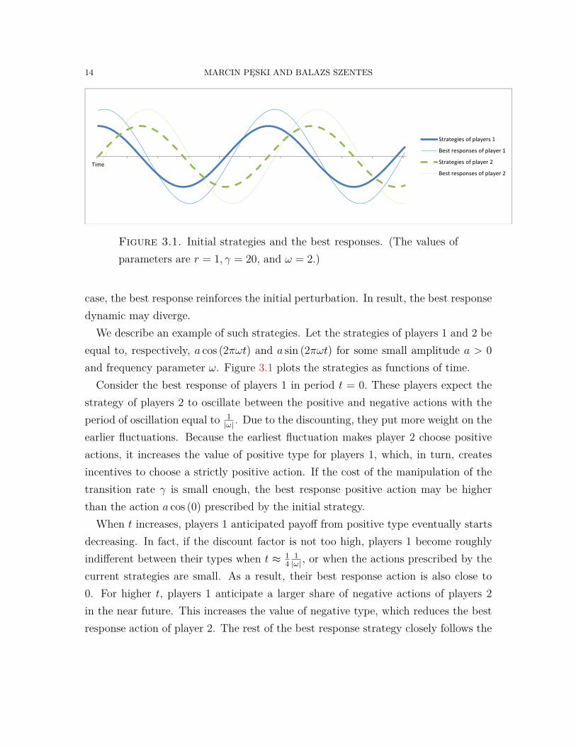
Figure 3.1. Initial strategies and the best responses. (The values ofparameters are r = 1, γ = 20, and ω = 2.)
case, the best response reinforces the initial perturbation. In result, the best responsedynamic may diverge.
We describe an example of such strategies. Let the strategies of players 1 and 2 beequal to, respectively, a cos (2πωt) and a sin (2πωt) for some small amplitude a > 0and frequency parameter ω. Figure 3.1 plots the strategies as functions of time.
Consider the best response of players 1 in period t = 0. These players expect thestrategy of players 2 to oscillate between the positive and negative actions with theperiod of oscillation equal to 1
|ω| . Due to the discounting, they put more weight on theearlier fluctuations. Because the earliest fluctuation makes player 2 choose positiveactions, it increases the value of positive type for players 1, which, in turn, createsincentives to choose a strictly positive action. If the cost of the manipulation of thetransition rate γ is small enough, the best response positive action may be higherthan the action a cos (0) prescribed by the initial strategy.
When t increases, players 1 anticipated payoff from positive type eventually startsdecreasing. In fact, if the discount factor is not too high, players 1 become roughlyindifferent between their types when t ≈ 1
41|ω| , or when the actions prescribed by the
current strategies are small. As a result, their best response action is also close to0. For higher t, players 1 anticipate a larger share of negative actions of players 2in the near future. This increases the value of negative type, which reduces the bestresponse action of player 2. The rest of the best response strategy closely follows the
STABILITY OF STATIONARY EQULIBRIA 15
initial strategy of player 1. (As one can notice on 3.1, the phase of the best responseis shifted relative to the initial strategy. The shift is due to the discounting and itwill disappear when r → 0.)
A similar argument shows that the best responses of player 2 closely resemble thestrategies of player 2. Because the strategies of all players have the same period 1
ω,
the best responses are periodic with the same period length.the cost of non-zero action is relatively low, and its impact on the transition prob-
abilities high. Any small differences between the expected payoffs from negative andpositive types lead to high differences in the best response action. In particular, theamplitude of the best response oscillations can be much higher than the amplitudeof the initial strategies. Because the best response strategies resemble the originalstrategies, one may expect that the best response dynamics lead to ever increasingamplitude of the oscillations, which leads to the divergence of the dynamics.
3.3. Approximate best response dynamics. In order to introduce the main ideasof the paper, we are going to discuss the stability of the best response dynamicsmore carefully. The idea is to derive a linearized approximation to the best responsedynamics, describe the stability of the approximate dynamics, and show that thesame conditions hold for the original best response dynamics.
As a first step, we derive an approximation to the best response function. Let wbe a strategy profile and let v0 be the initial type distribution. Bellman equationsimply that the best response strategy b (σ, v0) must satisfy first-order conditions:
2bt(j, k;σ, v0
)=γ
(V t
(j, 1;w, v0
)− V t
(j,−1;w, v0
)), (3.1)
where Vt (j, k; .) is a period t continuation value of players class j and type 1. Theabove equation has a natural interpretation (compare also with a more general formula(6.3) below). The marginal cost of increasing action bt is equal to 2bt. The marginalbenefit is proportional to the difference between the continuation values of types 1and −1 multiplied by the rate at which an increase in the action affects the rate oftransitions from type −1 to 1.
Next, we compute an approximation to the continuation value function. Because anenvelope theorem applies in our setting, we can approximate the continuation value
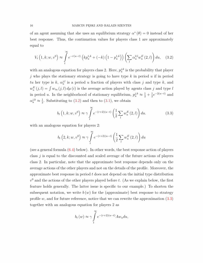
16 MARCIN PĘSKI AND BALAZS SZENTES
of an agent assuming that she uses an equilibrium strategy α∗ (θ) = 0 instead of herbest response. Thus, the continuation values for players class 1 are approximatelyequal to
Vt(1, k;w, v0
)≈
∞
t
e−r(u−t)(kp1,k
u + (−k)(1− p1,k
u
))(∑l
α2,lu w
Eu (2, l)
)du, (3.2)
with an analogous equation for players class 2. Here, pj,ku is the probability that playerj who plays the stationary strategy is going to have type k in period u if in periodtu her type is k, αj,lu is a period u fraction of players with class j and type k, andwEu (j, l) =
´wiu (j, l) dµ (i) is the average action played by agents class j and type l
in period u. In the neighborhood of stationary equilibrium, pj,ku ≈ 12 + 1
2e−2(u−t) and
αj,ku ≈ 12 . Substituting to (3.2) and then to (3.1), we obtain
bt(1, k;w, v0
)≈ γ
∞
t
e−(r+2)(u−t)(
12∑l
wEu (2, l))du. (3.3)
with an analogous equation for players 2:
bt(2, k;w, v0
)≈ γ
∞
t
e−(r+2)(u−t)(
12∑l
wEu (2, l))du
(see a general formula (6.4) below). In other words, the best response action of playersclass j is equal to the discounted and scaled average of the future actions of playersclass 2. In particular, note that the approximate best response depends only on theaverage actions of the other players and not on the details of the profile. Moreover, theapproximate best response in period t does not depend on the initial type distributionv0 and the actions of the other players played before t. (As we explain below, the firstfeature holds generally. The latter issue is specific to our example.) To shorten thesubsequent notation, we write b (w) for the (approximate) best response to strategyprofile w, and for future reference, notice that we can rewrite the approximation (3.3)together with an analogous equation for players 2 as
bt (w) ≈ γ
∞
t
e−(r+2)(u−t)Awudu,

STABILITY OF STATIONARY EQULIBRIA 17
where we treat generalized actions bt (w) and wu as vectors, and A is a matrix equalto
A =
0 0 1
212
0 0 12
12
−12 −
12 0 0
−12 −
12 0 0
.
We can describe an approximation to the best response dynamics. Indeed, supposethat the average strategy in period τ is equal to wτ,E. In particular, the agents planto play action wτ,Et−τ in period t ≥ τ . Between periods τ and τ+dτ , approximately λdτof randomly drawn agents receive a revision opportunity. These agents replace theircurrent strategies by b
(wτ,E
)(we drop the dependence on the initial distribution as
it is not important in our example). Because the agents are chosen at random, theheuristic evolution of the average actions that players intend to play in period t + τ
is given by
dwτ,Et−τdτ
≈ λ(bt−τ
(wτ,E
)− wτ,Et−τ
)(3.4)
≈ λ
γ∞
t−τ
e−(r+2)(u−t+τ)Awτ,Eu du− wτ,Et−τ
for each t ≥ τ.
Because the best responses depend only one the average strategies , the approximatedynamics are well-defined by the above equation. Moreover, due to the approxi-mation (3.3), the right-hand side of the evolution equation is linear in the averagestrategies.where we treat wτ,Et as a vertical vector, and matrix A is defined as follows
3.4. Necessary conditions for stability. Next, we are going to present a necessaryconditions for the stability of the dynamics (3.4). The idea is to consider sine-wavestrategies. It is convenient to describe the sine-way strategies using complex numbers.Specifically, let a = (a (j, k)) be a vector of complex numbers, and let
σat (j, k) =Re (aj,k) cos (2πωt) + Im (aj,k) sin (2πωt) ., (3.5)
=Re(a (j, k) e−i2πωt
)
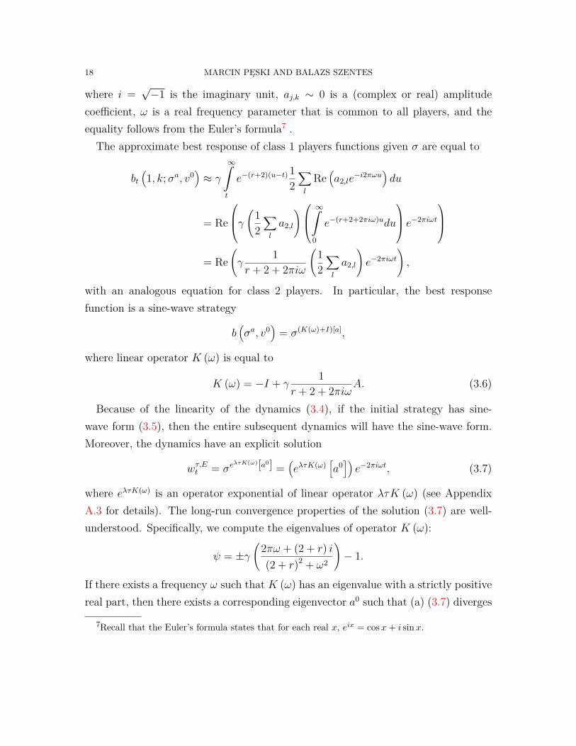
18 MARCIN PĘSKI AND BALAZS SZENTES
where i =√−1 is the imaginary unit, aj,k ∼ 0 is a (complex or real) amplitude
coefficient, ω is a real frequency parameter that is common to all players, and theequality follows from the Euler’s formula7 .
The approximate best response of class 1 players functions given σ are equal to
bt(1, k;σa, v0
)≈ γ
∞
t
e−(r+2)(u−t) 12∑l
Re(a2,le
−i2πωu)du
= Re
γ (12∑l
a2,l
)∞
0
e−(r+2+2πiω)udu
e−2πiωt
= Re
(γ
1r + 2 + 2πiω
(12∑l
a2,l
)e−2πiωt
),
with an analogous equation for class 2 players. In particular, the best responsefunction is a sine-wave strategy
b(σa, v0
)= σ(K(ω)+I)[a],
where linear operator K (ω) is equal to
K (ω) = −I + γ1
r + 2 + 2πiωA. (3.6)
Because of the linearity of the dynamics (3.4), if the initial strategy has sine-wave form (3.5), then the entire subsequent dynamics will have the sine-wave form.Moreover, the dynamics have an explicit solution
wτ,Et = σeλτK(ω)[a0] =
(eλτK(ω)
[a0])e−2πiωt, (3.7)
where eλτK(ω) is an operator exponential of linear operator λτK (ω) (see AppendixA.3 for details). The long-run convergence properties of the solution (3.7) are well-understood. Specifically, we compute the eigenvalues of operator K (ω):
ψ = ±γ(
2πω + (2 + r) i(2 + r)2 + ω2
)− 1.
If there exists a frequency ω such that K (ω) has an eigenvalue with a strictly positivereal part, then there exists a corresponding eigenvector a0 such that (a) (3.7) diverges
7Recall that the Euler’s formula states that for each real x, eix = cosx+ i sin x.
STABILITY OF STATIONARY EQULIBRIA 19
away from 0, and (b) the initial perturbation σa0 leads to a divergent dynamic. Thisgives us a necessary condition for stability.
It turns out that if the real parts of all eigenvalues are strictly negative, then thedynamic is stable regardless of the form of the initial perturbation. The argument issomehow more complicated and we postpone it to Section 6.1.
4. Constants
In this section, we define all the constants that we use in the characterization ofthe stability of stationary equilibria. From now on, we fix the stationary equilibrium(α∗, v∗) of the dynamic game. The subsequent definitions and notations are dividedinto four parts. The first part is devoted to a general terminology on linear operators.The next three parts deal with the constants that are associated with the transitionrates, the payoffs, and the local characterization of the best response function.
4.1. Linear operators. For any two finitely dimensional vector spaces E and E ′,let L (E,E ′) denote the space of linear operators A : E → E ′ with the operator norm‖A‖ = maxe:‖e‖≤1 ‖Ae‖. For example, L (E,R) is the dual space of E. We write L (E)instead of L (E,E). For all operators A,∈ L (E,E ′) and B ∈ L (E ′, E ′′), we writeB A ∈ L (E,E ′′) to denote the composition of A and B.
It will be convenient to extend the definitions of linear operators to vectors spacesover complex numbers. For each vector space E, let EC = E ⊕ iE denote thecomplexification of E.8 Let LC
(EC , E ′C
)be the space of (complex) linear operators
between complex vector spaces EC and E ′C . The standard linear operators betweenvector spaces E and E ′ uniquely extend to (complex) linear operators between EC
and E ′C , i.e., L (E,E ′) ⊆ L(EC , E
′C).9
For any finitely dimensional space E, we say that operator A ∈ L (E) is stable ifeach eigenvalue λ of operator A has strictly negative real part, < (λ) < 0. OperatorA is unstable, if it has an eigenvalue λ with a strictly positive real part, < (λ) > 0.
8In other words, E ⊕ iE = (e1, e2) : ei ∈ E is a vector space with the standard vector additionand multiplication by complex scalar given by (a+ ib) · (e1, e2) = (ae1 − be2, ae2 + be1).
9For any A ∈ L (E,E′), we define ((a+ ib)A) [(e1, e2)] = (aAe1 − bAe2, aAe2 + bAe1).
20 MARCIN PĘSKI AND BALAZS SZENTES
Family of operators B ⊆ L (E) is uniformly stable if there exists γ > 0 such that foreach A ∈ B, each eigenvalue λ of B, < (λ) ≤ −γ.
We assume that |Θ|-dimensional space RΘ and its subspaces ΛΘ and Φ (Θ) areequipped with the “sup” norm. It is convenient to interpret vectors V ∈ RΘ as theelements of the dual spaces L (Φ (Θ) , R) and L (ΛΘ, R) in the natural way: for eachυ ∈ Φ (Θ), let v [υ] = v · υ.
4.2. Transitions. Let γmax <∞ be an upper bound on the absolute values of func-tion γ as well its first, and second-order derivatives.
Let γa;θ,φ, γb;θ,φ ∈ L (A,Φ (Θ)) be the derivatives of function γ : A×Θ×A×Θ→Φ (Θ) with respect to, respectively, a and b (once) evaluated at (α∗ (θ) , θ, α∗ (φ) , φ).
Define linear operators:
• Γ∗ ∈ L (Φ (Θ) ,Φ (Θ)): for each υ ∈ Φ (Θ), let
Γ∗ [υ] =∑θ,φ
γ (α∗ (θ) , θ, α∗ (φ) , φ) υ (θ) v∗ (φ) .
Operator Γ∗ measures the effect of the perturbation in player’s own distri-bution of types on transition rates. The domain of Γ∗ can be extendedto ΛΘ. The stationarity of distribution v∗ implies that Γ∗ [v∗] = 0, andΓ∗ [ΛΘ] ⊆ Φ (Θ),• Γ∗∗Θ ∈ L (Φ (Θ) ,Φ (Θ)): for each υ ∈ Φ (Θ), let
Γ∗∗Θ [υ] =∑θ,φ
γ (α∗ (θ) , θ, α∗ (φ) , φ) v∗ (θ) υ (φ) .
Operator Γ∗∗Θ measures the effect of the perturbation in population on thetransition rates at the stationary distribution,• Γ∗+Θ = Γ∗ + Γ∗∗Θ ∈ L (Φ (Θ) ,Φ (Θ)). Operator Γ∗+Θ measures the combinedeffect of the same perturbation in player’s own distribution and in the generalpopulation,• Γ∗A ∈ L (A, L (Φ (Θ) ,Φ (Θ))): for each generalized action α, each υ ∈ Φ (Θ),
(Γ∗A [α]) [υ] =∑θ,φ
(γa;θ,φ [α (φ)]) υ (θ) v∗ (φ) .
Operator Γ∗A measures the first-order effect of the perturbation in one’s ownactions on the evolution of type distribution,

STABILITY OF STATIONARY EQULIBRIA 21
• Γ∗B : L (A, L (Φ (Θ) ,Φ (Θ))): for each generalized action α, each υ ∈ Φ (Θ),
(Γ∗B [α]) [υ] =∑θ,φ
(γb;θ,φ [α (θ)]) υ (θ) v∗ (φ) .
Operator Γ∗B measures the effect of the perturbation in the population’s ac-tions on the dynamics of the type distribution.• Γ∗A+B = Γ∗A + Γ∗B ∈ L (A, L (Φ (Θ) ,Φ (Θ))). OperatorΓ∗A+B combines twofirst-order effects of the perturbation in actions on the evolution of type dis-tributions,• Γ∗∗A ∈ L (A,Φ (Θ)): for each generalized action α,
Γ∗A [α] =∑θ,φ
(γa;θ,φ [α (φ)]) v∗ (θ) v∗ (φ) .
Operator Γ∗A measures the first-order effect of the perturbation in one’s ownactions on the evolution of type distribution,• Γ∗∗B ∈ L (A,Φ (Θ)): for each generalized action α,
Γ∗A [α] =∑θ,φ
(γa;θ,φ [α (φ)]) v∗ (θ) v∗ (φ) .
Operator Γ∗A measures the first-order effect of the perturbation in one’s ownactions on the evolution of type distribution,• Γ∗A ∈ L
(L (Φ (Θ) , R) , (L (A,R))Θ
): for each vector V ∈ RΘ, each type θ,
((Γ∗A [V ]
)(θ))
[a] =∑φ
(V γa;θ,φ [a]) v∗ (φ) .
Operator Γ∗A measures the impact of the change in the actions on the con-tinuation payoffs V . It plays a role in the characterization of the first orderconditions.
4.3. Payoffs. Let
g∗ =∑
φ
g (α∗ (θ) , θ, α∗ (φ) , φ) v∗ (φ)
be the vector of instantaneous payoffs in the stationary equilibrium.

22 MARCIN PĘSKI AND BALAZS SZENTES
Let V ∗ ∈ RΘ be the value function in the stationary equilibrium. Using the factthat r > 0, we can compute
V ∗ = V (σ∗, v∗) =∞
0
exp (−rt) [g∗ exp (Γ∗t)] dt = g∗ (rI − Γ∗)−1 .
Given our interpretation, we treat g∗ and V ∗ as the elements of the dual spacesL (Φ (Θ) , R) and L (ΛΘ, R).
4.4. Best responses. Define function M : A × Θ × A × Θ → RΘ: so that for allactions a, b and types θ, φ,
M (a, θ, b, φ) = g (a, θ, b, φ) + V ∗ [γ (a, θ, b, φ)] . (4.1)
FunctionM combines two payoff effects of actions: the first term is the direct effect oninstantaneous payoffs g, and the second term captures the effect on the type evolution,which in turn affects the future continuation payoffs. Function M is closely relatedto the terms of the Bellman equation (2.5) and it plays an important role in the localcharacterization of the best response function.
Let M∗a;θ,φ,M
∗b;θ,φ ∈ L
(A,RΘ
)and M∗
aa;θ,φ,M∗ab;θ,φ ∈ L (A,L (A,R)) be the deriva-
tives of function M with respect to, respectively, a (once), b (once), a (twice), and aand b (once each) evaluated at (α∗ (θ) , θ, α∗ (φ) , φ). Define linear operators:
• M∗B ∈ L (A, L (Φ (Θ) , R)) so that for each β ∈ A, each υ ∈ Φ (Θ), we have
(M∗B [β]) (υ) =
∑φ,θ
M∗b;θ,φ [β (φ)] υ (θ) v∗ (φ) ,
Operator M∗B describes the effect of the average change in the population
actions on the equilibrium value of function M ,• M∗
Θ ∈ L(Φ (Θ) , L
(Φ (Θ) , RΘ
)): for each ν, υ ∈ Φ (Θ), each type θ, we have
(M∗Θ [ν]) [υ] (θ) =
∑φ
M (α∗ (θ) , θ, α∗ (φ) , φ) υ (θ) ν (φ) .
OperatorM∗Θ describes the effect of the average change in the population type
distribution on M ,

STABILITY OF STATIONARY EQULIBRIA 23
• M∗AB ∈ L
(A, (L (A,R))Θ
): for each β ∈ A, for each type θ, let
M∗AB [β] (θ) =
∑φ
(M∗
ab;θ,φ [β (θ)])v∗ (φ) .
(Notice that that the derivative Ma with respect to a can be treated as anelement of the vector space A, and that M∗
ab;θ,φ can be understood as a linearoperator on A.) OperatorM∗
AB captures the effect of the change in the averageaction in the environment β on the equilibrium first-order conditions,• M∗
AΘ ∈ L(Φ (Θ) , (L (A,R))Θ
): for each υ ∈ Φ (Θ), for each type θ, let
M∗AΘ [υ] (θ) =
∑φ
M∗a;θ,φυ (φ) .
Operator M∗AΘ captures the effect of the change in the average type on the
equilibrium first-order conditions,• M∗
AA ∈ L(A, (L (A,R))Θ
): for each α ∈ A, for each type θ, let
(M∗AA [α]) (θ) =
∑φ
(M∗
aa;θ,φ [α (θ)])v∗ (φ) .
We show below that the stationary equilibrium conditions imply that operatorM∗
AA is negatively semi-definite. If M∗AA is negative definite, it has an inverse
M−1AA ∈ L
((L (A,R))Θ ,A
).
5. Stability of type distribution
Our first result characterizes the stability of the type distribution dynamics withrespect to initial perturbation of the type distribution away from the stationary dis-tribution v∗.
Theorem 1. Suppose that linear operator Γ∗ is stable. If operator Γ∗+Θ is stable,then the type distribution is stable at the stationary equilibrium. If operator Γ∗+Θ isunstable, then the type distribution is unstable.
The Theorem assumes that the eigenvalues of Γ∗ have strictly negative real parts(notice that the real parts of the eigenvalues of Γ∗ are always non-positive because Γ∗
is a stochastic matrix). If operator Γ∗+Θ is stable, then all (sufficiently small) initialperturbations in the type distributions disappear in the long-run. If the operator Γ∗+Θ

24 MARCIN PĘSKI AND BALAZS SZENTES
is unstable, then we can find an arbitrarily small initial perturbation v0 that leads tothe diverging dynamics.
We sketch an argument behind Theorem 1. Take any υ0 ∈ Φ (Θ) and let v0c =v∗+υ0 for each cohort c. Because all cohorts behave in the same way, we may assumethat there is only one representative cohort. The type distribution evolves accordingto the following differential equation
d
dtvt =
∑θ,φ
γ (α∗ (θ) , θ, α∗ (φ) , φ) vt (φ) vt (θ) for each t ≥ 0, (5.1)
with initial conditions v0 = v∗ + υ0.Equation (5.1) typically does not have a closed-form solution and we consider a
linearized approximation. Notice that for each t ≥ 0,d
dtvt =
∑θ,φ
γ (α∗ (θ) , θ, α∗ (φ) , φ) vt (φ) vt (θ)
=∑θ,φ
γ (α∗ (θ) , θ, α∗ (φ) , φ) v∗ (φ) v∗ (θ)
+∑θ,φ
γ (α∗ (θ) , θ, α∗ (φ) , φ) (v∗ (φ) (vt (θ)− v∗ (θ)) + (v∗t (φ)− v∗ (φ)) v∗ (θ))
+∑θ,φ
γ (α∗ (θ) , θ, α∗ (φ) , φ) ((vt (θ)− v∗ (θ)) (v∗ (φ)− v∗ (φ)))
≈∑θ,φ
γ (α∗ (θ) , θ, α∗ (φ) , φ) (v∗ (φ) υt (θ) + υt (φ) v∗ (θ)) = Γ∗+Θ [υt] ,
where the approximate equality comes from the fact that the first term disappearsbecause v∗ is a stationary distribution, and the last term is of second-order magnitude.The linearized equation has a closed-form solution
vt ≈ v0 + exp(tΓ∗+Θ
)(v0 − v∗) ,
where exp (.) is the matrix exponential function (see Appendix A.3for details).By the properties of the matrix exponential, if operator Γ∗+Θ is stable, then
limt
∥∥∥exp(tΓ∗+Θ
)υ0
∥∥∥ = 0
for any initial υ0 = v0 − v∗. If it is unstable, then there exists an eigenvector υ0 ofΓ∗+Θ such that limt
∥∥∥exp(tΓ∗+Θ
)υ0
∥∥∥ =∞. In particular, the solution to the linearized

STABILITY OF STATIONARY EQULIBRIA 25
equation diverges. Appendix E shows that the instability of the solution extends tothe original equation (5.1 ).
6. Stability of stationary equilibria with respect to best responsedynamic
In this section, we describe the sufficient and (almost) necessary conditions for thestability of stationary equilibria with respect to the best response dynamics.
Suppose that operator matrix M∗AA is negative semi-definite and operators Γ∗ and
Γ∗+Θ are stable. Then, for each ω ∈ R, (complex) linear operators
M∗AA, 2πiωIΦ(Θ) − Γ∗+Θ, (r + 2πiω) IΦ(Θ) − Γ∗
have well-defined inverses. Define a family of (complex) operatorsK (ω) ∈ LC(AC,AC
):
for each α ∈ A,
(K (ω)) [α] (6.1)
=− IA −M−1AA M∗
AB [α]
−M−1AA M∗
AΘ (2πiωIΦ(Θ) − Γ∗+Θ
)−1(Γ∗A+B [α]
)−M−1
AA Γ∗A (M∗B [α])
((r + 2πiω) IΦ(Θ) − Γ∗
)−1
−M−1AA Γ∗A
(M∗
Θ
[(2πiωIΦ(Θ) − Γ∗+Θ
)−1(Γ∗A+B [α]
)])((r + 2πiω) IΦ(Θ) − Γ∗
)−1.
Theorem 2. Suppose that operator M∗AA is negative definite and operators Γ∗ and
Γ∗+Θ are stable. If family K (ω) is uniformly stable, then there exists λ∗ > 0 such thatfor each λ < λ∗, the stationary equilibrium is λ-stable. If there exists ω such thatK (ω) is unstable, then the stationary equilibrium is λ-unstable for any λ.If family K (ω) : ω ∈ Ω is uniformly stable, then there exists λ∗ > 0 such that foreach λ < λ∗, the stationary equilibrium is (Ω, λ)-stable. If there exists ω ∈ Ω suchthat K (ω) is unstable, then the stationary equilibrium is (Ω, λ)-unstable for any λ.
The Theorem provides a sufficient and almost necessary condition of the stability ofstationary equilibrium. In order to verify the conditions, one needs to find eigenvaluesof a one-dimensional family of linear operators K (ω).
26 MARCIN PĘSKI AND BALAZS SZENTES
The Theorem requires three assumptions. The two first assumptions are not re-strictive. First, a local characterization of stationary equilibrium (see Lemma 1 andstep 2 of the proof of Lemma 12 in the Appendix) implies that operator M∗
AA is al-ways negative semi-definite. The Theorem makes a slightly stronger assumption thatoperator M∗
AA is negative definite. Second, noticeΓ∗ that always has eigenvalues withnon-positive real part because it is a stochastic operator. The Theorem assumes thatthe eigenvalues of Γ∗ have strictly negative real parts. Finally, the only restrictiveassumption is that that Γ∗+Θ is stable. However, as we have already demonstrated,together with the stability of Γ∗, this assumption is sufficient and almost necessaryfor the stability of the evolution of the type distribution (Theorem 1). Together, theassumptions of the Theorem ensure that the best response strategy is uniquely de-fined for profiles of strategies and initial distributions that are in some neighborhoodof the stationary equilibrium values.
It is instructive to compare Theorem 2 with an analogous result in the case ofstatic games. Recall that a static game equilibrium is stable if all eigenvalues of theJacobian of the best response function computed at the equilibrium have real partsthat are strictly smaller than 1. In the case of dynamic games, the space of strategiesis infinitely dimensional and it would not be possible (or helpful) to state the result interms of a “derivative” of the best response function. However, each linear operatorK (ω) + IA can be interpreted as the Jacobian of the best response function restrictedto a finitely dimensional class of wave-like strategies with frequency ω. Specifically,consider a class of strategies σ (ω, α) indexed by a (real) frequency parameter ω ∈ Rand a (complex) amplitude vector α ∈ AC :
σt (θ;ω, α) =σ∗t + Re(α (θ) e−i2πωt
). (6.2)
=σ∗t + Re (α (θ)) cos (−2πωt)− Im (α (θ)) sin (−2πωt) .
The second equality comes from the Euler’s formula (see footnote 7). If ω = 0, thenσ (ω, α) is a constant strategy; otherwise, it is periodic with period length 1
ω. The am-
plitude vector contains information about the generalized actions played throughoutthe wave-like strategy and also about the phase of the strategy. Its norm, ‖α‖, mea-sures the deviation of strategy σ (ω, α) away from the stationary strategy σ∗. Below
STABILITY OF STATIONARY EQULIBRIA 27
(see equation (6.3)), we argue that if a population of players uses strategy σ (ω, α)with sufficiently small vector α, then the best response strategy belongs to wave-likeclass with frequency ω: for high t,
bt (σ, v0) ≈ σ (ω, (K (ω) + IA)α)
(We explain below that for high t, the best response does not depend on the initialdistribution v0. ) Thus, linear operator K (ω) + IA contains an information aboutthe link between an amplitude vector of a wave-like strategy, and the amplitude ofthe best response.
A consequence of the proof of the Theorem is that to test the stability it is notnecessary to consider all possible initial perturbations, and it is enough to restrict theanalysis to a class wave-like perturbations of form (6.2).
The proof of the Theorem is based on ideas similar to those that are developed inSections 3.3-??. We sketch key steps below and leave the details for the Appendix.
6.1. Sketch of the proof of Theorem 2: sufficient conditions. We explain theargument behind the first part of the Theorem. The idea is to derive a stability test fora simplified version of the best response dynamics and then show that the same testapplies to the original dynamics. . We proceed through a series of approximations.The first step is to find a linear approximation to the best response function.
Approximation of the best response function. Take a profile of strategies w and aprofile of initial type distributions v0. We are going to show that we can approximatebt (w, v) in the neighborhood of the stationary equilibrium with a linear function ofw and v0. As an intermediary step, we use Lemma 1 and notation from Section 4 toshow that
bA0t (w, v0)− σ∗t ≈−M−1
AA M∗AB
[wEt − α∗
](6.3)
−M−1AA M∗
AΘ
[vEt (w, v0)− v∗
]−M−1
AA Γ∗A [Vt (w, v0)− V ] .
28 MARCIN PĘSKI AND BALAZS SZENTES
(For details, see step 2 of the proof of Lemma 12 in Appendix D.) In particular, thet-period best responses depend on the average actions played in the population, theaverage type distributions, and the value functions in period t.
It is instructive to notice that the terms of the approximation (6.3) with the termsof linear operator K (ω).
As a next step, we derive linear approximations to the evolution of the type dis-tribution vEt (w, v0) and the value function Vt (w, v0). The former depends on theactions played before period t and the initial distribution v0 for details, see Lemma9 in Appendix C). The latter depends on the actions played after period t, and thetype distributions in periods s > t, which in turn depend on the actions played beforeperiod s and the initial distribution v0 (see step 4 of Lemma 12 in Appendix D).As we do not have closed-form formulas for the two approximations, we delay theirformal statement to the Appendix. Using the approximations together with (6.3), weshow that that there exists a (real) operator valued function κ : R → L (A,A) suchthat for all profiles w of strategies and v0 of initial type distributions, for high t,
bt (w, v0)− σ∗t ≈ −(M−1
AA M∗AB
) [wEt − α∗
]+
∞
−∞
κ (u)[wEt−u − σ∗
]du. (6.4)
(To simplify the notation, we assume that wEu = σ∗u for each u ≤ 0.) In particular,the best response is approximately equal to the weighted average of the present, pastand future average actions in the population. Notice that the right-hand side of (6.4)does not depend on the initial distribution v0. This is because of the ergodicity ofthe evolution of types (more precisely, due to the stability of linear operators Γ∗ andΓ∗+Θ), the effect of the initial distribution disappears for high t.
The operator-valued function κ (u) aggregates the past (for positive u) and future(for negative u) actions. For further use, it is important to describe two propertiesof κ (.). First, κ (.) has exponentially decaying tails, i.e., ‖κ (u)‖ ≤ Peρu for someconstants P and ρ. The interpretation is that the impact of actions far away in thefuture or in the past on the present best response action decays exponentially. Second,although we do not have a closed-form formula for κ, we can show that its Fourier

STABILITY OF STATIONARY EQULIBRIA 29
transform10 is equal to
Fκ (ω) =∞
−∞
e2πiωuκ (u) du = K (ω) + IA +M−1AA M∗
AB, (6.5)
where linear operator K (ω) is defined in (6.1).
Approximate linear dynamics. Let (wτ , vτ ) be the best response dynamics initiatedby perturbation (w0, v0). For each t > τ , define a generalized action
$τt = wτ,Et−τ − α∗ =
ˆ (wτc,t−τ − α∗
)dµλ (c) .
Thus, $τt is equal to the difference between the average action that τ -period agents
plan to play in period t > τ and the stationary equilibrium action.We are going to describe the dynamics of $τ
t . Recall that the average action $τt
changes with τ because in each period τ , a fraction of players replace their strategiesby the best response b (wτ , vτ ). Because the arrival of a revision opportunity is inde-pendent from the agents’ behavior, and because the mass of the players that receivethe revision opportunity is equal to λdτ , the change in the average action is equal to
d$τt
dτ= λ (bt−τ (wτ , vτ )−$τ
t ) for t ≥ τ. (6.6)
We use approximation (6.4) to derive a linearized version of the above dynamics:for t ≥ τ ,
d$τt
dτ≈ λ
(−IA −M−1AA M∗
AB
)[$τ
t ] +∞
−∞
κ (u)[$τt−u
]du
. (6.7)
We need to be careful here because approximation (6.4) is only valid for high t.However, it turns out that, if λ is sufficiently low, the approximation (6.4) is goodenough. The intuition is that if the revision opportunities are rare, then from thepoint of view of period t, the bulk of actions played in period t were chosen as thebest responses in periods s t and they are well approximated by (6.4).
The dynamics (6.7) are still too complicated for a head-on analysis. We make twoadditional simplifications. First, suppose that actions $τ
t and equation (6.7) holdsfor all all t, including t ≤ τ . Second, suppose that $0
t is square-integrable in t. In10See Appendix A.2 for the formal definition and the properties of the Fourier transform.

30 MARCIN PĘSKI AND BALAZS SZENTES
what follows, we first analyze the dynamics (6.7) with the two simplifications, andnext, we explain how to dispense with them.
Dynamics of Fourier coefficients. The two assumptions imply that $τt can be treated
as square-integrable functions of t ∈ R. In particular, we can apply Fourier transformto the both sides of (6.7): for each ω ∈ R,
dF$τ (ω)dτ
=F(d$τ
.
dτ
)(ω)
=F
λ(−IA −M−1
AA M∗AB
)[$τ
. ] +∞
−∞
κ (u)[$τ.−u
]du
(ω)
=λ((−IA −M−1
AA M∗AB
)[F$τ (ω)] + Fκ [F$τ (ω)]
)=λK (ω) [F$τ (ω)] . (6.8)
The first and the third equality follows from the linearity of the Fourier transform.The last equality comes from (6.5).
Equation (6.8) is a linear time-homogeneous first-order (vector-valued) differentialequation that can be analyzed separately for each ω and it has an explicit solution
F$τ (ω) = etλK(ω)[F$0 (ω)
], (6.9)
where etλK(ω) is a matrix exponential function.11
The convergence properties of (6.9) are well-understood. In particular, if the realparts of all eigenvalues of operators K (ω) are uniformly bounded away from 0, thenF$τ (ω)→ 0 when τ →∞ at exponential rate.
Back to the original dynamics. Because the Fourier transform has a continuous in-verse, the convergence of the Fourier coefficients F$τ (ω) implies that the averageactions converge to 0. (We gloss over some technical issues: The convergence ofFourier coefficients implies the convergence of $τ (ω) → 0 in the square-integrablenorm L2. An additional argument is required to show that the average actions con-verge to 0 uniformly, or that $τ (ω) → 0 in the “sup”, L∞-norm. That argumentrelies on the fact that function κ is uniformly bounded and has exponential tails.)
11See Appendix A.3 for details.

STABILITY OF STATIONARY EQULIBRIA 31
We briefly discuss the issues related to extending the convergence of the linearizeddynamics (6.7) to the original dynamics. First, we want to show that the convergenceholds for all functions $τ
t uniformly bounded (in t) and not only square-integrable.For this purpose, for each t, we take some sufficiently large ∆ > 0 and divide the ini-tial perturbation $0 into two parts $0 = $0,near t +$0,distant t , where $0,near t =$0s1|s−t|≤∆ corresponds to near past and future, and $0,distant t = $0
s1|s−t|>∆ corre-sponds to distant past and future. Because (6.7) is linear, we can separately considerthe dynamics initiated by each of the two parts. The “near” part is square integrable,hence the dynamics converges by the above argument. The speed of the convergencedepends on the square-norm of $0,near t, hence it decreases with ∆. Because of theexponentially decaying tails of function κ, the effect of the distant part on the dy-namics of $τ
t is limited as long as τ < τ ∗ for some threshold τ ∗ that increases with ∆.We can choose ∆ so to guarantee that
∥∥∥$τ∗t
∥∥∥ is smaller than ‖$0t ‖ uniformly across
all t. We repeat the argument to show that $τt → 0 uniformly across all t.
Second, we want to show that the convergence holds if the average actions $τt and
th, A profile w (ω, α) of wave-like strategies is characterized by (unique) frequencyparameter ω and a measurable function α : C → AC that assigns an amplitude to eachcohort. e dynamics (6.7) are restricted to τ ≤ t. As compared to the linearized versionof the original dynamics, the unrestricted dynamics contains an error that comes fromthe evolution of actions $τ
t for t ≤ τ . It turns out if the revision opportunities arevery rare, then the error has a very limited impact on the evolution of actions $τ
t fort > τ , i.e., the part covered by the restricted dynamics. The idea is that
Finally, we bound the difference between the best response dynamic and its lin-earized version using similar arguments to those used in the analysis of the revisiondynamics in the case of static games.
6.2. Sketch of the proof of Theorem 2: necessary conditions. We explainthat if operator K (ω) has an eigenvalue with a positive real part, then there existsan initial perturbation of a particular wave-like form that initiates diverging bestresponse dynamic. The argument relies on the approximation methods developed inthe first part of the proof.
32 MARCIN PĘSKI AND BALAZS SZENTES
For each frequency ω ∈ R and measurable function α : C → AC , define a profile ofwave-like strategies so that for each cohort,
wc (ω, α) = σ (ω, α (c)) ,
where σ (ω, α (c)) is a wave-like strategy with frequency ω and amplitude α (c) thatis defined above in (6.2). Let αE =
´α (c) dµλ (c) be the average amplitude in profile
w (ω, α).We use (6.4) to compute an approximate best response to wave-like profiles w
(ω, αC
):
bt (w (ω, α) , .) ≈−(M−1
AA M∗AB
) [Re
(αEe−i2πωt
)](6.10)
+∞
−∞
κ (u)[Re
(αC,Ee−i2πω(t−u)
)]du
=Re((−(M−1
AA M∗AB
) [αE]
+ Fκ (ω)[αC,E
])e−i2πωt
)=σ
(ω, (K (ω) + IA)
[αE]).
(The first proper equality comes from the fact that linear operators M−1AA,M
∗AB, and
the operator-valued function κ have only real parts, and from the definition of theFourier transform.) In particular, the best response has a wave-like form with thesame frequency parameter as the original strategy profile. The amplitude coefficientof the best response strategy is a linear function of the average amplitude in thepopulation. The exact value is determined by on the is equal to to the value ofoperator K (ω) on the amplitude of the original strategy.
We explain how to use observation (6.10) to show the instability of the best responsedynamics. Suppose that the τ -period strategy in the population is given by profilew (ω, ατ ) with the average amplitude αE,τ . The τ -period best response strategy isgiven by (6.10). During the next dτ periods, a fraction λdτ of players receives anopportunity to revise their strategies to the best response strategy. In particular,after dτ periods, the new population profile has the same form as the original profilebut with a slightly different distributions of amplitudes with the average amplitudeapproximately equal to
αE,τ+dτ = (1− λdτ)αE,τ + λdτ (K (ω) + IA)[αEτ
]. (6.11)

STABILITY OF STATIONARY EQULIBRIA 33
Because the (approximate) best responses depend only on the average amplitude,we can trace the behavior of the best response dynamics by tracing the behavior ofthe average amplitudes. Heuristics (6.11) suggests that the average amplitude evolvesaccording to the linear, time-homogenous differential equation
dαEτ
dτ= K (ω)
[αEτ
].
The long-run behavior of such equations is well-understood and it depends on theeigenvalues of operator K (ω). If α∗ is a (possibly, complex) eigenvector of K (ω)with a (possibly, complex) eigenvalue ψ, then
αEτ = eψτα∗
is a solution to the above differential equation. If ψ has a strictly positive real part,then the above solution explodes and the approximate linearized dynamic diverges.We extend
7. Stability of stationary equilibria with respect to learningdynamic
In this section, we describe the sufficient and (almost) necessary conditions for thestability of stationary equilibria with respect to the learning dynamic.
Theorem 3. Suppose that operator M∗AA is negative semi-definite and operators Γ∗
and Γ∗+Θ are stable. Take any finite set Ω ⊆ R, 0 ∈ Ω of frequencies. If familyK (ω) : ω ∈ Ω is uniformly stable, then there exists λ∗ > 0 such that for each λ <λ∗, the stationary equilibrium is (Ω, λ)-stable. If there exists ω ∈ Ω such that K (ω) isunstable, then there exists λ∗ > 0 such that for each λ < λ∗, the stationary equilibriumis (Ω, λ)-unstable.
The Theorem says that the uniform stability of family K (ω) : ω ∈ Ω is a sufficientand almost necessary condition of the stability of stationary equilibrium.
As we explained in the discussion of Theorem 3, each operator K (ω) is a Jacobianof the best response function restricted to strategies that have wave-like form withfrequency ω. The fact that it is enough consider wave-like strategies is not surprising

34 MARCIN PĘSKI AND BALAZS SZENTES
given that the learning dynamics force the agents to predict wave-like strategies oftheir the opponents.
The learning dynamic encompasses variety of models that differ with respect to therange of frequencies Ω that can be detected by the agents. The Theorem implies thatthe larger detectable set Ω, the more stringent conditions required for the stability ofequilibrium. The intuition is that if the agents can detect more patterns, this leadsto more complicated dynamics, with extra possibilities for instability.
7.1. Sketch of the proof. As in the case of the best response dynamics, the proofof Theorem 3 relies on the linearization of the learning dynamic in the neighborhoodof the stationary equilibrium. The details differ somewhat from the proof of Theorem2. We sketch the main idea below.
Suppose that family K (ω) : ω ∈ Ω is uniformly stable. We are going to arguethat for each strategy profile w in a (sufficiently small) neighborhood of the stationaryequilibrium, the average coefficients at,Ecos (.) and at,Esin (.) of regression (2.7) converge to0. This implies the convergence of the best responses, as well as the convergence ofthe dynamics.
It is convenient to define “Fourier” decomposition of the average past actions: foreach frequency ω, and for t,
aEt (ω) = 2t
tˆ
0
(ws,E0 − α∗
)ei2πωsds. (7.1)
The complex coefficient aEt (ω) is closely related to the regression coefficients: forsufficiently large t, and all ω 6= 0,
aEt (ω) ≈at,Ecos (ω) + iat,Esin (ω) .
We also have at,Ecos (0) ≈ α∗ + Re(aEt (0)
)(because sin (0) = 0, the value of the coeffi-
cient at,Esin (0) is not important). The approximations follow from the Euler’s formulaand the equations that characterize the linear regression. Due to the approximations,

STABILITY OF STATIONARY EQULIBRIA 35
the agents forecast made in period t is (approximately) equal to
wP,t,Es−t =∑ω′∈Ω
at,Ecos (ω′) cos (2πω′s) + at,Esin (ω′) sin (2πω′s) (7.2)
≈∑ω′∈Ω
Re(aEt (ω′) e−i2πω′s
).
In particular, the forecast has a wave-like form (6.2).We are going to describe the dynamics of the coefficients aEt (.). Notice that the
average actions played in period s are equal to a (weighted) average of the actionsplanned in period 0 and the best responses chosen by players who revised the strategiesbetween periods 0 and s:
ws,E0 = e−λsw0,Es + λ
sˆ
0
bs−u(wP,u, vu
)e−λ(s−u)du.
The weights on different periods depend on the arrival rate λ of revision opportunities.Because the first term becomes small for sufficiently large s, we are going to drop it insubsequent calculations. We can approximate the best response action using formula(6.10) as well as the approximation of the forecasted strategy (7.2):
bs−u(wP,u, vu
)− α∗ ≈
∑ω′∈Ω
Re((K (ω′) + IA)
[aEu (ω′)
]e−i2πω
′s).
We substitute the two above equations into (7.1): after some algebra, we obtain asequence of approximations:
aEt (ω) ≈ 2t
tˆ
0
∑ω′∈Ω
Re
(K (ω′) + IA)
λsˆ
0
([aEu (ω′)
])e−λ(s−u)du
e−i2πω′s ei2πωsds
≈ 2t
tˆ
0
∑ω′∈Ω
Re((K (ω′) + IA)
[aEs (ω′)
]e−i2πω
′s)ei2πωsds
≈ 2t
tˆ
0
Re((K (ω) + IA)
[aEs (ω′)
]e−i2πωs
)ei2πωsds
≈ 1t
tˆ
0
(K (ω) + IA)[aEs (ω′)
]ds

36 MARCIN PĘSKI AND BALAZS SZENTES
(In the second line, we use the fact that λ´ s
0
([aEu (ω′)
])e−λ(s−u) ≈ aEs (ω′) for each
frequency ω′. In the third line, we use the fact that an integral of a product of twowave-like functions with different frequencies ω′ 6= ω is close to 0. The last line relieson an analogous fact about the integral of the product of imaginary exponential withthe real part of wave-like strategy with the same frequency ω. )
The last line of the above equation describes an approximate dynamics of theFourier coefficients. (Notice the similarity to fictitious play formula). The approxi-mate dynamics has a closed-form “solution”
aEt (ω) = e(log t)K(ω)aE0 (ω) .
As we discuss above, the approximate “ solution” converges if linear operator K (ω)is stable. It diverges if K (ω) is unstable, and aE0 (ω) is chosen to be the eigenvectorassociated with an eigenvalue of K (ω) with a strictly positive real part.
8. Conclusions
TBA
ReferencesAppendix A. Mathematical Preliminaries
A.1. Terminology and notation. For each Banach space X, each profile of X-valued paths χ ∈ D
((C, C, µ)X
), define the real valued paths χE, ‖χ‖. ∈ X, so that
for each t,
χEt =ˆχ (c) dµ (c) , and
‖χ‖t = ‖χ (., t)‖L2 =√ˆ‖χ (c, t)‖2 dµ (c).
Recall that Lp (R,E) for each 1 ≤ p ≤ ∞ is the space of Lebesgue-measurable,Lp-integrable functions g : R→ E. We denote the Lp-norm of function g ∈ Lp (R,E)as ‖g‖Lp .
A Lebesgue-measurable function g : R → E is exponentially bounded if thereexists constants P < ∞ and ρ > 0 such that for each t ∈ R, ‖g (t)‖ ≤ Pe−ρ|t|. Let

STABILITY OF STATIONARY EQULIBRIA 37
Lexp (R,E) be the space of exponentially bounded functions. Of course, Lexp (R,E) ⊆Lp (R,E) for each 1 ≤ p ≤ ∞.
It is convenient to introduce the following terminology: For any two functionsζ (w, v0) , ξ (w, v0) ∈ X that depend on profiles of strategies w and initial type dis-tributions v0 and with the values in some Banach space X, we say that ζ is a first(or second)-order approximation for ξ, if there exist constants K < ∞ and ε > 0that depend only on the parameters of the model (i.e., the values and derivatives offunctions g and γ), for all profiles of strategies w and initial type distributions v0 suchthat ‖w − σ∗‖+ ‖v0 − v∗‖ ≤ ε,
‖ζ (w, v0)− ξ (w, v0)‖X ≤ K (‖w − σ∗‖+ ‖v0 − v∗‖) ,(or ‖ζ (w, v0)− ξ (w, v0)‖X ≤ K (‖w − σ∗‖+ ‖v0 − v∗‖)2
).
A.2. Convolutions and Fourier transforms. For each κ ∈ L1 (R,B (E)) and eachh ∈ Lp (R,E), define convolution κ ? h : R→ E as
(κ ? h) (t) =∞
−∞
κ (t− s) [h (s)] ds.
Notice that ‖κ ? h‖Lp ≤ ‖κ‖L1 ‖h‖LP . We can check that if κ ∈ Lexp (R,B (E ′, E ′′))and h ∈ Lexp (R,B (E,E ′)), then κ ? h ∈∈ Lexp (R,E).
For each h ∈ L1 (R,E), define the Fourier transform of h as Fh : R→ E,
Fh (ω) = h (ω) =∞
−∞
h (t) e−2πitωdt.
LetR be the “flip” operator, i.e.,Rh (x) = h (−x). If functions h and h are integrable,then the Fourier transform is equal to its inverse modulo the flip:
F−1 (RF (h)) = F−1 (FR (h)) = h. (A.1)
If h ∈ L1 (R,E) ∩ L2 (R,E), then the Plancherel’s Theorem implies that
‖h‖L2 =∥∥∥h∥∥∥
L2. (A.2)
Also, we have ‖Fh‖L∞ ≤ ‖h‖L1 .
38 MARCIN PĘSKI AND BALAZS SZENTES
For any κ ∈ Lexp (R,B (E)) and h ∈ L1 (R,E), the convolution theorem says thatthe Fourier transform of the convolution κ ? h is equal to the product of the Fouriertransforms of κ and h,
F (κ ? h) (ω) = F (κ) (ω) [F (h) (ω)] . (A.3)
A.3. Matrix and operator exponential. Let X be a finitely dimensional vectorspace. For each A ∈ L (X,X), and each t, define linear operator exp (A) ∈ L (X,X)as
exp (A) =∞∑n=0
1n! (A)n . (A.4)
We refer to exp (A) as the matrix exponential. It is well-known that if linear operatorA is stable, then limt→0 e
tA = 0, and if Ais unstable, then there exists v0 ∈ X suchthat limt→0
∥∥∥etAv0
∥∥∥ =∞. We use the following uniform version of this result.
Lemma 2. Suppose that X is a finitely dimensional vector space. Suppose that familyof operators B ⊆ L (X,X) is relatively compact (i.e., its closure is a compact set)and uniformly stable. Then, there exists P <∞ and ρ > 0 such that for each A ∈ B,each x ∈ X, each t ≥ 0,
‖exp (At)x‖ < Pe−ρt ‖x‖ .
Proof. The claim follows from the continuity of eigenvalues.
The definition of the matrix exponential can be generalized to bounded linearoperators on Banach spaces. Let X be a Banach space, and let L (X,X) be thespace of bounded linear operators A : X → X with the operator norm ‖A‖ =supx:‖x‖≤1 ‖Ax‖. We can define the operator exponential using formula (A.4). Then,exp (A) is a well-defined, bounded, linear operator. Moreover, ‖exp (A)‖ ≤ e‖A‖, andfor each x ∈ X, xt = exp (At)x is the unique solution to the differential equation
dxtdt
= Axt
with initial conditions x0 = x.
Lemma 3. Suppose that A is a bounded linear operator on Banach space X. Then,there exists limit
ρA = limt→∞
1t
log ‖exp (At)‖ .

STABILITY OF STATIONARY EQULIBRIA 39
Moreover, for each η > 0,
• there is a constant Pη,A <∞ such that for each x ∈ X and t,
‖exp (At)x‖ ≤ Pe(ρA+η|ρA|)t ‖x‖ , and
• for each t ≥ 0, there exists x ∈ X such that
‖exp (At)x‖ ≥ e(ρA−η|ρA|)t ‖x‖ .
Remark 1. If X is finitely dimensional, then ρA is equal to the largest real part ofeigenvalues of matrix A.
ρA = max Re (λ) : λ is an eigenvalue of X .
Proof. For each t, let ρt = 1t
log ‖exp (At)‖. Function ρ. is continuous with t andbounded by ‖A‖. Moreover, for each s > t > 0,
ρs ≤(
1 + 1bs/tc
t
)ρt.
It follows that for each t, γt ≥ lim supt→∞ γs, and that there exist limit γA =limt→∞ γt.
Fix η > 0. Let Pη,A = supt t (ρt − (ρA + η |ρA|)). Then, PA < ∞ because ofcontinuity of ρ., its boundedness, and the existence of the limit and part (a) holds.Additionally, for each t, there exists x ∈ X such that ‖exp (At)x‖ ≥ e(ρA−η|ρA|)t ‖x‖.Because ρt ≥ ρA, part (b) follows.
A.4. Lyapunov functions on finitely dimensional spaces. The next result de-scribes Lyapunov-type functions for stable and unstable linear operators finitely di-mensional space X. Recall the a set X ′ ⊆ X is a cone if for each x ∈ X ′, eachλ ∈ R,λx ∈ X ′. For each cone X ′, say that continuous y : X ′ → R+ is a cone function, ify (x) = 0 for x ∈ X ′ iff x = 0 and such that y (λx) = |λ| y (x).
Lemma 4. Suppose that X is a finitely dimensional (complex) vector space and A ∈L (X,X).
(1) If A is stable, then there exists a cone function yA : X → R such that for eachx 6= 0, yA (x) > 0, yA (x) is differentiable, and ∇yA (x) · Ax < 0.

40 MARCIN PĘSKI AND BALAZS SZENTES
(2) If A is unstable, then there exists a cone XA ⊆ X, a cone function yA :XA → R+, and constants η, ρ > 0 such that for each x ∈ XA, each ε ∈ X, if‖ε‖ ≤ η ‖x‖, then for each d > 0
Ax+ ε ∈ XA and yA (x+ d (Ax+ ε))− y (x) ≥ ρd ‖x‖ .
Proof. Part 1. Let
yA (x) =∞
0
‖exp (At)x‖ dt.
Part 2. Let
A =
J1
J2
...
Jn
be the Jordan decomposition of operator A, let λi be the eigenvalue associated withblock matrix Ji, and let e =
(e1
1, ..., e1m1 , ..., e
nmn
)be the associated basis. For each x,
let(x1
1, ..., x1m1 , ..., x
nmn
)denote the representation of vector x in the basis. Then,
Ji
xi1
xi2
...
xini
=
λix
i1 + xi2
λixi2 + xi3
...
λixin
.
Let I be the set of eigenvalues such that Re(λi) > 0. Because operator A is unstable,set I is nonempty. For each i ∈ I, let wi1 = 1, and, recursively, wik+1 = 2
Re(λi)wik for
each k = 1, ...,mi − 1.For each x, define
yA (x) = maxi∈I
maxm≤mi
wi∣∣∣xim∣∣∣ ,
y′ (x) =∑j /∈I,m
∣∣∣xjmj ∣∣∣ .Define cone
XA =x :
(mini∈I
Re (λi))yA (x) ≥ 8y′ (x)
.
Then, for each x ∈ XA, yA (x) ≥ µ ‖x‖ for some constant µ > 0.
STABILITY OF STATIONARY EQULIBRIA 41
Notice that for each i ∈ I,
wim∣∣∣(1 + dλi)xim + dxim+1
∣∣∣ ≥wim ∣∣∣xim∣∣∣+ dwim(Re (λi)
∣∣∣xim∣∣∣− ∣∣∣xim+1
∣∣∣)≥wim
∣∣∣xim∣∣∣+ 12dRe (λi)
(wim
∣∣∣xim∣∣∣− wim+1
∣∣∣xim+1
∣∣∣)+ 1
2dRe (λi)wim∣∣∣xim∣∣∣ .
If wim |xim| ≥ wim+1
∣∣∣xim+1
∣∣∣, thenwim
∣∣∣(1 + dλi)xim + dxim+1
∣∣∣ ≥ (1 + 12dRe (λi)
)wim
∣∣∣xim∣∣∣ .Thus,
yA (x+ dAx)− yA (x) ≥ 12d(
mini∈I
Re (λi))yA (x) .
Moreover,
yA (x+ dAx+ ε) ≥ yA (x+ dAx)− 2 maxi∈I
(2
Re (λi)
)mi‖ε‖ .
Thus, there exist constants η′, ρ > 0 such that for each x ∈ XA and ε ∈ X, if‖ε‖ ≤ η′ ‖x‖, then
yA (x+ dAx+ ε)− yA (x+ dAx) ≤ 14d(
mini∈I
Re (λi))yA (x) ,
andyA (x+ d (Ax+ ε))− y (x) ≥ ρd ‖x‖ .
A similar argument shows that
yA (Ax+ ε) ≥ 14d(
mini∈I
Re (λi))yA (x)
if ‖ε‖ ≤ η′ ‖x‖ for each x ∈ XA and ε ∈ X. Because
y′ (Ax) ≥ 2y′ (x) ,
we get that A′x+ ε ∈ XA.
Appendix B. Approximately linear differential equations
In this section, we analyze differential process that are approximately linear. Themain purpose is to provide various bounds on the quality of approximation.
42 MARCIN PĘSKI AND BALAZS SZENTES
B.1. Banach-valued differential processes. Let X be a Banach space, and letA : X → X be a bounded linear operator. We consider an (in)stability of a differentialprocesses xt ∈ X such that
dxtdt
= Axt + qt, (B.1)
where qt ∈ X is small relative to xt.
Lemma 5. Let X be a finitely dimensional (complex) vector space and suppose thatoperator A is unstable. Then, there exists η > 0, constants P, ρ > 0, and x∗ ∈ X withthe following property. Take any differential process xt such that x0 = x∗, and foreach t, (B.1) holds (or, d
dtxt = 1
t(Axt + qt)) ) and where qt ≤ ηmaxs≤t ‖xs‖. Then,
for each t‖xt‖ ≥ Peρt ‖x0‖ (or, ‖xt‖ ≥ Ptρ ‖x0‖).
Proof. The result follows from Lemma 4, which implies that if x0 ∈ XA, then for eacht,
d
dtyA (xt) ≥ ρ > 0.
B.2. Profiles of differential processes. In this section, we characterize upperbounds on the behavior of certain differential processes.
Real-valued process. First, consider a class of processes y ∈ DR+ and z ∈ R+ suchthat yct and zt are differentiable in t for each c, and such that there exists constantsγA, γB, K, and processes pA, qA ∈ DR+ and pB, qB ∈ R+ such that
dyctdt≤ −γAyct +Kzt + qA,ct + pA,ct, (B.2)
dztdt≤ −γBzt + qB,t + pB,t.
Lemma 6. For each γA, γB > 0 and K < ∞, there exist constants P,Q < ∞ andγ, ε > 0 such that if processes yct ≥ 0 and zct ≥ 0 satisfy (B.2), and if‖qA‖t , ‖qB‖t ≤Kε1/2 ‖y‖t, then, for each t ≥ 0,
‖y‖t ≤ Pe−γt ‖y‖0 +Qmaxs≤t
(‖pA‖s + ‖pB‖s) e−γ(t−s).
STABILITY OF STATIONARY EQULIBRIA 43
Proof. Let
P = 4γAK, Q = max
(4γA,
16γAγB
K
), ε ≤ min
(( 14KγA
)2,( 1
4KP γB)2)
.
Defineψt := max
( 1P‖y‖t , zt
).
We will show that for each period t,
if ψt ≥Q
P(‖pA‖t + ‖pB‖t) , then
dψtdt≤ −γψt. (B.3)
We consider separately two cases:
• First, suppose that ‖y‖t > Pzt. Then, ‖y‖t = Pψt ≥ Q ‖pA‖t, and
dψtdt
= 1P
d ‖y‖tdt
= 1P
1‖y‖t
ˆyct
(dyctdt
)dc
≤ 1P
1‖y‖t
ˆyct (−γAyct +Kzt + qA,ct + pA,ct) dc
≤− 1PγA ‖y‖t + 1
P
(K
P+Kε1/2 + 1
Q
)(ˆyctdc
)
≤− 1PγA ‖y‖t + 1
P
(K
P+Kε1/2 + 1
Q
)‖y‖t
=− 14P γA ‖y‖t = −1
4γAψt,
where the last inequality follows from the Cauchy-Schwartz inequality.• Next, suppose that ‖y‖t < Pzt. Then, zt = ψt ≥ Q
P‖pB‖t, and
dψtdt
=dztdt≤ −γBzt + qA,t + pB,t
≤−(γBzt − PKε1/2zt −
P
Qzt
)≤ −1
4γBψt.
Proof. Claim (B.3) implies that
ψt ≤ e−γtψ0 + Q
Pmaxs≤t
e−γ(t−s) (‖pA‖s + ‖pB‖s) .
The Lemma follows from the fact that ‖y‖t ≤ Pψt.
44 MARCIN PĘSKI AND BALAZS SZENTES
Vector-valued processes. Let X be a finitely dimensional space. We analyze the be-havior of processes χ ∈ DX that satisfy the differential equation
dχctdt
= Aχct + (B − A)χEt + pct + qct, (B.4)
where A and B are linear operators on X, and p, q ∈ DX are some differentialprocesses.
Lemma 7. Suppose that operators A and B are stable. There exist constants P,Q <
∞ and γ, ε > 0 such that if (i) process χct ∈ X satisfy (B.4) for each c and t,(ii)‖χ‖0 ≤ ε, ‖p‖ ≤ ε, and (iii) for each t,‖q‖t ≤ ε1/2 ‖χ‖t, then
‖χ‖t ≤ Pe−γt ‖χ‖0 +Qmaxs≤t
e−γ(t−s) ‖p‖s .
Proof. Let yA be the function from Lemma 4 chosen for operator A. DefinemA,MA >
0 as, respectively, the minimum and the maximum value of function yA (x) on theunit sphere x ∈ X : ‖x‖ = 1. Let
γA = − maxx:‖x‖=1
∇yA (x) · Ax > 0.
Similarly, define yB(.) ,mB,MB, and γB.Because function yA (.) is homogeneous of degree 1 and differentiable everywhere
except for x = 0, the Euler’s theorem implies that for each x 6= 0,
∇yA (x) · Ax = ∇yA(x
‖x‖
)· A x
‖x‖‖x‖ ≥ −γA ‖x‖ ≥ −γAmAyA (x) .
An analogous property holds for function yB (.).For each c,
dyA (χct)dt
=∇yA (χct) ·(Aχct + (B − A)χEt + qct + pct
)≤− γAmAyA (χct) + ‖B − A‖M2
AyA(χEt)
+MAε1/2 ‖χ‖t +MApct.
BecausedχEtdt
= BχEt + pEt + qEt ,

STABILITY OF STATIONARY EQULIBRIA 45
we have
dyB(χEt)
dt=∇yB
(χEt)·(dχEtdt
)
=∇yB(χEt)·(BχEt + qEt + pEt
)≤− γBmBy
(χEt)
+MBε1/2 ‖q‖t +MB ‖p‖t .
The result follows from an application of Lemma 6 to yct = yA (χct) and zt = yB(χEt).
The above Lemma has a simple extension.
Corollary 1. Suppose that operators A and B are stable. There exists constantsP,Q <∞ and γ, ε > 0 such that for each χ ∈ DX, if (i) process χct ∈ X satisfy (B.4)for each c and t, (ii)‖χ‖0 ≤ ε, ‖p‖ ≤ ε, and (iii) for each t, ‖q‖t ≤ 1
2ε1/2 ‖χ‖t+ζ∗ ‖χ‖
2t ,
then‖χ‖t ≤ Pe−γt ‖χ‖0 +Qmax
s≤te−γ(t−s) ‖p‖s .
Proof. Notice that as long as ζ∗ ‖χ‖t ≤ 12ε
1/2, then for each c, ‖q′ct‖ ≤ ε1/2 ‖χ‖t andLemma 1 applies. In particular, there are constants P,Q <∞ and ε′ > 0 such that
ζ∗ ‖χ‖t ≤ Pζ∗ε′ +Qζ∗ε′.
Thus, in order to ensure that ζ∗ ‖χ‖t ≤ 12ε
1/2, it is enough to require that,
ε ≤ min(ε′, (2 (P +Q) ζ∗)−2
).
B.3. Linear and time-varying differential equations. Next, we describe anotherconsequence of Lemma 7. Let B ∈ L (X,X) be a path of linear operators on finitelydimensional X. For each x ∈ X, let y (B, x) ∈ X be the solution to the differentialequation
dytdt
= Btyt.
Lemma 8. Suppose that linear operator A ∈ L (X,X) is stable. There exists aconstant K <∞ and ε > 0 such that for each x ∈ X,
46 MARCIN PĘSKI AND BALAZS SZENTES
(1) for any two paths B,C ∈ L (X,X) st. ‖B − A‖ , ‖C − A‖ ≤ ε,
‖y (B, x)− y (C, x)‖ ≤ K ‖B − C‖ ‖x‖ ,
(2) for any paths B,C ∈ L (X,X) st. ‖B − A‖ , ‖B − C‖ ≤ ε,∥∥∥∥12 (y (B, x) + y (C, x))− y
(12B + 1
2C, x)∥∥∥∥ ≤ K ‖B − C‖2 .
Proof. It is enough to assume that ‖x‖ = 1. Part 1. Let bt = yt (B, x), ct = yt (C, x),andχt = bt − ct. Then,
dχtdt
= Btbt − Ctct = Aχt + (Bt − At)χt + (Bt − Ct) ct.
= Aχt + pt + qt,
where pt = (Bt − At)χt, and qt = (Bt − Ct) ct. We have,‖p‖ ≤ ε ‖χ‖, and, by part 1,‖q‖ ≤ K ‖B − C‖ ‖x‖. The result follows from Lemma 7.Part 2. Let bt = yt (B, x), ct = yt (C, x) , ut = yt
(12B + 1
2C, x), and
χt = 12 (bt + ct)− ut.
Then,
dχtdt
=12Btbt + 1
2Ctct −12 (Bt + Ct)ut
=Aχt + (Bt − A)χt + (Ct −Bt) (ct − ut) = Aχt + pt + qt,
where pt = (Bt − A)χt, qt = (Ct −Bt) (ct − ut). We have,‖p‖ ≤ ε ‖χ‖, and, by part2, ‖q‖ ≤ K ‖B − C‖2 ‖x‖. The result follows from Lemma 7.
Appendix C. Evolution of type distributions
In this Appendix, we analyze the evolution of type distributions.
C.1. Evolution of population type distribution. In this section, we compute alinear approximation to the evolution of the type distribution in population. Recallthat v (w, v0) ∈ D
(Φ (Θ)
)is the profile of the paths of type distributions in the co-
horts given profile of strategies w and initial conditions v0. Let u (w, v0) ∈ D(Φ (Θ)
)

STABILITY OF STATIONARY EQULIBRIA 47
be a profile of solutions to a profile of linear equationsd
dtuct = Γ∗ [uct] + Γ∗∗Θ
[uEt]
+ Γ∗∗A [wct − α∗] + Γ∗∗B[wEt − α∗
]. (C.1)
(we use notation from Section 4 and letting uct ≈ vct − v∗) with initial conditionsu0 (w, v0) = v0. Also, define measurable function κE : R→ L (A,Φ (Θ))
(κE (t)
)[.] =
exp(tΓ∗+Θ
)(Γ∗A+B [.]
), if t ≥ 0
0, otherwise.
If operator Γ∗+Θ is stable, then κE is exponentially bounded.
Lemma 9. Suppose that the linear operators Γ∗ and Γ∗+Θ are stable on Φ (Θ).
(1) There exist constants γ, ε > 0 and P,Q < ∞ that depend only on the funda-mentals of the model such that if ‖w − σ∗‖+ ‖v0 − v∗‖ ≤ ε, then
‖vt (w, v0)− v∗‖ ≤ Pe−γt ‖v0 − v∗‖+Qmaxs≤t
e−γ(t−s) ‖w − σ∗‖s .
(2) The solution uct to the system of differential linear equations (C.1) with theinitial conditions uc0 = vc0 − v∗ is a second order approximation of v (w, v0).Moreover, uE (w, v0) is a second order approximation of vE (w, v0), where
uEt (w, v0) =(κE ?
(wE − σ∗
))(t) + exp
(tΓ∗+Θ
)v0,
and we take that(wE − σ∗
)t
= 0 for all t < 0.
Proof. To shorten the notation, write vct = vct (w, v0) for the induced evolution oftype distributions. We use the following decomposition:ˆ
C
∑θ,φ
vξt (φ) γ (wct (θ) , θ, wξt (φ) , φ) dµλ (ξ)
vct (θ)
=Γ∗ [vct − v∗] + Γ∗∗Θ[vEt]
+ pvct + qct (C.2)
where
pvt =∑θ,φ
ˆC
(γ (wct (θ) , θ, wξt (φ) , φ)− γ (α∗ (θ) , θ, α∗ (φ) , φ)) dµλ (ξ)
v∗ (θ) v∗ (φ) ,

48 MARCIN PĘSKI AND BALAZS SZENTES
and
qvt =∑θ,φ
γ (α∗ (θ) , θ, α∗ (φ) , φ) dµλ (ξ) (vct (θ)− v∗ (θ))
(vEt (φ)− v∗ (φ)
)
+∑θ,φ
ˆC
(vξt (φ)− v∗ (φ)) (γ (wct (θ) , θ, wξt (φ) , φ)− γ (α∗ (θ) , θ, α∗ (φ) , φ)) dµλ (ξ)
vct (θ) .
By the Taylor’s formula and the Cauchy-Schwartz inequality, there exists constantsK1, K2, K3 < ∞ that depend only on the derivatives of function γ computed at thestationary equilibrium such that
‖pvt ‖ ≤ K1 ‖w − σ‖ , (C.3)
and‖qt‖ ≤ K2 ‖vt (w, v0)− v∗‖ ‖w − σ∗‖+K3 ‖vt (w, v0)− v∗‖2 . (C.4)
We prove each part of the Lemma separately.
(1) Define χv = v (w, v0)− v∗ ∈ D(Φ (Θ)
). Because of the decomposition (C.2),
dχvctdt
=
ˆC
∑θ,φ
vst (φ) γ (wct (θ) , θ, wξt (φ) , φ) dµλ (ξ)
vct (θ)
=Γ∗ [χvct] + Γ∗∗Θ[χv,Et
]+ pvct + qct.
By Corollary 1 and due to bounds (C.3) and (C.4), there exists constantsP <∞ and γ, ε1 > 0 such that ‖w − σ∗‖+ ‖v0 − v∗‖ ≤ ε1, then
‖v (w, v0)− v‖ ≤ Pe−γt ‖v0 − v∗‖+Qmaxs≤t
e−γ(t−s) ‖w − σ∗‖s . (C.5)
(2) Define χ = v (w, v0)− u ∈ D(Φ (Θ)
). Then,
dχctdt
=
ˆC
∑θ,φ
vst (φ) γ (wct (θ) , θ, wξt (φ) , φ) dµλ (ξ)
vct (θ)
−(Γ∗ [uct] + Γ∗∗Θ
[uEt]
+ Γ∗∗A [wct − α∗] + Γ∗∗B[wEt − α∗
]). (C.6)
Because of the decomposition (C.2),dχctdt
=Γ∗ [χct] + Γ∗∗Θ[χEt]
+ pt + qt,
STABILITY OF STATIONARY EQULIBRIA 49
where
pt =∑θ,φ
ˆ
C
(γ (wct (θ) , θ, wξt (φ) , φ)− γ (α∗ (θ) , θ, α∗ (φ) , φ)) dµλ (ξ) v∗ (θ) v∗ (φ)
− γa;θ,φ [wct − α∗]− γb,θ,φ[wEt − α∗
].
By the Taylor’s formula and the Cauchy-Schwartz inequality, there exists con-stant K5 <∞ that depend only on the derivatives of function γ computed atthe stationary equilibrium such that
‖pt‖ ≤ K5 ‖w − σ∗‖2 . (C.7)
The claim follows from Corollary 1 and bounds (C.7) , (C.4), and (C.5).
C.2. Evolution of private type distribution. In this section, we analyze theevolution of the type distributions of a single player. Suppose that the popula-tion is characterized by a profile of strategies w and initial distributions v0. Letv (θ, σ;w, v0) ∈ ∆Θ denote the path of the expected distributions over types of aplayer whose initial type is θ and who uses strategy σ. The path v (θ, σ;w, v0) obeysthe equationd
dtvt (θ, σ;w, v0) =
∑θ′,φ
ˆ
C
γ (σ (θ′) , θ, wct (φ) , φ) vct (φ;w, v0) vt (θ′, θ, σ;w, v0) dµλ (c) .
(C.8)
with the initial condition v0 (θ, σ;w, v0) = δθ. The next Lemma describes some regu-larity properties of v (σ;w, v0).
Lemma 10. Suppose that the linear operator Γ∗ and Γ∗+Θ are stable on Φ (Θ). Then,there exists K <∞ and ε > 0 such that for any strategies σ, σ′, profiles of strategiesw,w′, and initial type distributions v0, v
′0 such that ‖σ − σ∗‖ , ‖w − σ∗‖ , ‖w′ − σ∗‖ , ‖v0 − v∗‖ , ‖v′0 − v∗‖ ≤
ε
‖v (σ;w, v0)− v (σ′;w′, v′0)‖ ≤ K (‖σ − σ′‖+ ‖w − w′‖+ ‖v − v′‖) , and∥∥∥∥12v (θ, σ;w, v0) + 1
2v (θ, σ′;w, v0)− v(θ,
12σ + 1
2σ′;w, v0
)∥∥∥∥ ≤ K ‖σ − σ′‖2.

50 MARCIN PĘSKI AND BALAZS SZENTES
Proof. The result follows from Lemma 8.
Next, we derive an approximation to the private type evolution v (θ, σ∗;w, v0), i.e.the evolution when the player uses the stationary strategy σ∗. Define
u (θ;w, v0) = exp (Γ∗t) [δθ]
+
tˆ
0
(exp (Γ∗ (t− s))
(Γ∗B
[wEs − α∗
]+ Γ∗∗Θ
[vEs (w, v0)− v∗
])) exp (Γ∗s) ds
[δθ] .
Lemma 11. Suppose that the linear operator Γ∗ and Γ∗+Θ are stable on Φ (Θ). Then,u (θ;w, v0) is a second-order approximation to v (θ, σ∗;w, v∗).
Proof. Notice that u (θ, σ;w, v0) is a solution to equation:d
dtut = Γ∗ [ut] +
(Γ∗B
[wEt − α∗
]+ Γ∗∗Θ
[vEt (w, v0)− v∗
])[v∗t (θ)] . (C.9)
with the initial conditions u0 = δθ. Let χ = v (θ, σ∗;w, v∗)− u (θ;w, v0). Then,dχtdt
=∑θ′,φ
ˆ
C
γ (α∗ (θ′) , θ′, wct (φ) , φ) vct (φ;w, v0) vt (θ′, θ, σ∗;w, v0) dµλ (c)
− Γ∗ [ut]−(Γ∗B
[wEt − α∗
]+ Γ∗∗Θ
[vEt (w, v0)− v∗
])[v∗t (θ)]
=Γ∗χt + pt.
where
pt =∑θ′,φ
ˆ
C
(γ (α∗ (θ′) , θ′, wct (φ) , φ)− γ (α∗ (θ′) , θ′, α∗ (φ) , φ))
· vct (φ;w, v0) vt (θ′, θ, σ∗;w, v0) dµλ (c)
− Γ∗B[wEt − α∗
]=∑θ′,φ
ˆ
C
(γ (α∗ (θ′) , θ′, wct (φ) , φ)− γ (α∗ (θ′) , θ′, α∗ (φ) , φ)− γb;θ′,φ
[wEt (φ)− α∗ (φ)
])
· v∗ (φ) vt (θ′, θ, σ∗;w, v0) dµλ (c)
+∑θ′,φ
ˆ
C
(γ (α∗ (θ′) , θ′, wct (φ) , φ)− γ (α∗ (θ′) , θ′, α∗ (φ) , φ)) v
· (vct (φ;w, v0)− v∗ (φ)) vt (θ′, θ, σ∗;w, v0) dµλ (c)

STABILITY OF STATIONARY EQULIBRIA 51
Because function γ is twice differentiable, the Cauchy-Schwartz inequality impliesthat there exists a constant K ′ <∞ such that
‖p‖ ≤ K (‖w − σ∗‖+ ‖v (w, v0)− v∗‖)2 .
The result follows from Lemma 9 and Lemma 7.
Appendix D. Linear approximation to the best response function
In this part of the Appendix, we we derive an approximation to the best responsefunction. Suppose that linear operator M∗
AA has an inverse and that linear oper-ators Γ∗ and Γ∗+Θ are stable on Φ (Θ). Define measurable functions κVΘ : R →L (Φ (Θ) ,Φ (Θ)), and κVB : R→ L (A,Φ (Θ))
(κVΘ (t)
)[.] =
M∗Θ [.] exp
((rIΦ(Θ) − Γ∗
)t), if t ≤ 0
0, otherwise.
(κVB (t)
)[.] =
M∗B [.] exp
((rIΦ(Θ) − Γ∗
)t), if t ≤ 0
0, otherwise.
Define linear operator A ∈ L (A,A)
A = −M−1AA M∗
AB.
Define measurable function κ : R→ L (A,A)
(κ (t)) [.] = −M−1AA Γ∗A
[((κVΘ ? κ
E + κVB)
(t))
[.]]−M−1
AA M∗AΘ
[(κE (t)
)[.]].
Because κ is a (sum of) convolutions of exponentially bounded functions, it is expo-nentially bounded. Finally, define measurable function c : R→ L (Φ (Θ) ,A) as
(c (t)) [.] = −M−1AA M∗
AΘ
[exp
(tΓ∗+Θ
)[.]]−M−1
AA Γ∗A[κVΘ ? exp
(tΓ∗+Θ
)[.]].
Function c is exponentially bounded. Given the assumptions, the operators andfunctions are well-defined and all the functions are exponentially bounded.
Lemma 12. Suppose that linear operator M∗AA has an inverse and that linear oper-
ators Γ∗ and Γ∗+Θ are stable on Φ (Θ). Then, strategy bA (w, v0) ∈ A, where
bAt (w, v0) = A(wEt − α∗
)+(κ ?
(wE − σ∗
))t+ ct [v0 − v∗]
52 MARCIN PĘSKI AND BALAZS SZENTES
is a second-order approximation to the best response function (b (w, v0)− σ∗). More-over, Fκ (ω) = K (ω) + IA − A
The proof is divided into 5 steps.
D.1. Step 1: First-order approximation to the value function. We are goingto show that constant V ∗ is a first-order approximation to V (w, v0).
It is enough to show there exist constant K <∞ and ε > 0 such that for all profilesof strategies w and initial distributions v0 st. ‖σ − σ∗‖ , ‖w − σ∗‖ , ‖v0 − v∗‖ ≤ ε, anystrategy σ,
‖G (θ, σ, w, v0)−G (θ, σ, σ∗, v∗)‖ ≤ K (‖w − σ∗‖+ ‖v0 − v∗0‖) .
Notice that
G (θ, σ;w, v0)−G (θ, σ, σ∗, v∗)
=∞
0
e−rt
ˆC
∑φ,θt
g (σt (θt) , θt, α∗ (φ) , φ) (v (θt, θ, σ;w, v0)− v∗ (θt, σ, σ∗, v∗)) v∗ (φ)
dt
+∞
0
e−rt
ˆC
∑φ,θt
g (σt (θt) , θt, α∗ (φ) , φ) v (θt, θ, σ;w, v0) (vct (φ;w, v0)− v∗ (φ))
dt
+∞
0
e−rt
ˆC
∑φ,θt
(g (σt (θt) , θt, wct, φ)− g (σt (θt) , θt, α∗ (φ) , φ)) v (θt, θ, σ;w, v0) vct (φ;w, v0)
dt.The result follows from Lemma 10 , Lemma 9, and the differentiability of function g.
D.2. Step 2: An intermediary approximation to best response. We are goingto show that strategy bA0 (w, v0) ∈ A, where
bA0t (w, v0)− σ∗t
=−M−1AA M∗
AB
[wEt − α∗
]−M−1
AA M∗AΘ
[vEt (w, v0)− v∗
]−M−1
AA Γ∗A [V. (w, v0)− V ]
is a second-order approximation to the best response function (bt (w, v0)− α∗).
STABILITY OF STATIONARY EQULIBRIA 53
Define
Mt (a, θ, w, v0) =ˆ ∑
φ
(g (a, θ, wct (φ) , φ) + (Vt (w, v0))T γ (a, θ, wct (φ) , φ)
)vct (φ;w, v0) dµλ (c) .
By Lemma 1, the period t best response action a of player with type θstrategy mustmaximize Mt (a, θ, w, v0). The assumption that linear operator M∗
AA is negative def-inite implies that Mt (., θ, σ∗, v∗) is strictly concave in a neighborhood of α∗ (θ) and,by the definition of equilibrium, it has a Mt (., θ, σ∗, v∗) has a maximum at α∗ (θ). Itfollows the form of function Mt and Step 1 that ˙Mt (a, θ, w, v0)is strictly concave foreach t and all profiles of strategies w and type distributions v0 in some neighborhoodof the stationary equilibrium. Thus, bt ∈ A is the period t best response action ofplayer with type θ given w, v0 if and only if it satisfies the first-order conditions
ˆ ∑φ
[Ma (bt, θ, wct (φ) , φ) + (Vt (w, v)− V ∗)T γa (bt, θ, wct (φ) , φ)
]vct (φ) dµλ (c) = 0,
(D.1)where we use the notation of function M from Section 4.
In order to find an approximation to the best response, we compute a first-order ap-proximation to equation (D.1) (to shorten the notation, we write vct (φ) = vct (φ;w, v0))
ˆ ∑φ
Ma (bt, θ, wct (φ) , φ) vct (φ) dµλ (c)
=∑φ
Ma (α∗ (θ) , θ, α∗ (φ) , φ) v∗ (φ)
+∑φ
(Ma (α∗ (θ) , θ, α∗ (θ) , φ)
(vEt (φ)− v∗ (φ)
))
+∑φ
ˆ(Ma (bt, θ, wct (φ) , φ) vct (φ)−Ma (α∗ (θ) , θ, α∗ (φ) , φ) vct (φ)) dµλ (c)
+∑φ
(Maa,θ,φ [bt − α∗ (θ)]) v∗ (φ)
+∑φ
(Mb;θ,φ
[wEt − α∗
])v∗ (φ) + pMt ,

54 MARCIN PĘSKI AND BALAZS SZENTES
where
pMt =∑φ
ˆ((Ma (bt, θ, wct (φ) , φ)−Ma (α∗ (θ) , θ, α∗ (φ) , φ)) (vct (φ)− v∗ (φ))) dµλ (c)
+∑φ
ˆ(Ma (bt, θ, α∗ (φ) , φ)−Ma (α∗ (θ) , θ, α∗ (φ) , φ)−Maa,θ,φ [bt − α∗ (θ)]) dµλ (c) v∗ (φ)
+∑φ
(ˆ(Ma (bt, θ, wct (φ) , φ)−Ma (bt, θ, α∗ (φ) , φ)) dµλ (c)−Mb;θ,φ
[wEt − α∗
])v∗ (φ) .
Similarly,ˆ ∑
φ
[(Vt (w, v)− V ∗)T γa (bt, θ, wct (φ) , φ)
]vct (φ) dµλ (c)
=∑φ
(Vt (w, v)− V ∗)T γa (α∗ (θ) , θ, α∗ (φ) , φ) v∗ (φ) + pγt ,
where
pγt =ˆ ∑
φ
[(Vt (w, v)− V ∗)T (γa (α∗ (θ) , θ, α∗ (φ) , φ)− γa (bt, θ, wct (φ) , φ))
]v∗ (φ) dµλ (c)
+ˆ ∑
φ
[(Vt (w, v)− V ∗)T γa (bt, θ, wct (φ) , φ)
](vct (φ)− v∗ (φ)) dµλ (c) .
By the Cauchy-Schwartz’s inequality, Lemma 9, and Step 1 of the proof, there existconstant K ′ <∞ that depend only on functions g and γ and such that∥∥∥pMt ∥∥∥ ≤K ′ (‖b− σ∗‖+ ‖w − σ∗‖) (‖w − σ∗‖+ ‖v0 − v∗‖) (D.2)
+K ′ ‖b− σ∗‖2 +K ′ ‖w − σ∗‖2 ,
‖pγt ‖ ≤K ′ ‖w − σ∗‖ (‖b− σ∗‖+ ‖w − σ∗‖)
+K ′ (‖b− σ∗‖+ ‖w − σ∗‖) (‖w − σ∗‖+ ‖v0 − v∗‖) .
We can rewrite the first order conditions (D.1) using the approximations togetherand the notation from Section 4 yields
MAA [bt (w, v0)− α∗] =M∗AB
[wEt − α∗
]+M∗
AΘ
[vEt (w, v0)− v∗
]+ Γ∗A [Vt (w, v0)− V ]
+ pMt + pγt .

STABILITY OF STATIONARY EQULIBRIA 55
The above argument implies that ‖b (w, v0)− α∗‖ can be made arbitrarily small. TheLemma follows from the above equality, approximations (D.2), and the fact that linearoperator M∗
AA is invertible.
D.3. Step 3: Envelope theorem. We are going to show that G (σ∗;w, v0) is asecond-order approximation to V (w, v0).
In order to shorten the notation, let
σ = σ∗, σ′ = 2b (w, v0)− σ∗, b = b (w, v0) ,
for each strategy s = σ, σ′, b, let
vs = v (θ, s;w, v0) ,
gst (θ) =ˆ ∑
φ
g (s (θ) , θt, α∗ (φ) , φ) vct (w, v0) dµλ (c) .
We start with a preliminary observation. For each t, each type θ, the triangleinequality implies that
∥∥∥∥12g
σt (θ) vσ (θ) + 1
2gσ′
t (θ) vσ′ (θ)− gbt (θ) vb (θ)∥∥∥∥
=∥∥∥∥1
2gσt (θ) + 1
2gσ′
t (θ)− gbt (θ)∥∥∥∥ ‖v∗ (θ)‖
+ ‖g∗ (θ)‖∥∥∥∥(1
2vσ (θ) + 1
2vσ′ (θ)− vb (θ)
)∥∥∥∥+ 1
2 ‖gσt (θ)− g∗ (θ)‖ ‖vσ (θ)− v∗ (θ)‖+ 1
2∥∥∥gσ′t (θ)− g∗ (θ)
∥∥∥ ∥∥∥vσ′ (θ)− v∗ (θ)∥∥∥
−∥∥∥gbt (θ)− g∗ (θ)
∥∥∥ ∥∥∥vb (θ)− v∗ (θ)∥∥∥ .
Because function g is twice differentiable, and due to Lemma 10, there exists constantK ′ such that if ‖w − σ∗‖+ ‖v0 − v∗‖ is sufficiently small, then
∥∥∥∥12g
σt (θ) vσ (θ) + 1
2gσ′
t (θ) vσ′ (θ)− gbt (θ) vb (θ)∥∥∥∥ ≤ K ′ (2 ‖b− σ‖)2 ,
56 MARCIN PĘSKI AND BALAZS SZENTES
which implies that∥∥∥∥12G (σ∗;w, v0) + 1
2G (σ′)−G(1
2σ + 12σ′;w, v0
)∥∥∥∥≤∞
0
e−rt
∑θt
∥∥∥∥12g
σt (θt) vσ (θt) + 1
2gσ′
t (θt) vσ′ (θt)− gbt (θt) vb (θt)
∥∥∥∥ dt
≤1r|Θ|
(K ′′ (‖w − σ∗‖+ ‖v0 − v∗0‖)
2). (D.3)
We can move to the proof of the Lemma. By (D.3),12 (G (b (w, v0) ;w, v0)−G (σ∗;w, v0))
≤12 (G (2b (w, v)− σ∗;w, v0)−G (b (w, v0) ;w, v0))
+ 12K (‖w − σ∗‖+ ‖v0 − v∗0‖)
2 .
Because b (w, v) maximizes Gt (.;w, v0), it follows that
G (b (w, v0) ;w, v0)−G (σ∗;w, v0) ≤ K (‖w − σ∗‖+ ‖v0 − v∗0‖)2 .
Finally, notice that
V (w, v0)−G (σ∗;w, v0) =G (b (w, v) ;w, v0)−G (σ∗;w, v0) .
D.4. Step 4: (Second-order) approximation to value function. We are goingto show that function
κVΘ ? uE (w, v0) (t) + κVB ?
(wE − σ∗
)(t)
is a second-order approximation to Vt (w, v0).Because of Step 3 of the proof, it is enough to derive the approximation to
Gt (σ∗, w, v)−Gt (σ∗, σ∗, v∗) =∞
t
e−r(s−t)∆sds, (D.4)
where, for each period s,
∆s =ˆ ∑
θs,φ
(g (α∗ (θs) , θs, wcs (φ) , φ) v (θs, θ, σ∗;w, v0) vcs (φ;w, v0)) dµλ (c)
−∑θs,φ
(g (α∗ (θs) , θs, α∗ (φ) , φ) v∗s (θs, θ) v∗ (φ)) .

STABILITY OF STATIONARY EQULIBRIA 57
In order to shorten the notation, let
vcs (φ) = vcs (φ;w, v0) ,
vs (θs, θ) = vs (θs, θ, σ∗;w, v0) ,
g∗φ (θ) = g (α∗ (θs) , θs, α∗ (φ) , φ)
Notice that
∆s =∑θs,φ
g∗φ (θs) v∗s (θs, θ)(vEs (φ)− v∗ (φ)
)
+ˆ ∑
θs,φ
(g∗φ (θs) (vs (θs, θ)− v∗s (θs, θ)) v∗ (φ)
)dµλ (c)
+ˆ ∑
θs,φ
((g (α∗ (θs) , θs, wcs (φ) , φ)− g∗φ (θs)
)v∗s (θs, θ) v∗ (φ)
)dµλ (c)
+ ps,
where
ps =ˆ ∑
θs,φ
((g (α∗ (θs) , θs, wcs (φ) , φ) v (θs, θ)− g∗φ (θs) v∗s (θs, θ)
)(vcs (φ)− v∗ (φ))
)dµλ (c)
+ˆ ∑
θs,φ
((g (α∗ (θs) , θs, wcs (φ) , φ)− g∗φ (θs)
)(vs (θs, θ)− v∗ (θs, θ)) v∗ (φ)
)dµλ (c) .
Using the Cauchy-Schwartz’s inequality, we can show that there exists K ′ < ∞such that for all profiles of strategies w and initial distributions v0, if ‖w − σ∗‖ +‖v0 − v∗‖ ≤ ε′, then
‖ps‖ ≤K ′ (‖w − σ∗‖+ ‖v (., θ)− v∗ (., θ)‖) ‖v (.)− v∗ (.)‖
+K ′ ‖w − σ∗‖ ‖v (., θ)− v∗ (., θ)‖ .
Due to Lemmas 9 and 10, there exist constants K ′′ < ∞ and ε′′ > 0 such that if‖w − σ∗‖+ ‖v0 − v∗‖ ≤ ε′′,
‖ps‖ ≤ K ′′ (‖w − σ∗‖+ ‖v0 − v∗‖)2 . (D.5)

58 MARCIN PĘSKI AND BALAZS SZENTES
We use (D.5), the approximations derived in Lemmas 9, 11, and the fact that functiong is twice differentiable with bounded derivatives to derive an approximation to
∆s
=∑
φ
g∗φ(vEs (φ)− v∗ (φ)
) exp (Γ∗ (s− t)) [δθ]
+ g∗
s−tˆ
0
(exp (Γ∗ (s− t− u)) Γ∗B
[wEt+u − α∗
]) exp (Γ∗u) du
[δθ]
+ g∗
s−tˆ
0
(exp (Γ∗ (s− t− u)) Γ∗∗Θ
[vEt+u − v∗
]) exp (Γ∗u) du
[δθ]
+∑θs,φ
(v∗ (φ) g∗b;θs,φ
[wEs (φ)− α∗ (φ)
])v∗s (θs, θ) + qs,
where, for some constant K ′′′ <∞,
‖qs‖ ≤ K ′′′ (‖w − σ∗‖+ ‖v0 − v∗‖)2 .
We can proceed now with an approximation to the derive an approximation to(D.4). It is convenient to first consider only the terms with the average type distri-bution vEs − v∗. The Fubini’s theorem and some algebra imply that
∞
t
e−r(s−t)
∑φ
g∗φ(vEs (φ)− v∗ (φ)
) exp (Γ∗ (s− t)) [δθ] ds
+∞
t
e−r(s−t)g∗
s−tˆ
0
(exp (Γ∗ (s− t− u)) Γ∗∗Θ
[vEt+u − v∗
]) exp (Γ∗u) du
[δθ]
ds=∞
0
e−rs(M∗
Θ
[vEt+s − v∗
]) exp (Γ∗s) [δθ] ds,

STABILITY OF STATIONARY EQULIBRIA 59
and
∞
t
e−r(s−t)g∗
s−tˆ
0
(exp (Γ∗ (s− t− u)) Γ∗B
[wEt+u − α∗
]) exp (Γ∗u) du
[δθ]
ds+∞
t
e−r(s−t)∑φ
(v∗ (φ) g∗b;.,φ
[wEs (φ)− α∗ (φ)
]) exp (Γ∗ (s− t)) [δθ] (θs) ds
=∞
0
e−rs(M∗
B
[vEt+s − v∗
]) exp (Γ∗s) [δθ] ds.
This concludes the proof of the Lemma.
D.5. Proof of Lemma 12. By Lemma 9, and steps 2 and 4 of the proof,
−M−1AA M∗
AB
[wEt − α∗
]−M−1
AA M∗AΘ
[exp
(tΓ∗+Θ
)v0]−M−1
AA Γ∗A[(κVΘ ? exp
((.) Γ∗+Θ
)(t))
[v0]]
−M−1AA M∗
AΘ
[κE ?
(wE − σ∗
)(t)]
−M−1AA Γ∗A
[κVΘ ?
(κE ?
(wE − σ∗
))(t)]
−M−1AA Γ∗A
[κVB ?
(wE − σ∗
)(t)]
is a second-order approximation of bt (w, v0)− σ∗t . The properties of convolution andFourier transform imply that for each ω ∈ R,
(Fκ (ω)) [.] =−M−1AA Γ∗A
[(FκVΘ (ω)
) (FκE (ω)
)[.] +
(FκVB (ω)
)[]]
−M−1AA M∗
AΘ
[(FκE (ω)
)[]].

60 MARCIN PĘSKI AND BALAZS SZENTES
we compute
FκVΘ (ω) =M∗Θ [.]
∞
0
exp(−(rIΦ(Θ) + 2πiωIΦ(Θ) − Γ∗
)t)dt
=M∗
Θ [.] (rIΦ(Θ) + 2πiωIΦ(Θ) − Γ∗
)−1,
FκE (ω) [.] =
∞
0
exp(−(2πiωIΦ(Θ) − Γ∗+Θ
))dt
(Γ∗A+B [.])
=(2πiωIΦ(Θ) − Γ∗+Θ
)−1(Γ∗A+B [.]
),
FκVB (ω) =M∗B [.]
(rIΦ(Θ) + 2πiωIΦ(Θ) − Γ∗
)−1.
Substitutions yield
(Fκ (ω)) [.]
=−M−1AA Γ∗A
(M∗
Θ
[(2πiωIΦ(Θ) − Γ∗+Θ
)−1(Γ∗A+B [.]
)])(rIΦ(Θ) + 2πiωIΦ(Θ) − Γ∗
)−1
−M−1AA Γ∗A (M∗
B [.]) (rIΦ(Θ) + 2πiωIΦ(Θ) − Γ∗
)−1
−M−1AA M∗
AΘ (2πiωIΦ(Θ) − Γ∗+Θ
)−1(Γ∗A+B [.]
).
Appendix E. Proof of Theorem 1
Suppose that Γ∗ is stable. If Γ∗Θ+ is stable, then the stability of the type distributionfollows from Lemma 7 and the fact that Γ∗+Θ [υ] is a second-order approximation to
B (υ) =∑θ,φ
γ (α∗ (θ) , θ, α∗ (φ) , φ) (v∗ (φ) + υ (φ)) (v∗ (θ) + υ (θ)) .
For the second part of the Theorem, suppose that Γ∗Θ+ is unstable. Choose anyυ ∈ Φ (Θ) and consider an initial perturbation v0
c = v∗ + υ0 for each cohort c. Letυt ∈ Φ (Θ) be a process such that vct (σ∗, v0) = v∗ + υt for each t. (Notice that thetype distribution in each cohort evolves in the same way.) Then, υt is a Markovprocess described by a differential equation
dυtdt
= B (υt)
STABILITY OF STATIONARY EQULIBRIA 61
and Γ∗Θ+ is the Jacobian of function B (.) computed at the stationary point υ∗ = 0.It is well-known that if υ∗0 is an eigenvector that corresponds to an eigenvalue of Γ∗Θ+
with a strictly positive real part, then there exists η > 0 such that for each ε > 0, ifυ0 = ευ∗0, then there exists t such that ‖υt‖ ≥ η.
Appendix F. Proof of Theorem 2: Best response dynamics
Explain. The instability on in the last part.
F.1. Notation. Let γ1, ε1 > 0 and P1, Q1 < ∞ be the constants from the first partof Lemma 9.
Let κ and c be the exponentially bounded functions let A be the operator fromLemma 12. Let Pκ, Pc <∞ and ρκ, ρc > 0 be constants such that for each t,
‖κ (t)‖ ≤ Pκe−ρκ|t| and ‖c (t)‖ ≤ Pce
−ρc|t|.
Let ‖κ‖ = supt ‖κ (t)‖. Let K <∞ be the constant that determines the quality of thesecond-order approximation in part ?? of Lemma 12. Also, Lemma 12 implies thatσ∗ is a first-order approximation to b (w, v) and that there exists a constant K1 <∞such that for each w and v,
‖b (w, v)− σ∗‖ ≤ K1 (‖w − σ∗‖+ ‖v − v∗‖) .
LetΓκ = 2 ‖A‖
ρk+ 8Pκ
ρ2κ
. (F.1)
Define a functional linear operators K,K + IA on ←→A : for each h ∈ ←→A , let
K [h] = A [h] + κ ? h,
(K + IA) [h] = (A+ IA) [h] + κ ? h.
Then, part ?? of Lemma 12 implies that
(K + IA) [h]
is an approximation to the best response strategy given that the opponents playunbounded strategy h. (The approximation drops the second-order terms, as well asthe term c [v] that accounts for the effect of the initial type distribution.)

62 MARCIN PĘSKI AND BALAZS SZENTES
F.2. Stability of the approximate linearized dynamics. It is convenient to con-sider first an approximate dynamics on the paths of unbounded strategies ←→A . Theapproximation is based on the linearized version of the best response established inLemma 12.
Consider a path of unbounded strategies ht ∈ ←→A that satisfies the following func-tional integral equations:
ht = λ
tˆ
0
e−λ(t−s) (K + IA) [hs] ds for each t ≥ 0. (F.2)
One can show that for each h0, there exists a unique path ht that satisfies (F.2). More-over, if eλKt is the operator exponential defined in Appendix A.3, then the solutionto the unique solution to the integral equations is given by
ht = eλKth0.
The next results characterizes the conditions under which eλKt → 0 or eλKt → ∞ ast→∞.
Lemma 13. Suppose that the family of linear operators A+ κ (ω) : ω ∈ R is uni-formly stable. Then, there exists P < ∞ and ρ > 0 such that for each h ∈ L∞ (A),each t ≥ 0, ∥∥∥eλKth∥∥∥
L∞≤ Pe−λρt ‖h‖L∞ . (F.3)
Moreover, for each h ∈ L∞ (A), and each s0, if we define function hf,s0 (s) =h (s) , if s ≤ s0
0, if s > s0
, then for each t, s,
∥∥∥(eλKthf,s0) (s)∥∥∥ ≤ eλ
12ρκΓκt− 1
2ρκ(s−s0) ‖h‖L∞ .
F.2.1. Square-integrable version of Lemma 13. We divide the proof of Lemma 13 intosteps. In the first step, we establish a square-integrable version of the first part ofthe Lemma. (Notice that the existence of square-integrable solution follows from thesame fact as the existence of the L∞-solution.) We show that there exists P2 < ∞and ρ2 > 0 such that for each initial conditions h ∈ L2 (R,A) each t ≥ 0,∥∥∥eλKth∥∥∥
L2≤ P2e
−λρ2τ ‖h‖L2 .

STABILITY OF STATIONARY EQULIBRIA 63
Notice that (up to a constant),∥∥∥eλKth∥∥∥
L2=∥∥∥∥eλKth∥∥∥∥
L2. Thus, it is enough to show
that there exists P2 <∞ and γ2 > 0 such that for each initial conditions h ∈ Lp (A),each τ ≥ 0, ∥∥∥∥eλKth∥∥∥∥
L2≤ P2e
−λρ2τ∥∥∥h∥∥∥
l2.
By the properties of the Fourier transform, we get for each ω ∈ R, each t ≥ 0,
(eλKth
)(ω) = (A+ IA + κ (ω))
λtˆ
0
e−λ(t−s)(eλKsh
)(ω) ds
,and with the initial For each ω, the above equation is a matrix-valued integral equationwith a simple solution (
eλKth)
(ω) = eλ(A+κ(ω))t[h (ω)
],
where eλ(A+κ(ω))t is matrix exponential defined in Appendix A.3.Because κ (ω)→ 0 when |ω| → ∞, family (A+ κ (ω)) : ω ∈ R is relatively com-
pact. By the assumption, it is also uniformly stable. By Lemma 2, there existsP2 <∞ and ρ2 > 0 such that for each ω,∥∥∥∥(eλKth) (ω)
∥∥∥∥L2≤ P2e
−ρ2τ∥∥∥h (ω)
∥∥∥ .Thus,
∥∥∥∥(eλKth)∥∥∥∥ =(ˆ ∥∥∥∥(eλKth) (ω)
∥∥∥∥2dω
)1/2
≤ P2e−γρ2τ
(ˆ ∥∥∥h (ω)∥∥∥2dω
)1/2
= P2e−ρ2τ
∥∥∥h∥∥∥ .This completes the proof of the first part of the proof.
F.2.2. Relation between L∞-convergence to L2-convergence. The proof in the case L∞
is a bit more complicated. The idea is to reduce it to the L2 case. We start withtwo preliminary results. The first result relates L∞-convergence to L2-convergencefor square integrable and bounded functions.

64 MARCIN PĘSKI AND BALAZS SZENTES
Lemma 14. There exist constants P ′ < ∞ and ρ′ > 0, such that if h ∈ L2 (A) ∩L∞ (A), then for each τ ≥ 0,∥∥∥eλKτh∥∥∥
L∞≤ P ′e−λρ
′τ (‖h‖L2 + ‖h‖L∞) .
Proof. Let yA : A → R be the function from Lemma 4 chosen for operatorA (note thatoperator A is stable, because it belongs to the closure of family A+ κ (ω) : ω ∈ R).DefinemA,MA > 0 as, respectively, the minimum and the maximum value of functionyA (v) on the unit sphere v ∈ v ∈ A : ‖v‖ = 1. Let
γ = − maxv:‖v‖=1
∇yA (v) · Av > 0.
Fix h ∈ L2 (A) ∩ L∞ (A). The first part of the proof of the Lemma implies thatfor each h ∈ L2 (A), each τ ≥ 0∥∥∥eλKτh∥∥∥
L2≤ P2e
−γ2τ ‖h‖L2 .
Letyτ =
∥∥∥yA eλKτh∥∥∥L∞ .Then, mA
∥∥∥eλKτh∥∥∥L∞≤ yτ ≤MA
∥∥∥eλKτh∥∥∥L∞
.
Let ρ′ = min (γmA, ρ2). By Cauchy-Schwartz inequality, for each t
dyτ
dτ=dyA
((eλKτh
)(t))
dτ
=λ∇yA (hτ (t)) ·(A(eλKτh
)(t) +
(κ ?
(eλKτh
))(t))
≤− λγ ‖hτ (t)‖+ λ ‖κ‖2
∥∥∥eλKτh∥∥∥2
≤− λγmAyτ + P2 ‖κ‖2 e
−λρ2τ ‖h‖L2
≤− ρ′yτ + P ‖κ‖2 e−ρ′τ ‖h‖L2
It follows that
yτ ≤ e−ρ′τ(y0 + P2 ‖κ‖2 ‖h‖L2
)≤ e−ρ
′τ (P2 ‖κ‖2 +MA) (‖h‖L2 + ‖h‖L∞) .
The result follows from the fact∥∥∥eλKτ∥∥∥
L∞≤ 1
mAyτ .
STABILITY OF STATIONARY EQULIBRIA 65
F.2.3. Bound on the long-distance impact. The next result shows that the impact ofdistant regions remains limited through initial period of dynamics.
Lemma 15. For each h ∈ L∞ (A), if h (t) = 0 for each t ≥ 0, then, for each τ ≥ 0,each t, ∥∥∥(eλKτh) (t)
∥∥∥ < e−12ρκ(t−λΓκτ) ‖h‖L∞ .
(Note that the constant Γκ is defined in (F.1).)
Proof. Fix h ∈ L∞ (A). For each τ ≥ 0, and each t, define
yτ (t) = e12ρκ(t−λΓκτ)
(eλKτh
)(t) .
Then, ‖y0‖L∞ ≤ ‖h‖L∞ . We are going to show that ‖yτ‖L∞ ≤ ‖h‖L∞ for each τ ≥ 0.Indeed, suppose that the claim holds for some τ ≥ 0. Then, for each t > 0,
d∥∥∥(eλKτh) (t)
∥∥∥dτ
≤ λ ‖A‖∥∥∥(eλKτh) (t)
∥∥∥+ λ
∞
−∞
Pκe−ρκ|u|
∥∥∥(eλKτh) (t− u)∥∥∥ du
≤ λ ‖A‖ ‖yτ‖ e−12ρκ(t−λΓκτ) + λ
∞
−∞
Pκe−ρκ|u| ‖yτ‖ e−
12ρκ((t−u)−λΓκτ)du
≤ λ
‖A‖+∞
−∞
Pκe− 1
2ρκ|u|du
‖yτ‖ e− 12ρκ(t−λΓκτ)
≤ λ
(‖A‖+ 4
ρκPκ
)‖yτ‖ e−
12ρκ(t−λΓκτ)
and
d ‖yτ (t)‖dτ
=d∥∥∥(eλKτh) (t)
∥∥∥dτ
e12ρκ(t−λΓκτ) − 1
2λρκΓκ ‖yτ (t)‖
≤ λ
(‖A‖+ 4
ρκPκ −
12ρκΓκ
)‖yτ‖ ≤ 0,
where the last inequality comes from the definition of Γκ.

66 MARCIN PĘSKI AND BALAZS SZENTES
F.2.4. Proof of Lemma 13. We can conclude the proof of the Lemma. For any func-tion h ∈ L∞ (A) and each τ, t, define
hc,t (s) = 1s∈[t−2λΓkτ,t−2λΓkτ ]h (s) ,
hf,t (s) = 1s/∈[t−2λΓkτ,t−2λΓkτ ]h (s) .
Then, h = hc,t + hf,t and(eλKτh
)(t) = eλKτhc,t (t) + eλKτhf,t (t) (F.4)
We bound the two terms separately.
• Due to Lemma 14 and the fact that ‖hc,t‖L2 ≤ 4λΓκτ ‖h‖L∞ , we get∥∥∥eλKτhc,t (t)∥∥∥ ≤ (4λΓκτ + 1)P ′e−λρ′τ ‖h‖L∞ .
• Due to Lemma 15, and the fact that t− (t− 2λΓκt) = 2λΓκt, for each t,∥∥∥(eλKτhf,t) (t)∥∥∥ ≤ 2e− 1
2ρκ(2λΓκτ−λΓκτ) ‖h‖L∞ ,
Then, for each t,∥∥∥eλKτh (t)∥∥∥ ≤ ((4λΓκτ + 1)P ′e−λρ′τ + 2e− 1
2ρκ(2λΓκτ−λΓκτ))‖h‖L∞ (F.5)
≤ Pe−λρτ ‖h‖L∞ ,
where
P = 2 + maxτ
(4Γκτ + 1)P ′e− 12ρ′τ <∞,
ρ = min(1
2ρκΓκ,12ρ′)> 0.
The second part of the Lemma follows from Lemma 15.
F.3. Sufficient conditions for stability of the best response dynamics. Sup-pose that family K (ω) : ω ∈ R is uniformly stable. We are going to show thatthe stationary equilibrium is λ-stable for sufficiently small λ. Let wτ and vτ be thedynamics initiated by the initial perturbation w0 and v0.

STABILITY OF STATIONARY EQULIBRIA 67
It is convenient to define an auxiliary dynamics on the paths of unbounded strate-gies ←→A . For each s ∈ R and t ≥ 0, let
$ts =
wt,Es−t − α∗, if s ≥ t ≥ 0,
0, otherwise.
Thus, for t ≤ s, hts is equal to the average action that is supposed to be played inperiod s as it is planned in period t. For t > s, hts is equal to 0. Because the revisionopportunities arrive independently across all players, the average action played in thepopulation in period s ≥ t ≥ 0 is equal to
$ts = e−λth0
s + λ
tˆ
0
(bs−u (wu, vu)− α∗) e−λ(t−u)du. (F.6)
Using the second-order approximation from Lemma 12, we can rewrite (F.6) as
$t = (K + IA)
λtˆ
0
$ue−λ(t−u)du
+ et + f t,
where for all s ∈ R and t ≥ 0,
ets =1s≥te−λt$0s + λ1s≥t
tˆ
0
cs−u [vu − v∗] e−λ(t−u)du
+ 1s≥t
λtˆ
0
(bs−u (wu, vu)− (K + IA) [$u]− cs−u [vu − v∗])s e−λ(t−u)
du,and
f ts = 1s<tλtˆ
0
(K + IA)
λtˆ
0
$ue−λ(t−u)du
s
e−λ(t−u)du.
We are going to show that the dynamics of the above equation are determined bythe first term, and all the remaining term et becomes small for large t. More precisely,
68 MARCIN PĘSKI AND BALAZS SZENTES
choose constants so that all the inequalities below are satisfied for all λ ≤ λ∗:
ρ$ <12 ,
14ρκ
λ∗ <12 (Γκ)−1 ,
1ρ$γ1
P$ <(P (1 + ρ− ρ$)−1 + Pe
)+ λ
λ+ ρκ, (F.7)
Pe <1 + λ
ρc + λ (1− p$)PtcPv + ε
11− 2ρ$
K (Pw + Pv)2 , (F.8)
Pw <1 + (‖A+ I‖+ ‖κ‖)P$ + λ
1 + λPcPv + εK (Pw + Pv)2 , (F.9)
Pv <P1 +Q1Pw. (F.10)
(Note that it is possible to satisfy all the above inequalities when λ∗ and ε ≤ ε1 aresufficiently small.) Then, we show that if λ < λ∗ and ‖w0 − σ∗‖ + ‖v0 − v∗‖ ≤ ε,then for each t > t, each ω ∈ Ω,
(1) sups≥t ‖$ts‖ ≤ P$e
−ρ$λtε,
(2) ‖et‖ ≤ Pee−ρ$λtε,
(3) ‖wt − σ∗‖ ≤ Pwe−ρ$λtε,
(4) ‖vt − v∗‖ ≤ Pve−ρ$λtε.
Indeed, let T ∗ be the set of periods in which at least one of the bounds above isnot satisfied and let t∗ = inf T ∗. If t∗ = ∞, then wτ → σ∗ and vτ → v∗ and theresult holds. On the contrary, suppose that t∗ < ∞. Below, we show that given theappropriate choice of the constants, if all inequalities are satisfied for all t ≤ t∗, thenthe remaining inequality is satisfied strictly at t = t∗. Because all the objects aboveare continuous, this contradicts the fact that t∗ <∞.
Suppose that all inequalities hold for all t ≤ t∗.
(1) We show that inequality 2 is satisfied strictly at t = t∗. We can check directlythat the unique solution to the integral equation (F.2) given et and f t is givenby
$t = λ
tˆ
0
eK(t−s)−λ(t−s) [es + f s] ds+ et + ft.

STABILITY OF STATIONARY EQULIBRIA 69
Due to the inductive assumption and the first part Lemma 13,
∥∥∥∥∥∥∥λtˆ
0
eK(t−s)−λ(t−s) [es] ds+ et
∥∥∥∥∥∥∥≤
∥∥∥∥∥∥∥λPtˆ
0
e−λρ(t−s)e−λ(t−s)e−λρ$sds
∥∥∥∥∥∥∥+ Pee−ρ$λtε
≤(P (1 + ρ− ρ$)−1 + Pe
)e−λρ$tε.
Also, by the second part of Lemma 13,
sups≥t
∥∥∥∥∥∥∥λtˆ
0
e−λ(t−u)(eK(t−u) [fu]
)sds+ f ts
∥∥∥∥∥∥∥≤λ
tˆ
0
e−λ(t−u) sups≥t
∥∥∥(eK(t−u) [fu])∥∥∥ ds
≤λtˆ
0
e−λ(t−u) sups≥t
(eλ
12ρκΓκt− 1
2ρκ(t−u))εds.
Because λΓκ < 12 , the latter is not larger than
≤ λ
tˆ
0
e−λ(t−u)e−14ρκ(t−u)ds ≤ λ
λ+ ρκe−
14ρκtε.
The result follows from the choice of constants, and, specifically, inequality(F.7).

70 MARCIN PĘSKI AND BALAZS SZENTES
(2) We show that inequality 2 is satisfied strictly at t = t∗. Because ρ$ < 1, wehave
∥∥∥e−λt$0∥∥∥ ≤ e−λρ$tε. Next, due to the inductive assumption,
∥∥∥∥∥∥∥λ1s≥ttˆ
0
cs−u [vu − v∗] e−λ(t−u)du
∥∥∥∥∥∥∥≤ sup
s≥tλ
tˆ
0
P tce−ρc(s−u)Pve
−ρ$λuεe−λ(t−u)du
≤P tcPve
−(λ+ρc)t
λtˆ
0
e(ρc+λ(1−p$))udu
ε≤ λ
ρc + λ (1− p$)PtcPve
−λp$tε.
Finally, due to Lemma 12,
‖bs−u (wu, vu)− (K + IA) [$u]− cs−u [vu − v∗]‖ (F.11)
≤K (‖wu − σ∗‖+ ‖vu − v∗‖)2
≤K (Pw + Pv)2 e−2λp$uε2,
where the last inequality comes from the inductive assumption. Because ρ$ <12 ,
∥∥∥∥∥∥∥λ1s≥ttˆ
0
(bs−u (wu, vu)− (K + IA) [$u]− cs−u [vu − v∗])s e−λ(t−u)du
∥∥∥∥∥∥∥≤e−λtλ
tˆ
0
K (Pw + Pv)2 e−2λp$u+λuε2du
≤ε 11− 2ρ$
K (Pw + Pv)2 e−λρ$tε.
The result follows from the choice of constants, and, specifically, inequality(F.8).

STABILITY OF STATIONARY EQULIBRIA 71
(3) We show that inequality 3 is satisfied strictly at t = t∗. By (F.11) and theinductive assumption, for each u ≥ 0,
‖b (wu, vu)‖ = sups≥u‖bs−u (wu, vu)‖
≤ (‖A+ I‖+ ‖κ‖)P$e−ρ$λtε+ PcPve−(s−u)e−λp$tε
+ εK (Pw + Pv)2 e−λρ$tε.
Thus, because p$ < 1,
∥∥∥wt − σ∗∥∥∥ =e−λt∥∥∥w0 − σ∗
∥∥∥+tˆ
0
‖b (wu, vu)‖ e−λ(t−u)du
≤(1 + (‖A+ I‖+ ‖κ‖)P$ + +εK (Pw + Pv)2
)e−λp$tε
+ λPcPv
tˆ
0
e−(t−u)e−λ(t−u)du
≤(
1 + (‖A+ I‖+ ‖κ‖)P$ + λ
1 + λPcPv + εK (Pw + Pv)2
)e−λp$tε.
The result follows from the choice of constants, and, specifically, inequality(F.9).
(4) We show that inequality 4 is satisfied strictly at t = t∗. By Lemma 9 and theinductive assumption,∥∥∥vt − v∗∥∥∥ ≤P1e
−γ‘1t∥∥∥v0 − v∗
∥∥∥+Q1 maxs≤t
e−γ1(t−s) ‖ws − v∗‖ .
≤P1e−γ‘1tε+Q1Pw max
s≤te−γ1(t−s)e−λρ$sε.
Because λρ$ < γ1, the latter is not larger than (P1 +Q1) e−λρ$tε. The resultfollows from the choice of constants, and, specifically, inequality (F.10).
F.4. Instability .
Appendix G. Proof of Theorem 3: Learning Dynamics
G.1. Approximate predictions. We are going to define an approximation to theprediction strategies defined in (???). Let w ∈ A be a (continuous) path of actions.

72 MARCIN PĘSKI AND BALAZS SZENTES
For each τ and each ω ∈ Ω, define atsin (ω;w) and atcos (ω,w) so to minimizetˆ
0
ws −∑ω∈Ω
(atsin (ω;w) sin (2πωs) + atcos (ω;w) cos (2πωs)
)2
.
Additionally, for each s > t > 0,define a complex generalized actions
at (ω;w) = 2t
tˆ
0
(ws,E0 − α∗
)e−i2πωsds,
wapp,ts−t = Re
(at (ω;w)
)cos (2πωs)− Im
(at (ω;w)
)sin (2πωs)
= Re(at (ω;w) e2πωs
).
,
Lemma 16. For each δ > 0, there exists tδ <∞ such that for each τ ≥ tδ,
maxω∈Ω‖aτ (ω;w)− α∗1ω=0 − aτcos (ω;w) + iaτsin (ω;w)‖ ≤ δmax
ω‖aτ (ω;w)‖ .
Proof. Let F = 1 ∪ sin (2πω.) , cos (2πω.) : ω ∈ Ω \ 0 be a finite collection offunctions We show that
Let A and κ (.) be as in Lemma 12. For each complex generalized action a, compute
Awapp,τt−τ +
∞
−∞
κ (t− s)wapp,τs−τ ds
=A (Re (a) cos (2πωt)− Im (a) sin (2πωt))
+∞
−∞
κ (t− s) (Re (a) cos (2πωs)− Im (a) sin (2πωs)) ds
=A(Re
(aei2πωt
))+ Re
∞
−∞
κ (t− s) aei2πωsds
=Re((K (ω) + IA) aei2πωt
).
Finally, notice thattˆ
t
(Re
(aEs (ω′) e2πisω′
))e−2πiωsds

STABILITY OF STATIONARY EQULIBRIA 73
2t
tˆ
0
Re((K (ω) + IA) aei2πωs
)e−i2πωsds
=2t
tˆ
0
Re((K (ω) + IA) aei2πωs
)e−i2πωsds
G.2. Sufficient conditions for stability of the learning dynamics.
Structure of the proof. Suppose that family K (ω) : ω ∈ Ω is uniformly stable. Weare going to show that the stationary equilibrium is (Ω, λ)-stable for sufficiently smallλ. Let wτ and vτ be the dynamics initiated by the initial perturbation w0 and v0. Apreliminary result says that the best response dynamics do not grow infinitely quickly.The proof can be found at the end of this section.
Lemma 17. For each φ > 0 and ε > 0, there exists ε′ε,φ > 0 such that if ‖w0 − σ∗‖+‖v0 − v∗‖ ≤ ε′ε,φ, then ‖wt − σ∗‖ + ‖vt − v∗‖ ≤ ε′ε,φ for each t ≤ t = λ−1φ. (The ε′ε,φdoes not depend on λ.)
Below, we are going to show that there exists ρ, ε > 0 and Pw, φ <∞ such that if∥∥∥wt − σ∗∥∥∥+∥∥∥vt − v∗∥∥∥ ≤ ε, then∥∥∥wt − σ∗∥∥∥+
∥∥∥vt − v∗∥∥∥ ≤ Pwt−ρ
for each t ≥ t = λ−1φ. Together with the above Lemma, this shall conclude the proofof the stability of the dynamics.
For each t > 0, and each ω ∈ Ω, define
aEt (ω) =(1 + 1ω 6=0)t
tˆ
0
(ws,E0 − α∗
)e−i2πωsds, and (G.1)
et (ω) =aEt (ω)− (K (ω) + IA)
1t
tˆ
t
aEs (ω) ds
. (G.2)
We are going to show that the error term et (ω) is small relative to aEt (ω). Moreover,in a sequence of approximations, we are going to show that there exist constants

74 MARCIN PĘSKI AND BALAZS SZENTES
ρ, ε > 0 > 0, and φ, Pa, Pe, Pw, Pwp, Pv < ∞ such that if λ < λ∗ and∥∥∥wt − σ∗∥∥∥ +∥∥∥vt − v∗∥∥∥ ≤ ε, then for each t > t, each ω ∈ Ω,
(1)∥∥∥aEt (ω)
∥∥∥ ≤ Pa(tt
)ρε,
(2) ‖et (ω)‖ ≤ Pe(tt
)ρε,
(3) ‖wt − σ∗‖ ≤ Pw(tt
)ρε,
(4)∥∥∥wP,t − σ∗∥∥∥ ≤ PwP
(tt
)ρε,
(5) ‖vt − v∗‖ ≤ Pv(tt
)ρε.
Constants. We begin with defining the constants. Let γ1, ε1 > 0 and P1, Q1 <∞ bethe constants from the first part of Lemma 9. By Lemma 3, there exist constantsP <∞ and ρ > 0such that for each ω and each a ∈ AC,
∥∥∥eK(ω)ta∥∥∥ ≤ Pe−2ρt ‖a‖ . (G.3)
We assume w.l.o.g. that ρ < 12 . Let exponentially bounded functions κ and c be as
in Lemma 12. Let K <∞ be the constant that determines the quality of the second-order approximation in Lemma 12. It follows from Lemma 12 that there exists aconstant K1 <∞ such that for each w and v,
‖b (w, v)− σ∗‖ ≤ K1 (‖w − σ∗‖+ ‖v − v∗‖) .
Let Pc < ∞ and ρc > 0 be the constants from the definition of the exponentiallybounded function c. Let ‖κ‖ = supt ‖κ (t)‖.
For each t∗, let
rt∗ = maxt≥t∗
maxω,ω′∈Ω\0
1t
∣∣∣´ t0 cos2 (2πωs) ds− 12
∣∣∣ , 1t
∣∣∣´ t0 sin2 (2πωs) ds− 12
∣∣∣∣∣∣1t
´ t0 cos (2πωs) ds
∣∣∣ , ∣∣∣1t
´ t0 sin (2πωs) ds
∣∣∣ ,∣∣∣1t
´ t0 cos (2πω′s) sin (2πωs) ds
∣∣∣ .

STABILITY OF STATIONARY EQULIBRIA 75
Find λ∗, ε > 0, φ <∞, and P1, ..., P5 <∞ such that for each λ < λ∗,
φ >1, (G.4)
ρ <γ1, (G.5)
Pa >Pe∑ω′
(P ‖K (ω′) + I‖ 1
ρ+ 1
),
Pe >1 + 1φ
+ λ
1 + λPcPv
21− ρ + ε
(K (PwP + Pv)2
) 21− ρ (G.6)
∑ω′∈Ω‖K (ω′) + IA‖
((λ−1φ
)−ρ (3 + Pa + Pw
11− ρ
)+ εPwP
21− ρ
)
+ 2∑
ω′∈Ω,ω′ 6=ω
1λ−1φ
‖K (ω′) + IA‖8
ω′ − ω
(Pw
1ρ
+ 1).
Pw >1 + ‖κ‖ |Ω|Pa + λ
λ+ γcPcPv + εK (PwP + Pv)2 ,
PwP =2Pw,
Pv =P1 +Q1Pw,
rλ−1φ ≤1
10 |Ω|ε. (G.7)
(To see that all these inequalities can be satisfied, choose first constants Pa, Pw, PwP , Pvassuming that Pe = 2 and then choose φ large enough, and λ and ε small enough sothat Pe ≤ 2.) Let t = λ−1φ. Then for each s ≥ t,
eλ(s−t) ≥ 1 + λ(s− t
)≥ 1 + λ
s− tt
(1λφ)≥ 1 + s− t
t= s
t, (G.8)
where the last inequality holds because of (G.4).It is easy to check that inequalities (1)-(5) hold for t = t. The proof that the
inequalities are satisfied for all t ≥ t follows by a continuous version of induction ont. Below, we are going to assume that all but one inequality holds for all t ≤ t′, andconclude that the remaining inequality is satisfied strictly at t = t.

76 MARCIN PĘSKI AND BALAZS SZENTES
Inequality 1. Notice that (G.2) implies that
aEt (ω) =tˆ
t
s−1 exp (K (ω) (log t− log s)) (K (ω) + IA) es (ω) ds+ et (ω) .
(This follows from the uniqueness of the solution to the integral equation (G.2) givena path of error terms (et (ω))t.) Then, by (G.3) and the inductive assumption,
∥∥∥aEt (ω)∥∥∥ ≤P tˆ
t
s−1P(s
t
)2ρ‖K (ω) + IA‖Pe
(t
s
)ρεds+ Pe
(t
t
)ρε
=Pe
P ‖K (ω) + IA‖
t−2ρtρtˆ
t
(s)−1+ρ ds
+(t
t
)ρ ε≤Pe
(P ‖K (ω) + IA‖
1ρ
+ 1)(
t
t
)ρε < Pa
(t
t
)ρε.
Inequality 2. Because the revision opportunities rive independently across all players,notice that the average profile of actions played in the population in period s ≥ t isequal to
ws,E0 − α∗ = e−λ(s−t)(wt,Es−t − α
∗)
+ λ
sˆ
t
(bs−u
(wP,u, vu
)− α∗
)e−λ(s−u)du. (G.9)
Using the above, we can write
et (ω) =e1t (ω) + 2
t
tˆ
t
λsˆ
t
e2s,u (ω) e−λ(s−u)du
e−2πiωsds
+ 2t
tˆ
t
λsˆ
t
Re∑ω′∈Ω
(K (ω′) + IA)[e3u (ω′)
]e2πisω′
e−λ(s−u)du
e−2πiωsds
+ 2t
tˆ
t
Re∑ω′∈Ω
(K (ω′) + IA)[e4s (ω′)
]e2πisω′
e−2πiωsds
+∑
ω′∈Ω,ω′ 6=ωe5t,ω′ (ω) + e6
t (ω)

STABILITY OF STATIONARY EQULIBRIA 77
Let
e1t (ω) = t
taEt (ω) + 1
t
tˆ
t
(e−λ(s−t)
(wt,Es−t − α
∗))
e−2πiωsds,
e2s,u (ω) = bs−u
(wP,u, vu
)− α∗ −
∑ω′∈Ω
Re((K (ω′) + IA)
[aτ,Ecos (ω′)− iau,Esin (ω′)
]e2πisω′
),
e3u (ω′) =
au,Ecos (ω′)− iau,Esin (ω′)− aEu (ω′) , if ω′ 6= 0
au,Ecos (ω′)− Re(aEu (ω′)
), if ω′ = 0.
,
e4s (ω′) = λ
sˆ
t
aEu (ω′) e−λ(s−u) − aEs (ω′) ,
e5t,ω′ (ω) = 2
t
tˆ
t
Re((K (ω′) + IA)
[aEs (ω′)
]e2πisω′
)e−2πiωsds,
e6t (ω) = 2
t
tˆ
t
Re((K (ω) + IA)
[aEs (ω)
]e2πisω
)e−2πiωsds− (K (ω) + IA)
1t
tˆ
t
aEs (ω) ds
Next, we are going to provide bounds on terms e.. (ω). The bounds are collected at
the end of this subsection.
(1) Because ‖ws − σ∗‖ ≤ ε for each s ≤ t and because of the definition of aEs , wehave
∥∥∥e1t (ω)
∥∥∥ =
∥∥∥∥∥∥∥t
taEt (ω) + 1
t
tˆ
t
e−λs(wt,Es−t − α
∗)e−2πiωsds
∥∥∥∥∥∥∥≤ t
tε+ 1
λ
1tε ≤
(1 + 1
φ
)(t
t
)ρε.
(2) Recall that
wP,u,Ex − α∗ =∑ω′∈Ω
au,Esin (ω′) sin (2πω′ (u+ x)) +∑ω′∈Ω
aτcos (ω) cos (2πω′ (u+ x)) ,
=∑ω′∈Ω
Re((aτcos (ω′)− iau,Esin (ω′)
)e2πω′(u+x)
)

78 MARCIN PĘSKI AND BALAZS SZENTES
which implies,
(κ ?
(wP,u,E − α∗
))(s− u)
=∞
−∞
κ (s− u− x)[wP,u,Ex − α∗
]ds
=∑ω′∈Ω
Re
∞
−∞
κ (s− u− x)[(au,Ecos (ω′)− iau,Esin (ω′)
)]e2πω′(u+x−s)dx
e2πω′s
=∑ω′∈Ω
Re((
(Fκ) (s− u)[au,Ecos (ω′)− iau,Esin (ω′)
])e2πiω′s
).
(We use the fact that the operator function κ (.) is real-valued.) Because ofLemma 12 and the inductive assumption,
∥∥∥e2s,u (ω)
∥∥∥ =
∥∥∥∥∥∥bs−u(wP,u, vu
)− α∗ − Re
∑ω′∈Ω
(K (ω′) + IA)[au,Ecos (ω′)− iau,Esin (ω′)
]e2πisω′
∥∥∥∥∥∥≤‖cs−u [vu − v∗]‖+K
(∥∥∥wP,u − σ∗∥∥∥+ ‖vu − v∗‖)2
≤PcPve−(s−u)(t
u
)ρε+K (PwP + Pv)2
(t
u
)2ρ
ε2
≤(PcPve
−(s−u) + εK (PwP + Pv)2)( t
u
)ρε.
(3) Using the facts about linear regression and (G.7), one shows that for eachω′ ∈ Ω \ 0, each u,
∥∥∥au,Ecos (ω′)− Re(aEu (ω′)
)∥∥∥ , ∥∥∥au,Esin (ω′)− Im(aEu (ω′)
)∥∥∥ ≤ εmaxω′∈Ω
∥∥∥aEu (ω′)∥∥∥ .
Thus, by the inductive assumption,
∥∥∥e3t (ω)
∥∥∥ ≤ 2ε∥∥∥wP,t,E − σ∗∥∥∥ ≤
An analogous bound holds when ω′ = 0.

STABILITY OF STATIONARY EQULIBRIA 79
(4) For each ω′ ∈ Ω,
λ
sˆ
t
aEu (ω′) e−λ(s−u)du− aEs (ω′)
=λsˆ
−∞
(aEu (ω′)− aEs (ω′)
)e−λ(s−u)du− λ
tˆ−∞
au (ω′) e−λ(s−u)du,
where we take aEu (ω′) = 0 for u ≤ 0. By the definition of aE. (ω′), and by theinductive assumption, for each t ≤ u ≤ s ≤ t,∥∥∥aEu (ω′)− aEs (ω′)
∥∥∥≤s− u
s
∥∥∥aEu (ω′)∥∥∥+ 1
s
sˆu
∥∥∥wx,E0
∥∥∥ dx≤s− u
sPa
(t
u
)ρε+ 1
s
sˆu
Pw
(t
x
)ρεdx
=1s
((s− u)Pa + 1
1− ρPw(uρs1−ρ − u
))( tu
)ρε
≤s− us
(Pa + Pw
11− ρ
)(t
u
)ρε.
A similar calculations for u ≤ t ≤ s yield∥∥∥aEu (ω′)− aEs (ω′)∥∥∥ ≤ s− u
s
(2 + Pa + Pw
11− ρ
)ε.
(We use the fact that∥∥∥aEx (ω′)
∥∥∥ ≤ ε for each x ≤ t.) Becauseλ´ s−∞ (s− u) e−λ(s−u) =
1λ, we get∥∥∥∥∥∥∥λ
sˆ−∞
(aEu (ω′)− aEs (ω′)
)e−λ(s−u)du
∥∥∥∥∥∥∥ ≤1φ
(2 + Pa + Pw
11− ρ
)t
sε.
Next, ∥∥∥∥∥∥∥∥λtˆ
−∞
aEu (ω′) e−λ(s−u)du
∥∥∥∥∥∥∥∥ ≤ e−λ(s−t)ε ≤ t
sε,

80 MARCIN PĘSKI AND BALAZS SZENTES
where the last inequality comes from (G.8). It follows that
∥∥∥e4s (ω)
∥∥∥ ≤ (3 + Pa + Pw1
1− ρ
)t
sε.
(5) Fix ω′ 6= ω. Using the fact that for any complex number Re (z) = 12 (z + z),
we obtain
2t
tˆ
t
Re((K (ω′) + IA)
[aEs (ω′)
]e2πisω′
)e−2πiωsds
= (K (ω′) + IA)
1t
tˆ
t
aEs (ω′) e2πis(ω′−ω)ds
+ (K (ω′) + IA)
1t
tˆ
t
aEs (ω′)e−2πis(ω+ω′)ds
We are going to bound the first term - the second term is bounded analogously.Let ∆ = ω′ − ω 6= 0. Then, by the definition of aEs (ω) and the change of thevariables,
1t
tˆ
t
aEs (ω′) e2πis∆ds
=1t
tˆ
t
2s
sˆ
t
(wu,E0 − α∗
)e−2πiω′udu
e2πi∆sds+ 1t
tˆ
t
2se2πi∆sds
tˆ
0
(wu,E0 − α∗
)e−2πiω′udu
=2t
tˆ
t
(wu,E0 − α∗
)e−2πiωu
tˆ
u
1se2πi∆sds
du+ 2t
tˆ
t
1se2πi∆sds
tˆ
0
(wu,E0 − α∗
)e−2πiω′udu
.

STABILITY OF STATIONARY EQULIBRIA 81
Notice that∣∣∣´ tu
1se2πi∆sds
∣∣∣ ≤ (1u
+ 1t
)≤ 2|∆|
1uand that |∆| ≤ ω + ω′. The
inductive assumption implies that
∥∥∥e5t,ω′ (ω)′
∥∥∥ ≤2 ‖K (ω′) + IA‖4∆
1t
∥∥∥∥∥∥∥∥
tˆ
t
(wu,E0 − α∗
)e−2πiω′u 1
udu+ 1
t
tˆ
0
(wu,E0 − α∗
)e−2πiω′udu
∥∥∥∥∥∥∥∥
≤‖K (ω′) + IA‖8∆
1t
tˆ
t
Pwu−1−ρdu+ 1
ε≤‖K (ω′) + IA‖
8∆
1t
(Pw
1ρt−ρ + 1
)ε
≤λ1φ‖K (ω′) + IA‖
8∆
(Pw
1ρ
+ 1)(
t
t
)ρε.
(6) if ω = 0, then e6t (ω) = 0. If ω 6= 0, then, applying complex conjugates, we
obtain
e6t (ω) =1
t
tˆ
t
((K (ω) + IA)
[aEs (ω)
]e2πisω
)e−2πiωsds− (K (ω) + IA)
1t
tˆ
t
aEs (ω) ds
+ (K (ω′) + IA)
1t
tˆ
t
(aEs (ω)e−2πisω
)e−2πiωsds
=(K (ω′) + IA)
1t
tˆ
t
(aEs (ω)e−2πisω
)e−2πiωsds
.
Using the calculations from above, we show that
∥∥∥e6t (ω)
∥∥∥ ≤ λ1φ‖K (ω′) + IA‖
82ω
(Pw
1ρ
+ 1)(
t
t
)ρε.
Combing the bounds together shows that ‖et (ω)‖ ≤ Pe(tu
)ρε.
82 MARCIN PĘSKI AND BALAZS SZENTES
Inequality 3. Notice that∥∥∥wt − σ∗∥∥∥ =
ˆ
C
∥∥∥wtc − σ∗∥∥∥ dµλ (c)
=e−λ(t−t)ˆ
C
∥∥∥wtc,t−t+. − σ∗∥∥∥ dµλ (c)
+tˆ
t
λe−λ(t−s)∥∥∥bst−s+. (wF,s, vs)− σ∗∥∥∥ dt.
By Lemma 12,∥∥∥bst−s+. (wF,s, vs)− σ∗∥∥∥≤Pce−γc(t−s) ‖vs − v∗‖+ ‖κ‖
∥∥∥wF,s,E − σ∗∥∥∥+K(∥∥∥wF,s − σ∗∥∥∥+ ‖vs − v∗‖
)2.
Notice that∥∥∥wF,s,E − σ∗∥∥∥ = ∑
ω′
∥∥∥aEs (ω)∥∥∥. By the inductive assumption,
∥∥∥bst−s+. (wF,s, vs)− σ∗∥∥∥≤(PcPve
−γc(t−s) + ‖κ‖ |Ω|Pa + εK (PwP + Pv)2)( t
s
)ρε.
Hence, because of (G.8),∥∥∥wt − σ∗∥∥∥≤e−λ(t−t)ε+ PcPv
tˆ
t
λe−λ(t−s)e−γc(t−s)dt
+(‖κ‖ |Ω|Pa + εK (PwP + Pv)2
) tˆ
t
λe−λ(t−s)(t
s
)ρεdt
≤(
1 + ‖κ‖ |Ω|Pa + λ
λ+ γcPcPv + εK (PwP + Pv)2
)(t
t
)ρε < Pw
(t
t
)ρε.
Inequality 4. Inequality 4 is satisfied strictly at t = t∗ due to the inductive assumption,the definition of wP , the definition of α∗t (ω), and inequality (3).
STABILITY OF STATIONARY EQULIBRIA 83
Inequality 5. By Lemma 9 and the inductive assumption,
∥∥∥vt − v∗∥∥∥ ≤P1 ‖v0 − v∗‖+Q1 maxs≤t
e−γ1(t−s) ‖ws − σ∗‖ ,
≤P1e−γ‘1tε+Q1Pw max
s≤te−γ1(t−s)
(t
s
)ρε.
By inequality (G.8), and because ρ < γ1, the latter is not larger than
≤ (P1 +Q1Pw)(t
t
)ρε < Pv
(t
t
)ρε.
Proof of Lemma 17. It is enough to show that ‖wt − σ∗‖+‖vt − σ∗‖ ≤ Qeλqt(‖w0 − σ∗‖+ ‖v0 − σ∗‖)for some q. The idea of the proof is a simpler version of the argument presented above.Choose constants P 0
w, P0wP , P
0v , q <∞ so that
P 0w <
1q − 1K
(P 0wF + P 0
v
)+ 1,
P 0wP =2P 0
w,
P 0v <P1 +Q1P
0w.
Let ε = ‖w0 − σ∗‖+ ‖v0 − σ∗‖. Let T ∗ be the non-empty set of periods for which atleast one of the below inequalities fail:
(1) ‖wt − σ∗‖ ≤ P 0we
qλtε,(2)
∥∥∥wF,t − σ∗∥∥∥ ≤ P 0wP e
qλtε,(3) ‖vt − v∗‖≤ P 0
v eqλtε.
Let t∗ = inf T ∗. If t∗ = ∞, then the result holds. On the contrary, suppose thatt∗ < ∞. Because of the continuity, all the inequalities are satisfied for all t ≤ t∗.We show that each of the inequalities must, in fact, be satisfied strictly. This shallcontradict the choice of t∗.

84 MARCIN PĘSKI AND BALAZS SZENTES
(1) We show that inequality 1 is satisfied strictly at t = t∗. By the inductiveassumption,
∥∥∥wt − σ∗∥∥∥ ≤e−λt ∥∥∥w0 − σ∗∥∥∥+
tˆ
0
λe−λ(t−s)∥∥∥bs (wF,s, vs)− σ∗∥∥∥ ds
≤e−λtε+K
tˆ
0
λe−λ(t−s)(∥∥∥wF,s − σ∗∥∥∥+ ‖vs − v∗‖
)ds
≤e−λtε+K(P 0wP + P 0
v
) tˆ
0
λe−λ(t−s)eqλsεds
≤(
1q − 1K
(P 0wP + P 0
v
)+ 1
)eqλtε < P 0
weqλtε.
(2) Inequality 2 is satisfied strictly at t = t∗ due to the inductive assumption, thedefinition of wF , and the choice of constant P 0
wP .(3) We show that inequality 3 is satisfied strictly at t = t∗. By Lemma 9 and the
inductive assumption,
∥∥∥vt − v∗∥∥∥ ≤P1 ‖v0 − v∗‖+Q1 maxs≤t
e−γ1(t−s) ‖ws − σ∗‖ ,
≤P1e−γ‘1tε+Q1P
0w max
s≤te−γ1(t−s)eqλtε
≤(P1 +Q1P
0w
)eqλtε < P 0
v eqλtε.
G.3. Necessary conditions for stability. We use the following lemma:
Lemma 18. Fix complex φ such that Re (φ) > 0. Let yt be a process such that y0 = 1and
yt = 1t
tˆ
0
(e−(t−s) +
(1− e−(t−s)
)(1 + φ) ys
)ds,
The process is well-defined and yt →∞ when t→∞.

STABILITY OF STATIONARY EQULIBRIA 85
Proof. Notice that
d
dtyt =− 1
tyt + 1
t1− 1
t
tˆ
0
(e−(t−s) − (1 + φ) yse−(t−s)
)ds
=
(1 + φ) 1t
tˆ
0
ysds− yt
+ 1t
(1− yt) . (G.10)
Let xt = 1t+1 (1 + φ)
´ t0 ysds + 1
t+1 . Then, the pair x. and y. are the unique solutionsto a system of differential equations
d
dtyt = t+ 1
t(xt − yt) and d
dtxt = 1
t+ 1 ((1 + φ) yt − xt)
with the initial condition xt = yt = 1. For each y, let
A (y) = y + αy + βiy : α ≥ 0
be the half space of the complex plane bounded away from the circle of radius |y| bythe line tangent to the circle at y. We show that for each t, xt ∈ A (yt) . Indeed, ifx = y +$iy ∈ bdA (y), then
x′ =y + βiy + 1t+ 1 (φ− βi) yε
=y + 1t+ 1Re (φ) εy +
($ + 1
t+ 1 (Im (φ)− β) yε)iy ∈ intA (y) .
It follows that yt →∞ when t→∞.
Suppose that there exists ω0 ∈ Ω and an eigenvalue of linear operator K (ω) with astrictly positive real part. Let a∗0 ∈ AC be the corresponding (complex) eigenvector.
Chhose small ε > 0 and let a (ω) =
εa∗0, if ω = ω0
0, otherwisefor each ω ∈ Ω. Define a
strategy profile
w0sc = α∗ + 2Re
∑ω∈Ω
a∗0 (ω) e2πiωs
= α∗ + εa∗0e
2πiωs + εa∗0e−2πiωs.
(The second equality follows from the properties of complex numbers.) We are goingto show that if λ is sufficiently small, then there exists η > 0 such that for each ε > 0,

86 MARCIN PĘSKI AND BALAZS SZENTES
there exists t so that the learning dynamics innitiated by w0 and v0 = v∗ diverges tothe distance at least η > 0.
Define aEt (ω) for each ω ∈ Ω as in (G.1). In order to isolate the effect of small λ,it is convenient to change variables tλ := λt and write atλ = aEλt. Then, for each ω,
atλ (ω) =aE1λtλ (ω) = 1
1λtλ
1λtλˆ
0
(ws,E0 − α∗
)e−2πiωsds
= λ
tλ
1λtλˆ
0
e−λs(w0,Es − α∗
)e−2πiωsds
+ λ
tλ
1λtλˆ
0
λ
sˆ
0
(bs−u
(wP,u, vu
)− α∗
)e−λ(s−u)e−2πiωsduds
=2 λtλ∑ω∈Ω
1λtλˆ
0
e−λsRe(a∗0 (ω) e2πiωs
)e−2πiωsds
+ λ
tλ
1λtλˆ
0
(1− e−λ(t−s)
)(K (ω) + IA)
[aEs (ω)
]ds+ etλ (ω)
= 1tλ∑ω∈Ω
tλˆ
0
e−sλ
a∗0 (ω) dsλ
+ 1tλ
tλˆ
0
(1− e−(tλ−sλ)
)(K (ω) + IA) [asλ (ω)] dsλ + etλ (ω) ,
where etλ (ω) = e1tλ (ω) + e2
tλ (ω), and
e1tλ (ω) = λ
tλ
1λtλˆ
0
e−λs
a∗0e−4πiωs + 2∑ω′ 6=ω
a∗0e−4πi(ω′−ω)s
ds,
e2tλ (ω) = λ
tλ
1λtλˆ
0
λsˆ
0
(bs−u
(wP,u, vu
)− α∗
)e−λ(s−u) − (K (ω) + IA)
[aEs (ω)
]e2πiωs
e−2πiωsduds.

STABILITY OF STATIONARY EQULIBRIA 87
Using the approximations from the sufficiency part of the proof of the Theorem, wecan show that for arbitrarily high tλ∗ < ∞, there exists constant P < ∞ such thatfor sufficiently small η0 > 0 there exists λ∗ > 0, such that for each tλ ∈
[0, tλ∗
]and
each ε ≤ η0, each λ ≤ λ∗,
‖atλ∗ (ω0)− ytλa∗0‖ ≤ P (λ+ η0) ‖a∗0‖ ε, and
‖atλ (ω0)‖ ≤ P (λ+ η0) ‖a∗0‖ ε for each ω 6= ω0.
We omit the details.Let
e′t (ω) = et (ω) + 1tλ
tλˆ
0
(e−(tλ−sλ)
)(K (ω) + IA) [asλ (ω)] dsλ.
For any ε′ > 0, we can find sufficiently low λ and sufficiently high tλ∗ so that if ‖atλ‖is increasing (or at least, there exists a constant p > 0 such that ‖atλ‖ ≤ p ‖asl‖ foreach tλ < sλ, then, using the approximations from the sufficiency part of the proof,we can show that ‖e′t‖ ≤ ε′maxs≤t ‖as‖ for all for all t.
Let
xt = 1t
tˆ
0
(K + IAΩ) [as] ds.
Then, because process at is continuous, process xt is differentiable, andd
dtxt = 1
t(Kxt −Ket) .
Lemma 5 concludes the argument.
University of Toronto, London School of EconomicsE-mail address: [email protected], [email protected]