STABILITY OF COUPLED REACTORS

An Undergraduate Thesis

Submitted to the College of Engineering

of the University of Notre Dame

for the Degree of

Bachelor of Science

in

Mechanical Engineering

with Engineering Honors Designation

by

Colleen F. Reidy

Dr. Mihir Sen , Director

Department of Aerospace and Mechanical Engineering

Notre Dame, Indiana

April 2014

c© Copyright by

Colleen F. Reidy

2014

All Rights Reserved

ABSTRACT

This thesis examines whether or not coupling a system of chemical reactors will

affect the overall stability of the system. First, the heat transfer involved in a single

reactor is analyzed, and three different steady state solutions are found. Depending

on the convection and heat generation constants involved in the system, there are

two possibilities for a stable solution and one possibility for an unstable solution.

This analysis is then carried forward into a system of coupled reactors, set up

in a ring so as to neglect the end conditions and focus on the interaction between

the reactors. Because of this setup, there is an additional component of conduction

transferring heat between the reactors, which is dependent on the temperatures of

the other reactors. The heat equation for a single reactor becomes a circulant matrix

with known eigenvalues that dictate the stability of the system. It is determined that

even with the added conduction , the situations that would have been stable for a

single reactor remain stable for a coupled reactor system, but the unstable situations

for a single reactor remain unstable for coupled reactors.

Therefore, it is concluded that there is no difference in stability between a single

reactor and coupled reactors. However, to avoid the unstable steady state solution,

the parameters of the system must be adjusted so that the convection is greater than

the heat generation. This can be accomplished by increasing the surface area of the

reactors that is exposed to air or fluid, or increasing the convection coefficient by

using a fluid instead of air or adding a fan.

ii

CONTENTS

FIGURES . . . . . . . . . . . . . . . . . . . . . . . . . . . . . . . . . . . . . . iii

TABLES . . . . . . . . . . . . . . . . . . . . . . . . . . . . . . . . . . . . . . iv

CHAPTER 1: INTRODUCTION . . . . . . . . . . . . . . . . . . . . . . . . . 1

CHAPTER 2: SINGLE REACTOR . . . . . . . . . . . . . . . . . . . . . . . 32.1 Motivation . . . . . . . . . . . . . . . . . . . . . . . . . . . . . . . . . 32.2 Chemical Reaction . . . . . . . . . . . . . . . . . . . . . . . . . . . . 32.3 Heat Equation . . . . . . . . . . . . . . . . . . . . . . . . . . . . . . . 42.4 Non-dimensionalization . . . . . . . . . . . . . . . . . . . . . . . . . . 52.5 Chosen Parameters . . . . . . . . . . . . . . . . . . . . . . . . . . . . 62.6 Stability . . . . . . . . . . . . . . . . . . . . . . . . . . . . . . . . . . 7

CHAPTER 3: COUPLED REACTORS . . . . . . . . . . . . . . . . . . . . . 103.1 Motivation . . . . . . . . . . . . . . . . . . . . . . . . . . . . . . . . . 103.2 Governing Equations . . . . . . . . . . . . . . . . . . . . . . . . . . . 103.3 Stability . . . . . . . . . . . . . . . . . . . . . . . . . . . . . . . . . . 11

3.3.1 Single Root . . . . . . . . . . . . . . . . . . . . . . . . . . . . 123.3.2 Two Roots . . . . . . . . . . . . . . . . . . . . . . . . . . . . . 14

CHAPTER 4: NUMERICAL RESULTS . . . . . . . . . . . . . . . . . . . . . 154.1 Motivation . . . . . . . . . . . . . . . . . . . . . . . . . . . . . . . . . 154.2 Single Reactor . . . . . . . . . . . . . . . . . . . . . . . . . . . . . . . 154.3 Coupled Reactors . . . . . . . . . . . . . . . . . . . . . . . . . . . . . 17

CHAPTER 5: CONCLUSIONS AND RECOMMENDATIONS . . . . . . . . 225.1 Summary . . . . . . . . . . . . . . . . . . . . . . . . . . . . . . . . . 225.2 Applications . . . . . . . . . . . . . . . . . . . . . . . . . . . . . . . . 235.3 Limitations and Recommendations . . . . . . . . . . . . . . . . . . . 23

BIBLIOGRAPHY . . . . . . . . . . . . . . . . . . . . . . . . . . . . . . . . . 25

ii

FIGURES

2.1 Schematic of the heat transfer of a single reactor. . . . . . . . . . . . 4

2.2 f(T ) with T∞ = 0.18 and different βs . . . . . . . . . . . . . . . . . . 7

2.3 T values when f(T ) = 0 for different βs . . . . . . . . . . . . . . . . . 9

4.1 T of a single reactor for various initial values of T , where β = 0.2 . . 16

4.2 T of a single reactor for various initial values of T , where β = 0.4 . . 17

4.3 T of a single reactor for various initial values of T , where β = 1 . . . 18

4.4 T of coupled reactors for 2 initial conditions with β = 0.2. . . . . . . 19

4.5 T of coupled reactors for 2 initial conditions with β = 0.4. . . . . . . 20

4.6 T of coupled reactors for 2 initial conditions with β = 1 . . . . . . . . 20

4.7 T of coupled reactors over T of a single reactor for various initial valuesof T , where β = 0.4 . . . . . . . . . . . . . . . . . . . . . . . . . . . . 21

iii

TABLES

2.1 Calculating the critical values of β . . . . . . . . . . . . . . . . . . . 8

iv

SYMBOLS

A parameter governing linear stability, f ′(T )

As surface area

c constant

cv specific heat capacity at a constant volume

E activation energy of the reaction

f(T ) heat equation for reactor

f(T ) heat equation for steady state

h convection coefficient of reactor

j count variable for coupled reactors

K conduction coefficient between reactors

k rate of the reaction.

m mass of reactor

R universal gas constant

T temperature of reactor, dimensionless

Ti temperature of ith reactor, dimensionless

T ∗ temperature of reactor, dimensional

T∞ temperature of surroundings, dimensionless

T ∗

∞temperature of surroundings, dimensional

T change in temperature with respect to time, dimensionless

T steady state solution of T , dimensionless

T (t) small perturbation of T with respect to time

T ′(t) change in T with respect to time

v

t time, dimensionless

t∗ time, dimensional

β parameter equivalent to hAE/cR, dimensionless

βc,1 upper critical value of β

βc,2 lower critical value of β

vi

CHAPTER 1

INTRODUCTION

Reactors, whether single or coupled, are used in a variety of industries for many

purposes. From batteries to gas-to-liquid reactors, the function of these reactors

is crucial to everyday life. The examples named are commonly used as sources of

power. Coupled reactors, or reactors in close proximity to each other, are often used

not only to save space, but also to save energy. An exothermic reaction can provide

the heat to an endothermic reaction, thus minimizing the need to provide additional

heat [1]. Because heat is involved in the function of these reactors, there is concern

that the rate at which the temperature of the reactor is changing may actually cause

the reactor to become unstable and experience thermal runaway. Thermal runaway

occurs when the reaction spurs itself on, so to speak. If the rate of the reaction is

dependent on temperature and there is a significant increase in temperature, the rate

of the reaction will increase. This thereby increases the temperature, which increase

the reaction rate, and so on until the reaction goes out of control, or “runs away.”

If this is possible with a single reactor, it logically seems to follow that when the

reactors are coupled together, the additional heat transfer between the reactors will

cause the system to become less stable.

In the case of batteries, thermal runaway will occur in when a certain voltage

threshold is reached. This particular thermal runaway is due to the irreversible heat

transfer occurring within the battery [2]. Once a certain critical voltage is reached,

the reactor will become unstable [3]. The instability can therefore cause fires and

explosions, especially in the case of lithium ion batteries [4].

1

When the reactors are coupled together, there is an additional component of heat

transfer affect the temperature and therefore reaction rate of the reactor. If one

reactor in a set becomes unstable, it will likely cause the other reactors to become

unstable due to the heat transfer between the reactors. One of the proposed solution

to this risk is to monitor each reactor separately for thermal runaway [4].

The following details an investigation as to whether or not coupling the reactors

will make the system less stable. First, the parameters dictating the stability of a

single reactors are found, which then leads into studying the parameters of coupled

reactors. The coupled reactors will be modeled in a ring, similar to previous research

[5]. The ring allows the end conditions, which are unknown in this case, to be

neglected. The method is then verified by using a numerical method to studying the

relationship of the reactor temperature over a period of time with varying parameters.

The resulting analysis will show whether or not coupling the reactors will weaken the

stability of the system, under what conditions instability could occur, and how to

adjust the conditions to maintain the stability of the system.

2

CHAPTER 2

SINGLE REACTOR

2.1 Motivation

In order to understand the potential instability in coupled reactors, the potential

instability of a single reactor must be understood. The following analysis considers

the heat transfer involved in a single reactor- the heat generated from the internal

chemical reaction and the heat transfer due to convection.

2.2 Chemical Reaction

The reactors in question are powered using a chemical reaction. The Arrhenius

rate equation models how properties of a chemical reaction will change as temperature

changes. For a single reactor, the equation modeling the exothermic reaction in

relation to temperature was used:

k ≈ e−E/RT , (2.1)

where k is the rate of the reaction, E is the activation energy of the reaction, R is the

universal gas constant, and T is the temperature. The product RT also represents the

average kinetic energy of the system, making the exponent the ratio between the ac-

tivation energy and the average kinetic energy of the molecules. When the molecules

have a greater kinetic energy than activation energy, there are more collisions oc-

curring and thus more molecules reacting. Therefore, the higher the temperature,

3

m, cv, T∗

ce−E/RT ∗hAs(T

∗ − T ∗

∞)

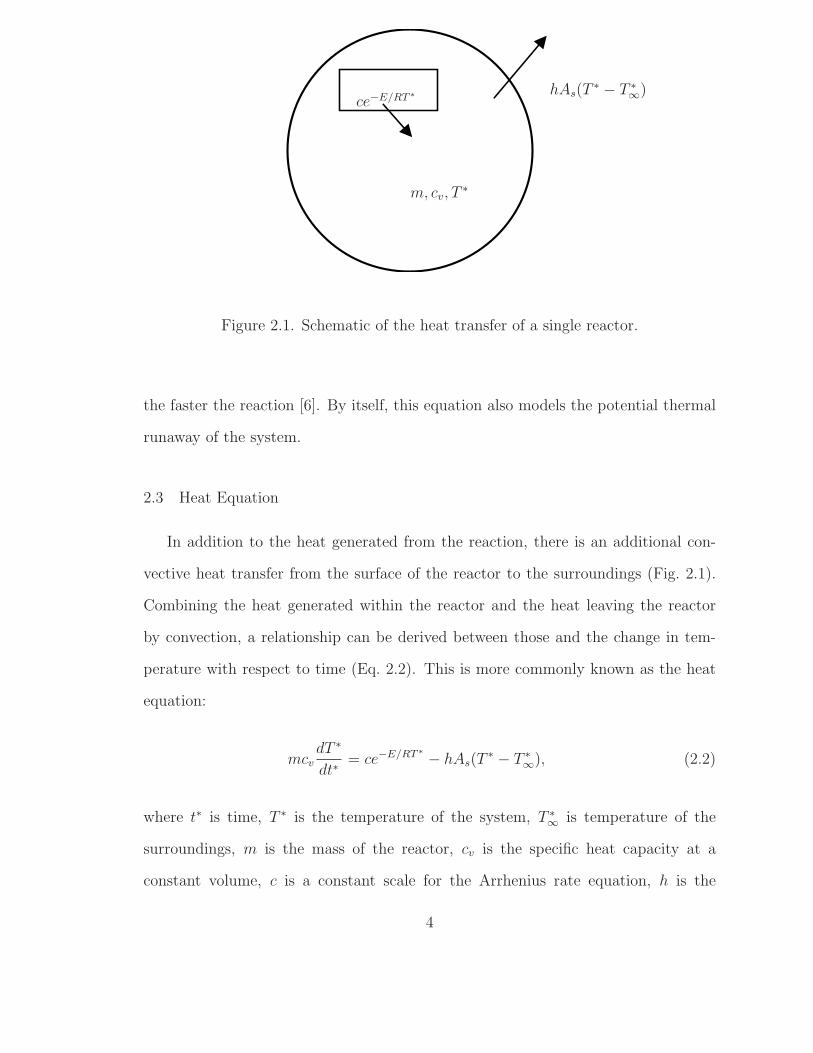
Figure 2.1. Schematic of the heat transfer of a single reactor.

the faster the reaction [6]. By itself, this equation also models the potential thermal

runaway of the system.

2.3 Heat Equation

In addition to the heat generated from the reaction, there is an additional con-

vective heat transfer from the surface of the reactor to the surroundings (Fig. 2.1).

Combining the heat generated within the reactor and the heat leaving the reactor

by convection, a relationship can be derived between those and the change in tem-

perature with respect to time (Eq. 2.2). This is more commonly known as the heat

equation:

mcvdT ∗

dt∗= ce−E/RT ∗ − hAs(T

∗ − T ∗

∞), (2.2)

where t∗ is time, T ∗ is the temperature of the system, T ∗

∞is temperature of the

surroundings, m is the mass of the reactor, cv is the specific heat capacity at a

constant volume, c is a constant scale for the Arrhenius rate equation, h is the

4

convection coefficient, and As is the reactor surface area. For this particular equation,

all of these variables are dimensional.

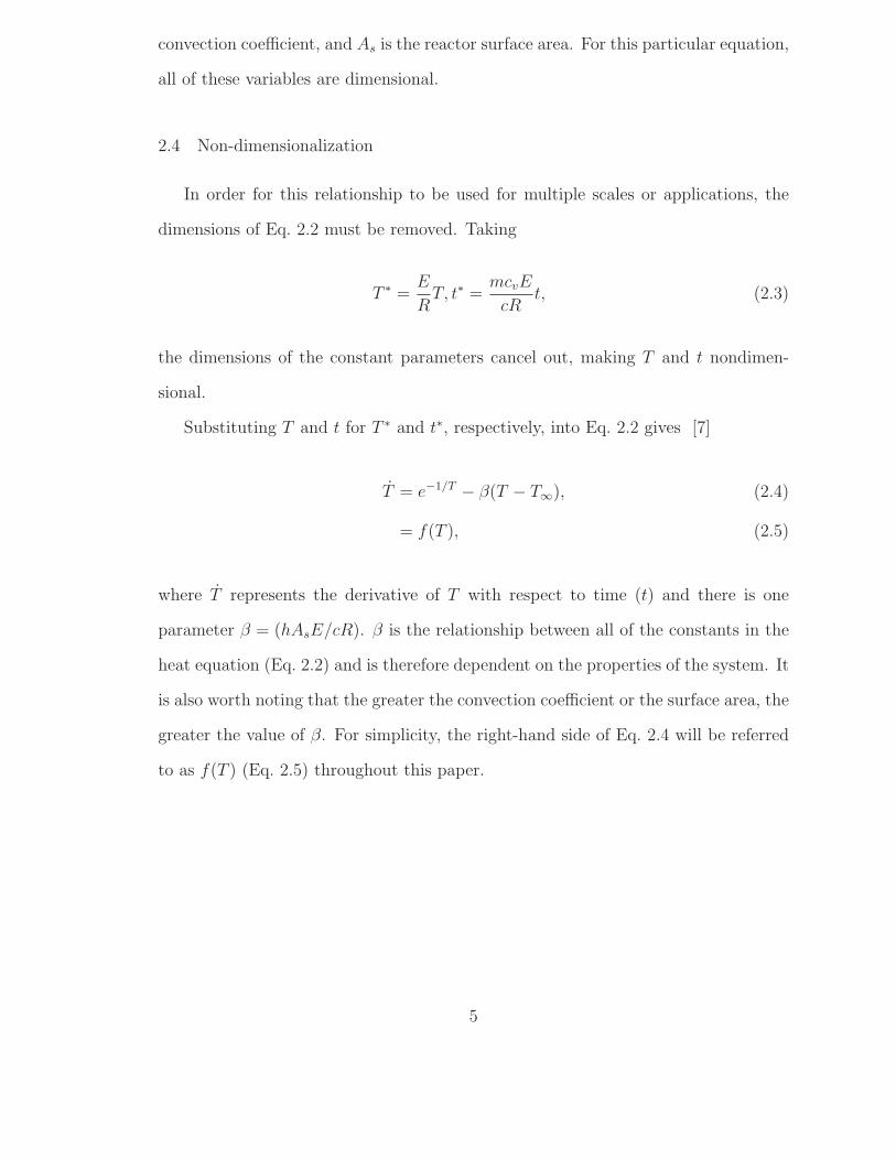
2.4 Non-dimensionalization

In order for this relationship to be used for multiple scales or applications, the

dimensions of Eq. 2.2 must be removed. Taking

T ∗ =E

RT, t∗ =

mcvE

cRt, (2.3)

the dimensions of the constant parameters cancel out, making T and t nondimen-

sional.

Substituting T and t for T ∗ and t∗, respectively, into Eq. 2.2 gives [7]

T = e−1/T − β(T − T∞), (2.4)

= f(T ), (2.5)

where T represents the derivative of T with respect to time (t) and there is one

parameter β = (hAsE/cR). β is the relationship between all of the constants in the

heat equation (Eq. 2.2) and is therefore dependent on the properties of the system. It

is also worth noting that the greater the convection coefficient or the surface area, the

greater the value of β. For simplicity, the right-hand side of Eq. 2.4 will be referred

to as f(T ) (Eq. 2.5) throughout this paper.

5

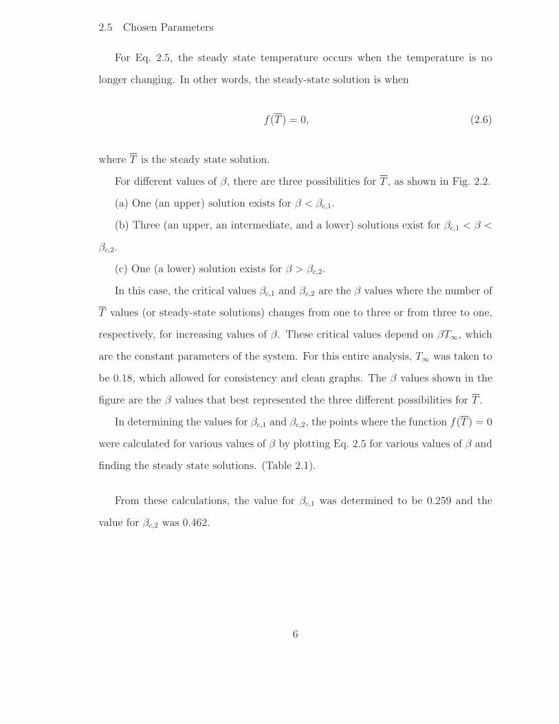
2.5 Chosen Parameters

For Eq. 2.5, the steady state temperature occurs when the temperature is no

longer changing. In other words, the steady-state solution is when

f(T ) = 0, (2.6)

where T is the steady state solution.

For different values of β, there are three possibilities for T , as shown in Fig. 2.2.

(a) One (an upper) solution exists for β < βc,1.

(b) Three (an upper, an intermediate, and a lower) solutions exist for βc,1 < β <

βc,2.

(c) One (a lower) solution exists for β > βc,2.

In this case, the critical values βc,1 and βc,2 are the β values where the number of

T values (or steady-state solutions) changes from one to three or from three to one,

respectively, for increasing values of β. These critical values depend on βT∞, which

are the constant parameters of the system. For this entire analysis, T∞ was taken to

be 0.18, which allowed for consistency and clean graphs. The β values shown in the

figure are the β values that best represented the three different possibilities for T .

In determining the values for βc,1 and βc,2, the points where the function f(T ) = 0

were calculated for various values of β by plotting Eq. 2.5 for various values of β and

finding the steady state solutions. (Table 2.1).

From these calculations, the value for βc,1 was determined to be 0.259 and the

value for βc,2 was 0.462.

6

0 1 2 3 4 5−1

−0.5

0

0.5

1

β = 1

β = 0.4

β = 0.2

T

f(T

)

Figure 2.2. f(T ) with T∞ = 0.18 and different βs

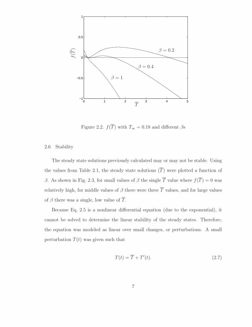
2.6 Stability

The steady state solutions previously calculated may or may not be stable. Using

the values from Table 2.1, the steady state solutions (T ) were plotted a function of

β. As shown in Fig. 2.3, for small values of β the single T value where f(T ) = 0 was

relatively high, for middle values of β there were three T values, and for large values

of β there was a single, low value of T .

Because Eq. 2.5 is a nonlinear differential equation (due to the exponential), it

cannot be solved to determine the linear stability of the steady states. Therefore,

the equation was modeled as linear over small changes, or perturbations. A small

perturbation T (t) was given such that

T (t) = T + T ′(t). (2.7)

7

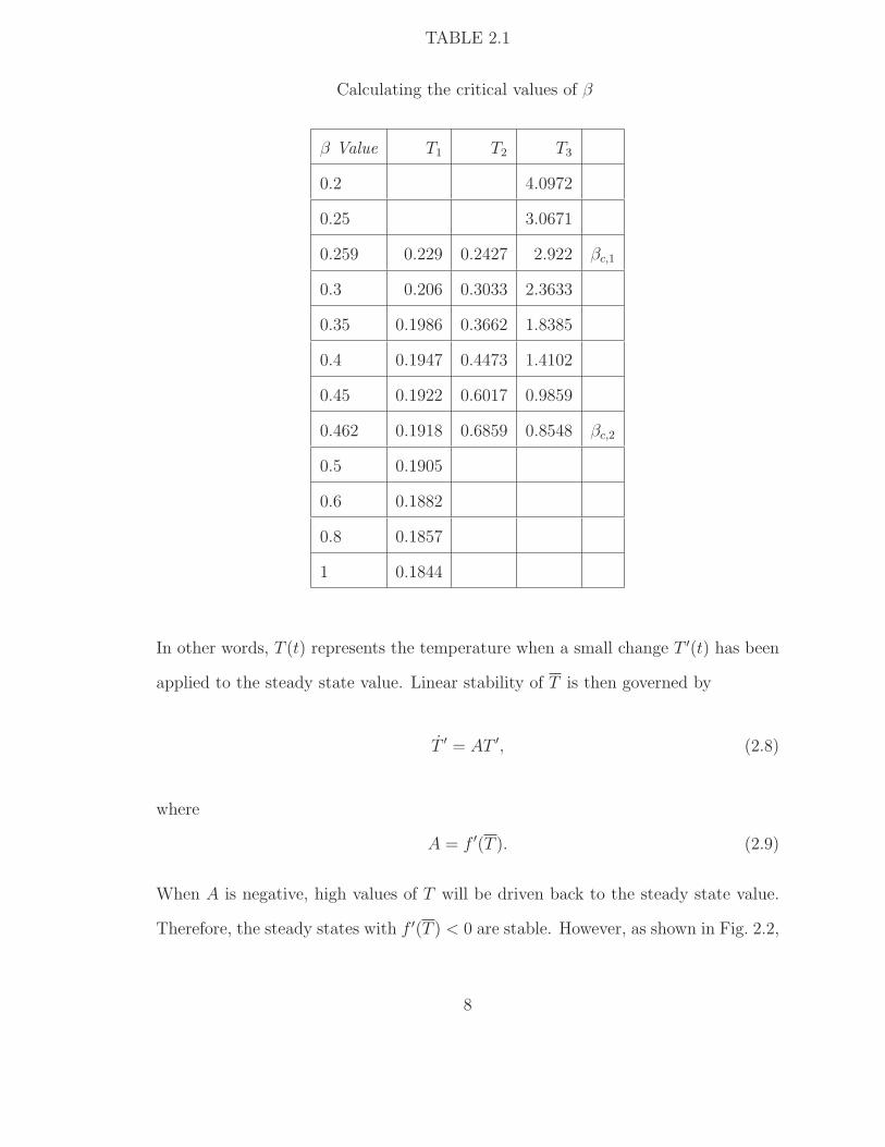
TABLE 2.1

Calculating the critical values of β

β Value T1 T2 T3

0.2 4.0972

0.25 3.0671

0.259 0.229 0.2427 2.922 βc,1

0.3 0.206 0.3033 2.3633

0.35 0.1986 0.3662 1.8385

0.4 0.1947 0.4473 1.4102

0.45 0.1922 0.6017 0.9859

0.462 0.1918 0.6859 0.8548 βc,2

0.5 0.1905

0.6 0.1882

0.8 0.1857

1 0.1844

In other words, T (t) represents the temperature when a small change T ′(t) has been

applied to the steady state value. Linear stability of T is then governed by

T ′ = AT ′, (2.8)

where

A = f ′(T ). (2.9)

When A is negative, high values of T will be driven back to the steady state value.

Therefore, the steady states with f ′(T ) < 0 are stable. However, as shown in Fig. 2.2,

8

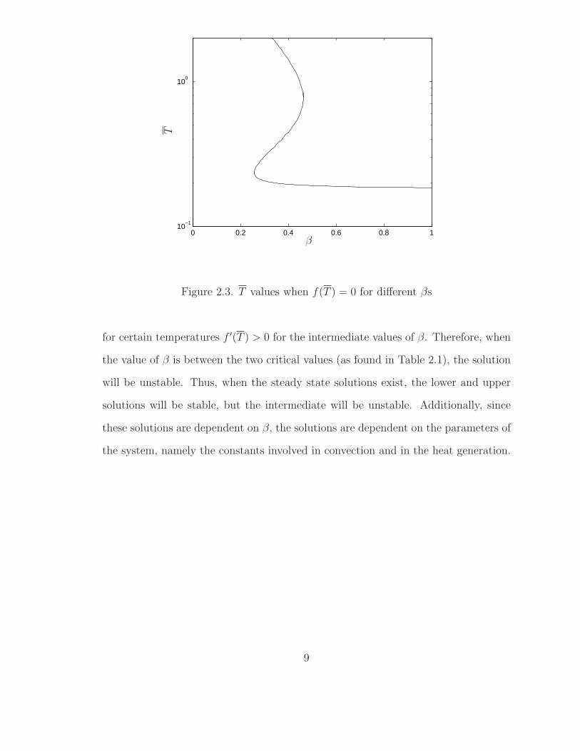
0 0.2 0.4 0.6 0.8 110

−1

100

T

β

Figure 2.3. T values when f(T ) = 0 for different βs

for certain temperatures f ′(T ) > 0 for the intermediate values of β. Therefore, when

the value of β is between the two critical values (as found in Table 2.1), the solution

will be unstable. Thus, when the steady state solutions exist, the lower and upper

solutions will be stable, but the intermediate will be unstable. Additionally, since

these solutions are dependent on β, the solutions are dependent on the parameters of

the system, namely the constants involved in convection and in the heat generation.

9

CHAPTER 3

COUPLED REACTORS

3.1 Motivation

The stability of the single reactor has been analyzed. A single reactor can have a

period of instability dependending on the properties and parameters of the system.

The single reactor in this analysis, however, is only dependent on the internal chemical

reaction and the convection to the surroundings. When the reactors are coupled,

there is an additional component of conduction between the reactors. The following

analysis examines how the conduction could affect stability.

3.2 Governing Equations

Just as with the single reactor, there is a component of internal heat generation.

Again, this is modeled using the Arrhenius rate equation

k ≈ e−E/RTi , (3.1)

where Ti is the temperature of the reactor in question. This is exactly the same as for a

single reactor. Likewise, there is also a component of convection to the surroundings.

Using the same analysis as for a single reactor (i.e. non-dimensionalization of the

heat equations), this relationship is found:

Ti = e−1/Ti − β(Ti − T∞) (3.2)

= f(Ti). (3.3)

10

Again, Ti is the temperature of the reactor in question. This relationship is exactly

the same as the one for the single reactor.

However, there will also be a conduction component between the reactors. Since

the reactors are arranged in a ring to neglect the end conditions, the conduction will

occur between the reactor in question and the reactors on either side. Combining the

conduction between the reactors with the heat transfer from the single reactor gives

this heat equation:

Ti = f(Ti) + K (Ti−1 − 2Ti + Ti+1) , (3.4)

where K represents the conduction coefficient between each reactor (and therefore

K > 0), i represents the reactor in question, and the parameter β is assumed to be

the same for all of the reactors.

3.3 Stability

Similar to the single reactor, steady state solutions satisfy

f(T i) + K(

T i−1 − 2T i + T i+1

)

= 0, (3.5)

or when the temperature of the reactor is no longer changing.

Because of the exponential function, Eq. 3.5 is a transcendental equation, and

therefore does not always have a finite set of roots. Transcendental equations can

have no roots, a finite set of roots, or an infinite set of roots. These roots can either

be real or complex. This analysis only investigated real roots because the complex

roots would add a component of oscillation that was beyond the scope of this study.

The system was studied for the possibilities of a single root (i.e. all reactors are the

same temperature) and two roots (i.e. alternating the reactor temperatures around

11

the ring).

3.3.1 Single Root

Having a single root for Eq. 3.5 can be written as T i = T where f(T ) = 0. The

linear stability of this is governed by

T′ = AT

′, (3.6)

where T′ is a vector of perturbations for each reactor

T′ =

T ′

1

T ′

2

...

T ′

n

, (3.7)

and A is a circulant matrix of the form

A =

f ′(T ) − 2K K . . . 0 K

K f ′(T ) − 2K K . . . 0

...

K 0 . . . K f ′(T ) − 2K

. (3.8)

Circulant matrices are matrices where the terms seem to rotate around each other.

For example, the 4x4 matrix

M =

c0 c3 c2 c1

c1 c0 c3 c2

c2 c1 c0 c3

c3 c2 c1 c0

(3.9)

12

is circulant because each term moves a place to the right and the rightmost terms

move to the leftmost position as they go down the rows. Eigenvalues for an nxn

circulant matrix are given by

λj = c0 + c1ωj + c2ω2j + c3ω

3j + · · · + cn−1ω

n−1j , (3.10)

where

ωj = e(2πij/n), (3.11)

and j = 0 . . .n-1 and i =√−1. The value of ωj will travel along the unit circle,

therefore causing the eigenvalues to oscillate between -1 and 1 [8].

Therefore, the n eigenvalues of the symmetric, circulant matrix A from Eq. 3.8

are [9]

λj = f ′(T ) − K(

2 − e2πji/n − e2πji(n−1)/n)

(3.12a)

= f ′(T ) − 2K

(

1 − cos2πj

n

)

, (3.12b)

for j = 0, 1, . . . , n − 1. If all λj < 0, then the system will be stable. Since f ′(T )

can be positive or negative depending on β, Eq. 3.12b will need to be evaluated for

both situations. Each solution reacts differently: (i) If f ′(T ) < 0, i.e. for the lower

and upper solutions, the previously stable solutions continue to be stable. This is

because K is always greater than 0, and the term next to it can never be negative

because cosine oscillates between -1 and 1. Therefore, if the f ′(T ) term is negative,

the K term will always be subtracted from it, therefore making the eigenvalues more

negative. Thus, the system remains stable. (ii) If f ′(T ) > 0, i.e. for the intermediate

13

solution, the previously unstable solution may seemingly be stable if

K >f ′(T )

2 (1 − cos 2πj/n), (3.13)

for all j = 0, 1, . . . , n. However, when j = 0, the denominator becomes 0 and

therefore the minimum required value of K approaches infinity. If λ0 > 0, not all λj

are negative, and therefore the system will be unstable. Therefore, for a single root

(or fixed point) of Eq. 3.5, the systems that cause a single reactor to be stable will

continue to be stable and the systems that cause a single reactor to be unstable will

continue to be unstable.

3.3.2 Two Roots

Another solution to Eq. 3.5 that was studied was the possibility that every other

reactor would have the same temperature. In other words, the even reactors would

have one temperature and the odd reactors would have another temperature. The

methodology used was the same as the single root, and the equations were solved

numerically. The results are in the next section.

14

CHAPTER 4

NUMERICAL RESULTS

4.1 Motivation

To understand how the temperature of the reactors changes over time, the nu-

merical solutions to Eq. 2.4 and Eq. 3.4 were calculated using Newton’s Method. For

each plot, the steady state solutions are plotted as dashed lines.

4.2 Single Reactor

For a single reactor, the approximate solution for Eq. 2.4 was calculated and

plotted for different initial values of T , as shown in the following figures.

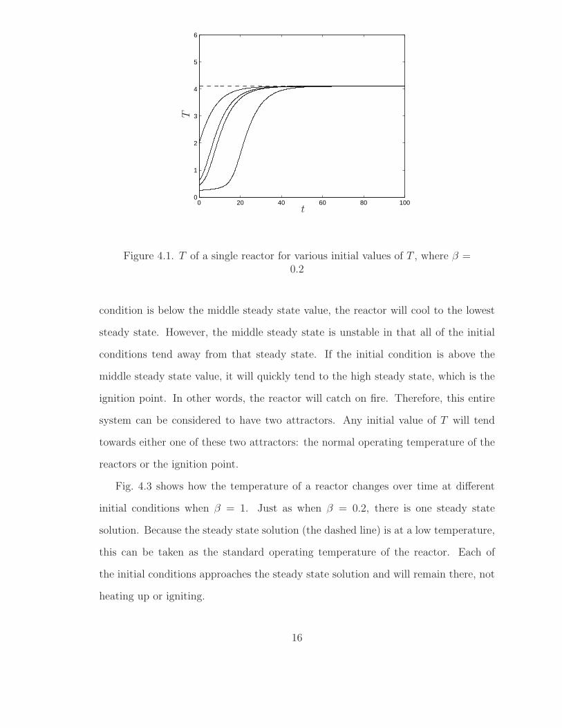
Fig. 4.1 shows how the temperature of the reactor changes over time from various

initial conditions when β = 0.2. The steady state solution (the dashed line), because

it is at a high temperature, can be interpreted as the ignition point . No matter what

the initial condition of the reactor is, it will eventually reach the steady state and

simply burn. Because each of the initial conditions approaches the steady solution,

this is stable.

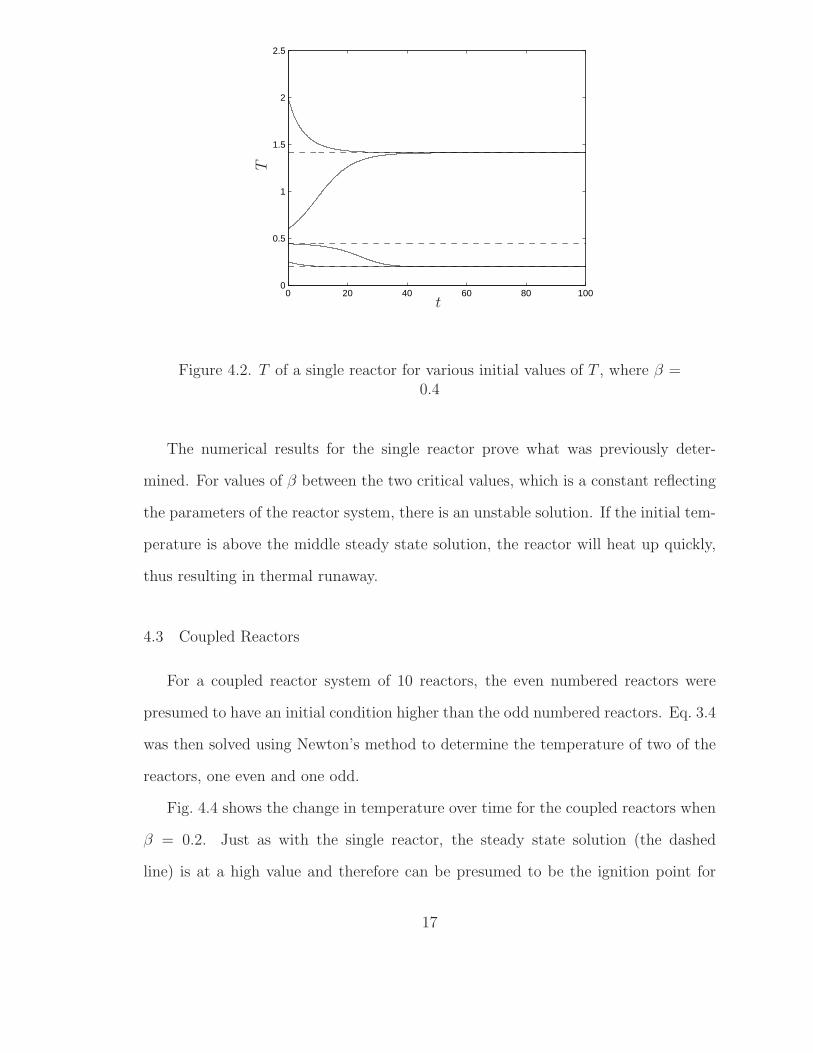
Fig. 4.2 shows how various initial conditions for the temperature change over time

when β = 0.4. There are three steady-state solutions- the top dashed line can be

considered the ignition point (i.e. when the reactor catches on fire). If the reactor

starts at a temperature higher than this steady state, it will eventually cool down

to the steady state temperature while still burning. The bottom steady state can

be considered the normal running temperature of the reactor. As long as the initial

15

0 20 40 60 80 1000

1

2

3

4

5

6

T

t

Figure 4.1. T of a single reactor for various initial values of T , where β =0.2

condition is below the middle steady state value, the reactor will cool to the lowest

steady state. However, the middle steady state is unstable in that all of the initial

conditions tend away from that steady state. If the initial condition is above the

middle steady state value, it will quickly tend to the high steady state, which is the

ignition point. In other words, the reactor will catch on fire. Therefore, this entire

system can be considered to have two attractors. Any initial value of T will tend

towards either one of these two attractors: the normal operating temperature of the

reactors or the ignition point.

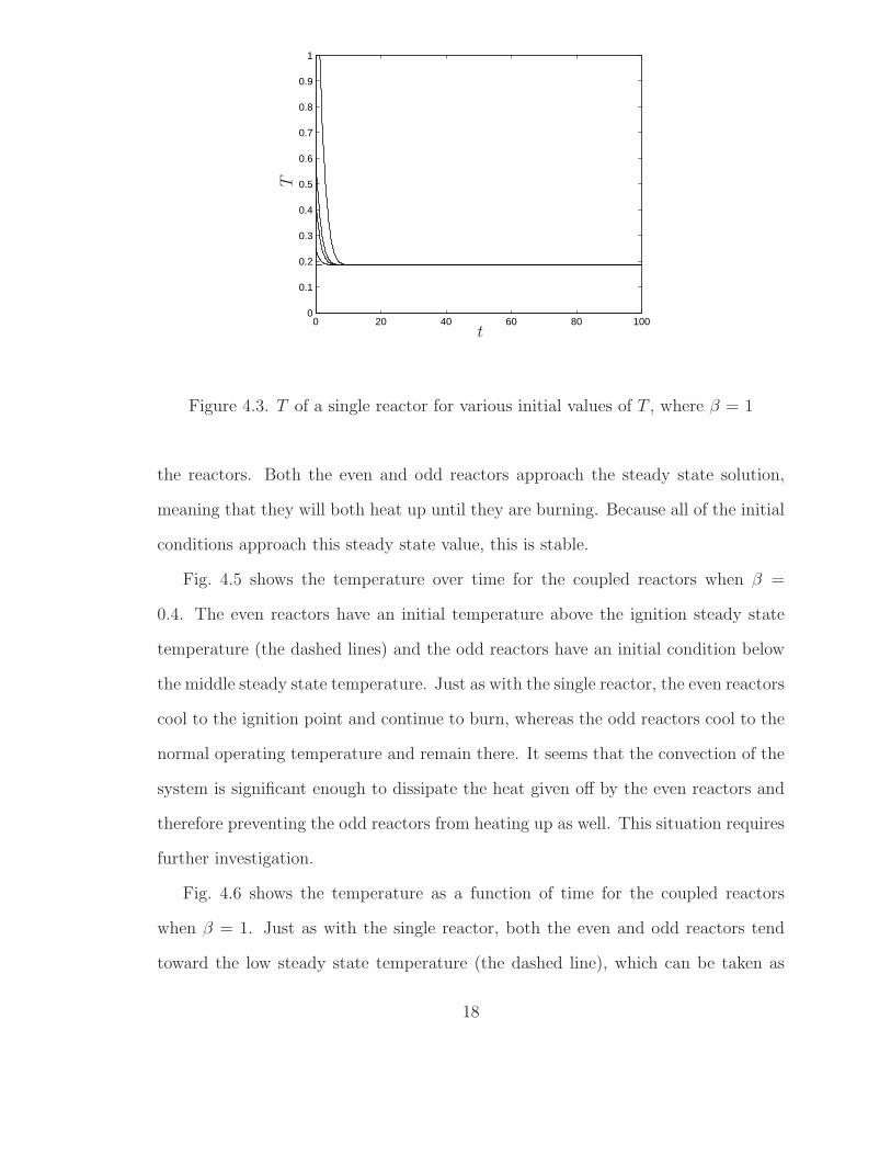
Fig. 4.3 shows how the temperature of a reactor changes over time at different

initial conditions when β = 1. Just as when β = 0.2, there is one steady state

solution. Because the steady state solution (the dashed line) is at a low temperature,

this can be taken as the standard operating temperature of the reactor. Each of

the initial conditions approaches the steady state solution and will remain there, not

heating up or igniting.

16

0 20 40 60 80 1000

0.5

1

1.5

2

2.5

T

t

Figure 4.2. T of a single reactor for various initial values of T , where β =0.4

The numerical results for the single reactor prove what was previously deter-

mined. For values of β between the two critical values, which is a constant reflecting

the parameters of the reactor system, there is an unstable solution. If the initial tem-

perature is above the middle steady state solution, the reactor will heat up quickly,

thus resulting in thermal runaway.

4.3 Coupled Reactors

For a coupled reactor system of 10 reactors, the even numbered reactors were

presumed to have an initial condition higher than the odd numbered reactors. Eq. 3.4

was then solved using Newton’s method to determine the temperature of two of the

reactors, one even and one odd.

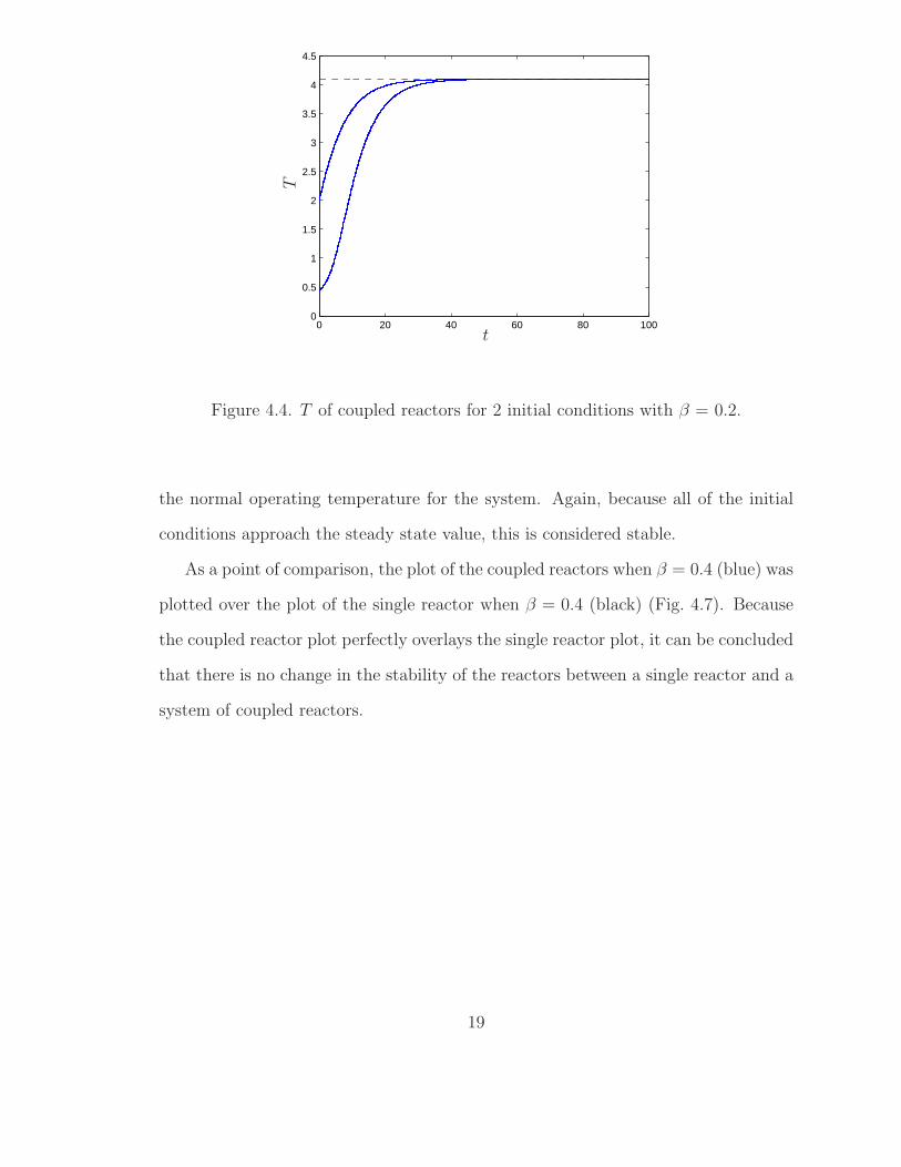
Fig. 4.4 shows the change in temperature over time for the coupled reactors when

β = 0.2. Just as with the single reactor, the steady state solution (the dashed

line) is at a high value and therefore can be presumed to be the ignition point for

17

0 20 40 60 80 1000

0.1

0.2

0.3

0.4

0.5

0.6

0.7

0.8

0.9

1

T

t

Figure 4.3. T of a single reactor for various initial values of T , where β = 1

the reactors. Both the even and odd reactors approach the steady state solution,

meaning that they will both heat up until they are burning. Because all of the initial

conditions approach this steady state value, this is stable.

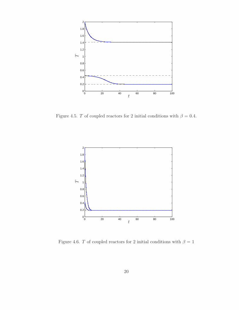
Fig. 4.5 shows the temperature over time for the coupled reactors when β =

0.4. The even reactors have an initial temperature above the ignition steady state

temperature (the dashed lines) and the odd reactors have an initial condition below

the middle steady state temperature. Just as with the single reactor, the even reactors

cool to the ignition point and continue to burn, whereas the odd reactors cool to the

normal operating temperature and remain there. It seems that the convection of the

system is significant enough to dissipate the heat given off by the even reactors and

therefore preventing the odd reactors from heating up as well. This situation requires

further investigation.

Fig. 4.6 shows the temperature as a function of time for the coupled reactors

when β = 1. Just as with the single reactor, both the even and odd reactors tend

toward the low steady state temperature (the dashed line), which can be taken as

18

0 20 40 60 80 1000

0.5

1

1.5

2

2.5

3

3.5

4

4.5

T

t

Figure 4.4. T of coupled reactors for 2 initial conditions with β = 0.2.

the normal operating temperature for the system. Again, because all of the initial

conditions approach the steady state value, this is considered stable.

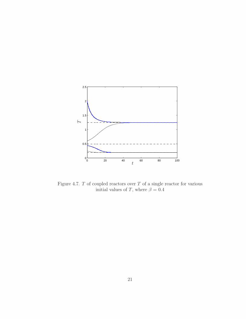
As a point of comparison, the plot of the coupled reactors when β = 0.4 (blue) was

plotted over the plot of the single reactor when β = 0.4 (black) (Fig. 4.7). Because

the coupled reactor plot perfectly overlays the single reactor plot, it can be concluded

that there is no change in the stability of the reactors between a single reactor and a

system of coupled reactors.

19

0 20 40 60 80 1000

0.2

0.4

0.6

0.8

1

1.2

1.4

1.6

1.8

2

T

t

Figure 4.5. T of coupled reactors for 2 initial conditions with β = 0.4.

0 20 40 60 80 1000

0.2

0.4

0.6

0.8

1

1.2

1.4

1.6

1.8

2

T

t

Figure 4.6. T of coupled reactors for 2 initial conditions with β = 1

20

0 20 40 60 80 1000

0.5

1

1.5

2

2.5

T

t

Figure 4.7. T of coupled reactors over T of a single reactor for variousinitial values of T , where β = 0.4

21

CHAPTER 5

CONCLUSIONS AND RECOMMENDATIONS

5.1 Summary

This paper investigated the potential instability of coupled reactors in order to

determine whether or not placing the reactors in close proximity to each other makes

the system more or less stable. The system was analyzed in a ring so as to neglect

the unknown end conditions. First, the stability of a single reactor was investigated

by analyzing the heat transfer involved. It was discovered that depending on the

parameters of the system, there were three potential solutions: a stable solution where

the reactors approached at a low operating temperature, an unstable solution where

the reactors would quickly ignite, and a third where the reactors would approach a

steady high temperature, where the reactors could be considered to have ignited.

This analysis was then applied to the coupled reactor system. Each individual

reactor had the same heat transfer as the single reactor system, but with an additional

component of conduction between the reactors. Two situations were examined, one

where the temperature of each reactor was at the steady state temperature (i.e. where

the temperature was no longer changing), and one where the initial temperature of the

even numbered reactors was higher than the initial temperature of the odd numbered

reactors. It was found that the situations where a single reactor would be unstable

were also the situations where coupled reactors would be unstable, and likewise when

the single reactor would be stable, the coupled reactors would be stable. Therefore,

it was concluded that coupling the reactors did not affect the stability of the reactors,

at least for those two situations.

22

5.2 Applications

The analysis performed can be used in industry to determine whether or not to

use single or coupled reactors and how the stability of the system will be affected. As

mentioned above, it was determined that whether or not the reactors are coupled has

very little to do with the stability of the system. The stability has far more depen-

dence on the parameters of the system than whether or not the reactors are coupled.

The primary parameter in the analysis was the relationship between the convection

and the heat generation constants involved in the heat transfer of the reactor. As

mentioned before, the stable solutions were those where the reactor was either ap-

proaching a low operating temperature or approaching a high ignition temperature.

For most industrial applications, fire tends to be avoided and therefore the system

that approaches a low operating temperature would be best. This solution correlates

to the convection constants being greater than the heat generation constants. To

prevent a system becoming unstable, therefore, one can increase the surface area of

the system or adjust the convection coefficient by adding a fan or a fluid to increase

the heat transferred through convection. This way, whether the reactors are single

or coupled, they should remain stable.

5.3 Limitations and Recommendations

This analysis still depends on several assumptions. First, the coupled reactors

were placed in a ring to neglect the end conditions. In industrial settings, placing

the reactors in a ring may not be possible, and therefore the end conditions could

affect the behavior of the reactors. Because this analysis focused on the interaction

between the reactors, the end conditions could be ignored. Additional studies could

look into the possible effects of including end conditions.

Additionally, the chemical reaction within the reactors was modeled using a con-

23

stant before the Arrhenius rate equation. As the reaction proceeds within the reactor,

the proportion of reacted molecules to unreacted molecules will change, which could

have an effect on the significance of the chemical reaction. In other words, as the fuel,

so to speak, is used, there will be less fuel to proceed with the rest of the reaction,

which could therefore change the influence of the Arrhenius equation (i.e. change

the constant in front of the equation). This could affect the stability of the reactors

when the system is analyzed for a long period of time. Further studies could look

into the effects of this phenomenon.

Lastly, in the analysis of the coupled reactors, only two situations were examined.

Due to the nature of the equations, there could be infinitely many solutions that differ

from the analysis performed here. In order to get a better understanding, further

research could investigate other situations, such as each reactor being a different

temperature. Additionally, in the analysis the dual root equation used the same

equations as the situation when the temperature of the reactor was the steady state

temperature. This may not be the best analysis. Further studies could look into

different methods of solving such a system.

24

BIBLIOGRAPHY

1. M.R. Rahimpour, M.H. Khademi, and A.M. Bahmanpour. A comparison of con-ventional and optimized thermally coupled reactors for fischertropsch synthesis in{GTL} technology. Chemical Engineering Science, 65(23), 2010.

2. F. Torabi and V. Esfahanian. Study of thermal-runaway in batteries. Journal of

The Electrochemical Society, 160(2), 2012.

3. Claus G. Zimmermann. Thermal runaway in multijunction solar cells. Applied

Physics Letters, 102(23), 2013.

4. Qingsong Wang, Ping Ping, Xuejuan Zhao, Guanquan Chu, Jinhua Sun, andChunhua Chen. Thermal runaway caused fire and explosion of lithium ion battery.Journal of Power Sources, 208(0), 2012.

5. J. O’Brien. Behavior Prediction and Control of Thermostatically-Controlled,

Thermally-Coupled, Self-Excited Oscillators. 2012.

6. Guenevieve Del Mundo, Kareem Moussa, Pamela Chacha, Florence-Damilola Od-ufalu, Galaxy Mudda, Kan, and Chin Fung Kelvin. Arrhenius equation. UC Davis

Chem Wiki.

7. J.D. Buckmaster and G.S.S. Ludford. Lectures on Mathematical Combustion.SIAM, Philadelphia, PA, 1983.

8. P.J. Davis. Circulant Matrices. John Wiley, New York, 1979.

9. R. Aldrovandi. Special Matrices of Mathematical Physics: Stochastic, Circulant,

and Bell Matrices. World Scientific, River Edge, NJ, 2001.

This document was prepared & typeset with LATEX2ε, and formatted withnddiss2ε classfile (v3.2013[2013/04/16]) provided by Sameer Vijay and updated

by Megan Patnott.

25