epl draft

Stability in Chaos

Greg Huber1, Marc Pradas2,1, Alain Pumir3,1 and Michael Wilkinson2,1

1 Kavli Institute for Theoretical Physics, University of California Santa Barbara, CA93106, USA3 Department of Mathematics and Statistics, The Open University, Walton Hall, Milton Keynes, MK7 6AA, UK3 Laboratoire de Physique, Ecole Normale Superieure de Lyon, CNRS, Universite de Lyon, F-69007, Lyon, France

PACS 05.10.Gg – Stochastic analysis methods (Fokker-Planck, Langevin, etc.)PACS 05.45.-a – Nonlinear Dynamics and ChaosPACS 05.40.-a – Fluctuation phenomena, random processes, noise, and Brownian motion

Abstract – Intrinsic instability of trajectories characterizes chaotic dynamical systems. We reporthere that trajectories can exhibit a surprisingly high degree of stability, over a very long time,in a chaotic dynamical system. We provide a detailed quantitative description of this effect fora one-dimensional model of inertial particles in a turbulent flow using large-deviation theory.Specifically, the determination of the entropy function for the distribution of finite-time Lyapunovexponents reduces to the analysis of a Schrodinger equation, which is tackled by semi-classicalmethods.

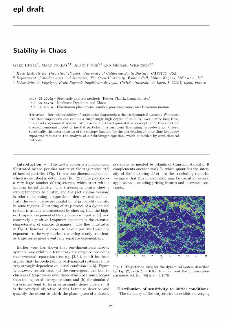
Introduction. – This Letter concerns a phenomenonillustrated by the peculiar nature of the trajectories x(t)of inertial particles (Fig. 1) in a one-dimensional model,which is described in detail later (Eq. (2)). The plot showsa very large number of trajectories, which start with auniform initial density. The trajectories clearly show astrong tendency to cluster, and the plot (online version)is color-coded using a logarithmic density scale to illus-trate the very intense accumulation of probability densityin some regions. Clustering of trajectories of a dynamicalsystem is usually characterised by showing that the high-est Lyapunov exponent of the dynamics is negative [1], andconversely a positive Lyapunov exponent is the essentialcharacteristic of chaotic dynamics. The flow illustratedin Fig. 1, however, is known to have a positive Lyapunovexponent, so the very marked clustering is only transient,as trajectories must eventually separate exponentially.

Earlier work has shown that one-dimensional chaoticsystems may exhibit a temporary convergence precedingtheir eventual separation (see, e.g. [2, 3]), and it has beenargued that the predictability of dynamical systems can bevery strongly dependent on initial conditions [4,5]. Figure1, however, reveals that: (a) the convergence can lead toclusters of trajectories over times which are much longerthan the expected divergence time, and (b) the simulatedtrajectories tend to form surprisingly dense clusters. Itis the principal objective of this Letter to describe andquantify the extent to which the phase space of a chaotic

system is permeated by islands of transient stability. Itcomplements another work [6] which quantifies the inten-sity of the clustering effect. In the concluding remarks,we argue that this phenomenon may be useful for severalapplications, including pricing futures and insurance con-tracts.

Fig. 1: Trajectories, x(t), for the dynamical system describedby Eq. (2) with ξ = 0.08, L = 2π, and the dimensionlessparameter [cf. Eq. (9)] is ε = 1.7678.

Distribution of sensitivity to initial conditions.– The tendency of the trajectories to exhibit converging

p-1

Greg Huber1, Marc Pradas2,1, Alain Pumir3,1 and Michael Wilkinson2,1

−0.5 −0.25 0 0.25 0.50

0.2

0.4

0.6

0.8

1

z/γ

Π (

z/γ)

ε = 1.768

γT=2.56γT=5.12γT=10.24γT=20.48γT=40.96

Fig. 2: Cumulative probability, Π, for the value of the FTLE,z(t), at different times (in dimensionless units). The distri-bution of z(t) is very broad, even for large values of t. Theparameters are the same as for Fig. 1.

behavior is illustrated in Fig. 2, which shows the cumula-tive probability, Π, for the finite-time Lyapunov exponent(FTLE) at long times. The FTLE at time t for a trajec-tory starting at x0 is defined by

z(t) =1

tln

∣∣∣∣ ∂xt∂x0

∣∣∣∣x(0)=x0

, (1)

where xt denotes position at time t. The expectation valueof z(t) in the limit as t→∞ is termed the Lyapunov ex-ponent: Λ = limt→∞〈z(t)〉 (angular brackets denote en-semble averages throughout). When Λ > 0, there is analmost certain exponential growth of infinitesimal separa-tions of trajectories. For the example in Fig. 1, we haveΛ = 0.075 γ, where γ is a positive parameter of the model[cf. Eq. (2)]. Figure 2 shows that the cumulative probabil-ity distribution for z is very broad: even at time t = 41/γ,which is comparable to the duration of the trajectoriesshown in Fig. 1, the probability of z being negative is ashigh as 0.25. We shall see how this very broad distributioncan be quantified.

It is usually assumed that when the highest Lyapunovexponent is positive, the long-term behavior of a systemis inherently unpredictable because of exponential sensi-tivity to the initial conditions. However, the phenomenonillustrated in Figs. 1 and 2 indicates that there may bebasins in the space of initial conditions which attract asignificant fraction of the phase space, giving a final po-sition which is highly insensitive to the initial conditions.If the initial conditions which are of physical interest liewithin one of these basins, the behavior of the system canbe computed accurately for a time which is many multiplesof the inverse of the Lyapunov coefficient.

Next we describe the equations of motion which wereused to generate Fig. 1. They correspond to

x = v,

−1.5 −1 −0.5 0 0.5 1 1.5−0.5

0

0.5

1

1.5

2

2.5

z/γ

−ln

[ P

(z/γ

) ]/

(γ T

)

ε = 1.768

γT=5.12

γT=10.24

γT=20.48

γT=40.96

Fig. 3: The transformed probability density function− ln P (z)/t approaches a limit, termed the large deviation en-tropy function J(z). When t→∞, we find excellent agreementwith a theoretical prediction for J(z) (dashed line).

v = γ[u(x, t)− v], (2)

where x and v are the position and velocity, respectively,of a small particle in a viscous fluid [7, 8]; γ is a constantdescribing the rate of damping of the motion of a smallparticle relative to the fluid and u(x, t) is a randomly fluc-tuating velocity field of the fluid in which the particles aresuspended. In Fig. 1 we simulated a velocity field wherethe correlation function is white noise in time, satisfying〈u(x, t)〉 = 0 and 〈u(x, t)u(x′, t′)〉 = δ(t−t′)C(x−x′). Thecorrelation function is C(∆x) = Dξ2 exp

(−∆x2/2ξ2

),

where D and ξ are constants. Trajectories which leavethe interval [0, L] are returned there by adding a multipleof L to x.

Large-deviation analysis. – In the large-time limitthe probability density of z is expected to be described bya large deviation approximation [9, 10]:

P (z) ∼ exp[−tJ(z)], (3)

where J(z) is termed the entropy function or the rate func-tion. We are able to explain the broad distribution illus-trated in Fig. 2 by determining the entropy function J(z):if the second derivative, J ′′(Λ), is small, the FTLE hasa very broad distribution, giving a quantitative explana-tion for Fig. 2. In Fig. 3 we compare the entropy functionobtained from our empirical distribution of z with a theo-retical curve (described below). There is very satisfactoryagreement as t→∞, indicating that the effect illustratedin Figs. 1 and 2 has been understood quantitatively.

Our theoretical approach involves the analysis of a cu-mulant, λ(k), which is defined by

〈exp(kzt)〉 = exp [tλ(k)] . (4)

The large deviation principle, as represented by equation

p-2

Stability in Chaos

(3), implies that

〈exp(kzt)〉 =

∫ ∞−∞

dz exp[t(kz − J(z))]. (5)

A Laplace estimate shows that λ and J are a Legendretransform pair:

λ(k) = kz − J(z), J ′(z) = k. (6)

For the model described by Eq. (2), the cumulant canbe determined as an eigenvalue of a differential equation.Following the approach discussed in [11], we can obtain aFokker-Planck equation for the variables Y and Z definedby Z = δx

δx and Z = Y :

∂ρ

∂t= −∂Y (Zρ) + Fρ, (7)

where we have defined Fρ ≡ ∂Z(v(Z)ρ) + Dγ2∂2Zρ withv(Z) = −γZ − Z2. Note that Y = zt, and we introducethe Lyapunov exponent, Λ = 〈Z〉. The cumulant λ(k) isthe largest eigenvalue of the operator F + kZ [12]:

Fρ(Z) + kZρ(Z) = λ(k)ρ(Z) . (8)

It is convenient to make a transformation of coordinates:

x = (γD)−1/2

Z , ε =

√Dγ, E = −λ

γ. (9)

The parameter ε is a dimensionless measure of the strengthof inertial effects in the model (2). It is known that theLyapunov exponent Λ is negative, indicating almost cer-tain coalescence of paths, when ε < εc = 1.3309 . . . [13].For ε > εc, the Lyapunov exponent is positive so that themotion is chaotic. All of the illustrations in this paperare at ε = 1.7678 ≈ 1.33 . . . × εc, where Λ ≈ 0.075 γ.In the coordinates defined by (9), the cumulant obeys anequation of the form

∂x(∂x + x+ εx2)ρ(x) + kεxρ(x) + Eρ(x) = 0 . (10)

Bohr-Sommerfeld quantisation for cumulants. –We now transform (10) so that it takes the form of a

Schrodinger equation. Write F = ∂x[∂x+x+εx2] and con-sider a gauge transformation H = exp[−Φ(x)]F exp[Φ(x)]with Φ(x) = −x2/4 − εx3/6. The cumulant λ(k) is thenobtained from the ground-state eigenvalue E0 of a Her-mitean operator

ψ′′ − V (x)ψ = Eψ (11)

where λ = −E0/γ and the potential is

V (x) =1

4(x+ εx2)2 − 1

2− ε(k + 1)x . (12)

Note that Eq. (11) corresponds to a Schrodinger equationwith m = 1

2 and h = 1. We remark that, when ε is small,

the potential V (x) has two minima, close to x = 0 and tox = −1/ε.

The WKB method [14, 15] provides a powerful toolfor understanding the structure of solutions of theSchrodinger equation. It works best when the potentialenergy is slowly varying. In the case of equation (11), ε isthe small parameter of WKB theory, because the minimaof the potential move apart as ε→ 0. In fact, a change ofvariable x = εX formally reduces Eq. (11) to an expressionwhere the ψ′′ term has a small coefficient. We will find,however, that WKB methods yield surprisingly accurateresults even when ε is not small. Define the momentum

p(x) = +√V (x)− E, (13)

with p(x) = 0 where V (x) < E. The action integral is

S(x) =

∫ x

0

dx′ p(x′), (14)

and define a pair of WKB functions

φ±(x) =1√p(x)

exp[±S(x)] . (15)

Then, as we get further away from turning points wherep(x) = 0, the solutions of (11) are asymptotic to a lin-ear combination of WKB solutions f(x) = a+φ+(x) +a−φ−(x), where a± are approximately constant, except inthe vicinity of turning points where E = V (x).

The Schrodinger equation (11) has unusual boundaryconditions. The gauge transformation implies that thesolutions of (10) and (11) are related by

ψ(x) = exp[−Φ(x)]ρ(x) = exp

[x2

4+ ε

x3

6

]ρ(x) . (16)

Integration of equation (10) gives∫ ∞−∞

dx (kεx+ E)ρ(x) = 0, (17)

so that 〈x〉 must be finite. Then equation (16) impliesthat the coefficient of a− must be zero as x→ −∞ (so thatρ(x) does not diverge). Furthermore, ρ(x) has an algebraicdecay as x → ±∞ and the coefficients of these algebraictails must be equal in order for 〈x〉 to be finite. In terms ofthe coefficients a±, the appropriate boundary conditionsare therefore limx→−∞ a+ = 1 and limx→−∞ a− = 0. Atlarge positive values of x, we have

limx→+∞

{a+ = exp(Σ)a− = c

(18)

where c is indeterminate, and where Σ is defined by thefinite limit of the following expression:

Σ = limx→∞

[S(x)− S(−x)− Φ(x) + Φ(−x)] . (19)

We can determine the smallest eigenvalue E(k) by usinga shooting method to find a solution which satisfies (18).

p-3

Greg Huber1, Marc Pradas2,1, Alain Pumir3,1 and Michael Wilkinson2,1

Solving numerically (11) amounts to propagating a two-dimensional vector a(x) = (ψ(x), ψ′(x)). We can takean initial condition for xi large and negative in the formai = (1, p(xi)) exp(Φ(xi)), corresponding to the asymp-totic form of the solution which decays as x → −∞. Wenumerically propagate this solution for increasing x, andfind that the solution increases exponentially. If the firstelement of the solution vector at xf � 1 is a1(xf) = ψ(xf),we can express the eigenvalue condition in the followingform:

f(k, ε, E) ≡ ψ(xf) exp[Φ(xf)]

ψ(xi) exp[Φ(xi)]= 1 . (20)

This shooting method does provide very accurate valuesfor the cumulant λ = −γE0.

It is also desirable to be able to make analytical esti-mates of the eigenvalues. The coefficients a± can be ap-proximated as changing discontinuously when x passes aturning point, where E − V (x) is zero (or close to zero).Depending on the value of E there may be one or twodouble turning points. We must take account of the factthat the amplitudes a± can change ‘discontinuously’ inthe vicinity of turning points. Close to a double turningpoint, the equation is approximated by a parabolic cylin-der equation

d2ψ

dx2− 1

4x2ψ + Eψ = 0. (21)

We are interested in constructing a solution which is ex-ponentially increasing as x increases, both when x→ −∞and for x → +∞. We can use this solution in the formφ(x) = A(x) exp[S(x)]/

√p(x) where A(x) is asymptoti-

cally constant as x → ±∞, and we take A(−∞) = 1. Byadapting a calculation due to Miller and Good [16], wefind that as x → +∞, the solution is approximated byA(x) = F (E), where he function F (E) is

F (E) =

√2π

Γ( 12 − E)

exp[E(1− ln |E|)], (22)

and has zeros at E = n+ 12 , n = 0, 1, 2, . . .. It approaches

unity as E → −∞ and it oscillates approximately sinu-soidally with amplitude equal to 2 as E → +∞. Equa-tion (22) can be used to determine the amplitude of theexponentially increasing solution after passing through adouble turning point.

The eigenvalue condition (20) can also be expressed us-ing the WKB approximation, leading to a generalisationof the Bohr-Sommerfeld quantisation condition. We con-sider cases where the potential has a closely spaced pairof real turning points, which will be treated as a doubleturning point, close to x = 0. The effect of the doubleturning point is to cause the WKB amplitude of the expo-nentially increasing solution φ+(x) to change by a factorF (E), which we assume to be given correctly by the ex-pression for a parabolic potential, Eq. (22). Because thepotential is not precisely parabolic at the double turning

-2.5

-2

-1.5

-1

-0.5

0

0.5

-2 -1 0 1 2

E(k

)

k

f=0, exactf=0, WKB

f=1, exactf=1, WKB

Fig. 4: The generalised Bohr-Sommerfeld quantisation condi-tion, Eq. (24), produces remarkably accurate eigenvalues. Theupper curves are eigenvalues with the usual boundary condition(square-integrable wavefunction), with f = 0, comparing thenumerically exact eigenvalue with that obtained by the Bohr-Sommerfeld condition. The lower curves are for the criterionf = 1 which applies to our cumulant eigenvalues. These dataare for the case ε = 1.7678, and the dashed line in Fig. 3 isthe Legendre transform of the numerically exact eigenvalue forf = 1.

point, the energy argument of F (E) should be replaced byF (σ/π), where σ is a phase integral:

σ =

∫ x2

x1

dx√E − V (x), (23)

with x1 and x2 being the turning points where E = V (x).This is the most natural choice of replacement variable,because it reproduces the standard Bohr-Sommerfeld con-dition in the case where the solution of the Schrodingerequation is square-integrable. In the more general casethat we consider, the WKB eigenvalues are the solutionsof

F (σ/π) exp(Σ) = f (24)

where f = 1 corresponds to the correct boundary con-dition for our eigenvalue equation. Equation (24) is ageneralisation of the usual Bohr-Sommerfeld condition,and it corresponds with the standard form of the Bohr-Sommerfeld criterion, which applies to bound-state prob-lems, when f = 0. We find that it does produce remark-ably accurate eigenvalues, as illustrated in Fig. 4, despitethat fact that ε is not small. We see that the modifiedBohr-Sommerfeld condition provides accurate informationabout the cumulant λ(k) in terms of two integrals of themomentum

√V (x)− E, namely Σ and σ.

Conclusions. – We have demonstrated that the usualdefinition of chaos, based on the instability of trajecto-ries in the long time limit, does not preclude the exis-tence of large islands of long term stability. The clus-tering of trajectories illustrated in Fig. 1 is a striking il-

p-4

Stability in Chaos

lustration of this. We have further shown that this clus-tering is related to the broad distribution of finite-timeLyapunov exponents, with a large probability of havingnegative values. This has been demonstrated by using aform of Bohr-Sommerfeld quantisation to determine thecumulant, and performing a Legendre transform to obtainthe large-deviation entropy function of the FTLE. This an-alytical approach allows considerable scope for generalisa-tion, for example to determine analytical approximationsto the correlation dimension which describes the clusteringof trajectories [11,17]. We expect to explore this in a sub-sequent publication. We also anticipate that the methodswill find quite direct application to clustering of particlesadvected on fluid surfaces, such as is seen in experimentsreported in [18] and [19].

Smith and co-workers (see [4, 5], and references citedtherein) have emphasised the wide variability of the lo-cal instability of chaotic dynamical systems, indicatingthat the Lyapunov exponent is not sufficient to charac-terise chaos. Our observation that trajectories of a genericchaotic system may be stable for surprisingly long timesover a substantial domain of phase space implies in prac-tice that small perturbations may not be amplified, mak-ing the system “predictable” longer than naturally ex-pected. One potential application of this observation isto insurance or futures transactions, where someone takesa fee in exchange for writing a contract which requires apayment to be made if there is a loss or an unfavourablechange in the price. The predictability of the behavior ofthe system over very long times for certain initial condi-tions, implied by our work, may be used to gain advantage.In some areas, such as weather-dependent risks, it may bepossible to understand the conditions leading to a muchsmaller uncertainty than expected, so that the risk in acontract would be reduced.

The authors are grateful to the Kavli Institute for The-oretical Physics for support, where this research was sup-ported in part by the National Science Foundation underGrant No. PHY11-25915. We appreciate stimulating dis-cussions with Arkady Vainshtein (on asymptotics and su-persymmetry) and Robin Guichardaz (on large-deviationtheory).

REFERENCES

[1] Ott, E., Chaos in Dynamical Systems, 2nd edition (Uni-versity Press, Cambridge) 2002

[2] Fujisaka, H., Prog. Theor. Phys., 70 (1983) 1264[3] E. Aurell, E., Boffetta, G., Crisanti, A., Paladin,

G. and Vulpiani, A., Phys. Rev. Lett., 77 (1996) 1262[4] Smith, L. A., Ziehmann, C. and Fraedrich, K., Q. R.

J. Meteor. Soc., 125 (1999) 2855-86[5] Smith, L. A., Phil. Trans. Roy. Soc., 348 (1994) 371-81[6] Pradas, M., Pumir, A, Huber, G. and Wilkinson, M.,

arXiv: 1701.08262.[7] Gatignol, R., J. Mec. Theor. Appl., 1 (1983) 143-60[8] Maxey, M. R. and Riley, J. J., Phys. Fluids, 26 (1983)

883-9

[9] Freidlin, M. I. and A. D. Wentzell, A. D., Ran-dom Perturbations of Dynamical Systems: Grundlehren derMathematischen Wissenschaften, Vol. 260 (Springer, NewYork) 1984

[10] Touchette, H., Phys. Rep., 478 (2009) 1[11] Wilkinson, M., Guichardaz, R., Pradas, M. and

Pumir, A., Europhys. Lett., 111 (2015) 50005[12] Donsker, M. D. and Varadhan, S. R. S., Commun.

Pure Appl. Math., 28 (1976) 1-47 Commun. Pure Appl.Math., 28 (1976) 279-301 Commun. Pure Appl. Math., 29(1976) 389-461

[13] Wilkinson, M. and Mehlig, B., Phys. Rev. E, 68 (2003)040101

[14] Heading, J., An Introduction io Phase Integral Methods(Methuen, London) 1962

[15] Landau, L. D. and Lifshitz, E. M., Quantum Mechan-ics (Pergamon, Oxford) 1958

[16] Miller, S. C. Jr. and Good, R. H. Jr., Phys. Rev., 91(1953) 174-9

[17] Wilkinson, M., Mehlig, B., Gustavsson, K. andWerner, E., Eur. Phys. J. B, 85 (2012) 18

[18] Sommerer, J. and E. Ott, E., Science, 359 (1993) 334[19] Larkin, J., Bandi, M. M., Pumir, A. and Goldburg,

W. I., Phys. Rev. E, 80 (2009) 066301

p-5