Embed Size (px)
Citation preview
STABILITY ANALYSIS OF STOCHASTIC RICKERPOPULATION MODEL
NATALI HRITONENKO, ALEXANDRA RODKINA, AND YURI YATSENKO
Received 10 October 2005; Accepted 19 December 2005
A stochastic generalization of the Ricker discrete population model is studied under theassumption that noise impacts the population reproduction rate. The obtained resultsdemonstrate that the demographic-type stochastic noise increases the risk of the pop-ulation extinction. In particular, the paper establishes conditions on the noise intensityunder which the population will extinct even if the corresponding population with nonoise survives.
Copyright © 2006 Natali Hritonenko et al. This is an open access article distributed un-der the Creative Commons Attribution License, which permits unrestricted use, distri-bution, and reproduction in any medium, provided the original work is properly cited.
1. Introduction
The stability of stochastic difference equations has been investigated in numerous papers(see, e.g., [8, 13–19]). In this paper a martingale-based technique [13] is applied to astochastic version of the well-known Ricker population model [12]:
xn+1 = ae−bxnxn, n= 0,1,2, . . . . (1.1)
The Ricker model (1.1) provides a classic description of an isolated single-species pop-ulation in the inhibiting environment, which only produces offspring at a specific timeeach year. It is very popular in biological literature because of its remarkable dynamicsand good correspondence with various experimental data (especially, for fish popula-tions) [4, 11]. As shown in [6], a nonlinear integral population model with distributeddelay and intra-species competition can be reduced to model (1.1) in the case of a single-time seasonal reproduction. It is well known that when the parameter a increases from 0,the qualitative behavior of model (1.1) changes from a single zero stationary state througha stable nonzero stationary state to oscillations (stable cycles) with increasing periods, in-stability, and quasi-chaotic dynamics (see, e.g., [11] and the references therein).
Hindawi Publishing CorporationDiscrete Dynamics in Nature and SocietyVolume 2006, Article ID 64590, Pages 1–13DOI 10.1155/DDNS/2006/64590

2 Stability analysis of stochastic Ricker population model
While the Ricker model is interesting by itself, there is a number of its stochastic ver-sions where one of the parameters a and b (or both) is of stochastic nature (see [1–3, 7, 10], and others). As noticed in [1], the stochasticity of the parameter a reflectsthe internal demographic factors of a population whereas the variation of the parame-ter b represents the effect of the natural environment. Paper [10] establishes conditionsof growth dynamics in a stochastic Ricker model. The stability (including ergodicity) ofthe Ricker model with environmental stochasticity has been explored in [1–3], using thetheory of discrete-time Markov chains.
In this paper, we apply the martingale theory to the following generalization of theRicker model (1.1) with demographic stochasticity:
xn+1 = xne−bxn(an + σnξn+1
), n= 0,1,2, . . . , (1.2)
where ξn+1 are independent random variables such that Eξn+1 = 0 and Eξ2n+1 = ηn+1. We
assume that b > 0 is nonrandom and the following inequality is almost sure valid for alln∈N:
0 < an + σnξn+1. (1.3)
Two main results on almost sure asymptotic stability of the solution to (1.2) are ob-tained. The stability is understood in the standard sense of striving the solution to zero.In the population model (1.2) and similar ones, it means that the population is drivento extinction [4, 5, 11]. The first result is established for the situation when the corre-sponding deterministic population disappears (the corresponding system without noiseis stable). It is shown that the presence of stochastic noise does not change the situation.The second result deals with the case when the corresponding deterministic system is notnecessary stable. Then we establish the restrictions on the noise intensity which stabilizesthe system. We also obtain a result about the lower limit of the solution to (1.2) for ageneral noise. The last section contains concluding remarks. Possible generalizations arealso discussed.
2. Preliminary definitions and facts
Let (Ω,�,{�n}n∈N,P) be a complete filtered probability space and {ξi}i∈N be a sequenceof independent random variables with Eξi = 0. We assume that the filtration {�n}n∈N isnaturally generated: �n = σ{ξi : i = 0,1, . . . ,n}, and use the standard abbreviation “a.s.”for the term “almost sure” with respect to the fixed probability measure P.
Among all the sequences {Xn}n∈N of the random variables we distinguish those forwhich Xn are �n-measured for all n∈N.
Definition 2.1. A stochastic sequence {Xn}n∈N is said to be an �n-martingale, if E|Xn| <∞and E(Xn |�n−1)= Xn−1 a.s. for all n∈N.
Definition 2.2. A stochastic sequence {Xn}n∈N is said to be an �n-submartingale, ifE|Xn| <∞ and E(Xn |�n−1)≥ Xn−1 a.s. for all n∈N.
Definition 2.3. A stochastic sequence {ξn}n∈N is said to be an �n-martingale-difference, ifE|ξn| <∞ and E(ξn |�n−1)= 0 a.s. for all n∈N.
Natali Hritonenko et al. 3
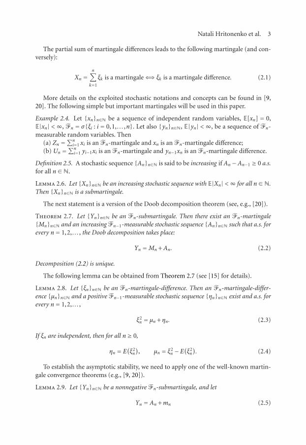
The partial sum of martingale differences leads to the following martingale (and con-versely):
Xn =n∑
k=1
ξk is a martingale⇐⇒ ξk is a martingale difference. (2.1)
More details on the exploited stochastic notations and concepts can be found in [9,20]. The following simple but important martingales will be used in this paper.
Example 2.4. Let {xn}n∈N be a sequence of independent random variables, E[xn] = 0,E|xn| <∞, �n = σ{ξi : i= 0,1, . . . ,n}. Let also {yn}n∈N, E|yn| <∞, be a sequence of �n-measurable random variables. Then
(a) Zn =∑n
i=1 xi is an �n-martingale and xn is an �n-martingale difference;(b) Un =
∑ni=1 yi−1xi is an �n-martingale and yn−1xn is an �n-martingale difference.
Definition 2.5. A stochastic sequence {An}n∈N is said to be increasing if An−An−1 ≥ 0 a.s.for all n∈N.
Lemma 2.6. Let {Xn}n∈N be an increasing stochastic sequence with E|Xn| <∞ for all n∈N.Then {Xn}n∈N is a submartingale.
The next statement is a version of the Doob decomposition theorem (see, e.g., [20]).
Theorem 2.7. Let {Yn}n∈N be an �n-submartingale. Then there exist an �n-martingale{Mn}n∈N and an increasing �n−1-measurable stochastic sequence {An}n∈N such that a.s. forevery n= 1,2, . . . , the Doob decomposition takes place:
Yn =Mn +An. (2.2)
Decomposition (2.2) is unique.
The following lemma can be obtained from Theorem 2.7 (see [15] for details).
Lemma 2.8. Let {ξn}n∈N be an �n-martingale-difference. Then an �n-martingale-differ-ence {μn}n∈N and a positive �n−1-measurable stochastic sequence {ηn}n∈N exist and a.s. forevery n= 1,2, . . . ,
ξ2n = μn +ηn. (2.3)
If ξn are independent, then for all n≥ 0,
ηn = E(ξ2n
), μn = ξ2
n −E(ξ2n
). (2.4)
To establish the asymptotic stability, we need to apply one of the well-known martin-gale convergence theorems (e.g., [9, 20]).
Lemma 2.9. Let {Yn}n∈N be a nonnegative �n-submartingale, and let
Yn =An +mn (2.5)
4 Stability analysis of stochastic Ricker population model
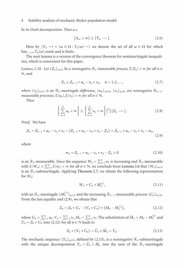
be its Doob decomposition. Then a.s.
{A∞ <∞}⊆ {Yn −→
}. (2.6)
Here by {Yn →} = {ω ∈ Ω : Yn(ω) →} we denote the set of all ω ∈ Ω for whichlimt→+∞Yn(ω) exists and is finite.
The next lemma is a version of the convergence theorem for semimartingale inequali-ties, which is convenient for this paper.
Lemma 2.10. Let {Zn}n∈N be a nonnegative �n-measurable process, E|Zn| <∞ for all n∈N, and
Zn ≤ Zn−1 +un− vn + νn, n= 1,2, . . . , (2.7)
where {νn}n∈N is an �n-martingale difference, {un}n∈N, {vn}n∈N are nonnegative �n−1-measurable processes, E|un|,E|vn| <∞ for all n∈N.
Then{ ∞∑
n=1
un <∞}
⊆{ ∞∑
n=1
vn <∞}⋂{
Zn −→}. (2.8)
Proof. We have
Zn = Zn−1 +un− vn + νn−(Zn−1 +un− vn + νn−Zn
)= Zn−1 +un− vn + νn−wn,(2.9)
where
wn = Zn−1 +un− vn + νn−Zn ≥ 0 (2.10)
is an �n-measurable. Since the sequence Wn =∑n
i=1wi is increasing and �n-measurablewith E|Wn| ≤
∑ni=1E|wi| <∞ for all n∈N, we conclude from Lemma 2.6 that {Wn}n∈N
is an �n-submartingale. Applying Theorem 2.7, we obtain the following representationfor Wn:
Wn = Cn +M(1)n , (2.11)
with an �n-martingale {M(1)n }n∈N and the increasing �n−1-measurable process {Cn}n∈N.
From the last equality and (2.9), we obtain that
Zn = Z0 +Un−(Vn +Cn
)+(Mn−M(1)
n
), (2.12)
where Un =∑n
i=1ui, Vn =∑n
i=1 vi, Mn =∑n
i=1 νi. The substitution of Mn =Mn−M(1)n and
Un = Z0 +Un into (2.12) for all n∈N leads to
Zn +(Vn +Cn
)= Un + Mn = Yn. (2.13)
The stochastic sequence {Yn}n∈N, defined by (2.13), is a nonnegative �n-submartingalewith the unique decomposition Yn = Un + Mn into the sum of the �n-martingale
Natali Hritonenko et al. 5
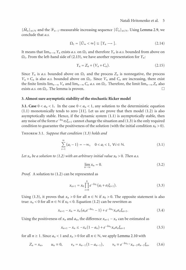
{Mn}n∈N and the �n−1-measurable increasing sequence {Un}n∈N. Using Lemma 2.9, weconclude that a.s.
Ω1 ={U∞ <∞}⊆ {Yn −→
}. (2.14)
It means that limn→∞Yn exists a.s. on Ω1 and therefore Yn is a.s. bounded from above onΩ1. From the left-hand side of (2.13), we have another representation for Yn:
Yn = Zn +(Vn +Cn
). (2.15)
Since Yn is a.s. bounded above on Ω1 and the process Zn is nonnegative, the processVn + Cn is also a.s. bounded above on Ω1. Since Vn and Cn are increasing, there existthe finite limits limn→∞Vn and limn→∞Cn a.s. on Ω1. Therefore, the limit limn→∞Zn alsoexists a.s. on Ω1. The lemma is proven. �
3. Almost sure asymptotic stability of the stochastic Ricker model
3.1. Case 0 < an < 1. In the case 0 < an < 1, any solution to the deterministic equation(1.1) monotonically tends to zero [11]. Let us are prove that then model (1.2) is alsoasymptotically stable. Hence, if the dynamic system (1.1) is asymptotically stable, thenany noise of the form e−bxiσiξi+1 cannot change the situation and (1.3) is the only requiredcondition to guarantee the positiveness of the solution (with the initial condition x0 > 0).
Theorem 3.1. Suppose that condition (1.3) holds and
∞∑
i=1
(ai− 1
)=−∞, 0 < ai < 1, ∀i∈N. (3.1)
Let xn be a solution to (1.2) with an arbitrary initial value x0 > 0. Then a.s.
limn→∞xn = 0. (3.2)
Proof. A solution to (1.2) can be represented as
xn+1 = x0
n∏
i=0
e−bxi(ai + σiξi+1
). (3.3)
Using (1.3), it proves that xn > 0 for all n ∈ N if x0 > 0. The opposite statement is alsotrue: xn < 0 for all n∈N if x0 < 0. Equation (1.2) can be rewritten as
xn+1− xn = xn(ane
−bxn − 1)
+ e−bxnxnσnξn+1. (3.4)
Using the positiveness of xn and an, the difference xn+1− xn can be estimated as
xn+1− xn ≤−xn(1− an
)+ e−bxnxnσnξn+1 (3.5)
for all n≥ 1. Since an < 1 and xn > 0 for all n∈N, we apply Lemma 2.10 with
Zn = xn, un ≡ 0, vn = xn−1(1− an−1
), νn ≡ e−bxn−1xn−1σn−1ξn, (3.6)
6 Stability analysis of stochastic Ricker population model
and obtain that limn→∞ xn a.s. exists and a.s.
∞∑
i=1
xi(1− ai
)<∞. (3.7)
To prove that a.s. limn→∞ xn = 0, we assume the opposite: limn→∞ xn(ω) ≥ c(ω) > 0 forω ∈Ω1, Ω1 ⊂Ω, P{Ω1} > 0. Then, the a.s. finite N =N(ω) exists such that for all n≥N ,and for ω ∈Ω1 we have
∞∑
i=Nxi(ω)
(1− ai
)≥ c(ω)∞∑
i=N
(1− ai
)−→∞ (3.8)
that contradicts our assumption. Hence, the theorem is proven. �
3.2. Case an ≥ 1. In the case an ≥ 1 the zero equilibrium state of the original determin-istic equation is unstable, the population grows and may possess a positive equilibriumstate (e.g., [6, 11]). Let us estimate the lower limit of the solution to the stochastic equa-tion (1.2).
Theorem 3.2. Suppose that condition (1.3) holds, an ≥ 1 for all n > 0, and limn→∞ lnanexists. Let xn be a solution to (1.2) with an arbitrary initial value x0 > 0. Then a.s.
0≤ liminfn→∞ xn ≤ lim
n→∞lnanb
. (3.9)
Proof. Suppose that (3.9) is incorrect, then there exist a set Ω1 ∈Ω and a.s. finite randomvariables δ = δ(ω) > 0 and N =N(ω) such that P(Ω1) > 0 and for n≥N(ω), ω ∈Ω1,
xn(ω)≥ lnanb
+ δ(ω). (3.10)
Then, for any ω ∈Ω1 and n≥N(ω), we have
eb(xn(ω)−δ(ω)) ≥ an, 1− ane−bxn(ω) ≥ 1− e−δ(ω)b = ε(ω) > 0. (3.11)
Since the solution xn to (1.2) is nonnegative, we get
xn(ω)(1− ane
−bxn(ω))≥ 0 (3.12)
for any n≥N(ω) and ω∈Ω1. Let us take
χ(u)=⎧⎨
⎩1, if u > 0,
0, otherwise,(3.13)
and rewrite (3.4) as follows:
xn+1− xn = xn(ane
−bxn − 1)χ[ane
−bxn − 1]
− xn(1− ane
−bxn)χ[1− ane
−bxn]+ e−bxnxnσnξn+1.(3.14)
Natali Hritonenko et al. 7
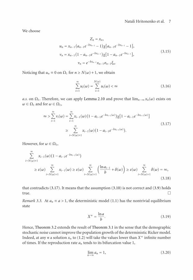
We choose
Zn = xn,
un = xn−1(an−1e
−bxn−1 − 1)χ[an−1e
−bxn−1 − 1],
vn = xn−1(1− an−1e
−bxn−1)χ[1− an−1e
−bxn−1],
νn = e−bxn−1xn−1σn−1ξn.
(3.15)
Noticing that un ≡ 0 on Ω1 for n≥N(ω) + 1, we obtain
∞∑
i=1
ui(ω)=N(ω)∑
i=1
ui(ω) <∞ (3.16)
a.s. on Ω1. Therefore, we can apply Lemma 2.10 and prove that limn→∞ xn(ω) exists onω ∈Ω1 and for ω ∈Ω1,
∞ >∞∑
i=1
vi(ω)=∞∑
i=1
xi−1(ω)(1− ai−1e
−bxi−1(ω))χ[1− ai−1e
−bxi−1(ω)]
≥∞∑
i=N(ω)+1
xi−1(ω)(1− ai−1e
−bxi−1(ω)).
(3.17)
However, for ω ∈Ω1,
∞∑
i=N(ω)+1
xi−1(ω)(1− ai−1e
−bxi−1(ω))
≥ ε(ω)∞∑
i=N(ω)+1
xi−1(ω)≥ ε(ω)∞∑
i=N(ω)+1
(lnai−1
b+ δ(ω)
)≥ ε(ω)
∞∑
i=N(ω)+1
δ(ω)=∞,
(3.18)
that contradicts (3.17). It means that the assumption (3.10) is not correct and (3.9) holdstrue. �
Remark 3.3. At an ≡ a > 1, the deterministic model (1.1) has the nontrivial equilibriumstate
X∗ = lnab
. (3.19)
Hence, Theorem 3.2 extends the result of Theorem 3.1 in the sense that the demographicstochastic noise cannot improve the population growth of the deterministic Ricker model.Indeed, at any n a solution xn to (1.2) will take the values lower than X∗ infinite numberof times. If the reproduction rate an tends to its bifurcation value 1,
limn→∞an = 1, (3.20)
8 Stability analysis of stochastic Ricker population model
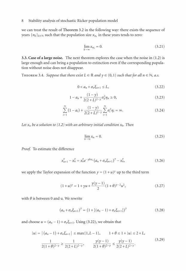
we can treat the result of Theorem 3.2 in the following way: there exists the sequence ofyears {nk}k∈N such that the population size xnk in these years tends to zero:
limk→∞
xnk = 0. (3.21)
3.3. Case of a large noise. The next theorem explores the case when the noise in (1.2) islarge enough and can bring a population to extinction even if the corresponding popula-tion without noise does not disappear.
Theorem 3.4. Suppose that there exist L∈R and γ ∈ (0,1) such that for all n∈N, a.s.
0 < an + σnξn+1 ≤ L, (3.22)
1− an +(1− γ)
2(2 +L)2−γ σ2nηn ≥ 0, (3.23)
∞∑
i=1
(1− ai
)+
(1− γ)2(2 +L)2−γ
∞∑
i=1
σ2i ηi =∞. (3.24)
Let xn be a solution to (1.2) with an arbitrary initial condition x0. Then
limn→∞xn = 0. (3.25)
Proof. To estimate the difference
xγn+1− x
γn = x
γne−γbxn
(an + σnξn+1
)γ − xγn, (3.26)
we apply the Taylor expansion of the function y = (1 +u)γ up to the third term
(1 +u)γ = 1 + γu+γ(γ− 1)
2(1 + θ)γ−2u2, (3.27)
with θ is between 0 and u. We rewrite
(an + σnξn+1
)γ = (1 + [(an− 1) + σnξn+1])γ
(3.28)
and choose u= (an− 1) + σnξn+1. Using (3.22), we obtain that
|u| = ∣∣(an− 1)
+ σnξn+1∣∣≤max{1,L− 1}, 1 + θ ≤ 1 + |u| ≤ 2 +L,
12(1 + θ)2−γ ≥
12(2 +L)2−γ ,
γ(γ− 1)2(1 + θ)2−γ ≤
γ(γ− 1)2(2 +L)2−γ .
(3.29)

Natali Hritonenko et al. 9
Then
xγn+1− x
γn = x
γne−γbxn
(
1 + γ(an− 1
)+
γ(γ− 1)2(2 + θ)2−γ
[(an− 1
)+ σnξn+1
]2)
− xγn
≤ xγne−γbxn
(
1 + γ(an− 1
)+
γ(γ− 1)2(2 +L)2−γ
[(an− 1
)+ σnξn+1
]2)
− xγn
= xγne−γbxn
(
1 + γ(an− 1
)+
γ(γ− 1)2(2 +L)2−γ
[(an− 1
)2+ σ2
nηn+1])
+ μn+1− xγn
≤ xγne−γbxn
(
− γ(1− an
)− γ(1− γ)2(2 +L)2−γ σ
2nηn+1
)
+ xγn(e−γbxn − 1
)+ μn+1
≤−xγneγbxn(
γ(1− an
)+
γ(1− γ)2(2 +L)2−γ σ
2nηn+1
)
+ μn+1,
(3.30)
where
μn+1 = γxγneγbxn
(
σnξn+1 +(γ− 1)
2(2 +L)2−γ[2(an− 1)σnξn+1 + σ2
nμn+1])
. (3.31)
Then, for all n∈N,
xγn+1− x
γn ≤−xγneγbxn
(
γ(1− an
)+
γ(1− γ)2(2 +L)2−γ σ
2nηn+1
)
+ μn+1. (3.32)
Since xn > 0 for all n ∈ N, the first term in the right-hand side of (3.32) is nonpositive.Hence we can apply Lemma 2.10 to inequality (3.32) with
Zn = xγn, un ≡ 0, vn = x
γn−1e
γbxn−1
(
γ(1− an−1
)+
γ(1− γ)2(2 +L)2−γ σ
2n−1ηn
)
,
νn = μn,
(3.33)
and obtain that a.s. limn→∞ xn exists and a.s.
n∑
i=1
xγi e−γbxi
(
1− ai +(1− γ)
2(2 + θ)2−γ σ2i ηi+1
)
<∞. (3.34)
To prove that limn→∞ xn = 0, we assume the opposite: limn→∞ xn(ω) > 0 for ω∈Ω1, Ω1 ⊂Ω, P{Ω1} > 0. Then there exist a.s. finite numbers N = N(ω) > 0 and ζ = ζ(ω) > 0 suchthat for n≥N and ω ∈Ω1,
xn(ω)e−γbxn(ω) ≥ ζ(ω). (3.35)

10 Stability analysis of stochastic Ricker population model
Applying (3.24), we obtain a contradiction to (3.34): on Ω1,
n∑
i=N(ω)
xi(ω)e−γbxi(ω)((
1− ai)
+(1− γ)
2(2 +L)2−γ σ2i ηi+1
)
≥ ζ(ω)n∑
i=N(ω)
((1− ai
)+
(1− γ)2(2 +L)2−γ σ
2i ηi+1
)−→∞, when n−→∞.
(3.36)
It proves the theorem. �
Remark 3.5. If an ≥ 1 and limn→∞ an = 1, then Theorem 3.2 helps to eliminate condition(3.24). Indeed, in this case Theorem 3.2 states that liminfn→∞ xn = 0. From the proof ofTheorem 3.4 it is clear that we need only condition (3.23) for the existence of limn→∞ xn.If it is valid, then limn→∞ xn = 0.
In particular, it means that in the case an ≥ 1, limn→∞ an = 1, the intensity of the noisethat stabilizes (1.2) can be smaller than in the general case. For example, let us choose
an = 1 +1n2
, P{ξn = 1
}= 12
, P{ξn =−1
}= 12
, σn = 8n
, (3.37)
for all n∈N. Then Eξn = 0, Eξ2n = 1, for all n∈N, and
0 < 1 +1n2− 8n≤ an + σnξn ≤ 1 +
1n2
+8n≤ 2 (3.38)
for sufficiently large n. Taking L= 2 and γ = 1/2, we prove that condition (3.23) is valid:
1− an +(1− γ)
2(2 +L)2−γ σ2nηn+1 =− 1
n2+
12243/2
26
n2= 1
n2> 0. (3.39)
However, condition (3.24) is not true.
Remark 3.6. Conditions (3.23), (3.24) hold true, in particular, when the reproductionrates ai are small:
ai ≤ 1, ∀i∈N,∞∑
i=1
(1− ai
)=∞. (3.40)
This case reflects a deteriorating deterministic system and is trivial. Then (3.23) and(3.24) are valid for any noise. It means that Theorem 3.1 is a partial case of Theorem 3.4.
If the sign of ai− 1 is unknown, then the deterministic population with no noise cangrow (in particular, when all an ≥ 1 [11]). Then Theorem 3.4 can provide the restrictionson the reproduction rates ai and the noise intensities σn, ηn when the stochastic popula-tion does not grow but disappears.
One can see that condition (3.23) is valid for some γ ∈ (0,1) if for all n∈N a.s.
an ≤ 1 + kσ2nηn = 1 +Δn, (3.41)
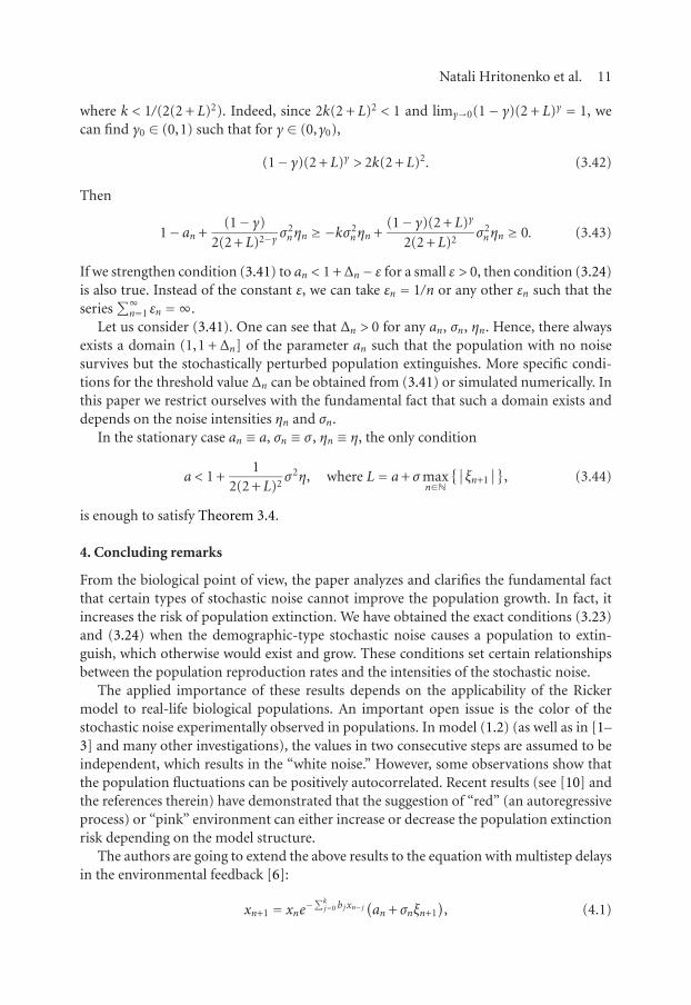
Natali Hritonenko et al. 11
where k < 1/(2(2 + L)2). Indeed, since 2k(2 + L)2 < 1 and limγ→0(1− γ)(2 + L)γ = 1, wecan find γ0 ∈ (0,1) such that for γ ∈ (0,γ0),
(1− γ)(2 +L)γ > 2k(2 +L)2. (3.42)
Then
1− an +(1− γ)
2(2 +L)2−γ σ2nηn ≥−kσ2
nηn +(1− γ)(2 +L)γ
2(2 +L)2σ2nηn ≥ 0. (3.43)
If we strengthen condition (3.41) to an < 1 +Δn− ε for a small ε > 0, then condition (3.24)is also true. Instead of the constant ε, we can take εn = 1/n or any other εn such that theseries
∑∞n=1 εn =∞.
Let us consider (3.41). One can see that Δn > 0 for any an, σn, ηn. Hence, there alwaysexists a domain (1,1 +Δn] of the parameter an such that the population with no noisesurvives but the stochastically perturbed population extinguishes. More specific condi-tions for the threshold value Δn can be obtained from (3.41) or simulated numerically. Inthis paper we restrict ourselves with the fundamental fact that such a domain exists anddepends on the noise intensities ηn and σn.
In the stationary case an ≡ a, σn ≡ σ , ηn ≡ η, the only condition
a < 1 +1
2(2 +L)2σ2η, where L= a+ σmax
n∈N{∣∣ξn+1
∣∣}, (3.44)
is enough to satisfy Theorem 3.4.
4. Concluding remarks
From the biological point of view, the paper analyzes and clarifies the fundamental factthat certain types of stochastic noise cannot improve the population growth. In fact, itincreases the risk of population extinction. We have obtained the exact conditions (3.23)and (3.24) when the demographic-type stochastic noise causes a population to extin-guish, which otherwise would exist and grow. These conditions set certain relationshipsbetween the population reproduction rates and the intensities of the stochastic noise.
The applied importance of these results depends on the applicability of the Rickermodel to real-life biological populations. An important open issue is the color of thestochastic noise experimentally observed in populations. In model (1.2) (as well as in [1–3] and many other investigations), the values in two consecutive steps are assumed to beindependent, which results in the “white noise.” However, some observations show thatthe population fluctuations can be positively autocorrelated. Recent results (see [10] andthe references therein) have demonstrated that the suggestion of “red” (an autoregressiveprocess) or “pink” environment can either increase or decrease the population extinctionrisk depending on the model structure.
The authors are going to extend the above results to the equation with multistep delaysin the environmental feedback [6]:
xn+1 = xne−∑k
j=0 bjxn− j(an + σnξn+1
), (4.1)
12 Stability analysis of stochastic Ricker population model
where k ∈ N is some fixed number, bj ≥ 0 for all i = 0,1, . . . ,k, and ξn+1 are positivelyautocorrelated, and also to the continuous-time case of Ito type integral equations withdistributed delays.
References
[1] H. Fagerholm and G. Hognas, Stability classification of a Ricker model with two random parame-ters, Advances in Applied Probability 34 (2002), no. 1, 112–127.
[2] M. Gyllenberg, G. Hognas, and T. Koski, Null recurrence in a stochastic Ricker model, Analysis,Algebra, and Computers in Mathematical Research (Lulea, 1992) (M. Gyllenberg and L. Persson,eds.), Lecture Notes in Pure and Appl. Math., vol. 156, Marcel Dekker, New York, 1994, pp. 147–164.
[3] , Population models with environmental stochasticity, Journal of Mathematical Biology32 (1994), no. 2, 93–108.
[4] F. C. Hoppensteadt and C. S. Peskin, Mathematics in Medicine and the Life Sciences, Texts inApplied Mathematics, vol. 10, Springer, New York, 1992.
[5] N. Hritonenko and Y. Yatsenko, Mathematical Modeling in Economics, Ecology and the Environ-ment, Kluwer Academic, Dordrecht, 1999.
[6] , Applied Mathematical Modelling of Engineering Problems, Applied Optimization, vol.81, Kluwer Academic, Massachusetts, 2003.
[7] G. Kersting, On recurrence and transience of growth models, Journal of Applied Probability 23(1986), no. 3, 614–625.
[8] V. Kolmanovskii and L. Shaikhet, General method of Lyapunov functionals construction for sta-bility investigation of stochastic difference equations, Dynamical Systems and Applications, WorldSci. Ser. Appl. Anal., vol. 4, World Scientific, New Jersey, 1995, pp. 397–439.
[9] R. Sh. Liptser and A. N. Shiryayev, Theory of Martingales, Mathematics and Its Applications(Soviet Series), vol. 49, Kluwer Academic, Dordrecht, 1989.
[10] J. M. Morales, Viability in a pink environment: why “white noise” models can be dangerous, Ecol-ogy Letters 2 (1999), no. 4, 228–232.
[11] J. D. Murray, Mathematical Biology, Biomathematics, vol. 19, Springer, Berlin, 1989.[12] W. E. Ricker, Stock and recruitment, Journal of Fisheries Research Board of Canada 11 (1954),
559–623.[13] A. Rodkina, On asymptotic behaviour of solutions of stochastic difference equations, Nonlinear
Analysis. Theory, Methods & Applications. Series A: Theory and Methods 47 (2001), no. 7,4719–4730, Proceedings of the Third World Congress of Nonlinear Analysts, Part 7 (Catania,2000).
[14] A. Rodkina and G. Berkolaiko, On asymptotic behavior of solutions to linear discrete stochasticequation, Proceedings of the International Conference “2004-Dynamical Systems and Applica-tions”, Antalya, July 2004, pp. 614–623.
[15] A. Rodkina and X. Mao, On boundedness and stability of solutions of nonlinear difference equationwith nonmartingale type noise, Journal of Difference Equations and Applications 7 (2001), no. 4,529–550.
[16] A. Rodkina, X. Mao, and V. Kolmanovskii, On asymptotic behaviour of solutions of stochasticdifference equations with Volterra type main term, Stochastic Analysis and Applications 18 (2000),no. 5, 837–857.
[17] A. Rodkina and H. Schurz, A theorem on global asymptotic stability of solutions to nonlinear sto-chastic difference equations with Volterra type noises, Stability and Control: Theory and Applica-tions 6 (2004), no. 1, 23–34.
[18] , Global asymptotic stability of solutions of cubic stochastic difference equations, Advancesin Difference Equations 2004 (2004), no. 3, 249–260.

Natali Hritonenko et al. 13
[19] , On global asymptotic stability of solutions of some in-arithmetic-mean-sense monotonestochastic difference equations in R1, International Journal of Numerical Analysis and Modeling2 (2005), no. 3, 355–366.
[20] A. N. Shiryaev, Probability, 2nd ed., Graduate Texts in Mathematics, vol. 95, Springer, New York,1996.
Natali Hritonenko: Department of Mathematics, Prairie View A & M University,P.O. Box 4189, Prairie View, TX 77446, USAE-mail address: [email protected]
Alexandra Rodkina: Department of Mathematics and Computer Science,University of the West Indies, Mona, Kingston 7, JamaicaE-mail address: [email protected]
Yuri Yatsenko: College of Business and Economics, Houston Baptist University,7502 Fondren Road, Houston, TX 77074, USAE-mail address: [email protected]

Submit your manuscripts athttp://www.hindawi.com
Hindawi Publishing Corporationhttp://www.hindawi.com Volume 2014
MathematicsJournal of
Hindawi Publishing Corporationhttp://www.hindawi.com Volume 2014
Mathematical Problems in Engineering
Hindawi Publishing Corporationhttp://www.hindawi.com
Differential EquationsInternational Journal of
Volume 2014
Applied MathematicsJournal of
Hindawi Publishing Corporationhttp://www.hindawi.com Volume 2014
Probability and StatisticsHindawi Publishing Corporationhttp://www.hindawi.com Volume 2014
Journal of
Hindawi Publishing Corporationhttp://www.hindawi.com Volume 2014
Mathematical PhysicsAdvances in
Complex AnalysisJournal of
Hindawi Publishing Corporationhttp://www.hindawi.com Volume 2014
OptimizationJournal of
Hindawi Publishing Corporationhttp://www.hindawi.com Volume 2014
CombinatoricsHindawi Publishing Corporationhttp://www.hindawi.com Volume 2014
International Journal of
Hindawi Publishing Corporationhttp://www.hindawi.com Volume 2014
Operations ResearchAdvances in
Journal of
Hindawi Publishing Corporationhttp://www.hindawi.com Volume 2014
Function Spaces
Abstract and Applied AnalysisHindawi Publishing Corporationhttp://www.hindawi.com Volume 2014
International Journal of Mathematics and Mathematical Sciences
Hindawi Publishing Corporationhttp://www.hindawi.com Volume 2014
The Scientific World JournalHindawi Publishing Corporation http://www.hindawi.com Volume 2014
Hindawi Publishing Corporationhttp://www.hindawi.com Volume 2014
Algebra
Discrete Dynamics in Nature and Society
Hindawi Publishing Corporationhttp://www.hindawi.com Volume 2014
Hindawi Publishing Corporationhttp://www.hindawi.com Volume 2014
Decision SciencesAdvances in
Discrete MathematicsJournal of
Hindawi Publishing Corporationhttp://www.hindawi.com
Volume 2014 Hindawi Publishing Corporationhttp://www.hindawi.com Volume 2014
Stochastic AnalysisInternational Journal of


![Stability and Sensitivity Analysis of Stochastic Programs with … · programming and stochastic programming [14,15,18,19,25{27,30,31]. From practical viewpoint, this kind of stability](https://img.dokumen.tips/doc/110x75/5f41940087b9941f2221071b/stability-and-sensitivity-analysis-of-stochastic-programs-with-programming-and-stochastic.jpg)