STABILITY ANALYSIS OF AN EPIDEMIC MODEL … models, Stability, Treatment, External Source. ـــــــــــــــــــــــــــ ... well as global stability analysis

International Journal of Scientific & Engineering Research, Volume 5, Issue 6, June-2014 767 ISSN 2229-5518

IJSER © 2014 http://www.ijser.org

Stability Analysis of an SSII∗ Epidemic Model with Limited Treatment

Ahmed A. Muhseen

Abstract: There are many factors effect on the spread of infectious disease or control it, some of these factors is (treatment). And there are other factors that help the evolution of infectious diseases, for example (Negligence of the disease or mistake diagnosis of the disease). The main objective of this paper is to study the effect of those factors on the dynamical behavior of a SSII ∗ model. The impact of contact between of population and external sources of disease for example (air and other), on the dynamics of SSII ∗ epidemic model is investigated. The existence, uniqueness and boundedness of the solution of this model are investigated. The local and global dynamical behaviors of the model are studied. Finally, in order to confirm our obtained results and specify the effects of model’s parameters on the dynamical behavior, numerical simulation of the SSII ∗ model is performed.

Keywords: Epidemic models, Stability, Treatment, External Source.

—————————— ——————————

6T1. Introduction The mathematical models have become important tools in analyzing the spread and control of infectious diseases. The development of such models is aimed at both understand observed epidemiological patterns and predicting the consequences of the introduction of public health interventions to control the spread of diseases. Some diseases not confer immunity against the disease but other diseases confer immunity so recovered individuals gain immunity against disease. These types of disease can be modifications by SI and SIS where S susceptible and I infective respectively. Both epidemic models (SI and SIS) are one of the most basic and most important models in describing of many diseases. Therefore, it attached many authors attention and a number of papers have been published. For example Gao and Hethcote [1] considered an SIS model with a standard disease incidence and density-dependent demographics. Li and Ma [2] studied an SIS model with vaccination and temporary immunity. Kermack and Mckendeick [3] proposed a simple SIS model with infective immigrants. In recent years, many papers found treatment function for example, Li et al [4] proposed the SIS model with a limited resource for treatment. Shurowq k. Shafeeq [5] studied the effect of treatment, immigrants and vaccinated on the dynamic of SIS epidemic model. In this paper 6Twe proposed and studied a mathematical model consisting of SSII∗ epidemic model with treatment, in which it is assumed that the disease transmitted by contact as well as external sources in the environment. 6TThe local as well as global stability analysis of this model is investigated.

ــــــــــــــــــــــــــــــــــــــــــــــــــــــــــــــــــــــــــــــــــ• 2TAssistant Lecturer, Ministry of Education, Rusafa\1,

Baghdad-Iraq, Email: [email protected]. 2. The mathematical model Consider a simple epidemiological model in which the total population ( say N(t)) at time t is divided into two sub classes the susceptible individuals S(t) and infected individuals I(t). Such model can be represented as follows:

ISI

dtdI

SSIdtdS

µβ

µβ

−=

−−Λ=

1

1 (1)

Here 0>Λ is the recruitment rate of the population, 0>µ is the natural death rate of the population, 01 >β is

the infected rate (incidence rate) of susceptible individuals due to directed contact with the infected individuals. Now, since there are many infectious disease for example (7TThe flue., 2T7Ttube rculosis2T7T and 2T7Tcholera2T), spread in the environment by different factors including insects, contact or other vectors, therefore, we assumed that the disease in the a above model will transmitted between the population individuals by contact as well as external source of disease in the environment with an external source incidence rate 0≥β . Also it is assumed that the nature recovery rate from infected individuals returns to be susceptible class with a constant rate 0≥α and 0>ψ is the rate of infected individuals from disease I into new disease ∗I . Finally 0,0 2 >> βθ , the disease related death from second disease and the infected rate by contact between the susceptible individuals and infected individuals of second disease respectively. Then if addition above assumption system (1) can be rewritten in the form:

IJSER

http://www.ijser.org/

mailto:[email protected]



( ) ( )

( ) ∗∗∗

∗

+−+=

++−+=

+−++−Λ=

IISIdt

dI

ISIdtdI

ISSIIdtdS

θµψβ

ψµαββ

αµβββ

2

1

21 )(

(2)

Keeping the above in view, in order to study the effect of treatment on the system (2) let T(I) represented the treatment function which given by [4]:

>

≤<=

∗∗

∗∗∗

IIifk

IIifrIIT

0)( (3)

Accordingly, the flow of disease in system (2) along with the above assumptions can be representing in the following block diagram:

Figure (1): Block diagram of system (3). Therefore, system (2) can be modified to:

( ) ( )

( ) )(

)()(

2

1

21

∗∗∗∗

∗∗

−+−+=

++−+=

++−++−Λ=

ITIISIdt

dI

ISIdtdI

ITISSIIdtdS

θµψβ

ψµαββ

αµβββ

(4)

her ∗= rIk this means that the treatment rate is proportional to the number of the infected individuals when the capacity of treatment is not reached, and otherwise takes the maximal capacity. Therefore at any point of time t the total number of population be comes )()()()( tItItStN ∗++= . Obviously, due to the

biological meaning of the variables S(t), I(t) and )(tI∗ , system (4) has the domain

( ) 0,0,0,,, 33 ≥≥≥∈= ∗+

∗+ IISRIISR which is positively in

variant for system (4). Clearly, the interaction functions on the right hand said of system (4) are continuously differentiable. In fact they are Liptschizan function on 3

+R . Therefore, the solution of system (4) exits and unique. Further, all solutions of system (4) with non-negative initial conditions are uniformly bounded as shown in the following theorem. Theorem (1): All the solutions of system (1), which are initiate in 3

+R , are uniformly bounded.

Proof: Let ( ))(),(),( tItItS ∗ be any solution of the system (4)

with non-negative initial conditions ( ))0(),0(),0( ∗IIS .

Since )()()( tItItSN ∗++= , then:

dt

dIdtdI

dtdS

dtdN ∗

++=

This gives

( ) ∗∗ −++−Λ= IIISdtdN θµ

So, Λ≤+ NdtdN µ

Now, by using Gronwall Lemma [6], it obtains that:

tt eNetN µµµ

−− +−Λ

≤ )0()1()(

Therefore, ,)(µΛ

≤tN as ∞→t , hence all the solutions of

system (4) that initiate in 3+R are confined in the reign:

Λ

≤∈= +∗

µυ NRIIS :),,( 3

Which complete the proof. 3. Existence of equilibrium point of system (4) The system (4) has at most three biologically feasible points, namely 2,1,0,),,( == ∗ iIISE iiii . The existence conditions for each of these equilibrium points are discussed in the following:

1) If 0=I and 0=∗I , then the system (4) has an equilibrium point called a disease free equilibrium point and denoted by )0,0,( 00 SE = where:

µΛ

=0S (5)

2) If 0=∗I , then the system (4) has an equilibrium point called a second disease free equilibrium point and denoted by )0,,( 111 ISE = where 11 IandS represented the positive solution of the following set of equations:

( )

( ) ( )

=+−+=+−+−Λ

00

1

1ISI

ISSIµαββ

αµββ

(6)

From equation (1) of above system we get:

µββ

α++

+Λ=

11

11 I

IS

(7a)

Substituting 1S in equation (2) of system (6) we get:

3122

11

21 4

21

2DDD

DDDI −−

−= (7b)

her:

( )Λ=

++−Λ=−=

βµαβµβ

µβ

3

12

11

DDD

Clearly, equation (7b) has a unique positive root by 1I and

then )( 2E exists uniquely in Int. 3+R if and only if 02 >D .

IJSER




3) If 0≠I and 0≠∗I then the system (4) has an equilibrium point called endemic equilibrium point and denoted by ),,( 2222

∗= IISE where 22 , IS and ∗2I

represented the positive solution of the following set of equations in case )0( ∗∗ << II of equation (3) (treatment function):

( ) ( )( ) 0

00)(

2

1

21

=++−+

=++−+=++−++−Λ

∗∗

∗∗

IrISI

ISIrIISSII

θµψβ

ψµαββαµβββ

(8)

Straightforward computation to solve the above system of equations and from equation (2) and (3) of system (8) gives that:

21

22

)(I

ISββψαµ

+++

=

(9a)

))(()(

)(

2122

2122 IrI

IIIββθµψαµβ

ββψ+++−++

+−=∗

(9b)

While, ∗2I positive root if and only if

))(()( 2122 IrI ββθµψαµβ +++<++

Now, substituting 2S and ∗2I in equation (1) of system (8)

we get: 0423

222

321 =+++ AIAIAIA (10)

her:

[ ]])()(

)([)()(

12

2212111

rrrA

++++++++−++++++=

θµαβψαµψβψαµβψβαβθµβψαµβ

[ ]

[ ][])2(

)())(()()()(2

1

12

122112

αββθµβψαµµβψβψαµβθµββαββββψαµψββ

+Λ+++++++++

−++++Λ+++=rrrA

( )[ ])2)((

)()(

12

112

23

αββθµβψβ

µβµββββθµββψαµ

+++−+

++++++Λ++=

rr

rA

0)(24 <++Λ−= rA θµβ

Clearly, equation (10) has a unique positive root by 2I and

then )( 2E exists uniquely in Int. 3+R if and only if 01 >A

then we have the following three cases: Case (1): If the following conditions hold:

>>

00

3

2AA

(11a)

Case (2): If the following conditions hold:

<<

00

3

2AA

(11b)

Case (3): If the following conditions hold:

<>

00

3

2AA

(11c)

4. Local stability analysis of system (4)

In this section, the local stability analysis of the equilibrium points 2,1,0, =iEi of the system (4) studied as shown in the following theorems. Theorem (2): The disease free equilibrium point

)0,0,( 00 SE = of system (4) is locally asymptotically stable provided that: ψαµβα ++<< 01S (12a) rSr ++<< θµβ 02 (12b) ( )[ ] ( )0201001 2 SrSS βψβψαµβαβ −>−+++− (12c) Proof: The Jacobian matrix of system (4) at )( 0E can be written as: ][

330)(×

= ijaEJ

Where:

( )( )rSaaa

aSaaSraSaa

++−====++−==−=−=+−=

θµβψψαµββ

ββαµβ

02333231

23012221

0213011211

;;00;;

;;)(

Then the characteristic equation of )( 0EJ is given by:

0322

13 =Ω+Ω+Ω+ λλλ (13)

her:

[ ]

( ) ( ))()()( 0201

3322111rSS

aaa++−−++−−+=

++−=Ωθµβψαµβµβ

33223311211222112 aaaaaaaa ++−=Ω

[ ]( )( ) ( )[

( )( ) ])()()()(

020201

0201

1332213322113321123

SrrSSrSS

aaaaaaaaa

βψβθµβψαµβµβθµββαβ

−−++−++−++++−−=

−−=Ω

Further:

( ) ( ) ( )( )[ ]133222111221332211

22112333311

2223322

211

321

aaaaaaaaaaaaaaaaaa

+++−+−+−+−=

Ω−ΩΩ=∆

( ) [ ]( ) [ ]( ) [ ]

( )[ ]020101

201

012

2

22

01

2012

()()()()()(()((

)()()(

)()()(

)()(

SrSSrSS

SrS

rSS

rSS

βψψαµβµββαβθµβψαµβµβψαµβµβθµβ

θµβµβψαµβ

θµβψαµβµβ

−+++−++−−×+++−++−++

++−++−++−−

++−++−++−−

++−+++−+−=

Now, according to (Routh-Hurwitz) criterion [7], ( )0E will be locally asymptotically stable provided that 01 >Ω ;

03 >Ω and 0321 >Ω−ΩΩ=∆ .Clearly, 3,1,0 =>Ω ii provided that conditions (12a)-(12b) hold. While,

,0321 >Ω−ΩΩ=∆ Provided that conditions (12)-(a-c) hold. Hence the proof is complete.

IJSER




Theorem (3): The second disease free equilibrium point )0,,( 111 ISE = of system (4) is locally asymptotically stable

if the following sufficient conditions are satisfied: θβψαβµ −−−−> )(2),(2.max 1211 rSS (14) Proof: The Jacobian matrix of system (4) at )( 1E that denoted by )( 1EJ can be written as: [ ]

331)(×

= ijbEJ

Where:

)(;;0

0;)(;;;)(

12332331

2311221121

121311121111

rSbbbbSbIb

SrbSbIb

++−====++−=+=−=−=++−=

θµβψψαµβββ

ββαµββ

Now, according to Gersgorin theorem [8] if the following condition holds:

∑≠=

>3

1ji

iijii bb

Then all eigenvalues of )( 1EJ exists in the region:

<−∈=℘ ∑≠=

∗∗3

1:

jii

ijii bbUCU

Therefore, according to the given condition (14) all the eigenvalues of )( 1EJ exists in the left half plane and hence,

1E is locally asymptotically stable. Theorem(4): The endemic equilibrium point

),,( 2222∗= IISE of system (4) is locally asymptotically

stable if the following sufficient conditions are satisfied: θβψαβµ −−−−> )(2),(2.max 2221 rSS (15) Proof: The Jacobian matrix of system (4) at )( 2E that denoted by )( 2EJ can be written as: [ ]

332)(×

= ijcEJ

Where:

)(;;

0;)(;;;)(

2233232231

2321222121

22132112222111

rSccIc

cScIcSrcScIIc

++−===

=++−=+=−=−=+++−=

∗

∗

θµβψβ

ψαµβββββαµβββ

Now, according to Gersgorin theorem [8] if the following condition holds:

∑≠=

>3

1ji

iijii cc

Then all eigenvalues of )( 2EJ exists in the region:

<−∈= ∑≠=

∗∗3

1:

jii

ijii ccUCUς

Therefore, according to the given condition (15) all the eigenvalues of )( 2EJ exists in the left half plane and hence,

2E is locally asymptotically stable. 5. Globally stability of system (4) In this section, the global dynamics of system (4) is studied with the help of Lyapunov function as shown in the following theorems. Theorem (5): Assume that, the disease free equilibrium point 0E of system (4) is locally asymptotically stable. Then

the basin of attraction of ( )0E , say 30)( +⊂ REB , it is globally

asymptotically stable if satisfy the following condition: )()( 21

∗∗ +<++ rIISII αβββ (16) Proof: Consider the following positive definite function:

∗++

−−= II

SSSSSV0

001 ln

Clearly, RRV →+3

1 : is a continuously differentiable function such that ,0)0,0,( 01 =SV

and )0,0,(),,(,0),,( 01 SIISIISV ≠∀> ∗∗ . Further we have:

dt

dIdtdI

dtdS

SSS

dtdV ∗

++

−= 01

By simplifying this equation we get:

( ) ( )( ) ∗∗

∗∗

−+−

+−+++−−=

III

SS

rIIIISSSdt

dV

θµ

αβββµ021

20

1

Obviously, 01 <dtdV , for every initial points and then 1V is a

Lyapunov function provided that condition (16) hold. Thus 0E is globally asymptotically stable in the interior of

),( 0EB which means that )( 0EB is the basin of attraction and that complete the proof. Theorem (6): Assume that, the second disease free equilibrium point 1E of system (4) is locally asymptotically

stable. Then the basin of attraction of ( )1E , say 31)( +⊂ REB ,

it is globally asymptotically stable if satisfy the following conditions:

++

−++

<

++−

SI

IS

SISISIIS

1

12

1111 )(4)(

βµβ

βψαµββαβ

(17a)

( ) ( ) ∗∗ ++<+ ISrSIIS )(112 θµψβ (17b) Proof: Consider the following positive definite function:

∗+

−−+

−−= I

IIIII

SSSSSV

111

1112 lnln

IJSER




Clearly, RRV →+3

2 : is a continuously differentiable function such that ,0)0,,( 112 =ISV

and )0,,(),,(,0),,( 112 ISIISIISV ≠∀> ∗∗ . Further we have:

dt

dIdtdI

III

dtdS

SSS

dtdV ∗

+

−

+

−

= 112


( ) ( )( ) ( )

( ) ∗∗∗ ++−++−

−−

−−−−−−−=

IrISIISSSr

IIqIISSqSSqdt

dV

θµψββ 212

21221112

2111

2

)(

With:

SISISIISq

ISq

SIq

)(

;)(;

111112

122

111

ββαβ

βψαµβµβ

++−=

−++=

++=

Therefore, according to condition (17a) it is obtaining that:

( ) ( )[ ]( ) ∗

∗

++−+

+−+−−≤

ISrSI

ISIIqSSqdt

dV

)(1

122

1221112

θµψ

β

Obviously, 02 <dtdV for every initial points satisfying

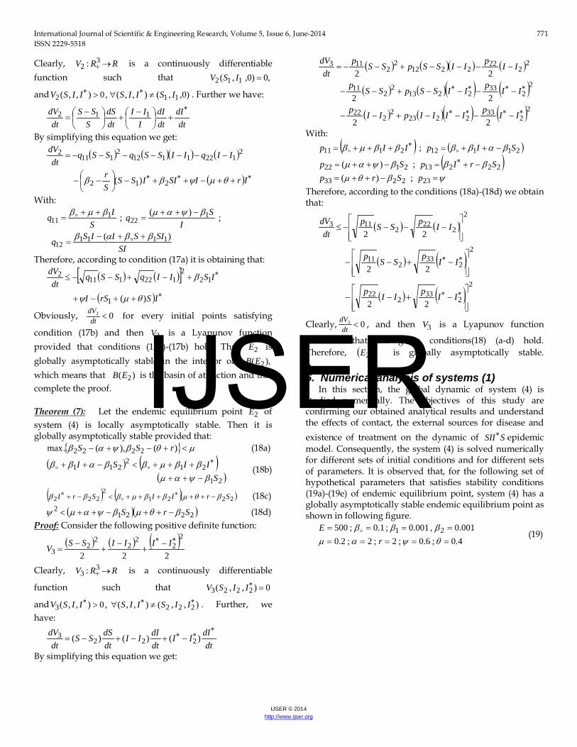
condition (17b) and then 2V is a Lyapunov function provided that conditions (17a)-(17b) hold. Thus 2E is globally asymptotically stable in the interior of ),( 2EB which means that )( 2EB is the basin of attraction and that complete the proof. Theorem (7): Let the endemic equilibrium point 2E of system (4) is locally asymptotically stable. Then it is globally asymptotically stable provided that: µθβψαβ <+−+− )(),(.max 2222 rSS (18a)

( ) ( )( )21

212

211S

IISIβψαµ

ββµββαββ−++

+++<−++ ∗ (18b)

( ) ( )( )22212

222 SrIISrI βθµββµβββ −+++++<−+ ∗∗ (18c)

( )( )22212 SrS βθµβψαµψ −++−++< (18d)

Proof: Consider the following positive definite function:

( ) ( ) ( )222

22

22

22

3∗∗ −

+−

+−

=IIIISSV

Clearly, RRV →+3

3 : is a continuously differentiable

function such that 0),,( 2223 =∗IISV

and ),,(),,(,0),,( 2223∗∗∗ ≠∀> IISIISIISV . Further, we

have:

dt

dIIIdtdIII

dtdSSS

dtdV ∗

∗∗ −+−+−= )()()( 2223


( ) ( )( ) ( )

( ) ( )( ) ( )( ) ( )( ) ( )22

332223

22

22

22

332213

22

11

22

222212

22

113

22

22

22

∗∗∗∗

∗∗∗∗

−−−−+−−

−−−−+−−

−−−−+−−=

IIpIIIIpIIp

IIpIISSpSSp

IIpIISSpSSpdt

dV

With:

( ) ( )( )ψβθµ

βββψαµ

βαββββµβ

=−++=−+=−++=

−++=+++=∗

∗

232233

222132122

211122111

;)(;)(

;

pSrpSrIpSp

SIpIIp

Therefore, according to the conditions (18a)-(18d) we obtain that:

( ) ( )

( ) ( )

( ) ( )2

233

222

2

233

211

2

222

2113

22

22

22

−+−−

−+−−

−−−−≤

∗∗

∗∗

IIpIIp

IIpSSp

IIpSSpdt

dV

Clearly, 03 <dtdV , and then 3V is a Lyapunov function

provided that the given conditions(18) (a-d) hold. Therefore, ( )2E is globally asymptotically stable. 6. Numerical analysis of systems (1) In this section, the global dynamic of system (4) is studied numerically. The objectives of this study are confirming our obtained analytical results and understand the effects of contact, the external sources for disease and existence of treatment on the dynamic of SSII∗ epidemic model. Consequently, the system (4) is solved numerically for different sets of initial conditions and for different sets of parameters. It is observed that, for the following set of hypothetical parameters that satisfies stability conditions (19a)-(19e) of endemic equilibrium point, system (4) has a globally asymptotically stable endemic equilibrium point as shown in following figure.

4.0;6.0;2;2;2.0001.0,001.0;1.0;500 21

=========

θψαµβββ

rE (19)

IJSER




Figure 2- Phase plot and time series of system (4) starting from different initial points. (a) Trajectories of S, started at (3500, 1000, 200) (b) trajectories of I, started at (2000, 4000, 300) (c) trajectories of ∗I started at (1000, 3000, 500). Obviously, Figure (2) shows clearly the convergence of system (4) to the endemic equilibrium point

)154,193,1845(2 =E asymptotically from three different initial points. The effect of increasing the incidence rate of disease resulting from external sources on the dynamics of system (4) is studied by solving the system numerically for the parameters values 4.0,2.0,001.0=β respectively, keeping other parameters fixed as given in equation (19), then the trajectories of system (4) are drawn in Figures (3a)- (3c) respectively and starting at (3500, 2000, 1000).

Figure 3- Time series of the solution of system (4). (a) for 001.0=β , (b) for 2.0=β , (c) for 4.0=β . According to Figure (3), as the incidence rate of disease resulting by external sources increases (through increasing β ), then the trajectory of system (4) approaches asymptotically to the endemic equilibrium point. In fact as β increases it is observed that the number of susceptible

decrease and the number of infected in first disease individuals and infected in second disease individuals increases. Similar results are obtained, as those shown in case of increasing β , in case of increasing the incidence rate of disease resulting by contact between susceptible and infected in first disease, that is means increasing 1β and keeping other parameters fixed as given in (19). The effect of increasing the incidence rate of disease resulting by contact between susceptible and infected in second disease on the dynamics of system (4) is studied by solving the system numerically for the parameters values

006.0,004.0,001.02 =β respectively, keeping other

IJSER




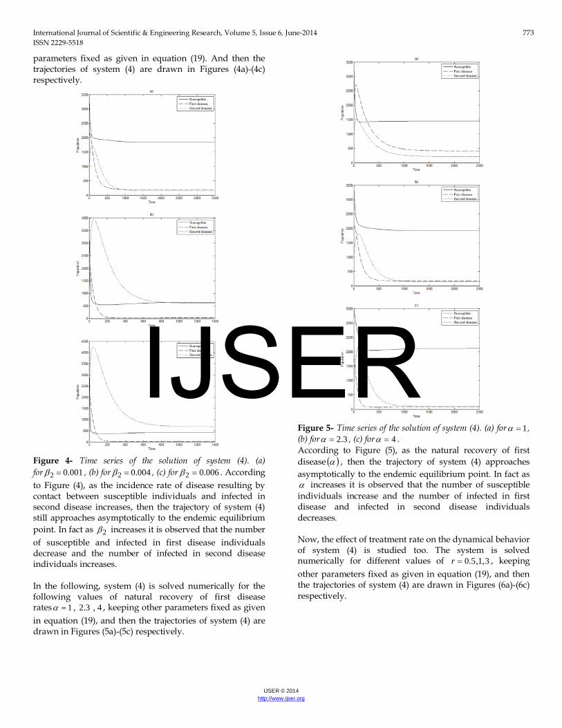
parameters fixed as given in equation (19). And then the trajectories of system (4) are drawn in Figures (4a)-(4c) respectively.

Figure 4- Time series of the solution of system (4). (a) for 001.02 =β , (b) for 004.02 =β , (c) for 006.02 =β . According to Figure (4), as the incidence rate of disease resulting by contact between susceptible individuals and infected in second disease increases, then the trajectory of system (4) still approaches asymptotically to the endemic equilibrium point. In fact as 2β increases it is observed that the number of susceptible and infected in first disease individuals decrease and the number of infected in second disease individuals increases. In the following, system (4) is solved numerically for the following values of natural recovery of first disease rates 4,3.2,1=α , keeping other parameters fixed as given in equation (19), and then the trajectories of system (4) are drawn in Figures (5a)-(5c) respectively.

Figure 5- Time series of the solution of system (4). (a) for 1=α , (b) for 3.2=α , (c) for 4=α . According to Figure (5), as the natural recovery of first disease ( )α , then the trajectory of system (4) approaches asymptotically to the endemic equilibrium point. In fact as α increases it is observed that the number of susceptible individuals increase and the number of infected in first disease and infected in second disease individuals decreases. Now, the effect of treatment rate on the dynamical behavior of system (4) is studied too. The system is solved numerically for different values of 3,1,5.0=r , keeping other parameters fixed as given in equation (19), and then the trajectories of system (4) are drawn in Figures (6a)-(6c) respectively.

IJSER




Figure 6- Time series of the solution of system (4). (a) for 5.0=r , (b) for 1=r , (c) for 3=r . According to Figure (6), as the treatment ( )r , then the trajectory of system (4) approaches asymptotically to the endemic equilibrium point. In fact as r increases it is observed that the number of susceptible and infected in first disease individuals increase and the number of infected in second disease individuals decrease. Similar results are obtained, as those shown in case of increasing r , in case of increasing the disease related death of second disease, that is means increasing θ and keeping other parameters fixed as given in (19). As shown in the following figures (7a)-(7c).

Figure 7- Time series of the solution of system (4). (a) for 2.0=θ , (b) for 5.0=θ , (c) for 8.0=θ . According to Figure (7), the disease related of second disease ( )θ , and then the trajectory of system (4) approaches asymptotically to the endemic equilibrium point. In fact as θ increases it is observed that the number of susceptible and infected in first disease individuals increase and the number of infected in second disease individuals decrease. The effect of the natural death rate on the dynamics of system (4) is investigated numerically. It is observed that, increases the parameter µ and keeping other parameters fixed as in (19) then the trajectory of system (4) approaches asymptotically to the endemic equilibrium point as shown in Figures (8a)-(8b).

IJSER




Figure 8- Time series of the solution of system (4). (a) for 1.0=µ , (b) for 2.0=µ , (c) for 3.0=µ . According to Figure (8), the natural death ( )µ , and then the trajectory of system (4) approach asymptotically to the endemic equilibrium point. In fact as µ increases it is observed that the number of susceptible individuals with the number of infected in first disease and second disease individuals decrease. Finally, the effect of evolution rate of first disease and becomes to second disease that means increasingψ , on the dynamical behavior of system (4) is studied. The system is solved numerically for different values of 9.0,7.0,5.0=ψ , keeping other parameters fixed as given in equation (20) and then the trajectory of system (4) as shown in Figures (9a)-(9c).

Figure 9- Time series of the solution of system (4). (a) for 5.0=ψ , (b) for 7.0=ψ , (c) for 9.0=ψ . According to Figure (9), the evolution rate ( )ψ , and then the trajectory of system (4) approach asymptotically to the endemic equilibrium point. In fact as ψ increases it is observed that the numbers of susceptible individuals and second disease individuals increase with the number of infected in first disease individuals decrease. 7. Conclusion and discussion In this paper, we proposed and analyzed an epidemiological model that described the dynamical behavior of an epidemic model, where the infectious disease transmitted directly from external sources as well as through contact between them. The model included fore non-linear autonomous differential equations that describe the dynamics of three different populations namely susceptible individuals ),(S infected individuals for first disease )(I and infected individuals for second disease

(evolution of first disease) )( ∗I . The boundedness of system (4) has been discussed. The conditions for existence,

IJSER




stability for each equilibrium points are obtained. Further, it is observed that the disease free equilibrium point ( )0E exists when 0=I and locally stable if the conditions are hold (12) and it is globally stable if and only if the condition (16) holds. The second disease free equilibrium point ( )1E exists if ( 02 >D ) holds and locally stable if the conditions (14) are hold while it is globally stable if and only if the conditions (17a)-(17b) hold. The endemic equilibrium point ( )2E exists if 01 >A and one of three conditions is hold (11a or 11b or 11c) and locally stable if the conditions (15) hold more than it is globally stable if and only if the conditions (18a)-(18d) hold. Finally, to understand the effect of varying each parameter on the global system (4) and confirm our above analytical results, the system (4) has been solved numerically for different sets of initial points and different sets of parameters given by equation (19), and the following observations are made:

1. The system (4) do not has periodic dynamic, instead it they approach either to the all equilibrium point.

2. As the incidence rate of disease (external incidence rate ( )β or contact incidence rate ( )1β ) increase, the asymptotic behavior of the systems (4) approaching to endemic equilibrium point. In fact are ( )1,, =iiβ increase it are observed that the number of ( )S

decrease and the number of ( )∗IandI increase.

3. As the incidence rate of disease (contact incidence rate ( )2β ) increase, the asymptotic behavior of the systems (4) approaching to endemic equilibrium point. In fact as ( )2β increase it is observed that the number of ( )IandS decrease and the number of ( )∗I increase.

4. As the natural recovery rate of first disease ( )α the asymptotic behavior of the systems (4) approaching to endemic equilibrium point with increase it is observed that the number of ( )S

increase and the number of ( )∗IandI decrease.

5. As the treatment rate ( )r and the disease related death of second disease ( )θ increase, the asymptotic behavior of the systems (4) approaching to endemic equilibrium point with increase it is observed that the number of ( )IandS increase and the number of ( )∗I decrease.

6. The increase in the natural death rate ( )µ , the asymptotic behavior of the systems (4) approaching to endemic equilibrium point with increase it is observed that the number of each the population ( )∗IandIS , decrease.

7. As the evolution rate )(ψ increase, the asymptotic behavior of the systems (4) approaching to endemic equilibrium point with increase it is observed that the number of

( )∗IandS increase and the number of ( )I decrease.

References:

[1] Gao L.Q., and Hethcote H.W., Disease models of with density-dependent demographics, J. Math. Biol., 50, 17-31, 1995.

[2] Li J., and Ma Z., Qualitative analysis of SIS

epidemic model with vaccination and varying total population size, Math. Comput. Model, 20, 43-1235, 2002.

[3] Kermack W.O., Mckendrick A.G., Contributions to

mathematical theoryof epidemics, Proc. R. Soc. Lond. A., 115, 700-721, 1927.

[4] Li. X.Z. et. al., Stability and bifurcation of an SIS

epidemic model with treatment, J. Chaos, Solution and Fractals, 42, 2822-2832, 2009.

[5] Shurowq k. Shafeeq, (2011). The effect of treatment,

immigrants and vaccinated on the dynamic of SIS epidemic model. M.Sc. thesis. Department of Mathematics, College of Science, University of Baghdad. Baghdad, Iraq.

[6] Hirsch, M. W. and Smale, S. (1974). Differential Equation, Dynamical System, and Linear Algebra. Academic Press, Inc., New York. p 169-170.

[7] May R. M., Stability and Complexity in model

ecosystem, Princeton, New Jersey: Princeton University press, 1973.

[8] Horn R. A., Johanson C. R., matrix analysis,

Cambridge University press, 1985.

IJSER




IJSER


Documents

STABILITY ANALYSIS OF AN EPIDEMIC MODEL … models, Stability, Treatment, External Source. ـــــــــــــــــــــــــــ ... well as global stability analysis