Embed Size (px)
DESCRIPTION
EE457 Lecture Notes
Citation preview

1
Stability 2
1.0 Introduction
We ended our last set of notes, concluding that
the following equation characterizes the electromechanical dynamics of a synchronous
machine.
sin)( 0
d
a
MX
VEPtM
(1)
Now I want to do an example of the most simple power system that we can consider – the so-
called one-machine against an infinite bus.
2.0 Example
Consider the power system in Fig. 1. It is referred to as a one-machine against an infinite
bus. There are no modern day power systems like this, although there are portions of actual
systems which behave in a similar way, and this system serves well to illustrate these basic kinds
of behavior.

2
So many engineers use it to provide conceptual basis for understanding fundamental machine
behavior. It would not be used, however, to provide precise machine response as the
computer serves well for this purpose.
Bus 1 Bus 2 Bus 3
j0.4
j0.4
j0.1 X’d=j0.2
|Vt|= |V1|=1.0
V= 1.0<0°
Fig. 1
Bus 2, the infinite bus, is so-called because it has a voltage and angle that is constant under all
conditions, and it can absorb infinite power. Although there is no real infinite bus in power
systems, a single small machine connected to a very large power system behaves as if it is
connected to an infinite bus.

3
Given that the machine is delivering 1.0 per unit power under steady-state conditions, we have
the following objectives in this problem. 1. Determine the voltage phasor Ea.
2. Draw the power-angle (P-δ) curve.
3. Determine the steady-state operating point
corresponding to the 1.0 pu power
condition on the pre-fault power angle
curve.
4. For a three-phase fault in the middle of one
of the lines between buses 3 and 2,
determine the fault-on power angle curve.
5. Determine the post-fault power-angle curve
after protection has operated to clear the
fault.
6. Determine the steady-state operating point
corresponding to the 1.0 pu power
condition on the post-fault power angle
curve.
7. Use the three curves to describe what
happens to the angle δ during the three
periods: pre-fault, fault-on, and post-fault.
4
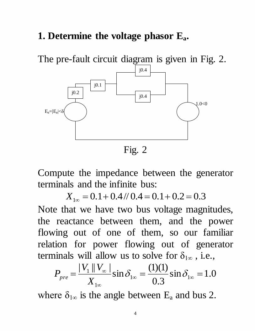
1. Determine the voltage phasor Ea.
The pre-fault circuit diagram is given in Fig. 2.
j0.2
j0.1
j0.4
j0.4
Ea=|Ea|<δ
1.0<0
Fig. 2
Compute the impedance between the generator terminals and the infinite bus:
3.02.01.04.0//4.01.01 X Note that we have two bus voltage magnitudes,
the reactance between them, and the power flowing out of one of them, so our familiar
relation for power flowing out of generator terminals will allow us to solve for δ1∞ , i.e.,
0.1sin3.0
)1)(1(sin
||||11
1
1
X
VVPpre
where δ1∞ is the angle between Ea and bus 2.

5
458.171
458.1711V From this we can compute the current flowing from the machine terminals (bus 1) to the
infinite bus, according to
729.8012.13.0
00.1458.170.1
jI
And from this, we may compute the internal voltage phasor Ea, according to
44.2805.1
)2.0(729.8012.1458.170.1
)2.0(1
j
jIVEa
The above procedure is typical of what is done in full-scale commercial power flow programs
where the program will begin from a power flow solution, from which it computes the
current flow from every gen bus, and then it computes each generator’s internal voltage as
we have done in the above.

6
2. Draw the power-angle (P-δ) curve.
We can draw the power angle curve for different
angles. Some of the choices are given below:
1
1
1 sin||||
X
VVPpre (2)
a
a
apre
X
VEP sin
||||
(3)
2
2
2 sin||||
X
VVPpre (4)
Note that the electrical power (left-hand-side) is
the same in all three cases since there is no resistance in this circuit. We should choose the
most restrictive power angle curve, i.e., the one that gives the largest angle for the same power.
Since the voltages are all reasonably close, the most restrictive curve is determined by the one
with the largest reactance – this would be eq (3).
Using the numerical data for eq. (3), we have:
aaa
a
apre
X
VEP sin1.2sin
5.0
)1)(05.1(sin
||||
(5)
Fig. 3 illustrates this curve.

7
2.2 2.0
1.8 1.6
1.4
1.2 1.0
0.8 0.6
0.4 0.2
0
0 10 20 30 40 50 60 70 80 90 100 110 120 130 140 150 160 170 180 δa
Pe Power
Fig. 3
3. Determine the steady-state operating point
corresponding to the 1.0 pu power
condition on the pre-fault power angle
curve.
This is where Pe=1.0, i.e., 0.1sin1.2 apreP (6)
Solving for δa, we get δa=28.44°. We can
show this point on the pre-fault power-angle curve, using dots as in Fig. 4.

8
2.2 2.0
1.8 1.6
1.4
1.2 1.0
0.8 0.6
0.4 0.2
0
0 10 20 30 40 50 60 70 80 90 100 110 120 130 140 150 160 170 180 δa
●
●
Pe Power
Fig. 4
Figure 4 shows, however, that there are really
two solutions, one at 28.44° and the other at 180-28.44=151.56°. Both of these points
constitute equilibria, i.e., a location in terms of the problem variables where all equations are
satisfied, and, if unperturbed, the system would be able to lie in rest. We shall show later,
however, that the point at 28.44° is a stable equilibrium, and the point at 151.56° is an
unstable equilibrium.

9
4. For a three-phase fault in the middle of one
of the lines between buses 3 and 2,
determine the fault-on power angle curve.
The faulted system is shown in Fig. 5.
Bus 1 Bus 2 Bus 3
j0.4
j0.2
j0.1 X’d=j0.2
|Vt|= |V1|=1.0
V= 1.0<0°
j0.2
Fig. 5 The circuit diagram corresponding to the faulted
system is shown in Fig. 6.
j0.2
j0.1 j0.4
j0.2 Ea=|Ea|<δ
1.0<0
j0.2
Fig. 6

10
So we want to be able to write another equation like eq. (5), except this time, the electrical
power out will not be Ppre but rather Pfault.
To write such an equation, however, we will need the series reactance between the two
voltage sources. This series reactance is not obvious from the circuit diagram of Fig. 6. We
can get it, however, if we replace the circuit to the right of the two marked nodes in Fig. 6 with
its Thevenin equivalent. The relevant part of the circuit is shown in Fig. 7.
j0.4
j0.2
1.0<0
j0.2
Fig. 7
We obtain the Thevenin voltage from the circuit of Fig. 7 as the voltage seen at the left-hand
terminals. We can use voltage division to get it.

11
03333.04.02.0
2.000.1thevV (7)
We get the Thevenin impedance by idling the
source and computing the composite impedance, as shown in Fig. 8.
j0.4
j0.2 j0.2
Fig. 8
In Fig. 8, we recognize that the j0.2 impedance on the right is shorted, therefore the impedance
seen looking in from the terminals on the left is just the parallel combination of the j0.2
impedance on the left and the j0.4 impedance at the top. This is j(0.2)(0.4)/0.6=j0.1333. The
faulted circuit with the Thevenin equivalent is given in Fig. 9.

12
j0.2
j0.1 j0.1333
Ea=|Ea|<δ
0.333<0
Fig. 9
From Fig. 9, we can immediately see that the
impedance between the sources is
4333.01333.01.02.0 aThevX
write down the power-angle equation as:
aThev
aThevaThev
aThev
Thevafault
X
VEP
sin8077.0
sin4333.0
)333.0)(05.1(sin
||||
(8)
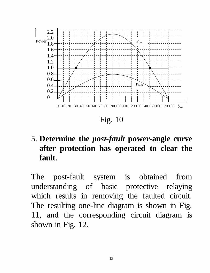
This curve is plotted in Fig. 10.
13
2.2 2.0
1.8 1.6
1.4
1.2 1.0
0.8 0.6
0.4 0.2
0
0 10 20 30 40 50 60 70 80 90 100 110 120 130 140 150 160 170 180 δa
●
●
Ppre
Pfault
Power
Fig. 10
5. Determine the post-fault power-angle curve
after protection has operated to clear the
fault.
The post-fault system is obtained from
understanding of basic protective relaying which results in removing the faulted circuit.
The resulting one-line diagram is shown in Fig. 11, and the corresponding circuit diagram is
shown in Fig. 12.

14
Bus 1 Bus 2 Bus 3
j0.4 j0.1 X’d=j0.2
|Vt|= |V1|=1.0
V= 1.0<0°
Fig. 11
j0.2
j0.1 j0.4
Ea=|Ea|<δ
1.0<0
Fig. 12
Again, we need the series reactance between the
two voltage sources, but this time, it is very easy to see that this series reactance is
7.04.01.02.0 aX
Therefore, the post-fault power-angle curve is given by

15
a
aa
a
apost
X
VEP
sin5.1
sin7.0
)0.1)(05.1(sin
||||
(9)
This curve is plotted in Fig. 13.
2.2 2.0
1.8 1.6
1.4
1.2 1.0
0.8 0.6
0.4 0.2
0
0 10 20 30 40 50 60 70 80 90 100 110 120 130 140 150 160 170 180 δa
●
●
Ppre
Pfault
Ppost
Power
Fig. 13
Note from Fig. 13 that the pre-fault curve is
highest, the fault-on curve is lowest, the post-fault
curve is in between. This reflects the relative
“strength” of the systems to transfer power from
source to the infinite bus, where “strength” is
determined by the impedance magnitude between
source and infinite bus and voltage magnitudes at
these two buses. More transmission makes
systems stronger.

16
6. Determine the steady-state operating point
corresponding to the 1.0 pu power
condition on the post-fault power angle
curve.
This is where Pe=1.0, i.e.,
0.1sin5.1 apostP (6)
Solving for δa, we get δa=41.81°. We can show this point on the pre-fault power-angle
curve using triangles, as in Fig. 14.
2.2 2.0
1.8 1.6
1.4
1.2 1.0
0.8 0.6
0.4 0.2
0
0 10 20 30 40 50 60 70 80 90 100 110 120 130 140 150 160 170 180 δa
●
●
Ppre
Pfault
Ppost
▲
▲
Power
Fig. 14
Again, we see that there are two equlibria.

17
7. Use the three curves to describe what
happens to the angle δ during the three
periods: pre-fault, fault-on, and post-fault.
We have the pre-fault equilibrium (at 28.44°) identifying where this systems “starts” (just
before and just after being faulted) and the post-fault equilibrium (at 41.81°) identifying where
this system “ends” (after fault is cleared and after all transients die out).
Question is: What happens in between these two
points in time?
Let’s review the sequence, to be clear. a. Prefault condition.
b. t=0: fault occurs c. t=4 cycles (typical clearing): fault is cleared
d. t=many seconds: transients die out and system returns to rest.
So we want to know what happens between
steps b and d. Figure 15 tells this story.

18
2.2 2.0
1.8 1.6
1.4
1.2 1.0
0.8 0.6
0.4 0.2
0
0 10 20 30 40 50 60 70 80 90 100 110 120 130 140 150 160 170 180 δa
●
●
Ppre
Pfault
Ppost
▲
▲
(a)
(b)
(d)
(e)
(c)
(f) (g)
Power
Fig. 15
Each stage of Fig. 15 (a, b, c, d, e, f, g) is described in what follows:
(a) On occurrence of the fault, the electrical power out of the machine immediately drops
due to the change in power-angle curves caused by the change in the network (from pre-fault
network, Fig. 2, to the fault-on network, Fig. 9). However, because the power angle δ,
characterizes the mechanical angle of the rotor, it cannot change instantaneously, and therefore
it remains at 28.44° during this transition.

19
(b) Although the electrical power out of the machine has decreased from 1.0 to about 0.4 pu,
the mechanical power into the machine is still 1.0 pu. Therefore the accelerating power
Pa=PM-Pe is no longer zero, rather it is positive (about 0.6), and so the machine begins to
accelerate. This means that its rotational velocity begins to change. Whereas before the
fault, it had a velocity equal to that of the synchronously rotating reference frame (and so
a relative velocity of 0), after the fault, due to acceleration, that velocity begins to increase
(relative velocity increases from 0).
(c) Because the relative velocity is positive,
the angle , which is relative to the reference
angle (the infinite bus angle), increases. (d) At some point in time, let’s say 4 cycles
after the fault, the protective system causes the breakers at both ends of the faulted circuit to
operate and clear the fault. This results in a new network (post-fault, Fig. 12), and
correspondingly a new power-angle curve. But

20
because the angle cannot change instantaneously, it remains at the angle it was at
the moment just before the fault was cleared. Figure 15 indicates this angle is about 60°.
(e) Now the electrical power out of the machine has increased to about 1.3 pu. But the
mechanical power into the machine is still 1.0 pu. Therefore Pa=PM-Pe is negative (about -0.3),
and so the machine begins to decelerate. (f) Because of the acceleration associated with
stage (c), the velocity is still positive and therefore the angle is increasing. But because of
deceleration, the velocity is decreasing. (g) At some point (assuming the behavior is
stable), the velocity becomes zero, and because Pa=PM-Pe is still negative (so machine is still
decelerating), the velocity will go negative. When the velocity goes negative, the angle δ
begins to decrease.
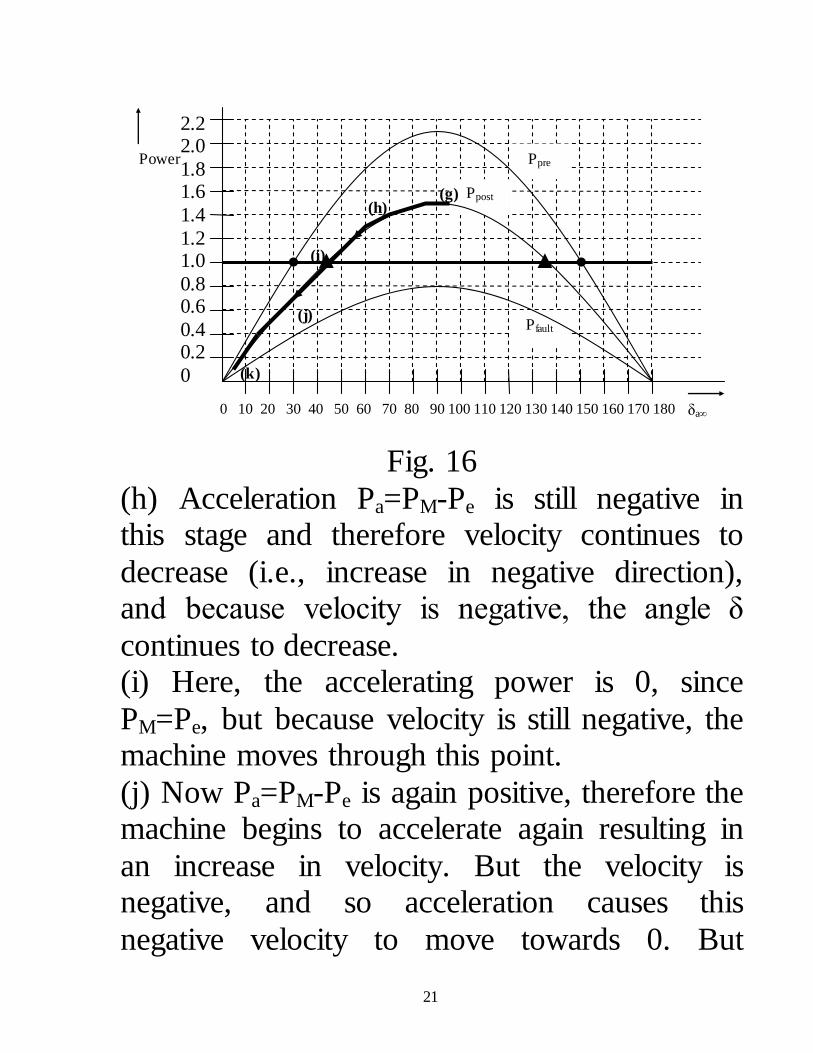
The next stages (h, i, j, k) are shown in Fig. 16.
21
2.2 2.0
1.8 1.6
1.4
1.2 1.0
0.8 0.6
0.4 0.2
0
0 10 20 30 40 50 60 70 80 90 100 110 120 130 140 150 160 170 180 δa
●
●
Ppre
Pfault
Ppost
▲
▲
(g) (h)
(j)
(k)
(i)
Power
Fig. 16
(h) Acceleration Pa=PM-Pe is still negative in this stage and therefore velocity continues to
decrease (i.e., increase in negative direction), and because velocity is negative, the angle δ
continues to decrease. (i) Here, the accelerating power is 0, since
PM=Pe, but because velocity is still negative, the machine moves through this point.
(j) Now Pa=PM-Pe is again positive, therefore the machine begins to accelerate again resulting in
an increase in velocity. But the velocity is negative, and so acceleration causes this
negative velocity to move towards 0. But

22
because the velocity is negative during this stage, the angle δ continues to decrease.
(k) The velocity has reached 0 again, and because Pa=PM-Pe is still positive, the machine
continues to accelerate, and so the velocity becomes positive. As the velocity becomes
positive, the angle begins to increase again.
The next stages, represented by (l, m, n), are shown in Fig. 17.
2.2 2.0
1.8 1.6
1.4
1.2 1.0
0.8 0.6
0.4 0.2
0
0 10 20 30 40 50 60 70 80 90 100 110 120 130 140 150 160 170 180 δa
●
●
Ppre
Pfault
Ppost
▲
▲
(p) (n)
(l)
(k)
(m)
(o)
Power
Fig. 17
(l) Pa=PM-Pe is positive and so the machine continues to accelerate. Velocity is positive, and
so angle increases.

23
(m) Here, Pa=PM-Pe is zero (PM=Pe) but because velocity is positive, machine moves through this
point. (n) Pa=PM-Pe is negative, so machine
decelerates. But velocity is positive, so angle continues to increase. At some point, velocity
reaches 0, and angle begins to decrease. (o) If damping is present, the point at which the
angle begins to decrease (the “turn-around” point) will occur “before” the turn-around point
seen in the previous oscillation. (p) If damping is not present, the “turn around
point” will be the same as the one in the last oscillation (labeled point (p) here but previously
labeled (g)).
One last thing with respect to this example. We have plotted power vs. angle, but you should be
aware that the angle is actually a function of time. This relationship is conveniently
illustrated in Fig. 18, where we also indicate a few stages previously discussed (b, g, i, k).

24
2.2
2.0 1.8
1.6
1.4 1.2
1.0 0.8
0.6 0.4
0.2
0
0 10 20 30 40 50 60 70 80 90 100 110 120 130 140 150 160 170 180 δa
●
●
Ppre
Pfault
Ppost
▲
▲
(b)
(g)
(i)
(k)
Tim
e (
sec)
(b) (g)
(k)
(p)
(o)
(o)
Power
Fig. 18

25
In Fig. 18, the curves extending downwards are using the horizontal axis of the power-angle
curve (the δ-axis) as the vertical axis of the angle-time curve. There are two angle-time
curves shown, and both are associated with stable system behavior. The thin-lined curve
shows the angular oscillation following the disturbance if the system has no damping. Such
a system oscillates forever. The solid-lined curve shows the angular oscillation following
the disturbance if the system has damping. One observes that the amplitude of the oscillations of
this curve diminish with time (this is the realistic case).
3.0 Equilibria
We mentioned on page 8 of these notes that there are two equilibria for our pre-fault system,
as shown in Fig. 4, which is repeated in Fig. 19, except we have designated the two points x and
y. We also indicated that the one at 28.44° (x) is a stable equilibrium, and the one at 180-
28.44=151.56° (y) is an unstable equilibrium.

26
2.2 2.0
1.8 1.6
1.4
1.2 1.0
0.8 0.6
0.4 0.2
0
0 10 20 30 40 50 60 70 80 90 100 110 120 130 140 150 160 170 180 δa
●
● x y
Pe Power
Fig. 19
We can give an analogy here to a ball in a bowl. The stable equilibrium corresponds to when the
ball is resting at the bottom of the bowl. The unstable equilibrium corresponds to when the
ball is resting on the edge of the ball. This is illustrated in Fig. 20a.
Stable equilibrium Unstable equilibrium
Fig. 20a

27
It is possible for the ball to be at rest (in equilibrium) in both positions. However, the
stable equilibrium is resilient to disturbances. If you shake the table, or if you give the ball a
push, the ball in the stable equilibrium will move but then return to the stable equilibrium.
On the other hand, the unstable equilibrium is
not resilient to disturbances. If you shake the table, or if you give the ball a push, the ball in
the unstable equilibrium will move down the bowl and come to rest at the stable equilibrium,
or it will move out of the bowl altogether. If we consider the ball-bowl as a system, the latter
movement is analogous to instability. A metal rod pendulum provides a similar
analogy, shown in Fig. 20b [1].
Fig. 20b

28
We are now in a position to understand why one
is a stable equilibrium and one is an unstable equilibrium. Consider perturbing the machine at
the stable equilibrium, point x. The perturbation could be a fault, but let’s maintain simplicity as
much as possible and assume the perturbation is just a small increase in mechanical power PM.
The key point is that the moment just after the perturbation, the mechanical power is greater
than 1, say 1.1, whereas the electrical power is still 1, and the machine begins to accelerate. The
situation is illustrated in Fig. 21.
2.2
2.0 1.8
1.6 1.4
1.2 1.0
0.8
0.6 0.4
0.2 0
0 10 20 30 40 50 60 70 80 90 100 110 120 130 140 150 160 170 180 δa
●
● x y PM=1.1
Pe Power
PM=1.0
Fig. 21

29
This means the velocity becomes positive and the angle begins to increase.
Question: As the angle increases (the point
begins to move up and to the right, as shown), what happens to the accelerating power?
Answer: Pa=PM-Pe decreases. This means that the rate of change in velocity is decreasing.
Once the point moves above the solid line corresponding to PM=1.1, the machine will
begin to decelerate, i.e., rate of change in velocity will go negative and the velocity will
begin to decrease.
The fact that the perturbation causes acceleration resulting in motion that inherently
decreases that acceleration is the reason this is a stable equilibrium.
One can go through similar logic in relation to
the situation when mechanical power is

30
decreased to, say, 0.9. Then the machine decelerates, the angle decreases, and as angle
decreases, the decelerating power decreases.
Now let’s consider the unstable equilibrium, point y, and let’s again assume a small increase
in mechanical power PM to, say, 1.1 pu. Does the angle increase or decrease?
Because Pa=PM-Pe is positive, the velocity goes positive, resulting in an increase in angle.
Question: As the angle increases (the point
begins to move down and to the right, as shown), what happens to the accelerating
power?
Answer: Pa=PM-Pe increases! This means that the rate of change in velocity is increasing. The
point does not move above the solid line corresponding to PM=1.1, and so the machine
never decelerates. In fact, the accelerating power just continues to increase, equivalent to
the ball falling of the edge.

31
The fact that the perturbation causes
acceleration resulting in motion that inherently increases that acceleration is the reason this is
an unstable equilibrium.
One can go through similar logic in relation to the situation when mechanical power is
decreased to, say, 0.9. Then the machine decelerates, the angle decreases, and as angle
decreases, the decelerating power increases. This will continue until point y moves all the
way back to point x, the stable equilibrium. This is equivalent to the ball rolling down into the
bowl. [1] http://galileospendulum.org/2011/05/31/physics-quanta-pendulums-revisited