STA  4273H:    Sta-s-cal  Machine  Learning    

Russ  Salakhutdinov  Department of Computer Science!Department of Statistical Sciences!

rsalakhu@cs.toronto.edu!h0p://www.cs.utoronto.ca/~rsalakhu/  

Lecture 2  

Last Class •  In our last class, we looked at:

-  Statistical Decision Theory -  Linear Regression Models -  Linear Basis Function Models -  Regularized Linear Regression Models -  Bias-Variance Decomposition

•  We will now look at the Bayesian framework and Bayesian Linear Regression Models.

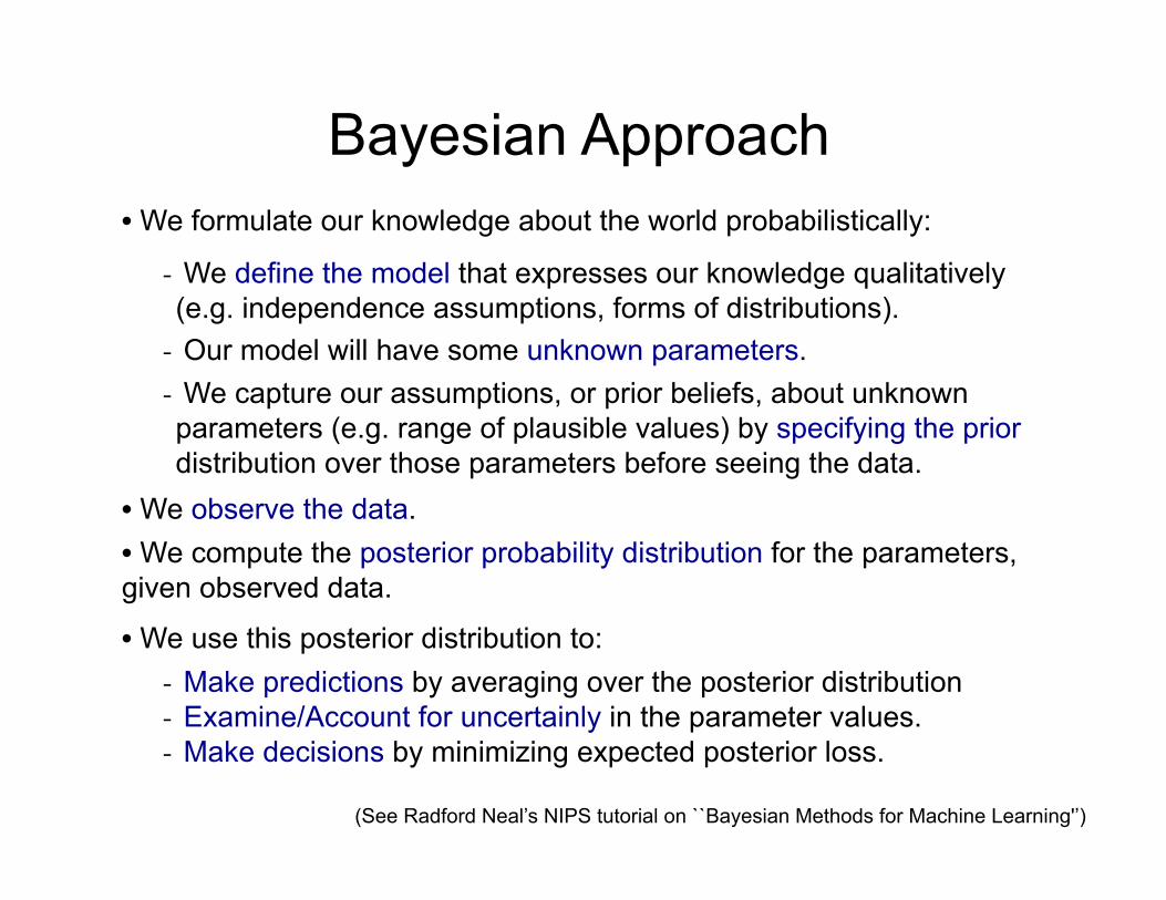
Bayesian Approach •  We formulate our knowledge about the world probabilistically:

-  We define the model that expresses our knowledge qualitatively (e.g. independence assumptions, forms of distributions).

•  We observe the data. •  We compute the posterior probability distribution for the parameters, given observed data.

•  We use this posterior distribution to: -  Make predictions by averaging over the posterior distribution -  Examine/Account for uncertainly in the parameter values. -  Make decisions by minimizing expected posterior loss.

(See Radford Neal’s NIPS tutorial on ``Bayesian Methods for Machine Learning'’)

-  Our model will have some unknown parameters. -  We capture our assumptions, or prior beliefs, about unknown parameters (e.g. range of plausible values) by specifying the prior distribution over those parameters before seeing the data.

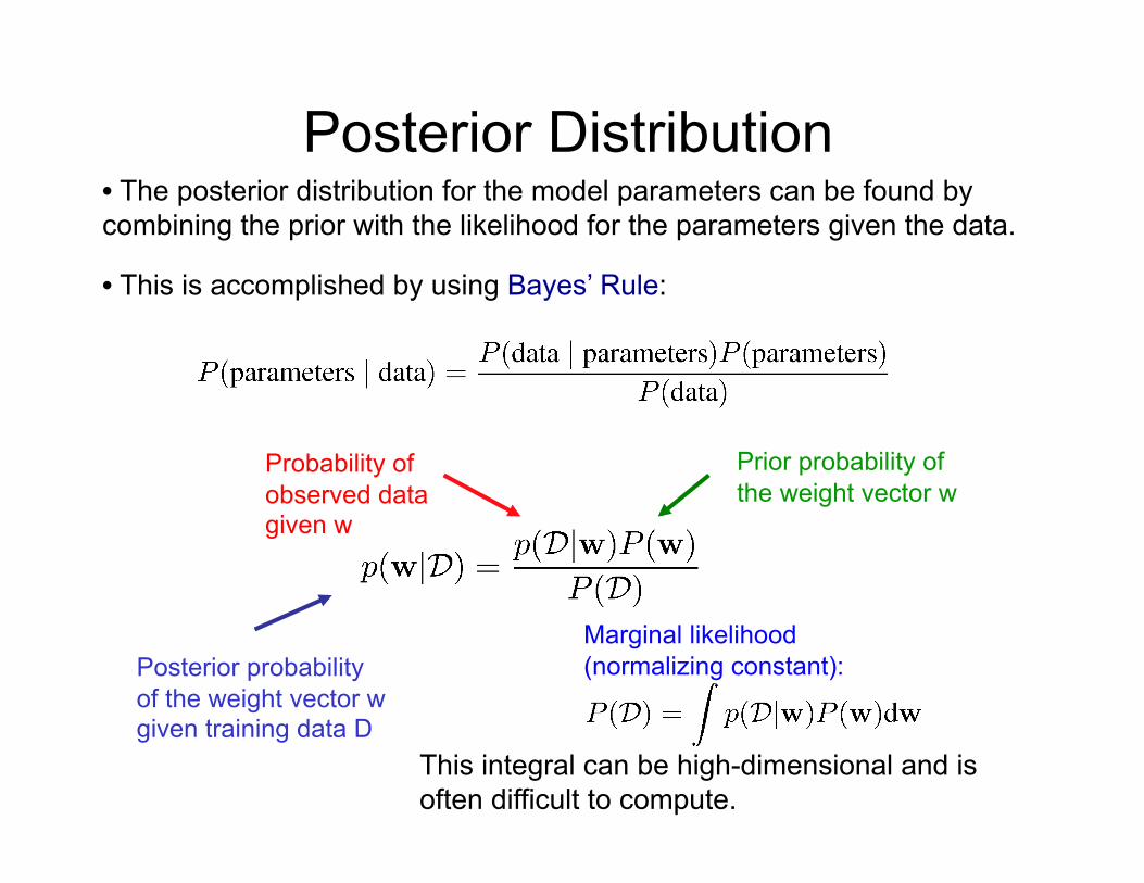
Posterior Distribution •  The posterior distribution for the model parameters can be found by combining the prior with the likelihood for the parameters given the data.

•  This is accomplished by using Bayes’ Rule:

Marginal likelihood (normalizing constant):

This integral can be high-dimensional and is often difficult to compute.

Posterior probability of the weight vector w given training data D

Probability of observed data given w

Prior probability of the weight vector w

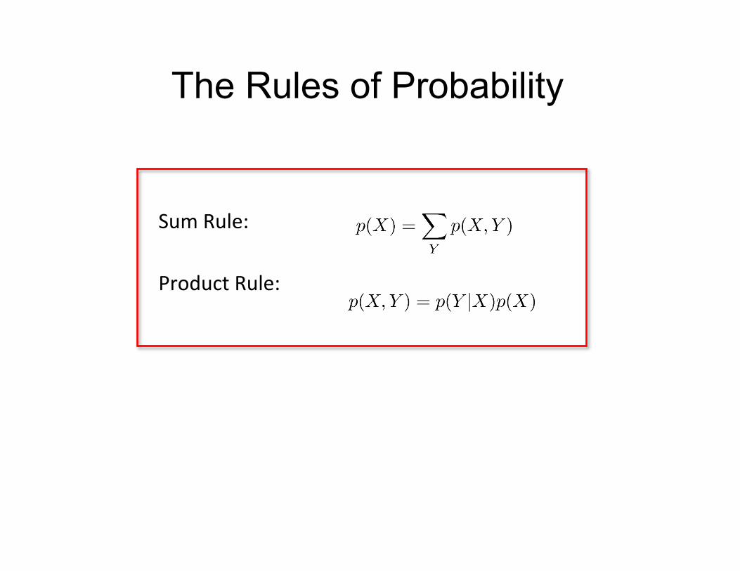
The Rules of Probability

Sum  Rule:  

Product  Rule:  

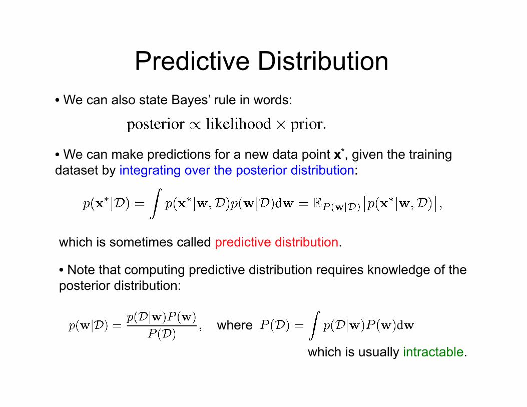
Predictive Distribution •  We can also state Bayes’ rule in words:

which is sometimes called predictive distribution.

•  Note that computing predictive distribution requires knowledge of the posterior distribution:

where

which is usually intractable.

•  We can make predictions for a new data point x*, given the training dataset by integrating over the posterior distribution:

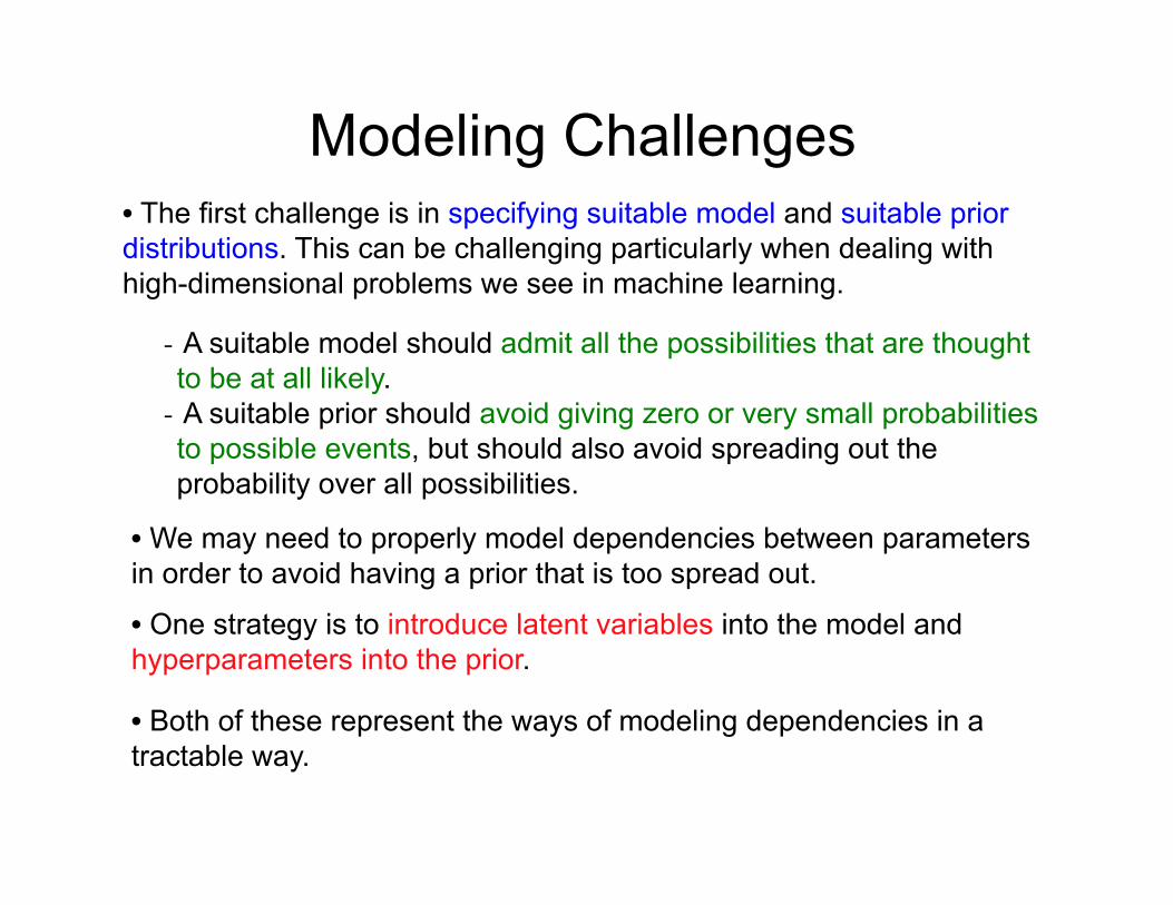
Modeling Challenges •  The first challenge is in specifying suitable model and suitable prior distributions. This can be challenging particularly when dealing with high-dimensional problems we see in machine learning.

•  We may need to properly model dependencies between parameters in order to avoid having a prior that is too spread out.

-  A suitable model should admit all the possibilities that are thought to be at all likely. -  A suitable prior should avoid giving zero or very small probabilities to possible events, but should also avoid spreading out the probability over all possibilities.

•  One strategy is to introduce latent variables into the model and hyperparameters into the prior.

•  Both of these represent the ways of modeling dependencies in a tractable way.

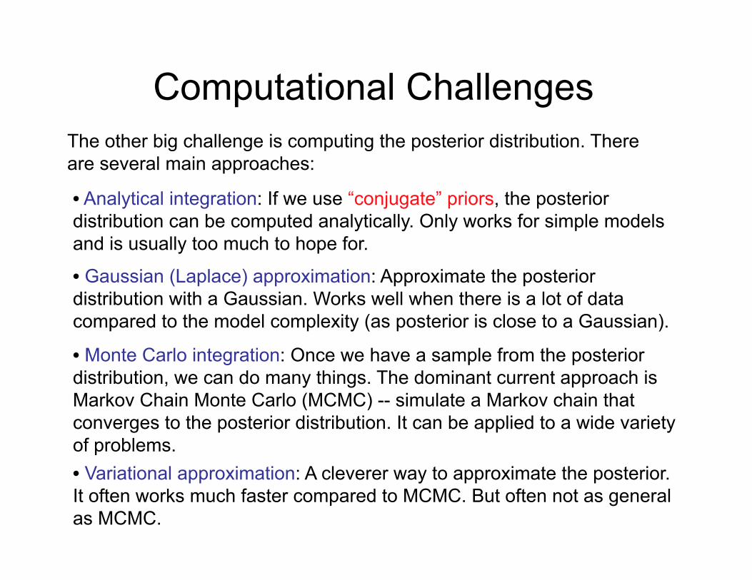
Computational Challenges The other big challenge is computing the posterior distribution. There are several main approaches:

•  Analytical integration: If we use “conjugate” priors, the posterior distribution can be computed analytically. Only works for simple models and is usually too much to hope for.

•  Gaussian (Laplace) approximation: Approximate the posterior distribution with a Gaussian. Works well when there is a lot of data compared to the model complexity (as posterior is close to a Gaussian).

•  Monte Carlo integration: Once we have a sample from the posterior distribution, we can do many things. The dominant current approach is Markov Chain Monte Carlo (MCMC) -- simulate a Markov chain that converges to the posterior distribution. It can be applied to a wide variety of problems. •  Variational approximation: A cleverer way to approximate the posterior. It often works much faster compared to MCMC. But often not as general as MCMC.

Bayesian Linear Regression •  Given observed inputs and corresponding target values we can write down the likelihood function:

where represent our basis functions.

•  The corresponding conjugate prior is given by a Gaussian distribution:

•  As both the likelihood and the prior terms are Gaussians, the posterior distribution will also be Gaussian.

•  If the posterior distributions p(θ|x) are in the same family as the prior probability distribution p(θ), the prior and posterior are then called conjugate distributions, and the prior is called a conjugate prior for the likelihood.

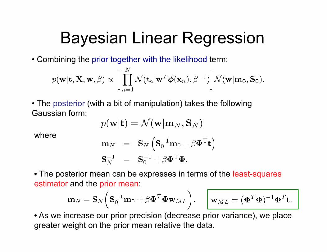
Bayesian Linear Regression •  Combining the prior together with the likelihood term:

•  The posterior (with a bit of manipulation) takes the following Gaussian form:

where

•  The posterior mean can be expresses in terms of the least-squares estimator and the prior mean:

•  As we increase our prior precision (decrease prior variance), we place greater weight on the prior mean relative the data.

Bayesian Linear Regression •  Consider a zero mean isotropic Gaussian prior, which is governed by a single precision parameter ®:

•  If we consider an infinitely broad prior, ® ! 0, the mean mN of the posterior distribution reduces to maximum likelihood value wML.

for which the posterior is Gaussian with:

•  The log of the posterior distribution is given by the sum of the log-likelihood and the log of the prior:

•  Maximizing this posterior with respect to w is equivalent to minimizing the sum-of-squares error function with a quadratic regulation term ¸ = ® / ¯.

Bayesian Linear Regression •  Consider a linear model of the form: •  The training data is generated from the function with by first choosing xn uniformly from [-1;1], evaluating and then adding a small Gaussian noise.

•  Goal: recover the values of from such data.

0 data points are observed: Prior   Data  Space  

Bayesian Linear Regression Prior   Data  Space  0 data points are observed:

1 data point is observed: Likelihood   Posterior   Data  Space  

Bayesian Linear Regression 0 data points are observed.

1 data point is observed.

2 data points are observed.

20 data points are observed.

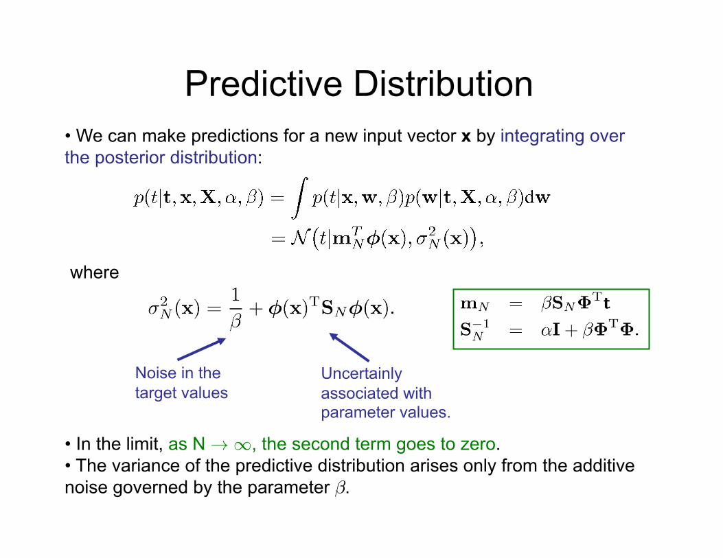
Predictive Distribution •  We can make predictions for a new input vector x by integrating over the posterior distribution:

where

•  In the limit, as N ! 1, the second term goes to zero. •  The variance of the predictive distribution arises only from the additive noise governed by the parameter ¯.

Noise in the target values

Uncertainly associated with parameter values.

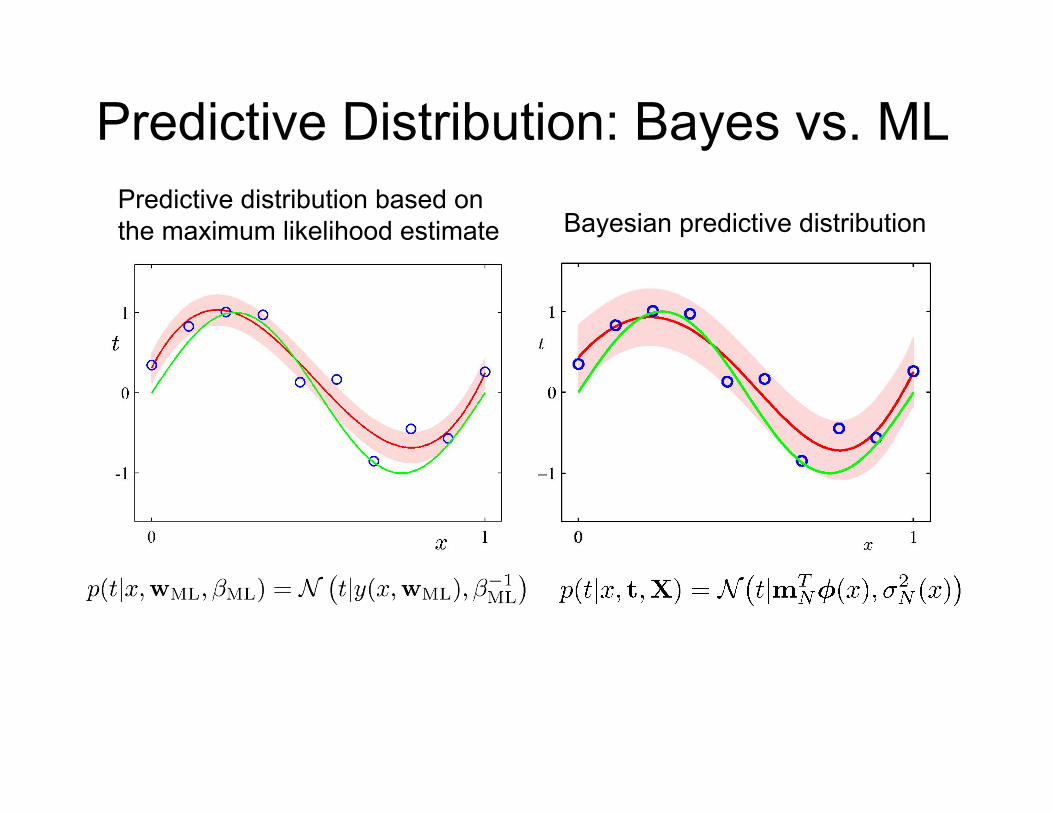
Predictive Distribution: Bayes vs. ML

Bayesian predictive distribution Predictive distribution based on the maximum likelihood estimate

Predictive Distribution Sinusoidal dataset, 9 Gaussian basis functions.

Predictive distribution Samples from the posterior

Predictive Distribution Sinusoidal dataset, 9 Gaussian basis functions.

Predictive distribution Samples from the posterior

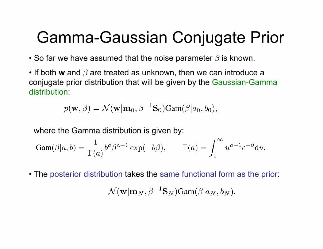
Gamma-Gaussian Conjugate Prior •  So far we have assumed that the noise parameter ¯ is known.

•  If both w and ¯ are treated as unknown, then we can introduce a conjugate prior distribution that will be given by the Gaussian-Gamma distribution:

where the Gamma distribution is given by:

•  The posterior distribution takes the same functional form as the prior:

Equivalent Kernel •  The predictive mean can be written as:

Equivalent  kernel  or  smoother  matrix.  

•  The mean of the predictive distribution at a time x can be written as a linear combination of the training set target values.

•  Such regression functions are called linear smoothers.

Equivalent Kernel

•  We can avoid the use of basis functions and define the kernel function directly, leading to Gaussian Processes.

•  The kernel as a covariance function:

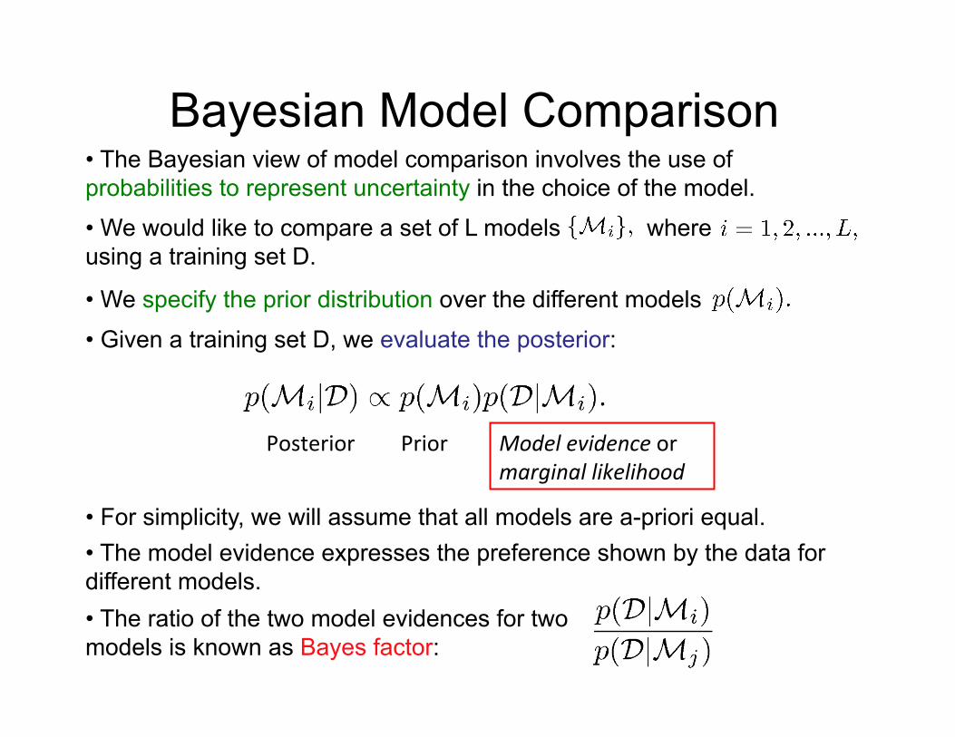
Bayesian Model Comparison •  The Bayesian view of model comparison involves the use of probabilities to represent uncertainty in the choice of the model.

•  We specify the prior distribution over the different models

•  Given a training set D, we evaluate the posterior:

Posterior   Prior   Model  evidence  or  marginal  likelihood  

•  The model evidence expresses the preference shown by the data for different models. •  The ratio of the two model evidences for two models is known as Bayes factor:

•  For simplicity, we will assume that all models are a-priori equal.

•  We would like to compare a set of L models where using a training set D.

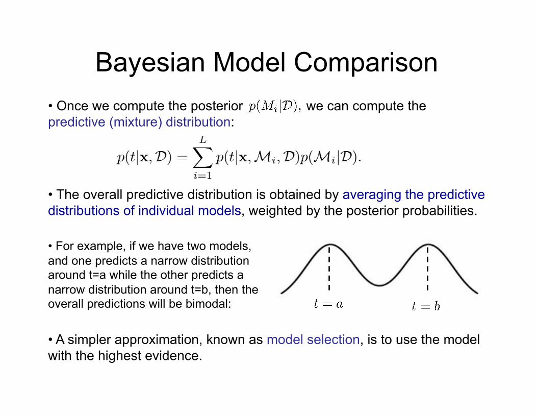
Bayesian Model Comparison •  Once we compute the posterior we can compute the predictive (mixture) distribution:

•  A simpler approximation, known as model selection, is to use the model with the highest evidence.

•  The overall predictive distribution is obtained by averaging the predictive distributions of individual models, weighted by the posterior probabilities.

•  For example, if we have two models, and one predicts a narrow distribution around t=a while the other predicts a narrow distribution around t=b, then the overall predictions will be bimodal:

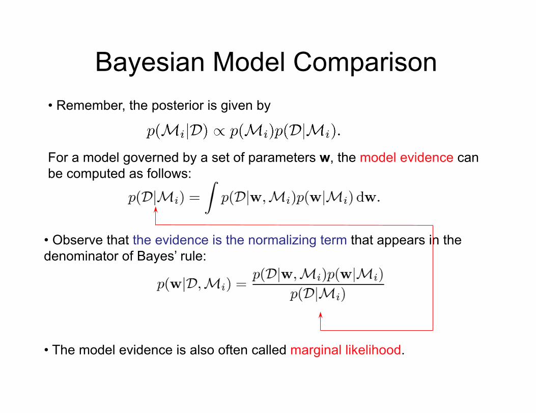
Bayesian Model Comparison •  Remember, the posterior is given by

For a model governed by a set of parameters w, the model evidence can be computed as follows:

•  The model evidence is also often called marginal likelihood.

•  Observe that the evidence is the normalizing term that appears in the denominator of Bayes’ rule:

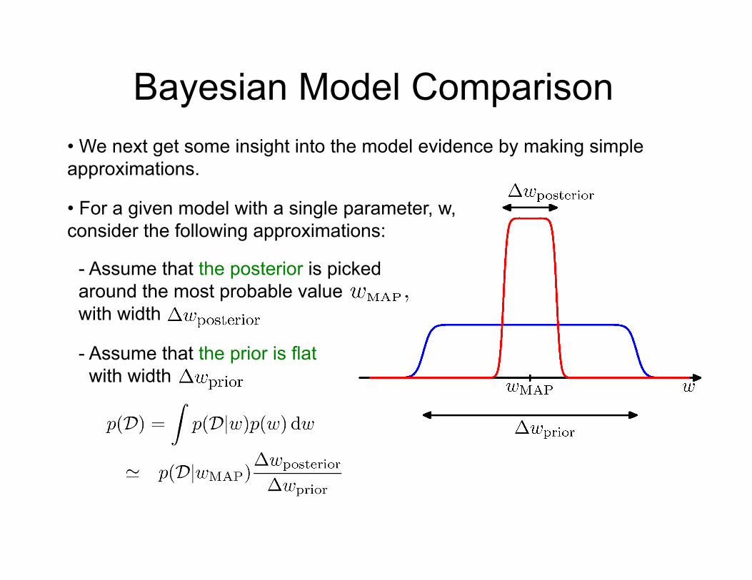
Bayesian Model Comparison •  We next get some insight into the model evidence by making simple approximations.

•  For a given model with a single parameter, w, consider the following approximations:

-  Assume that the prior is flat with width

-  Assume that the posterior is picked around the most probable value with width

Bayesian Model Comparison •  Taking the logarithms, we obtain:

NegaCve  

•  With M parameters, all assumed to have the same ratio:

NegaCve  and  linear  in  M.  

•  As we increase the complexity of the model (increase the number of adaptive parameters M), the first term will increase, whereas the second term will decrease due to the dependence on M. •  The optimal model complexity: trade-off between these two competing terms.

Bayesian Model Comparison

•  The simple model cannot fit the data well, whereas the more complex model spreads its predictive probability and so assigns relatively small probability to any one of them.

Matching data and model complexity

•  For the particular observed dataset the model with intermediate complexity has the largest evidence.

•  The marginal likelihood is very sensitive to the prior used! •  Computing the marginal likelihood makes sense only if you are certain about the choice of the prior.

Evidence Approximation

•  The fully Bayesian predictive distribution is then given by marginalizing over model parameters as well as hyperparameters:

•  However, this integral is intractable (even when everything is Gaussian). Need to approximate.

target and input on test case

precision of output noise

precision of the prior

training data: inputs and targets

Likelihood posterior over weights

posterior over hyperparameters

•  In the fully Bayesian approach, we would also specify a prior distribution over the hyperparameters

•  Note: the fully Bayesian approach is to integrate over the posterior distribution for This can be done by MCMC, which we will consider later. For now, we will use evidence approximation: much faster.

Evidence Approximation •  The fully Bayesian predictive distribution is given by:

•  If we assume that the posterior over hyperparameters ® and ¯ is sharply picked, we can approximate:

•  So we integrate out parameters but maximize over hyperparameters.

•  This is known as empirical Bayes, Type II Maximum Likelihood, Evidence Approximation.

where is the mode of the posterior

Evidence Approximation •  From Bayes’ rule we obtain:

•  If we assume that the prior over hyperparameters is flat, we get:

•  The values are obtained by maximizing the marginal likelihood

•  This will allow us to determine the values of these hyperparameters from the training data.

•  Recall that the ratio ®/¯ is analogous to the regularization parameter.

Evidence Approximation •  The marginal likelihood is obtained by integrating out parameters:

•  We can write the evidence function in the form:

where

•  Using standard results for the Gaussian distribution, we obtain:

Some Fits to the Data

For M=9, we have fitted the training data perfectly.

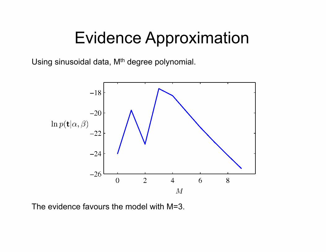
Evidence Approximation Using sinusoidal data, Mth degree polynomial.

The evidence favours the model with M=3.

Maximizing the Evidence

•  To maximize the evidence with respect to ® and ¯, define the following eigenvector equation:

•  Therefore the matrix:

has eigenvalues ® + ¸i.

Precision matrix of the Gaussian posterior distribution

•  The derivative:

•  Remember:

Maximizing the Evidence

where the quantity °, effective number of parameters, can be defined as:

•  Differentiating , the stationary points with respect to ® satisfy:

•  Remember:

where

•  Similarly:

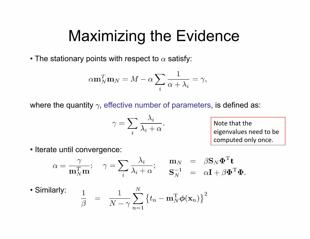
Maximizing the Evidence •  The stationary points with respect to ® satisfy:

where the quantity °, effective number of parameters, is defined as:

•  Iterate until convergence:

Note  that  the  eigenvalues  need  to  be  computed  only  once.  

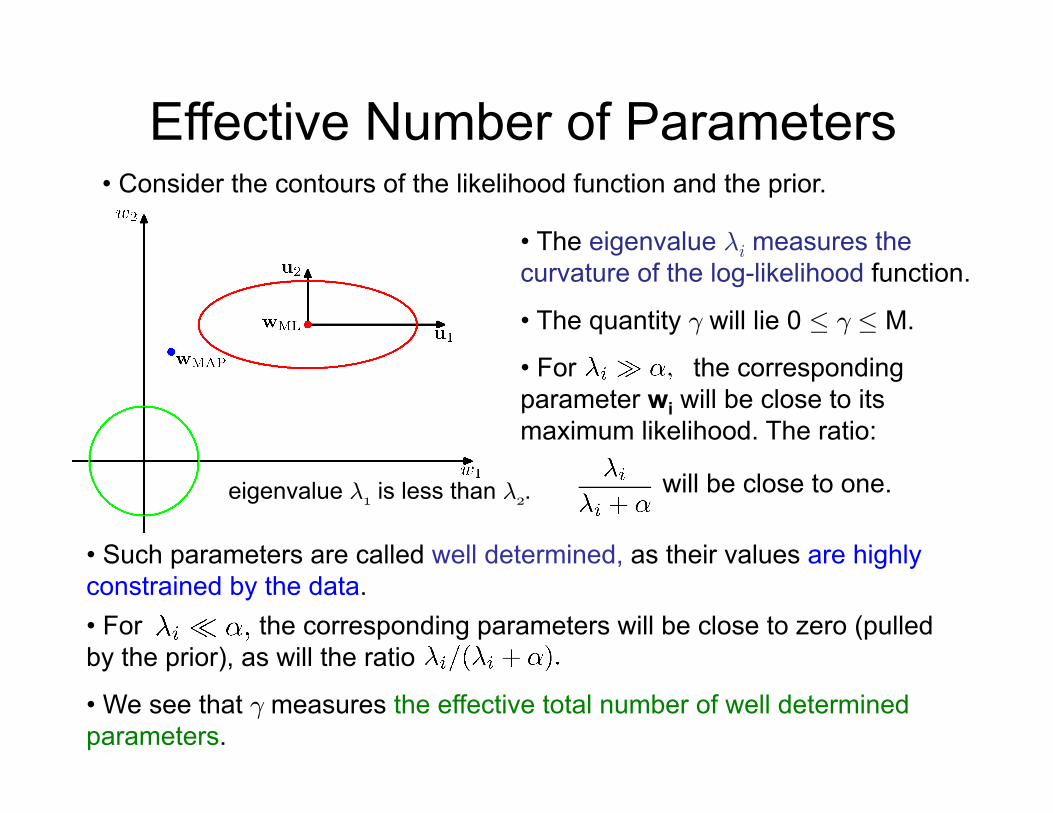
Effective Number of Parameters •  Consider the contours of the likelihood function and the prior.

eigenvalue ¸1 is less than ¸2.

•  The eigenvalue ¸i measures the curvature of the log-likelihood function.

•  The quantity ° will lie 0 · ° · M.

•  For the corresponding parameter wi will be close to its maximum likelihood. The ratio:

will be close to one.

•  Such parameters are called well determined, as their values are highly constrained by the data. •  For the corresponding parameters will be close to zero (pulled by the prior), as will the ratio

•  We see that ° measures the effective total number of well determined parameters.

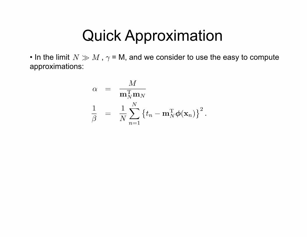
•  In the limit , ° = M, and we consider to use the easy to compute approximations:

Quick Approximation

Limitations •  M basis function along each dimension of a D-dimensional input space requires MD basis functions: the curse of dimensionality.

•  Fortunately, we can get away with fewer basis functions, by choosing these using the training data (e.g. adaptive basis functions), which we will see later.

•  Second, the data vectors typically lie close to a nonlinear low-dimensional manifold, whose intrinsic dimensionality is smaller than that of the input space.