SST Analysis in NCEP GFS

Xu Li, John DerberEMC/NCEP

General Picture --- SST Improvement

Extract SST information from satellite data more effectively

From Empirical retrievalto Physical retrieval

to Direct assimilation of radiances

Better SST Analysis Product

Resolve the vertical structure from surface to diurnal warming depth

Enable to use depth dependent observations consistently

Require to solve new, related issues

Assimilation scheme• SST is analyzed with the atmospheric data

assimilation system (GSI) in NCEP GFS– Add a new analysis variable (SST or equivalent) to GSI

• Single cost function with more elements in the state vector– Add observation data related to SST– Error variance and correlation length for the new analysis variable

• Problems– SST prediction– Observation operators (H) for the new analysis variable (x) are

not available, if the observations (y) are depth dependent.– Jacobi of the new observation operators need to be derived– Different lower temperature condition required for atmospheric

model (Ts) and radiative transfer model (Tr).

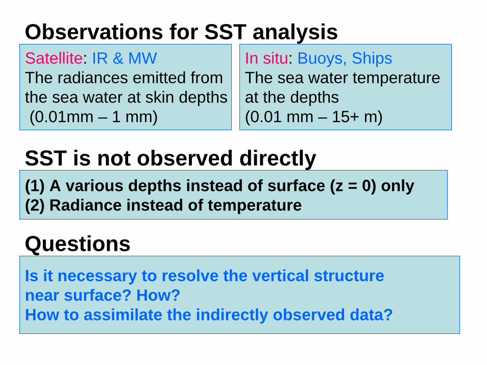
Observations for SST analysisSatellite: IR & MWThe radiances emitted from the sea water at skin depths(0.01mm – 1 mm)

In situ: Buoys, ShipsThe sea water temperature at the depths (0.01 mm – 15+ m)

(1) A various depths instead of surface (z = 0) only(2) Radiance instead of temperature

SST is not observed directly

QuestionsIs it necessary to resolve the vertical structure near surface? How?How to assimilate the indirectly observed data?

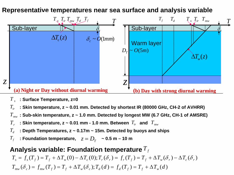
(a) Night or Day without diurnal warming (b) Day with strong diurnal warming

Representative temperatures near sea surface and analysis variable

skinT

fT

z

sT irT mwTdT

Warm layer

Sub-layerSub-layer

z

TT

)(zTwΔ

fTsT irT mwT dT

)1(~ mmOcδ

)5(~ mODT

fT

sT

irT

mwT

dT: Foundation temperature, ~ 0.5 m – 10 mTDz

: Surface Temperature, z=0

: Depth Temperatures, z ~ 0.17m ~ 15m. Detected by buoys and ships

=

: Skin temperature, z ~ 0.01 mm. Detected by shortest IR (80000 GHz, CH-2 of AVHRR) : Sub-skin temperature, z ~ 1.0 mm. Detected by longest MW (6.7 GHz, CH-1 of AMSRE)

rT : Skin temperature, z ~ 0.01 mm - 1.0 mm. Between and irT mwT

Analysis variable: Foundation temperature fT

cδcδ

)(zTcΔ

)()()();()()(

)()()()();0()0()(

dTTTfdTTTTfT

TTTTfTTTTTfT

wffddcwffmwcmw

rcrwffrrrcwffss

Δ+==Δ+==

Δ−Δ+==Δ−Δ+==

δδ

δδδ

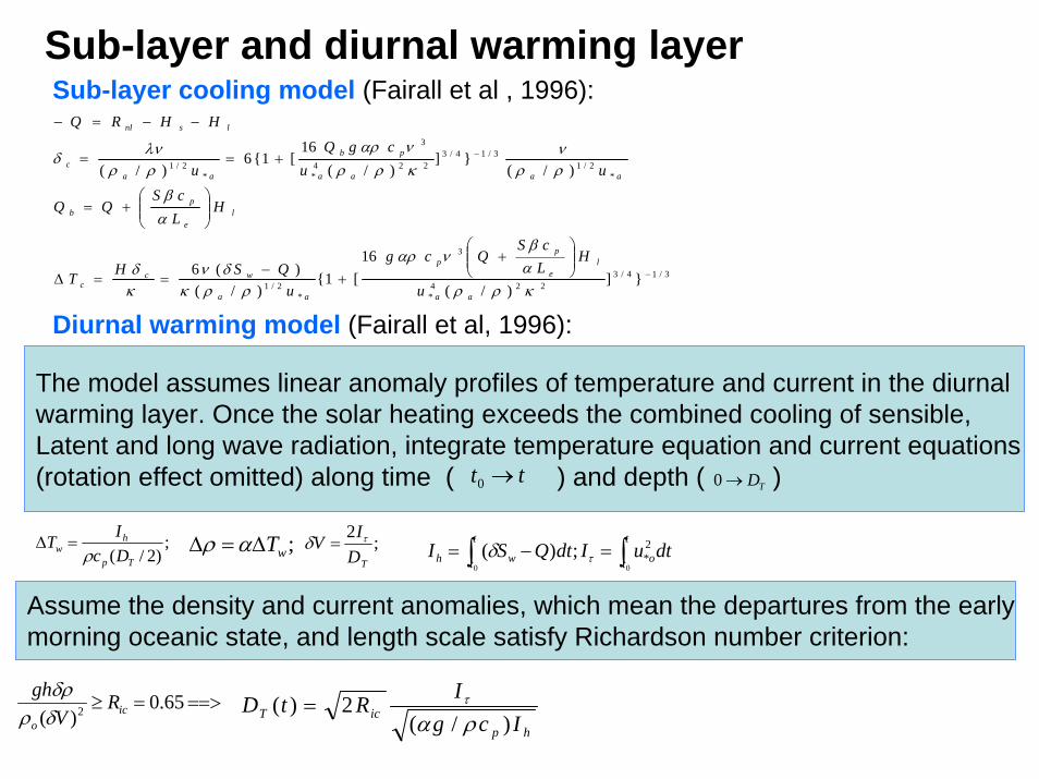
Sub-layer and diurnal warming layer

TD

;)2/( Tp

hw Dc

ITρ

=Δ

Diurnal warming model (Fairall et al, 1996):

3/14/3224

*

3

*2/1

*2/1

3/14/3224

*

3

*2/1

}])/(

16[1{

)/()(6

)/(}]

)/(16

[1{6)/(

−

−

⎟⎟⎠

⎞⎜⎜⎝

⎛+

+−

==Δ

⎟⎟⎠

⎞⎜⎜⎝

⎛+=

+==

−−=−

κρραβ

ναρ

ρρκδν

κδ

αβ

ρρν

κρρναρ

ρρλνδ

aa

le

pp

aa

wcc

le

pb

aaaa

pb

aac

lsnl

u

HLcS

Qcg

uQSHT

HLcS

QQ

uucgQ

u

HHRQ

Sub-layer cooling model (Fairall et al , 1996):

hpicT Icg

IRtD)/(

2)(ρατ=

The model assumes linear anomaly profiles of temperature and current in the diurnal warming layer. Once the solar heating exceeds the combined cooling of sensible, Latent and long wave radiation, integrate temperature equation and current equations(rotation effect omitted) along time ( ) and depth ( )

;2

TDIV τδ =;wTΔ=Δ αρ

Assume the density and current anomalies, which mean the departures from the earlymorning oceanic state, and length scale satisfy Richardson number criterion:

==>=≥ 65.0)( 2 ic

o

RV

ghδρδρ

tt →0 TD→0

∫∫ =−=t

t o

t

t wh dtuIdtQSI00

2*;)( τδ

)()()( dTTTfdT wffdd Δ+==

dfdc

ffc

TTfH

TTH

=>

=>

)]([

)(

)()()()( rcrwffrrr TTTTfT δδδ Δ−Δ+==

Conversion between SST ( ) and :

Observation operators from to and :

sfscffc TTfHTTH =>=> )]([;)(

Sensitivities of the representative temperatures to :

)0()0()( cwffss TTTTfT Δ−Δ+==

rfrr

rrr

TTfHTTH=>

=>)]([

)(

Satellite data :

sT rT

Conventional data :fT

Conventional data:

),,(0)](,,[

0)]},(([,,{)()()(

d

mw

mw

s

s

wd

f

dswfdd

sThTwfddwffdd

TT

TT

TTP

TTTTTTF

TDIDTTTFdTTTfdT

∂∂

∂∂

∂Δ∂

=∂∂

==>=Δ

=Δ==>Δ+==

Satellite data:

),(

0)]()(,,[

)()()()(

r

s

s

wr

f

r

scswfrr

rcrwffrrr

TT

TTP

TT

TTTTTTF

TTTTfT

∂∂

∂Δ∂

=∂∂

=>

=Δ−Δ=>

Δ−Δ+== δδδ

fT dT rT

f

d

TT∂∂

f

r

TT

∂∂

Observation operator: To transform analysis variable to corresponding partner in observationspace.

: available, interpolation operator: available, radiative transfer model

cH

rH

: Implicit compound function to relate and through

Heat fluxes and therefore )( dzTd =

fTsT

dF

)0( =Δ zTw

TD

)/( 0ttI −τ

)/( 0ttIh −

Diurnal warming model run with 3-hourly GFS fluxes

)0( =Δ zTc

cδ

Sub-layer model run with 3-hourly GFS fluxes

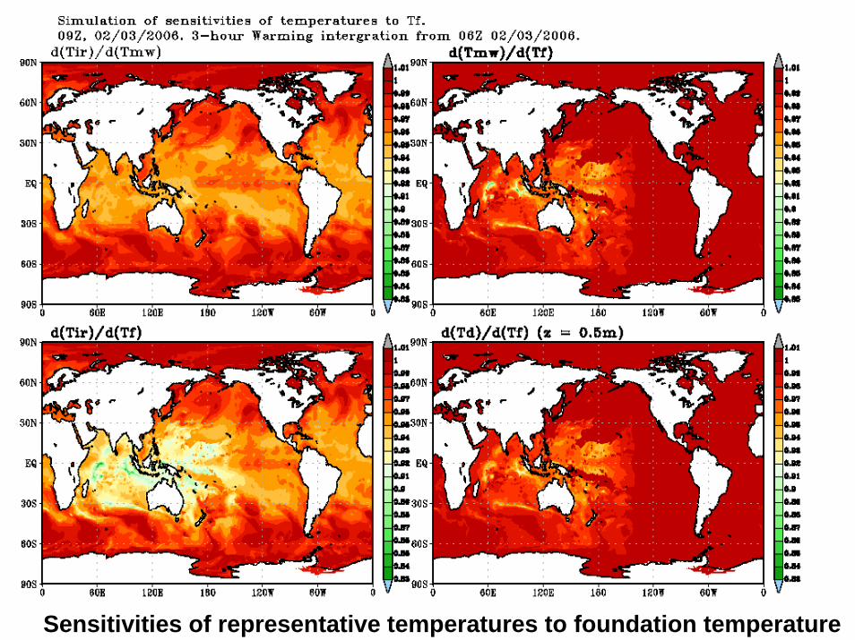
Sensitivities of representative temperatures to foundation temperature

)0( =Δ zTw cw TT Δ−Δ

cTΔ

Experiment:Use the SST currently used by GFS, as the foundation temperature. Satellite instruments are divided into IR and MW:For IR:

For MW: Then, 7-day analysis is done with GSI, GFS forecast (03, 06, 09) used as the first guess; GFS fluxes used to get and

Control Run:

)0()0( =Δ−=Δ+= zTzTTT cwctlir

)0( =Δ+= zTTT wctlmw

ctlmwir TTT ==

ctlT

wTΔ cTΔ

Impacts of sea water diurnal warming and sub-layer cooling on AVHRR radiance simulation (Bias), based on the data used in both experiments

)0()0( =Δ−=Δ zTzT cwBias of Ctl RunBias of Exp.

Number of used data in Ctl RunNumber of used data in Exp.

Difference of the number of used data in two runs: (Exp – Ctl)

Bias of Exp. ABias of Exp. B

Number of used data in Exp. ANumber of used data in Exp. B

Difference of the number of used data in two Exps: (A – B)

)0()0( =Δ−=Δ zTzT cw

Impacts of sea water diurnal warming and sub-layer cooling on the analysis of AVHRR data

+546

Plan

• Foundation temperature analysis in GSI– error statistics based on a period of analysis sample– How often the fluxes and therefore the diurnal

warming amount updated? – Parallel run

• Consistency among SST, fluxes and atmosphere

• Diurnal warming model improvement– Theoretical analysis done: rotation effect, vanish wind

handle, E-P effect, linear to exponent profile– Solar radiation penetration

• One-dimensional oceanic model– forecasting

fT

fT