Embed Size (px)
Citation preview
KR0100806
KAERI/TR-1619/2000
SSC-K ^ i > 3 H 4-§-*> * 1 ^ (Rev.O)
SSC-K Code User's Manual (Rev.O)
2000. 7
?>

PLEASE BE AWARE THATALL OF THE MISSING PAGES IN THIS DOCUMENT
WERE ORIGINALLY BLANK

2000
SSC-K ^ ^ 2 5 *Y%-7\- *]%*\ (Rev.O)
SSC-K Code User's Manual (Rev.O)
2000. 7

JBL
(KAERI)^ PoolU KALIMER £\ t
SSC-K (Supper System Code
ofKAERI)!- . SSC-K^ * ] ^ BNL °1H
SSC-L -I: 7ly}AS. £}<*) KALIMER
5 1 ^ 4 . ^ ^ SSC-K 2 £ ^ ^ H ^ 4
SSC-K ^ 4
fe SSC-K
ul
2 ^ 4 3
4 ^Hl^ SSC-L S =
(IHX) 2.
SSC-Kfe 71^5]
. 5
KALIMER>^§}4. 6
PSDRS 3L^ 7]^"S:>^4. 7 3M|fe
^-o.S. 8 3 N f e SSC-K
SSC-K ofl A>-8-€ Subroutines
SSC-K S ^ ^ l ^ l ^ ^
SSC-K
KALIMERssc-K
. SSC-K 3
SUMMARY
The Supper System Code of KAERI (SSC-K) is a best-estimate! system code for analyzing
a variety of off-normal or accidents in the heat transport system of a pool type LMR design. It is
being developed at Korea Atomic Energy Research Inititution (KAERI) on the basis of SSC-L,
originally developed at BNL to analyze loop-type LMR transients:. SSC-K can handle both
designs of loop and pool type LMRs. SSC-K contains detailed mechanistic models of transient
thermal, hydraulic, neutronic, and mechanical phenomena to describe the response of the reactor
core, icoolant, fuel elements, and structures to accident conditions.
This report provides an overview of recent model developments of the SSC-K computer
code, focusing on phenomenological model descriptions for new thermal, hydraulic, neutronic,
and mechnaical modules. A comprehensive description of the models for pool-type reactor is
given in Chapters 2 and 3; the steady-state plant characterization., prior to the initiation of
transient is described in Chapter 2 and their transient counterparts are: discussed in Chapter 3. In
Chapter 4, a discussion on the intermediate heat exchanger (IHX) is presented. The IHX model
of SSC-K is similar to that used in the SSC-L, except for some changes required for the pool-
type configuration of reactor vessel. In Chapter 5, an electromagnetic (EM) pump is modeled as
a component. There are two pump choices available in SSC-K; a centrifugal pump which was
originally imbedded into the SSC-L, and an EM pump which was introduced for the KALIMER
design. In Chapter 6, a model of passive safety decay heat removal system (PSDRS) is discussed,
which removes decay heat through the reactor and containment vessel walls to the ambient air
heat sink. In Chapter 7, models for various reactivity feedback effects are discussed. Reactivity
effects of importance in fast reactor include the Doppler effect, effects of sodium density changes,
effects of dimensional changes in core geometry. Finally in Chapter 8, constitutive laws and
correlations required to execute the SSC-K are described.
Test runs for typical LMFBR accident analyses have been performed for the qualitative
verification of the developed SSC-K modules. The analysis results will be issued as a separate
report. It was found that the present version of SSC-K would be used for the priliminary safety
analysis of KALIMER. However, the further validation of SSC-K is required for real
applications. It is noted that the user's manual of SSC-K will be revised later with the further
development of SSC-K code.
in

Table of Contents
• • - i i
Summary iii
Table of Contents iv
List of Figures viii
List of Tables x
1. INTRODUCTION 1-1
2. STEADY-STATE MODELS 2-1
2.1 Global Heat Balance 2-1
2.1.1 Steady State Calculation in IHX 2-2
2.2 Hot Pool Pressure Distribution 2-7
2.3 Thermal-Hydraulics for Fuel Assembly Region 2-8
2.3.1 Core Thermal-Hydraulics 2-8
2.3.2 Core Pressure Distribution 2-9
2.3.3 Upper Plenum Thermal-Hydraulics 2-14
2.3.4 Core Outlet Module Hydraulics 2-16
2.4 Loop Hydraulics 2-17
2.4.1 Hydraulics for IHX 2-17
2.4.2 Hydraulics for Pipes 2-18
2.4.3 Pump 2-19
2.4.4 Pressure Distribution of Pipes 2-20
2.4.5 Cold Pool Hydraulics 2-21
3. TRNSIENT MODELS 3-1
3.1 Flow Equations 3-1
3.1.1 Intact System 3-1
3.1.2 Damaged System 3-2
3.2 Pump Suction Pressure 3-3
3.3 Liquid Levels in Pools 3-4
3.4 Reactor Internal Pressure 3-6
3.4.1 Intact System 3-6
3.4.2 Damaged System 3-8
IV
3.5 Energy Balance in Hot Pool • 3-10
3.5.1 Lower Mixing Zone B: 3-11
3.5.2 Upper Mixing Zone A: 3-13
3.5.3 Other Temperatures in Hot Pool 3-14
3.6 Energy Balance in Cold Pool 3-15
4. INTERMEDIATE HEAT EXCHANGER 4-1
4.1 Pool Type IHX 4-1
4.2 Heat Transfer Model 4-2
4.3 Pressure Losses Model 4-6
4.4 Liquid Levels in Pools 4-8
5. ELECTROMAGNETIC PUMP 5-1
5.1 Pump Models • • 5-1
5.2 Correlations to Pump Data 5-4
6. PASSIVE DECAY HEAT REMOVAL SYSTE 6-1
6.1 Introduction 6-1
6.2 PSDRS Modeling 6-1
6.2.1 Basic Assumptions 6-1
6.2.2 Governing Equations 6-2
6.2.3 Solution Method 6-8
6.3 PSDRS Program 6-9
7. REACTIVITY MODELS 7-1
7.1 INTRODUCTION 7-1
7.2 Reactor Kinetics 7-2
7.2.1 Point Kinetics Equations 7-2
7.2.2 Prompt Jump Approximation 7-4
7.2.3 Kaganove Method 7-5
7.3 Reactivity Effects 7-7
7.3.1 Doppler Effect 7-8
7.3.1.1 Hard Spectrum Case 7-9
7.3.1.2 Soft Spectrum Case 7-11
7.3.1.3 Other Models •'• 7-13
7.3.2 Sodium Density Effect 7-14
7.3.3 Axial Expansion Effect 7-15
7.3.3.1 Free Fuel Expansion Model 7-18
7.3.3.2 Force Balance Controlled Expansion Model 7-20
7.3.3.3 Other Models 7-22
7.3.4 Radial Expansion Effect 7-23
7.3.4.1 SSC-KModel ; 7-23
7.3.4.2 Other Models 7-25
7.3.5 Control Rod Driveline Expansion Effect 7-27
7.4 Input Requirements for Reactivity Feedback Models 7-30
7.4.1 Doppler Effect 7-30
7.4.2 Sodium Density Effect 7-32
7.4.3 Axial Expansion Effect 7-33
7.4.4 Radial Expansion Effect 7-34
7.4.5 Control Rod Driveline Expansion Effect 7-35
7.5 Flowcharts 7-36
7.6 GEM Model 7-36
7.6.1 Current GEM Model 7-36
7.6.2 GEM Model Improvement 7-38
8. CONSTITUTIVE LAWS AND CORRELATIONS 8-1
8.1 Constitutive Laws 8-1
8.1.1 SSC-L Properties 8-1
8.1.1.1 Core and Blanket Fuel 8-1
8.1.1.2. Cladding and Structural Materials 8-5
8.1.2 Constitutive Laws for SSC-K 8-6
8.1.2.1 Metal Fuel Properties 8-6
8.1.2.2 Limitations and Future Work 8-12
8.1.3 Control Rod Material 8-12
8.1.4 Sodium 8-13
8.1.5 Water and Steam 8-19
8.2 Correlations 8-28
8.2.1 Friction Factor Correlations 8-28
8.2.1.1 Pressure Drop in Pipe • 8-28
8.2.1.2 Pressure Drop in Wire-Wrapped Rod Bundles 8-33
8.2.2 Heat Transfer Correlations 8-37
9. TWO-DIMENSIONAL HOT POOL MODEL 9-1
9.1 Introduction 9-1
VI

9.2 Theory 9-1
9.2.1 Governing Equations 9-1
9.2.2 Discretization of Governing Equation 9-3
9.2.3 Momentum Interpolation Method > • 9-3
9.2.4 Solution Algorithm 9-5
9.2.5 Treatment of Boundary Conditions 9-6
9.3 Modeling 9-7
9.4 Sample Run 9-8
9.4.1 Constant Inlet Temperature Increase 9-8
9.4.2 Unprotected Transient Overpower Events 9-9
REFERENCES 10-1
Appendix A SSC-K INPUT DESCRIPTION • A-l
Appendix B SUBROUTINES IN SSC-K B-l
vn
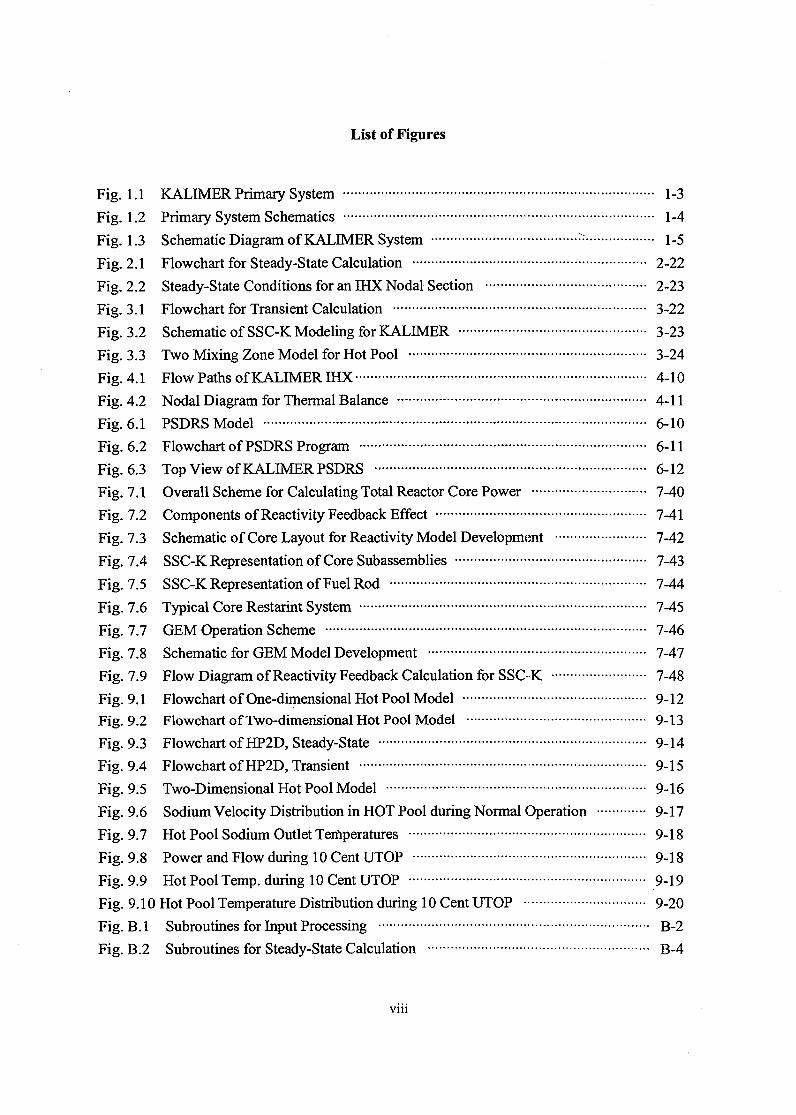
List of Figures
Fig. 1.1 KALIMER Primary System 1-3
Fig. 1.2 Primary System Schematics 1-4
Fig. 1.3 Schematic Diagram of KALIMER System - 1-5
Fig. 2.1 Flowchart for Steady-State Calculation 2-22
Fig. 2.2 Steady-State Conditions for an IHX Nodal Section 2-23
Fig. 3.1 Flowchart for Transient Calculation 3-22
Fig. 3.2 Schematic of SSC-K Modeling for KALIMER 3-23
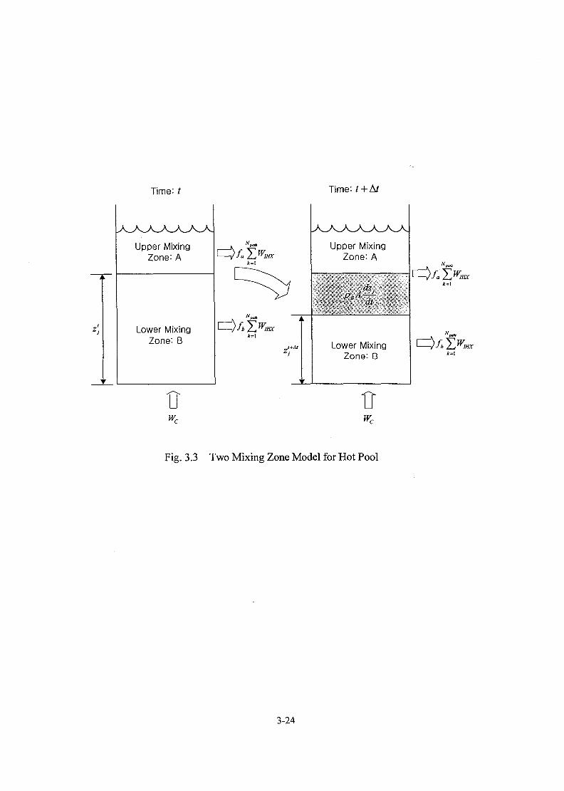
Fig. 3.3 Two Mixing Zone Model for Hot Pool 3-24
Fig. 4.1 Flow Paths of KALIMER IHX 4-10
Fig. 4.2 Nodal Diagram for Thermal Balance 4-11
Fig. 6.1 PSDRS Model 6-10
Fig. 6.2 Flowchart of PSDRS Program 6-11
Fig. 6.3 Top View of KALIMER PSDRS 6-12
Fig. 7.1 Overall Scheme for Calculating Total Reactor Core Power 7-40
Fig. 7.2 Components of Reactivity Feedback Effect 7-41
Fig. 7.3 Schematic of Core Layout for Reactivity Model Development 7-42
Fig. 7.4 SSC-K Representation of Core Subassemblies 7-43
Fig. 7.5 SSC-K Representation of Fuel Rod 7-44
Fig. 7.6 Typical Core Restarint System 7-45
Fig. 7.7 GEM Operation Scheme 7-46
Fig. 7.8 Schematic for GEM Model Development 7-47
Fig. 7.9 Flow Diagram of Reactivity Feedback Calculation for SSC-K 7-48
Fig. 9.1 Flowchart of One-dimensional Hot Pool Model 9-12
Fig. 9.2 Flowchart of Two-dimensional Hot Pool Model 9-13
Fig. 9.3 Flowchart of HP2D, Steady-State 9-14
Fig. 9.4 Flowchart of HP2D, Transient 9-15
Fig. 9.5 Two-Dimensional Hot Pool Model 9-16
Fig. 9.6 Sodium Velocity Distribution in HOT Pool during Normal Operation 9-17
Fig. 9.7 Hot Pool Sodium Outlet Temperatures 9-18
Fig. 9.8 Power and Flow during 10 Cent UTOP 9-18
Fig. 9.9 Hot Pool Temp, during 10 Cent UTOP 9-19
Fig. 9.10 Hot Pool Temperature Distribution during 10 Cent UTOP 9-20
Fig. B.I Subroutines for Input Processing B-2
Fig. B.2 Subroutines for Steady-State Calculation B-4
Vll l

Fig. B.3 Subroutines for Transient Calculation B-8
Fig. B.4 Subroutines for Steam Generator (MINET Portion) B-17
Fig. B.5 All Subroutines Employed into SSC-K B-21
IX

List of Tables
Table 3-1 Code Modification List 3-19
Table 5-1 Correlation Coefficients for Use with the LMR Pumps 5-4
Table 8-1 Parameters on Fuel Thermal Conductivity and Specific Heat Correlations 8-2
Table 8-2 Parameters in Fuel Coefficient of Thermal Expansion, Density and Emissivity
Correlations • 8-4
Table 8-3 Parameters for Cladding and Structural Material Properties 8-6
Table 8-4 Parameters for Control Rod Material Properties 8-14
Table 8-5 Values of Coefficients for Temperature of Compressed Liquid Water 8-22
Table 8-6 Values of Coefficients for Temperature of Compressed Water Vapor 8-22
Table 8-7 Values of Coefficients for Density of Compressed Liquid Water 8-22
Table 8-8 Values of Coefficients for Viscosity of Compressed Liquid Water 8-25
Table 8-9 Values of Coefficients for Viscosity of Superheated Water Vapor 8-26
Table 8-10 Roughness various piping materials 8-29
Table 8-11 FormLoss Coefficient for Various Flow Restrictions 8-32
Table 8-12 Values of Constants in Equation^8-92) 8-34
Table 8-13 Important Parameters ofCRBR Hexagonal Assemblies 8-35
Table 8-14 Comparsion of correlations used for SSC-L and SSC-K 8-40
Table 9-1 Initial and Key Operating Parameters 9-11
1. INTRODUCTION
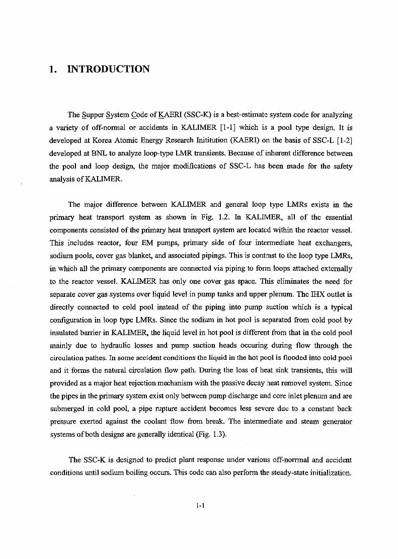
The Supper System Code of KAERI (SSC-K) is a best-estimate system code for analyzing
a variety of off-normal or accidents in KALIMER [1-1] which 1:3 a pool type design. It is
developed at Korea Atomic Energy Research Inititution (KAERI) on the basis of SSC-L [1-2]
developed at BNL to analyze loop-type LMR transients. Because of inherent difference between
the pool and loop design, the major modifications of SSC-L has been made for the safety
analysis of KALIMER.
The major difference between KALIMER and general loop type LMRs exists in the
primary heat transport system as shown in Fig. 1.2. In KALIMER, all of the essential
components consisted of the primary heat transport system are located within the reactor vessel.
This includes reactor, four EM pumps, primary side of four intermediate heat exchangers,
sodium pools, coyer gas blanket, and associated pipings. This is contrast to the loop type LMRs,
in which all the primary components are connected via piping to form loops attached externally
to the reactor vessel. KALIMER has only one cover gas space. Tins eliminates the need for
separate cover gas systems over liquid level in pump tanks and upper plenum. The IHX outlet is
directly connected to cold pool instead of the piping into pump suction which is a typical
configuration in loop type LMRs. Since the sodium in hot pool is separated from cold pool by
insulated barrier in KALIMER, the liquid level in hot pool is different from that in the cold pool
mainly due to hydraulic losses and pump suction heads occuring during flow through the
circulation pathes. In some accident conditions the liquid in the hot pool is flooded into cold pool
and it forms the natural circulation flow path. During the loss of heat sink transients, this will
provided as a major heat rejection mechanism with the passive decay heat removel system. Since
the pipes in the primary system exist only between pump discharge and core inlet plenum and are
submerged in cold pool, a pipe rupture accident becomes less severe due to a constant back
pressure exerted against the coolant flow from break. The intermediate and steam generator
systems of both designs are generally identical (Fig. 1.3).
The SSC-K is designed to predict plant response under various off-norrmal and accident
conditions until sodium boiling occurs. This code can also perform the steady-state initialization.
1-1
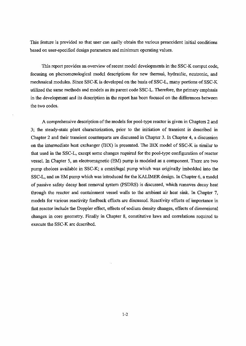
This feature is provided so that user can easily obtain the various preaccident initial conditions
based on user-specified design parameters and minimum operating values.
This report provides an overview of recent model developments in the SSC-K comput code,
focusing on phenomenological model descriptions for new thermal, hydraulic, neutronic, and
mechnaical modules. Since SSC-K is developed on the basis of SSC-L, many portions of SSC-K
utilized the same methods and models as its parent code SSC-L. Therefore, the primary emphasis
in the development and its description in the report has been focused on the differences between
the two codes.
A comprehensive description of the models for pool-type reactor is given in Chapters 2 and
3; the steady-state plant characterization, prior to the initiation of transient is described in
Chapter 2 and their transient counterparts are discussed in Chapter 3. In Chapter 4, a discussion
on the intermediate heat exchanger (IHX) is presented. The IHX model of SSC-K is similar to
that used in the SSC-L, except some changes required for the pool-type configuration of reactor
vessel. In Chapter 5, an electromagnetic (EM) pump is modeled as a component. There are two
pump choices available in SSC-K; a centrifugal pump which was originally imbedded into the
SSC-L, and an EM pump which was introduced for the KALIMER design. In Chapter 6, a model
of passive safety decay heat removal system (PSDRS) is discussed, which removes decay heat
through the reactor and containment vessel walls to the ambient air heat sink. In Chapter 7,
models for various reactivity feedback effects are discussed. Reactivity effects of importance in
fast reactor include the Doppler effect, effects of sodium density changes, effects of dimensional
changes in core geometry. Finally in Chapter 8, constitutive laws and correlations required to
execute the SSC-K are described.
1-2

Z6VSTP • -
Z6UPTLZ6UPLN - A-
Z60N0Z
Z6NALV
Z6TC0R J
Z6BC0RZ6IN0Z
Z6REF
Fig. 1.1 KALIMER Primary System
1-3

FromlHX
OUTLET PLENUM
TTTCORE
INLET PLENUM
PUMP
To Reactor
IHX
(a) Loop-type LMR
(b)Pool-type LMR
Fig. 1.2 Primary System Schematics
1-4

3TO'
STEAMGENERATOR
EMP
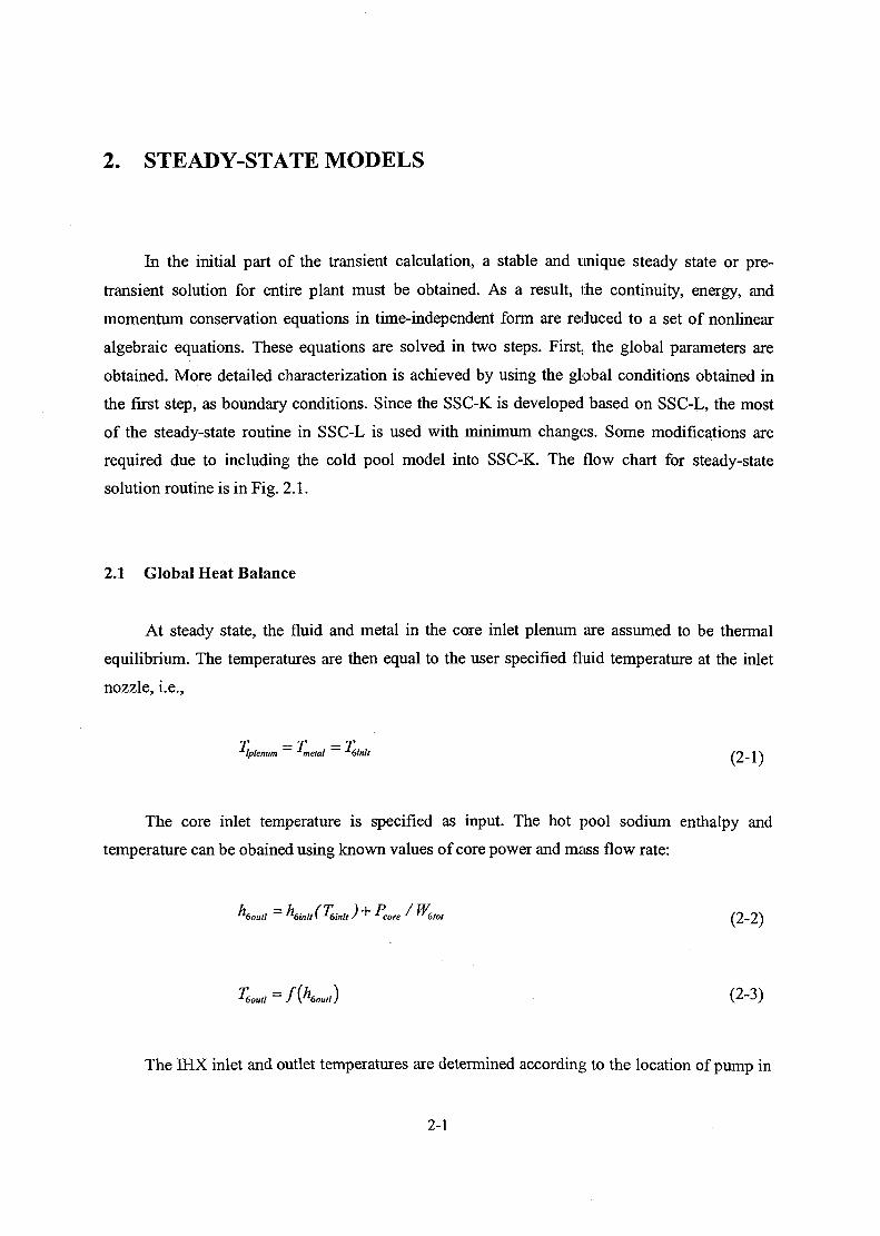
2. STEADY-STATE MODELS
In the initial part of the transient calculation, a stable and unique steady state or pre-
transient solution for entire plant must be obtained. As a result, the continuity, energy, and
momentum conservation equations in time-independent form are reduced to a set of nonlinear
algebraic equations. These equations are solved in two steps. First., the global parameters are
obtained. More detailed characterization is achieved by using the global conditions obtained in
the first step, as boundary conditions. Since the SSC-K is developed based on SSC-L, the most
of the steady-state routine in SSC-L is used with minimum changes. Some modifications are
required due to including the cold pool model into SSC-K. The flow chart for steady-state
solution routine is in Fig. 2.1.
2.1 Global Heat Balance
At steady state, the fluid and metal in the core inlet plenum are assumed to be thermal
equilibrium. The temperatures are then equal to the user specified fluid temperature at the inlet
nozzle, i.e.,
n"1 T"» y
Iplenum metal 6inlt (2-1)
The core inlet temperature is specified as input. The hot pool sodium enthalpy and
temperature can be obained using known values of core power and maiss flow rate:
Koutl = Kinlt (^linll) + Pcore ' ^6lot (2-2)
T6outl=f{h6mll) (2-3)
The IHX inlet and outlet temperatures are determined according to the location of pump in
2-1
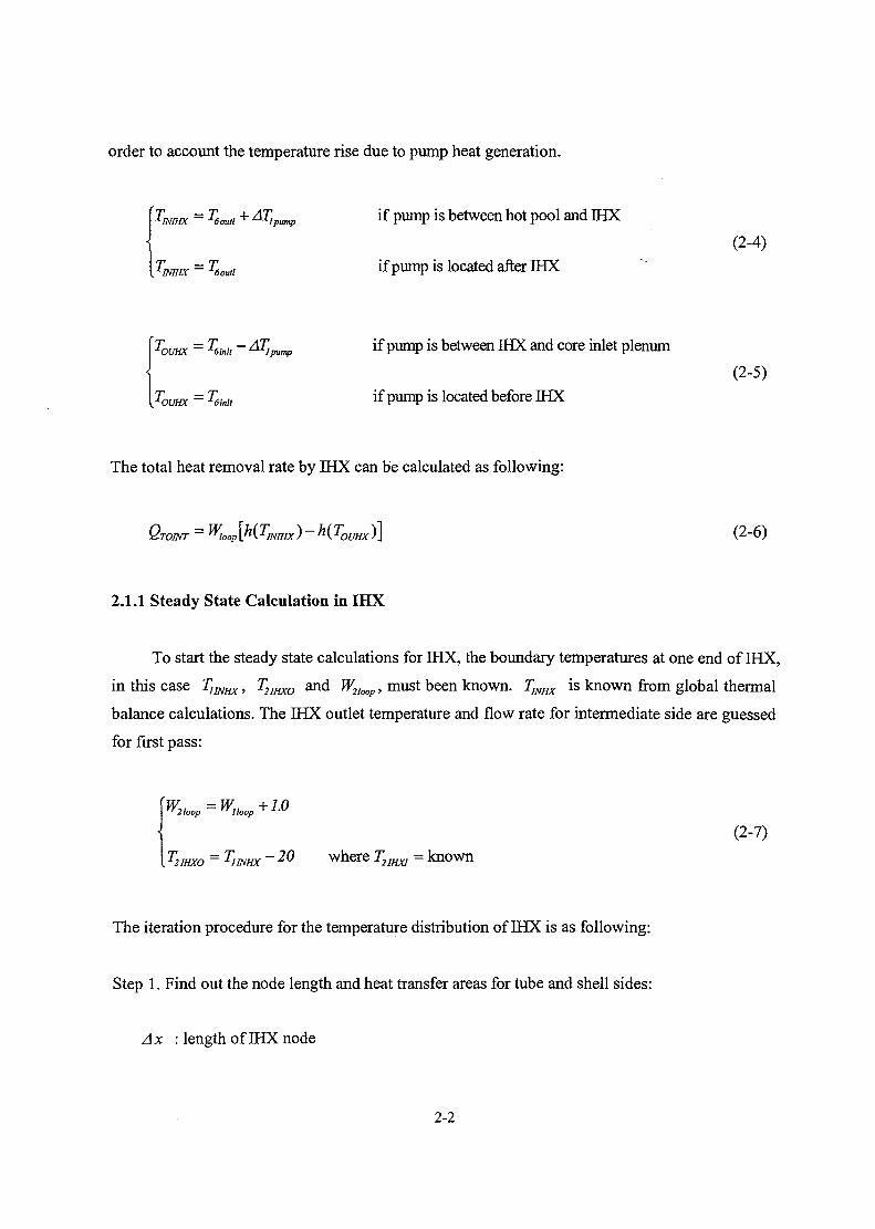
order to account the temperature rise due to pump heat generation.
\TINIHX = T6auii + ATIpimp ^ PumP is between hot pool and fflX
(2-4)= T6out, if pump is located after IHX
\Tomx = T6inIt - ATlpump if pump is between IHX and core inlet plenum
(2-5)~ T6MI if pump is located before IHX
The total heat removal rate by IHX can be calculated as following:
QTOINT = KoP[h(TiNmx)-h(TOUHX)] (2-6)
2.1.1 Steady State Calculation in IHX
To start the steady state calculations for IHX, the boundary temperatures at one end of IHX,
in this case T1JNHX, T2IHXO and W2loop, must been known. Timx is known from global thermal
balance calculations. The IHX outlet temperature and flow rate for intermediate side are guessed
for first pass:
\W -W +101 vr2hop rrIloop ^ 1 U
I T2IHXO = T,INHX ~ 2 0
The iteration procedure for the temperature distribution of IHX is as following:
Step 1. Find out the node length and heat transfer areas for tube and shell sides:
Ax : length of IHX node
2-2
(2-7)

A2 : primary side (shell side) heat transfer area for each IHX node
= n • (IHX tube outer diameter) -Ax-(# tubes)
A, : intermediate side (tube side) heat transfer area for each IHX node
Step 2. Compute the constants for computation of Peclet numbers:
APEP = (diameter) (velocity) (density) = Pe • k / cp = "oop—- (2-8)
W -dAPES = (diameter )(velodty)( density) = Pe-k/cp = -^—~ (2-9)
Step 3. Guess the tube structure temperature (Fig. 2.2):
T,.
2
(2-10)
P> Iso — Asi
Step 4: Calculate the node average sodium temperatures:
7f _TS0 + Tsi
» z2 , Z (2-11)
Step 5: Find out the non-dimensional numbers for heat transfer coefficients:
Peclet numbers for primary and intermediate sides
Pes=APES-cPs/ks (
Nusselt number
Nu =a + b-Pec Shell side (primary) (2-13)
2-3

Aoki's correlation for tube side (intermediate)
Nu, = 6.0 + 0.025 • CFPJ"-8 (2-14)
where
nnun-e j (2_i5)
M Ms
Step 6: Calcualte the overall heat transfer coefficients:
•P | r + r
Jr wall'P fo»'.P
Ust = —R (2-20)
Nus-ks wa"'s f0l"'s
Step 7: Calculate the node outlet temperatures for primary and intermediate sides:
w''lloop
A.-UJTT-TJ-*—£ (2-22)
2-4

TPo, = (2-23)
(2-24)
Step 8: Calculate the node average sodium temperatures and tube temperature based on the
calculated node exit temperatures:
T=Lpol T xpi (2-25)
— Trp _ •LSOl
2(2-26)
A2Upt(2-27)
Step 9: Perform the convergence test for the node:
if T —Tpo pol
and \TSO-Tsol\>s and TT -TT, >s then (2-28)
2 (2-29)
go to Step 4 and iterate again.
Step 10: Reset the node exit temperatures into the inlet temperatures for next node until
/ = nihxl:
Tpol->Tpi, Tsol^Tsi, TT,-+TT and go to Step 4 and continue for next node.
2-5

Step 11. Perform the error checking if the energy gain is equal to energy loss:
Ll0UHX ~ -* < e po / (2-30)
•'•2INHX
oss ~ "lloopiep,in ~
(2-31)
(2-32)
(2-33)
if 1--Qlloss
> s error (2-34)
Step 12. Check for convergence based on total energy balance:
The heat rejection from IHX should equal to the reactor heat plus heat addition at the
pump within specified limits:
if Q-TOINT Q-2%ain
Q:TOINT
< s quit interation (2-35)
Step 13. If not, the secondary outlet temperature and flow rate have to be reselected and the
computation repeated until convergence is obtained:
Log-mean temperature difference
AT —
~ *2OUHx)\(2-36)
= Q2gain/AT (2-37)
2-6

Assuming UA constant, determine new Imtd guess
^L (2-38)
'" (2-39)
ATnew = —p-^ ^ r •> Find ATB using root finding scheme. (2-40)ln[ATA/ATB\
Ql0INT
T2OuHx=TimHX-ATB (2-41)
- | Return to Step 1 (2-42)
After calculating the temperature distribution of IHX, the similar process is performed for the
energy balance for steam generator.
2.2 Hot Pool Pressure Distribution
Subroutine PINT IS calculates the interface pressure between the hot pool and IHX.
"lINLT
where Z6UPLN : relative height of sodium in vessel upper plenum to Z6REF
Z6ONOZ : elevation of vessel outlet nozzle above Z6REF
-*1INLT ~ *6OUTL (2-44)
"6OUTL = *1
*6INTL ~ *6OUTL "^ "lPDRV (2-46)
where PIPDRV '• pressure drop between core inlet and IHX inlet
2-7

2.3 Thermal-Hydraulics for Fuel Assembly Region
2.3.1 Core Thermal-Hydraulics
The core region is divided into N6CHAN parallel channels. These channels represent either
fuel, blanket, or control rods. The flow rate for each channel is obtained by user specified flow
fraction of the total flow through these channels.
(2-48)L6R0D.
where ^*6h '• mass flux of channel 7
N 6RODSJ : number of rods in channel y
A6RODJ : sodium flow area per rod in channel^
Each of the flow channels is divided into a user-controlled number of axial slices. The axial
distributions of coolant enthalpy and pressure in all channels are determined in this subroutine.
7 -W^6CHAN ''6CHAN,
where ^6TPOWS : Total normalized power fraction in channel j from fission and decay
heating
dhFACT)> d W6CHANj Z6CfIAN- (2-50)
— F • F - 7~ 1 CONSl 1 6NPWAjj ^
2-8

where QFACTJ, : enthalpy change in axial slice i of channel j
^JJ : normalized axial power in axial slice / of channely
J, : length of axial slice i in channel y
T +T1AVG
TOUT = + QFAcrlt ' Cp(TAVG) (2-52)
where Tin : inlet temperature of axial slice / in channely" (known)
TOLD : outlet temperature of axial slice i in channel^ (unknown)
T0UT : calculated outlet temperature of axial slice; / in channel^
if the temperature difference between initial guessing value and calculated value, \T0UT - TOLD\,
is greater than user specified limit, TOLD is reseted to TQUT and Tom is calculated again unitl
\TOUT - TOLD\ is less than the limit. Then, the friction and heat transfer coefficients are calculated
based upon the new outlet temperature of the axial slice.
,, = f[Dh,G6fj,ju(T0UT),(P/ D)wd,(P/ D)wirewrap,L6ATYP] (2-53)
Nu[Dh,G6Ij,TAVG,(PID)rod\K{TAVG)~ n (2-54)
After completing the calculations for the current axial slice, the same calculations performs for
the next axial slice.
2.3.2 Core Pressure Distribution
Because the current version of SSC-K simulates single phase flow, the flow is assumed to
be incompressiable. The axial distributions of coolant pressure in all channels are determined by
momentum equations.
2-9
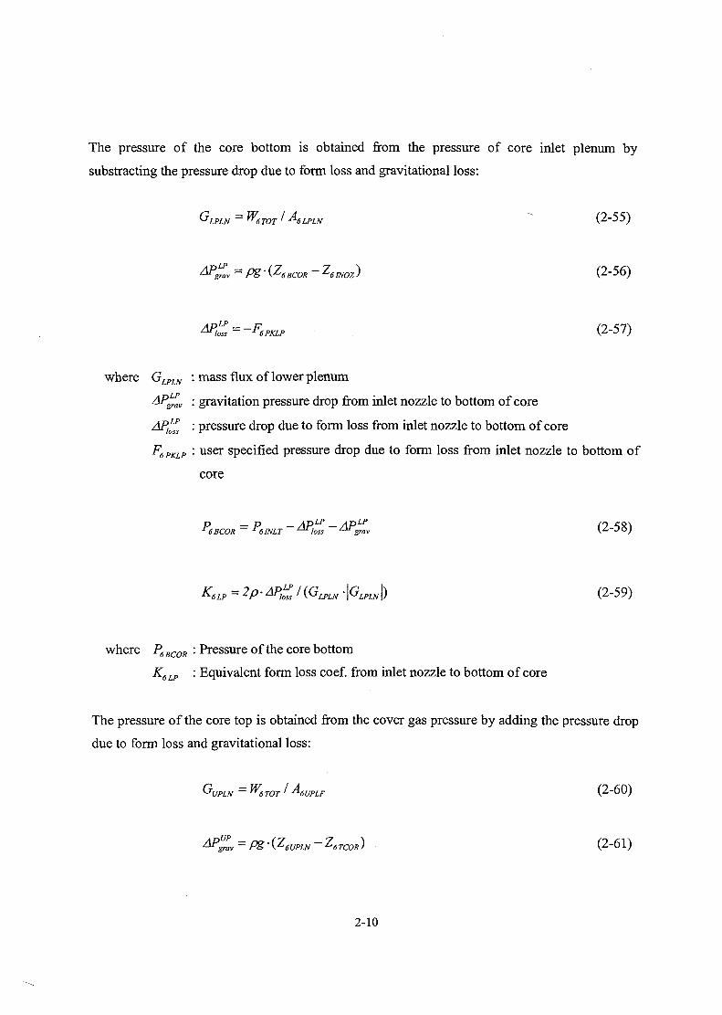
The pressure of the core bottom is obtained from the pressure of core inlet plenum by
substracting the pressure drop due to form loss and gravitational loss:
GLPLN ~ "6TOT ' -"6LPLN (2"55)
AP^v = PS • (Z6BCOR ~ Z6IN0Z ) (2"56)
(2-57)
where GLPLN : mass flux of lower plenum
gmv '• gravitation pressure drop from inlet nozzle to bottom of core
: pressure drop due to form loss from inlet nozzle to bottom of core
F6PKLP : user specified pressure drop due to form loss from inlet nozzle to bottom of
core
P6BCOR = P6INLT - *P£ ~ *P£ (2-58)
K6LP=2p-AP£l{GLPLN -\GLPLN\) (2-59)
where P6BCOR '• Pressure of the core bottom
K6LP : Equivalent form loss coef. from inlet nozzle to bottom of core
The pressure of the core top is obtained from the cover gas pressure by adding the pressure drop
due to form loss and gravitational loss:
' A6UPLF (2-60)
) (2-61)
2-10

(2-62)
where GUPLN : mass flux of upper plenum
APgmv '• gravitation pressure drop from top of core to top of hot pool
AP^S : pressure drop due to form loss from top of core to top of hot pool
F6PKUP : user specified pressure drop due to form loss from top of core to top of hot
pool
(2-63)
K6UP = 2p-APZl(GUPLN -\GUPLN\) (2-64)
where P6TCOR : Pressure of the core bottom
K6UP : equivalent form loss coef. from inlet nozzle to bottom of core
Before calculating the pressure distribution for the active core region, the pressre drop in inlet
orifice zone has to be estimated:
(2-65)
W • Fr'6TOT r6FLOWj
"INOZ, ~ •"SASSYj
where £P™£,z: Pressure drop for inlet orifice zone
^ZJ : flow rate per subassembly for channel^
wj: flow fraction for channel^
Because the pressure drop due to friction in inlet orifice zone is given by user, the hydraulic
diameter for orifice zone can be found by Bisection or Newton's method (YHYD6S).
2-11

1. Guess the initial value forZX1
2. Calculate the pressure drop due to friction
G\G\
A 2p(2-66)
3. Find the difference between user specified pressure drop and calculated pressure drop
APn+1=AP™coz-AP™'c
c (2-67)
4. Reset the upper and lower limits for Bisection method.
\ = AP"+!
\APLOW = APn+I
if AP"+I > 0.0
if APn+1 < 0.0(2-68)
5. Convergence test
if AP"+1 <1.0 then D™oz = Dh and terminate the iteration (2-69)
6. Find the hydraulic diameter for next iteration:
Dnh+I =Dn
h+AP"AP" -AP"
(2-70)
7. Test if Dnh
+1 is within the bounds.
Reset the values and return to step2
DT1 =2
Reset the values and return to step2
if
else
<Dnh+1 <Du
hp
(2-71)
2-12

Because the form loss coefficient due to expansion and contraction in inlet orifice zone is given
by user, the pressure drop in orifice zone can be obtained such as:
Mass flux for inlet orifice zone is obtained from the calculated hydraulic diameter:
Q _ 4'WINOZ
The pressure drop drop to form loss:
JNOZ
fi* _ f MJ
j,Ai -J6FRIC n
(2-73)2p
The pressure at the bottom of active core region is:
p — P _ APINOZ — APMOZ — AP'NOZ
r6 NODEj, ~ r6BCOR Zlrgrav ^^loss Zlrfric
The constant for calculation of the pressure distribution in active core region:
(2-75)
where pjt/jl : average density for nodes i and i+1 in chamnely"
(2-76)
2-13

c2 c2
U6I _ ^61 (2-78)Pj,M Pj,i
The pressure at node i+1 is:
P - P - Apsrav - APfric - Apr6 NODEj M — r6 NODEs)
Zlrj,Ai ^^j.Ai /iirj,Ai
2.3.3. Upper Plenum Thermal-Hydraulics
The core region is divided into N6CHAN parallel channels. These channels represent either
fuel, blanket, or control rods. The flow rate for each channel is obtained by user specified flow
fraction of the total flow through these channels.
N6CKiN
Z (2-80)
N6CHAN
\W6CHANj-E6NODE) W6CT (2-81)
[ N6CHAN \ /
2-j 6NODEj \/^6CHAN (2-82)
N6CHAN
(2-83)
The temperatures for cover gas, internal structure, thermal liner and vessel closure head can be
found by solving the governing energy equations for hot pool region by iterative procedure:
1. Guess thermal liner temperature, T6M2 same as hot pool sodium temperature:
2-14

T — f • T —f . f ——/16M2 ~ ±6OUTL> XUP •l6OUTL> ALOW Im
(2-84)
^ = & *6BPUI
2. Compute the temperatures for cover gas, internal structure, thermal liner from user-specified
heat transfer coefficients and the assmued thermal liner temperatun;:
\^6OUTL ~ •*6M2)/UAGM2 (2"85)ALM2\^6OUTL
*6CGAS + UAGM3*6BPU1)I^ " U AGM3 (2-86)
'ALMl^^AGMl) (2-87)
3. Compute T6M2
H (T —T } + II (T —T } + TJ (T —T \rp* _ JI uALGL\X6OUTL X6CGAS / T u AGM1\16M1 16CGAS / T u /<GMJV-ftfA/3 16CGAS) ,~ o o \
^^GM2
4. If computed T*6U2 is not equal to assumed T6M2, reset and iterate.
In order to calculate the pressure drop for outlet module, the core outlet pressure has to be found.
= P + p(T )g-(Z +Z ) (2-89)
*6TCOR ~ °6OUTL + P\^6OUTL)S'\^6ONOZ +^6TCOR/ (2-90)
where PSOUTL '• HX inlet pressure
PSTC0R : core outlet pressure
2-15

2.3.4 Core Outlet Module Hydraulics
This subrutine calculates the pressure equalization loss coefficient at outlet module.
iNOZj ~ ''6TOT 1 6 FLOWs j ^ 5 ASSY j (2-91)
' •*"5AR0Dm) (2-92)
where flow rate per assembly in channel/
mass flux per assembly in channel^
(2-93)
G OUZj Jouz,
P(2-94)
where ^^Moss,: pressure drop for outlet module zone in channel j due to contraction and
expansion
^AJ : k-loss factor for outlet module zone in channel j due to contraction and
expansion
AP - P -P - APom - AP0UT
/Lurs ~ r6N0DElasmxk 16TCOR i L " gravj ^klossj
(2-95)
KOUTj = F6LSA4j =2-AP£-p/(G0UZj •0UZj
(2-96)
where ^6isA4j: k-loss factor for outlet module in channel/ except k-loss due to expansion
and contraction
2-16

2.4 Loop Hydraulics
2.4.1 Hydraulics for IHX
This subroutine solves the steady state pressure drop and/or k-loss factor for the IHX.
The pressure drop due to flow differnece:
. PIHX,O PIHXJ
1HX
The pressure drop due to contraction or expansion at IHX inlet:
w \wmx' IHX
The pressure drop due to contraction or expansion at IHX outlet:
( 2 . 9 7 )
W-De— (2-98)
f = f(Re) (2-99)
The pressure drop due to wall friction:
The pressure drop due to gravitation:
= g\ PlHX.1 ' sin<t> IHX.l^lN + P IHX ,0 'S™<t>'iHX.O^OUT + ZiPi Sin fcAX; (2-101)
P - tr mxIHX /-oossin ~ Km — T T (2-
ZPin ' Ain
2-17

loss.out - Kout ~ -JT (2-103)
The total pressure drop except the pressure drop due to k-loss factor inside IHX:
*PSVM =APfloW + APfric+APgraV+M>loSsM+APloss,out (2-104)
The total k-loss factor for IHX except k-loss due to contraction and expansion:
KIHX=2pIHX(P1PDWC-APSUMs) A>™ (2-105)
"IHXY'IHX]
2.4.2 Hydraulics for Pipes
This subroutine solves the steady state flow equations for a pipe in the coolant loop. It is
assumed that the diameter is constant, and the pipe wall is in thermal equilibrium with the
coolant.
Axnode=Axpipe/NINODE (2-106)
NI NODE'1
SlnSUM = £ sink (2-107)
EOD = (Roughness) I De (2-108)
f = f(Re,E0D) (2-109)
The total pressure drop in a pipe can be expressed in two different forms depend on
locations. The pipe between IHX exit and pump inlet is not a real pipe and is used to minimize
the modification of the SSC-L. Therefore, the pressure drop for the pipe between IHX exit and
2-18

pump inlet includes the pressure drop due to gravitaion only. The density used in gravitational
force calculation is assumed as the cold pool sodium density.
l'oPE = Pddp • S-sinSUM-Axnode if pipe is between IHX exit and pump inlet (2-110)
+ Pinletg.sinSUMAxnode else (2-111)^PinletA
2.4.3 Pump
The pump rotating speed is determined by matching pump head and total hydraulic head.
The required pressure rise across pump is obtained from:
Ml PIPE
(2-112)
where AP^ : pressure drop for pipe i
P1PDRV : pressure drop from core inlet to IHX inlet
PIPDCV : pressure drop in check valve
The pump head:
l ) (2-113)
(2-114)
(2-H5)
(2-116)
2-19
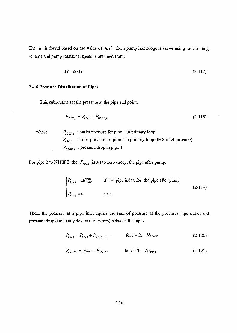
The a is found based on the value of hjv1 from pump homologous curve using root finding
scheme and pump rotational speed is obtained from:
O = aOr (2-117)
2.4.4 Pressure Distribution of Pipes
This subroutine set the pressure at the pipe end point.
"lOUT.J ~ "]/N,l ~ "DROP,! (2-118)
where PWUT I '• outlet pressure for pipe 1 in primary loop
P1M, : inlet pressure for pipe 1 in primary loop (IHX inlet pressure)
PDROP i '• P r e s s u r e ^ P m
For pipe 2 to N1PIPE, the P1INJ is set to zero except the pipe after pump.
P!INJ = AP™°p ifi = pipe index for the pipe after pump
(2-119)p,iN,i = 0 else
Then, the pressure at a pipe inlet equals the sum of pressure at the previous pipe outlet and
pressure drop due to any device (i.e., pump) between the pipes.
, for/= 2, NIPJPE (2-120)
-PDROP, for/= 2, N1PIPE (2-121)
2-20

2.4.5 Cold Pool Hydraulics
The sodium enthalpy in cold pool is assumed to the IHX exit enthalpy.
Kp=hXcu, (2-121)
The liquid level in cold pool is obtained from pressure difference between the cover gas pressure
and the pump inlet pressure.
P — P
Ppin'S(2-122)
Then, the cold pool sodium mass is obtained from the sodium level in cold pool by assuming that
the cold pool can represented by two distinct regions with different cross-sectional area:
*bb-pmp
b-pmp
' cldp-c
p-c ' ( ^cp ~
if 2cp>ZXo
X Zcp<ZXo
(2-123)
2-21

MAIN9S
PINT1S
C00L6S
FUEL5S
L00P1S
PRNT9S
IHX1S
STGN3S
0PTN6S CORE6S
PRES6S
UPLN6S
FLSA6S
w
w
'WDFfi-S^
PIPEtS'
END1S
PUMP1S
PRES1S
RES1S.--
RITE1S
if IHX
if normal pipe
fori =1, # channel
for i =1, # pipes
modified unchanged
Fig. 2.1 Flowchart for Steady-State Calculation
2-22

Primary Flow
Shell wall (assumed insulated)
Tpi+
Tube wall
Secondary Flow T — w.
Known Unknown
Fig. 2.2 Steady state Conditions for an IHX Nodal Section
2-23
3. TRANSIENT MODELS
The dynamic response of the primary coolant in a pool-type LMR, particularly the hot pool
concept like KALIMER, can be quite different from response in the loop-type LMR. The
difference arises primarily from the lack of direct piping connections between components in the
hot and cold pools. Even through there are free surfaces in the reactor vessel and pump tank of
loop-type designs, the direct piping connections permit the use of basically a single momentum
equation to characterize the coolant dynamics in the primary loop, except in a transient initiated
by pipe rupture or similar asymmetric initiator.
In KALIMER, both hot and cold pools have free surfaces and there is direct mixing of the
coolant with these open pools prior to entering the next component. At least two different flows
would have to be modeled to characterize the coolant dynamics of the primary system. During
steady-state the two flow rates can be obtained by a simple algebraic equation. During a transient,
however, the flow from the pump to hot pool would respond to the pump head and losses in that
circuit including losses in the core; the IHX flow would respond to the level difference between
the two pools, as well as losses and gravity gains in the IHX. The gravity gain could be
significant for low-flow conditions, particularly if the IHX gets overcooled due to a mismatch of
primary and secondary flows. The flow chart for transient routine is in Fig. 3.1.
3.1 Flow Equations
Since the primary system of KALIMER has same number of pumps and IHXs, the first
version of SSK-K has developed with constraint that the number of pumps has to be same as the
number of IHXs. In SSC-K, the concept of flow paths (Npath) is introduced and each flow path
includes one pump and one IHX.
3.1.1 Intact System
For an intact system, volume-averaged momentum equations can be written as follows:
3-1

Pump Flow
(3-D
In above equation, the pump exit pressure, PPo, is obtained from
P = P +0 2 H (3-2)Po Pin r Pin& xx VJ z ' /
where H is the pump head, obtained from the pump characteristics.
IHXFlow
dW,Ak) v-> L(k) n xr^ . „ , , . ,
dt ^
The IHX inlet and exit pressures, PXm and PXo, are obtained from static balance as
~ZXin) (3-4)
~ZXo) (3-5)
The core inlet pressure, PRin, is obtained from a complicated algebraic equation and the
derivation will be discussed later.
3.1.2 Damaged System
In KALIMER, the pipe rupture can only happen in pump discharge line to reactor core. For
the broken path, Eq. (3-1) has to be modified to:
3-2

uob • / 1 uob
An additional equation is needed to describe the flow downsteam of the break:
(3-7)dob A dob
The inlet and outlet pressures at break location, Pb!n and Pbo, respectively, are calculated
by break model. The break model in SSC-K is same as that in SSC-L. The external pressure for
the break, which is needed to compute these pressures, is obtained from static balance as
(3-8)
This pressure acts as the back pressure opposing the flow out of the break. The value of
this pressure is much larger than that for loop-type design, which is generally equal to
atmospheric pressure until the sodium in guard vessel covers the break location. This will
make the pipe break in pool-type designs less sever relative to loop-type designs.
3.2 Pump Suction Pressure
Fig. 3.1 shows a schematic of SSC-K Modeling for KALEMER. As you may be noticed,
there is a pipe after IHX which does not exist in KALIMER. This pipe is included to minimize
the modification of loop type version of SSC-K. This pipe is used to make the elevation of IHX
exit same as the elevation of pump inlet. The pump surge tank model in loop-type version of
SSC is used as a basis of the cold pool model in KALIMER. Pump surge tank in a loop-type
LMR has similar characteristics with cold pool in pool-type LMR in many aspects. Both
components include two distinct regions. In one region, the sodium is present in lower part while
the second region is filled with noncondensable gas on the top of the sodium. The sodium levels
in both components are changing with mass balance between IHX exit flow and pump inlet flow.
However, some differences exist between two components. First, cover gas in pump surge tank is
separated by cover gas in vessel while cover gas in cold pool is in common with cover gas above
hot pool. Second, enthalpy in pump surge tank is assumed to be same as enthalpy of IHX exit
3-3

flow. This is a reasonable assumption for pump surge tank because of its small volume. However,
it is not true in cold pool, which has relatively large sodium inventory. Therefore, energy
equation is added in cold pool model to account the energy stored in sodium. And it is assumed
that the entire pump inlet flow is from cold pool and no direct flow from IHX exit. The energy
balance in cold pool will be discussed in later section.
As seen in Fig. 3.2, a few variables are newly defined to model a cold pool and their descriptions
are as follows:
- V6BPMP: Volume below pump inlet
- Z6IHXP: Elevation change from pump suction to IHX exit
- A6IHXP: Average flow area from pump suction to IHX exit
- A6OVRF: Average flow area for overflow path
- B6CLDP: Sodium mass of cold pool
- E6CLDP: Sodium average enthalpy of cold pool
- T6CLDP: Sodium average temperature of cold pool
- D6CLDP: Sodium average density of cold pool
The pump inlet pressure is obtained by adding cover gas pressure with elevation head of cold
pool:
Pp,n = Pps+PcgiZcF-Zpu.) (3-9)
3.3 Liquid Levels in Pools
The liquid levels in cold and hot pools can be obtained by mass balance at each pool. The
total flow through all the IHXs and all the pumps can be determined from:
(3-10)k=\
and
3-4

•or _ \ vy (''Ptot ~ / ,"p\
k=\
(3-11)
Total sodium mass in cold pool is obtained by mass balance at the cold pool:
= Wxtot -WPtot+Wovf + Wb (3-12)
Note that the break flow, Wb, is zero for an intact system and the overflow from hot pool, Wovf,
is zero if the hot pool level is below the top of thermal liner. Then, the cold pool level can be
obtained from the sodium mass in cold pool by assuming that the cold pool can represented by
two distinct regions with different cross-sectional area:
(pV)a> =
Pepybp jHXP• \Zcp Z
IHXP
i f ( p V ) C P > p c p • (Vbpmp + A m x p • Z m x p )
(3-13)
if
where Vbbpmp
A m x p
JHXP
Aovf
: Cold pool volume below flow skirt
: Average cold pool cross-sectional area between flow skirt botton
and IHX exit
'• Height from flow skirt botton to IHX exit
: Average cold pool cross-sectional area above IHX exit
The time rate change of sodium mass in hot pool is obtained by mass balance at the hot pool:
= Wc -Wxto, - Wovf (3-14)
Eq. (3-14) assumes that all the level changes likely to occur during the transient are confined to a
constant cross-sectional area. When equations (3-12), (3-13) and (3-14) are solved
3-5

simultaneously with the flow equations, the sodium levels for hot and cold pool during the
transient can be obtained.
3.4 Reactor Internal Pressure
The reactor internal pressure, PRln, for both an intact and a damaged system is derived in
the following section.
3.4.1 Intact System
Mass conservation at core inlet yields
k=\
Differentiating both sides with time yields
The core flow can be expressed in terms of channel flows as
W3 (3-17)7=1
where Nch represents the number of channels simulated in the core. Differentiating both sides
with time gives
Time rate of core flow change for each channel can be written from momentum balance
3-6

dt(3-19)
(3-20)
Combining Eqs. (3-16), (3-18) and (3-19) gives
k dt • <-,(3-21)
Substituting Eq. (3-1) into the left hand side of Eq. (3-21) gives
Ek=\
PPo(k)-PRin-
L(k),A(k)
Y(3-22)
Simplifying Eq. (3-22) yields the core inlet pressure as
P =Rin C+D
(3-23)
where
,, (3-24)
"poll,
E (3-25)
3-7

(3-26)
(3-27)
3.4.2 Damaged System
In case of a pipe rupture in one of the pump discharge lines, mass conservation at core inlet
has to account for the downstream flow of break to core.
(3-28)k=l*brk
Differentiating both sides with time yields
dWc _dt
dWp(k) dWdob
dt dt(3-29)
Combining Eqs. (3-19 and (3-29) gives
dt(3-30)
Substituting Eqs. (3-1) and (3-7) into the left hand side of Eq. (3-30) gives
3-8

£*brk
PpoW- PRU
vlaP
P
L(k)A(k)
Pf-sWdob
=z-(3-31)
Simplifying Eq. (3-31) yields the core inlet pressure as
A+B+CD+E+F
(3-32)
where
(3-33)
k=\*brk
(3-34)
c=- rfoi
rfot
(3-35)
(3-36)
(3-37)
3-9

dob
3.5 Energy Balance in Hot Pool
Thermal stratification can occur in the hot pool region if the entering coolant is colder than
the existing hot pool coolant and the flow momentum is not large enough to overcome the
negative buoyancy force. Since the fluid of hot pool enters IHXs, the temperature distribution of
hot pool can alter the overall system response. Hence, it is necessary to predict the pool coolant
temperature distribution with sufficient accuracy to determine the inlet temperature conditions
for the IHXs and its contribution to the net buoyancy head.
During a normal reactor scram, the heat generation is reduced almost instantaneously while
the coolant flow rate follows the pump coastdown. This mismatch between power and flow
results in a situation where the core flow entering the hot pool is at a lower temperature than the
temperature of the bulk pool sodium. This temperature difference leads to stratification when the
decaying coolant momentum is insufficient.
The stratification of the core flow in the hot pool is represented by a two-zone model based
on the model for mixing in the upper plenum of loop-type LMRs in SSC-L (Fig. 3.3). The hot
pool is divided into two perfectly mixing zones determined by the maximum penetration distance
of the core flow. This penetration distance is a function of the Froude number of the average core
exit flow. The temperature of each zone is computed from energy balance considerations. The
temperature of the upper portion, TA, will be relatively unchanged; in the lower region, however,
TB will be changed and somewhat between the core exit temperature and the temperature of
upper zone due to active mixing with core exit flow as well as heat transfer with the upper zone.
The temperature of upper zone is mainly affected by interfacial heat transfer. Full penetration is
assumed for flow with positive buoyancy.
The two-zone model in SSC-L has some difficulties to maintain the mass and energy
conservation in the hot pool because it does not account for the mass and energy change due to
3-10

the variation of penetration height. Therefore, the following equations for energy balance is
adopted in SSC-K.
The non-conservative form of energy balance equations which determine the various
temperatures in the hot pool are given below:
3.5.1 Lower Mixing Zone B:
dz,Casel: -^-
dt
Mass conservation
,WIHX{k) (3-39)
Energy Conservation
d dz. ^L— (pEV)B = -^-pAAEA + WrERn ~fB y WmxEB
-UAbm2{TB -Tm2)-UAhna(l-f)(TB -Tj-hA^T, -TA)
Expand derivative in energy equation for total mass and enthalpy:
dz Npath
^AEWE f y+ EB(pV)BpAAEA+WcERo fB ywrffYEBdt B dtKH )B dtHA A c Ro JBtt IHX B (3-41)
Combine above equation with mass conservation equation and rearrange the nonconservative
form of energy equation:
3-11
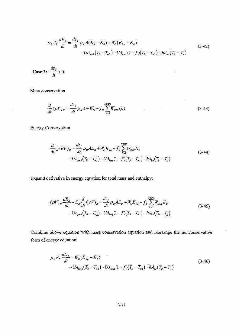
pAA(EAEB) + Wc(EsEa)dt dtFAKA B) cK Ro B) (3-42)
dZ;Case 2: -^-
dt
Mass conservation
d , _ dzJf{pV)BtpBA + WcfBYJWIHX{k) . (3-43)dt dt t{
Energy Conservation
j J - Npath
— {pEV)B = —LpBAEB + WcERo - / . Y WIHXEBdtH )B dtHB B c RO JB/_, mx B
Expand derivative in energy equation for total mass and enthalpy:
dF d dz Npath
^ E(V)=^pBAEB+WcERo-fB Y,WmxEB
Combine above equation with mass conservation equation and rearrange the nonconservative
form of energy equation:
-UAbm2{TB-Tm2)-UAhmX{\-f){TB-TmX)-hAba(TB-TA)
3-12

3.5.2 Upper Mixing Zone A:
C a s e l : — -dt
Mass conservation
dz, N^lh
{pV)Aj;PAfA Y^mx^)-WorS (3-47)dt dt k=1
Energy Conservation
j JU Npath
-iPEV)A =-i;P<AEA -fA X
-TA)
Expand derivative in energy equation for total mass and enthalpy:
dF d dz Npalh
^ + E{V)^AEfjyiHXEA-WorfEA
Combine above equation with mass conservation equation and rearrange the nonconservative
form of energy equation:
~f- = -UAam2(TA-Tm2)-UAhmlf(TA-Tml)
-UAhg(TA-Tg) + hAba{TB-TA)
dz-Case 2: — -
dt
3-13
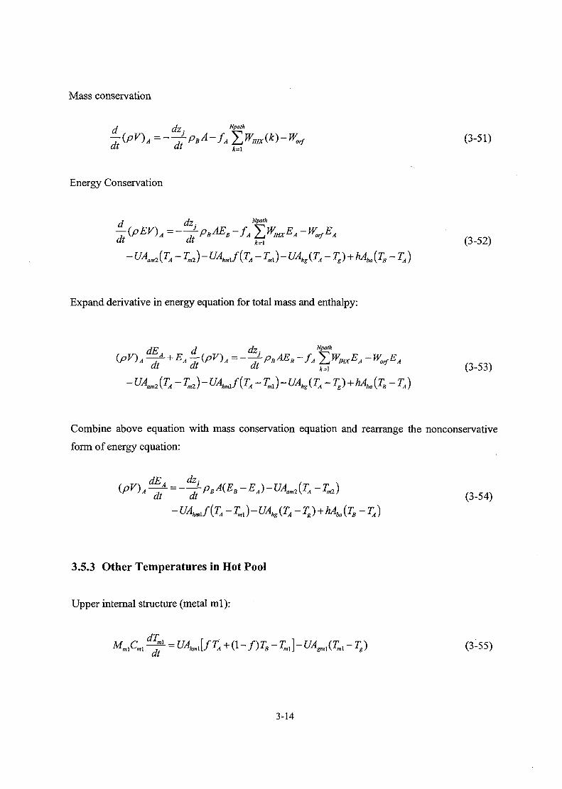
Mass conservation
dz:Worf (3-51)
Energy Conservation
d dz Npath
-{pEV)A =-~LpBAEs-fA YW,HXEA -WorfEA<M at
Expand derivative in energy equation for total mass and enthalpy:
dF d d.Z 'Npath-JT + EA -JSPV)A =--j-pBAEB - / , ^lWBaEA -WorfEA
ai ai at k^x
-UAaml{TA-Tml)-UAhmj{TA -T^-UA^
Combine above equation with mass conservation equation and rearrange the nonconservative
form of energy equation:
E^UA"^ O (3.54)-UAhmj{TA-TmX)-UAhg{TA-Tg)
3.5.3 Other Temperatures in Hot Pool
Upper internal structure (metal ml):
(3-55)
3-14

Barrier (metal m2):
ml _TJAhml\
Abm2TB
Ah ml
-UAcm2(Tm2-TCP) (3-56)
Uhm2 is not very sensitive to changes in sodium temperature, and so this equation is derived
assuming Ubm2 = Uam2.
Roof (metal m3):
Mm3Cm3 Tmi) (3-57)
The heat transfer from the roof to the ambient has been neglected.
Cover gas:
+ UAgml(Tml-Tg)-UAsa3(Tg-Tm3)
The auxiliary equations required by the above governing equations are
= \-Zj(t)l{ZHP-ZRo)
(3-59)
(3-60)
3.6 Energy Balance in Cold Pool
Currently, perfect mixing of the IHX flow with the cold pool sodium is assumed. Energy
balance equation for cold pool is derived as:
3-15
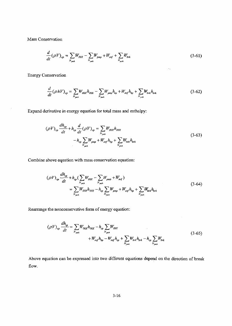
Mass Conservation
"pa*
Energy Conservation
d
-KN
path
Combine above equation with mass conservation equation:
"pa,h
Rearrange the nonconservative form of energy equation:
~ KP
dt {Ph V\p = ^ WIHXh[HX - ^ Wpmphcp + Wovfhhp + ^ Wbrkhbrk (3-62)" path path ™ path
Expand derivative in energy equation for total mass and enthalpy:
(3-63)
(3-64)Krk
(3-65)
Above equation can be expressed into two different equations depend on the direction of break
flow.
3-16

Npah
"path
ifWbrk>0 (3-66)
Discretize above equation in time:
At
(PV)CP~C >
- W h'+&1 + ^W h - ht+At V Wyrmfncp ^ Z_i V'brknbrk ncp Z-i brk
''pah
Aty'l 1HX"IHX "cp / _ f 1 H X
Npah
ifWbrk<0
(3-67)
At
At
At
"pa*
Z"pail,
ovf
(3-68)
3-17

Solve for tic+/ :
h' +
(3-69)
Lower structures (metal m4):
(3-70)
It should be noted that the heat transfer between structures and cold pool sodium is ignored in
current version of SSC-K. The above equation will be adopted in later version.
3-18
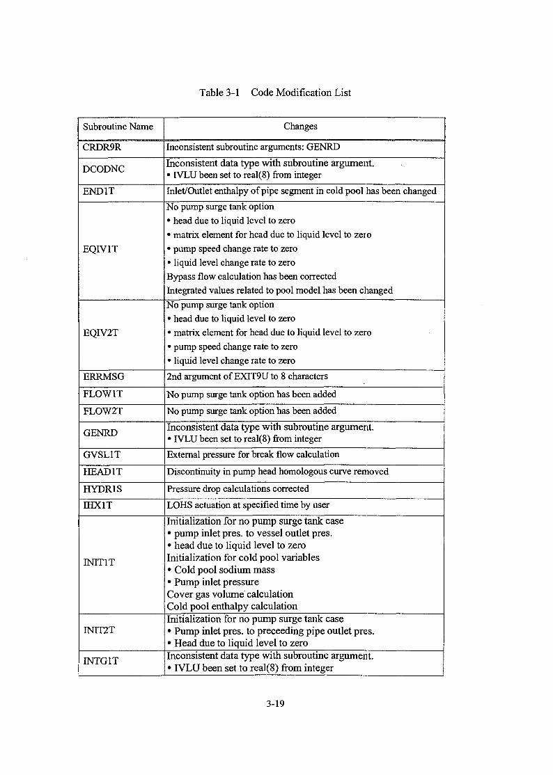
Table 3-1 Code Modification List
Subroutine Name
CRDR9R
DCODNC
END1T
EQIV1T
EQIV2T
ERRMSG
FLOW1T
FLOW2T
GENRD
GVSL1T
HEAD1T
HYDR1S
IHX1T
INIT1T
INIT2T
INTG1T
Changes
Inconsistent subroutine arguments: GENRD
Inconsistent data type with subroutine argument.• IVLU been set to real(8) from integer
Inlet/Outlet enthalpy of pipe segment in cold pool has been changed
No pump surge tank option• head due to liquid level to zero• matrix element for head due to liquid level to zero• pump speed change rate to zero• liquid level change rate to zeroBypass flow calculation has been correctedIntegrated values related to pool model has been changed
No pump surge tank option• head due to liquid level to zero• matrix element for head due to liquid level to zero• pump speed change rate to zero• liquid level change rate to zero
2nd argument of EXIT9U to 8 characters
No pump surge tank option has been added
No pump surge tank option has been added
Inconsistent data type with subroutine argument.• IVLU been set to real(8) from integer
External pressure for break flow calculation
Discontinuity in pump head homologous curve removed
Pressure drop calculations corrected
LOHS actuation at specified time by user
Initialization for no pump surge tank case• pump inlet pres. to vessel outlet pres.• head due to liquid level to zeroInitialization for cold pool variables• Cold pool sodium mass• Pump inlet pressureCover gas volume calculationCold pool enthalpy calculation
Initialization for no pump surge tank case• Pump inlet pres. to preceeding pipe outlet pres.• Head due to liquid level to zeroInconsistent data type with subroutine argument.• IVLU been set to real(8) from integer
3-19

Table 3-1 Code Modification List (continued)
Subroutine Name
ISETHM
LOOP1T
NSKIP
PBAL9S
PIPE1S
PEPW1T
PRUP6T
PUMP1S
PUMP IT
READ1R
READ7R
READ8R
READ9R
READ9T
READHM
REPEAT
Changes
Character variables can not be set to real variables directly.• Character variables are set to real variables using writestatement.Cold pool enthalpy calculation
Inconsistent data type with subroutine argument.• IVLU been set to real(8) from integer.ERR9U arguments been changed• sequence of arguments has been changedEnthalpy and pressure drop calculation routine for cold pool added
Pressure drop calculation routine for cold pool added
Calculation for IHX inlet pressure been corrected
Discontinuity of head homologous curve been corrected
Discontinuity of head homologous curve been correctedEMP coastdown at specified timeNo enthalpy rise across EMP assumed
GENRD arguments been changed : 19 places• 4th arg.: integer(id2) to real(d2)GENRD arguments been changed : 43 places• 4th arg.: integer(id2) to real(d2)GENRD arguments been changed : 1 place• 4th arg.: integer(id2) to real(d2)GENRD arguments been changed : 1 place• 3rd arg.: real(dum) to integer(idum)• 5th arg.: real(dum) to first real array element[a(l)]• 6th arg.: real(dum) to first int array element[ia(l)]int. array for data containment[ia(l)] been includedGENRD arguments been changed : 7 places• 4th arg.: integer(id2) to real(d2)equivalence statement (A(l)JA(l)) been removedGENRD arguments been changed : 1 place• 3rd arg.: real(dum) to integer(idum)• 5th arg.: real(dum) to first real array element[a(l)]• 6th arg.: real(dum) to first int array element[ia(l)]GENRD arguments been changed : 3 places• 4th arg.: integer(id2) to real(d2)error message for excess of max. table length been removedCharacter variables can not be set to real variables directly.• Character variables are set to real variables using writestatement.Inconsistent data type with subroutine argument.• IVLU been set to real(8) from integer.
3-20

Table 3-1 Code Modification List (continued)
Subroutine Name
RES1S
RESIT
RES2S
RES2T
RITE6U
UPLS6T
VERR9T
VESL1T
VRFY9T
WIMPLT
Changes
Steady state calculation for cold pool
No pump surge tank option has been added• liquid level in pump tank to zero• pump inlet presssure to vessel outlet pres.• liquid level change rate to zero
Cold pool option added• Time derivative of cold pool sodium mass• Cold pool level calculation• Pump inlet pressure
No pump surge tank option• gas mass in surge tank to zero• liquid level in surge tank to zeroNo pump surge tank option• liquid level in pump tank to zero• pump inlet pres. to vessel outlet pres.• liquid level change rate to zeroint. variables HY, HI been defineddefinition for character STRING 1 been changed• Overflow model added• Mass, energy equations changed to include overflow effect• Time derivative of enthalpy difference due to overflowmodified
Dimension for character NAME been changed to character*6
Overflow rate calculationCover gas volumecharacter NC been definedVERR9T arguments been changed : 11 places• 4th arg.: integer(+O) to character(NC)VERR9T arguments been changed : 1 place• 4th arg.: null character to character(NC)Cover gas volume calculation
3-21

MAIN9T INIT9T INIT6T
PRET1T |
INIT5T
INIT8T
COUR9T
DEFN1T
XI1T
INTG1T
DRIV9T |—•-• I D R I V i f ] — r - » | REAC5T
) FUEL5T
\ COOL6T~
{-tOOPtT~
LOOP2T
SAVE9f
PRNT9T
COEF6T
PIPE1T
END2T
PIPE2T
DEFN1T
PDFG1T |—r-»|- PIPW1T7]
HYDR1T
CVAL1T
PLOS1T
XJ—•{\
UPLN6T
FLOW6T
PRES1T
FIINCIT
BREK1T
PRUP6P
VJ1T
modified unchanged
Fig. 3.1 Flowchart for Transient Calculation
3-22

Hot Pool
Outlet Plenum
A
DRtVER
T
AHOT
DB1VER
T
Ai
8LANKET
T
AR
BALBKET
T
AcoNTROI
T
AREFUEcTOR
T
A
sH1EL0
TInlet Plenum
Cold Pool
Fig. 3.2 Schematic of SSC-K Modeling for KAUMER
3-23
Time: t Time:
Upper MixingZone: A
Lower MixingZone: B
trWr
'mx
'mxk=\
Upper MixingZone: A
dz
Lower MixingZone: B
trwc
Fig. 3.3 Two Mixing Zone Model for Hot Pool
3-24

4. INTERMEDIATE HEAT EXCHANGER
4.1 Pool Type IHX
The intermediate heat exchangers (IHX) physically separate the radioactive primary
coolant from the non-radioactive intermediate coolant while at the same time thermally
connecting the two circuits in order to transfer the core heat to the steam generator. The IHX in
pool type LMFBR is identical in function, and similar in design, to that in loop type design. The
only difference arises from the different configuration in the primary system, where the IHX
draws coolant from an open hot pool and discharges to another open cold pool. The liquid levels
in the hot and cold pools reflect the hydraulic flow resistance through the IHXs. The liquid level
difference in the KALIMER is about 5 m under normal operation. The low differential level
requires the IHX to have a low pressure drop on the primary side. The main concern with a low
pressure drop in the IHXs is its effect on flow distribution. Poor flow distribution can adversely
affect operational reliability by causing temperature distributions and resultant thermal stress that
could exceed design allowances.
Most of IHX in LMFBRs are of similar design. The IHX design of KALIMER is vertical,
counter flow, shell-and-tube heat exchangers with basically straight tubes as shown in Fig. 4.1.
Primary sodium flows downward on the shell side and exits at the bottom, with transferring heat
to secondary coolant in the tubes. The secondary coolant flows in the tubes. The pressure losses
in the primary side are limited as discussed above, it may be advantageous to send primary flow
through the tubes to ensure good flow distribution. The higher pressure in the secondary side is
to assure no radioactive coolant enters the secondary circuit in the event of a leak in any of the
heat transfer tubes.
Principal differences in IHXs between the loop and pool systems appear at the entrance
and exit flow nozzles. Tube bundle is mounted to allow for diffsrential thermal expansion
between the tubes and the shell. To accomplish this, the lower tube sheet is allowed to float and,
therefore, is supported by the tube bundle. The tubes are supported by the upper tube sheet.
4-1

4.2 Heat Transfer Model
The IHX model of SSC-K is essentially unchanged from that of SSC-L. The energy
equations are written using nodal heat balance with the donor-cell differencing scheme. Figure 3-
2 is a nodal diagram for thermal model under counterflow arrangement. The active heat transfer
tubes are modeled by one representative tube in the figure. The active heat transfer tube is
divided into same axial distance by user specified number. Axial heat conduction in the metal
wall is assumed negligible. As shown in Fig. 4.2, the IHX is modeled by four radial nodes,
secondary coolant, tube metal, primary coolant and shell wall. Material properties and heat
transfer coefficients are evaluated locally by specifying the material as user input. The tube and
shell wall nodes lie in the mid-plane between the fluid nodal interfaces, giving rise to a staggered
nodal arrangement.
The coolant equations are derived using the nodal heat balance method. It is assumed that
ideal mixing plenums at the inlet and outlet of each coolant stream. The time dependent
governing equations for thermal transportation of each section are described below.
1) Primary inlet plenum
PiJin~K) = Wp{epin-epx) (4-1)
where
* * = <TP ) a n d e*
Vin is the stagnant sodium volume in the primary inlet plenum, and p™ is the average sodium
density in the inlet plenum. Considering the fraction of flow bypassing the active heat transfer
region, (3P, we have the following equation from mass conservation.
W'p = (l-J3p)Wp
1) Primary outlet plenum
4-2

(4-4)Ul
Vout is the sodium volume in the primary outlet plenum and pout is the average sodium density in
the outlet plenum.
3) Primary bypass plenum
PPB ' pB ~T \ePB ) = P P "p \epm ~ e
PB ) (4-5)
Similar equations can be written for the inlet, outlet plenums and downcomer on the secondary
side.
4) Active heat transfer region
For primary coolant
For secondary side coolant
pV.~{es) = Ws(e, -e.) + UstAsl(T. -T ) (4-7)
For tube wall
, q jt{Tt) = UptApt{TPiM-Tt)-UstAst{Tti -TS/J (4-8)
For shell wall
MshCshi j t (Tshi) = UpshApsh(TPiM - Tshi) (4-9)
4-3

In the above equations, Vp and Vs are the control volumes between interfaces i and i+1 on the
primary and secondary sides, respectively. Apt, Ast and Apsh are the areas per length Ax for heat
transfer between primary coolant and tube wall, between secondary fluid and tube wall, and
between primary coolant and shell wall, respectively, defined as
Apt=xD2ntAx (4-10)
4 , = 7zrZV,A* (4-11)
(4-12)
where nt is number of active heat transfer tubes and ASh is the shell heat transfer area given by
user input. Di and D2 are the IHX tube inner and outer diameters, respectively, and L is the
length of the active heat transfer region.
In above equations, Upr, Ust, and UpSh represent the overall heat transfer coefficient between
primary coolant and tube wall, between secondary fluid and tube wall, and between primary
coolant and shell wall, respectively. Those are defined based on the thermal resistance concept
as:
(4-13)
(4-14)
(4-15)
where the film heat transfer coefficients are calculated in terms of Nusselt number Nu, which is
obtained from the embedded correlations in SSC-K. Fouling is a time-dependent phenomenon,
and the fouling resistances of l/hf0UijP and l/hf0Ui,s are provided as a user input quantity for the
primary and secondary sided walls, respectively.
1
1
1
upsh
1
Jibn,P
1
1hfilm ,P
1foul,p
1
"•foul,s
4-4

* A (4.17)D,
The wall thermal resistance terms are defined by dividing the tube wall thickness equally
between primary and secondary sides. The temperature of tube, Tt, is defined at the midpoint of
wall thickness.
(4-18)
(4-19)
where kt is a thermal conductivity of tube wall which is calculated internally by specifying the
material as input.
The overall heat transfer coefficients Upt and Ust are dependent on material and flow
properties, which are functions of temperature. Those are evaluated at each nodal section along
with the temperatures. Referring to Fig. 4.2, for each i, kt is evaluated at i on the tube wall node
whereas all other variables (kp, ks, Nupt, Nust) are evaluated at the midpoint between the fluid
nodal interfaces i and (i+1).
If a flow area on primary side of IHX is not provided as a user input, SSC-K calculates it
by the following equation. The pitch-to-diameter P/E>2 is taken to be as the average value in case
the pitch is not uniform throughout the tube bundle.
7rD
it
4-5

Then, the hydraulic diameter of primary side is calculated as follows:
'" " ' ^ (4-21)
The Reynolds number for the primary side and internal tube is defined as, respectively.
A"M" (4-22)
Re =A uAsMs (4.23)
where, the flow area through the tubes is given as
4 (4-24)
4.3 Pressure Losses Model
Figure 4-1 shows the flow paths of KALIMER IHX. Primary coolant flows downward in
the active heat transfer region and exits at the bottom of the tube unit. The secondary
(intermediate) coolant flows down the central downcomer into the bottom header (inlet plenum
region) where it turns upward to present a counterfiow arrangement in the heat transfer region. In
all cases, the primary flow is downward, and this helps to simplify the formulation. The sum of
pressure losses on both primary and secondary sides of the IHX is expressed as follows:
(APf;g)IHX = (acceleration loss) + (frictional loss) + (gravity loss or gain) + (inlet loss)+ (exit loss) + (contraction/expansion losses) +(other losses)
Note that a negative value obtained for gravity loss indicates a gain. The user should be
cautious when specifying the value of APmx if known, to ensure that it does not include the
4-6

gravity term. The SSC-K code adds on the gravity term to give the final APmx for the hydraulic
calculations.
For the primary side, the pressure losses are calculated as
W, w.P'rt
+ kr w. w.
where
= g(psmaAx)inlet plemm +gfasmadx + g(psmaAx)mtletplenum
(4-25)
( 4 . 3 )
_ Pin + Pout
(4-27)
where kp>in and kp>out represent loss coefficients for expansion and contraction of flow,
respectively, i.e., from the plenum to pipe or reverse direction. It also include inlet plenum losses
due to turning, flow distribution, etc. kp is an uncertainty absorber that is either calculated during
steady state if APIHX>P is provided by user input. Once determined or known, the value of kp
remains constant throughout the transient. This is useful parameter especially to overcome the
difficulty of determining accurately all the losses in the complex internal geometry of the IHX.
Similarly, for the secondary side of IHX,
(4-28)
4-7

where
Apg = g(psvcvakx)downcomer +g(psinaAx)Melplenum
>sinadx+g(psinaAx)0Utletplemm
(4-29)
WS\WS\
) tube in (Pd ) tube out (4-30)
where ks is the uncertainty absorber for the secondary side. The friction factor f in above
equations is a function of Reynold number and the relative roughness of the channel. The same
approach is used in the formulation of the hydraulics in the sodium side of the IHX.
4.4 Liquid Levels in Pools
During steady state, the level difference between hot and cold pools supports the net losses
occurring in the IHX, thereby maintaining flow through it. A high level difference would be
necessary to drive flow through a high pressure drop unit. During transient conditions, reduction
in IHX losses will tend to increase flow through it. However, this will also reduce the level
difference driving the flow. This competition between two opposing forces determining the
dynamic state of levels and flow through the IHX. During flow coastdown transients, the levels
approach each other, implying a net increase of cold pool mass at the expense of the hot pool.
When the levels restabilize under low flow conditions, the level difference once again maintains
the IHX losses.
If the IHX is overcooled due to very high intermediate flow, the resulting gravity head in
the unit, available at much higher densities, is sufficient to overcome all frictional and losses.
The levels then cross each other while the flow is maintained positive.
Mass balance at the cold pool gives
jy _rrr , m ,117
,^ ~ r'mx vrcore ~*~ "bypass ^ '"breakdt (4-31)
4-8
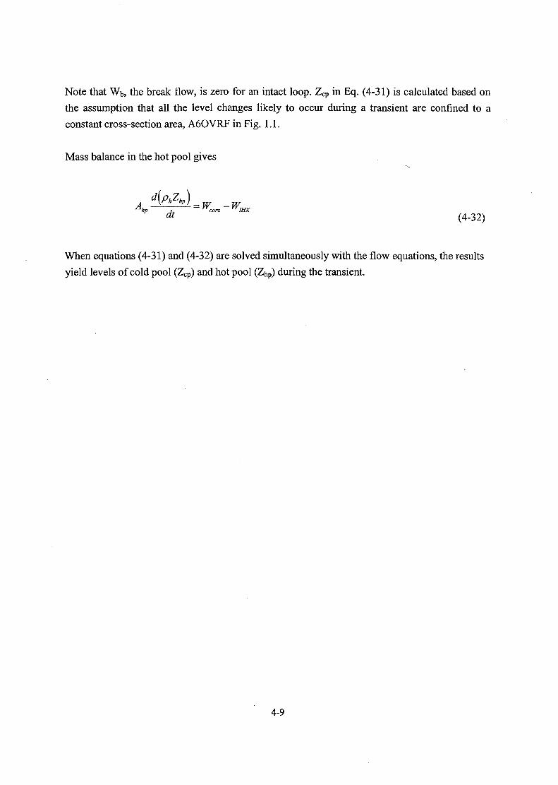
Note that Wb, the break flow, is zero for an intact loop. Zcp in Eq. (4-31) is calculated based on
the assumption that all the level changes likely to occur during a transient are confined to a
constant cross-section area, A60VRF in Fig. 1.1.
Mass balance in the hot pool gives
, , ~ " core " IHXdt (4-32)
When equations (4-31) and (4-32) are solved simultaneously with the flow equations, the results
yield levels of cold pool (Zcp) and hot pool (ZhP) during the transient.
4-9

Ws IntermediateI sodium-in
Intermediatesodium-out
outlet plenum
fixedtubesheet
Primarysodium-in
floatingtubesheet
floatingplenum
PrimaryVVP sodium-out
Fig. 4.1 Flow Paths of KALIMER IHX
4-10

' pB
BypassVolume
t.
tP.OUt
'p .N
outletplenum
p.i+1
1 P.i
primaryflow
inletplenum
inletplenum
1 s.T+1
's.i
secondaryflow
's .1
outletplenum
t ; i's.out
w.
Fig. 4.2 Nodal Diagram for Thermal Balance
4-11

5. ELECTROMAGNETIC PUMP
The electromagnetic (EM) pump is modeled as a component. ITiere are two pump choices
available in the SSC-K code: centrifugal pump which was originally imbedded into the SSC-L,
and an electromagnetic pump. Model description for the centrifugal pump is presented in the
SSC-L code manual. In the SSC-K, an electromagnetic pump model is introduced for the
KALIMER design.
5.1 Pump Models
The KALIMER design contains motor-generators on the primary pumps to extend the
coastdown times of these EM pumps. Combination of EM pumps and motor-generators is
included in SSC-K to handle this configuration. In the current KALIMER design a synchronous
motor is running all of the time during normal operation, but the power to the EM Pump does not
go through the motor as long as the normal pump power is available. If normal pump power is
lost, then the motor becomes a generator, and a switch is thrown automatically to supply voltage
from the motor-generator to the pump. The pump coastdown rate is then determined by the
inertia of the motor. The motor is designed such that it will initially supply 60% of nominal
voltage to the pump. Thus, when normal power is lost and the motor-generator power is switched
on there is a sudden drop in pump head and flow followed by a gradual coastdown.
Pump Head
The pump head is correlated with an expression of the form
H = (V/f)35 hn(W/f) - Lf W2 (5-1)
where
H = H/Hr (5-2)
V=V/Vr (5-3)
5-1

(5-4)
w = w/wr (5-5)
H = pump head
Hr = rated head
V= pump voltage
Vr= rated voltage
f = frequency
fr = rated frequency
w = mass flow rate
wr = rated mass flow rate
Lf = friction loss coefficient and
hn is a head curve correlated as
5
hn (w/f) = 2X- (w/f)j-' (5-6)
with the coefficients ai determined by a least-squares fit to the data.
Pump Efficiency
The pump efficiency, s{, is correlated as
£ =F(V) G(w/f)£* (5-7)
with
G(w/f) = 0.01 if w/f >5
fw/f)3"1' if w/f<5 ( 5"9)
and % = rated efficiency
5-2

Pump Voltage
Before the cut-over to the motor-generator, the pump voltage is assumed to be constant at its
rated value. Also, the frequency is constant at its rated value. Immediately after cut-over, the
voltage drops to a fraction, Vfr, of its initial value. Then the voltage is proportional to the square
of the frequency, so after cut-over the voltage is
V = Vfrf2 (5-10)
where
V f r=0.6 (5-11)
Motor Speed
The equation for the motor speed, s, is
dt Iwhere
r = pump torque
rt = friction loss
I = moment of inertia
Note that the motor speed and the pump frequency are the same:
f=s (5-13)
The pump torque is given by
Hw
where' S/Ps
p = liquid density
The friction loss in the motor is assumed to have the form
5-3
(5-15)
where Lm [s a loss coefficient and Tr, the rated torque.
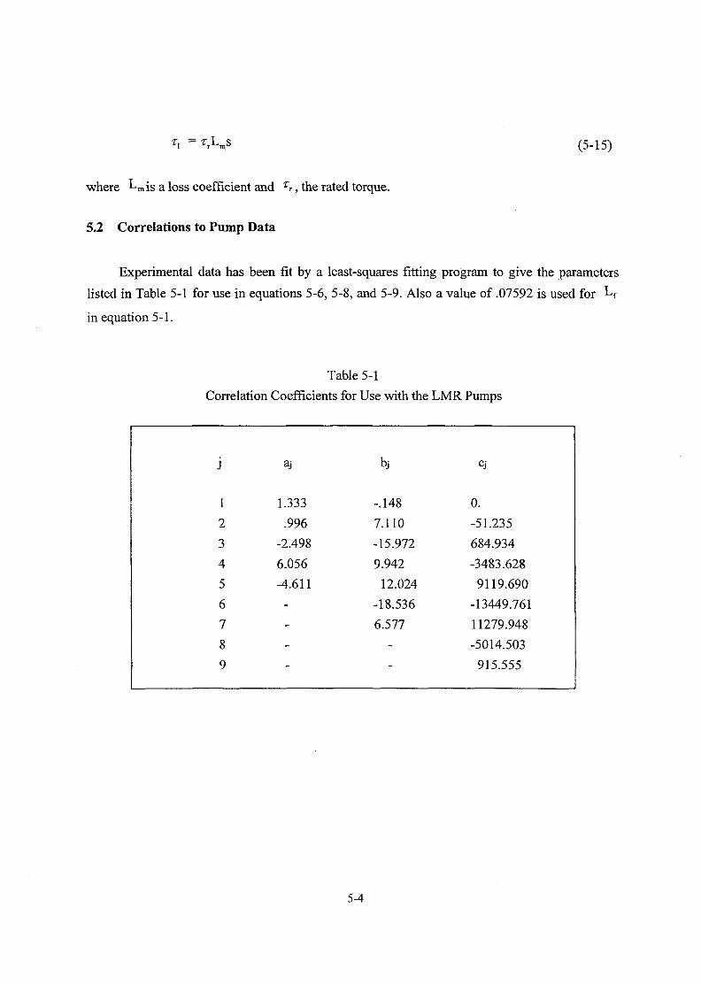
5.2 Correlations to Pump Data
Experimental data has been fit by a least-squares fitting program to give the parameters
listed in Table 5-1 for use in equations 5-6, 5-8, and 5-9. Also a value of .07592 is used for Lf
in equation 5-1.
Table 5-1
Correlation Coefficients for Use with the LMR Pumps
j
1
2
3
4
5
6
7
8
9
aj
1.333
.996
-2.498
6.056
-4.611
-
-
-
-
bj
-.148
7.110
-15.972
9.942
12.024
-18.536
6.577
-
-
Cj
0.
-51.235
684.934
-3483.628
9119.690
-13449.761
11279.948
-5014.503
915.555
5-4

6. PASSIVE DECAY HEAT REMOVAL SYSTEM
6.1 Introduction
PSDRS (Passive Safety Decay Heat Removal System) is a heat removal feature in the
KALIMER design which is characterized to cool the containment outer vessel with atmospheric
air in passive manner. Fig. 6.1 exhibits the schematic of PSDRS. Atmospheric air comes in from
the inlets located top of the containment, and flows down through the annulus gap between the
air divider and the concrete wall. Then, it turns back upward passing through the other annulus
gap between the containment outer surface and the air divider, and, finally, flows out through the
stack with raised temperature by energy gained from cooling of the containment vessel. The air
flow rate is determined from various parameters. Air temperature difference between two
annulus channels, flow path or pressure drop of an orifice placed for flow control, friction
exerted on the surfaces are main parameters affecting the flow rate.
It is important that the air divider should be made of high heat resistance material to
maximize the temperature difference between the inner and outer channels. The gap between the
reactor vessel and the containment vessel is filled with helium gas and thus radiation heat
transfer prevails due to high temperature of these walls.
The significance of PSDRS in the KALIMER design is that it plays a role of the only heat
removal system under total loss of heat sink accident. For this reason, its function is crucial to
prevent the core damage, so that performance analysis as well as realistic modeling of the system
may be a key issue to provide essential knowledge for safety evaluation of the KALIMER design.
6.2 PSDRS Modeling
6.2.1 Basic Assumptions
• Temperature in a wall is represented with one temperature except the air divider as
shown in Fig. 6.1, because the wall thicknesses are thinner than those of gaps between
them by roughly factor of 3 and more over the thermal resistances of the gaps are also
relatively much higher. The air divider, however, is made of material with high thermal
6-1

resistance to reduce conduction across it.
• Air flow is calculated under assumption of quasi steady state, due to much smaller time
constant than those of the walls. Therefore, it is assumed that air temperature varies
axially along the flow channels.
• All walls and air channels are modeled with an equal mesh size which locates the same
elevation in the axial direction. The axial heat conduction is ignored.
6.2.2 Governing Equations
Reactor vessel
The energy balance is set up using heat transfers from sodium or helium gas to the reactor
vessel depending on the sodium level, and between reactor vessel inner and containment outer
surfaces, e.g.
dt
where,
m W i , Cwi : mass and specific heat for the reactor vessel
T N , T W I , T W 2 '• temperatures of coolant or cover gas, reactor vessel, and
containment vessel, respectively
hNWi '• heat transfer coef. between the inner surface of the reactor vessel and the
coolant or cover gas
ANWI , Awi2 '• corresponding heat transfer areas to the heat transfer
coefficients
hWi2 : heat transfer coef. between the reactor vessel and the containment vessel
1 *"" l - + % - (6-2)
The approximation is made that Rwi and RW2 are lumped in with hcvi2, so
Kn = hCyn+Sua(Twl+Tw2)(T^+T^2) (6-3)
6-2

where
(6_4)
£RV £GVI
and
hcvi2 = user-supplied convective heat transfer coefficient, RV to GV
( see 'User Manual')
= emissivity of the reactor vessel wall
- emissivity of the guard vessel inner surface
a = Stefan-Boltzmann Constant
Rwi - GRV / kRv
R\V2 = G G V / kGV
GRV = thickness of the reactor vessel
GGV = thickness of the guard vessel
kRy = thermal conductivity of guard vessel
= thermal conductivity of reactor vessel
Containment vessel
The containment temperature is determined by such terms as heat transfer from the reactor
vessel, convection heat transfer to the up-flowing air, and radiation heat transfer directly to the
inner surface of the air divider. Thus, the balance equation is led to
"" ^~ W "7 T A /m rj-r \ t 7 A /VTI rrt \ • 7 A /m rrt N /" f ^NM7 /** **"~ ri / \ I / ~~ / 1 ~ ~ /7 / \ I / ^~ / I ~4~ ri / \ I I —• / 1 I iW 1 1
£?/ >"12 '2 "'" W2 3 W2<1 Wl" Bi W1
The definitions of the coefficients used in this equation are the same notations as used in
Eq. (6-1). However, Ii2a denotes the heat transfer coefficient between the containment and down-
flowing air, and A2a is the outer surface area of the containment. Tai is temperature of the up-
flowing air. The heat transfer coefficient I123 is given by
1 - % + _ „ . , ' , . , . (6-6)Kn
6-3

Rw2 is neglected, so
^ ^ ) (6-7)
where
*23 = - : —, (6-8)
£GVO
and
SGVO = emissivity of the guard vessel outer surface
SDI = emissivity of the air divider inner surface
Kla 2 hal
again RW2 is neglected, so
Kia = K (6-10)
where the air heat transfer coefficient is
ka = air thermal conductivity
Aoi = hydraulic diameter between the guard vessel and the air divider
Nul = Nusselt number
N. = QRef1 P.M if Re.>Re," ' i i H J i t
C3 if Re,<Re,
R e , = DhaX W" (6-13)Pal MaX
6-4

wa = air flow rate
pal = air density
juai = air viscosity
Pr, = Prandtl number
Ci, C2, C3 = user supplied correlation coefficients
Ci ~ 0.023
C2 ~ 0.8
C3 ~ 3 - 8
Inner and outer surfaces of the air divider
Energy balance equation in the inner and outer surfaces of the air divider are given in
similar manner and thus, it becomes
(6-14)at
(6-15)
Here, T^ represents temprature of the down-flowing air and heat transfer coefficients are given
by
Kia = Kx (6-16)
K-4a = K2 (6-17)
-r- = KS+T- (6-18)
or
{6A9)
6-5

(6-20)
Concrete wall
ATmw5Cw5 T~~ =
at
Where, Tw6 indicates the outer wall temperature of the concrete wall which always remains
constant.
Temperatures of the up- and down-flowing air channels
The balance equations in the up- and down-flowing air channels are given as following
equations, based on the assumptions described earlier.
{TW2 (z) - Ttl (z)) + hwa3Awa3 (TW3 (z) - TA (z)) (6-22)dz
and
AT- Ta2 (z)) + hwa5Awa5 {TW5 (z) - Ta2 (z)) (6-23)
Where, Wa denotes air flow rate and Ca does specific heat of air.
Calculation of air flow rate
Air flow rate is determined from gravitational force balance between down- and up-
flowing air channels, and flow resistance along those channels, e.g.
stack + T,Pa2 U)^j ~ Z Art U)&j ~ Pin (?„ ~ in ) (6"24)j j
and
6-6

( 6 - 2 5 )
where, (Zst - Zjn) is the elevation difference between the inlet and sitack, pa(j) represents air
density in j t h node, and Kor is defined as a form loss coefficient due to the geometry or orifice.
The friction factor is calculated as
Afr Re* if Re > Re,
/ = (6-26)
- ^ if Re<Re,Re J
where
D WRe = Reynolds number = —-—-
Ma A.
jj,a = viscosity
Afr = user-supplied turbulent friction factor coefficient ( see 'User Manual' )
b = user-supplied coefficient (see 'User Manual' )
and
- user-supplied laminar friction factor coefficient
The value of Ret, the Reynolds number for the transition from turbulent to laminar, is calculated
by the code to make the friction factor continuous at the transition point.
Re,* - - ^ (6-27)Re
ori
Re, = ~^- (6-28)Afr
6-7

6.2.3 Solution Method
Schematic of solving the governing equations are presented in Fig. 6.2. Non-linear
differential equations from Eqs. (6-1) to (6-5) are solved using Runge-Kutta Method [6-1], while
Eqs. (6-6) and (6-7) can be solved with typical solution method of linear differential equation, if
the axial wall temperature variations inside a node are ignored. The final solutions of these
ordinary differential equations have a form of
-la)e ' (6-29)
where, i = l,2,which correspond to up- and down-flowing channels, respectively
z> = z~zj (6-30)
T'al = flTW2j + fzTWlj (6-31)
h Ar _ Hw2a •tX
J2 -K2a
(6-32)
fi = 1 - fi (6-33)
h A +h Anw2a •nv/2a T nw3a ^
and above definitions for Ta2 (z1) is similar.
Since the temperature, Tai(0), in Eq. (6-29) is defined at each node interface, so that a node
temperature can be obtained by averaging the temperature profile within the length inside a node.
Thus, the average value is calculated as
6-8

(MS)
For the air temperature calculation, the balance Eqs. (6-24) and (6-25) becomes an
algebraic equation. Thus, air temperature can be calculated straight forward once all coefficients
are known.
6.3 PSDRS Program
Program 'PSDRS' consists of group-wised input variables. User should note that the
sequence of input variables must be consecutive, otherwise there will be a problem to read the
input. Error indication is not enough to find errors in the input lists easily at the present time and
thus users should make sure of the card number and the number of input variables in a card. User
also notes that units of all physical quantities should be given in SI units. Top view of the
KALIMER PSDRS is shown in Fig. 6.3.
6-9

SodiumLevel
L
Hel un
noce
TJ
Ei
0
O"cD
CD>cc.
•
T 3 CD1— COCO CO=3 CD
CD>
qf
4 — •• -pi
Stack
CD•g
Q
ti
r>
7'R2
Inle
Jt
j
N
r
%a,
UJ
_)
N
DELZX
DXRV DXGV
Fig. 6.1 PSDRS Model
6-10

PSDRS UpenFiles
Next Time Step
a- R e
EADIN
ad InputGu<sss Initial Air Temp.
1
- Cal. of SodiumTemp, with Time
yes
AM necessary coef. comprising the equations- Heat transfer coef.- Friction factors- Other coef „ ajs supplied by user through user inputIhvi
RUNGEK
- Solving Equations
TEMPAR
- Air temp, profile through the air channel from inlet
4 >
r
FLWAIR
- Air flow rate calculation
i
EQUr
TNS- Cal. of change rates of variables
yes
Next Iteration
Fig. 6.2 Flowchart of PSDRS Program
6-11

Containmentvessel
Air divider
\ , Reactorvessel
Fig. 6.3 Top View of KALIMER PSDRS
6-12

7. REACTIVITY MODELS
7.1 Introduction
One of the important KALIMER design features is inherent shutdown, which refers to the
tendency of the reactor to transitions to a much lower power level whenever temperatures rise
significantly. There are several reactivity feedbacks important in the inherent shutdown response
for the metal cores, and the core is designed to provide strong, inherent, negative reactivity
feedback with rising temperature. This feature, combined with the heat removal capability of the
PSDRS, makes the KALIMER capable of safely withstanding severe undercooling or overpower
accidents, even without scram.
Only when a major off-normal condition is encountered, combined with a postulated
failure of the Plant Protective System (PPS), can serious accident consequences be predicted.
The inherent shutdown characteristic must be tested against various postulated challenges if it is
to be credited in the licensing arena.
The Super System Code (SSC), developed at BNL for analyzing LMR transients, was
selected as a basis for the development of KALIMER safety analysis code SSC-K. Since the
SSC code was used for the preparation of the PSAR for CRBRP which did not rely on the
passive safety features including reactivity feedback effects, there exist only limited reactivity
models within the code.
The objectives of the current task are (i) to develop a version of SSC-K code which has the
capability of analyzing the inherent safety characteristics of the: metal core, (ii) to gain
experiences of the safety analysis for the unprotected accidents, and (iii) to identify action items
for the further development of the reactivity, component and system models.
Reactivity feedback models have been developed for the SSC-K code in order to account
for the effects due to Doppler, sodium density/void, fuel axial expansion, core radial expansion
and control rod driveline expansion. These models will be used to establish a working version of
the SSC-K code which is essential for the development of component and system models as the
7-1

KALIMER design progresses.
Attempts have been made for the application of the models in order to gain insight on the
inherent safety characteristic under the postulated unprotected accident conditions. Reactivity
models developed are not for actually generating a safety analysis results of KALIMER design
but for the preparation of the further modeling efforts when the reactivity coefficients can be
generated through a detailed neutronics calculation.
Efforts also have been made for the identification of the limitations and of the further
modeling needs for the current version of the code through the preliminary safety analysis.
7.2 Reactor Kinetics
Nuclear reactor kinetics models predict the time behavior of the neutron population in a
reactor core induced by changes in reactor multiplication. Diffusion model is capable of
describing the time behavior of a nuclear reactor, provided the effects of delayed neutrons are
included. However, such a model is too detailed for practical implementation in reactor kinetics
analysis due to excessive computation requirements.
Point reactor kinetics approximations can be used more effectively for fast reactors than for
thermal reactors because the neutron flux is more nearly separable in space and time for fast
reactors. Fast reactor safety codes to date have therefore generally employed point kinetics,
however, the reactivity feedback terms due to reactor temperature variations and material motion
generally contain spatial effects.
7.2.1 Point Kintetics Equations
The total heat generation per unit volume p (r, t) is given as
P (r, 0 = Pf (r, t) + Pd (r, t) (7-1)
where pf {?, o is the heat generation rate per unit volume due to nuclear fission and pd £ o is
the decay heat generation rate per unit volume.
7-2

While the spatial power distribution in a reactor core is of interest in the steady-state
operation of the plant, the temporal power distribution is of utmost importance in day-to-day
plant operation, reactor stability studies, and safety. The time-dependent portion of the fission
power contribution is calculated by solving the space-averaged, one-energy group reactor
kinetics equations. The one-energy group assumption is reasonable, particularly for a fast reactor.
The space-averaged model is quite adequate since the core of an O»1FBR responds, due to the
relative smallness of the core and the large neutron migration area, more uniformly than a light
water reactor core to changes in reactivity.
The point-kinetics equations may be expressed as
dt A M (7_2)
L = L N - 4C, {i = 1,2,..6) (7-3)at A
where
N = neutron density (neutrons/m3),
t - time(s),
p = reactivity (Ak/k),
f3T = effective delayed neutron fraction =
A = prompt neutron generation time(s)
= prompt neutron lifetime / multiplication factor k,/I. = decay constnant for the i-th delayed neutron group(s'),Ct = density of the i-th effective delayed neutron precursor
(precursors /m3),
PT = effective delayed neutron fraction for the i-the group.
It should be noted that for a particular isotopic composition of a reactor, a single set of X.t and
P( values is obtained and utilized in the kinetics equations.
It is convenient to rewrite Eqs. (7-2) and (7-3) in a normalized form by defining the normalized
neutron density, n(t) and concentration of the i-th group precursor, ct{t), as
7-3
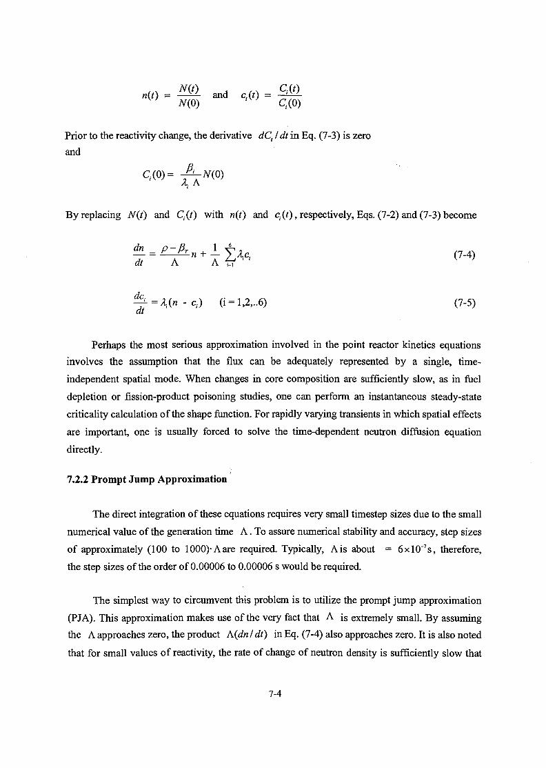
N(t) , , , C.n(t) = —-— and cXt) = -
N(0) Cand cXt)
N(0) C,(0)
Prior to the reactivity change, the derivative dCi I dt in Eq. (7-3) is zero
and
Cf(0)= -^TN(0)\ A
By replacing N(t) and Ct(t) with n(t) and c,.(f), respectively, Eqs. (7-2) and (7-3) become
( 7 .4 )dt A A t i " '
<^-=X(n-c.) (i = l,2,..6) (7-5)dt
Perhaps the most serious approximation involved in the point reactor kinetics equations
involves the assumption that the flux can be adequately represented by a single, time-
independent spatial mode. When changes in core composition are sufficiently slow, as in fuel
depletion or fission-product poisoning studies, one can perform an instantaneous steady-state
criticality calculation of the shape function. For rapidly varying transients in which spatial effects
are important, one is usually forced to solve the time-dependent neutron diffusion equation
directly.
7.2.2 Prompt Jump Approximation
The direct integration of these equations requires very small timestep sizes due to the small
numerical value of the generation time A. To assure numerical stability and accuracy, step sizes
of approximately (100 to 1000)-A are required. Typically, A is about = 6xlO"7s, therefore,
the step sizes of the order of 0.00006 to 0.00006 s would be required.
The simplest way to circumvent this problem is to utilize the prompt jump approximation
(PJA). This approximation makes use of the very fact that A is extremely small. By assuming
the A approaches zero, the product A{dn I dt) in Eq. (7-4) also approaches zero. It is also noted
that for small values of reactivity, the rate of change of neutron density is sufficiently slow that
7-4
dnldt is negligible compared to the two terms on the right hand side of Eq. (7-4). Thus, n
may be directly solved for as
7i= - i - 2>U (7-6)PT-P I
This means that any disturbance in the reactivity (p) will be instantaneously reflected in the
neutron density n jumps immediately to some initial level dependent on the size of the
reactivity insertion.
Since dn I dt was assumed to be zero, the PJA is in excellent agreement (to within < 0.1 %)
with the exact solution for values of P less than +50 cents. It should be noted that this
approximation gets even closer to the exact solution when the prompt neutron generation time is
smaller.
The main drawback of using the PJA is the fact that agreement to the exact solution
diminishes as p approaches f5T. It can be seen from Eq. (7-6) that n is discontinuous at
p = jBT. To provide for these cases where p approaches flT (or more conservatively, when
p > 50 cents) an optional numerical method is included in SSC-K which solves the equations
exactly.
7.2.3 Kagnove Method
To provide an exact solution to Eqs. (7-4) and (7-5), without integrating them directly, the
method proposed by Kaganove was used in SSC. Here, Eqs. (7-5) are solved for c, in terms of
dct I dt and substituted into Eq. (7-4) such that
^L = El 1 yA^Ei (7 7\dt A A lfXi dt ' K '
The assumption is then made that over any integration step (At), the normalized power (n) andreactivity (p) may be represented by second-order polynomials. Thus,
n(t) = n0 + n/ + nf ; 0 < t < At, (7-8)
p(t) = p0 + Plt + pf ; 0 < / < At, (7-9)
7-5
where
n0 = value of n at the end of previous timestep9
p0 = value of/? at the end of previous timestep
and «,, n2, /?,, p2 are constants to be evaluated
Eq. (7-5) is now integrated in a straightforward manner:
Then
c,(t) = cme-Xi> + Ze-*'[e^n(ju)dM (7-10)
where
Making use of Eq. (7-8), Eq. (7-10) becomes
(7-11)- 2 ( 1 - e"*)
Likewise, Eq. (7-7) becomes
7i(0 - 11(0) - 1
Upon substituting Eqs. (7-8) and (7-9) into Equation (7-12), one obtains
7-6

1 t2 t3 t2
= —(ponot + p o n , - + p 0 n 2 - + p x n 0 -
e, - (7-13)
1 '
The boundary conditions are then imposed that integral Eq. (7-13) be satisfied at the midpoint
and end of the step (i.e., at t - At/2t and t = At).
Thus, Eq. (7-13) yields two equations in the unknown «, and n2. With the assumption that
during any given timestep, the power and reactivity are functions of time only (i.e., decoupled),
the solution in SSC will proceed as follows.
(a) using the predicted value of reactivity at t = At and two previous values, the two
constants px and p2 in Eq. (7-9) are calculated;
(b) using Eq. (7-13) solved at At 12 and At, the constants «, and n2 are calculated;
(c) the predicted power may then be calculated using Eq. (7-8).
7.3 Reactivity Effects
Values for reactivity effects are required both for transient safety analysis and for control
requirements during normal operation. Reactivity effects of importance in fast reactor design and
safety include the Doppler effect, effects of sodium density changes or loss of sodium, effects of
dimensional changes in core geometry, and long-term reactivity loss from fuel burnup.
The total reactivity at a given time, t , is the sum of as applied reactivity, pa(t) e.g.,
control rod movement, plus the sum of the various reactivity feedback contributions,
P(O = PM) + 2>,(0 (7-14)
As indicated in Fig. 7.1, the total reactivity is then incorporated into the point-kinetics
model and used in the evaluation of the normalized time dependent factor for the fission and
gamma heating. It should also be noted that the reactivity effects are inherently space-dependent.
This is not only due to the fact that the temperatures vary spatially, but even for the same
7-7

temperatures the magnitude of the effect will depend on the location within the reactor. Since the
point-kinetics equations suppress any spatial dependence, an appropriately weighted spatial
integration of the evaluated local reactivity feedback effects must be performed.
In the following sections, models for various reactivity feedback effects are discussed. For
the reactivity effects of dimensional changes in core geometry, fuel axial expansion, core radial
expansion and control rod driveline expansion are considered.
Due to the unavailability of reactivity coefficients for KALIMER core designs at the
present time, test runs have been performed for the SSC-K representation of the KALIMER for
the preliminary verification of the reactivity models and for the better understanding of the
reactor response under unprotected accident conditions.
7.3.1 Doppler Effect
It is important to have a prompt negative reactivity feedback that reverses a power transient
if the reactor becomes prompt critical. Mechanical action by control rods is too slow after
prompt criticality is reached. A prompt negative feedback is particularly important for fast
reactors because two mechanisms, fuel compaction and sodium loss, have the potential to make
the reactor superprompt critical.
The Doppler effect is the most important and reliable prompt negative reactivity effect in
current thermal and fast reactor designs which utilize high fertile U238 material concentrations.
Probably one of the better understood reactivity phenomena, the Doppler effect is due to the
increased kinetic motion of the fuel atoms, as measured by an increase in fuel temperature,
resulting in the broadening of cross-section resonances and increased resonance absorption.
The Doppler reactivity comes predominantly from the capture of low-energy neutrons.
Ceramic-fueled reactors, due to the presence of oxygen or carbon in the fuel, have a soft enough
neutron spectrum to have a large Doppler effect. The high density metal reactor, having no
moderator in the fuel matrix, yields the hard neutron spectrum, and the flux in the principal
Doppler resonance region (0.1 - 10 keV) is appreciably less than for the ceramic fueled reactor.
Consequently, both oxide and carbide fueled fast reactors possess much higher Doppler
7-8

coefficients than metal fueled reactors. This represents one of the important advantages of
ceramic over metal fuel.
7.3.1.1 Hard Spectrum Case
The Doppler coefficient, dk/dT, is defined as the change in multiplication factor, k,
associated wit an arbitrary change in the absolute fuel temperature, T. For a reactor with hard
neutron spectrum, such as a metal-fueled fast reactor, the theory for the effective Doppler cross
section indicates that dk I dT should vary as l/T3'2, i.e.,
f • £where a001" is the Doppler constant which is independent of temperature.
Eq. (7-15) may be integrated to yield
where To and T represent two different fuel temperatures and k0 and k are the resulting
multiplication factors. Rigorously, reactivity is defined as
k - 1
and changes in reactivity, Ap, as
k - k,Ap = p - p0 =
0
kk, 0
For small reactivity changes, the Doppler effect is of the order of KT4.With k « 1,
A/7 « k - k0
7-9

and the change in reactivity due to the Doppler effect ApDOP, can be written as
A DOP o DOP / *• \ y*T -t T \
Ap = 2 a (-r= - -;=-) (7-17)
By definition, the reactivities are referenced to zero at steady state conditions, that is, ko=\
and p0 = 0, and the Doppler reactivity can be rewritten as
DOP ry DOPf 1 J
(
DOP _ ry ^DOPf 1 _J_\ / 7 i m
p ( ^ ' ^ } ( }
This is equation may be applied locally or regionally depending on how the temperatures and
Doppler constant are defined. Specifically, in discrete notation, the local Doppler reactivity,
pST = 2 <P(-X= - -7=) (7-19)V-'OJX V-v*
where
K = index of fuel channel
J = index of the axial level along the fuel channel
a™p = the node-weighted Doppler constant for position JK
T0JK = the reference fuel temperature at position JK
TJK = the effective local temperature at position JK
The effective fuel temperature can be taken to be the volume-averaged fuel temperature which is
defined as
Z V T'UK* UK
( 7 ' 2 0 )
UK1
where V K is the fuel volume is channel K, axial slice J, between radial mesh / and / - I ,
7-10
and TUK is the local fuel temperature at this position. Figures 7.3 and 7.4 show the SSC-K
representations of reactor core subassemblies and radial node within a fuel rod, respectively.
It should be noted that the Doppler constant in Eq. (7-19) is shown to be a space-dependent
variable. Although a°°p will be a constant with respect to fuel temperature, there will be spatial
variations due to different fuel types (e.g., enrichment, pin size, volume fractions of structural
material, coolant, and fuel) and different sodium density. In the pres;ent model, a%"> will be a
space-dependent parameter supplied by the user. Thus, the first concern relating to fuel type can
be directly addressed.
The sodium density dependences is actually a neutron spectrum dependence- the harder the
spectrum, the smaller the Doppler effect since there are less neutrons in the resonance range. The
less sodium present, owing to density decreases or voids, implies a harder spectrum. To treat this
effect, an effective isothermal sodium void fraction, X1]*, is defined
* NayNa _ PoJK " PjK c-i /•> -I \
POM
where Na is the local, time-dependent sodium density at position jg, and Na is the localPJK POJK
reference sodium density. Thus, if RD0P and nD0P are the Doppler constants with and withoutPJK *"*«
sodium present, respectively, then the net Doppler constant can be approximated by
<" = K°Pa - X%) + Q?XZ; (7-22)
To obtain an overall Doppler reactivity, pDOP, for use in the point - Kinetics equation, asummation of Eq. (7-19). must be performed. Thus
PDOP = 5> 7 = 2j> 7 (-JL - * ) (7-23)^1 ^1JK JK.
The value of the Doppler constants, ft™1" and Q^°p for each position JK, must be supplied
by the user in units of reactivity Ak I k for that mesh.
7.3.1.2 Soft Spectrum Case
7-11

Since the Doppler coefficient is found to vary with \IT in a oxide-fueled fst reactor, this
coefficient an be defined as
dk a°°F
where aD0P is a temperature independent Doppler constant.
For a uniform change in fuel temperature from To and T, Eq. (7-24) may be integrated to yield
k -ko = aD0P\n^-) (7-25)
where k and k0 are resulting multiplication factors.
For small reactivity changes with k « 1, the Doppler reactivity effect can be calculated as
pD0P = „«*!„(!.) (7.26)
which can be applied locally and rewritten as
p™ = a?ln&-) (7-27)•*QJK
To obtain an overall Doppler reactivity, DOP , for use in the point kinetics equation, a
summation of Eq. (7-27) must be performed. Thus,
'1«(|S (7-28)
where of™ is also defined by Eq. (7-22).
Input requirements for the calculation of Doppler reactivity are /3j°p and Qj°p in
7-12

7.3.1.3 Other Models
ARIES code also calculates the Doppler reactivity coefficient by the Eq. (7-28) with
temperatures in Rankines.
SASSYS code calculates the Doppler feedback reactivity, pD0P, based on summation,
over fuel axial nodes in all channels, the contribution for a node which is based on a mass
weighted average fuel temperature, as well as on how much fuel and sodium are currently
present in the node:
-DOP
PjKJK
T (7"29)
whereWJK — Doppler weighting factor for axial node J in chann el K.
normalized for each channelpoor = Doppler coefficient for channel K with all sodium present
QDOP — rjOppier coefficient for channel K with no sodium present
mf = fuel mass of the node JK
mJfK
0 — initial steady-state mass of fuel in the node JK
p = average density of sodium in the node JK
p = initial steady-state density of sodium in the node JK
TJK = average temperature of fuel in the node JK
TJK0 = initial steady-state temperature of fuel in the node JK
The valves for the unvoided and voided Doppler coefficient, p°op and Q.™p, for each channel,
as well as the weighting factors are supplied by the user, based on neutronics calculations or
experimental measurements.
7-13

7.3.2 Sodium Density Effect
The loss of sodium from a large fast reactor can result in a large positive reactivity effect.
Sodium might be expelled from the core in the unlikely event of an unprotected transient, in
which sodium boiling results from undercooling the reactor. This condition presents an important
safety problem for an LMFBR, a problem not present in thermal reactors.
The sodium loss reactivity effect is exceedingly space-dependent. Sodium loss from the
center of the core yields a highly positive reactivity effect, and sodium loss from near the edge
gives a negative effect. The density decreases affect the reactivity of the reactor through two
competing effects: increased leakage, which adds negative reactivity and is important away from
the center of the core, and spectral hardening due to a decrease in the macroscopic sodium
scattering cross-section which adds positive reactivity. The net effect depends primarily upon the
location in the reactor.
In modeling this effect, both sodium density changes and voiding can be treated in a
similar fashion. Basically, what is required along with the spatial sodium density distribution is a
table of space-dependent sodium reactivity worths. The sodium density will be determined
internally by SSC from knowledge of the sodium temperature distribution. However, the
reactivity worths are user supplied.
There are several ways to present this reactivity effect depending on the form in which the
reactivity worth data are known. For application in SSC, the following equation, which can treat
either sodium density or voiding reactivity effects, is used
(7-30)
where pNa is the overall sodium void reactivity coefficient for use in the point-kinetics equation,
fiJK is the sodium reactivity worth in axial slice J, channel K, in units of reactivity per unit mass
of sodium voided in segment JK, and is defined as
MJK = ( / £ - PTK) V% (7-31)
7-14

where p"°K is the local sodium density at reference temperature, p% is the local average,
time-dependent sodium density and V% is the local coolant volume in segment JK.
Input requirements for the calculation of sodium void reactivity according to the Eq. (7-30) are
the mesh weighted sodium void reactivity coefficients pjK in &k/k P e r kg of sodium
effectively voided.
The sodium void reactivity may also be calculated based on the changes in sodium temperatures
as
PNa = ZAr * W " O (7-32)JK
where j3JK is the sodium void reactivity coefficient in Ak/k perK
Tj° is the sodium temperature at axial node J of channel K
and T"°K is the initial steady state sodium temperature at axial node J of channel K.
The ARIES code computers the sodium void reactivity as
NaPJK * ( r* - O (7-33)JK
where aNa is the sodium volumetric expansion coefficient in "
PM is the sodium void reactivity coefficient in
and T!ia and T!1" are sodium temperatures in °p
The sodium voiding model in SASSYS-1 and SAS4A is a multiple-bubble slug ejection
model. The main purposes of this model are to predict the rate and! extent of voiding for the
voiding reactivity calculations and to predict the heat removal from the cladding surface after the
onset of voiding for the fuel and cladding temperature calculations.
7.3.3 Axial Expansion Effect
A role of axial expansion of fuel in the normal solid fuel pin geometry is to provide a
prompt negative reactivity feedback at the start of a power transient. This mechanism is the
principal prompt negative feedback available in a metal-fueled fast reactor. Doppler feedback is
7-15

also available for the metal-fueled system, but it is relatively small due to the hard neutron
spectrum. For a ceramic-fueled reactor, lack of structural integrity due to cracking in high burnup
fuel renders the axial expansion mechanism somewhat unreliable so that more dependence is
placed on the Doppler effect for a prompt negative feedback.
The fuel axial expansion increases the core height as temperatures rise, and changes the
reactivity of the system by increasing the neutron leakage. The result is a rapid negative
feedback contribution from an increase in fuel temperature, or a rapid positive feedback in
response to a decrease in fuel temperature. The axial leakage changes only a little with axial fuel
expansion, but the radial leakage does increase, thereby producing a negative reactivity effect,
which can be shown as follows.
The criticality factor can be expressed as
where k is the product of the criticality factor for an infinite reactor, k , and the fast neutron
nonleakage probability, 6-B2M2 . For a cylindrical core,
k - kme
Now let us suppose that fuel expands axially as a result of increasing fuel temperature during the
rise to full power or in a power transient. Radial fuel expansion may increase fuel pin diameters
slightly but will have relatively little effect on radial expansion of the core. Bulk radial core
expansion is governed primarily by the structure and hence, the coolant temperatures, together
with the influence of the radial restraint system. Hence, the primary core expansion from
increased fuel temperature is in the axial direction.
According to conventional reactor theory, the migration area varies with transport and total
cross sections as
7-16
where ^ tr and ^ t are effective transport and total cross sections that provide the correct
nonleakage probability. / / is the number density offuel and structure atoms.
For a fixed number offuel and structure atoms,
N oc — ocV R2Z
where y = volume of the core
R = core radius
and z = core height
Thus M2 « R4Z2» DUt n o w Z is the only dimension in p that changes during axial fuel
expansion. Hence, the criticality factor can be presented in terms of the only parameter that is
varying, z , a s
k = kj***'* e^*1* = kae-c> ec>* (7-36)
This result indicates that the axial leakage does not change with axial fuel expansion, but that the
radial leakage does increase, thereby producing a negative reactivity effect.
An upper limit to the magnitude of this effect is obtained if iit is assumed that the fuel
pellets are free to move within the cladding. However, the actual mechanisms for expansion are
difficult to model, especially for ceramic fuel. Fuel pellet cracking or friction between the pellet
surface and inner clad wall will reduce the expansion significantly. On the other hand, if the fuel
pellets are not stacked in perfect contact within the clad, then there may be negative fuel
expansion if the fuel pellets settle. Physics calculations for CRBRP indicate a maximum overall
reactivity of -.18 <t /mil offuel axial expansion. The range of this effect is quoted to be +.025 (£
/mil to -.18 0 /mil owing to the uncertainties involved in the expansion mechanism.
The lack of strong Doppler coefficient for metal fuels, which is caused by the characteristic
hard neutron spectrum, has historically been compensated for by the presence of a reliable axial
expansion coefficient. The ternary U-Pu-Zr fuel swells out to contact the HT9 cladding material
7-17

around 2-3% atom bumup. After the fuel-clad lockup occurs, the fuel thermally expands
according to the thermal expansion of the clad material. This is because the strength of metal fuel
is very limited, and thus its expansion is dominated by the clad expansion. Experiments have
shown that a 4% axial elongation is possible in the 1.9 to 5.3% burnup range.
The reactivity effect due to the thermal expansion usually decreases with the increase in
reactor core size.
There are three models in the SSC-K code available for the evaluation of fuel axial
reactivity coefficient. Free fuel expansion model, which gives the upper limit to the axial
expansion reactivity, assumes that the fuel expands freely in the axial direction, and fuel -
cladding contact is ignored. Uncertainties in the axial reactivity coefficient are accounted for by
the uncertainty factor, and this is the original model present in the SSC-L code.
Force balance controlled expansion model assumes that the fuel is in contact with the clad,
which is the most likely state for the metal-fueled core since the fuel is in an unlocked state only
briefly. The fuel elongation is calculated by using an average strain, weighted with Young's
modulus.
Another model is the one for ARIES code, which is based upon the fuel and clad
temperature variations. Axial expansion may be optionally calculated based upon clad
temperatures for conservative analyses of postulated accident conditions.
The simple model of the SASSYS code is based on a few assumptions. During the
transient, if the cladding expands faster than the fuel, then the fuel-cladding gap opens, and the
fuel can expand freely in the axial direction. If the fuel expands faster than the cladding, then the
fuel binds with the cladding, and the axial expansion is determined by balancing the axial forces
between the fuel and cladding.
7.3.3.1 Free Fuel Expansion Model
The reactivity due to fuel axial expansion, p** is based on a model which parallels the
treatment of sodium density reactivity effects:
7-18

JK (7-37)
where CJK is the user-supplied fuel reactivity worth in axial slice J, channel K, in units of
reactivity, Ak/k, per unit mass of fuel effectively voided from segment JK, and N*x is the
effective mass of fuel voided in segment JK.
An expression for the evaluation of N JK is derived based on the logic that as the fuel
temperature increases, the fuel expands axially according to
a(TJK - T0JK)]Zt (7-38)
where a is the linear fuel expansion coefficient in units of cm I cm K and TJK is volume -
averaged fuel temperature. To conserve mass, an axial increase in the fuel length implies a
decrease in the fuel density pJK, which can be expressed as
or
— P
P OM - P JK= P OJK l + a(TJK-T0JK)JK M OJK > .
(7-39)
(7-40)
The difference in density times the original fuel volume, K , will give the amount of fuel
voided from location, JK, NJK,
= (POv n I <x(TJK-T0JK)VOJK yOJK + a(TJK-T0JK)JK * OJK ' _
(7-41)
The effective amount of fuel voided from location JK, N' , and the resulting net reactivity
effect associated with fuel axial expansion are given as
N' - eNJKJK JK
(7-42)
7-19

P = e L C* N« (7-43>JK
where e is a user-supplied constant that accounts for the fact that the present model does not
account for the uncertainties associated with the mode of fuel expansion and does not explicitly
evaluate the increase in reactivity because the fuel that was calculated to be voided from location
JK actually causes a net increase in axial fuel height, reducing leakage. A recommended upper
limit for e is given to be 0.3 for oxide fuels.
For the calculation of fuel axial expansion reactivity, a user needs to supply CJK, the fuel
reactivity worth in axial slice J, channel K, in units of reactivity (Ak/k) per kg of fuel effectively
voided from segment JK.
7.3.3.2 Force Balance Controlled Expansion Model
This model assumes that the fuel is locked and expands with clad. The reactivity worth is
determined from the difference between the initial fuel length and the elongated length at any
given time.
The axial expansion reactivity coefficient dkldz is defined as
dk a**— = (7-44)dz z
where aM ^s a n a x ia l expansion constant in units of A& . This equation may be integrated to
yield
pM = aM In ( - ) (7-45)zo
In discrete notation
P" = UP f = Z < M—) (7-46)* K Z
where
Z0k
7-20
a™K - an axial expansion constant for channel K in units of Ak
z* = the elongated axial length of channel K
z°* = the axial length of channel K at reference temperature To
By definition, the effective strain ( A # / J ) of K-th channel, 4 , can be expressed as
_ z k - z ok
and rewritten as
(7-47)
(7-48)
The effective strain of channel K can be calculated by using an average strain, weighted with
Young's modulus as
Z 0 *
r>Jk
, (7-49)
where£ = index of channelj = index of the axial position along the channel
z0Jlc = the axial length of segment JK at reference temperatureY = Young's modulus
p^ = Nominal cross-sectional area
and subscripts/and c represent fuel and clad, respectively.
7-21

The strains of fuel and clad can be obtained from
= <*' ' T/JK) (7-50)
& = a' {TJK - T;JK) . (7-51)
where
af = the thermal expansion coefficient of the fuel
of = the thermal expansion coefficient of the clad
TjK = the average temperature of fuel in segment JK
TjK — the average temperature of clad in segment JK
To = the reference temperature
Input requirements for this model are as follows:
af = the thermal expansion coefficient of the fuel
ac = the thermal expansion coefficient of the cladY = Young's modulus for fuel and clad
a^K = axial expansion constant in units of Ak
af and of are currently calculated in subroutine TEXP, while Y and a** are provided in
subroutine GR0W5T of SSC-K.
7.3.3.3 Other Models
ARIES code adopts a fuel-clad expansion model as
PM - Z [ aCP« W""* - TN\JK) + <xFPx (TFJK - T\M) ] (7-52)
JK
where ac = the cladding linear expansion coefficient in °F"'
aF = the fuel linear expansion coefficient in °F"'
pcM = the cladding axial expansion reactivity coefficient in Ak
p^ — the fuel axial expansion reactivity coefficient in Ak
Axial fuel expansion can also be calculated based on cladding temperature as
7-22
5> N°0JKJK
- TN°0JK) (7-53)
Usually, Eq. (7-52) is used when analyzing undercooling events and Eq. (7-53) is used for
conservative analyses of transient overpower events.
It is assumed in SASSYS code that before the start of the transient, a combination of fuel
cracking, fuel re-structuring, and stress relaxation cause the gap between the fuel and the
cladding to close, but there is little contact force between the fuel and cladding. During the
transient, if the cladding expands faster than the fuel, then the fuel-c ladding gap opens, and the
fuel can expand freely in the axial direction. If the fuel expands faster than the cladding, then the
fuel binds with the cladding, and the axial expansion is determined by balancing the axial forces
between the fuel and cladding. Slip between fuel and cladding is ignored in this case.
The reactivity calculation is based on the user-supplied local fuel reactivity worth, in units
of reactivity, Ak/k, per unit mass of fuel effectively voided from the segment.
7.3.4 Radial Expansion Effect
7.3.4.1 SSC-K Model
Radial fuel expansion due to increasing fuel temperature may increase fuel pin diameters
slightly but will have relatively little effect on radial expansion of the core. Bulk radial core
expansion is governed primarily by the structure and, hence, the coolant temperatures, together
with the influence of the radial restraint system.
The core assemblies are held by their nosepieces in the receptacles, and by the load pads
near the top of the assemblies which are surrounded by a core restraint ring attached to the core
barrel, as shown in Fig. 7.6. The separation of the assemblies is maintained by an intermediate
plane of load pads at an elevation above the active core. The intermediate load pads above the
core are not restrained by a former ring attached to the core barrel. Thus, the core assemblies are
free to bow as dictated by temperature differences and their metallurgical condition.
The radial dimension of the core is largely determined by the assembly spacing. This spacing is
7-23
determined by the grid plate below the core and by two sets of load pads above the core.
The redial expansion reactivity coefficient, dkl dr, can be defined as
(7-54)
where aR is a radial expansion constant in units of Ak. This equation may be integrated toyield
p* = a" ln( - ) (7-55)rro
where
r = the radial dimension of core at transient temeprature
r0 = the initial steady-state radial dimension of core
By definition, the effective strain ( A/ / / ) , E,, can be expressed as
r -r°
and rewritten as
7 I + <Thus
p R = aR ln(l + £) (7-56)
The coefficients a*, for radial expansion effect, were calculated assuming a uniform
increase over the core radius. However, the above core load pad (ACLP) responds to core exit
sodium temperature while the grid plate (GP) responds to the core inlet temperature. This causes
non-uniform expansion and the worth for each component must be weighted. From geometrical
considerations, the split is W^ for ACLP and W^ for GP. Hence, the radial expansion
reactivity can be calculated as
p* = ccR l#i(l + W^ 4 > + WGP ZGP) (7-57)
7-24

where
WLP = geometrical weighting factor for the ACLP
WGP = geometrical weighting factor for the GP
The strain of the A C L P can be calculated as
5>' £ (7-58)K
where
K = index of the fuel channel
NK = number of subassemblies in K-th channel across core radius layout
as shown in Fig. 7.6
££ = strain (Ar/r ) for ACLP of channel K
The strains of the ACLP and the GP for channel K can be obtained as
C = a^T^ - T0K) (7-59)
ZGP = aGP(TGP - 7 f ) (7-60)
where
dy, = the thermal expansion coefficient of the A C L P
aGP = the thermal expansion coefficient of the GP
T* = the initial steady state temperature of the A C L P at K-th channel
T* — the volume-averaged temperature of the A C L P at K-th channelavg
T° = the initial steady state temperature of the GP' 0
TGP = the temperature of the GP.
7.3.4.2 Other Models
The ARIES code computes the thermal expansion reactivity coefficient as a sum of
contributions from the fuel axial expansion, core radial expansion, and bowing effects. A Global
radial expansion reactivity coefficient is utilized for the core radial expansion effect.
7-25

Two radial expansion feedback models are available in SASSYS-1: a simple model and a
more detailed model.
The simple model assumes that
1. The reactivity feedback is determined solely by thermal expansions of the grid support
plate and load pad region, with all regions having the same thermal expansion coefficient.
2. The displacement of the core mid-plane is sufficient to estimate the reactivity feedback
from the radial core expansion.
3. All of the subassembly load pads are in contact throughout the transients.
The equations actually used in SASSYS are
fi" = Crc [AT, + *y£ (ATSLP - AT;)] (7-61)
whereCrc = coefficient, $/K
AT, = changes in coolant inlet temperature
XMC = distance from nozzle support point to core mid-place
XMC = distance from nozzle support point to above ACLP
ATSU, = changes in average structure temperature at ACLP
This model was not explicitly set up to account for subassembly bowing or flowering of the core,
but the user can set arbitrary values for Crc and XMC/ XMC. Therefore, if the bowing reactivity
effect is proportional to ATSLP or the ATSLP - AT,., then bowing reactivity can be accounted for
by adjusting Crc and XMC/XAC.
The simple model, however, does not explicitly account for subassembly bowing, and is
not capable of calculating changes in core loading conditions during the course of a transient.
In a more detailed model, rather than maintaining the cylindrical shape associated with a uniform
core dilation, an axial profile of core radius is calculated. During a transient, the changes in the
axial profile are used in conjunction with a worth curve for radial core expansion, such as the
one obtained with NUB0W-3D code, to yield the reactivity feedback.
7-26

7.3.5 Control Rod Driveline Expansion Effect
Thermal expansion of the drives due to a rise in core outlet temperature will cause the
control rods to be inserted further into the core, providing a negative reactivity component. On
the other hand, if the control rod drives are supported on the vessel head*- and if the core is
supported by the vessel walls, then heating the vessel walls will either lower the core or raise the
control rod drive supports, leading to a positive reactivity component. The effect of vessel
expansion needs to be analyzed carefully for the KALIMER design which adopts PSDRS.
A simple one node treatment is used for calculating the temperature of the control rod
drives.
( 7"6 2 )
where
Mc mass of the control rod drives, kg
specific heat of the control rod drives, J/kgK
control rod drive temperature, K
time, sec
heat transfer coefficient between coolant and control rod drive, W/m2 K
heat transfer area, m2
coolant temperature in the upper plenum region, K
In finite difference equation form, the above equation becomes
or
1 +
(7-63>
(7-64)
where
d. -M
7-27

Z° = T* {1 + a TB{t) + H(f) Zj(t) TAt)cr cr *- cr B v J TT fj\ A ^ s
H(t)
Z} (t) = penetration height into upper mixing plenum of average core exit flow, m
H(t) = height of sodium in upper mixing plenum above top of core, m
TA (t) = temperature of sodium in upper mixing zone of upper outlet plenum, K
TB (t) = temperature of sodium in lower mixing zone of upper outlet plenum, K
For calculation of T£(t), two-zone mixing model of SSC-K is used during transient.
However, a single-zone perfect mixing model is used at steady state, and the control rod drives
and coolant in the upper plenum region are assumed to be in thermal equilibrium. That is,
7 ; ( 0 ) = TX •
where 2J is the vessel sodium outlet temperature in K.
At steady state, the length of control rod drive can be calculated as
Z : = Z? {1 + ^ ( ^ ( 0 ) ) * (7;(0) - T?)} (7-65)
where
Zi = steady state length of control rod drive immersed in sodium, m
= reference length of control rod drive immersed in sodium, m
~ reference height of sodium in upper mixing plenum above top of core, m
= linear coefficient of thermal expansion for control rod drive, m/m K
= reference control rod drive temperature, K
Expansion of the control rod drive from the steady state length can be expressed as
AZ^ = Z: * acr(Tr(t)) * {(Tcr(t) - O (7-66)
For vessel expansion,
MS; ^ = M . OZ - TJ (7-67)
7-28

where
Mvs = mass of the reactor vessel, kg
CJ = specific heat of the reactor vessel, J/kgK
7^ = temperature of the reactor vessel, K
t - time, sec
hvs = heat transfer coefficient between the coolant and the reactor vessel , W / m 2 K
Avs = heat transfer area, m 2
T*a = coolant temperature adjacent to the reactor vessel, K
Above equation can be solved for the reactor vessel temperature 7^ us
r . W • ' • ( ' ' 0 + 1 T O (7.68)1 + a
vs
where
d =MS:
= mean coolant temperature in upper region of bypass, K
The vessel height at steady state can be calculated as
Zl =Z'*{\ + aJTJO)) (Tvs(0) - T?)} (7-69)
where
Zv° = reactor vessel height at steady state, m
Zrvf = reference vessel height, m
~ reference sodium level from bottom of reactor vessel, m
a^ = linear coefficient of thermal expansion for reactor vessel, m/m K
Trjf = reference reactor vessel temperature, K
Expansion of the reactor vessel from the steady state height can be expressed as
7-29

= z: * a.(r.(/) * {r (o - o (7-70)
Thus the effective control rod driveline expansion can be calculated as
(7-71)
Reactivity for control rod driveline expansion is calculated as
pCR=CCRAZ (7-72)
where CCR is the user-supplied coefficient for control rod driveline expansion in Ak/k per m.
Control rod driveline expansion model of the SASSYS-1 code is similar to the one described
above.
7.4 Input Requirements for Reactivity Feedback Models
For the generation of the reactivity coefficients by the core design group of the KALIMER
design team, descriptions of each model with the definition of the reactivity coefficient are
summarized below. Discussions with the core design group for the SSC-K reactivity feedback
models will be based on the following descriptions which will be included in the Design Data
Request for the Safety Analysis.
7.4.1 Doppler Effect
Reactivity coefficients need to be provided for one of the models described below or for
any other model suggested by the core design.
Model 1
y DOP V"1 _ DOP ^ Y 1 ^ DOP r * \ tn T>\KP = L,P JK = 22^a JK ( I - ~l=) (7"73)
JK JK ^1 0JK yjj JK
DOP _ ftDOPs-i yNa\ , r)DOP yNa ( n - .^"•JK ~ PjK V-XJK) + ilJK XJK (7-74)
where
7-30

K
J
XJK
- index of the fuel channel
= index of the axial level along the fuel channel= the initial steady state fuel temperature at position JK
= the effective local temperature at position JK
= an effective isothermal sodium void fraction
Input Requirements:
f3j°p - Doppler coefficient with Na present for node JK, AkI k
Q.Dj°p = Doppler coefficient without Na present for node JK, Ak/k
Typically, twelve axial nodes are used for the entire length of the fuel rod: two for lower blanket
or shielding, six for active fuel, and four for upper gas plenum.
Model 2
DOP
1OJK
P = PJK (1 " XJK ) + " j r XJK
Input Requirements:
= Doppler coefficient with Na present for node JK, Ak I k
= Doppler coefficient without Na present for node JK, Ak/k
Model 3
(7-75)
(7-76)
nDOP X * _ DOP
P = 2a P JKJK
p JK0 iM:o
(7-77)
where
mf = fuel mass of the node JK
7-31

mf0 = initial steady-state mass of fuel in the node JK
pJK = average density of sodium in the node JK
pJK0 = initial steady-state density of sodium in the node JK
TJX = average temperature of fuel in the node JK
TJK0 = initial steady-state temperature of fuel in the node JK
Input Requirements:
WJK = Doppler weighting factor for node JK, normalized for each channel
J3j°p = Doppler coefficient for channel K with all sodium present
Q.Dj°F = Doppler coefficient for channel K with no sodium present
7.4.2 Sodium Density Effect
Reactivity coefficients need to be provided for one of the models described below or for
any other model suggested by the core design.
Model 1
PJK MJK (7-78)JK
where MJK is the effective mass of sodium voided in the segment JK.
Input Requirements:
fiJK = sodium void reactivity coefficient for axial slice J of channel
Model 2
pNa = 1 4 * ft? - C ) (7-79)JK
7-32

Input Requirements:
/3JK = sodium void reactivity coefficient for the axial slice J of channel K,
Ak/k/K
Model 3
pN° = J > N a J3JK * (r* - O (7-80)
JK
Input Requirements:
aNa = sodium volumetric expansion coefficient in °F-1
j3M - sodium void reactivity coefficient for the node JK in Ak/k
7.4.3 Axial Expansion Effect
Reactivity coefficients need to be provided for one of the models described below or for
any other model suggested by the core design.
Model 1
(7-81)
where NJK is the mass of fuel voided from segment JK.
Input Requirements:
e = a user-supplied constant that accounts for the uncertainties associated with
the mode of fuel expansion
7-33

= fuel reactivity worth in axial slice, J, channel K, in Ak/k per unit mass
fuel effectively voided from segment JK
Model 2
_ K - /_,-» f ln (—) (7-82)K K Zok
where
zK = the elongated axial fuel length of channel K
zok - the axial fuel length of channel K at reference temperature To
Input Requirements:
af = an axial expansion reactivity coefficient for channel K in units of Ak
Model 3
pM = ^[acp^(TNajK- TN"0JK) + aFpFK(TFjK- TFOJK)] (7-83)
JK
Input Requirements:
ac = the cladding linear expansion coefficient in K 1
aF — the fuel linear expansion coefficient in K1
PjK = the cladding axial expansion reactivity coefficient in Ak
pFK = the fuel axial expansion reactivity coefficient in Ak
1.4.4 Radial E x p a n s i o n Effect
Reactivity coefficients need to be provided for one of the models described below or for
any other model suggested by the core design.
Model 1
p R = aR I n (1 + WLP ZLP + WGP %CP) (7-84)
7-34

where %LP and %GP are the strains of Above Core Load Pad (ACLP) and Grid Plate (GP),
respectively.
Input Requirements:
aR = the radial expansion reactivity coefficient in units of Ak
WLP = geometrical weighting factor for the ACLP
Wap = geometrical weighting factor for the GP
Model 2
pa = CJATin + j ^ (ATSLP - A?;)] (7-85)
where
A7Tn = changes in coolant inlet temperature
XMC = distance from GP to core mid-place
XAC = distance from GP to ACLP
/±TSLP = changes in average structure temperature at ACLP
Input Requirements:
Crc — the radial expansion reactivity coefficient, $/K
7.4.5 Control Rod Driveline Expansion Effect
Reactivity coefficients need to be provided for the model descnibed below or for any other
model suggested by the core design.
pCR = Cc*(AZcr - AZJ (7-86)
where AZcr and AZ^ are the changes in CRDL and reactor vessel height, respectively.
Input Requirements:
CCR = CRDL expansion reactivity coefficient in Ak/k per m
7-35
7.5 Flowcharts
Figure 7.9 shows the modularized structure of the reactivity feedback subroutines of SSC-
K. Each box contains subroutine names, which are underlined, and a brief description of their
functions. All subroutines shown in the figure are implemented into the SSCTK code except for
GEM5T which will be developed for the analysis of gas expansion modules in the core.
7.6 GEM Model
Gas Expansion Modules (GEMs) are added to KALIMER core in order to supplement the
negative reactivity feedback that develops once the primary pump has been tripped. When the
pumps trip and the pressure drops, the sodium within the GEMs at the active core elevation is
displaced by Helium gas, thus increasing the leakage of neutrons from the core and subtracting
about [TBD] cents of reactivity, assuming all 6 GEMs function properly.
The GEM is essentially an empty hexagonal cross section duct, sealed at the top, open at
the bottom and connected to the high pressure in the inlet plenum of the core as shown in Fig.
7.7. When the pumps are at full flow, the plenum pressure compresses the gas in the GEM cavity.
When the flow decreases, the trapped Helium expands and drops the sodium level into the core
region. As a result, fewer neutrons are scattered back into the core region. The reactivity effect
increases as the gas expands into the core and remains constant once the gas liquid interface
drops below the core region.
The objective of this study is to develop a simple model for the analysis of the reactivity
effects introduced by the GEM, and to identify the areas of further improvement.
7.6.1 Current GEM Model
In order to calculate the sodium level in the GEM, the following equations are solved. As
shown in Fig. 7.8, the total length of GEM is occupied by the Helium gas and primary sodium as
K + ht = h, (7-87)
7-36

where
hg = axial length of Helium gas in GEM, m
h, = axial length of sodium in GEM, m
ht = total axial length of GEM, m
Since there is no sodium flow through the GEM, the pressure of sodium at the core inlet plenum
can be expressed as
Pg+pgh,=P, (7-88)
where
Pg = GEM gas pressure, Pa
P; = pressure of sodium at core inlet plenum, Pa
= (pressure of sodium at bottom of core)
- (gravitational pressure drop along the orifice inlet zone)
p = average density of sodium in GEM, kg/m3
g = gravity, m/s2
The equation of state for ideal gas is applied for the Helium gas in the GEM as
where
A = cross sectional area of GEM, m2
Mg = massofHeliumgasinGEM, kg
Wg = melecular weight of Helium gas, kg/mole
R = universal gas constant, J/K mole
Tg = temperature of Helium gas in GEM, K
Unknowns in the Eqs. (7-87) to (7-89) are h , A/5and P

The average density of sodium in GEM, p, is assumed to be the density corresponding to the
average temperature of sodium in adjacent subassemblies.
The gas temperature, Tg, closely follows the GEM duct temperature which is determined
by considering the heat transfer between the neighboring subassemblies and the GEM. For
simplicity, the gas temperature is assumed to be the average of the temperatures of duct walls of
adjacent subassemblies.
Equations (7-87) to (7-89) can be rearranged to give a quadratic equation for the axial
length of Helium gas in GEM, hg, which is calculated at each time step. The worth of the GEMs
when the sodium level is equal to, or greater than, the top of the core is zero. When the level
reaches the bottom of the core, the maximum worth of GEM is inserted. Intermediate values of
reactivity are interpolated linearly from the sodium level in the GEMs.
Subroutine GEM5T of SSC-K code has been developed to calculate the level of sodium
inside GEM and the negative reactivity inserted. GEM5T is called by REAC5T which drives the
overall reactivity calculations.
7.6.2 GEM Model Improvement
A GEM model, which will be used for the analysis of LOF accident, has been developed
for SSC-K code, and reasonable results have been obtained through test runs. Due to the lack of
detailed design data, including dimensions, sodium levels at various operating regimes, mass of
Helium gas inside GEM, and GEM reactivity worth as a function of sodium level, a simplified
model was developed first in order to study the effectiveness of GEM under LOF accident
conditions.
Following are the items which need further work for the current GEM model:
• Currently the sodium density inside the GEM is assumed to be the axial average of the
neighboring channels. Sensitivity study is needed to investigate the effect of sodium
density on the sodium level. If needed, the GEM model will be modified so that the axial
sodium density is calculated considering inter-assembly heat transfer.
7-38

The temperature of the GEM gas is assumed to the average of the structural temperature
of neighboring channels. Improvement of the current GEM model can be achieved by
calculating the GEM gas temperature as
where
cp = Specific heat of GEM gas, J/kg*K
Q = Heat from conduction from neighboring channels, watts
In addition to the model improvement described above, more detailed design data are
essential for the analysis of GEM effect.
- GEM worth curve : sodium level vs reactivity
- Sodium level at various operating regimes
- Mass of GEM gas
The effect of primary pump coastdown can be investigated and generate the
requirements for the coastdown.
7-39

Total Reactivity
Feedback Reactivity
Fission Power CalculationsBy Point Kinetics
Applied Reactivity
Total Reactor Power
Decay Power
Doppler Effect
Sodium Density Effect
Fuel Axial ExpansionEffect
Core Radial ExpansionEffect
CRDL ExpansionEffect
Fuel Temperatures
Sodium Temperatures
Fuel and CladTemperatures
GP and ACLPTemperatures
CRDL and RVTemperatures
Fig. 7.1 Overall Scheme for Calculating Total Reactor Core Power
7-40

CoreFormer
Ring
Top of CoreLoad Pad
(TCLP)
Above CoreLoad Pad
(ACLP)
Active Core
^ Control Rod DriveLine Reactivity
Axial ExpansionReactivity G a s Expansion
/ Module (GEM)
Grid Plate
Radial ExpansionReactivity
SodiumReactivity
DopplerReactivity
Fig. 7.2 Components of Reactivity Feedback Effect
7-41

Q Driver Fuel 46
!p Internal Blanket 18
^ Radial Blanket 72
^ Control Rod
(•) OSS
( GEM
j I Reflector
^ B,C Shield
^ 1 IVS
^ Shield
6
1
6
48
54
54
72
Total 379
Fig. 7.3 Schematic of Core Layout for Reactivity Model Development
7-42

Driver Internal RadialFuel Blanket Blanket Control Reflector Shield
IVSHotFuel
UpperFissionGas
Plenum
ActiveRegion
LowerShielding
¥H . "
!==*.-;,
a? '
i11
Fig. 7.4 SSC-K Representation of Core Subassemblies
7-43

Fuel Clad Coolant Structure
'2
O
' 3
O
R,Cl
R,
T
Gap
'NF
O
'CO
Fig. 7.5 SSC-K Representation of Fuel Rod
7-44

Control Rod DriveLine
Control | i ;
Rod
Gas Plena
ActiveCore
Core Former Ring
GridPlate
Fig. 7.6 Typical Core Restarint System
7-45

TOPLOADPAD
SHIELD
ABOVECORELOADPAD
INLETSECTION
GEM OPERARTION SCHEME
Na
CORE
Na
PUMP ON PUMP OFF
Fig. 7.7 GEM Operation Scheme
7-46

Z6BCOR
Z6BCOR
Z6UFGP
Z6UBLK
Z6AFUL
Z6LBLK
Z6LFGP
Z6INZ
Fig. 7.8 Schematic for GEM Model Development
7-47

REAC5T
Total Reactivity
PRMT5T
Prompt NeutronFission Power
Applied Reactivity(Scram/Control Rods)
Doppler Effect
Sodium Density Effect
GEM5TGas Expansion
Module
GR0W5TFuel Axial Expansion
Effect
P0W5T
TotalReactor Power
Decay Power
Core Radial ExpansionEffect
CRDL5TCRDL Expansion
Effect
Fuel Temperatures
Sodium Temperatures
Sodium Pressure
Fuel and CladTemperatures
GP and ACLPTemperatures
CRDL and RVTemperatures
Fig. 7.9 Flow Diagram of Reactivity Feedback Calculation for SSC-K
7-48

8. CONSTITUTIVE LAWS AND CORRELATIONS
A number of constitutive laws and correlations are required in order to execute the SSC
code. T collection or part of these data may be overwritten by the user. This section describes
collections of data that have he approach taken is based on providing the best available data into
the code. The entire been incorporated so far. All of the correlations and numerical values used
are in SI units.
8.1 Constitutive Laws
The required thermo-physical and transport properties for all of the materials of interest are
provided for in the form of correlations. Reasonable values for the coefficients in these
correlations are provided in SI units. These values may be changed by the user through input
cards. Various constitutive laws are grouped according to materials.
8.1.1 SSC-L Properties
8.1.1.1 Core and Blanket Fuel
Thermal Conductivity (W/m K)
The thermal conductivity of mixed oxide [8-1] core (UO2-2O w/o PU02) and blanket (oxide)
materials is given by the following relation:
K(T,P)= k»(l-p) \—+i,f (8-1)l + (k + kP)Pk+kT 3
Where typical values for ko, ki, k2, k3, 1Q and ks are noted in Table 8-1, and P is the fractionalporosity (=1- fractional density).
Specific Heat Capacity (J/ kg K)
8-1

The specific heat capacity of mixed-oxide [8-2] core and blanket materials is given by the
following relations:
for T<T, (8-2)
T2-Tx
for T,<T<T2 (8-3)
= c4+c5T for r>71 (8-4)
where values of various parameters are noted in Table 8-1, and
and
+ c 7f] (8-5)
(8-6)
Table 8-1
Parameters on Fuel Thermal Conductivity and Specific Heat Correlations
Parameterkok,k2k3k4k5PCoCi
c2c3c4c5c6TiT2
Fuel material113.30.780.029356.600* 10-13
110input194.3191.3557*10"3
-9.3301 *10-7
2.4482* 10"10
502.951003020.03060.0
Blanket material113.30.780.029356.60* 10"13
110input194.3191.3557*10-3
-9.3301*10'7
2.4482*10-10
502.951003020.03060.0
8-2
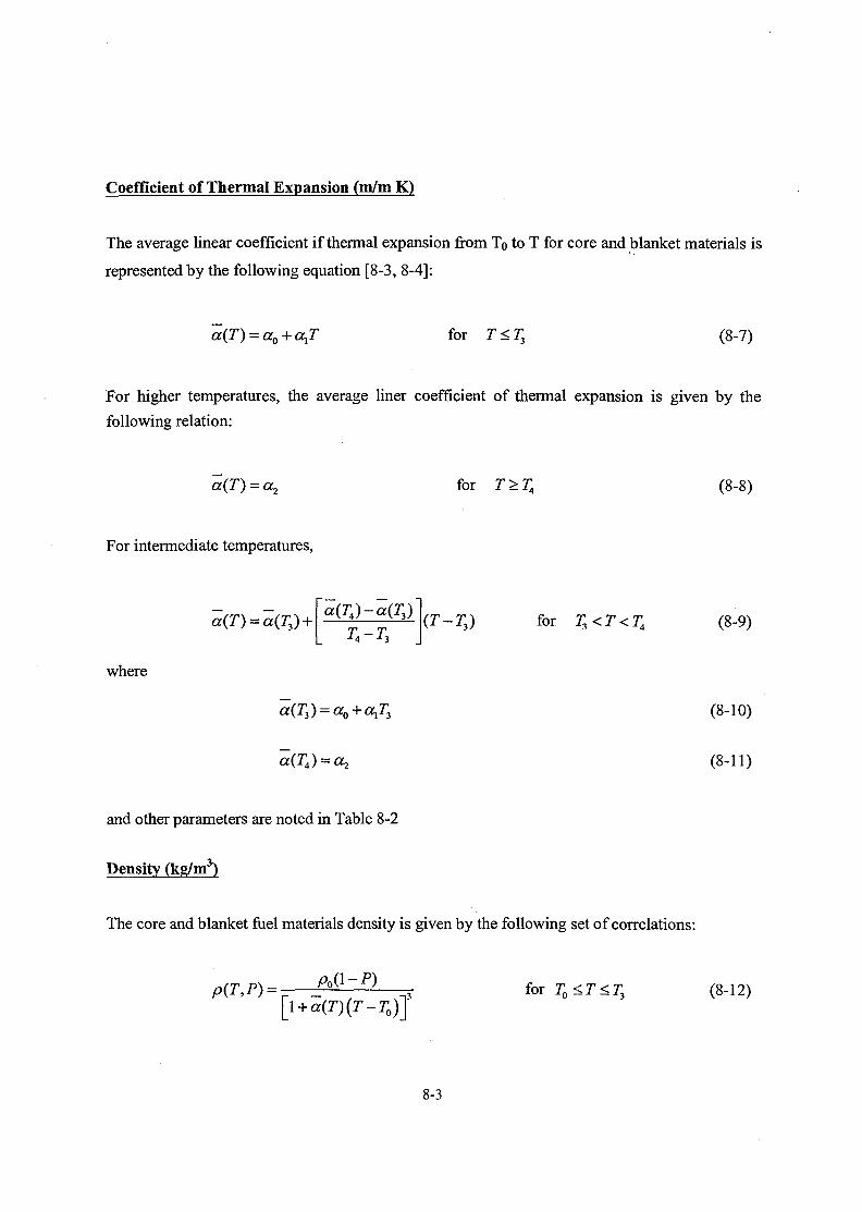
Coefficient of Thermal Expansion (m/m K)
The average linear coefficient if thermal expansion from To to T for core and blanket materials is
represented by the following equation [8-3, 8-4]:
~a(T) = ao + axT for T<T3 (8-7)
For higher temperatures, the average liner coefficient of thermal expansion is given by the
following relation:
a(T) = a2 for T>T4 (8-8)
For intermediate temperatures,
"«(r4)-«(r,)'L ^ for r3<r<7; (g_9)4 ^3 J
where
(8-10)
a2 (8-11)
and other parameters are noted in Table 8-2
Density (kg/m3)
The core and blanket fuel materials density is given by the following set of correlations:
/*T,F) = r ™ \ ' .3 fori + a(T)(T-T0)]
8-3
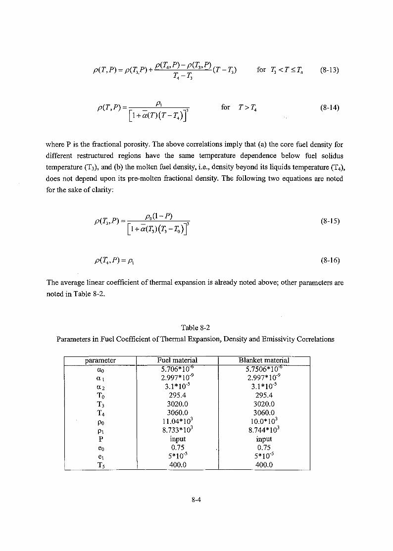
p(T, P) = p(T3P) - T3) for T3<T<T4 (8-13)
Al + a(T)(T-T4)]
for T>T4 (8-14)
where P is the fractional porosity. The above correlations imply that (a) the core fuel density for
different restructured regions have the same temperature dependence below fuel solidus
temperature (T3), and (b) the molten fuel density, i.e., density beyond its liquids temperature (T4),
does not depend upon its pre-molten fractional density. The following two equations are noted
for the sake of clarity:
P(T3,P) = —-dl + a(T3)(T3-TQ)]
(8-15)
(8-16)
The average linear coefficient of thermal expansion is already noted above; other parameters are
noted in Table 8-2.
Table 8-2
Parameters in Fuel Coefficient of Thermal Expansion, Density and Emissivity Correlations
parameteraoa i
a 2
ToT3
T4
PoPiPeoeiT5
Fuel material5.706*10"°2.997*10"9
3.1*10"5
295.43020.03060.0
11.04*103
8.733* 103
input0.75
5*10'5
400.0
Blanket material5.7506*10"°2.997* 10"9
3.1*10"5
295.43020.03060.0
10.0*103
8.744* 103
input0.75
5*10"5
400.0
8-4

Emissivity (Dimensionless)
The core and blanket material emissivity [8-5] is given by the following correlations:
e = eQ for T<T5. (8-17)
and
e = ea+e,(T-T5) for T>T5 (8-18)
where eo, ei and T5 are given in Table 8-2 .
8.1.1.2 Cladding and Structural Materials
For stainless steel, the default material for cladding and structure, the thermal conductivity
(W/m-k) [8-6], specific heat (J/kg K) [8-6], and the average linear coefficient of thermal
expansion (m/m-K) [8-7], are represented by polynomial fits of data. These equations, for
temperatures up to melting point, are given by the following:
2+k3Ti • (8-19)
and (8-20)
a(T) = ao+ axT + a2T2 (8-21)
where values for various parameters for both cladding and structural materials are noted in Table
8-3. The structural or cladding material density is related to the average thermal coefficient of
linear expansion as follows:
p(T)Po [l + a(T)(T-T0)]
8-5
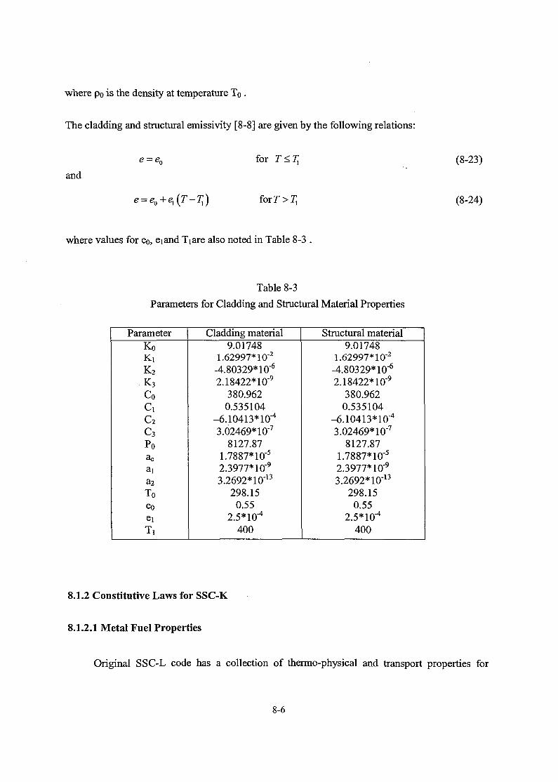
where po is the density at temperature To .
The cladding and structural emissivity [8-8] are given by the following relations:
for T<T,and
(8-23)
(8-24)
where values for eo, eiand Tiare also noted in Table 8-3 .
Table 8-3
Parameters for Cladding and Structural Material Properties
ParameterKoK,K2
K3
Coc,c2c3Poacaia2
ToeoeiT,
Cladding material9.01748
1.62997* 10"2
-4.80329* 10"6
2.18422*10"9
380.9620.535104
-6.10413*!©"4
3.02469*10-7
8127.871.7887*10"5
2.3977* 10"9
3.2692*10-°298.15
0.552.S*!©-4
400
Structural material9.01748
1.62997* 10"2
-4.80329*™-6
2.18422*10"9
380.9620.535104
-6.10413*™"4
3.02469* 10'7
8127.871.7887*10-5
2.3977* 10-9
3.2692* 10-13
298.150.55
2.5*10~4
400
8.1.2 Constitutive Laws for SSC-K
8.1.2.1 Metal Fuel Properties
Original SSC-L code has a collection of thermo-physical and transport properties for
8-6

selected materials, however, additional properties are necessary for materials which will be used
for KALIMER design. Table shows properties which are provided in the SSC-K code:
E denotes properties which are in the original code, and N denotes newly added properties.
K, W/m K
Cp, J/kg K
a,m/mK
p, kg/m3
E
UO2-2O w/oPuO2
E
E
E
E
E
U-Zr-Pu
N
N
N
N
Stainlesssteel
E
E
E
E
E
HT9
N
N
N
ModifiedSubroutines
gama5s,gama5tstem5sprop5t
alfa5s,prop5tprop5t
Detailed description of changes is summarized below:
• Equations with fixed coefficients are inserted in the subroutines, and input parameters
are dummies.
• For general material types, input requirements and block data need to be modified.
Thermal Conductivity
Material(ID)
Blanket(40-49)
Fuel(50-59)
Clad(60-69)
Structure(70-79)
InputParameter
C4K0 ~ C4K^ C 5 K F
C5K0 ~ C5K^ C 5 K F
C6K0 ~ C6K^C6KF
C7K0 ~ C7K^•C7KF
Subroutine
CALC7R
Thermal ConductivityParameter
COND5K
COND5K
COND6K
COND7K
SubroutineGAMA5SGAMA5TSTEM5SGAMA5SGAMA5TSTEM5SGAMA5SGAMA5TSTEM5SGAMA5TSTEM5S
Changes
MOX -> U-Pu-Z
MOX -> U-Pu-Z
SS •» HT9
SS -» HT9
8-7
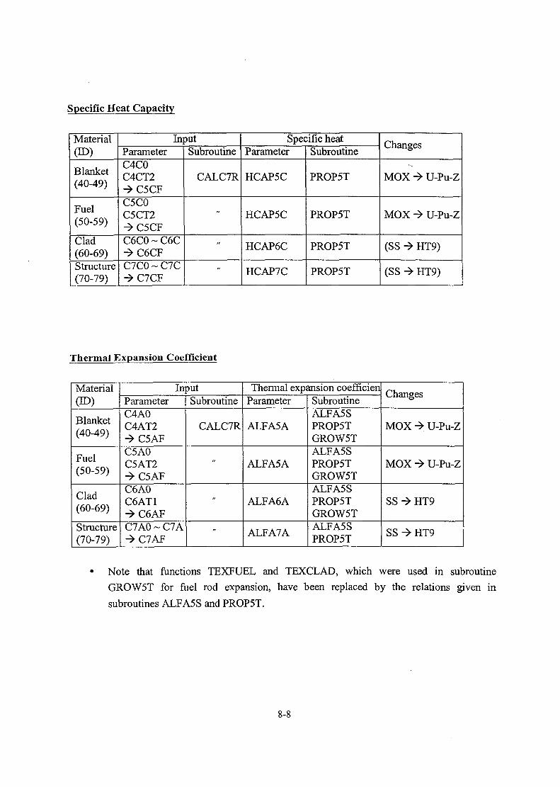
Specific Heat Capacity
Material(ID)
Blanket(40-49)
Fuel(50-59)
Clad(60-69)Structure(70-79)
InputParameterC4C0C4CT2->C5CFC5C0C5CT2^•C5CFC6C0-C6C->C6CFC7C0 ~ C7C->C7CF
Subroutine
CALC7R
"
"
"
Specific heatParameter
HCAP5C
HCAP5C
HCAP6C
HCAP7C
Subroutine
PROP5T
PROP5T
PROP5T
PROP5T
Changes
MOX -> U-Pu-Z
MOX •* U-Pu-Z
(SS -> HT9)
(SS -» HT9)
Thermal Expansion Coefficient
Material(ID)
Blanket(40-49)
Fuel(50-59)
Clad(60-69)
Structure(70-79)
InputParameterC4A0C4AT2->C5AFC5A0C5AT2^ C 5 A FC6A0C6AT1->C6AFC7A0 ~ C7A->C7AF
Subroutine
CALC7R
»
"
"
Thermal expansion coefficienParameter
ALFA5A
ALFA5A
ALFA6A
ALFA7A
SubroutineALFA5SPROP5TGROW5TALFA5SPROP5TGROW5TALFA5SPROP5TGROW5TALFA5SPROP5T
Changes
MOX •* U-Pu-Z
MOX -> U-Pu-Z
SS -» HT9
SS -» HT9
Note that functions TEXFUEL and TEXCLAD, which were used in subroutine
GROW5T for fuel rod expansion, have been replaced by the relations given in
subroutines ALFA5S and PROP5T.
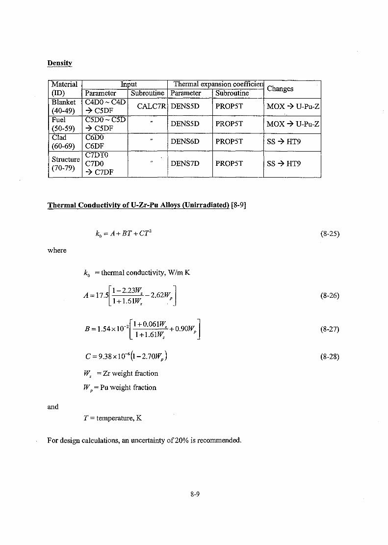
Density
Material(ID)Blanket(40-49)Fuel(50-59)Clad(60-69)
Structure(70-79)
InputParameterC4D0 ~ C4D->C5DFC5D0 ~ C5D->C5DFC6D0C6DFC7DT0C7D0->C7DF
Subroutine
CALC7R
"
"
Thermal expansion coefficienParameter
DENS5D
DENS5D
DENS6D
DENS7D
Subroutine
PROP5T
PROP5T
PROP5T
PROP5T
Changes
MOX -> U-Pu-Z
MOX -> U-Pu-Z
SS -> HT9
SS -> HT9
Thermal Conductivity off U-Zr-Pu Alloys (Unirradiated) [8-9]
where
k0 = thermal conductivity, W/m K
= 17.5+ 1.6WP1
= 1.54x10- 2
1 + 1.61PF1 p
and
C = 9.38xlOH5(l-2.7O0;)
Wz = Zr weight fraction
Wp — Pu weight fraction
T = temperature, K
For design calculations, an uncertainty of 20% is recommended.
(8-25)
(8-26)
(8-27)
(8-28)
8-9

Thermal Conductivity of U-Zr-Pu Alloys (Irradiated) [8-9]
bk (8-29)where P — porosity fraction referenced to initial fuel volume and J3=1.7
The minimum value of fp is taken as 0.5 ±0.1 and the long-time value is 0.7 ±0.1 to reflect the
influence of sodium logging and fuel hot pressing. For design purposes an uncertainty of ± 32%
is recommended after porosity interlinkage.
Specific Heat of U-Zr-Pu Alloys [8-101
6 2 ] ( 3 ) (8-30)
where
4 . 3 5 9 +0.05812T +
= specific heat capacity
temperature, K
1.086 xlO6J"2
forU-10wt%
]/(238xlO"3)
Zr, J/kg K
Linear Thermal Expansion Coefficient of U-Zr-Pu Alloys [8-11]
where
a, = linear thermal expansion coefficient of U-10 wt % Zr, m/m K
— = 0.01 x[-0.424+ (1.658 xlO"3r)-(1.052 xlO"6r2) +(1.115 xlO'9r3)] (8-32)A)
for 293<r<900^.
8-10
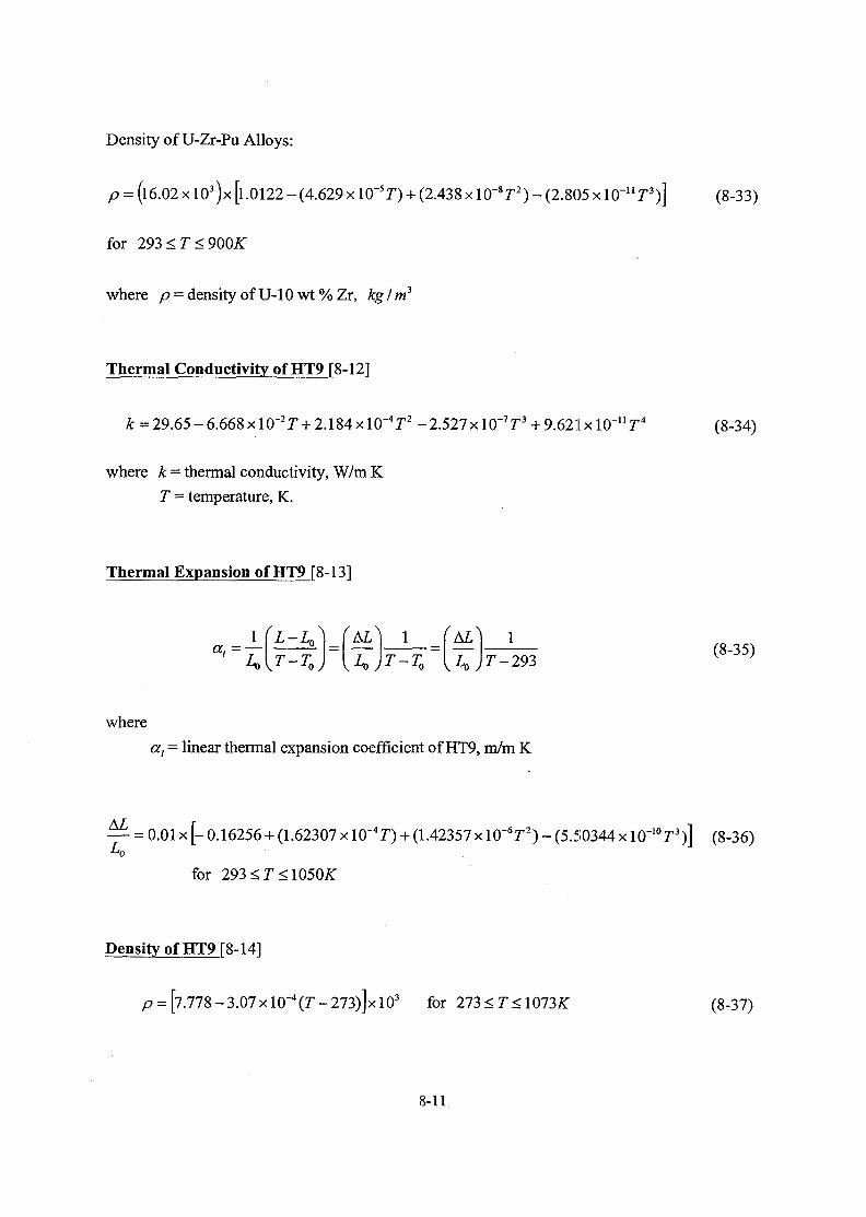
Density of U-Zr-Pu Alloys:
= (l6.02xl03)x [l.O122-(4.629 xlO"5r) +(2.438 xlO"8r2)-(2.805
for 293 < 7 < 900^
where p = density of U-10 wt % Zr, kg In?
Thermal Conductivity of HT9 F8-121
(8-33)
A: = 29.65 - 6.668 x 10~2 r + 2.184 xlO-4r2-2.527 xlO-7r3+9.62 l x l O - u r
where k = thermal conductivity, W/m K
T - temperature, K.
(8-34)
Thermal Expansion of HT9 \8-13]
,8(8"
wherecct = linear thermal expansion coefficient of HT9, m/m K
.42357xl0~6r2)-(5.50344xl0"10r3)] (8-36)
for 293<r<1050/<:
Density of HT9T8-14]
p = [7.778-3.07x 10^(7-273)]xlO3 for 273<r<1073^ (8-37)
8-11
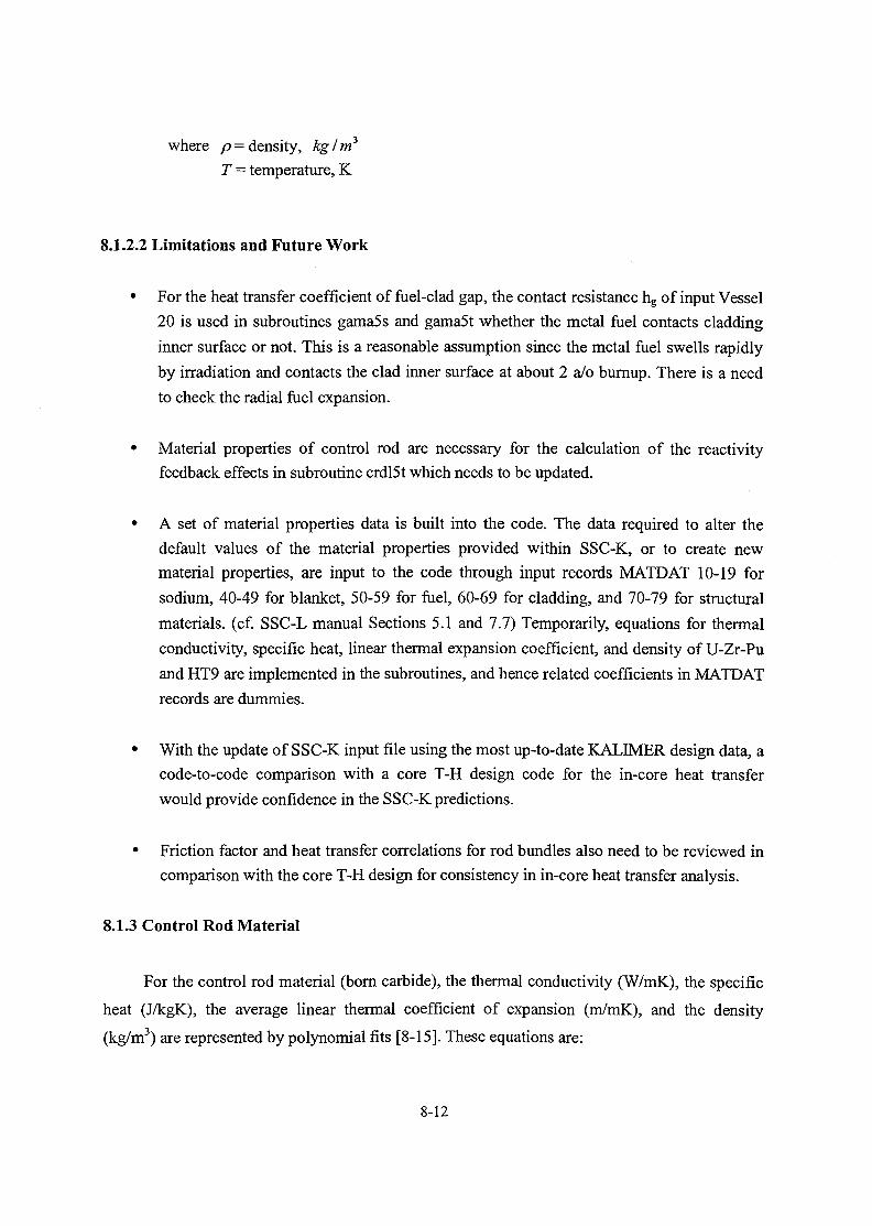
where p= density, kg/m3
T = temperature, K
8.1.2.2 Limitations and Future Work
• For the heat transfer coefficient of fuel-clad gap, the contact resistance hg of input Vessel
20 is used in subroutines gama5s and gama5t whether the metal fuel contacts cladding
inner surface or not. This is a reasonable assumption since the metal fuel swells rapidly
by irradiation and contacts the clad inner surface at about 2 a/o bumup. There is a need
to check the radial fuel expansion.
• Material properties of control rod are necessary for the calculation of the reactivityfeedback effects in subroutine crdl5t which needs to be updated.
• A set of material properties data is built into the code. The data required to alter the
default values of the material properties provided within SSC-K, or to create new
material properties, are input to the code through input records MATDAT 10-19 for
sodium, 40-49 for blanket, 50-59 for fuel, 60-69 for cladding, and 70-79 for structural
materials, (cf. SSC-L manual Sections 5.1 and 7.7) Temporarily, equations for thermal
conductivity, specific heat, linear thermal expansion coefficient, and density of U-Zr-Pu
and HT9 are implemented in the subroutines, and hence related coefficients in MATDAT
records are dummies.
• With the update of SSC-K input file using the most up-to-date KALIMER design data, a
code-to-code comparison with a core T-H design code for the in-core heat transfer
would provide confidence in the SSC-K predictions.
• Friction factor and heat transfer correlations for rod bundles also need to be reviewed in
comparison with the core T-H design for consistency in in-core heat transfer analysis.
8.1.3 Control Rod Material
For the control rod material (born carbide), the thermal conductivity (W/mK), the specific
heat (J/kgK), the average linear thermal coefficient of expansion (m/mK), and the density
(kg/m3) are represented by polynomial fits [8-15]. These equations are:
8-12

\kx+k2T
(8-39)
(8-40)
and
[n-«(r)(r-r0)](8-41)
These equations are similar in form to Equations (8-1), (8-2), (8-7) and (8-12), respectively.
Values for the various parameters are noted in Table 8-4, and P is the porosity, which is an input
quantity read in with the control rod geometric data. These coirelations are valid in the
temperature range from 500 K to 1250 K.
8.1.4 Sodium
All of the required thermo-physical properties for liquid sodium and sodium vapor are
taken from Golden and Tokar [8-16]. These are noted as follows:
Thermal Conductivity (W/mK)
The thermal conductivity of liquid sodium is given by the following equation:
k(T) = ko + k,T + k2T2 (8-42)
where
k0 =109.7 ,
= -6.4499 *10~2
k2 =1.1728*10"-5
8-13

Specific Heat Capacity (J/gK)
The specific heat capacity at constant pressure for liquid sodium is given by
(8-43)
where
c0 =1630.22 ,
c, =-0.83354 ,
c2 =4.62838 * 10"
Table 8-4
Parameters for Control Rod Material Properties
ParameterKoK,K2
K3
K4K5
Coc,c2C3
c4c5c6aoaiPoTo
Value334.1321.61780.053810.02.20.01741.792.34856*10-4
0.00.00.00.0-46,634.7-1.4886*10"3
4.124*10"6
2381.0295.4
Enthalpy (J/kg)
The enthalpy of saturated liquid sodium is given by
(8-44)
8-14
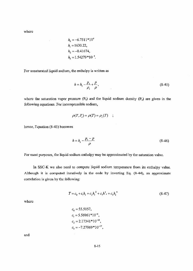
where
ho= -6.7511*104
^=1630.22,
^ = - 0 . 4 1 6 7 4 ,
h, = 1.54279 nO"4.
For unsaturated liquid sodium, the enthalpy is written as
h = hs-^ + £, (8-45)Ps P
where the saturation vapor pressure (Ps) and the liquid sodium density (Ps) are given in the
following equations. For incompressible sodium,
hence, Equation (8-45) becomes
h = h s - ^ ^ - (8-46)P
For most purposes, the liquid sodium enthalpy may be approximated by the saturation value.
In SSC-K we also need to compute liquid sodium temperature from its enthalpy value.
Although it is computed iteratively in the code by inverting Eq. (8-44), an approximate
correlation is given by the following:
where
= co + c,ft, + c2hs2 + c3h\ + c+h* (8-47)
c o= 55.5057,
c,= 5.56961 HO-4,
c2=2.17341*10-10,
c3=-7.27069 *10"17,
and
8-15

c4=4.41118*10-24.
Saturation Vapor Pressure (Pa or N/m2)
The saturation vapor pressure of sodium is expressed by the following two equations:
T for T<TX (8-48)
and
logl0^=P4 + P5/r + P61og10r for T >TX (8-49)
where
Pi= 11.35977 ,
P2=-5567.0 ,
P3=-0.5 ,
P4= 11.68672 ,
P5= -5544.97 ,
P6=-0.61344 ,
and
Ti= 1144.2.
The saturation temperature of liquid sodium as a function of pressure is given by the following
equation [8-17]:
Ts = —. C° t . (8-50)In (9.869 *10-6P)-c,
where
C0=-1213.0
Ci=10.51
and P is the pressure in N/m2 .
Density (kg/m3)
The density of saturated liquid sodium is given by the following relation:
for TX<T<T2 (8-51)
where,
8-16

p0 =1011.597
p, =-0.22051,
/72=-1.92243*10~5,
p3= 5.63769 *10"9,
Tx =370.9,
and,
r2 =1644.2 .
The density of unsaturated liquid sodium is related to that of saturated liquid through a
compressibility factor (PT), as follows:
p(T, P) = ps(T) exp [pT {p - ps)\ (8-52)
where ps(T) is given by Equation (8-51) and Ps is given by Equations (8-48) or (8-49). If
incompressibility is assumed, PT =0. Hence,
(8-53)
Dynamic Viscosity ( PI, i.e. ,N s/m2)
The dynamic viscosity of liquid sodium is represented as
| r (8-54)
where
C,=-2.4892,
C2=220.65 ,
and
C3=-0.4925 .
Heat of Vaporization (J/kg)
The heat of vaporization, fitted over the range 1150 to 1500 K is given by the following equation
[8-17]:
8-17

(8-55)
where
^ = 4.40241 *106,
4 =-17.5055,
^=-0.380184.
Specific Heat Capacity (J/kg K)
The specific heat capacity at constant pressure for sodium vapor was fitted over the range 1150
to 1500 K, and is given by the equation [8-17]:
2 (8-56)
where
c0=4.4015*103,
c, = -2.2987,
c2= 6.347 *10'4.
Density (kg/m3)
The density of sodium vapor is given by the following equation:
(S-57)
in which the factor A(T) was fitted over the range 1150 to 1600 K and is given by the equation
[8-17]:
2 (8-58)
where
8-18

a0=3.27317*10"3,
a, = -8.72393 *10~7,
a, = 6.07353 *10-10.
Enthalpy (J/kg)
At a given reference pressure p, the sodium saturation temperature Ts is first calculated. The
liquid saturation enthalpy hi(Ts) and heat of vaporization X (Ts) are then calculated. The vapor
enthalpy is then given by the equation
{J-Tsf^hv,iJ-Tsf (8-59)
where
/?n=4.4015*103,
hV2 =-1.14935,
/V3=2.11567*1CT\
X (Ts) is given by Eq.(8-55), and hi(Ts) is given by Eq.(8-44).
8.1.5 Water and Steam
The constitutive relations for water are currently given by correlations where the properties
are evaluated as a function of enthalpy (H) and pressure (P) [8-18].
Enthalpy of Saturated Liquid (J/kg)
The enthalpy of saturated water is given by
Hi (p) = «o + a\P + aiP2 +a3p3+ a4p
4 + a5p5 (8-60)
where
8-19
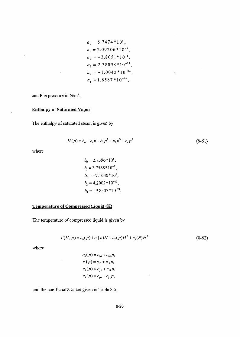
a0 = 5.7474*105,
a, -2.09206*10-',
a2 = -2.8051*10'
a, = 2.38098*10
a4 =-1.0042*10
a5 =1 .6587*10
and P is pressure in N/m2.
Enthalpy of Saturated Vapor
The enthalpy of saturated steam is given by
-15
-22
- 3 0
+ b4p4 (8-61)
where
Z?0=2.7396*106,
-2Z>,=3.7588*10,
Z>2=-7.1640*109,
^=4.2002*10-,-16
b4 =-9.8507*10,-24
Temperature of Compressed Liquid (K)
The temperature of compressed liquid is given by
T(H,p) = co(p) + c1(p)H + c2(p)H2 +c3(P)H3 (8-62)
where
and the coefficients cy are given in Table 8-5.
8-20

Temperature of Superheated Vapor (K)
The temperature of superheated steam is given by
(8-63)
where
and the coefficients dy are given in Table 8-6.
Density of Compressed Liquid (kg/m3)
The density of compressed water is given by
,p) = f1+f2H2+f3H\ for #<6.513*10 5J/% (8-64)
, for H>6.5\3*105J/kg (8-65)
The coefficients § are given in Table 8-7.
8-21

Table 8-5
Values of Coefficients for Temperature of Compressed Liquid Water
CoefficientCooCoiCioC n
C20C21C30C31
Value2.7291*102
-1.5954*10"7
2.3949*10'4
-5.1963*10"°5.9660* 10'12
1.2064*10"18
-1.3147*10"17
-5.6026*10"25
Table 8-6
Values of Coefficients for Temperature of Compressed Water Vapor
Coefficient
doodiod20doidnd2ido2d32
d22
Value6.5659*10^-S.256^10-4
1.6221*10"10
9.9066* 10"5
-3.4406* 10"n
1.8674*10"18
-2.1879*10"12
7.0081 *10"19
-1.4567*10"26
Table 8-7
Values of Coefficients for Density of Compressed Liquid Water
Coefficientfif2f3Ufsf6
Value999.65+4.9737*10";*p
-2.5847*10-10+6.1767*10"19*p1.2696* 10"22-4.9223* 10"3' *p
1488.64+1.3389*10"6*p1.4695*109+8.85736*p
3.20372*106+1.20483*10"2*p
8-22
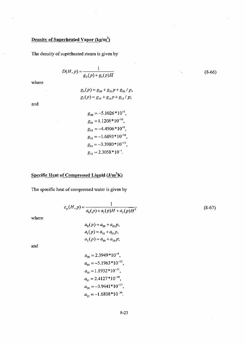
Density of Superheated Vapor (kg/m )
The density of superheated steam is given by
(8-66)go(P) + gi(P)H
where
and
g o o = -5.1026*10-s,
g01-1.1208*10-10,
gO2=-4.4506*10+5,
glo = -1.6893*l(r10,
gn=-3.3980*10-17,
^,2=2.3058*10"'.
Specific Heat of Compressed Liquid (J/m3K)
The specific heat of compressed water is given by
cp (H> P) =
where
and
000= 2.3949 *10"4,
aO]=-5.1963*10~13,
0,0=1.1932*10"",
-17
' 2 4
a20= -3.9441*10
a21=-1.6808*10'24.
8-23

Specific Heat of Superheated Vapor (J/m3K)
The specific heat of superheated steam is given by
cp (H, p) = (8-68)bQ(p) + bx(P)H
where
and
6oo = -5.2569 *1(T\
^,=-3.4406*10"",
bO2= 7.0081 *1(T19,
&10=3.2441*10-10,
6n=3.7348*10"18,
612=-2.9134*10-26.
Viscosity of Compressed Liquid (Ns/m2)
The viscosity of compressed water is given by
eo{H) = 6^ + e01H + e02H2 + e03H
3
n(H,p) = co + c,x + c2x2 + c3x
3 + c4x4 -[do + dlE + d2E
2 + d3E2)(p-pl) H<Hi (8-69)
n(H, p) = e0 (H) + ex (H)(p -Pl) H,<H<H2 (8-70)
n(H,p) = fo+f1z + f2z2+f,z3 + f4z
4 H>H2 (8-71)
where
X = go(H-gl),
8-24

and the coefficients are given in Table 8-8.
Table 8-8
Values of Coefficients for Viscosity of Compressed Liquid Water
Coefficient
CoCi
c2c3c4dodid2
d3
eooeOieo2eO3eioenenfl3fofl
f2f3U
HiH2
Pigogig2g3g4g5
Value1.2995*10°
-9.2640* 10"4
?>.%\Q5*\<y*-8.2164*10"5
7.0224* 10"6
-6.5959* 10-12
6.763*10"12
-2.8883*10'12
4.4525* 10-13
1.4526*10-3
-6.9881 *10"9
1.5210*10-14
-1.2303*10'20
-3.8064* 10'11
3.9285*10-16
-1.2586*10-21
1.2860*10-27
3.0260* 10-4
7.5671*10'5
-1.6479*10-5
1.4165*10-6
2.76* 105
3.94*105
6.8946* 105
8.5813*10"6
4.2659* 104
6.4845* 10-6
5.5359*104
3.8921*10"6
4.0147*105
8-25

Viscosity of Superheated Vapor (Ns/m )
The viscosity of superheated steam is given by
for r<300.K: (8-72)
for 300<T<315K (8-73)
n(H,p) = for T>375K (8-74)
where
T = Tv(H,p) -273.15,
D = Dv(H,p),
and the coefficients are given in Table 8-9.
Table 8-9
Values of Coefficients for Viscosity of Superheated Water Vapor
Coefficientaoaibob j
CoCi
c2c3dodid2
d3
eo
e2
Value4.07* 10"°8.04* 10"6
1.858*!©"1
5.9* 10"10
-2.885* 10"6
2.427* 10"8
-6.7893*10""6.3170*10"14
1.76*102
-1.64.8* 10'3
-4.7407* 10'6
3.53*1O"8
1.021*10"14
8-26
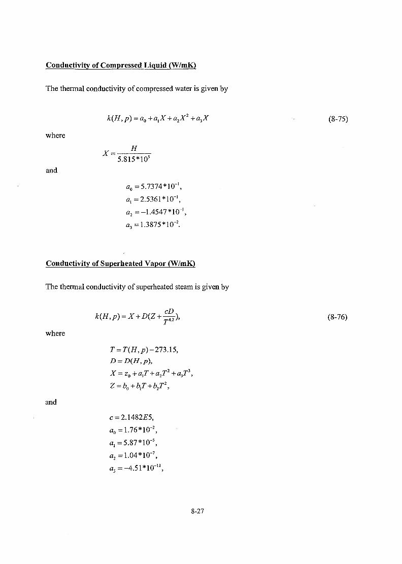
Conductivitv of Compressed Liquid (W/mK)
The thermal conductivity of compressed water is given by
2+a3X (8-75)
where
x = H
5.815*105
and
ao= 5.7374* 10"1,
a1=2.5361*10"1,
a2 =-1.4547*10"',
a3=1.3875*l(T2.
Conductivity of Superheated Vapor (W/mK)
The thermal conductivity of superheated steam is given by
cD^I), (8-76)
where
T = T(H,p)-273.l5,D = D{H,p),
and
c = 2.1482£5,
a0=1.76*10"2,
a,=5.87*10"5,
a2=1.04*10"7,
a3=-4.51*10-n,
8-27

60=1.0351*10-\
£,=4.198*10-7,
b,= -2.771 *10-u.
In addition to the properties listed above, various partial derivatives of many of the functions
were required. These are obtained by analytically differentiating the appropriate correlations.
8.2 Correlations
The required pressure drop and heat transfer correlations for the range of interest are
included in this section. Representative valves for various curve-fitted parameters are noted in SI
units.
8.2.1 Friction Factor Correlations
8.2.1.1 Pressure Drop in Pipe
In the SSC-K code, the Darcy-Weisbach friction factor,^ is computed from correlations
for laminar and turbulent flows with interpolation in the transition regime. There are two
turbulent flow fiction factor models. The first model computes the turbulent friction factor using
an engineering approximation to the well-known Colebrook-White correlation, while the second
model uses an exponential friction with user's input coefficients. The frictional pressure drop in
the different subchannels of core is calculated by specifying different friction factors. However
the default friction law which applies globally throughout the system is specified in the function
of FRIC in the SSC-K code.
The friction pressure drop across a pipe of length L, when the developing flow region can
be ignored, is given by
_ . „ . _=r_, p _p =fLpUlXrfriction ~ I , 1 in 1 outfiicth" K [ dz 1 in ""' D 2
- v azj uu z ( 8 7 y )
where Dh is the hydraulic or equivalent diameter in the case on non-circular channels, defined as
8-28
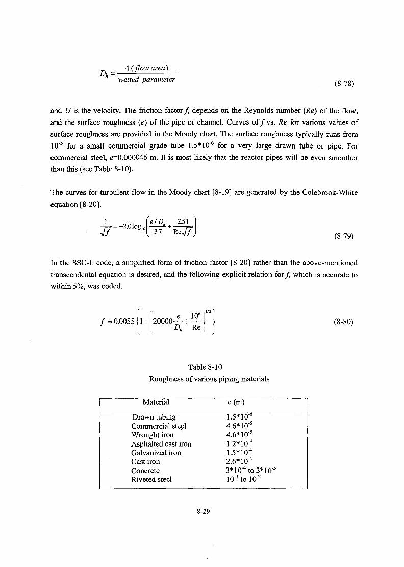
A,=4 {flow area)
wetted parameter (8-78)
and C/ is the velocity. The friction factor/ depends on the Reynolds number (Re) of the flow,
and the surface roughness (e) of the pipe or channel. Curves of /vs . Re for various values of
surface roughness are provided in the Moody chart. The surface roughness typically runs from
10 for a small commercial grade tube 1.5*10 for a very large drawn tube or pipe. For
commercial steel, e=0.000046 m. It is most likely that the reactor pipes will be even smoother
than this (see Table 8-10).
The curves for turbulent flow in the Moody chart [8-19] are generated by the Colebrook-White
equation [8-20].
(8-79)
In the SSC-L code, a simplified form of friction factor [8-20] rather than the above-mentioned
transcendental equation is desired, and the following explicit relation for/ which is accurate to
within 5%, was coded.
/ = 0.0055 U + 20000—1/3 1
^ 1Dh ReJ
(8-80)
Table 8-10
Roughness of various piping materials
Material
Drawn tubingCommercial steelWrought ironAsphalted cast ironGalvanized ironCast ironConcreteRiveted steel
e(m)
1.5*10"4.6* 10-5
4.6*10"5
1.2*10"4
1.5*10"4
2.6* 10"4
3*10"4to3*Kr3
10-3tol0"2
8-29
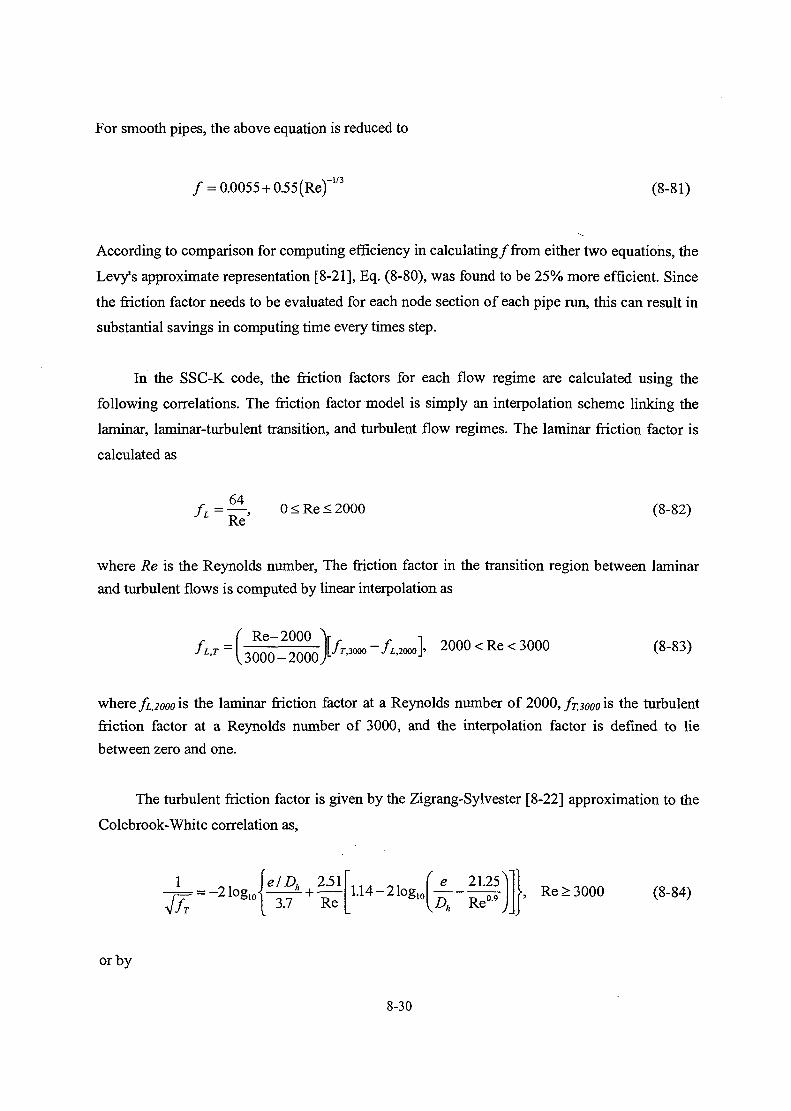
For smooth pipes, the above equation is reduced to
/ = 0.0055 + 0.55(Re)~1/3 (8-81)
According to comparison for computing efficiency in calculating/from either two equations, the
Levy's approximate representation [8-21], Eq. (8-80), was found to be 25% more efficient. Since
the friction factor needs to be evaluated for each node section of each pipe run, this can result in
substantial savings in computing time every times step.
In the SSC-K code, the friction factors for each flow regime are calculated using the
following correlations. The friction factor model is simply an interpolation scheme linking the
laminar, laminar-turbulent transition, and turbulent flow regimes. The laminar friction factor is
calculated as
/ , = — , 0<Re<2000 (8-82)Re
where Re is the Reynolds number, The friction factor in the transition region between laminar
and turbulent flows is computed by linear interpolation as
fLT=\ R e ~ 2 0 Q 0 \fTVna-fL2Oal 2000<Re<3000 (8-83)'T 1,3000-2000/ ' JL,IOOO\> \ )
where fuooo is the laminar friction factor at a Reynolds number of 2000, frjooo is the turbulent
friction factor at a Reynolds number of 3000, and the interpolation factor is defined to lie
between zero and one.
The turbulent friction factor is given by the Zigrang-Sylvester [8-22] approximation to the
Colebrook-White correlation as,
21og\elDh 251
10 1 i n + r>_J [ 3.7 Re
or by
e 21.25>, Re > 3000 (8-84)
8-30

(8-85)
where e is the surface roughness, A, B, and C are user input constants, and the other variables
have been defined previously. The Zigrang-Sylvester equation has the advantage that it is an
explicit relation for the friction factor, while the Colebrook-White correlation is a transcendental
function requiring iteration for the determination of the friction factor. The Zigrang-Sylvester
approximation to the Colebrook-White correlation for turbulent flow., has a mean square error of
0.1% and a maximum deviation of 0.5% when compared to the Colebrook-White correlation
over the ranges 0.5 > e/Dh > 10"5 and 107 > Re > 2500.
It should be noted that the Moody charts are generated based on isothermal fluid flow. In
the presence of heat transfer at the wall, either the fluid properties, such as viscosity and density
should be evaluated at a film temperature. The film temperature is assumed to be average of wall
temperature (Tw) and bulk temperature of coolant (Tb). The computed value for / should be
modified as follows.
(8-86)
where n is constant. Generally, for steady-state flow in a pipe,/mOdified=/ These two values are
different under transient condition, however, the difference is considered small enough to be
neglected.
Pressure losses due to fittings, valves, bends, contractions, and expansions are computed
from
1 (8-87)
where C/is the average velocity in the smaller cross section if there is a change in cross section in
the fitting involved. These objects cause the flowing fluid to lose energy owing to a sudden
change of cross section or change of direction. Such a loss in energy proportional to square of
velocity, and unlike wall friction, has little if any dependence upon Reynolds number and
relative roughness. In general, the effects of fittings and valves are evaluated by the velocity-
head-loss coefficient K. These data can be obtained from typical pipe; fittings and other changes
8-31

as shown in Table 8-11 [8-23].
Table 8-11
Form Loss Coefficient for Various Flow Restrictions
Parameter
Pipe entrance from a plenumWell rounded entrance to pipeSlightly rounded entrance to pipeSharp-edged entranceProjecting pipe entrancePipe exit to plenumAny pipe exitSudden changes in cross-sectional area
Sudden contractionSudden expansionwhere /? = small cross-sectional area
large cross-sectional area
Fittings (Z/D)equiv90° Standard elbow 3090° Large-radius elbow 2045° Standard elbow 16Standard tree 20(flow through run)
Standard tree 60(flow through branch)
Valves (various types)Fully openHalf-closed
K
0.040.230.500.78
1.0
0.5(1- P2)I-/?2
0.35-0.90.2-0.60.17-0.450.2-0.6
0.65-1.7
0.15-15.0
Reference velocity
In pipeIn pipeIn pipeIn pipe
In pipe
DownstreamUpstream
8-32

8.2.1.2 Pressure Drop in Wire-Wrapped Rod Bundles
Methods of calculating pressure drop in core assemblies In LMFBR are similar to
conventional approaches. The pressure drop across a core assembly consists of (i) entrance and
exit pressure losses between the vessel plena and the core internals, (ii) the friction pressure drop
along the fuel rods, and (iii) the form losses due to the presence of spacers. The entrance and exit
losses are those due to a sudden change in flow area, loss through assembly inlet nozzle, rod
bundle, assembly outlet, etc. Generally, empirically determined pressure-loss correlations have
been used for wire-wrapped rod bundle applications. Attention hen; is focused on the friction
along the wire-wrapped rod bundles.
(1) Engel, Markley, and Bishop
Based on limited experimental data, Engel, Markley, and Bishop [8-24] have
recommended the following generalized correlation for hexagonal fuel assembly applicable in
the range P/D < 1.23 and H < 30 cm.
whereX = 0.0, for Re < 400,
Re-400 400 < Re < 5000
4600
Z = l-0, for Re >5000
and the coefficient A is a function of wire-wrap lead H and pitch to rod diameter ratio.
(8-89)
Note that the wire-wrap lead H in above equation is in centimeters.
(2) Chan and Todreas
8-33
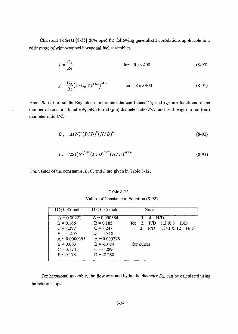
Chan and Todreas [8-25] developed the following generalized correlations applicable to a
wide range of wire-wrapped hexagonal fuel assemblies.
1 for Re < 400 (8-90)
for Re > 400 (8-91)
Here, Re is the bundle Reynolds number and the coefficient Cis and Cje, are functions of the
number of rods in a bundle N, pitch to rod (pin) diameter ratio P/D, and lead length to rod (pin)
diameter ratio H/D.
= A{N)\PID)c(HID)1(8-92)
Ci9=25l{Nfm'{P/Df99l{H/D) (8-93)
The values of the constant A, B, C, and E are given in Table 8-12.
Table 8-12
Values of Constants in Equation (8-92)
D > 0.35 inch
A = 0.00221B = 0.166C = 8.297E = -1.457A = 0.0000395B = 0.063C = 0.174E = 0.178
D < 0.35 inch
A = 0.000584B = 0.185C = 8.247D = -1.818A = 0.000278B = -0.084C = 0.289D = -0.268
]
1.for 2.
3.
Vote
4P/DP/D
for others
H/D1.2 & 8 H/D1.343 & 12 H/D
For hexagonal assembly, the flow area and hydraulic diameter Dh, can be calculated using
the relationships:
8-34

(8-94)
Perimeter = (2&df_f ) + nN(D + Dw) (8-95)
Here, d/.f is the distance between the flat surfaces of hexagonal assembly, D is the pin diameter,
Dw is wire-wrap diameter, and n is the number of pins in a bundle.
(3) Experiments for fuel assemblies of CRBR and FFTF
In the Clinch River Breeder Reactor (CRBR) plant, there are several different types of
hexagonal rod bundles. The important geometrical characteristics of these bundles are presented
in Table 8-13. Based on the experimental measurements [8-26-29], several different correlations
for friction factor are recommended for CRBR and Fast Flux Test facility (FFTF) fuel
assemblies. The same correlations are applicable to both FFTF and CRBR fuel assemblies. Three
sets of correlations for friction factors of in-core assemblies are availalble in the SSC-K code.
Table 8-13
Important Parameters of CRBR Hexagonal Assemblies
Assembly No. of pins P/D H/D D(mm)
FuelBlanketPrimary controlSecondary controlReactor shield
21761373119
Dh(mm)
1.241.0721.051.051.0
51.747.90521.1810.87
-
5.84212.85215.29114.03625.197
3.2543.3996.86215.9811.357
Fuel Assemblies (L6ATYP* 2 or 3)
f = Min\--, for Re < 800 (8-96)
(8-97)
8-35

Blanket Assemblies (L6ATYP= 2)
= Min< ,0.5 for Re < 400 (8-98)
110 Re-400 0.48 Re-400+Re 4600 4600
for 400SRe<5000 (8-99)
0.48
Re025f o r Re > 5000 (8-100)
Control Assemblies
f = Min\ — ,05 \iRe J
(L6ATYP= 3)
for Re < 800 (8-101)
/ = — + (0.316Re-025 - 84Re) Re~ 8 ° ° j
Re v ; 1200for 800 < Re < 2000 (8-102)
N 0.885
for Re>2000 (8-103)
Here, P/D is assembly pitch to diameter ratio and (P/D)w is wire wrap pitch to diameter ratio.
Constants A and B are supplied by user as input.
For the inlet orifice region and bypass region, SSC-K uses the following corrections.
Min\ — ,05 for Re < 2000 (8-104)
= 0.316Re"025 for Re > 2000 (8-105)
8-36

8.2.2 Heat Transfer Correlations
Heat transfer correlations for liquid metal turbulent flow in channels or rod bundles are in
the form of:
B(Pef (8-106)
where the Peclet number Pe, is the product of the Reynolds and Prandtl numbers. A, B, and C are
constants that depend on the geometry and the boundary conditions. The constant C is a number
close to 0.8. The constant A reflects the fact that significant transfer in liquid metals occurs even
as Re goes to zero.
(1) Circular tube
The following relations hold for the boundary conditions cited and fully developed flow
conditions.
Lyon's correlation for constant heat flux along and around the tube [8-30]
Nu = l + 0.025 Pe08 (8-107)
Seban and Shimazaki's correlation for uniform axial wall temperature and uniform radial heat
flux [8-31]
Nu = 5.0 + 0.025Pe0S (8-108)
Aoki's correlation [8-32]
/— -.0.8
Nu = 6.0+O.O25[0Pe) (8-109)
where
_ 0.014[l — exp(—71.8 )1<l> = (8-110)
X
8-37
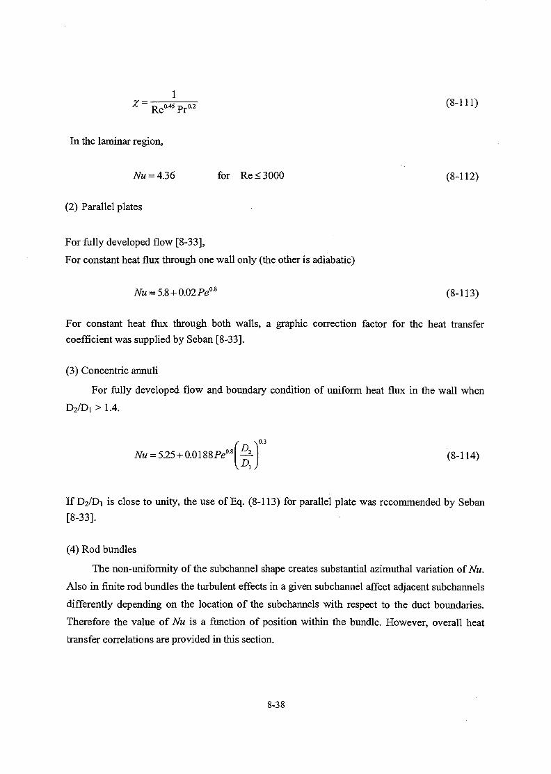
In the laminar region,
Nu = 4.36 for Re <3000 (8-112)
(2) Parallel plates
For fully developed flow [8-33],
For constant heat flux through one wall only (the other is adiabatic)
iVK = 5.8 + 0.02Pe0-8 (8-113)
For constant heat flux through both walls, a graphic correction factor for the heat transfer
coefficient was supplied by Seban [8-33].
(3) Concentric annuli
For fully developed flow and boundary condition of uniform heat flux in the wall when
D2/Di >1.4.
[\0.3
— (8-114)
If D2/D1 is close to unity, the use of Eq. (8-113) for parallel plate was recommended by Seban
[8-33].
(4) Rod bundles
The non-uniformity of the subchannel shape creates substantial azimuthal variation of Nu.
Also in finite rod bundles the turbulent effects in a given subchannel affect adjacent subchannels
differently depending on the location of the subchannels with respect to the duct boundaries.
Therefore the value of Nu is a function of position within the bundle. However, overall heat
transfer correlations are provided in this section.
8-38
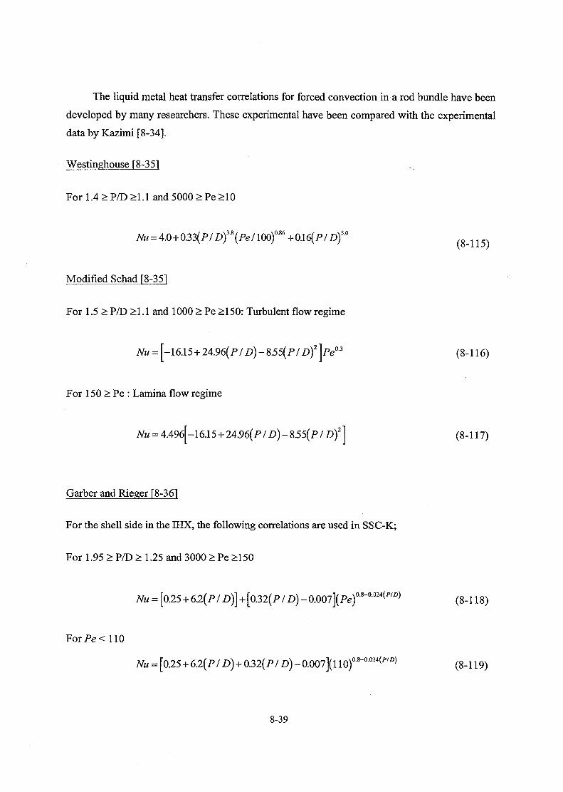
The liquid metal heat transfer correlations for forced convection in a rod bundle have been
developed by many researchers. These experimental have been compared with the experimental
data by Kazimi [8-341.
Westinghouse [8-351
For l .4>P/D>l . l and 5000 >Pe>10
7VM = 4.0+0.33(P/D)3-8(Pe/100)086+0.16(P/Z))50
Modified Schad [8-351
For 1.5 > P/D >1.1 and 1000 > Pe >150: Turbulent flow regime
M* = [-16.15 + 24.96(P/JD)-8.55(P/i))2]Pe0-3 (8-116)
For 150 > Pe : Lamina flow regime
ATM = 4.496[-16.15 + 24.96(P/i))-8i5(P/Z))2] (8-117)
Garber and Rieger [8-361
For the shell side in the IHX, the following correlations are used in SSC-K;
For 1.95 > P/D > 1.25 and 3000 > Pe >150
5l\P ID)- 0.007 \{Pe) (8-118)
ForPe<110
0.007](llO)a8~°0!4(WD) (8-119)
8-39

Borishcnskii et al. F8-371
For 1.5 > P/D > 1.1 and 2000 > Pe >200
12.76(i>/Z>)-3.65(i>/D)2]
+ 0.0174[l - exp 6(1 -PI D)\Pe - 200]09
For 1.5 > P/D > 1.1 and200>Pe
Nu = 24.15 log[-8.12 + 12.76(P / D) - 3.65(P / D)2 ]
(8-120)
(8-121)
Currently In the SSC-K code, Aoki's correlation is used for liquid metal flow in a pipe,
Graber-Rieger correlation for the shell side in the intermediate heat exchanger (IHX), and
Modified- Schad correlation for Rod bundles. Table 8-14 summarizes the correlations used for
both SSC-L and SSC-K.
Table 8-14
Comparison of correlations used for SSC-L and SSC-K
FrictionFactor
HeatTransferCoeffi.
SSC-L
For pipeo Moody Chart, Levy model
For in-core assemblyo CRBR specific experiments for
Fuel, Blanket and Controlassemblies
For circular tubeo Theoretical Nu for laminar flowo Aoki for turbulent flow
For IHX shell-sideo Graber and Rieger
For rod bundleo Modified Schad for both laminar
and turbulent flows
SSC-K
For pipeo Zigrang-Sylvester approximation
For in-core assemblyo Engel, Markley, and Bishopo Chan and Todeaso Generalized FFTF experiments
For circular tubeo Theoretical Nu for laminar flowo Aoki for turbulent flowo Lyon for const, heat fluxo Seban and Shimazaki for const.
temperatureFor IHX shell-side
o Graber and RiegerFor rod bundle
o Westinghouseo Kazimi and Carellio Borishanskii
8-40

The heat transfer correlations for water/steam are given for four different modes of heat
transfer. The first mode of heat transfer is forced convection. The Nusselt number for nucleate
boiling is given as [8-38]:
0.8 T»-.0.4Nu = 0.023 Reu-8Pr
The heat transfer for nucleate boilmg is given as [8-39]:
where the nucleate boiling coefficient IINB is given as:
(8-122)
(8-123)
where
hNB= 0.00122 <v 0.79^,0.45 0.49
K' L> Pi (8-124)
Q = specific heat of liquid
Ki = thermal conductivity of liquid
Q. — surface tension
A.fg = latent heat of vaporization, and
AP = difference in saturation pressure corresponding to the wall superheat.
The Reynolds number correction factor F, and the nucleate boiling suppression factor S arerepresented as:
IF* —
2.84 JL045 A
2.57 + 0.7643—, — >2.(8-125)
1.05-1.3*10^ Re,
0.83-4.3*10"6Re,
0.32exp(-1.92*10~6Re),
0.09
Re<2.5*104
2.5*104<Re<1051
105<Re<6*105
Re>6*105
(8-126)
8-41

and
Re=Re] F 1 2 5
Where Xtt is the Lockhart/Martinelli [8-40] parameter:
o / \0.5 / \0.10
. A if) ( 8 . 1 2 7 )
The convection coefficient he is calculated from the Dittus Boelter equation based on liquid
thermodynamic properties [8-38].
The heat transfer for film boiling regime is given as [8-41]:
0-8Nu = 0.0193Re,0-8 pr ;L23(^.)0-68( £Lf<*\ ( 8 _ 1 2 8 )
Pz Ps
where subscripts 1 and g denote, respectively, liquid and vapor phase at saturation and subscript B
indicates a bulk property of the steam/water mixture.
For superheat steam, the following heat transfer correlation for forced convection is used [8-42]:
Nu = 0.0133Re0-84 Pr0333. (8-129)
The steam/water quality at the DNB point is given by [8-43]:
XBNB= 4-3 8*1 Q 4 / ? ' for <7>6.3*105, (8-130)
HhpgjGI 1350.0 K }
or
4.38 * 104o, .(5.3 *\05/q)1'5
XDNB= 7 ; for 9 <6.3*10 5 (8-131)Dm HpslG/1350.0 H y }
where H]g is the latent heat of vaporization (J/kg), G is the mass flow rate per unit area (kg/s m2),
and q is in W/m2'.
8-42
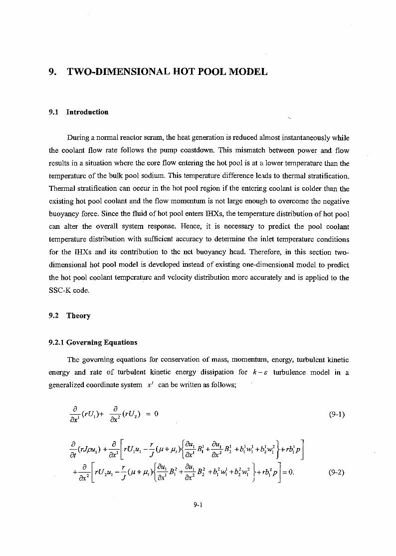
9. TWO-DIMENSIONAL HOT POOL MODEL
9.1 Introduction
During a normal reactor scram, the heat generation is reduced ailmost instantaneously while
the coolant flow rate follows the pump coastdown. This mismatch between power and flow
results in a situation where the core flow entering the hot pool is at a lower temperature than the
temperature of the bulk pool sodium. This temperature difference leads to thermal stratification.
Thermal stratification can occur in the hot pool region if the entering coolant is colder than the
existing hot pool coolant and the flow momentum is not large enough to overcome the negative
buoyancy force. Since the fluid of hot pool enters IHXs, the temperature distribution of hot pool
can alter the overall system response. Hence, it is necessary to predict the pool coolant
temperature distribution with sufficient accuracy to determine the inlet temperature conditions
for the IHXs and its contribution to the net buoyancy head. Therefore, in this section two-
dimensional hot pool model is developed instead of existing one-dimensional model to predict
the hot pool coolant temperature and velocity distribution more accurately and is applied to the
SSC-K code.
9.2 Theory
9.2.1 Governing Equations
The governing equations for conservation of mass, momentum, energy, turbulent kinetic
energy and rate of turbulent kinetic energy dissipation for k-s turbulence model in a
generalized coordinate system x' can be written as follows;
_d_
dx2 = o (9-1)
—(rJpuy) +—jot oxot
dx2
jox
rUxux -
= 0. (9-2)
9-1

9/
J R Pr \dxl ' etc
dx2
Ux L
dx2
*
= o.
J 1 ax2 = rJ{G-pe)
ox
d
dx2
J
1J
1 ac2
where
and
£
(9-3)
(9-4)
(9-5)
£—) (9-6)
(9-7)
(9-8)
9-2
Cex = \M, CS2=1.92, Prt=0.9, C^O.09, ak=l.O, crs=h3 (9-10)
In above equations u{ , T , k , s denote two cylindrical velocity components,
temperature, turbulent kinetic energy and rate of turbulent kinetic energy dissipation respectively.
The geometric coefficients bj represent the cofactors of dy'/dxJ in the Jacobian matrix of the
coordinate transformation, J stands for the determinant of the Jacobian matrix, y' is the
cylindrical coordinate system and p, ju, p, Pr denote densily, viscosity, pressure and
Prandtl number respectively.
9.2.2 Discretization of Governing Equation
The solution domain is divided into a finite number of quadrilateral control volumes and
the discretization of the governing equation is performed following the finite volume approach.
The convection terms are approximated by a higer-order bounded scheme HLPA developed by
Zhu [9-1] and the unsteady terms are treated by the backward differencing scheme.
9.2.3 Momentum Interpolation Method
In the present study, the Rhie and Chow's scheme [9-2] is modified to obtain a converged
solution for unsteady flows which is independent of the size of time step and relaxation factors.
The momentum equations are solved implicitly at the cell-centered locations in the Rhie and
Chow's scheme. The discretized form of momentum equations for the cell-centered velocity
components can be written as follows with the under-relaxation factors expressed explicitly;
9-3

(9-12)
where
UC' AV)}/A;> (9-13)
K -^-v <?-•*>
and au are the under-relaxation factors for u{ velocity components and the superscripts
n — \, / - I denote the previous time step and iteration level, respectively. The discretized form
of momentum equations for the cell-face velocity component, for example M, at the east face,
can be written as follows;
i ).OP, " PE)HD2Ui). (Pse -PJ+ (EUi \tC +d " «„ WC (9-17)
In the present modified Rhie and Chow's scheme, this cell-face (the east face) velocity
component is obtained explicitly through the interpolation of momentum equations for the
neighboring cell-centered cylindrical velocity components. Following assumptions are
introduced to evaluate this cell-face velocity component.
(9-19)
9-4

4^+^JP- (9-20)
where /e+ is the geometric interpolation factor defined in terms of distances between nodal
points. Similar assumptions can be introduced for evaluating the velocity components at the
north face. Using above assumptions, the velocity component uie can be obtained as follows;
At«'-' - f+ v )E u"-x - n - (9-21)
The term in the first bracket of right hand side of Eq. (9-11) is the original Rhie and Chow's
scheme [9-2]. Majumdar [9-3] has revealed that omission of the term in the second bracket leads
to a converged solution that is relaxation factor dependent. Recently., Choi [9-4] added the term
in the last bracket to obtain the converged solution that is independent of the size of time step
and relaxation factors for unsteady flow calculations.
9.2.4 Solution Algorithm
The SIMPLEC algorithm by Van Doormal and Raithby [9-5] is used for pressure-velocity
coupling in the present study. In this algorithm the momentum equations are implicitly solved at
cell-centered locations using Eqs. (9-1) and (9-2). Then the cell-face velocities are evaluated by
Eq. (9-11). Since these starred velocities do not satisfy the continuity equation unless the
pressure field is correct, they should be corrected to satisfy the continuity equation during the
iteration process. The following velocity correction equations are assumed in the SIMPLEC
algorithm.
9-5

(9-22)
(9-23)
Inserting above equations into the continuity equation leads to a pressure correction
equation. After solving the pressure correction equation, the cell-face velocities are corrected by
above equations and the cell-centered velocities are corrected by following equations.
(9-24)
u'2J,=u2J,-u2J,=[ (Dl)P{P:-Pe) + {Dl)p{P:-P'n) ]/[l-ccU2C£A2/Aup>)p] (9-25)
The pressure correction equations as well as other algebraic equations of momentum equations,
energy equation and turbulent transport equations are solved by the strongly implicit procedure
by Stone [9-6] in the present study.
9.2.5 Treatment of Boundary Conditions
At the inlet both the velocity components and turbulent quantities are prescribed. At the
outlet the zero gradient conditions are imposed while the velocity components are adjusted to
satisfy the overall mass conservation. At the symmetry line the symmetry conditions are imposed.
At the wall node both the velocity components are set to zero. For the near-wall control volumes,
the wall shear-stress vector is expressed as a function of the nodal velocity component parallel to
the wall. The wall shear stress is again decomposed in two components along M, and u2,
respectively, to be used as source terms in the corresponding momentum equations. The wall
function method is used for the near-wall nodes.
9-6

9.3 Modeling
As shown in Fig. 9.1, in the case of one-dimensional model the steady-state hot pool
coolant temperature is calculated in MAIN9S using the input values from MAIN9R and the
transient hot pool temperature is calculated in MAIN9T. In UPLS6T the hot pool energy
variation is calculated and is corrected by prediction-correction method in INTG1T. And then
correct hot pool temperature is fixed in UQIV1T. Therefore, two-dimensional hot pool coolant
temperature is calculated by coupling the developed two-dimensional hot pool model with
UPLS6T
As shown in Fig. 9.2, the developed two-dimensional hot pool model consists of three
subprograms, i.e, BFC, FL0W2D and UFL0W2D. In BFC the grid is generated automatically.
In FL0W2D steady-state hot pool coolant temperature and velocity distributions are calculated
and are used as input values of UFL0W2D. In the UFL0W2D coupled with UPLS6T, the
transient hot pool coolant temperature and velocity distributions are calculated. In Figs. 9.3 and
9.4, the flowcharts of each subprogram are illustrated.
The main functions of the subprograms are as follows;
BF grid generation module
BINDEX calculate location adress for the near boundary nodes
BKIND define various boundary conditions
BOUNDP extrapolate pressure at boundary nodes
BOUNDS call appropriate boundary conditions
CDFLUX calculate cross-derivative fluxes
COEFF calculation of algebraic coefficients of transport equations HLPA
scheme on non-uniform grid
COFCON calculate coefficients for pressure correction equation and face
convective fluxes using momentum interpolation (SIMPLEC)
CWCS initializing mass fluxes
FLOSOL solving all the conservation equations transient
GEOMET calculate geometric coefficients and center-points of control volume
INFORM printing important informations
INP read input variables
INPUT read input variables
9-7

MFL0W2D
MUFL0W2D
OUTPUT
PDTST
PROPS
PVFC
SFLOSOL
SOLVE
SOURCE
SSOLVE
SSTART
START
SUSER
TPLOT
USER
numerical solution of incompressible flows on a nonorthogonal grid
using momentum interpolation method - steady
numerical solution of incompressible flows on a nonorthogonal grid
using momentum interpolation method - transient
print output variables
calculate pressure difference
print major output
calculate fluid properties
correct velocity, flux and pressure
solving all the conservation equations - steady
numerical scheme: Stone's strongly implicit method - transient
calculation of sources for the conservation equations
numerical scheme: Stone's strongly implicit method - steady
initialize some variables - steady
initialize some variables - transient
user define module - steady
plotting module
user define module - transient
9.4 Sample Run
9.4.1 Constant Inlet Temperature Increase
The KALIMER design is a pool-type system, with the entirety of the primary heat
transport system contained within the reactor vessel. During normal operation, the sodium core
inlet and outlet temperatures are 386°C and 530 "C, and the other initial conditions used and
important system parameters are listed in Table 9-1. In the case of two-dimensional model, the
hot pool is modeled as shown in Fig. 9.5. The input parameters of the two-dimensional hot pool
model named HP2D are core outlet temperature and flowrate. In the model, the temperature and
velocity distributions in the hot pool are calculated.
Firstly, in the case of constant inlet temperature increase, we compare the prediction
accuracy between one- and two-dimensional hot pool model. During normal operation, the
sodium bulk temperature of the hot pool is 530 °C and flowrate is 2143.1kg/sec. Also the sodium
9-8

velocity distribution in the hot pool is shown in Fig. 9.6. In the case that the hot pool sodium
inlet temperature increases from 530 °C to 647 °C suddenly, the hot pool sodium temperature
increases until it reaches to the inlet temperature. As shown in Fig. 9.7, the temperature
behaviors of the both models are quite different. In the one-dimensional model, the outlet
temperature increases slowly and immediately, and is reached to 645 °C after 420 seconds.
However, in the two-dimensional model, the outlet temperature is not changed until 20 seconds
and then increases steeply. The outlet temperature is reached to 645 °C after 250 seconds.
In two-dimensional model, the outlet sodium temperature is affected by the inlet sodium
temperature change after several tens of seconds during normal operation and is more actual
qualitative prediction than one-dimensional model. The time delay can alter the overall reactor
system response, so that it is necessary to predict the hot pool sodium temperature distribution
with sufficient accuracy.
9.4.2 Unprotected Transient Overpower Events
An unprotected transient overpower (UTOP) event results when positive reactivity is
inadvertently inserted into the core and there is a failure to scram. The limiting case assumption
is that all the control rods are accidently removed. The event is initiated from full power. The
control rods are assumed to begin withdrawing with a speed of 0.67 cents per second. The
control rod stops are set to limit the withdrawal worth to 10 cents. The: UTOP transient results for
hot pool temperatures, power and flow in both cases of one- and two-dimensional models are
shown in Figs. 9-8 through 9-10. As shown in Fig. 9.6, the power reaches a peak of 1.130 and
1.124 times the rated power at 34 and 27 seconds into the transient, and begins to level off at
1.019 and 1.021 times the rated power in the case of one- and two-dimensional model cases,
respectively.
In the case of one-dimensional model, the hot pool inlet temperature increases from a
normal value of 530 °C to a peak of 551 °C and outlet temperature increases from 530 °C to a
peak of 543 °C and then the inlet and outlet temperatures are reestablished at around 542 °C,
which is 12 °C above the initial temperature, as shown in Fig. 9.9. On the other hand, in the case
of two-dimensional model, the hot pool inlet temperature increases from 530 °C to 550 °C and
outlet temperature increases from 530 °C to 546 °C, and then the inlet and outlet temperatures are
9-9

reestablished at around 543 °C, which is 13°C above the initial temperature. The outlet
temperature is not affected by the inlet coolant until 25 seconds.
As a result of this comparison, it is considered that the time delay effect of the hot pool
affects the core inlet sodium temperature. And then core inlet sodium temperature change affects
the reactivity feedback and reactor power also. Therefore, it seems that the two-dimensional
modeling of the hot pool can predict the overall reactor system response more realistic than one-
dimensional model.
9-10
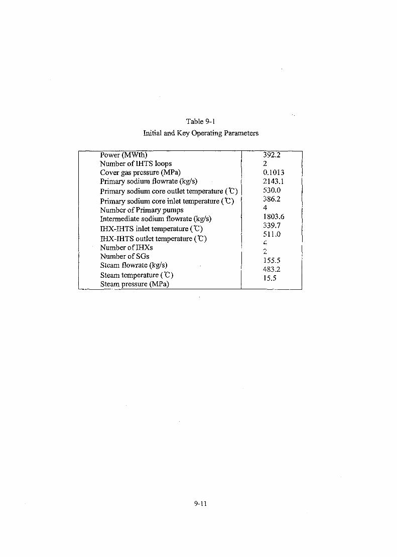
Table 9-1
Initial and Key Operating Parameters
Power (MWth)Number of IHTS loopsCover gas pressure (MPa)Primary sodium flowrate (kg/s)Primary sodium core outlet temperature (°C)Primary sodium core inlet temperature (°C)Number of Primary pumpsIntermediate sodium flowrate (kg/s)IHX-IHTS inlet temperature (°C)IHX-IHTS outlet temperature (°C)Number of IHXsNumber of SGsSteam flowrate (kg/s)Steam temperature (°C)Steam pressure (MPa)
392.220.10132143.1530.0386.241803.6339.7<n 1 AMl.UAHr
1,
1 JJ.J
483.215.5
9-11

START J 1-Dim. Hot Pool Model
MAIN9R
MAIN9S- PBAL9S. Tsan, T'm.. W1U;U. - know 2 of 3 from inputCalculates the unknown variable using known 2 vanables
COOL6S- OPTN6S" UPLN6S: Calculates E^
MAIN9T • INIT9T INIT6T. Calculates initial values of T^u, rMAB>
DRIV9T'
t=t+At
DRIV1T INTG1T: Prediction of the Y1(KK), Y1(KK*1) from old Y1DYDT
JLEQIV1T(2). Reset integrated vanables - TW)U, TUAB
T.V, = Y1(KK). T M =
FLOW1T UPLN6T- UPLS6T: Updates Y1DYDTand calculates T ^
Y1DYDT(KK) = AEA
Y1DYDT(KK+1) = AEE
INTG1T: Correction of the Y1(KK), Y1(KK+1) from new Y1DYDT
EQIV1T(2): Reset integrated variables -
Fig. 9.1 Flowchart of One-dimensional Hot Pool Model
9-12

START J 2-Dim. Hot Pool Model
MAIN9R
INPUT: Hot Pool Geometry
G r i d generation module for the hot pool
Steady-state calculations for the hot pool
Unsteady-state calculations for the hot pool
MAIN9S • PBAL9S: T ^ , T ^ , W.LOIS, - know 2 of 3 from inputCalculates the unknown variable using known 2 variables
COOL6S- OPTN6S- UPLN6S • Calculates ^
C^J-L - E(l uun]
I N P U T : P* H» CPL. K, T« D,, V,
MAIN9T • INIT9T INIT6T - Calculates initial values of T
' IJIIA = ' ( ' -MXIR) '».Aa-
DRIV9T DRIV1T INTG1T: Prediction of the Y1(KK), Y1(KKH) from o/dY1DYDT
EQIV1T(2): Reset integrated variables - except ! „C-f T - T T - T
FLOW1T UPLN6T UPLS6T: Updates Y1DYDT
and call UFLOW2D
'tTHL ~ ''jnruLVi
TINTG1T: Correction of the Y1(KK), Y1(KKH) from newYIDYDT
EQIV1T(2): Reset integrated variables - except ! „ „ ,
Fig. 9.2 Flowchart of Two-dimensional Hot Pool Model
9-13

Fig. 9.3 Flowchart of HP2D; Steady-State
9-14
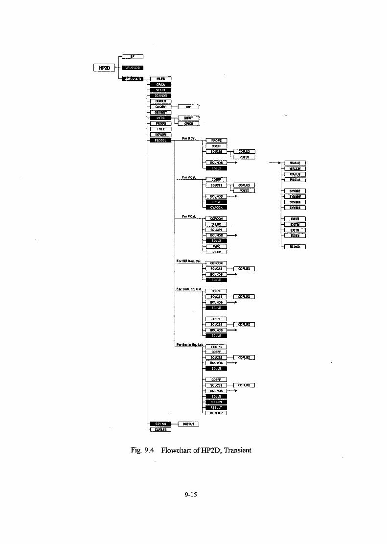
Fig. 9.4 Flowchart of HP2D; Transient
9-15

Axi-symmetry
(U)
1+1
I
J J+1
uoo
-5
INPUT: Pin Cp,n! K, Tw D,n) V,n \'Hf\
t t tt
• 9.5 (I5=97) :free surface
•7.7(I4=79)•7.2(I3=74)- 6.7 (12=69)
CO
o
&to
-0.0 Core Top (l=2)
O C3 —v—».o -~) '-J bot
•3 Ji. "too
Fig. 9.5 Two-Dimensional Hot Pool Model
9-16

MilIII!III!imim
hutI l l lI l l l
Illl
J '" l9/11U
Fig. 9.6 Sodium Velocity Distribution in Hot Pool during Normal Operation
9-17
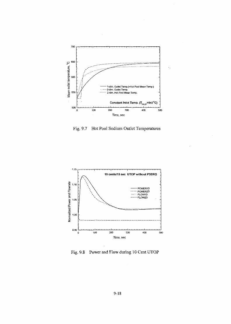
700
500 L - "
- 1-dim. Outlet Temp.(=Hot Pool Mean Temp.)• 2-dim. Outlet Temp.• 2-dim. Hot Pool Mean Temp.
Constant Inlet Temp. (T|NLET=647°C)
100 200 300
Time, sec
400 500
Fig. 9.7 Hot Pool Sodium Outlet Temperatures
1.15
10 cents/15 sec UTOP without PSDRS
P0WER1DP0WER2DFL0W1DFLOW2D
100 200 300 400 500
Fig. 9.8 Power and Flow during 10 Cent UTOP
9-18
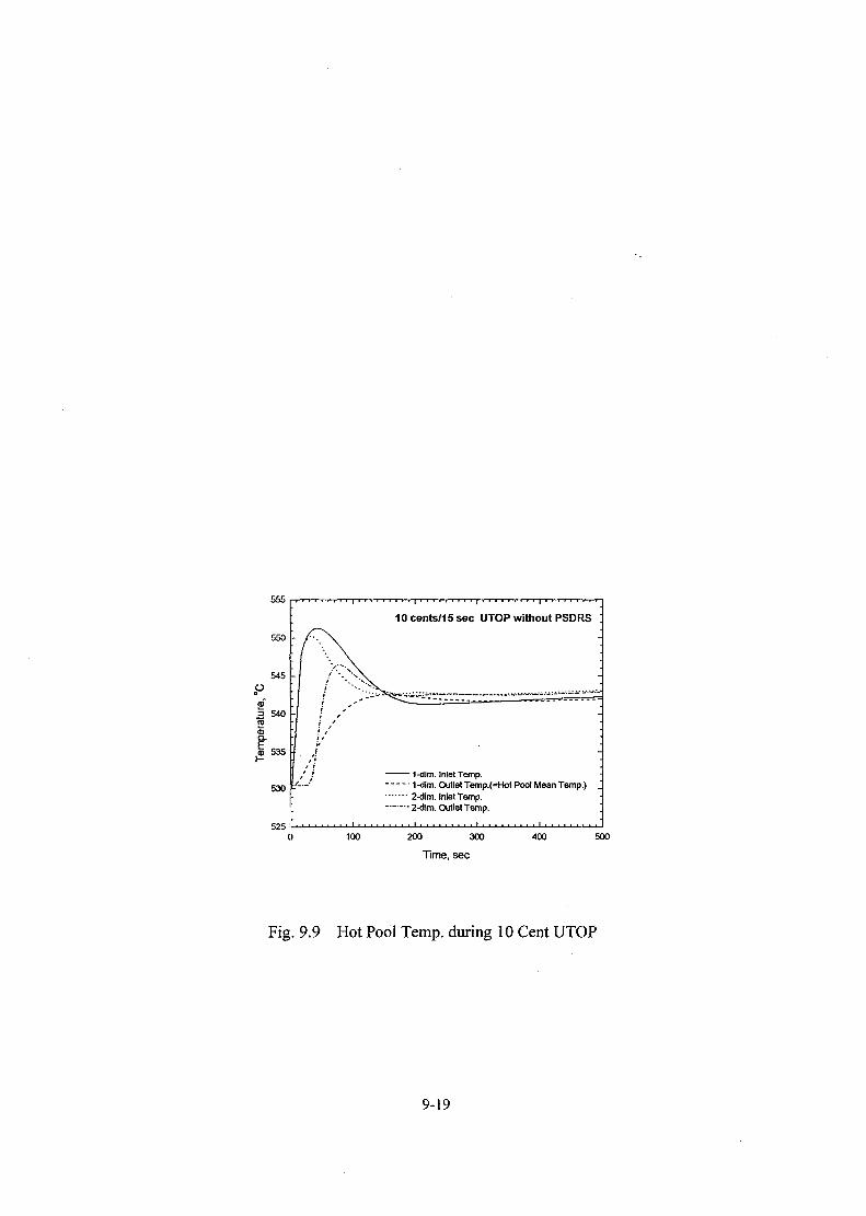
555
525100
10 cents/15 sec UTOP without PSDRS
1-dim. Inlet Temp.1-dim. Outlet Temp.(=Hot Pool Mean Temp.)2-dim. Inlet Temp.2-dim. Outlet Temp.
200 300
Time, sec
400 500
Fig. 9.9 Hot Pool Temp, during 10 Cent UTOP
9-19
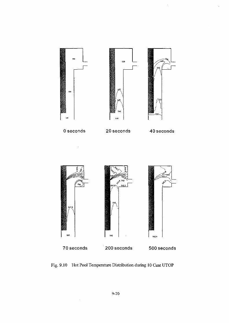
0 seconds 20 seconds 40 seconds
<O
A
70 seconds 200 seconds 500 seconds
Fig. 9.10 Hot Pool Temperature Distribution during 10 Cent UTOP
9-20
REFERENCES
1-1 C. K. Park, et. al. "KALIMER Design Concept", KAERI/TR-88S/97.
1-2 J. G. Guppy, et al., "Super System Code - An Advanced Thermohydraulic Simulation
Code for Transients in LMFBRs," NUREG/CR-3169, BNL, (1933).
6-1 Lee W. Johnson et al, "Numerical Analysis", Addson-Wesley Publishing Company
8-1 LIFE-II Committee, ANL, Priv. Comm, (1973).
8-2 R.G. Gibbym, L. Leibowitz, J.F. Kerrisk and D.G Clifton, "Analytical Expressions for
Enthalpy and Hear Capacity for Uranium-Plutonium Oxide," HEDL-TME 73-60, June
(1973).
8-3 B.F. Rubin, "Summary of (U,Pu) O2 properties and Fabrication Methods, "GEAP-1582,
(November 1970).
8-4 M.F. Lyons, et al., "UO2 Properties Affecting Performance," Nucl. Eng. & Design 21,
167(1972).
8-5 Thermophysical Properties of Matter, "Thermal Radioactive Properties of Non-Metallic
Solids," Vol. 8 edited by Y.S. Touloukian (1972).
8-6 "Mechanical and Physical Properties of the Austenitic Chromium-Nickel Stainless Steels
at Elevated Temperature," The International Nickel Company, Inc., New York (1963).
8-7 C.S. Kim, "Thermophysical Properties of Stainless Steel," ANL 78-55 (1975).
8-8 J. Humphries, "On the Thermal Emittance of Stainless Steels," J. of British Nucl. Energy
Soc. 1,271 (1974).
8-9-8-14 blank
R-l
8-15 "A Compilation of Boron Carbide Design Support Data for LMFBR Control Elements,"
HEDL-TME 78-19 (1975).
8-16 G.H. Golden and J.V. Tokar, "Thermophysical Properties of Sodium," ANL-7323 (August
1967).
8-17 F.E. Dunn, G.J. Fischer, T.J. Heams, P.A. Pizzica, N.A. McNeal, W.R. Bohl and S.M.
Prestein, "The SAS2A LMFBR Accident Analysis computer Code," ANL-813 8
(October 1974).
8-18 W. Wulff, et al., "Development of a Computer Code for Thermal hydraulics of Reactors
(THOR)," Fifth Ouarterly Progress Report, Sect. 3.2, BNL-NUREG-50534 (July 1976).
8-19 C.F. Bonill, "Fluid Flow in Reactor Systems," Nuclear Engineering Handbook, pp. 9-30,
edited by H. Etherington, McGraw-Hill book Company, Inc., New York (1958).\
8-20 C. F. Colebrook, "Turbulent Flow in Pipes with Particular Reference to the transition
Region Between Smooth and Rough Pipe Laws," Journal of Institution Civil Engineers,
Vol.11,pp.l33-156. (1939).
8-21 S. Levy, "Fluid Flow," Ch. 15 in The Technology of Nuclear Reactor Safety, Vol. 2, edited
by T.J. Thompson and J.G. Beckerly, the M.I.T. Press, Cambridge, Massachusetts (1973).
8-22 J. Zigrang and N. D. Sylvester, "A Review of Explicit Friction Factor Equations," Trans
ASME, J. Energy Resources Technology, Vol.107, pp.280-283 (1985).
8-23 N. E. Todreas and M.S. Kazimi, Nuclear System I - Thermal Hydraulic Fundamentals,
Hemisphere Publishing Corp. (1990).
8-24 F. C. Engel, R. A. Markley, and A. A. Bishop, "Laminar, Transition, and Turbulent
Parallel Flow Pressure Drop Across Wire-Wrap-Spaced Rod Bundles," Nucl. Sci. Eng.,
Vol.69. pp.290-296 (1979).
8-25 Y. N. Chan and N. E. Todreas, "A Simple LMFBR Axial Flow Friction Factor
Correlation," MIT Report DOE/ET/37240-92TR, Rev.I (1982).
8-26 HEDL-TI-76049, "Covered pressure drop flow test / Crossflow mixing test" (1976).
R-2

8-27 W. L. Thorne, HEDL-TC-812, "Pressure drop measurements in FFTF fuel vibration tests"
(1977).
8-28 W. L. Throne, HEDL-TC-824, "Pressure drop measurements from fuel assembly
vibration test" (1977).
8-29 PSAR-1975, "Preliminary safety analysis report," Clinch River Breeder Reactor Project
with amendment through (1982).
8-30 N. Lyon, "Liquid metal heat transfer coefficients," Chem. Engn. Prog. Vol.47, p.75
(1951).
8-31 R. A. Seban and T. Shimazaki, "Heat Transfer to a Fluid Flowing Turbulently in a
Smooth Pipe with Walls at Constant Temperature," ASME Paper, 50-A-128 (1950).
8-32 S. Aoki, "Current Liquid-Metal Hear Transfer Research in Japan," Progress Metals
Flowing In-Line Through Tube Bundles," Progress in Hear & Mass Transfer, Vol. 7, pp.
569-573, edited by O.E. Dwyer, Pergamon Press, Inc., Elmsford, New York (1973).
8-33 R. A. Seban, "Heat Transfer to a Fluid Flowing Turbulently between Parallel Walls and
Asymmetric Wall Temperatures," Trans. ASME, Vol.72, p.789 (1957).
8-34 S. Kazimi, "Heat Transfer Correlation for Analysis of CRBRP Assemblies," WARD-D-
0034 (April 1974).
8-35 M. S. Kazimi and M. D. Carelli, "Heat Transfer Correlation for Analysis of CRBRP
Assemblies," Westinghouse Report, CRBRP-ARD-0034 (1976).
8-36 H. Graber and M. Rieger, "Experimental Study of Heat Transfer to Liquid Metals
Flowing In-line through Tube Bundles," Prog. Heat Mass Transfer, Vol.7, p. 151 (1973.)
8-37 V. M. Borishanskii, M. A. Gotorsky, and E. V. Firsova, "Heat Transfer to Liquid Metal
Flowing Longitudinally in Wetted Bundles of Rods," atomic energy, Vol.27, p.549 (1969).
8-38 F.W. Dittus and L.K. Boelter, Univ. of Calif. Publs. Eng. 2, 433 (1930).
R-3

8-39 J.G. Chen, "Correlation for Boiling Hear Transfer to Saturated Fluids in convective Flow,"
I&EC Process Design and Development 5,322 (1966).
8-40 R.W. Lockhart, and R.C. Martinelli, "Proposed Correlation of Data for Isothermal Two-
Phase, Two-Component Flow in Pipes," Chem. Eng. Prog. 45(1), 39 (1949).
8-41 A.A. Bishop, R.O. Sandberg and L.S. Tong, "Forced convection Hear Transfer at High
Pressure after Critical Hear Flux," ASME Paper 68-HT-31 (1965).
8-42 J.B. Heineman, " An Experimental Investigation of Heat Transfer to Superheated Steam in
Round and Rectangular Channels," ANL-6213 (1960).
8-43 R.B. Harty, "Modular Steam Generator Final Project Report," TR-097-330-010
(September 1974).
9-1 J. Zhu, "A Low-Diffusive and Oscillation Free Convection Schemes", Communications in
Applied Numerical Methods, Vol. 7, pp. 225-232 (1991).
9-2 C. M. Rhie and W. L. Chow, "Numerical Study of the Turbulent Flow Past an Airfoil with
Trailing Edge Separation", AIAA Journal, Vol. 21, pp. 1525-1532 (1983).
9-3 S. Majumdar, "Role of Underrelaxation in Momentum Interpolation for Calculation of
Flow with Nonstaggered Grids", Numerical Heat Transfer, Vol. 13, pp. 125-132 (1988).
9-4 S. K. Choi, "Note on the Use of Momentum Interpolation Method for Unsteady Flows",
Numerical Heat Transfer, Part A, Vol. 36, pp. 545-550 (1999).
9-5 J. P. Van Doormal and G. D. Raithby, "Enhancements of the SIMPLE Method for
Predicting Incompressible Fluid Flows", Numerical Heat Transfer, Vol. 7, pp. 147-163
(1984).
R-4

Appendix A SSC-K INPUT DESCRIPTION
The basic component of the SSC-K input is the input record. These records are grouped on
a modular basis to form subdivisions of the input, which in turn are referred to as data files. Each
data file has been assigned a file name to delimit as well as to identify the file partitioning. The
entire sequence of input records constitutes the input file.
File name:
VESSEL
NALOOP
MINETD
OPDATA
MATDAT
OLDATA
TRNDAT
PSDRS
Core and in-vessel components
Primary and secondary heat transport system
Steam generator and balance-of-plant
Overall plant operating conditions
material properties
User initiated program control
Conditions to initiate transient scenario
Passive decay heat removal system
In-Vessel Data (VESSEL)
Geometric and hydraulic data required to specify the core and in-vessel components
Rec. Variable1 L6RTYP
N6CHANN5RTYPN5ASEC(L)
N5NFR(K)
2 L6ATYP(K)
DescriptionReactor type
0 = loop type, 1 = pool type
Number of channels being simulated
Number of rod types
Number of axial sections (slices) of each rod type
(L=1,N5RTYP)
Number of radial fuel nodes in an axial slice of each
channel (K=1,N6CHAN)
Rod type assigned to each channel. Also used for friction
factor correlation. See Eqs. 5.71-5.73 for acceptable type
Unit
A-l

3
4
5
6
8
11
12
1314
15
16
17
18
19
20
21
23
F6TPOW(K)
F6FLOW(K)
N5ASSY(K)
A6ROD(K)
Y6HYDR(K)
X5FIR(K)X5FOR(K)X5CLIR(K)X5CLOR(K)X5LBIR(K)
X5LBOR(K)
X5UBIR(K)
X5UBOR(K)
F5ASTR(K)
H5NOGP(K)
P5FGAS(K)
L6WOPT
F6LSA4(K)
F6LSBPP6DSGN
selections (K=1,N6CHAN):
2 for blanket assemblies, 3 for control assemblies
Fraction of total power in each channel
(K=1,N6CHAN)
Fraction of total vessel flow in each channel
(K=1,N6CHAN)
Number of assemblies represented by each channel
(K=1,N6CHAN)
Sodium flow area per rod in each channel
(K=1,N6CHAN)
Hydraulic diameter of each coolant channel
(K=1,N6CHAN)
Fuel inner radius of each channel (K=1,N6CHAN)
Fuel outer radius of each channel (K=1,N6CHAN)
Cladding inner radius of each channel (K=1,N6CHAN)
Cladding outer radius of each channel (K=1,N6CHAN)
Lower blanket inner radius of each channel
(K=1,N6CHAN)
Lower blanket outer radius of each channel
(K=1,N6CHAN)
Upper blanket inner radius for each channel
(K=1,N6CHAN)
Upper blanket outer radius for each channel
(K=1,N6CHAN)
Fractional heat transfer area of structure used per
channel (K=1,N6CHAN)
Heat transfer coeff. for fuel-clad contact for each
channel (K=1,N6CHAN)
Fission gas pressure for each channel
(K=1,N6CHAN)
Flow fraction option indicator
0 - fractions known, 1 - fractions unknown
Total K-loss coeff. at top of each channel
(K=1,N6CHAN)
Bypass flow K-loss coeff.
When L6WOPI=0, Actual nozzle to nozzle pressure
[m2]
[m][m][m][m][m]
[m]
[m]
[m]
[m]
[W/K,m2]
[N/m2]
A-2
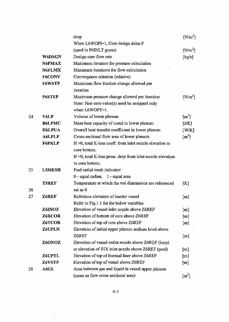
24
W6DSGNN6PMAXN6FLMXF6CONVF6WSTP
P6STEP
V6LPB6LPMCH6LPUAA6LPLFF6PKLP
25
2627
28
L5MESH
T5REF
Z6REF
Z6INOZZ6BCORZ6TCORZ6UPLN
Z6ONOZ
Z6UPTL
Z6VSTPA6GL
drop
When L6W0PI=l, Core design delta-P
(used in P6INLT guess)
Design core flow rate
Maximum iteration for pressure calculation
Maximum iterations for flow calculation
Convergence criterion (relative)
Maximum flow fraction change allowed per
iteration
Maximum pressure change allowed per iteration
Note: Non-zero value(s) need be assigned only
whenL6W0PT=l.
Volume of lower plenum
Mass heat capacity of metal in lower plenum
Overall heat transfer coefficient in lower plenum
Cross-sectional flow area of lower plenum
If >0, total K-loss coeff. from inlet nozzle elevation to
core bottom.
If <0, total K-loss press, drop from inlet nozzle elevation
to core bottom.
Fuel radial mesh indicator:
0 - equal radius, 1 - equal area
Temperature at which the rod dimensions are referenced
set as 0
Reference elevation of reactor vessel
Refer to Fig. 1.1 for the below variables
Elevation of vessel inlet nozzle above Z6REF
Elevation of bottom of core above Z6REF
Elevation of top of core above Z6REF
Elevation of initial upper plenum sodium level above
Z6REF
Elevation of vessel outlet nozzle above Z6REF (loop)
or elevation of IHX inlet nozzle above Z6REF (pool)
Elevation of top of thermal liner above Z6REF
Elevation of top of vessel above Z6REF
Area between gas and liquid in vessel upper plenum
(same as flow cross-sectional area)
[N/m2]
[N/m2]
[kg/s]
[N/m2]
[m3][J/K][W/K][m2]
[K]
[m]
[m][m][m]
[m]
[m][m][m]
[m2]
A-3

29
30
A6GM1 Area between gas and metal 1 in vessel upper plenum
A6GM2 Area between gas and metal 2 in vessel upper plenum
A6GM3 Area between gas and metal 3 in vessel upper plenum
A6LM1 Area between liquid and metal 1 in vessel upper plenum
A6LM2 Area between liquid and metal 2 in vessel upper plenum
A6 JET Area of core j et flow
H6GAS Heat transfer coeff. for cover gas in upper plenum
[W/Km2]
H6LNA Heat transfer coeff. at interface of two sodium zones
in upper plenum
H6INF Heat transfer coeff. at interface of two sodium zones
in upper plenum
Z6CHIM Length of chimney above core outlet
F6PKUP If >0, total K-loss coeff. from core top to outlet nozzle
elevation.
If <0, total K-loss P-drop from core top to outlet
nozzle elevation.
F6LEAK Fraction of bypass flow leaking directly into upper
plenum from lower bypass region
B6UMC1 Mass heat capacity of metal 1 in upper plenum
B6UMC2 Mass heat capacity of metal 2 in upper plenum
B6UMC3 Mass heat capacity of metal 3 in upper plenum
* See 3.1.3 Upper Plenum of SSC-K Manual for
descriptions of Metals 1, 2 and 3.
A6LFBP Flow area of lower region of bypass channel
A6UFBP Flow area of upper region of bypass channel
Y6LRBP Hydraulic diameter of lower bypass region channel
Y6URBP Hydraulic diameter of upper bypass region channel
F6INBP If >0, total K-loss coeff. at bypass inlet.
If <0, total K-loss P-drop at bypass inlet.
H6ABP Overall heat transfer coeff. between upper bypass
region sodium and liner
F6FRC1 Coeff. used in friction factor correlation for rod
bundles (Eq. 8-71)
F6FRC2 Coeff. used in friction factor correlation for rod
bundles (Eq. 8-71)
F6NUC1 Coeff. used in Nu number correlation (Forced
[m2]
[m2]
[m2]
[m2]
[m2]
[m2]
[W/Km2]
[W/Km2]
[m]
[N/m2]
[J/K]
[J/K]
[J/K]
[m2]
[m2]
[m]
[m]
[N/m2]
[W/K]
A-4
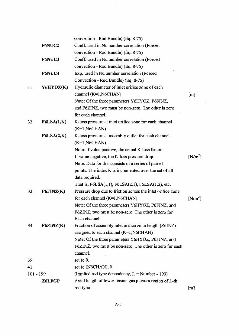
31
F6NUC2
F6NUC3
F6NUC4
Y6HYOZ(K)
32 F6LSA(1,K)
F6LSA(2,K)
33 P6FINZ(K)
34 F6ZINZ(K)
3941101 - 199
Z6LFGP
convection - Rod Bundle) (Eq. 8-75)
Coeff. used in Nu number correlation (Forced
convection - Rod Bundle) (Eq. 8-75)
Coeff. used in Nu number correlation (Forced
convection - Rod Bundle) (Eq. 8-75)
Exp. used in Nu number correlation (Forced
Convection - Rod Bundle) (Eq. 8-75)
Hydraulic diameter of inlet orifice zone of each
channel (K=1,N6CHAN) [m]
Note: Of the three parameters Y6HYOZ, P6FINZ,
and F6ZINZ, two must be non-zero. The other is zero
for each channel.
K-loss pressure at inlet orifice zone for each channel
(K=1,N6CHAN)
K-loss pressure at assembly outlet for each channel
(K=1,N6CHAN)
Note: If value positive, the actual K-loss factor.
If value negative, the K-loss pressure drop. [N/m2]
Note: Data for this consists of a series of paired
points. The index K is incremented over the set of all
data required.
That is, F6LSA(1,1), F6LSA(2,1), F6LSA(1,2), etc.
Pressure drop due to friction across the inlet orifice zone
for each channel (K=l ,N6CHAN) [N/m2]
Note: Of the three parameters Y6HYOZ, P6FINZ, and
F6ZINZ, two must be non-zero. The other is zero for
Each channel.
Fraction of assembly inlet orifice zone length (Z6INZ)
assigned to each channel (K=1,N6CHAN)
Note: Of the three parameters Y6HYOZ, P6FINZ, and
F6ZINZ, two must be non-zero. The other is zero for each
channel.
set to 0.
setto(N6CHAN),0
(Implied rod type dependency, L = Number - 100)
Axial length of lower fission gas plenum region of L-th
rod type [m]
A-5

Z6LBLK Axial length of lower blanket region of L-th rod type
Z6AFUL Axial length of active fuel region of L-th rod type
Z6UBLK Axial length of upper blanket region of L-th rod type
Z6UFGP Axial length of upper fission gas plenum region of L-th
rod type
N6LFGP Number of axial coolant nodes in lower fission gas
plenum region of L-th rod type
N6LBLK Number of axial coolant nodes in lower blanket region
of L-th rod type
N6AFUL Number of axial coolant nodes in active fuel region
of L-th rod type
N6UBLK Number of axial coolant nodes in upper blanket region
of L-th rod type
N6UFGP Number of axial coolant nodes in upper fission gas
plenum region of L-th rod type
F6PD Pitch to diameter ratio of L-th rod type
F6PWD Pitch to diameter ratio for wire wrap of L-th rod type
L5CLMT Index of cladding material of L-th rod type
L5STMT Index of structural material of L-th rod type
L5LBMT Index of lower blanket material of L-th rod type
F5DLBU Fractional unrestructured grain density of lower blanket
of L-th rod type
F5DLBE Fractional equiaxed grain density of lower blanket of
L-th rod type
F5DLBC Fractional columnar grain density of lower blanket of
L-th rod type
L5 AFMT Index of active fuel material of L-th rod type
F5D AFU Fractional unrestructured grain density of active fuel of
L-th rod type
F5DAFE Fractional equixed grain density of active fuel for L-th
rod type
F5DAFC Fractional columnar grain density of active fuel for L-th
rod type
L5UBMT Index of upper blanket material of L-th rod type
F5DTJBU Fractional unrestructured grain density of upper blanket
of L-th rod type
F5DXJBE Fractional equxiaxed grain density of upper blanket of
[m]
[m]
[m]
[m]
A-6

F5DUBC
N5ARODY5WIREY5FLATX5HXCNZ6INZ
201 - 299
F5PAX(J)
301 - 399
F5PRAD(I)
401 - 499
F5PWR5
F5PWR6
F5PWR1
501 - 599
L5GAS(I)F5GAS(I)
L-th rod type
Fractional columnar grain density of upper blanket of
L-th rod type
Number of rods per assembly of L-th rod type
Wire wrap diameter of L-th rod type
Hex-Can flat-to-flat inner diameter of L-th rod type
Total Hex-Can wall thickness of L-th rod type
Length of the inlet hydraulic orifice zone of L-th rod type
(Implied channel dependency, K = Number - 200)
Axial power fraction for each node in the K-th channel
(J=N5ASEC(L5ATYP(K)))
(Implied channel dependency, K = Number - 300)
Fuel power fraction in each radial fuel node iin the K-th
Channel (I=N5NFR(K))
Note: No axial dependence
(Implied channel dependency, K = Number - 400)
Fraction of power generated in the K-th channel deposited
directly into the fuel
Fraction of power generated in the K-th channel deposited
directly into the clad
Fraction of power generated in the K-th channel deposited
directly into the coolant
(Implied channel dependency, K = Number - 500)
Index of each fission gas type in the K-th chcinnel
Mole fraction of each fission gas in the K-th channel
Note: Data for this consists of a maximum of 3
paired points. The index I is incremented over the set
of all data required for the That is, L5GAS(1),
F5GAS(1), L5GAS(2), F5GAS(2), etc.
[m]
[m]
[m]
[m]
A-7

Sodium Loop Data (NALOOP)
Geometric and hydraulic data required to specify the primary and secondary
loop piping, pumps and IHX.
Rec. Variable1
100
101
N1LOOPN1PIPEN1NODE(J)
N2PIPEN2NODE(J)
F1LUMP(K)
N1TUBE
Y1TUB1Y1TUB2A1IHXV1BYPV1IHXB1SHELA1SHELF1PODH1FLPH1FLSL1STRCL1FDIR
L1KP
FUN
Description
Must be the first in file NALOOP
Number of primary loops simulated
Number of pipes in primary loop
Number of nodes in each pipe of primary loop
(J=1,N1PIPE)
Number of pipes in intermediate loop
Number of nodes in each pipe of intermediate loop
(J=1,N2PIPE)
Note: There exists an implied maximum number of
data elements for any record. At present this limit
is 99. This may restart the heat transport system
nodalization.
Number of actual loops in each simulated loop
(K=1,N1LOOP)
Number of tubes in IHX
Inner diameter of IHX tubes
Outer diameter of IHX tubes
Flow area on primary side of IHX
Volume of sodium in IHX primary bypass
Volume of sodium in IHX primary heat exchange region
Mass of IHX shell
Heat transfer area of IHX shell
Pitch-to-diameter ratio for IHX tube bundle
Fouling resistance on outer (primary) surface of tubes
Fouling resistance on inner (secondary) surface of tubes
Primary loop structural material ID
IHX flow indicator: 1 = parallel flow in IHX,
-1 = counter flow
Input option indicator: 0 = P1PDHX specified,
1 =F1LOSS(JIHX) specified
Primary inlet loss coefficient for IHX
Unit
[m]
[m]
[m2]
[m3]
[m3]
[kg][m2]
[m2K/W][m2K/W]
A-8
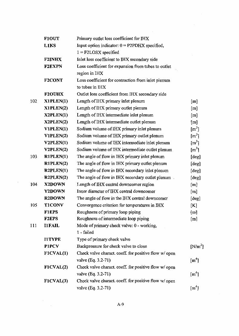
F1OUT Primary outlet loss coefficient for IHX
L1KS Input option indicator: 0 = P2PDHX specified,
1 = F2LOSX specified
F2INHX Inlet loss coefficient to IHX secondary side
F2EXPN Loss coefficient for expansion from tubes to outlet
region in IHX
F2CONT Loss coefficient for contraction from inlet plenum
to tubes in IHX
F2OUHX Outlet loss coefficient from IHX secondary side
102 XlPLEN(l) Length of IHX primary inlet plenum
XI PLEN(2) Length of IHX primary outlet plenum
X2PLEN(1) Length of IHX intermediate inlet plenum
X2PLEN(2) Length of IHX intermediate outlet plenum
VlPLEN(l) Sodium volume of IHX primary inlet plenum
V1PLEN(2) Sodium volume of IHX primary outlet plenum
V2PLEN(1) Sodium volume of IHX intermediate inlet plenum
V2PLEN(2) Sodium volume of IHX intermediate outlet plenum
103 Rl PLEN(l) The angle of flow in IHX primary inlet plenum
R1PLEN(2) The angle of flow in IHX primary outlet plenum
R2PLEN(1) The angle of flow in IHX secondary inlet plenum
R2PLEN(2) The angle of flow in IHX secondary outlet plenum .
104 X2DOWN Length of IHX central downcomer region
Y2DOWN Inner diameter of IHX central downcomer
R2DOWN The angle of flow in the IHX central downcomer
105 Tl CONV Convergence criterion for temperatures in IHX
F1EPS Roughness of primary loop piping
F2EPS Roughness of intermediate loop piping
111 I1FAIL Mode of primary check valve: 0 - working,
1 - failed
II TYPE Type of primary check valve
P1PCV Backpressure for check valve to close
FlCVAL(l) Check valve charact. coeff. for positive flow w/ open
valve (Eq. 3.2-71)
F1CVAL(2) Check valve charact. coeff. for positive flow w/ open
valve (Eq. 3.2-71)
Fl CVAL(3) Check valve charact. coeff. for positive flow w/ open
valve (Eq. 3.2-71)
[m]
[m]
[m]
[m]
[m3]
[m3]
[m3]
[m3]
[deg]
[deg]
[deg]
[deg]
[m]
[m]
[deg]
[K][m]
[m]
[N/m2]
[m4]
[m4]
[m4]
A-9
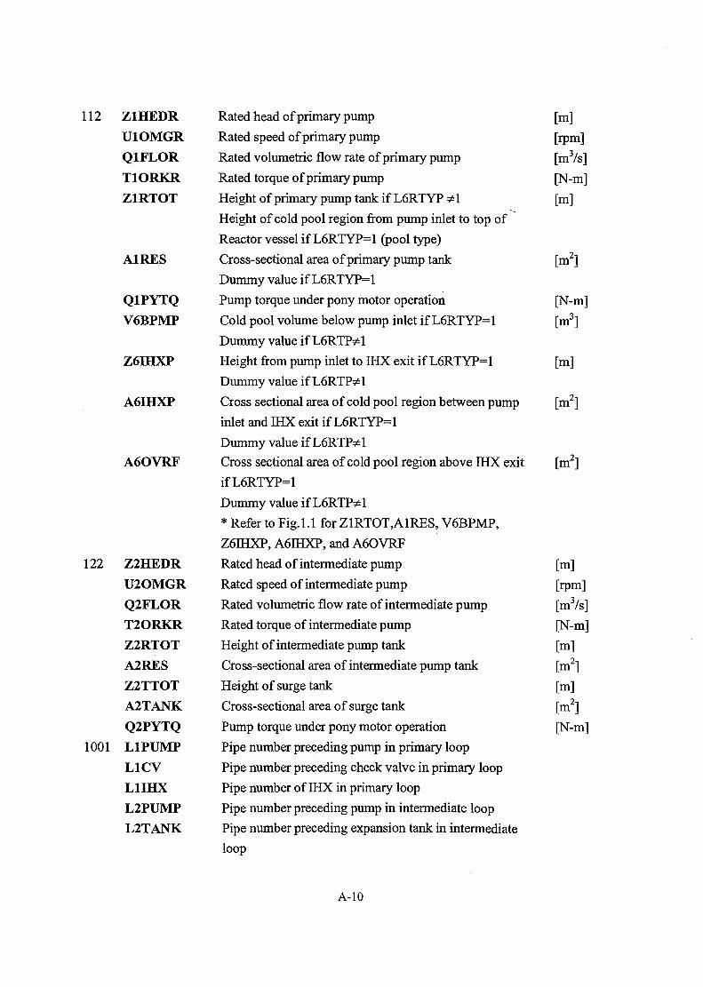
112 Z1HEDRU1OMGRQ1FLORT1ORKRZ1RTOT
AIRES
Q1PYTQV6BPMP
Z6IHXP
A6IHXP
A6OVRF
122 Z2HEDRU2OMGRQ2FLORT2ORKRZ2RTOTA2RESZ2TTOTA2TANKQ2PYTQ
1001 L1PUMPL1CVL1IHXL2PUMPL2TANK
Rated head of primary pump
Rated speed of primary pump
Rated volumetric flow rate of primary pump
Rated torque of primary pump
Height of primary pump tank if L6RTYP *1
Height of cold pool region from pump inlet to top of
Reactor vessel if L6RTYP=1 (pool type)
Cross-sectional area of primary pump tank
Dummy value if L6RTYP=1
Pump torque under pony motor operation
Cold pool volume below pump inlet if L6RTYP=1
Dummy value if L6RTP*1
Height from pump inlet to IHX exit if L6RTYP=1
Dummy value if L6RTP*1
Cross sectional area of cold pool region between pump
inlet and IHX exit if L6RTYP=1
Dummy value if L6RTP*1
Cross sectional area of cold pool region above IHX exit
ifL6RTYP=l
Dummy value if L6RTP*1
* Refer to Fig. 1.1 for Z1RTOT,A1RES, V6BPMP,
Z6IHXP, A6IHXP, and A6OVRF
Rated head of intermediate pump
Rated speed of intermediate pump
Rated volumetric flow rate of intermediate pump
Rated torque of intermediate pump
Height of intermediate pump tank
Cross-sectional area of intermediate pump tank
Height of surge tank
Cross-sectional area of surge tank
Pump torque under pony motor operation
Pipe number preceding pump in primary loop
Pipe number preceding check valve in primary loop
Pipe number of IHX in primary loop
Pipe number preceding pump in intermediate loop
Pipe number preceding expansion tank in intermediate
loop
[m]
[rpm]
[m3/s]
[N-m]
[m]
[m2]
[N-m]
[m3]
[m]
[m2]
[m2]
[m]
[rpm]
[m3/s]
[N-m]
[m]
[m2]
[m]
[m2]
[N-m]
A-10

L2SG1002 F1BETA
N1ACTVP1PDHX
10003 P2PDHXF2LOSX
1101-1199
F1LOSSX1PIPEY1PIPE
Y1THIK
R1SIN(I)
1201 - 1299
F2LOSS
X2PIPEY2PIPEY2THIKR2SIN(I)
Pipe number preceding evaporator in intermediate loop
Primary bypass fraction through IHX
Number of active (unplugged) tubes in IHX of loop
Pressure drop over IHX primary side
Pressure drop over secondary side of IHX
Loss coefficient for secondary side of IHX
(Implied (Primary loop) pipe dependency,
J = Number -1100)
Loss coefficient for J-th pipe in primary loop
Length of J-th pipe in primary loop
Inner diameter of J-th pipe in primary loop
Note: For IHX, enter primary side hydraulic diameter.
Thickness of J-th pipe wall in primary loop
Note: This value is ignored for IHX primary pipe.
Angle of primary flow at each node in J-th pipe
of loop (I = 1,N1NODE(N1PIPE(J)))
(Implied (Intermed. loop) pipe dependency,
J = Number-1200)
Loss coefficient for J-th pipe in intermediate loop
Length of J-th pipe in intermediate loop
Inner diameter of J-th pipe in intermediate loop
Thickness of J-th pipe wall in intermediate loop
Angle of intermediate flow at each node of J-th pipe
of loop (1=1, N2NODE(N2PIPE(J)))
[N/m2]
[N/m2]
[m]
[m]
[m]
[deg]
[m]
[m]
[mj
[deg]
A-ll

MINET DATA (MINETD)
Steam Generator and Balance of Plant Data. All data required to specify the steam
generator system (including balance of plant) and its associated sodium-side interfaces.
Rec. Variable
1
101
201
MODIDINLETIDOUTLETIDX3MODY3IDE3PSIN3NODEN3PATH
MODIDINLETIDOUTLETIDX3MODY3ID
E3PSIN3NODEN3PATHA3VMAXS3VMINF3STOA
MODIDINLETIDOUTLETIDX3MODY3IDE3PSIN3NODEN3PATH
Description
301
Pipe Geometric
Module ID assigned to pipe
Port identifier assigned to inlet port
Port identifier assigned to outlet port
Length of module
Diameter of module
Surface roughness factor, roughness/surface
Number of nodes to be used for module
Number of parallel units being represented
Valve Geometric
Module ID assigned to valve
Port identifier assigned to inlet port
Port identifier assigned to outlet port
Length of module (Pipe-like portion)
Diameter of module (Pipe-like portion)
Surface roughness factor, roughness/surface
For valve, must use 1 node
Number of parallel units being represented
Maximum flow area thru valve when open
Minimum valve position, relative, must be GT 0.0
Factor, position to area, AREA=POSITN**F3STOA
Pump Geometric
Module ID assigned to pump
Port identifier assigned to inlet port
Port identifier assigned to outlet port
Length of module (Pipe-like portion)
Diameter of module (Pipe-like portion)
Surface roughness factor, roughness/surface
Number of nodes, for pump use 1 node
Number of parallel units being represented
Heat exchanger geometric
Unit
[m][m]
[m][m]
[m2]
[m][m]
A-12
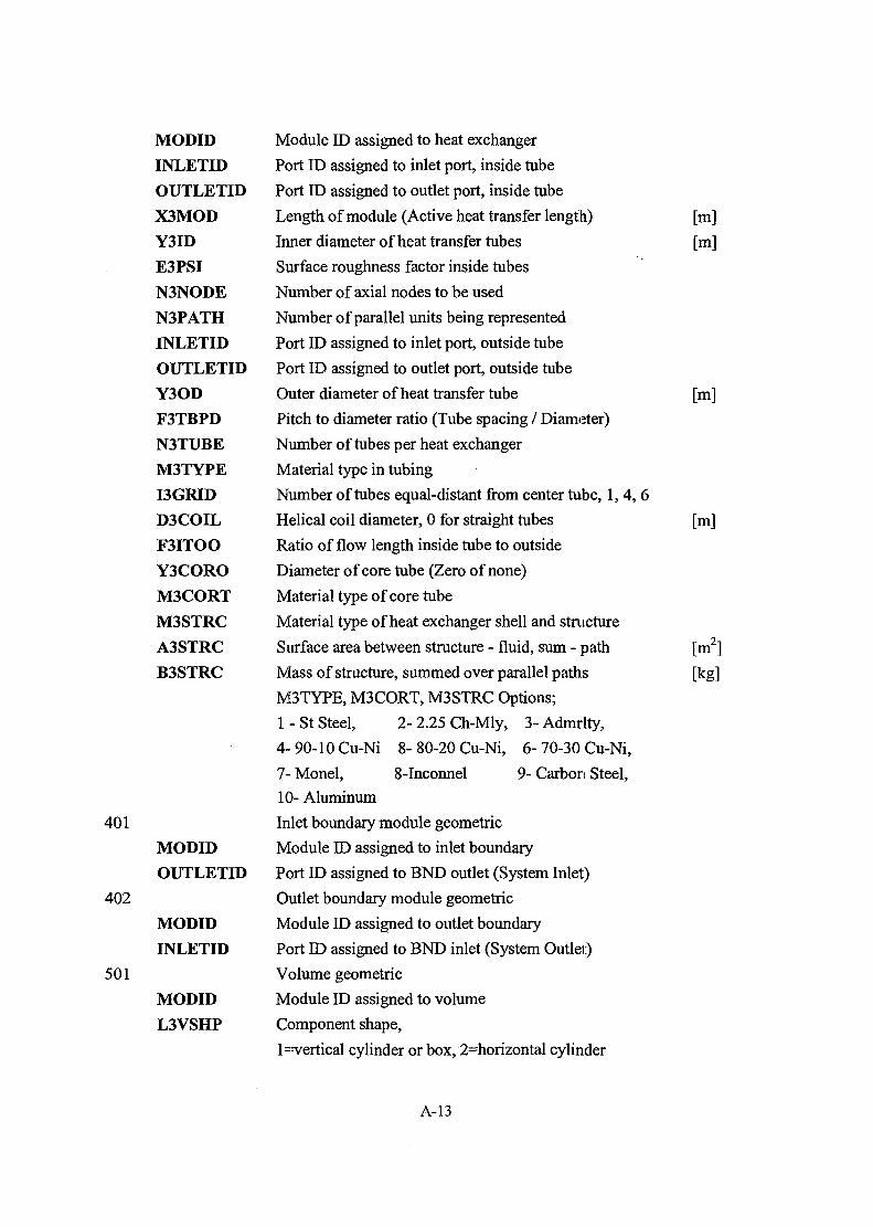
401
402
501
MODID Module ID assigned to heat exchanger
INLETID Port ID assigned to inlet port, inside tube
OUTLETID Port ED assigned to outlet port, inside tube
X3MOD Length of module (Active heat transfer length)
Y3ID Inner diameter of heat transfer tubes
E3PSI Surface roughness factor inside tubes
N3NODE Number of axial nodes to be used
N3PATH Number of parallel units being represented
INLETID Port ID assigned to inlet port, outside tube
OUTLETID Port ID assigned to outlet port, outside tube
Y3OD Outer diameter of heat transfer tube
F3TBPD Pitch to diameter ratio (Tube spacing / Diameter)
N3TUBE Number of tubes per heat exchanger
M3TYPE Material type in tubing
I3GRID Number of tubes equal-distant from center tube, 1,4, 6
D3COIL Helical coil diameter, 0 for straight tubes
F3ITOO Ratio of flow length inside tube to outside
Y3CORO Diameter of core tube (Zero of none)
M3CORT Material type of core tube
M3STRC Material type of heat exchanger shell and structure
A3STRC Surface area between structure - fluid, sum - path
B3STRC Mass of structure, summed over parallel paths
M3TYPE, M3C0RT, M3STRC Options;
1 - St Steel, 2- 2.25 Ch-Mly, 3- Admrlty,
4- 90-10 Cu-Ni 8- 80-20 Cu-Ni, 6- 70-30 Cu-Ni,
7- Monel, 8-Inconnel 9- Carbon Steel,
10-Aluminum
Inlet boundary module geometric
MODID Module ID assigned to inlet boundary
OUTLETID Port ID assigned to BND outlet (System Inlet)
Outlet boundary module geometric
MODID Module ID assigned to outlet boundary
INLETID Port ID assigned to BND inlet (System Outlet)
Volume geometric
MODID Module ID assigned to volume
L3VSHP Component shape,
l=vertical cylinder or box, 2=horizontal cylinder
[m]
[m]
[m]
[m]
[m2]
[kg]
A-13

V3VOL Volume within module (Portion of component) [m3]
Y3VOL Total height of component [m]
F3 VMIN Relative height of module low point with respect to
component
F3VMAX Relative height of module high point with respect to
component
Z3VOL Elevation of component vertical midpoint [m]
N3PATH Number of parallel units being represented
L3PSEP l=homogeneous, 2=separated phases, 3=1 SS-2TRN
511 Volume inlet port geometric
MODID Module ID assigned to volume
INLETID Port ID assigned to incoming volume port
512 Volume outlet port geometric
MODID Module ID assigned to volume
OUTLETID Port ID assigned to outgoing volume port
601 Turbine stage geometric
MODID Module ID assigned to turbine stage
INLETID Port ID assigned to inlet port
OUTLETID Port ID assigned to outlet port
ALPHA Absolute angle of approach steam with respect to
blade, eg-15 [deg]
801 Network geometric
MODID Module ID of any boundary or accumulator in network
IFTYPN Fluid type, 1-H2O, 2-Sodium, 3-Air, 4-NaK
901 Junction
Z3 J CTN Elevation of interface between module ports [m]
MODID1 Module ID of first module
PORTID1 Port ID of first module
MODID2 Module ID of second module
PORTID2 Port ID of second module
1001 Pipe performance
MODID Module ID of pipe
F3KMI Loss coefficient (K) for module
1101 Valve performance (If choked, must isolate)
MODID Module ID of valve
F3KMI Module loss coefficient - pipe-like section
F3VALV Loss coefficient across valve opening
A-14

I3CHOK Choke flow option, 0-none, 1-choking expected
J3VPRS Volume where pressure taken, not used= -999
P3VOPN Pressure at which valve trips open [Pa]
S3VOPN Valve opening time constant [s]
P3VCLO Pressure at which valve trips shut [Pa]
S3VCLO Valve closing time constant [s]
** Alternate use of last parameters ** For check valve
J3VPRS=0 for check valve
P3VOPN=flow/path [kg/s] to open
P3VCLOflow/path [kg/s] to close
1201 Pump performance
MODID Module ID of pump
F3KMI Module loss coefficient
W3REFF Reference flow rate (per unit) [kg/s]
H3REF Reference pump head [m]
F3REF Reference pump speed [rpm]
A3PUMP (1) HEAD(SPEED,FLOW)=H3REF*(SPEED/F3REF)**2
(2) *(A3PUMP(1)+A3PUMP(2)*WRATIO
(3)+A3PUMP(3)*WRATIO**2+A3PUMP(4)*WRATIO**3
(4) +A3PUMP(5)*WRATIO**4)
(5) where WRATIOW/(W3REFF*(SPEED/F3REF))
S3PTAU Pump coastdown time constant, SPD=SPD0*E-T/TAU [s]
S3PSEZ Pump seizure time after trip [s]
1301 Heat exchanger performance
MODID Module ID of heat exchanger
F3KMI Module loss coefficient, inside tubes
F3KMO Module loss coefficient, outside tubes
I3LVTI DNB/DRYOUT option,
1-DNB, 2-DRYOUT, 3-X=0.75
I3LVTO Same as I3LVTI, but applied outside tubes
F3CCFL Flow direction, l=parallel, 0=cross, -l=counter
1601 Turbine performance
MODID Module ID for turbine
I3TTYP Turbine stage type, l=impulse, 2=impuls-react
E3FGEN Efficiency to electrical grid
W3TREF Reference flow rate [kg/s]
P3ITRF Reference inlet pressure [Pa]
A-15

P3OTRF Reference outlet pressure
T3ITRF Reference inlet temperature
R3TSRF Reference speed
S3TTAU Coastdown time constant, SPD=SPDO*EXP(-T/TAU)
S3TSEZ Seizure time (After Trip)
2001 Pipe initial condition (All QMOD's subject to adjust.)
MODID Module ID of pipe
Q3MOD Heat put into module, sum over parallel units
2101 Valve initial condition
MODID Module ID of valve
Q3MOD Heat put into module, sum over parallel units
S3VPOS Initial stem position, relative, 0=closed, l=open
2201 Pump initial condition
MODID Module ID of pump
Q3MOD Heat put into module, sum over parallel units
F3PUMP Initial pump speed
2301 Heat exchanger initial condition
MODID Module ID of heat exchanger
Q3MOD Total heat transfer, out to in, sum over parallel units
2401 Boundary module initial condition
MODID Module ID of boundary
K3EBST Boundary status, 0=inlet, l=floating, 2=fixed
K3EBC E3BC flag, l=enthalpy, 2=temperature, 3=quality
E3BC Enthalpy, temperature, or quality (If H2O)
W3BC Mass flow (total) used for inlets only
P3BC Pressure used for outlets only
2501 Volume initial condition
MODID Module ID of volume
Q3MOD Heat put into module, sum over parallel units
F3LQLV Relative liquid level vs component height
P3VOL Estimated volume pressure at steady state
2511 Volume outlet port initial condition
MODID Module ID of volume
OUTLETID Outlet port ID of volume
W3VOUT Estimate of flow exiting, sum over parallel path
2601 Turbine stage initialization
[Pa]
[K]
[rpm]
[s]
[J/s]
[J/s]
[J/s]
[J/s]
[J/KG]
or [K]
[kg/s]
[Pa]
[J/s]
[Pa]
A-16
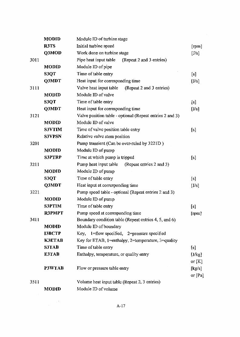
MODID Module ID of turbine stage
R3TS Initial turbine speed
Q3MOD Work done on turbine stage
3011 Pipe heat input table (Repeat 2 and 3 entries)
MODID Module ID of pipe
S3QT Time of table entry
Q3MDT Heat input for corresponding time
3111 Valve heat input table (Repeat 2 and 3 entries)
MODID Module ID of valve
S3QT Time of table entry
Q3MDT Heat input for corresponding time
3121 Valve position table - optional (Repeat entries 2 and 3)
MODID Module ID of valve
S3VTIM Time of valve position table entry
S3VPSN Relative valve stem position
3201 Pump transient (Can be over-ruled by 3221D)
MODID Module ID of pump
S3PTRP Time at which pump is tripped
3211 Pump heat input table (Repeat entries 2 and 3)
MODID Module ID of pump
S3QT Time of table entry
Q3MDT Heat input at corresponding time
3221 Pump speed table - optional (Repeat entries 2 and 3)
MODID Module ID of pump
S3PTIM Time of table entry
R3PMPT Pump speed at corresponding time
3411 Boundary condition table (Repeat entries 4,5, and 6)
MODID Module ID of boundary
I3BCTP Key, l=flow specified, 2=pressure specified
K3ETAB Key for ETAB, l=enthalpy, 2=temperature, 3=quality
S3TAB Time of table entry
E3TAB Enthalpy, temperature, or quality entry
P3WTAB Flow or pressure table entry
3511 Volume heat input table (Repeat 2, 3 entries)
MODID Module ID of volume
[rpm][J/s]
[J/s]
[s][J/s]
[s]
[s]
[s][J/s]
[s][rpm]
[s][J/kg]
or[K]
[kg/s]
or [Pa]
A-17

S3QT Time of table entry [s]
Q3MDT Heat input at corresponding time [J/s]
3601 Turbine trip (Can be overruled by 361 ID )
MODID Module ID of turbine stage
S3TSTP Turbine trip time [s]
3611 Turbine speed table - optional (Repeat entries 2 and 3)
MODID Module ID of turbine stage
S3TSTB Time of turbine speed table entry [s]
R3TSTB Turbine speed at corresponding time [rpml
4000 Run control card
S3END End of transient simulation [s]
4100 Print control (Repeat entries 3 and 4)
L3PRON Step number to start frequent prints, -1 for SS
L3PRNT Keys print detail, l=brief, 2=middle, 3=detailed
S3PRIN Print interval [s]
S3PLIM Time limit for corresponding print mterval value [s]
4200 Context save control
L3REST Context restore control,
0=no restore, l=restore context
N3SINT Context save control, defines print count between saves
A-18

OPDATA
Initial overall plant operating conditions and specification of plant
balance initialization logic.
Rec. Variable Description
1 P9OPN9LOOP
2 T6OUTLT6INLT
W1LOOP
T2IHXIT2IHXOW2LOOP
P1GASIP2GASIZ2TANKT1PUMPT2PUMPL1EPRT
Reactor power
Number of operating loops present in plant
Vessel sodium outlet temperature
Vessel sodium inlet temperature
cf. TRNDAT 8015, T81REF
Sodium flow rate in primary loop
cf. TRNDAT 8015, W81REF
Note: Of the three parameters in this, two must be
specified as known (denoted by entering values greater
than zero) while the other one is assumed unlmown
(denoted by entering a value less than zero) aid will be
calculated by SSC. The unknown value to be entered
need not be too precise; it can be an approximate initial
guess.
IHX intermediate sodium inlet temperature
IHX intermediate sodium outlet temperature
Sodium flow rate in intermediate loop
cf. TRNDAT 8015, W82REF
Note: Of the three parameters in this one must be
specified as known (denoted by entering values greater than
zero) while the others are assumed unknown (denoted by
entering a value less than zero) and will be calculated by
SSC. The accuracy of the initial guesses for this
are more important.
Initial cover gas pressure in each primary pump tank
Initial cover gas pressure in each intermediate loop
Height of coolant in surge (expansion) tank
Temperature rise across primary pump
Temperature rise across intermediate pump
Primary and intermediate loop detailed print option;
1= report, 0= no report
Unit[W]
[K]
[K]
[kg/s]
[K]
[K]
[kg/s]
[N/m2]
[N/m2]
[m]
[K]
[K]
A-19

L3PRNT SG detailed print option;
1 - 4 = low to high detail report,
0 = no report
L5PRNT Detailed in vessel temp, distribution print option;
1 = report, 0 = no report
L6PRNT In-vessel fluid dynamics detailed print option;
1 = report, 0 = no report
A-20

MATDAT
A set of material properties data is built into the code. The data required to
alter the default values of the material properties, or to create new material
properties, are input to the code through data file MATDAT.
Rec. Variable10
40-49
50-59
60-69
70-79
80-89
TRNDAT
Rec.
1001
1002
1003
Variable
LIPONY(K)
F1PONYQ1NRTAL2PONY(K)
F2PONYQ2NRTAL1GV(K)
V1MINRZ1MAXR
F1GVR(1)F1GVR(2)F1GVR(3)V1MINP
Description
Material properties for sodium
Material properties for blanket
Material properties for fuel
Material properties for cladding
Material properties for structural material
Material properties for cover gas
Transient scenario data
DescriptionPrimary loop pony motor status;
1 = motor is on, 0 = motor is off (K = 1,N1LOOP)
Primary pony motor speed fraction of rated speed
Primary pump inertia [KG*M2]
Secondary loop pony motor status;
1 = motor is on, 0 = motor is off ( K - 1.N1LOOP )
Secondary pony motor speed fraction of rated speed
Secondary pump inertia
Guard vessel option;
0 = no guard vessel, 1 = reactor vessel outlet,
2 = RV inlet, 3 = pump inlet, 4 = pump outlet,
5 = IHXinlet, 6 = IHX outlet (K=1,N1LOOP)
R. V. guard vessel volume at level with break
R. V. guard vessel maximum level that can be reached
by coolant
R. V. guard vessel volume to level coeff.
R.V. guard vessel volume to level coeff.
R.V. guard vessel volume to level coeff.
Pump guard vessel volume at level with pipe break
Unit
Unit
[kg,m2]
[m3]
[m]
[m3]
A-21
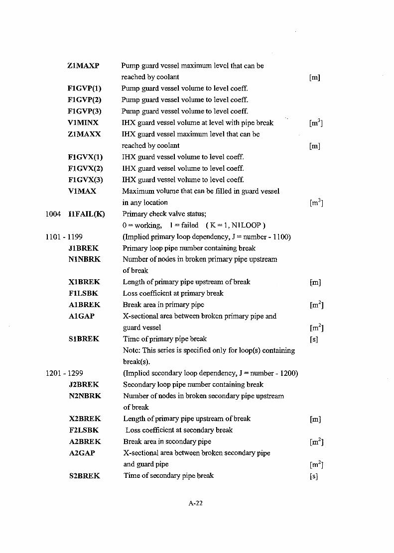
Z1MAXP
FlGVP(l)F1GVP(2)F1GVP(3)V1MINX
Z1MAXX
FlGVX(l)F1GVX(2)F1GVX(3)V1MAX
1004 I1FAIL(K)
1101-1199J1BREKN1NBRK
X1BREKF1LSBKA1BREKA1GAP
S1BREK
1201 - 1299J2BREKN2NBRK
X2BREKF2LSBKA2BREKA2GAP
S2BREK
Pump guard vessel maximum level that can be
reached by coolant
Pump guard vessel volume to level coeff.
Pump guard vessel volume to level coeff.
Pump guard vessel volume to level coeff.
IHX guard vessel volume at level with pipe break
IHX guard vessel maximum level that can be
reached by coolant
IHX guard vessel volume to level coeff.
IHX guard vessel volume to level coeff.
IHX guard vessel volume to level coeff.
Maximum volume that can be filled in guard vessel
in any location
Primary check valve status;
0 = working, 1= failed (K=1,N1LOOP)
(Implied primary loop dependency, J = number - 1100)
Primary loop pipe number containing break
Number of nodes in broken primary pipe upstream
of break
Length of primary pipe upstream of break
Loss coefficient at primary break
Break area in primary pipe
X-sectional area between broken primary pipe and
guard vessel
Time of primary pipe break
Note: This series is specified only for loop(s) containing
break(s).
(Implied secondary loop dependency, J = number -1200)
Secondary loop pipe number containing break
Number of nodes in broken secondary pipe upstream
of break
Length of primary pipe upstream of break
Loss coefficient at secondary break
Break area in secondary pipe
X-sectional area between broken secondary pipe
and guard pipe
Time of secondary pipe break
[m]
[m3]
[m]
[m3]
[m]
[m2]
[m2]
[s]
[m]
[m2]
[m2]
[s]
A-22

3101 MODIDN3TABI3BCTP
3111 MODIDS3TAB(I)E3TAB(I)P3WTAB(I)
3201 MODIDN3VOLT
3211 MODID
S3VOLT(I)Q3VOLT(I)
3301 MODIDN3VALT(I)
N3VCAS
3311 MODIDS3VALT(I)S3VPST(I)
3401 MODIDN3PUMT(I)S3PTRPN3PCAS
3411 MODIDS3PUMT(I)R3PUMT(I)
Note: This series is specified only for loop(s)
containing break(s).
Module ID of boundary
Number of table entries on corresponding 3111
Boundary condition type; 1 = flow, 2 = pressure
Module ID of boundary
Time for table entry [s]
Enthalpy [J/KG] or temperature [K] for table entry
Pressure [Pa] of flow [kg/s] for table entry
Note: Data is entered as a user defined series
of paired points.
Module ID of volume (Accumulator)
Number of table entries on corresponding 3211
Module ID of volume
Time for table entry [s]
Heat input to all parallel volumes [J/s]
Note: Data is entered as a user defined series of
paired points.
Module ID of valve
Number of table entries on corresponding 3311
PPS/PCS option;
0 = Ignore PPS/PCS, 1 = Accept PPS/PCS signal
Note: At present, N3VCAS must be set equal to zero.
Module ID of valve
Time for table entry [s]
Valve stem position; 0 = Full closed, 1 = Full open
Note: Data is entered as a user defined series of
paired points.
Module ID of pump
Number of table entries on corresponding 3411
Pump trip time [s]
PPS/PCS option;
0 = Ignore PPS/PCS, 1 = Accept PPS/PCS sigaal
Note: At present, N3PCAS must be set equal to zero.
Module ID of pump
Time for table entry [s]
Relative pump speed; 0 = Full stop, 1 = Full speed
A-23

5001 L5POPT
N5DNGPC5LN
5002 F5PFIS(K)
5003 F5BETA(N)
5004 C5LMDA(N)
5005 F5PBPD(I)S5PBPD(I)
5101-5199F5PD(I)S5PD(I)
5201 - 5299
F5BDOP(J)
5301 - 5399
F5GDOP(J)
5401 - 5499
F5VWGT(J)
5501 - 5599
F5AWGT(J)
6001 L6MIX
Note: Data is entered as a user defined series of
paired points.
Transient power flag;
0 = Prompt jump approximation, 1 = exact
Number of delayed neutron groups (Maximum of 6)
Prompt neutron generation time [s]
Fractional power in each channel and bypass due to
fission heating (K = 1,N6CHAN+1 )
Fraction of N-th effective delayed neutron group
(0<N<7)
Decay constant of N-th delayed neutron group
(0<N<7)
Fractional transient decay power in bypass
Transient postscram time for decay power in bypass [s]
Note: Data is assigned as a user defined series of paired
points of up to 25 pairs
(Implied channel dependency, K= Number - 5100)
Fractional transient decay power in K-th channel
Transient postscram time for decay power in K-th
channel [s]
Note: Data is assigned as a user defined series of paired
points of up to 25 pairs
(Implied channel dependency, K= Number - 5200)
Mesh weighted Doppler reactivity coefficient with sodium
present for K-th channel (J=l ,N5SLIC(K)) [p]
(Implied channel dependency, K= Number - 5300)
Mesh weighted Doppler reactivity coefficient w/o sodium
present for K-th channel (J=l,N5SLIC(K)) [p]
(Implied channel dependency, K= Number - 5400)
Mesh weighted sodium void reactivity coefficient for
K-th channel (J=l ,N5SLIC(K)) [p/kg]
(Implied channel dependency, K= Number - 5500)
Mesh weighted fuel axial expansion reactivity
coefficient for K-th channel [p/kg]
(J=1,N5SLIC(K))
Upper Plenum Mixing type option;
1= one zone mixing, 2= two zone mixing
A-24

L6FLOW
T6SUPH
6002 L6CGAS
Q6CGFBP6CGFB
8001 N8PCSD
N8CBNK8002 L8PUMP(J)
8003 S8TDLY(J)
Flow redistribution option; 0 = No flow redistribution,
1 = Flow redistribution
Super heat temperature
If set XT. 0.0, thermal expansion model will be used in
boiling calculations.
If set .GE. 0.0, single mass flow rate will be used in
boiling calculations.
Cover gas pressure option;
1 = constant mass, 2 = constant pressure
3 = constant feed/bleed rate
Cover gas feed/bleed rate
Cover gas pressure change required to actuate
feed/bleed valve
Number of feedback cascades in the reactor
power controller
Number of primary control rod banks
Manual/Auto pump trip flag;
1 = manual, 0 = auto (J=1,(4*N1LOOP+1))
Note: Parameters are assigned on a subsystem/component
basis. That is, data assignments are made for the pump in
primary loop 1, the pump in primary loop 2 (if needed), and
so on, up to the pump in primary loop "NILOOP". The data
for all "NILOOP" primary loop pumps is followed by
corresponding series for the secondary loop(s) and each of
two dummy steam generator pumps. Data for the last pump is
assigned to the turbine. Pump trips for the steam generator
and turbine must be set through RECORD 3401.
Pump trip time delay after an automatic PPS signal [s]
(J=1,(4*N1LOOP+1))
Note: Parameters are assigned on a subsystem and
component basis.
That is, data assignments are made for the pump in primary
loop 1, the pump in primary loop 2 (if needed), and so on,
up to the pump in primary loop "NILOOP". The data for all
"NILOOP" primary loop pumps is followed by corresponding
series for the secondary loop(s) and each of two dummy steam
generator pumps. Data for the last pump is assigned to the
[kg/s]
[N/m2]
A-25

8004 S8MANP(J)
8005 F8PD1F8PD2S8DT1S8DT2
8006 F8RSCR
F8RSDM
Z8SRMX
F8SRMX
F8RSTP
F8RSTS
8007 C8A0C8A1C8A2C8A3C8A4C8A5
turbine. Pump trips for the steam generator and turbine
must be set through RECORD 3401.
Time at which pumps are to be tripped manually [s]
(J=1,(4*N1LOOP+1)) and time at which IHX are to be
isoltaed manually
* Note: Parameters are assigned on a subsystem/component
basis. That is, data assignments are made for the pump
in primary loop 1, the pump in primary loop 2 (if needed),
and so on, up to the pump in primary loop "N1LOOP".
The data for all "N1LOOP" primary loop pumps is
followed by corresponding series for the secondary
loop(s) and each of two dummy steam generator pumps
Data for the last pump is assigned to the turbine.
Pump trips for the steam generator and turbine must be
set through RECORD 3401.
Fractional power demand at time S8DT1
Fractional power demand at time S8DT2
Time at which the load demand starts changing [s]
Time at which the load demand reaches a constant level [s]
Reactivity worth due the secondary control rods
(Eq. 3.4-30) [$]
Cold shutdown margin of reactivity (Constant)
(Eq. 3.4-30) [$]
Maximum insertion limit of the secondary control
rods corresponding to F8SRMX (Eq. 3.4-31) [m]
Maximum reactivity worth of the secondary control
rods (Eq. 3.4-31) [$]
Reactivity worth of the primary system stuck rod
(Eq. 3.4-38A) [$]
Reactivity worth of the secondary system stuck rod
(Eq. 3.4-38B) [$]
Coefficients for a 6th degree polynomial (Eq. 3.4-37)*
Coefficients for a 6th degree polynomial (Eq. 3.4-37)*
Coefficients for a 6th degree polynomial (Eq. 3.4-37)*
Coefficients for a 6th degree polynomial (Eq. 3.4-37)*
Coefficients for a 6th degree polynomial (Eq. 3.4-37)*
Coefficients for a 6th degree polynomial (Eq. 3.4-37)*
A-26
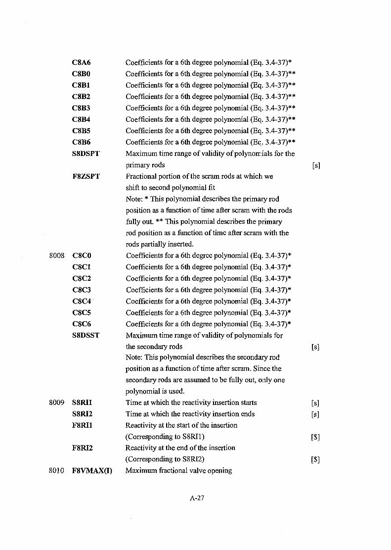
C8A6
C8B0
C8B1
C8B2
C8B3
C8B4
C8B5
C8B6
S8DSPT
F8ZSPT
8008 C8C0
C8C1
C8C2
C8C3
C8C4
C8C5
C8C6
S8DSST
8009 S8RI1S8RI2F8RI1
F8RI2
8010 F8VMAX(I)
Coefficients for a 6th degree polynomial (Eq. 3.4-37)*
Coefficients for a 6th degree polynomial (Eq. 3.4-37)**
Coefficients for a 6th degree polynomial (Eq. 3.4-37)**
Coefficients for a 6th degree polynomial (Eq. 3.4-37)**
Coefficients for a 6th degree polynomial (Eq. 3.4-37)**
Coefficients for a 6th degree polynomial (Eq. 3.4-37)**
Coefficients for a 6th degree polynomial (Eq. 3.4-37)**
Coefficients for a 6th degree polynomial (Eq. 3.4-37)**
Maximum time range of validity of polynomials for the
primary rods [s]
Fractional portion of the scram rods at which we
shift to second polynomial fit
Note: * This polynomial describes the primary rod
position as a function of time after scram with the rods
fully out. ** This polynomial describes the primary
rod position as a function of time after scram with the
rods partially inserted.
Coefficients for a 6th degree polynomial (Eq. 3.4-37)*
Coefficients for a 6th degree polynomial (Eq. 3.4-37)*
Coefficients for a 6th degree polynomial (Eq. 3.4-37)*
Coefficients for a 6th degree polynomial (Eq. 3.4-37)*
Coefficients for a 6th degree polynomial (Eq. 3.4-37)*
Coefficients for a 6th degree polynomial (Eq. 3.4-37)*
Coefficients for a 6th degree polynomial (Eq. 3.4-37)*
Maximum time range of validity of polynomials for
the secondary rods [s]
Note: This polynomial describes the secondary rod
position as a function of time after scram. Since the
secondary rods are assumed to be fully out, only one
polynomial is used.
Time at which the reactivity insertion starts [s]
Time at which the reactivity insertion ends [s]
Reactivity at the start of the insertion
(Corresponding to S8RI1) [$]
Reactivity at the end of the insertion
(Corresponding to S8RI2) [$]
Maximum fractional valve opening
A-27

F8TRMA(I)
8011 F8VMIN(I)
F8TRMN(I)
8012 S8OPEN(I)
8013 S8CLOS(I)
8014 C8TIME(I)
8015 U81REF
(I=l,(NlLOOP+3)) (Eq. 3.4-57)*
Maximum valve trim (I=l,(NlLOOP+3)) (Eq. 3.4-57)*
Note: * Data is entered as a series of paired points.
The index "I" is incremented over the set of all required
data. The required valve sequencing is:
Main feed water control valve (one entry per loop)
Throttle valve, Bypass valve, Motor operated relief valve
Minimum fractional valve opening
(I=l,(NlLOOP+3)) (Eq. 3.4-57)*
Minimum valve trim (I=l,(NlLOOP+3))
(Eq. 3.4-57)*
Note: * Data is entered as a series of paired points.
The index "I" is incremented over the set of all required
data. The req uired valve sequencing is:
Main feed water control valve (one entry per loop)
Throttle valve, Bypass valve, Motor operated relief valve
Valve opening time (1=1 ,(NlLOOP+3))
(Eq. 3.4-57)
Note: The required valve sequencing is:
Main feed water control valve (one entry per loop)
Throttle valve, Bypass valve, Motor operated relief valve
Valve closing time (I=l,(NlLOOP+3)) (Eq. 3.4-57)
Note: The required valve sequencing is:
- Main feed water control valve (one entry per loop)
- Throttle valve, Bypass valve, Motor operated relief valve
Time constants used in computing sensor measurement
time lags (I=1,3+5*N1LOOP)
Note: These constants correspond to the following sensors:
- Reference pressure
- Sodium level
- IHX outlet temperature (one entry per loop)
- Evaporator inlet temperature (one entry per loop)
- Feed water flow rate (one entry per loop)
- Steam flow rate (one entry per loop)
- Steam drum level (one entry per loop)
- Reactor outlet nozzle temperature
Refence 100 % power, primary loop pump speed
[s]
[s]
[s]
A-28

U82REFW81REF
W82REF
T8RREF
T81REF
T8TREFP86REFP8TREFP8DPRF
W8FWRFW8STRF
8016 L8AVLP(I)
8017 L8AVLS(I)
8018 L8FUNP(I)
8019 L8FUNS(I)
8020 L8PMAN
S8PDLY
S8PMAN
8021 L8SMAN
Reference 100 % power, intermediate loop pump speed
Reference 100 % power, primary loop sodium mass
flow rate, cf. OPDATA 2, W1LOOP
Reference 100 % power, intermediate loop sodium mass
Flow rate, cf. OPDATA 3, W2LOOP
Reference 100 % power, core mixed mean outlet
temperature
Reference 100 % power, reactor vessel sodium inlet
Temperature, cf. OPDATA 2, T6INLT
Reference 100 % power, cold shutdown temperature
Refence 100 % power, reactor inlet plenum pressure
Reference 100 % power, turbine inlet pressure
Reference 100 % power, pressure drop across feedwater
valve
Reference 100 % power, feedwater flow rate
Reference 100 % power, steam flow rate
Protective functions examined by the primary
shutdown system, (1=1,J: 0<J<21)
Protective functions examined by the second;ary
shutdown system, (1=1,J: 0<J<21)
Protective functions operative for primary shutdown
system (1=1,J: 0<J<21)
Note: At least one must be operative.
Protective functions operative for secondary shutdown
system (1=1 J: 0<J<21)
Note: At least one must be operative.
Manual/auto scram flag for the primary shutdown
system, 1 - manual, 0 - auto
Primary shutdown system scram time delay after an
automatic PPS signal
Time at which primary shutdown system is to be
manually tripped
Note: Selection of manual scram does not prevent an
automatic scram. To prevent an automatic scram from
the primary shutdown system, S8PDLY should be set
to a long time.
Manual/auto scram flag for the secondary shutdown
[rpm]
[kg/s]
[kg/s]
[K]
[K][K][N/m2]
[N/m2]
[N/m2]
[kg/s]
[kg/s]
[s]
[s]
A-29

S8SDLY
S8SMAN
81018106
8107
8108
8110
8111
8112
8113
8114
8115
8200
F86SFXZ86SNAC8PET
T82SHXC8PG1
C8PG2
C8PG3
C8PG4
C8PG5
C8PG6
Z83SMX
Z83SMNT83SEV
T86SNZ
F81SFLF82SFLF8HFXLF8CRDZ
system; 1- manual, 0 - auto
Secondary shutdown system scram time delay after
an automatic PPS signal [s]
Time at which secondary shutdown system is to be
Manually tripped [s]
Note: Selection of manual scram does not prevent an
automatic scram. To prevent an automatic scram from
the secondary shutdown system, S8SDLY should be
set to a long time.
Fractional high neutron flux (PPS setting) (Eq. 3.4-2)
Reactor vessel sodium level PPS setting (Eq. 3.4-10)
Setpoint constant for steam to feedwater ratio function
(PPS function 7) (Eq. 3.4-11)
IHX outlet temperature PPS setting (Eq. 3.4-12) [K]
Constant used in determining the setpoint for the primary
to intermediate flow ratio (PPS function 10) (Eq. 3.4-14)
Constant used in determining the setpoint for the primary
to intermediate flow ratio (PPS function 10) (Eq. 3.4-14)
Constant used in determining the setpoint for the primary
to intermediate flow ratio (PPS function 10) (Eq. 3.4-14)
Constant used in determining the setpoint for the primary
to intermediate flow ratio (PPS function 10) (Eq. 3.4-14)
Constant used in determining the setpoint for the primary
to intermediate flow ratio (PPS function 10) (Eq. 3.4-14)
Constant used in determining the setpoint for the primary
to intermediate flow ratio (PPS function 10) (Eq. 3.4-14)
Setpoint steam drum maximum water level PPS setting
(Eq. 3.4-15) [m]
Setpoint steam drum water level PPS setting (Eq. 3.4-15)
PPS setting evaporator exit sodium temperature
(Eq. 3.4-16) [K]
PPS setting reactor outlet nozzle temperature
(Eq. 3.4-17) [K]
Primary pump PPS setting (Eq. 3.4-18)
Intermediate pump speed PPS setting (Eq. 3.4-18)
High flux limiter (Fraction of 1)
Control rod dead zone (Fraction of 1)
A-30
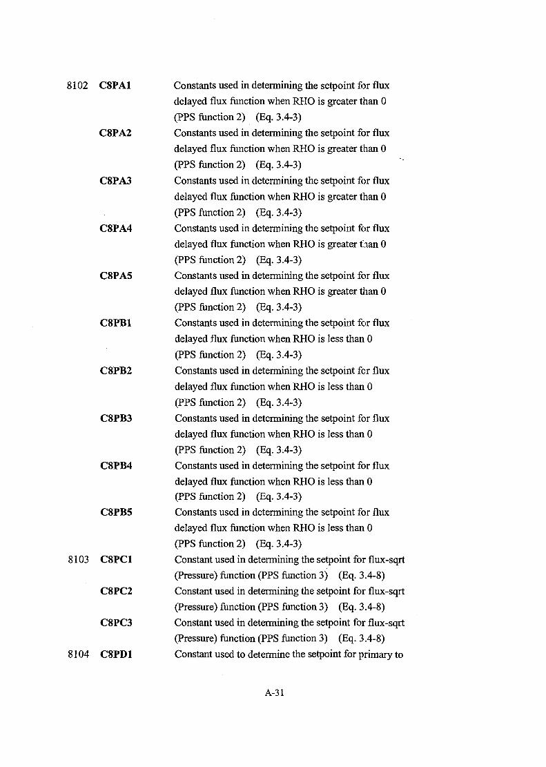
8102 C8PA1
C8PA2
C8PA3
C8PA4
C8PA5
C8PB1
C8PB2
C8PB3
C8PB4
C8PB5
8103 C8PC1
C8PC2
C8PC3
8104 C8PD1
Constants used in determining the setpoint for flux
delayed flux function when RHO is greater than 0
(PPS function 2) (Eq. 3.4-3)
Constants used in determining the setpoint for flux
delayed flux function when RHO is greater than 0
(PPS function 2) (Eq. 3.4-3)
Constants used in determining the setpoint for flux
delayed flux function when RHO is greater than 0
(PPS function 2) (Eq. 3.4-3)
Constants used in determining the setpoint for flux
delayed flux function when RHO is greater than 0
(PPS function 2) (Eq. 3.4-3)
Constants used in determining the setpoint for flux
delayed flux function when RHO is greater than 0
(PPS function 2) (Eq. 3.4-3)
Constants used in determining the setpoint for flux
delayed flux function when RHO is less than 0
(PPS function 2) (Eq. 3.4-3)
Constants used in determining the setpomt for flux
delayed flux function when RHO is less than 0
(PPS function 2) (Eq. 3.4-3)
Constants used in determining the setpoint for flux
delayed flux function when RHO is less than 0
(PPS function 2) (Eq. 3.4-3)
Constants used in determining the setpoint for flux
delayed flux function when RHO is less than 0
(PPS function 2) (Eq. 3.4-3)
Constants used in determining the setpoint for flux
delayed flux function when RHO is less than 0
(PPS function 2) (Eq. 3.4-3)
Constant used in determining the setpoint for flux-sqrt
(Pressure) function (PPS function 3) (Eq. 3.4-8)
Constant used in determining the setpoint for flux-sqrt
(Pressure) function (PPS function 3) (Eq. 3.4-8)
Constant used in determining the setpoint for flux-sqrt
(Pressure) function (PPS function 3) (Eq. 3.4-8)
Constant used to determine the setpoint for primary to
A-31

C8PD2
C8PD3
C8PD4
C8PD5
C8PD6
8201 MODIDZ8CRIN
Z8CRMX
Z8SATZ8LOCR
Z8CRUP
U8CRDN
U8CRUP
F8ROMX
intermediate speed ratio function (PPS function 4)
(Eq. 3.4-9)
Constant used to determine the setpoint for primary to
intermediate speed ratio function (PPS function 4)
(Eq. 3.4-9)
Constant used to determine the setpoint for primary to
intermediate speed ratio function (PPS function 4)
(Eq. 3.4-9)
Constant used to determine the setpoint for primary to
intermediate speed ratio function (PPS function 4)
(Eq. 3.4-9)
Constant used to determine the setpoint for primary to
intermediate speed ratio function (PPS function 4)
(Eq. 3.4-9)
Constant used to determine the setpoint for primary to
intermediate speed ratio function (PPS function 4)
(Eq. 3.4-9)
PPS/PCS module identifier*
Initial position of the primary control rods.
May vary from 0.0 (Fully inserted) to the value
assigned Z8CRMX (Fully withdrawn) (Eq. 3.4-34)
Maximum insertion limit of the primary control rods
(Eq. 3.4-34)
Primary control rod saturation position
Lower position of the rod bank before the next bank
movement begins
Upper position of the rod bank before the next bank
movement begins
Primary control rod downward velocity
(negative value) (Eq. 3.4-36)
Primary control rod upward velocity
(positive value) (Eq. 3.4-36)
Maximum reactivity of the primary control rod
banks (Eq. 3.4-34)
Note: A MODID is a three (3) digit code designed to
uniquely identify a PCS controller. Since a control rod
bank is defined with neither sub-system nor loop
[m]
[m][m]
[m]
[m]
[m/s]
[m/s]
[$]
A-32

8301 MODIDM8MOTRN8POLE
Q8FRERC8PCS
C8ACTF8HSPLR8MAX
R8ROTU8SRPM
8400 N8CSCD(I)
dependencies, digits one (1) and three (3) are by
convention always assigned a value of zero (0). The
remaining digit (2) designates the bank to wliich the
data is associated. It's value will range from one (1) to
the user defined maximum number of control rod
banks (N8CBNK) which is found on record 8001
PPS/PCS module identifier *
Motor type flag (0/1, squirrel cage/wound rotor)
Number of pairs of poles for squirrel cage type motor
(Eq. 3.4-43)
100% reference frequency of the motor-generator set [Hz]
Constants associated with the pump drive system
(Eq. 3.4-40)
Actuator constants (Eq. 3.4-44)
Pump high speed limit
Maximum resistance of the liquid rheostat actuator
(Eq. 3.4-51) [Q]
Motor resistance (Eq. 3.4-50) [Q]
Synchronous speed of the sodium pumps [rpni]
(Eq. 3.4-53)
Note: * A MODID is a three (3) digit code designed to
uniquely identify a PCS controller. Since there is only
one driver per pump and one pump per loop, the second
digit of the pump controller MODID is superfluous and is
by convention always assigned a value of zero (0).
The first digit of the MODID code is assigned on a subsystem
basis. A pump driver in a primary heat transport system is
assigned a value of one. (1) while the secondziry system
counterpart is assigned a value of two (2). The plant loop is
identified by the MODID's last digit. It's range of valid values
is one (1) through the maximum number of loops simulated
(N1LOOP).
Number of flow controller cascades associated with
each subsystem component (1=1 ,(4*N1 LOOP+3))
Note: The following cascade sequencing is assumed:
- Primary heat transport system (one entry for each loop)
- Secondary heat transport system (one entry for each loop)
A-33

8401 MODID
M8FLAG
F8GAINF8REPTC8TIMEF8ROLUF8ROLDF8DBNDX8PMC8TIMEC8FP
- Feedwater water pump (one entry for each loop)
- Feedwater valve (one entry for each loop)
- Throttle valve
- Bypass valve
- Relief valve
PPS/PCS module identifier*
Controller mode flag (0/1, automatic/manual)
(Figure 3.4-3)
Controller gain (Eq. 3.4-22)
Integral controller repetition rate
Time constants (Eq. 3.4-22)
Integral limiter (Upper limit)
Integral limiter (Lower limit)
Dead band (Fraction of 1)
Manual adjustable setpoints for controllers
Time constants
Flow controller part load profile coefficients for load
dependent set points
Note: A MODID is a three (3) digit code designed to
uniquely identify a PCS controller. The first digit
denotes the subsystem/component. It may assume values
of one (1) through eight (8) in accordance with the
following definition:
1 - Primary heat transport system
2 - Secondary heat transport system
3 - Feedwater pump
4 - Feedwater valve
5 - Throttle valve
6 - Bypass valve
7 - Relief valve
8 - Power controller
Digit two (2) identifies a cascade within a subsystem.
It is assigned a value of one(l) to a user defined
maximum. For subsystems 1 through 7, this maximum
is defined by a corresponding entry on the REORD 8400.
The maximum number of power controllers(subsystem 8)
is defined on RECORD 8001. The plant loop is
[1/s]
[s]
[s]
A-34

9001 S9LASTS9MAXAS9MINAS9SINTS9PINT(J)
S9PINT(J+1)
9002 F1EMXA
F1WMXA
F5MAXAF6MAXA
9003 F1ICDA
F6ICDA
identified by the last digit of the MODID. It's range is
zero (0) through the maximum number of loops simulated
(NILOOP). A valve of zero (0) in the third digit indicates
no loop dependency. By convention, a zero (0) is always
assigned to the third digit of power controller MODID.
Total problem simulation time
Maximum time step allowed
Minimum timestep allowed
Master clock interval at which a restart dump will occur
Master clock interval at which a system report will be
generated.
Master clock time after which the corresponding S9PINT
is no longer valid.
Note: The index J is incremented over the set of
paired points. There may be as many pairs (intervals)
as the users find necessary.
S9PINT(1) is imposed from time 0.0 to S9PINT(2).
S9PINT(3) is then used from the master clock time
S9PINT(2) to S9PINT(4). Similarly, S9PINT(5) is used
from S9PINT(4) to S9PINT(6), and so on.
It should be apparent that S9PINT(4) must be strictly
greater than S9PINT(2), and S9PINT(6) must be strictly
greater than S9PINT(4), and so on.
There is quite a bit of latitude permitted in the selection
Of print intervals, but they must be carefully chosen
(see section 7.8)
Relative accuracy acceptance limit for loop thermal
calculations
Relative accuracy acceptance limit for loop hydraulic
calculations
Relative accuracy acceptance limit for fuel calculations
Relative accuracy acceptance limit for in-vessel coolant
calculations
Relative interface condition acceptance limit for loop
hydraulic calculations
Relative interface condition acceptance limit for
in-vessel coolant calculations
[s][s]
M[s]
[s]
[s]
A-35

9004 L1ECAL
L1WCAL
L3CALL
L5CALL
L6CALL
L8CALL
9005 L1EPRT
L1WPRT
L3PRNT
L5PRNT
L6PRNT
L8PRNT
9006
9008 L9DMPZ
L9DMPI
L9DMPL
L9TBLD
Loop thermal option;
1 - module is called, 0 - module is not called
Loop hydraulic option;
1 - module is called, 0 - module is not called
Steam generator option;
1 - module is called, 0 - module is not called
Fuel option;
1 - module is called, 0 - module is not called
In-vessel option;
1 - module is called, 0 - module is not called
PCS option;
1 - module is called, 0 - module is not called
Loop thermal report option;
0 - no report, 1 - report is generated
Loop hydraulic report option;
0 - no report, 1 - report is generated
Steam generator report option;
0 - no report, 1-4 - report is generated with
correspondingly greater detail
Fuel report option;
0 - no report, 1 - report is generated
In-vessel coolant report option;
0 - no report, 1 - report is generated
PPS/PCS report option;
0 - no report, 1 - report is generated
set to 0
Dump labeled common before initialization;
1 - yes, 0 - no
Dump labeled common after initialization;
1 - yes, 0 - no
Dump labeled common after last time step;
1 - yes, 0 - no
Dump container array table information;
1 - yes, 0 - no
Note: This is currently valid only on CDC installations.
A-36

TRNREG
May be used to alter a transient proceeding from a restart at simulation time
greater than zero. Corresponds to TRNDAT RECORDS 9001 and 9005.
Rec. Variable101 S9LAST
S9MAXAS9MINAS9SINT
S9PINT(J)
S9PINT(J+1)
105 L1EPRT
L1WPRT
L3PRNT
L5PRNT
DescriptionTotal problem simulation time [s]
Maximum time step allowed [s]
Minimum time step allowed [s]
Master clock interval at which a restart dump will
occur
Master clock interval at which a system report will
be generated.
Master clock time after which the corresponding
S9PINT is no longer valid.
Note: The index J is incremented over the set of
paired points. There may be as many pairs
(intervals) as the users find necessary.
S9PINT(1) is imposed from time 0.0 to S9PINT(2).
S9PINT(3) is then used from the master clock
time S9PINT(2) to S9PINT(4). Similarly, S9PINT(5) is
used from S9PINT(4) to S9PINT(6), and so on.
It should be apparent that S9PINT(4) must be strictly
greater than S9PINT(2), and S9PINT(6) must be
strictly greater than S9PINT(4), and so on.
There is quite a bit of latitude permitted in this selection
Of print intervals, but they must be carefully chosen
(see section 7.8)
Loop thermal report option;
0 - no report, 1 - report is generated
Loop hydraulic report option;
0 - no report, 1 - report is generated
Steam generator report option;
0 - no report, 1-4 - report is generated
with correspondingly greater detail
Fuel report option;
Unit
[s]
[s]
[s]
A-37

0 - no report, 1 - report is generated
L6PRNT In-vessel coolant report option;
0 - no report, 1 - report is generated
L8PRNT PPS/PCS report option;
0 - no report, 1 - report is generated
OLDATA:
Exercise of other than default program control for the generation and
subsequent use of restart data files.
A-38
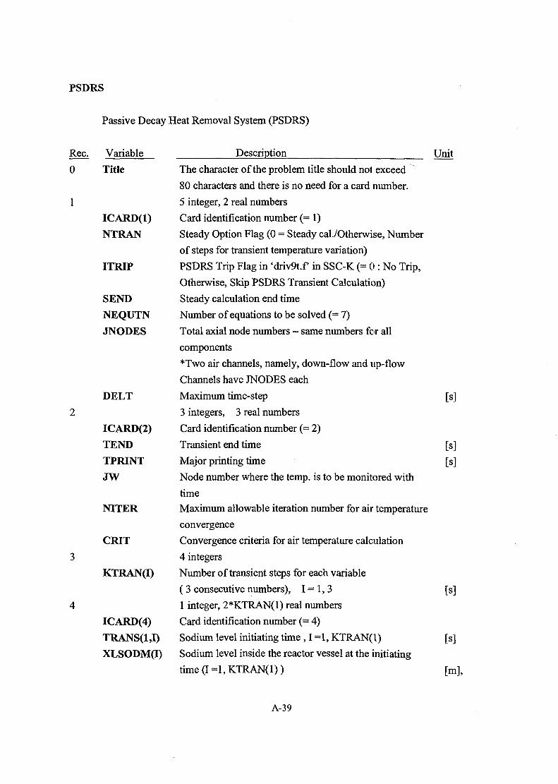
PSDRS
Passive Decay Heat Removal System (PSDRS)
Rec. Variable
0 Title
ICARD(l)
NTRAN
ITRIP
SEND
NEQUTNJNODES
DELT
ICARD(2)TENDTPRINTJW
NITER
CRIT
KTRAN(I)
ICARD(4)TRANS(1,I)
XLSODM(I)
Description UnitThe character of the problem title should not exceed
80 characters and there is no need for a card number.
5 integer, 2 real numbers
Card identification number (=1)
Steady Option Flag (0 = Steady cal./Otherwise, Number
of steps for transient temperature variation)
PSDRS Trip Flag in 'driv9t.f in SSC-K (= 0 : No Trip,
Otherwise, Skip PSDRS Transient Calculation)
Steady calculation end time
Number of equations to be solved (= 7)
Total axial node numbers - same numbers for all
components
*Two air channels, namely, down-flow and up-fiow
Channels have JNODES each
Maximum time-step [s]
3 integers, 3 real numbers
Card identification number (= 2)
Transient end time [s]
Major printing time [s]
Node number where the temp, is to be monitored with
time
Maximum allowable iteration number for air temperature
convergence
Convergence criteria for air temperature calculation
4 integers
Number of transient steps for each variable
( 3 consecutive numbers), 1=1,3 [s]
1 integer, 2*KTRAN(1) real numbers
Card identification number (= 4)
Sodium level initiating time , I =1, KTRAN(l) [s]
Sodium level inside the reactor vessel at the initiating
time(I=l,KTRAN(l)) [m],
A-39

10
1 integer, 2*KTRAN(2) real numbers
ICARD(5) Card identification number (= 5)
TRANS(24) Sodium temp, initiating time, I =1 ,.KTRAN(2)
TEMPNAQQ Sodium temp, inside the Rx vessel at the initiating time
I=1,KTRAN(2)
1 integer, 2*KTRAN(3) real numbers
ICARD(6) Card identification number (= 6)
TRANS(1,1) Cover gas initiating time, 1=1, KTRAN(3)
TEMPHE(I) Cover gas (HE) temp, inside the Rx vessel at the
initiating time, I =1, KTRAN(3)
1 integer, 6 real numbers
ICARD(7) Card identification number (= 7)
DXRV Thickness of reactor vessel
DXGV Thickness of guard vessel
DXCON Thickness of concrete wall
DHGVFI Hydraulic diameter between guard vessel and
finned shell
HRX Height of active reactor vessel
DHRX Hydraulic Diameter of the inner Rx vessel
1 integer, 6 real numbers
ICARD(8) Card identification number (= 8)
ZINLET Height of air channel inlet to the ref. position
DELZIN Length of air channel inlet
AREAIN Air channel inlet area
DHINLT Hydraulic diameter of inlet air channel
AAIR2 Down-flowing air channel area
DHADWN Hydraulic diameter of down-flowing air channel
1 integer, 6 real numbers
ICARD(9) Card identification number (= 9)
ZSTACK Height of air channel stack to the ref. position
DELZSK Length of air channel stack
ARE ASK Air flow area of stack
DHSTCK Hydraulic dia. of stack
AAIR1 Up-flowing air channel area
DHAUP Hydraulic diameter of up-flowing air channel
1 integer, 3 real numbers
ICARD(10) Card identification number (= 10)
[s]
[s]
[m]
[mj
[m]
[m]
[m]
[m]
[m]
[m]
[m2]
[m]
[m2]
[m]
[m]
[m]
[m2]
[m]
[m2]
[m]
A-40

AREAFR Turbulence friction factor
BCONST Constant to be used for boundary Reynold number
between turbulent flow and laminar flow
AREAFL Laminar friction factor
11 1 integer, 6 real numbers
ICARD(11) Card identification number (=11)
ANW01 Vessel inner heat transfer area per unit length [W/m]
AW012 Circumference between reactor vessel and
guard vessel [W/m]
AW023 Circumference between guard vessel and
inner finned shell [W/m]
AW034 Circumference between inner finned shell and
outer finned shell [W/m]
AW045 Circumference between outer finned shell and
Concrete [W/m]
AW056 Circumference of concrete wall between the positions
of TEMPW5(J) and TEMPW6 [W/m]
12 1 integer, 4 real numbers
IC ARD(12) Card identification number (= 12)
AW02A Outer circumference of guard vessel [W/m]
AW03A Inner circumference of finned shell [W/m]
AW04A Outer circumference of finned shell [W/m]
AW05A Inner circumference of concrete [W/m]
13 1 integer, 2 real numbers
ICARD(13) Card identification number (= 13)
FKORI1 Form Loss Coefficients for Orifices in the up-flowing
channel
FKORI2 Form Loss Coefficients for Orifices in the down-flowing
channel
14 1 integer, 1 real numbers
ICARD(14) Card identification number (= 14)
HCONHE Vessel inner heat transfer coef. between Helliium and
vessel wall [W/m2-°C]
15 1 integer, JNODES real numbers
ICARD(15) Card identification number (= 15)
HCV12(J) Heat transfer coef. between reactor vessel and
guard vessel, J=l, JNODES [W/m2-°C]
A-41

16
17
18
19
20
21
22
ICARD(16)
HW034
HW056
ICARD(17)
WLMASSfl)
ICARD(18)
WLSPEC(I)WLCONK(I)
ICARD(19)EPSRVEPSGVIEPSGVOEPSFSIEPSFSOEPSOW
CONCK
ICARD(20)TEMPINTEMPW6WAIRO
ICARD(21)XLSODM1TEMPNA1TEMPHE1
ICARD(22)TEMPITEMP2TEMPA
1 integer, 2 real numbers
Card identification number (= 16)
Heat transfer coef. between inner node and
outer node of divider
Heat transfer coef. between concrete and
constant heat sink
1 integer, 5 real numbers
Card identification number (= 17)
Mass per unit length for each wall
1 integer, 10 real numbers
Card identification number (= 18)
Specific heat for each wall
Thermal conductivity for each wall
1 integer, 7 real numbers
Card identification number (= 19)
Emissivity on reactor vessel wall
Emissivity on guard vessel inner wall
Emissivity on guard vessel outer wall
Emissivity on finned shell inner wall
Emissivity on finned shell outer wall
Emissivity on concrete wall
Thermal conductivity of concrete
1 integer, 4 real numbers
Card identification number (= 20)
Inlet air temperature
Constant concrete outer wall temperature
Initial user guessing air flow rate
1 integer, 2 real numbers
Card identification number (=21)
Initial sodium level in the reactor vessel
Initial sodium temp, in the reactor vessel
Initial cover gas (Helium) temp, in the reactor vessel
1 integer, JNODES real numbers
Card identification number (= 22)
Reactor vessel initial temp.
Guard vessel initial temp.
Upflow air initial temp.
[W/m2-°C]
[W/m2-°C]
[Kg/m]
[J/Kg-°C]
[W/m-°C]
[W/m-°C]
[kg/s]
[m]
A-42

TEMP3 Divider inner node initial temp. [°C]
TEMP4 Divider shell outer node initial temp. [°C]
TEMP5 Concrete inner node initial temp. [°C]
A-43


APPENDIX B Subroutines in SSC-K
The SSC-K code has a modularized structure. The code is divided into three major
sequentially disjointed processes of MAIN9R, MAIN9S, and MAIN9T as shown in Fig. B.I.
These routines are the main driver programs and are called in succession by the controller
routine. Each performs a unique set of tasks and is executed only once for any given case. It
should be noted that the modules necessary to describe the characteristics of the pool design and
reactivity models for metallic fuel were changed or added to the SSC-K code. The remainder of
the code was obtained from the SSC-L library.
The flow chart of each of the drivers, along with its associated subroutines, is shown in
Figs. B.I through B.5. Note on these figures that subroutines designated by an underline are the
changed or added ones for SSC-K. A brief description of all subroutines used in SSC-K, except
for the MINET code portion, is presented in Appendix B.
B-l
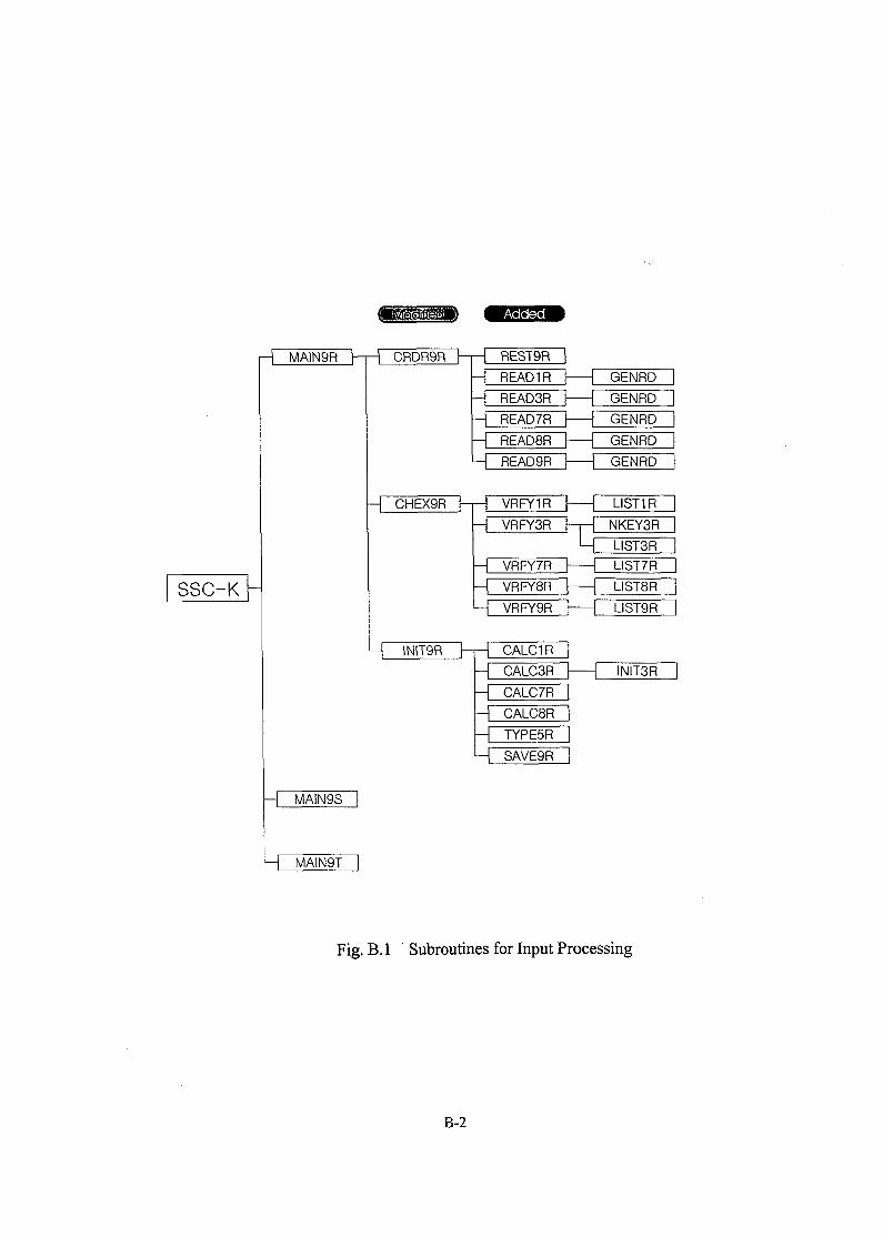
H MMN9R~
SSC-K
CRDR9R REST9R
READ1R | 1 GENRD
READ3R | 1 GENRD'
READ7R
READ8R
READ9R
IN!T9R
MAIN9S
H MAIN9T
VRFY3R
VRFY7R
VRFY8R
VRFY9R
CALC1R
CALC3R
CALC7R
CALC8R
TYPE5R
SAVE9R
GENRD
GENRD
GENRD"
H CHEX9R 1 - H VRFYTR""] 1 LIST1R
NKEY3R
LIST3R
LIST7R "
LIST8R
LIST9R
INIT3R
Fig. B.I Subroutines for Input Processing
B-2

MAIN9RCRDR9R
REST9R
READ1R
GENRDREAD3R
GENRDREAD7R
GENRDREAD8R
GENRDREAD9R
GENRDCHEX9R
VRFY1RLIST1R
VRFY3RNKEY3RLIST3R
VRFY7RLIST7R
VFRY8RLIST8R
VRFY9RLIST9R
INIT9RCALC1R
CALC3RINIT3R
CALC7R
CALC8R
TYPE5R
SAVE9R
main driver for the input initialization moduleprimary controller for the processing of initializationdata. It calls the free-format reader routinesreads a program generated file for the re-initialization of labeledcommon in the event of a restartprocesses the input for the initialization of the primary andsecondary loop modulegeneral purpose reader routineprocesses input for the initialization of the steam generator modulegeneral purpose reader routineprocesses input for the initialization of the in-vessel modulegeneral purpose reader routineprocesses input for the initialization of the plant balance routinegeneral purpose reader routineprocesses input for the initialization of the material propertyparametersgeneral purpose reader routinecalls for the verification routinesvalidates the data processed by the corresponding READ routineslists the data processed by the corresponding READ routinesvalidates the data processed by the corresponding READ routinesassists in the decoding of steam generator inputlists the data processed by the corresponding READ routinesvalidates the data processed by the corresponding READ routineslists the data processed by the corresponding READ routinesvalidates the data processed by the corresponding READ routineslists the data processed by the corresponding READ routinesvalidates the data processed by the corresponding READ routineslists the data processed by the corresponding READ routinescalls a series of intermediate data management routinesmanipulates certain primary and secondary loop input data /initializes subsequent loop structuresloads the input data into the data arraysinitializes certain steam generator constantssets slice-type dependent arrays and determines normalized axialand radial power distributioninterprets the coded iterative scheme for establishing the initial plantbalanceloads channel-dependent parameters for vise in the slice-type-dependent in-vessel modulesgenerates an ordered file for a re-initialization restart
B-3
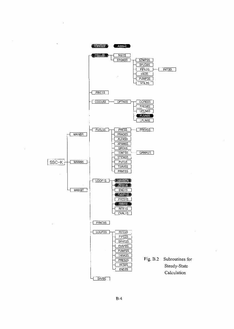
-TPINTIS
C00L6S
H MAIN9R
SSC-K MAIN9S
H MAIN9T
0PTN6S C0RE6S
PRES6S"
UPIN6S"
H LPLN6S
- I FUEL5S h - H PRE5S I 1 PREX5S
-\ FRAD5S |
H ALFA5S [
H XPAN5S |
H GR05S I
- I TEMP5S~| 1 GAMA5S
H STEM5S"
PUT5S "
TSAV5S
PRNT5S
H L00P2S" HHHH
HHHH
RITE2S
PIPE2S
SPHT2S
EVAP2S
PUMP2S
TANK2S
PRES2S
RES2S
EN02S
Fig. B.2 Subroutines for
Steady-State
CalculationH SAV9S
B-4

MAIN9S
PBAL9SIHX1S
STGN3SSTMP3SSFL03SPEPE3S
INIT3S
HX3S
PUMP3S
V0L3S
PINT1SCOOL6S
0PTN6S
C0RE6S
PRES6SUPLN6S
FLSA6SLPLN6S
FUEL5S
PRE5S
main driver for the steady-state calculations
performs the global thermal balance for the whole plantsolves the steady-state energy equations for the IHX. IHX1S andHYDR1S are the only interface between the primary andintermediate loopmain driver for the SG calculationsdetermines the sodium inlet temperaturedetermines the sodium flow rate per tubecomputes the pressure at the exit of a pipeloads initial guesses for steam pressures, mass flow rates, enthalpiesand heat transfer rates. Values for pressure and mass are user-input.Initial enthalpies and heat transfer rates are zeroed, as ENET3S iscalled soon after INIT3S.performs the heat exchanger model calculations. It determines thepressure drop in the inlet plenum of the heat exchanger, calls theroutines which determines the enthalpy and pressure distributions inthe heat transfer tube, and calculates the pressure drop in the outletplenum of the heat exchanger. It determines the location of theDNB point and adjusts the total heat transfer area to producespecified outlet conditions.computes the pump outlet pressure at rated pump speed or the pumpspeed if the pump outlet pressure is specifiedcalculates the mixed mean enthalpy in a volume based on the liquidlevel and the pressure specified in the volumeinterfaces the in-vessel and primary loop pressuresdriver module for in-vessel coolant calculationscomputes the steady-state channel flow rate distribution or pressureloss coefficientscore coolant: It calculates axial temp., enthalpy gradients, frictionfactors, heat transfer coefficients and pressures each node in eachchanneldetermines the nodal pressures in each reactor coolant channelcoolant module: calculates upper plenum temp, exit quality, outlet,and top of core pressures and finds pressure loss factors for eachchannelcalculates pressure equalization loss coefficient at top of assemblylower plenum module: initializes values of temperature, enthalpy,and pressure for the first axial nodal interface of each channel. Itcalculates pressures at the bottom of the coredriver module for fuel heat conduction calculations. It treats a fuelslice as the basic computational element, calls all major fuelcomputational modules, and controls convergenceperforms the initialization for FUEL5S bjf obtaining data computedby other modules. Among others, it sets the proper rod nodal
B-5
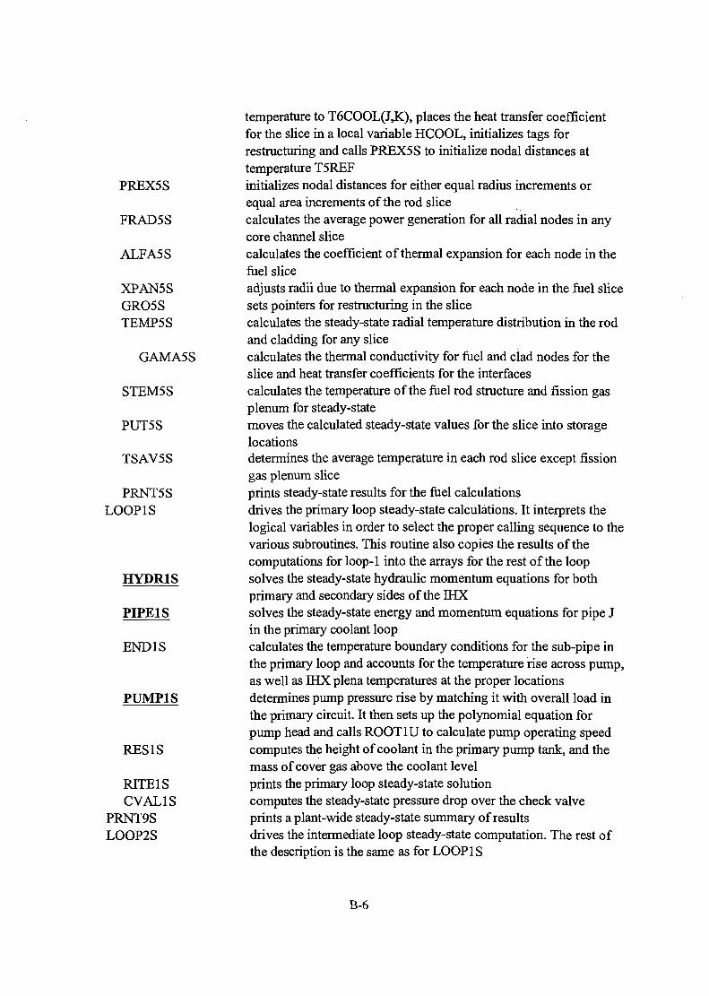
PREX5S
FRAD5S
ALFA5S
XPAN5SGR05S
TEMP5S
GAMA5S
STEM5S
PUT5S
TSAV5S
PRNT5SLOOP IS
HYDR1S
PIPE1S
END1S
PUMP1S
RES1S
RITE1SCVAL1S
PRNT9SLOOP2S
temperature to T6COOL(J,K), places the heat transfer coefficientfor the slice in a local variable HCOOL, initializes tags forrestructuring and calls PREX5S to initialize nodal distances attemperature T5REFinitializes nodal distances for either equal radius increments orequal area increments of the rod slicecalculates the average power generation for all radial nodes in anycore channel slicecalculates the coefficient of thermal expansion for each node in thefuel sliceadjusts radii due to thermal expansion for each node in the fuel slicesets pointers for restructuring in the slicecalculates the steady-state radial temperature distribution in the rodand cladding for any slicecalculates the thermal conductivity for fuel and clad nodes for theslice and heat transfer coefficients for the interfacescalculates the temperature of the fuel rod structure and fission gasplenum for steady-statemoves the calculated steady-state values for the slice into storagelocationsdetermines the average temperature in each rod slice except fissiongas plenum sliceprints steady-state results for the fuel calculationsdrives the primary loop steady-state calculations. It interprets thelogical variables in order to select the proper calling sequence to thevarious subroutines. This routine also copies the results of thecomputations for loop-1 into the arrays for the rest of the loopsolves the steady-state hydraulic momentum equations for bothprimary and secondary sides of the IHXsolves the steady-state energy and momentum equations for pipe Jin the primary coolant loopcalculates the temperature boundary conditions for the sub-pipe inthe primary loop and accounts for the temperature rise across pump,as well as IHX plena temperatures at the proper locationsdetermines pump pressure rise by matching it with overall load inthe primary circuit. It then sets up the polynomial equation forpump head and calls R00T1U to calculate pump operating speedcomputes the height of coolant in the primary pump tank, and themass of cover gas above the coolant levelprints the primary loop steady-state solutioncomputes the steady-state pressure drop over the check valveprints a plant-wide steady-state summary of resultsdrives the intermediate loop steady-state computation. The rest ofthe description is the same as for LOOP IS
B-6

RITE2SPIPE2S
SPHT2S
EVAP2S
PUMP2S
TANK2S
PRES2S
RES2S
END2S
SAV9S
prints the secondary loop steady-state solutionsolves the steady-state energy and momentum equations for pipe Jin the intermediate coolant loopcalculates the pressure drop or loss coefficient on the shell side ofthe superheatercalculates the pressure drop or loss coefficient on the shell side ofthe evaporatordetermines pump pressure rise by matching it with overall load inthe intermediate circuitcomputes the pressure in the loop at the location of the surge tank,and further, calculates the mass of gas in the surge tankdetermines the pressure at pipe end points around the intermediateloopcomputes the height of coolant in the intermediate pump tank, andthe mass of cover gas above the coolant levelsets the inlet temperature and mass flow rate boundary conditionsfor pipe J+l in the intermediate coolant loopcreates an ordered file containing information necessary to re-initialize all common blocks to computed steady-state values
B-7

Fig. B.3 Subroutines for
Transient
Calculation
B-8

I DR1V1T hpf~bOPP5T [
V0ID5T I
GR0W5T |
- ( FLOW2T
H PRES2T'
H ST0R1T~1
H IHX1T |
PIPE2T |
- I BREK2T | 1 VJ1T
H PLOS2T |
H PUMP2T
FUNC2T
BREK1T [ 1 VJ1T
Fig. B.3 Subroutines for Transient Calculation (Continued)
B-9

MAIN9T
CRDR9T
INIT9T
TBLDMPCNTDMPCOMDMPINIT6T
INIT1T
DEFN1T
XI1T
EQIV1T
INIT2T
INTG1T
PRET1T
INIT5T
INIT8T
COUR9TREAD9T
GENRD
VRFY9T
LIST9T
INIT3T
INTF3T
DRTV9T
DRTV1T
REAC5T
overall driver routine for the transient calculations
intermediate controller for the transient initialization routines
lists global container allocations
list all global locations in the container
initiates variables used by the in-vessel coolant hydraulics modules
sets variables needed for the first call to the primary loop hydraulic
integration scheme
defines pipe flow rates, and input and output pump flow rates for
primary loop
equivalences the names of primary loop variables and their time
intervals in terms of names in the integrating subroutine
sets variables needed for the first call to the secondary loop
hydraulic integrating routine
advances the hydraulic equations using the predictor-corrector
method of the Adams type
initializes the primary and secondary loop variables for the thermal
calculations
initializes variables used in the fuel and reactivity calculations
initializes values used in the PPS/PCS subroutines
calculates Courant condition for all channels
reads free-format card-image input for the initialization of transient
parameters
general purpose reader routine
validates the data processed by the READ9T routine against the
criteria established in the data dictionary
lists the data processed by READ9T
initializes transient variables used by the steam generator modules
interfaces the required boundary conditions between all
intermediate sodium loops and all steam generator heat exchanger
driver routine for the transient calculations. It also handles the
overall time step control
driver for heat transport system transient hydraulics
initiates calls to other modules to obtain the various applied and
B-10
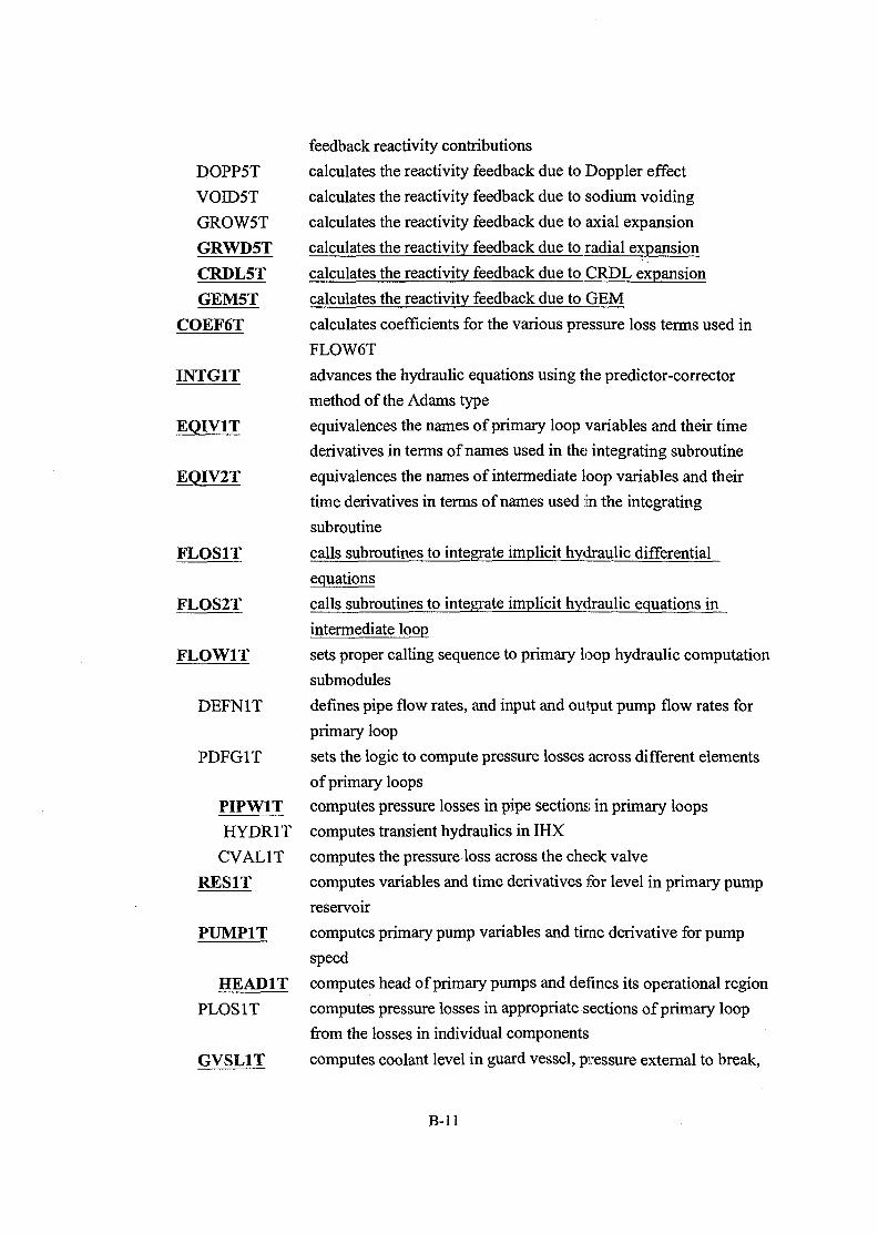
D0PP5T
V0ID5T
GR0W5T
GRWD5TCRDL5TGEM5T
COEF6T
INTG1T
EQIV1T
EQIV2T
FLOS1T
FLOS2T
FLOW1T
DEFN1T
PDFG1T
PIPW1THYDR1T
CVAL1T
RESIT
PUMP1T
HEAP1T
PLOS1T
GVSL1T
feedback reactivity contributions
calculates the reactivity feedback due to Doppler effect
calculates the reactivity feedback due to sodium voiding
calculates the reactivity feedback due to axial expansion
calculates the reactivity feedback due to radial expansion
calculates the reactivity feedback due to CRDL expansion
calculates the reactivity feedback due to GEM
calculates coefficients for the various pressure loss terms used in
FL0W6T
advances the hydraulic equations using the predictor-corrector
method of the Adams type
equivalences the names of primary loop variables and their time
derivatives in terms of names used in the integrating subroutine
equivalences the names of intermediate loop variables and their
time derivatives in terms of names used in the integrating
subroutine
calls subroutines to integrate implicit hydraulic differential
equations
calls subroutines to integrate implicit hydraulic equations in
intermediate loop
sets proper calling sequence to primary loop hydraulic computation
submodules
defines pipe flow rates, and input and output pump flow rates for
primary loop
sets the logic to compute pressure losses across different elements
of primary loops
computes pressure losses in pipe sections; in primary loops
computes transient hydraulics in IHX
computes the pressure loss across the check valve
computes variables and time derivatives for level in primary pump
reservoir
computes primary pump variables and time derivative for pump
speed
computes head of primary pumps and defines its operational region
computes pressure losses in appropriate sections of primary loop
from the losses in individual components
computes coolant level in guard vessel, pressure external to break,
B-ll

VESL1T
BREK1T
VJ1T
PRUP6T
UPLN6T •
PRUP6T
UPLS6T
FL0W6T
PRES1T
FUNC1T
EQIV1T
FLOW2T
FUNC2T
PRJES2T
BREK2T
VJ1T
PL0S2T
PUMP2T
T0RK2T
HEAD2T
and time derivative for accumulated volume of coolant in the guard
vessel
calculates certain algebraic relationships at the vessel-loop(s)
interface(s) and within the vessel which are used in the hydraulic
computations
computes pressures at eventual break in primary loop
determines velocity of jet out of a pipe break
calculates the vessel outlet pressure and core top pressure for the
one-dimensional two zone upper plenum model
one-dimensional two zone upper plenum model
calculates the vessel outlet pressure and core top pressure for the
one-dimensional two zone upper plenum model
updates the time derivatives for sodium level, sodium temperatures
in two mixing zones, cover gas temperature, and temperature of the
inner structure, thermal liner and vessel
simulates the flow redistribution model. It calculates the mass flow
rate in each channel and bypass channel
sets inlet and outlet pressures of uniform mass flow rate sections in
primary loops
calculate the time derivatives of differential equations for primary
loop hydraulics
equivalences the names of primary loop variables and their time
derivatives in terms of names used in the integrating subroutine
sets proper calling sequence to intermediate loop hydraulic
computation submodules
calculate the time derivatives of differential equations for
intermediate loop hydraulics
sets inlet and outlet pressures of uniform mass flow rate sections in
intermediate loops
computes pressures at eventual break in intermediate loop
determines velocity of jet out of a pipe break
computes pressure losses in appropriate sections of intermediate
loop from the losses in individual components
computes intermediate pump variables and time derivatives for
pump speed
computes hydraulic and friction torques for intermediate pumps
computes head of intermediate pumps and defines its operational
B-12

RES2T
TANK2T
PDFG2T
EVAP2T
SPHT2T
HYDR1T
PIPW2T
DEFN2T
EQIV2T
ST0R1T
IHX1T
PIPE2T
POW5T
PRMT5T
STGN3T
UP2D6T
IMPX1T
LOOP1TPIPE1T
IHX1TEND1T
LOOP2T
IHX1T
PIPE2T
END2T
region
computes variables and time derivatives for level in intermediate
pump reservoir
computes pressures and time derivatives for level in surge tank
sets the logic to compute pressure losses across different elements
of intermediate loops
computes pressure loss across the shell side of evaporator
computes pressure loss across the shell side of superheater
computes transient hydraulics in IHX
computes pressure losses in pipe sections in intermediate loops
defines pipe flow rates, and input and output pump flow rate for
intermediate loop
equivalences the names of intermediate loop variables and their
time derivatives in etrms of names used in the integrating
subroutine
stores the intermediate updated values of flow rate
solves transient energy equations in the IHX
solves transient energy equations in the intermediate loop piping
serves as the driver for the rod transient fission power generation
calculations
handles the advancement in time of the fission power generation
main driver for the steam generator calculation. It calls routines
which computes accumulator conditions, backsubstitutes
accumulator conditions to advance flow sequence variables, and
determines the maximum change in water side variables during this
step2D upper plenum model
main driver for transient thermal calculations in primary loop
solves transient energy equations in the primary loop piping
solves transient energy equations in the IHX
sets transient thermal boundary conditions from one pipe to the next
in primary loop
main driver for transient thermal computations in intermediate loop
solves transient energy equations in the IHX
solves transient energy equations in the intermediate loop piping
sets transient thermal boundary conditions from one pipe to the next
B-13

PPCS8T
INT8T
SENS8T
SGEN8T
PPS8T
PC0N8T
APPL8T
FC0N8T
STGN8T
SCUT9T
INTF9T
FUEL5T
P0W6T
PRE5T
PR0P5T
XPAN5T
intermediate loop
main driver for the PPS/PCS transient calculations
interfaces the PPS/PCS modules to the rest of SSC by fetching the
actual values of the desired process variables for cascade selection
for reactor power control and normalizing them against their
respective 100% steady-state values. It also calls other subroutines
to do similar calculations for PPS, flow controllers and the steam
generator controllers
takes the actual sensed values from the controller cascades and
compensates them for the inherent time lags imposed by the
measuring devices
calculates the load-dependent setpoints as governed by the
supervisory controller, using the user specified second-order
polynomial coefficients
subdriver routine for the plant protection system
simulates the reactor power control and the control rod drive
mechanism. It also calculates the reactivity worth of the reactor
control rods
calculates the scram reactivity worth of the primary and/or
secondary control rods utilizing the user supplied polynomial
coefficients for rod position as a function of time after reactor scram
simulates the sodium flow-speed control and the pump drive
mechanism
subdriver for steam generator controller routines
controls timestep after scram
checks the adequacy of all extrapolated interface conditions
driver for the fuel rod and structure calculations. By calling series of
modules in succession; it calculates, quantities such as temperature
and radii of the fuel, cladding, and structure nodes
calculates power to coolant for use in COOL6T
transfers the temperature from storage arrays into local scratch
arrays for the particular slice in question, at the start of each time-
step
calculates all properties for the fuel (rod) heat conduction
calculations
recalculates the radii of the fuel and cladding, necessary because of
the thermal expansion of the radial nodes. Two methods are
B-14

GAMA5T
FRAD5T
SGMA5T
B0IL6T
C0EF5T
S0LV5T
PUT5T
TSAV5T
PR0P6T
INTR6TPREA6TGEOM6TC0EF6T
QCAC6TINTA6T
TWIS6TC00L6T
employed in calculating radii, equal areat increment, and equal radii
increment calculating radii; equal area increment, and equal radii
increment
calculate the thermal conductivity and emissivity for fuel and clad
nodes and also computes the heat transfer coefficient for gaseous
mixtures in the gap
calculates average power for all radial nodes in any rod slice. It also
calculates the power generation multiplier to be used later in
calculating the transient volumetric power generation
calculates the volumetric heat source for the fuel (rod) nodes, clad,
coolant and structure in an axial slice
calculates liquid and bubble temperature in upper and lower slugs
calculates appropriate coefficients for the transient temperature
calculations of fuel rod
solves the fuel (rod) matrix equation using Gaussian elimination
with fuel pivoting
at the time this module is invoked, all foimal calculations of the fuel
and clad and structure have been completed for that timestep and for
the given axial node. This module then move all temperatures and
radii so far calculated from local scratch variables into storage
arrays for subsequent timesteps
calculates certain fuel slice dependent quantities required in
GR0W5T, DOPP5T, and V0ID5T
calculates all properties used in the in-vessel coolant energy and
fluid dynamics subroutines
main driver for interassembly heat transfercalculates channel flow area
calculates coefficients for the various pressure loss terms used in
FL0W6T
calculates interassembly heat transfer
calculates interassembly heat transfer
calculates interassembly heat transfer
driver for the transient coolant calculations. It provides initial
conditions; determines step size; and then employs several
submodules to calculate temperature, pressure, enthalpy, and mass
flow rate of the coolant in all axial nodes of all channels. It then
B-15

LPLN6T
PIPE2T
PSDRS
RUNGEK
EQUTNS
COEFEQ
COEFIC
TEMPAR
FLWAIR
PSY PROP
SAV9T
PRNT9T
stores values for fuel calculations
performs transient lower plenum calculations. It extrapolates
boundary conditions. It determines its procedure by calculating
coolant and metal temperature and pressures at the bottom of the
core
solves transient energy equations in the intermediate loop piping
PSDRS «1H
n
creates an ordered file containing information necessary to re-
initialize all common blocks to a given master clock solution
main printing routine for the transient
B-16

- I FSEG3T \-r\ HX3T
Fig. B.4 Subroutines for Steam Generator (MINET Portion)
B-17

STGN3T
IKFS3T
PL0P3T
PSFW3T
FEED3T
PSTB3T
WSTE3T
PSTB3T
FSEG3T
HX3T
DPFG3TDPAC3T
FRIC3T
TPMP3T
DPFT3T
WSTE3T
SFLC3T
STMP3T
ERR3T
IKF3T
PL0P3T
PSFW3T
FEED3T
PSTB3T
WSTE3T
INFS3T
main driver for the steam generator calculation. It calls routines
which computes accumulator conditions, backsubstitutes
accumulator conditions to advance flow sequence variables, and
determines the maximum change in water side variables during this
step
determines pointers for all arrays needed in the flow segment
calculations
determines reference pressure for a flow segment
determines reference pressure for a flow segment
determines reference coefficients for feedwater flow rate
determines turbine inlet pressure
determines water properties as function of enthalpy and pressure
determines turbine inlet pressure
main driver for flow segment calculations
determines coefficients for energy and flow equation for water side
of heat exchanger and advances sodium temperature
determines coefficients of total flow resistance in control volume
determines the coefficients of momentum flux pressure loss in
control volume
determines friction factor as function of Reynolds number and
surface roughness
determines two-phase friction multiplier on the water/steam side of
the steam generator
determines coefficients of pressure drop in a fitting using form loss
coefficient
determines water properties as function of enthalpy and pressure
determines sodium temperature at heat exchanger inlet from
boundary conditions
writes error message
determines reference pressure for a flow segment
determines reference pressure for a flow segment
determines reference coefficients for feedwater flow rate
determines turbine inlet pressure
determines water properties as function of enthalpy and pressure
B-18

WSTE3T
FEED3T
PSTB3T
PUMP3T
WSTE3T
PIPE3T
DPFG3T
DPAC3T
FRIC3T
TPMP3T
WSTE3T
DPFT3T
TMS3T
TUBE3T
FUNC2T
PRES2T
BREK2T
PL0S2T
HWFB3T
ERR3T
HWFC3T
HWNB3T
HWSC3T
PUMP2T
PRES2T
determines water properties as function of enthalpy and pressure
determines reference coefficients for feedwater flow rate
determines turbine inlet pressure
determines coefficients for energy and flow equations for a pump
determines water properties as function of enthalpy and pressure
determines coefficients for energy and flow equations for a pipe
determines coefficients of total flow resistance in control volume
determines the coefficients of momentum flux pressure loss in
control volume
determines friction factor as function of Reynolds number and
surface roughness
determines two-phase friction multiplier on the water/steam side of
the steam generator
determines water properties as function of enthalpy and pressure
determines coefficients of pressure drop in a fitting using form loss
coefficient
calculates surface heat fluxes and tube wall temperatures in heat
exchanger
calculates the time derivatives of differential equations for
intermediate loop hydraulics
sets inlet and outlet pressures of uniform mass flow rate sections in
intermediate loops
computes pressures at eventual break in intermediate loop
computes pressure losses in appropriate sections of intermediate
loop from the losses in individual components
determines heat transfer coefficient in film boiling
writes error message
determines heat transfer coefficient in forced convection to liquid
determines heat transfer coefficient in nucleate boiling of subcooled
or saturated water
determines heat transfer coefficient in forced convection to super-
heated steam
computes intermediate pump variables arid time derivative for pump
speed
sets inlet and outlet pressures of uniform mass flow rate sections in
intermediate loops
B-19

PSFW3T determines reference pressure for a flow segment
FEED3T determines reference coefficients for feedwater flow rate
PSTB3T determines turbine inlet pressure
TANK2T computes pressures and time derivative for level in surge tank
HNAF3T computes sodium side surface heat transfer coefficient
ACCM3T calculates coefficients for accumulator, eliminates flow segment
terms for accumulator equations, and advances the accumulator
variables
PSFW3T determines reference pressure for a flow segment
PSTB3T determines turbine inlet pressure
B-20

Fig. B.5 All Subroutines Employed into SSC-K
B-21
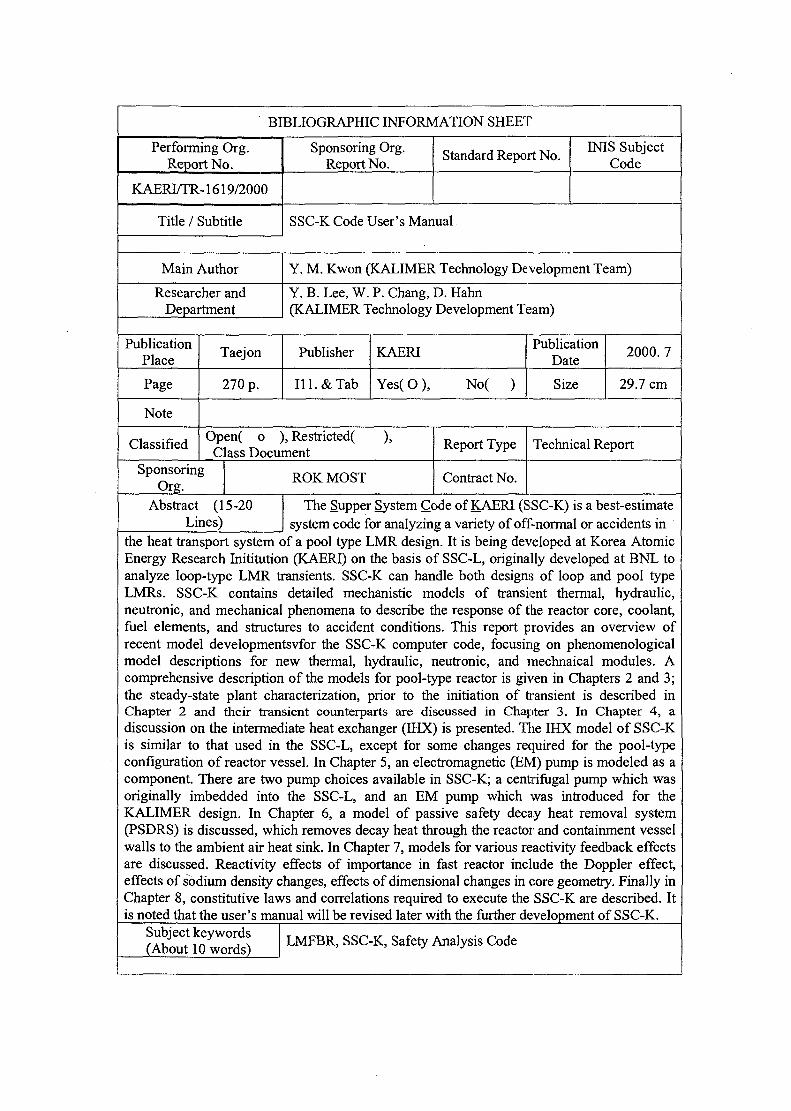
BIBLIOGRAPHIC INFORMATION SHEET
Performing Org.Report No.
Sponsoring Org.Report No.
Standard Report No. INIS SubjectCode
KAERLTR-1619/2000
Title / Subtitle SSC-K Code User's Manual
Main Author Y. M. Kwon (KALIMER Technology Development Team)
Researcher andDepartment
Y. B. Lee, W. P. Chang, D. Hahn(KALIMER Technology Development Team)
PublicationPlace
Taejon Publisher KAERI PublicationDate
2000. 7
Page 270 p. 111. & Tab Yes( O No( Size 29.7 cm
Note
Classified Open( o ), Restricted(Class Document
Report Type Technical Report
Sponsoring ROK MOST Contract No.
Abstract (15-20Lines)
The Supper System Code of KAERI (SSC-K) is a best-estimatesystem code for analyzing a variety of off-normal or accidents in
the heat transport system of a pool type LMR design. It is being developed at Korea AtomicEnergy Research Inititution (KAERI) on the basis of SSC-L, originally developed at BNL toanalyze loop-type LMR transients. SSC-K can handle both designs of loop and pool typeLMRs. SSC-K contains detailed mechanistic models of transient thermal, hydraulic,neutronic, and mechanical phenomena to describe the response of the reactor core, coolant,fuel elements, and structures to accident conditions. This report provides an overview ofrecent model developmentsvfor the SSC-K computer code, focusing on phenomenologicalmodel descriptions for new thermal, hydraulic, neutronic, and mechnaical modules. Acomprehensive description of the models for pool-type reactor is given in Chapters 2 and 3;the steady-state plant characterization, prior to the initiation of transient is described inChapter 2 and their transient counterparts are discussed in Chapiter 3. In Chapter 4, adiscussion on the intermediate heat exchanger (IHX) is presented. The IHX model of SSC-Kis similar to that used in the SSC-L, except for some changes required for the pool-typeconfiguration of reactor vessel. In Chapter 5, an electromagnetic (EM) pump is modeled as acomponent. There are two pump choices available in SSC-K; a centrifugal pump which wasoriginally imbedded into the SSC-L, and an EM pump which was introduced for theKALIMER design. In Chapter 6, a model of passive safety decay heat removal system(PSDRS) is discussed, which removes decay heat through the reactor and containment vesselwalls to the ambient air heat sink. In Chapter 7, models for various reactivity feedback effectsare discussed. Reactivity effects of importance in fast reactor include the Doppler effect,effects of sodium density changes, effects of dimensional changes in core geometry. Finally inChapter 8, constitutive laws and correlations required to execute the SSC-K are described. Itis noted that the user's manual will be revised later with the further development of SSC-K.
Subject keywords(About 10 words)
LMFBR, SSC-K, Safety Analysis Code

KAERFTR-1619/2000
^ 1 / ^Ml
1 °1 1
^ J L A H V
wl ^ '-A ^~
270 p.
^ J i °o> ^
99C-TC ^ I A V S 1 2 AV-S-y
a^jiA^j: INIS^2H
^ ^ ^ (KALIMER 71 #7fl^;^)
^ 7 1 ^
] (KALIMER ;
5a^(o>, a*( >
7l#7fl
^ ^
3. 7l
2000.7
29.7 cm
^•7fl( o ) tll^«l( ),
&\ ?- °i EJ-7] ji}- j7l^l-7i^-Wi
71 # .S.JLA-1
(15-20 (KAERI)fe Poo l^
KALIMER S]H<?1 SSC-K (Supper System Code of KAERI)!- 7fl
KALIMER
7-1^
. SSC-K ^ ^- BNLSSC-L ^ 7 l ^ o . 5 . «
^7fl SSC-K. SSC-K fe
SI4. fe- SSC-K
SI 4.
IHX S f ft4 . 5 - fe-
KALIMER
SSC-L 3 E £ ]^:7l (IHX) 2.
^ - ^ , SSC-K fe- 7 l ^7]-
^^>4. 6 HlfePSDRS 7 -oflfe- £#51
SSC-KSSC-K SHS] ^ 1 ^
SSC-K 1-SSC-K 3 ^ f e % ^ KALIMER
(10LMFBR, SSC-K, Safety Analysis Code


![CPT100-C - Fund[1]. Canopy SP Rev.O](https://img.dokumen.tips/doc/110x75/544ee6aab1af9f27638b523e/cpt100-c-fund1-canopy-sp-revo.jpg)