Squash Sport Analytics & Image Processing

Dan Judddjudd@seas.upenn.edu

Rebecca Wurewu@seas.upenn.edu

Dr. Camillo Jose Taylorcjtaylor@cis.upenn.edu

Spring 2014

1 INTRODUCTION

Squash is a racquet sport played in a similar style room as racquetball. In a squash match there are 2players that alternate hitting a small, black, rubber ball. A complete match is played as best of 5 games,where each game is played to 11 points. Points are scored when a player fails to return a shot made bythe opponent.1

The sport of squash is played in over 190 countries by millions of people all over the world.2 Yet tothis day, no one has taken a truly analytical approach to the sport. Data analytics has recently been apopular topic of conversation in sports, with analytical systems already in place for popular sports likebasketball and baseball.3

Jack Wyant, the head coach of the Penn Varsity Squash team, feels strongly about the need andvalue of a sports analytical system for squash. Dan Judd personally identifies with this need as well, asa former top 20 junior and also a starter on the Penn Varsity Squash team. An analytical system forsquash would directly benefit squash players by analyzing their game performance and revealing possibleareas of improvement.

Under the guidance of our advisor Dr. Camillo Jose Taylor, an A-level squash player, our projectteam has made the first efforts towards meeting this need by developing computer programs to read invideo footage of squash games, perform automatic detection and motion-based tracking of the movingplayers, and output useful data analysis for squash players. Our project undertakes the technical, behind-the-scenes analysis and lays the foundation work for a consumer end-user product to be developed in thenear future.

2 PROJECT OVERVIEW

The project is comprised of two main parts that each produces its own set of output:

1. Motion-based multiple object tracking

2. Coordinate-based data analysis

1”Rules of Squash.” US Squash. http://www.ussquash.com/officiate/online-rules/2”Squash Sport Info.” Squash Source. http://www.squashsource.com/squash-sport/3”Conference Agenda.” MIT Sloan Sports Analytics Conference. http://www.sloansportsconference.com/?page id=13335

1

2.1 Motion-Based Multiple Object Tracking

The problem of motion-based multiple object tracking can be further broken down into the followingsubproblems:

• Detecting the moving objects (2 players, 1 ball) in each video frame

• Associating the detections to the same corresponding object over time

To detect the moving objects, we start by using a background subtraction function in MATLAB toisolate the moving pixels from the stationary pixels. The resulting “mask” still contains some degreeof noise and requires further refinement, so morphological operations are used to eliminate any straypixels. To differentiate separate objects, we use MATLAB’s “blob analysis” to detect distinct groups ofconnected pixels.

To associate detections to the same object from frame to frame, we assign a detection to a corre-sponding “track” that is continually updated in each frame. Tracks are stored within an array and maybe created or deleted depending on whether there are new, unassigned detections, or detections thathave been repeatedly unassigned past a specified threshold. Assignments of detections to tracks aremade using a Kalman filter, which estimates the motion of each track and determines the likelihood fora detection to be assigned to a track. Maintaining these tracks allows us to derive the (x, y) coordinatesof the two squash players and create an output .csv file containing a list of these coordinates over theduration of the video.

2.2 Coordinate-Based Data Analysis

Given the .csv file of (x, y) coordinates, we have implemented two forms of data analysis to return sportsanalytics for the squash players:

• Movement analysis

• Creating a heat map

For the movement analysis, we first output the current location on the squash court in real-worldcoordinates using the ”T” intersection of the court lines as the origin. Then we provide statistics on howfar each squash player is moving by calculating the distance between every pair of coordinates in thefile using the distance formula:

√(x2 − x1)2 + (y2 − y1)2. We also provide statistics on how fast each

squash player is moving by calculating the speed using the formula: s = D/t, where D refers to thedistance and t = 1 frame / 120fps ≈ 0.0083 seconds.4

In addition to the above metrics, it is possible to calculate the direction in which the player ismoving by using the trigonometric formula: θ = tan−1( y2−y1

x2−x1) where θ refers to the angle of the player’s

movement relative to the polar coordinate axes. An output .csv file is created containing the results ofthe movement analysis spanning the duration of the video.

For creating a heat map, we use an image of the background of the squash court as a backdrop andthen draw points onto the court representing each player’s location for every frame in the video. Overtime, there will be clusters of points that build up on the screen and reveal where each player tends tostand and what movements each player likes to make, so they can evaluate their overall movements andupdate their strategy accordingly.

This form of analysis is similar to examining the video footage itself, which is currently the dominantform of instruction used by coaches. However, the heat map carries the additional benefit of seeing thehistory of the player’s movement. This heat map image is another one of the outputs from the dataanalysis.

4The GoPro camera used to capture footage is set to 120 frames/second.

2

2.3 Summary of Obstacles/Challenges

Some problems have been trickier than others to solve due to unforeseen challenges stemming from thecolor of the players’ clothing and the high speed of the ball.

Since the color of some of the squash players’ clothing would at times blend into the background colorof the squash court walls and floor, the blob analysis tool would identify one player as multiple separateobjects rather than one cohesive object. In this case, the challenge is to recognize which objects shouldbe combined and to ensure that these updated associations are preserved in the tracking system fromframe to frame.

The high speed of the ball has also been an issue because the ball would sometimes outright disappearfor several frames after being hit by a racquet before reappearing again as a rounded blur rather than aperfectly round object. So not only is the ball entirely missing at times, but it also does not maintaina constant round shape throughout the video. Both of these issues make it very difficult to detect andtrack the ball.

The solutions we have reached for these particular challenges will be explained in more depth in thefollowing sections.

3 EQUIPMENT/SETUP

Determining the appropriate camera settings to use, the best point of view to shoot from, and the correctMATLAB functionality to apply has led to an initial trial-and-error period resulting in many failed testprograms and numerous trips to the squash courts to tape new footage. The decisions made during thatperiod are elaborated in this section.

3.1 GoPro Camera

The camera used to capture video footage of squash games is a GoPro HERO3+ Black Edition Cam-era, which comes outfitted with a wide-angle lens. It has several options for setting the number offrames/second (15fps, 30fps, 60fps, 120fps, or 240fps) along with the corresponding image resolution(4000p, 2700p, 1080p, 720p, or WVGA).5 There is a tradeoff between quantity and quality dependingon the setting:6

• A higher number of frames/second and a corresponding lower resolution results in a larger quantitybut a lower quality of frames. The benefit of having a high number of frames/second is a morecontinuous view of the objects’ motion, but the downside is a greater difficulty in accuratelydetecting objects because of the lower quality of the image.

• On the other hand, a lower number of frames/second and a corresponding higher resolution re-sults in a smaller quantity but higher quality of frames. The benefit of having a low number offrames/second is having greater accuracy in detecting objects, but the downside is a choppier viewof the objects’ motion and difficulty in assigning detections to tracks due to the fewer number offrames.

To start, we set the camera to 240 frames/second at WVGA resolution. After inputting the videointo a test program, we realized the number of frames/second was too high because the program wasprocessing the video at a halting pace and taking far too long to run. The resolution was also too low,given that we could not even see the ball in the video.

Next, we tried 60 frames/second at 1080p resolution, which solved the problem of seeing the ball butleft large gaps in between frames so that objects appeared to jump from one location to another ratherthan moving in a visibly continuous manner.

5”HERO3+ Black Edition Technical Specs.” GoPro. http://gopro.com/cameras/hd-hero3-black-edition#technical-specs6Handa, Ankur et. al. ”Real-Time Camera Tracking: When is High Frame-Rate Best?” Imperial College London.

https://www.doc.ic.ac.uk/˜ ajd/Publications/handa etal eccv2012.pdf

3

Finally, we tried 120 frames/second at 720p resolution and have found this setting to be a goodcompromise between the frame rate and quality of image. The ball is visible most of the time and thereare enough frames to track the objects consistently from frame to frame. This is the setting we haveused to capture the final set of video footage.

3.2 Point of View

In order to simplify the analysis, we have decided to capture video footage in the form of a two-dimensional flat plane rather than a three-dimensional point of view at the recommendation of Dr.Taylor. To accomplish this objective, we have the option of capturing video footage from either behindthe court at the ground level or above the court looking downwards. There are various pros and cons ofeither viewpoint:

• From behind the court, the main pro is that the entire back wall fits comfortably within the camera’sviewfinder without including unrelated objects from outside the court boundaries. However, thereare also major cons to contend with, the primary one being that the players would sometimesoverlap and make it difficult to differentiate one player from the other. Additional problems includeshaky footage when the ball hits the glass wall and poor video quality due to smudges on the glasswall itself.

• From above the court, overlapping players are no longer a problem and there are no visual ob-structions blocking the camera. But there are still cons that need to be managed since the courtfloor has more square footage to fit into the viewfinder than the court wall. To adjust, we haveused a very tall tripod to capture a view of the entire floor. The side effect of this point of view isthe inclusion of more unrelated objects from outside the court such as the bleachers and the outerwalkways. The image distortion created by the wide-angle lens is also slightly more obvious fromthis perspective.

The problems associated with the behind point of view are fairly unresolvable, making it an unsus-tainable choice for our project. On the other hand, the above point of view not only avoids all of theproblems from the behind point of view but also contains only minor issues that we have been able toresolve through analysis and code. The solutions to these issues will be elaborated upon in the followingsections titled ”Court Boundaries” and ”Lens Calibration”.

3.3 MATLAB Software

All of the programming has been completed using the MATLAB environment, which contains an ImageProcessing Toolbox and a Computer Vision System Toolbox that we have drawn upon extensively forour project.

The Image Processing Toolbox provides the functions needed to implement the first step of objectdetection: to convert the input frame into a processed binary mask that will be used for blob analysis.Morphological operations, such as “imopen” and “imclose” and ”imfill”, use a combination of dilationand erosion techniques based upon a specified “structuring element” for filtering purposes and noisereduction.7

The Computer Vision System Toolbox enables the second step of object detection: to perform blobanalysis on the binary mask and then calculate the centroid and bounding box of each distinct group ofconnected pixels that has been detected. It also includes the algorithms for the follow-up step of motionestimation and object tracking. A Kalman filter is used to estimate the motion of objects and assignthem to the appropriate tracks. Finally, the video viewer objects display the program output to thecomputer screen.8

7”Morphological Operations.” MATLAB Documentation Center. http://www.mathworks.com/help/images/morphological-filtering.html

8”Tracking and Motion Estimation.” MATLAB Documentation Center. http://www.mathworks.com/help/vision/tracking-and-motion-estimation.html

4

4 CODE OVERVIEW - PART 1

In the program written for motion-based multiple object tracking, the main method first initializes thesystem objects for displaying the video and storing the tracks that maintain a record of the movingobjects. It then prompts the user to specify the court boundaries on the video display and then usesthis information to filter out the unrelated pixels beyond the squash court as well as to perform lenscalibration on the GoPro camera.

Next, it enters a while-loop that iterates through each frame in the video. Within each iteration theprogram calls the native blob analysis tool and implements an algorithm we have designed to refine thistool’s output. Then it calls upon a host of supporting functions to handle the object tracking and toupdate the system objects accordingly. There are 6 separate functions to address each component ofobject tracking: the prediction of new track locations, the assignment of detections to tracks, updatingthe tracks with assigned detections, updating the tracks with unassigned detections, the deletion of losttracks, and the creation of new tracks.

When the loop finally exits after processing each frame in the video, the program outputs a .csv filecontaining a record of the (x, y) coordinates for each squash player at every point in time during thevideo before terminating.

5 DETECTING THE OBJECTS

This section expands on the the detailed mechanics behind each step in the program and also the decisionswe have made regarding the program design.

5.1 Court Boundaries

To define the court boundaries, a video reader displays the first frame for the user to see. Then theprogram uses the “ginput” function to prompt the user to click on 4 points on the screen that designatethe 4 corner points of the squash court. The function returns a 4x2 matrix of the four (x, y) coordinates,and these are used as the upper and lower bounds for acceptable pixels to process in the remaining videoframes.

Before this functionality had been implemented, the blob analysis tool would pick up on completelyunrelated objects, such as the various bystanders walking through the neighboring walkways of the squashcourt. It would even detect Rebecca’s tapping foot as she sat beside the tripod while the video footagewas being captured. After setting the court boundaries, these unrelated objects have no longer beendetected.

In addition to the 4 corner points, the “ginput” function also prompts the user to click on 2 morepoints to designate the center of the squash court where the floor lines intersect and the upper right-handcorner of the court. This information will be used in the next step for the lens calibration.

5.2 Lens Calibration

It is necessary to perform lens calibration for two reasons that affect the output of the first program andhence the input for the second program:

• To convert the units of measurement for the location coordinates from pixels to feet

• To correct for the slight image distortion caused by the wide-angle camera lens9

9”Wide Angle Lenses.” PhotographyMAD: Tips, Tutorials, and Techniques. http://www.photographymad.com/pages/view/wide-angle-lenses

5

In order to solve both of these problems, we have applied an affine transformation to the coordinates.Affine transformation requires using linear algebra to determine the unknown parameters in the followingsystems of equations:10

u = cx− sy + txv = −sx− cy + ty

The second equation has been modified to include two negative signs, which represent one reflec-tion across the x-axis and then one reflection across the y-axis for the pixel coordinates (u, v) to beappropriately transformed into real-world coordinates (x, y).

The coordinates (u, v) are in terms of the pixels unit of measurement and adhere to the computergraphics coordinate-axes system where the u variable increases positively in the right-hand directionwhile the v variable increases positively in the downward direction. The coordinates (x, y) are in termsof the feet unit of measurement and adhere to the standard mathematical coordinate-axes system wherethe x variable increases positively in the right-hand direction while the y variable increases positively inthe upward direction.

The constants [c, s, tx, ty] are the unknown parameters that need to be determined just once at thebeginning of the program to facilitate the subsequent transformations of the coordinate pairs that will bestored in the output .csv file. To compute the constants, we use known information about the dimensionsof a standard squash court as well as the coordinates data provided from the “ginput” function in theprevious step.

If the center of the squash court where the lines intersect is marked as (0,0) in real life, that meansthe upper right-hand corner is (10.5, 18) since the court is 21 feet wide and 18 feet long past the centerline.11 In addition to this, we have the input coordinate (u0, v0) that represents the center of the squashcourt on the computer screen. We can calculate tx and ty by setting x and y to 0 in both equations,leaving the following relations:

u0 = txv0 = ty

Now that tx and ty are known, calculate c and s from the following relations after substituting x and yfor the known coordinates of the squash court:

u1 = c(10.5)− s(18) + u0v1 = −s(10.5)− c(18) + v0

Input coordinate (u1, v1) corresponds to the upper right-hand corner of the squash court on the computerscreen. With this information, the systems of equations can be solved using linear algebra methods bydefining 2x1 matrix b and 2x2 matrix A. Using matrix division to calculate A\b results in a 2x1 matrixcontaining the solutions to the problem of finding c and s.

b =

∣∣∣∣ u1 − u0v1 − v0

∣∣∣∣A =

∣∣∣∣ 10.5 −18−10.5 −18

∣∣∣∣A\b =

∣∣∣∣ cs∣∣∣∣

Now that all the constant parameters [c, s, tx, ty] are known, if matrix A is updated to contain the

10From discussion with our advisor, Dr. Camillo Jose Taylor.11”Court Specifications.” World Squash. http://www.worldsquash.org/ws/resources/court-construction

6

parameters then calculating A\b results in a 2x1 matrix containing the transformed coordinates for anypixel coordinate input.

A =

∣∣∣∣ c −s−s −c

∣∣∣∣A\b =

∣∣∣∣ xy∣∣∣∣

The parameters depend on the last two points that are inputted by the user to the video display, sothe values of the parameters depend on the precise positioning of the camera at the time the footage wascaptured and may not be exactly the same for all videos.

5.3 Background Subtraction

Background subtraction is used to isolate moving objects from the background. It outputs a black-and-white binary mask, where the pixel value of 1 corresponds to the foreground and the pixel value of 0corresponds to the background. There are two primary methods available for performing backgroundsubtraction:

• The “ForegroundDetector” function is based on Gaussian mixture models. This approach has beenoriginally proposed by Friedman and Russel in the context of a traffic surveillance system, wherea mixture of 3 Gaussians are used to characterize each pixel. The Gaussians represent the road,vehicle and shadows, with the darkest component labeled as shadow, the highest variance labeledas vehicle, and the remainder labeled as the road.12

• The “imabsdiff” function is based on pure image arithmetic, where the absolute difference of pixelsis calculated between two images. Images are represented as arrays of pixels, so a pixel in one arrayis subtracted from a corresponding pixel in the same row and column in the other array with theabsolute value of the difference of the pixels recorded in the same row and column in the outputarray.

After testing both methods, the “imabsdiff” function has produced a resulting binary mask that isnoticeably better than the results produced by the “ForegroundDetector” function. The binary maskoutputted by the “imabsdiff” function contains fewer holes in the sense that the white regions thatrepresent the moving objects are more uniformly white without streaks of black within the objects. Thismeans a better job has been done in recognizing which pixels are part of the foreground rather than thebackground.

An explanation for this result could be that the Gaussian model’s focus on characterizing each pixelas a combination of its intensity in the RGB color space and a mixture of 3 Gaussian variables providesmore variable output. The ”imabsdiff” function is very straightforward in the sense that subtractingtwo pixels of the same color and having them cancel each other out means these pixels belong to thebackground, and if the pixels do not belong to the background then they alternatively belong to theforeground.

Since the program tracks the same three objects in each frame with essentially the same color scheme,it is preferable to use the more deterministic method as it provides more consistent results. It makesmore sense to use the Gaussian model in the context of a traffic surveillance system since the movingcars are constantly changing shape and color as new cars enter the frame and old cars exit, so in thiscase it would be preferable to characterize each pixel as a mixture of components.

12Bouwmans, T., F. El Baf, and B. Vachon. ”Background Modeling using Mixture of Gaussians forForeground Detection - A Survey.” Recent Patents on Computer Science 1: 219-237. http://hal.archives-ouvertes.fr/docs/00/33/82/06/PDF/RPCS 2008.pdf

7

5.4 Morphological Operations

Morphology is a means of processing images based on shapes. In morphological operations, one of theinputs is a “structuring element” that enables the user to choose the ideal size and shape (line, rectangle,disk, etc.) of the neighboring pixels so that the operation becomes more sensitive to that particularlysized shape in the input image. To create the output image, the value of each pixel in the output imageis determined based on a comparison of the corresponding pixel in the input image to its neighboringpixels.

The two operations that form the foundation of most morphological operations are dilation anderosion, in which pixels are respectively added or removed from the boundaries of objects in an image.In a dilation, the value of the output pixel is equal to the maximum value of all the pixels in the inputpixel’s neighborhood as defined by the structuring element. An erosion does the opposite by taking theminimum value rather than the maximum. Given a binary mask that only contains 1’s or 0’s, a dilationsets a pixel to 1 if any of the neighboring pixels are 1, and an erosion sets a pixel to 0 if any of theneighboring pixels are 0.

In the context of our project, applying morphological operations to the binary mask helps to removenoisy pixels and to fill in any holes that may be present in groups of similar pixels. After trying outnumerous operations in the extensive set of available operations, we have settled on the following formulaof operations:

1. imopen

• This operation involves an erosion followed by a dilation. It first removes any noisy pixelsin the background, such as the rogue squash court lines that have not been successfullyeliminated during the background subtraction process. Next, it focuses on filling in gaps inthe foreground.

• This order of operations is intentional to ensure that the noisy pixels are erased first. Other-wise, the gaps among the noisy pixels would be filled in first and would further aggravate thenoise rather than reducing it.

• The structuring element is a disk with radius 1 and parameter 4. The parameter defines thenumber of periodic-lines that are used to approximate the shape of a disk. We have chosen touse a disk shape to emphasize shapes with more rounded edges, such as the squash players,and to erase any linear shapes, such as the court lines.

2. imclose

• This operation involves a dilation followed by an erosion. It first focuses on filling in the gapsin the foreground before moving on to eliminate any remaining noise in the background.

• This order of operations is intentional to ensure that the white pixels in the foreground areas cohesive and uniformly distributed as possible before taking care of any remaining noise inthe background.

• The structuring element is once again a disk with radius 1 and parameter 4. After tryingvarious options for the radius and parameter, the smallest radius has still been the best choicesince it happens to apply to more of the shapes in the binary mask.

3. imfill

• This operation fills any remaining holes in the binary mask that have not been reached bythe previous operations. In the context of this operation, holes are defined as the set ofbackground pixels that cannot be reached by filling in the background from the edge of thebinary mask.

Other morphological operations we have tried were not as effective in eliminating noise and filling inholes. For example, the first operation we have experimented with is the “bwmorph” operation, whichis supposed to fill isolated interior pixels (individual 0’s that are surrounded by 1’s) with the value ofits neighboring pixels. The reason this has not worked so well is because there have been few instances

8

where there would be only one isolated pixel. It is more common to have a group of isolated pixels, or a”hole” in the mask.

5.5 Blob Analysis

Before discovering the blob analysis tool, the first attempt at detecting groups of connected pixels involvedexperimenting with the “bwlabel” function, which is supposed to find all of the connected components ina given binary image and then return the number of connected components that have been found, as wellas a matrix containing labels for these connected components. However, this operation has not worked sowell because the issue with the players’ clothes blending into the background leads the operation to thinkthat each player is actually up to 5-6 separate connected components rather than one single connectedcomponent. Therefore, we have realized that we would need a more robust means to detect “blobs” inorder to obtain more useful results.

The blob analysis tool is contained in the Computer Vision System Toolbox and used to find connectedgroups of foreground pixels in a given binary mask. Since the foreground pixels represent the movingobjects that have been isolated from the background, the goal of blob analysis is to determine which ofthese pixels can be grouped together as “blobs”, or connected components, to represent distinct objects.The blob analysis tool then returns two matrices, one containing the centroid coordinates of the detectedblobs and the other containing the bounding box coordinates.

The blob analysis tool takes in a “MinimumBlobArea” parameter that sets the minimum thresholdsize for a group of pixels to be deemed a connected component. After experimenting with severalparameter values, we have decided on a minimum size of 300 square pixels. A higher threshold leads tofew or no detected blobs because the squash players are not perfectly segmented from the backgroundand are thus somewhat fragmented so there are no single groups of pixels that are large enough to meetthis threshold. A lower threshold leads to too many detected blobs because the blob analysis tool wouldconsider each body part of a squash player to be a separate blob - the arms, the legs, the head, and theracket all become separate objects.

Due to the constraints created by the “MinimumBlobArea” parameter, the problem of detecting the2 squash players and the 1 ball has turned into two different problems altogether. There is absolutely nopossible way to detect all 3 objects at once since the ball is significantly smaller than the players. Evenif the minimum threshold size is set to be small enough to detect the ball, the blob analysis tool wouldconsequently do a poor job of detecting the players.

First we will explain our solution for detecting the 2 squash players, and then we will explain ourseparate strategy for detecting the ball.

5.6 Detecting the Players

At a threshold of 300 square pixels, the blob analysis tool is able to group the pixels for each playerinto at most 2-3 blobs per player. This is the best result achievable by the blob analysis tool because ofthe issue we have faced with the color of the players’ clothing blending into the background leading tofragmentation.

One of the options we have considered along the way to overcome the clothing issue is to process theframes in RGB color rather than grayscale. The idea is that we could then match the colors of the pixelsfrom blobs that are near each other and thus determine that these blobs belong together. However,images in RGB color are three-dimensional (one dimension for each RGB color - red, green, and blue)and the blob analysis tool only works on images that are two-dimensional, for example grayscale.13 Wehave decided that the benefits of narrowing down the number of blobs to 2-3 blobs per player outweighthe complexity of matching the colors of the pixels of up to 5-6 blobs per player.

Instead, we have developed our own algorithm for determining which blobs should be combined toform one single connected component to represent one squash player. This solution helps to overcome

13”Blob Analysis.” MATLAB Documentation Center. http://www.mathworks.com/help/vision/ref/blobanalysis.html

9

the issue with the players’ clothing through analysis and code rather than simply asking the players towear darker clothing that would not be confused with the lighter background. The final output willinclude a new bounding box matrix and a new centroid matrix.

1. In the first step, we iterate through the bounding box matrix and calculate their exact centers.The provided information in the bounding box matrix is the (x, y) coordinate of the upper left-hand corner and the width and height of the box. Therefore, the center coordinate of the box iscalculated as: (x+width/2, y+height/2). The center coordinates are stored in a new matrix named“centers”.

2. The reason why we go through the trouble of calculating the centers of the bounding boxes ratherthan just using the centroids is because the way that MATLAB calculates the centroids as thecenter of mass of the pixels is less meaningful for the purposes of combining multiple blobs torepresent one squash player.

• The center of mass of a blob is the mean location of the distribution of the blob’s pixels, butthe distribution of pixels changes notably as a squash player lunges forwards, backwards, andside-to-side. The calculated center of the blob’s bounding box is less sensitive to the actualdistribution of the pixels and only dependent on the area that the pixels cover, which doesnot change quite so much.

• The implication of this effect is relevant for how the centers will be sorted into two separatelists in a later step of the algorithm. It is necessary for the unit of measure representingthe ”center” of a blob to be as consistent as possible and not so dependent on the player’sposture at a point in time. When the algorithm later isolates the two centers that are farthestapart to represent the two different players, it needs to select centers that best represent eachplayer rather than centers that happen to be farthest apart at a convenient point in time ifthe players are lunging in opposite directions.

3. Next, we use a nested for-loop to calculate the least squared distances between each possible uniquepair of centers (xi, yi) and (xj , yj) in the “centers” matrix. These distances are stored in a newmatrix named “leastSquared”, which additionally stores the indices i and j as keys that will beused to identify exactly which pair of centers have been used to calculate the corresponding leastsquared distance.

4. The “leastSquared” matrix is then sorted in increasing order to find the largest least squareddistance. This distance is between the 2 farthest center coordinates on the court, which likelycorrespond to 2 different players.

• After determining the center coordinates (x1, y1) and (x2, y2) that have been used to calculatethe largest least squared distance, we now create 2 separate lists, one for each player. The2 lists are initialized with the center coordinate (x1, y1) placed into List 1 and the centercoordinate (x2, y2) placed into List 2.

• Ultimately, List 1 will contain all the centers of the blobs that should be combined to formPlayer 1, and List 2 will contain all the centers of the blobs that should be combined to formPlayer 2.

5. The following step is to iterate through the “centers” matrix and to calculate for each coordinate(xc, yc) the least squared distance D1 between coordinates (xc, yc) and (x1, y1), and the leastsquared distance D2 between coordinates (xc, yc) and (x2, y2).

• If D1 < D2, meaning coordinate (xc, yc) is closer to Player 1 rather than Player 2, thencoordinate (xc, yc) is added to List 1 for Player 1.

• This is repeated until all of the center coordinates are effectively sorted as belonging to eitherPlayer 1 or Player 2.

• A check is performed to ensure that the same coordinate cannot be included in both List 1and List 2.

10

6. Next, each list of coordinates is converted into a “box”, or a list of 4 new coordinates that representthe 4 corners of the bounding box. To accomplish this, we iterate through List 1 and find boththe minimum x-coordinate and maximum x-coordinate, as well as both the minimum y-coordinateand maximum y-coordinate.

• These 4 coordinates are the 4 corner points of the single bounding box that will be drawnaround Player 1.

• The same steps are repeated for List 2 to obtain the 4 corner points that define the singlebounding box that will be drawn around Player 2.

• The bounding box matrix is reset to reflect the information for the 2 newly formed boundingboxes that are a combination of the smaller bounding boxes.

7. For the last step, the new center coordinates are calculated for the 2 new bounding boxes and thenstored in their own new matrix. The centroids matrix is reset to have the same values as this newcenters matrix.

Now that the bounding box matrix and the centroid matrix have both been updated to reflect theirnew values as determined by the algorithm, the process of detecting the two squash players is subsequentlycomplete.

5.7 Detecting the Ball

Since the morphological operations are mostly designed to process images using shapes of a minimumsize and not a maximum size, there is no way to easily filter out the largest blobs in one line of code usingexisting MATLAB functions. Thus we have taken a completely different approach towards detecting theball that does not involve depending on morphological operations. In this case, the goal is to find thesmallest and roundest object in a given binary mask.

1. The first step is still to perform background subtraction on the input frame to create a binarymask that segments the foreground from the background. Now we use the “bwlabel” operationthat did not work so well before in the blob analysis section but this time serves the purposes wellfor detecting the ball.

• The reason why the ”bwlabel” operation had been so ill-suited for detecting the squash playersis because the previous goal had been to obtain cohesive blobs through combining smaller onesthat are meant to represent the same squash player.

• However, combining multiple blobs is no longer the goal and the new idea is to eliminate anyblobs whose area in square pixels are too large to possibly be the ball.

• Therefore, using the “bwlabel” operation is sufficient for obtaining a list of the smaller blobsin the binary mask.

2. After applying the “bwlabel” operation, we iterate through the resulting outputted list of blobsand then perform a check to find the blobs that have an area greater than 150 square pixels. Foreach blob that exceeds this minimum size threshold, we set the blob’s pixel values to a value of0 in order for the pixels to become a part of the background rather than the foreground. Thisessentially erases the blobs from the binary mask. In the context of detecting the ball, filtering outthe largest blobs reduces the amount of noise so that it is possible to focus on finding the smallestblobs.

3. The “regionprops” function is then used to find the area and perimeter of each of the remainingblobs that have not yet been eliminated. This information is used to calculate the roundness of eachblob using the algebraic equation: (4π∗Area)/(perimeter2). Finally, the blob with the maximumroundness is found using a simple maximum algorithm. This blob should be the one that bestrepresents the squash ball.

11

4. To finish, the new centroid is set as the center of the blob’s bounding box rather than the centerof mass of the blob.

Although the ball sometimes changes shape from frame to frame, at times even appearing as a blur,it is still the object with the highest degree of roundness in the frame compared to any of the otherblobs. Therefore, this targeted approach of narrowing down the blobs according to their size and thenseeking out the blob with the highest degree of roundness adequately counteracts this problem of theinconsistent shape.

As for the issue with the ball outright disappearing in some of the frames, we rely upon the predictedlocation that is determined by the Kalman filter during the process of tracking the objects. The predictedlocation is based on the history of the velocity of the object and calculated using a stochastic processthat models the motion of the ball.

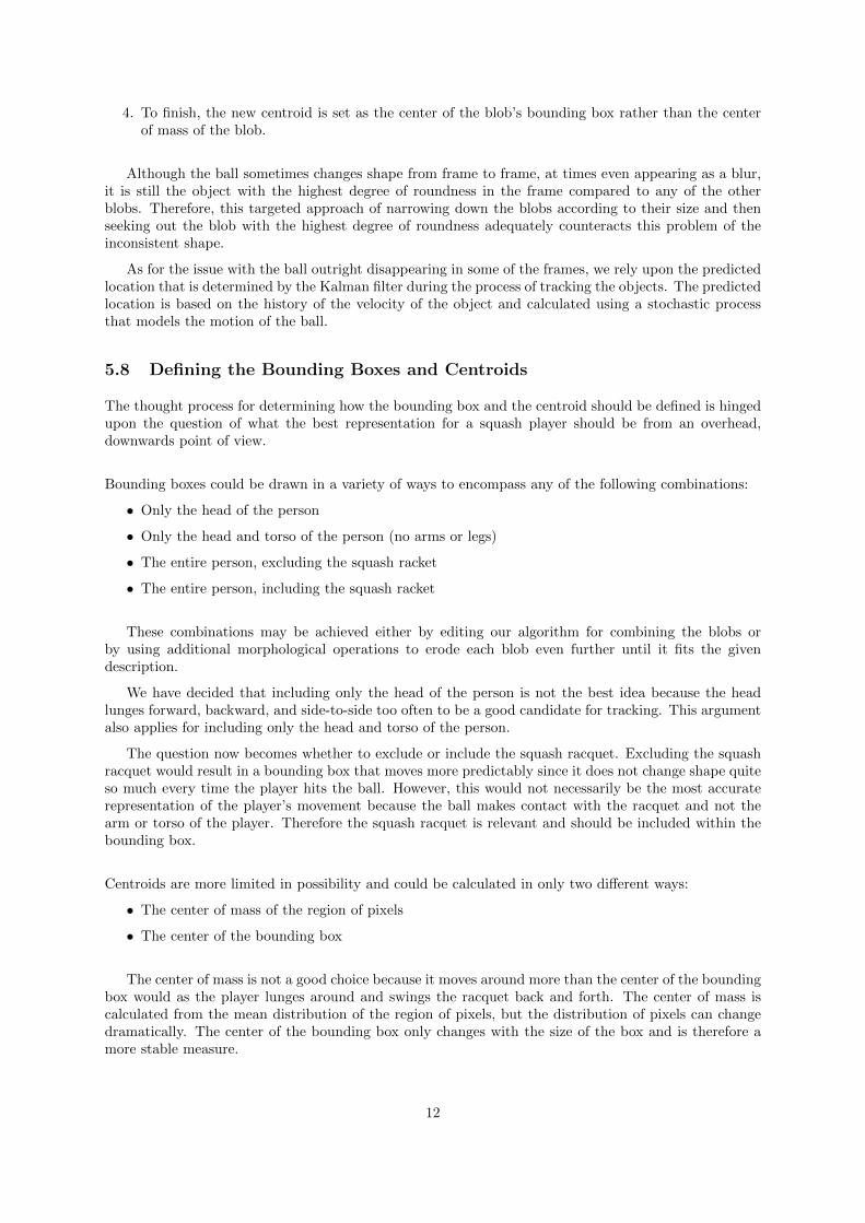
5.8 Defining the Bounding Boxes and Centroids

The thought process for determining how the bounding box and the centroid should be defined is hingedupon the question of what the best representation for a squash player should be from an overhead,downwards point of view.

Bounding boxes could be drawn in a variety of ways to encompass any of the following combinations:

• Only the head of the person

• Only the head and torso of the person (no arms or legs)

• The entire person, excluding the squash racket

• The entire person, including the squash racket

These combinations may be achieved either by editing our algorithm for combining the blobs orby using additional morphological operations to erode each blob even further until it fits the givendescription.

We have decided that including only the head of the person is not the best idea because the headlunges forward, backward, and side-to-side too often to be a good candidate for tracking. This argumentalso applies for including only the head and torso of the person.

The question now becomes whether to exclude or include the squash racquet. Excluding the squashracquet would result in a bounding box that moves more predictably since it does not change shape quiteso much every time the player hits the ball. However, this would not necessarily be the most accuraterepresentation of the player’s movement because the ball makes contact with the racquet and not thearm or torso of the player. Therefore the squash racquet is relevant and should be included within thebounding box.

Centroids are more limited in possibility and could be calculated in only two different ways:

• The center of mass of the region of pixels

• The center of the bounding box

The center of mass is not a good choice because it moves around more than the center of the boundingbox would as the player lunges around and swings the racquet back and forth. The center of mass iscalculated from the mean distribution of the region of pixels, but the distribution of pixels can changedramatically. The center of the bounding box only changes with the size of the box and is therefore amore stable measure.

12

6 TRACKING THE OBJECTS

A “track” is a structure representing a moving object in a video. It contains different fields that are usedto determine the assignment of detections to tracks, the termination of tracks that may no longer exist,and the display of the tracks to the screen. These fields represent the state of a tracked object at a pointin time:

• id: the integer id of the track

• bbox: the bounding box of the track

• kalmanFilter: the object used for motion prediction

• age: # of frames since the track was first detected

• totalV isibleCount: # of total frames in which the track was detected

• consecutiveInvisibleCount: # of consecutive frames where the track was not detected

The tracks are stored in an array, and their fields are continually updated from frame to frame toreflect their new values.

6.1 Track Maintenance

After the objects are detected in each frame of the input video, there are a number of possibilities forhow the array of tracks will be updated. An object detection may be assigned to an existing track,which is then updated to reflect the most recent bounding box, the new predicted motion, and the newframe counts for age and visible count. Otherwise, an object detection may also remain unassigned fromany existing tracks. However, if it has previously been detected before, its associated track will still beupdated to reflect the new frame count for the invisible count since the object has not been assigned forthat frame.

If a track has just been newly created for a new object detection, it will not display the object’sbounding box at first. The bounding box of an object will only be displayed after the object has beentracked for a minimum number of frames, or when the visible count exceeds a certain threshold. Thispreventative measure is to minimize noise from tracks that are created, exist for a brief amount of time,and then quickly deleted afterwards. An example of when this sort of noise might occur is if a trackhas been created but then marked invisible for most of the frames in its lifespan and then consequentlybecomes deleted.

When a track is continually unassigned for multiple frames in a row and the invisible count conse-quently exceeds a certain threshold, the track is then deleted. This is because the object associated withthe deleted track has not been seen for a while and is thus assumed to have left the field of view of thecamera.

6.2 Predicting New Locations of Existing Tracks

Before evaluating the detection objects in the input frame, we use a Kalman filter to predict the nextlocation of each existing track. The Kalman filter calculates the predicted centroid and then shifts theassociated bounding box of the track so that its center is equal to the predicted location. Hence, thesesteps preserve our chosen definition of a centroid since it is still made to be the exact center of thebounding box.

The Kalman filter is an estimator used to calculate the solution to a stochastic process without havingprecise knowledge of the underlying dynamic system.14 It predicts the state of the dynamic system from

14”Estimate System Measurements and States Using Kalman Filter.” MATLAB Documentation Center.http://www.mathworks.com/help/dsp/ref/dsp.kalmanfilter-class.html#bt0lhkw-3

13

a series of incomplete and noisy measurements, such as when the object is not detected or when theobject is confused with another similar moving object. The stochastic process that is implemented isdefined by the following equations:15

xk = Axk−1 + wk−1

zk = Hxk + vk

In these Markov chain equations, it is only necessary to know the immediate prior state of the systemto assess the current state. To define the variables in the first equation, x is the state of the stochasticprocess, k is the kth step of the process, A is the state transition matrix, and w is the process noise.In the second equation, z is the measurement equation that takes measurement xk as an input, H isthe measurement matrix, and v is the measurement noise. The values of matrices A and H are thefollowing:15

A =

∣∣∣∣∣∣∣∣∣∣∣∣

1 0 1 0 0 00 1 0 1 0 00 0 1 0 0 00 0 0 1 0 00 0 0 0 1 00 0 0 0 0 1

∣∣∣∣∣∣∣∣∣∣∣∣H =

∣∣∣∣∣∣∣∣1 0 0 0 0 00 1 0 0 0 00 0 0 0 1 00 0 0 0 0 1

∣∣∣∣∣∣∣∣In our project, the Kalman filter implements a motion model of constant velocity. The alternativeoption available is implementing a motion model of constant acceleration. We have selected the model ofconstant velocity because the overhead point of view means that the only velocity that matters is parallelto the floor in the x-direction, and the only acceleration parallel to the floor would be wind resistance -which is minimal in an enclosed, indoors environment. Constant acceleration would only apply if therewas a behind point of view instead because the acceleration in the y-direction would then be the constantforce of gravity.16

Obviously implementing a motion model of constant velocity is not a perfect representation of themoving objects either, since objects typically do not move with constant velocity.17 We have adjusted forthis imperfect assumption by setting the motion noise parameter, which specifies the amount of alloweddeviation from the ideal motion model. Increasing the motion noise parameter leads the Kalman filterto depend more on incoming measurements rather than its internal state. For our project, we haveconfigured the motion noise to be [100, 25] to rely more heavily on incoming measurements of locationand velocity.

When an object temporarily happens to be missing in a frame, there is no current measurement avail-able for the object so the Kalman filter calculates the predicted centroid based solely on the informationfrom the previous state of the object.

This motion prediction step is important for the next step of assigning detections to tracks, sincethe Kalman filter’s predictions and confidence levels are used to determine the likelihood of each objectdetection being assigned to a track. The confidence levels indicate the confidence of the Kalman predic-tions for the centroids.

15”Predict or Estimate States of Dynamic Systems.” MATLAB Documentation Center.http://www.mathworks.com/help/dsp/ref/kalmanfilter.html

16”Newton’s Law of Universal Gravitation.” The Physics Classroom. http://www.physicsclassroom.com/class/circles/u6l3c.cfm17”Instantaneous Velocity: A Graphical Representation.” Boundless Education. https://www.boundless.com/physics/

kinematics/speed-and-velocity/instananeous-velocity-a-graphical-interpretation

14

6.3 Assigning Detections to Tracks

The way that an object detection is assigned to one of the existing tracks is by calculating the “cost” ofassigning the detection to each existing track and then selecting the track with the minimum cost. Thecost is calculated as a function of:

• The Euclidean distance between the track’s predicted centroid and the detection’s actual centroid

• The confidence of the Kalman prediction - which is outputted by the Kalman filter

Basically, the contributing factors of the cost function show that a detection is more likely to beassigned to a track based on how closely the centroid of the detection matches the Kalman filter’spredicted centroid of a track. The higher the confidence level of the prediction, the greater the likelihoodof assignment.

After the cost of assignment is calculated for each possible pair of (existing track, object detection),the results are stored in a m x n cost matrix, where m is the number of tracks and n is the numberof detections. This cost matrix will be the first input for the function that we use to solve the trackassignment problem, which entails finding the optimal pairings between tracks and detections that willminimize the total cost.

Next, a cost of not assigning any detections to a track is selected. This particular cost of non-assigmentessentially helps to determine whether or not it makes sense to create a new track for a detection thatmay possibly be for a new object, rather than assigning the detection to a corresponding existing trackif it is not a new object. The consequences of assigning an object to the wrong track would be corrupteddata analysis.

The cost of non-assignment measure is set through trial and error. If the cost is set too low, thereis a greater tendency towards creating a new track which may lead to track fragmentation where theremay be multiple tracks that are associated with the same object. On the other hand, if the cost is settoo high then there is a greater tendency towards assigning detections to existing tracks which may leadto the opposite problem where there may be one single track that is associated with multiple movingobjects. This cost of non-assignment will be the second input for the function that we use to solve thetrack assignment problem.

After trying out several values we have chosen a cost of non-assignment of 40. Lower values of thisparameter have resulted in multiple bounding boxes drawn over the same player, whereas higher valueshave resulted in no bounding boxes at all. A cost of non-assignment of 40 results in one bounding boxand one track, per player.

Finally, the “assignDetectionsToTracks” function takes in the two inputs - the cost matrix and thecost of non-assignment - to solve the assignment problem and then returns three outputs that will beused to update the tracks array:

• The assignments of detections to tracks

• The unassigned tracks

• The unassigned detections

6.4 Updating Assigned Tracks

Once an object detection has been assigned to an existing track, the track needs to be updated to reflectthe detection’s current information. First, we correct the track’s location to the object detection’s actuallocation. Next, we store the new bounding box that is based on the object’s actual location. Finally, theframe counts also need to be changed: the total visible count is incremented by 1, the age of the trackis incremented by 1, and the consecutive invisible count is reset to 0.

15

6.5 Updating Unassigned Tracks

If an existing track has not been assigned a detection for a certain frame, the frame counts for that trackwill still be changed so that the age of the track is incremented by 1 and the consecutive invisible countis incremented by 1.

6.6 Deleting Lost Tracks

Tracks will be deleted if they have too a consecutive invisible count that is too high exceeds a certainthreshold. Even if the consecutive invisible count is 0, a track could still be deleted if the difference(age - total visible count) also exceeds the threshold since this means that the track has been countedas invisible numerous times.

6.7 Creating New Tracks

New tracks are created when there is an object detection that is not assigned to any existing track. Weassume that these detections are new moving objects that have not been seen before. Our algorithm tocombine blobs greatly reduces the likelihood of unnecessarily creating new tracks because it minimizesthe amount of noise in the frame and ensures that there is only one blob and one track created for eachsquash player.

6.8 Displaying Tracking Results

After track maintenance is completed, the tracks are displayed to the screen. The bounding boxes fromeach track are drawn in both video players - one that displays the original video input and one thatdisplays the binary mask.

7 SPORTS ANALYTICS

Now that the video footage has been processed and the objects have been detected and tracked, theoutput .csv file of the (x, y) coordinates of the squash players will be evaluated by another program thatwill create another output analytics file.

7.1 Industry Overview

As previously mentioned in the introduction, sports analytics is already established in some sports suchas basketball and baseball. The statistics provided by these analytics are used by coaches to informplayers how to improve their game. The statistics are also available to the mass public, who even createformulas that weight certain statistical metrics that are deemed most important.

The National Basketball Association uses statistics such as effective field goal percentage (shootingpercentage), turnovers per possession, offensive rebounding percentage, and number of times gettingto the foul line.18 Some innovators are attempting similar precision technique analysis tools such as94Fifty’s ”smart basketball” that uses a bluetooth enabled accelerometer and gyroscope system to reportacceleration, impulse, spin, and more. The software then computes technical attributes such as ballhandling ability, shot arc, shot speed, shot backspin, etc.19

18Meehan, Jeff. ”Back to the Basics: Four Factors in Basketball.” Sports Analytics Blog. http://sportsanalyticsblog.com/articles/back-to-the-basics-four-factors-in-basketball

19”Learn More: 94Fifty Smart Sensor Basketball.” 94Fifty. http://shop.94fifty.com/pages/learn-more

16

The Major League of Baseball uses statistics such as batting average, number of home runs, numberof strikes, plate appearances, and contact rate.20 Innovative software is also being developed in this spaceto use broadcast provided footage in order to track motions of the baseball and players and determinestatistics regarding individual plays.21

7.2 Squash Overview

Squash game strategy is highly dependent on court positioning, player speed, and the player’s ability tomake and retrieve shots.

Court positioning is important because an ideal positioning on the court can greatly reduce theamount of distance that players need to travel and therefore ensures that they tire less quickly. A keystrategy called ”dominating the T” gives a squash player quick access to any part of the court in orderto retrieve the opponent’s shot. This strategy involves moving towards the intersecting red lines inthe center of the court after returning a shot and taking control over this ideal location to be betterpositioned to retrieve subsequent shots.

Player speed is essential for covering a greater court area and also for recovering quickly after makinga shot. A player that has good agility would be able to return a well-placed shot and then quickly reversedirections for the next one. The opponent’s goal is to place the ball in a region that is far in distancefrom the player as well as in an area that is in the opposite direction of the player’s momentum, so beingquick on their feet is important for players to execute a good play or risk losing the point. Anotherpossible consequence of not moving quickly enough is accidentally causing an interference violation andpotentially losing the point.

The ability to make and retrieve shots is crucial for winning points from both offensive and defensiveperspectives. Shot placement on the front wall is directly associated with scoring. If the opponent failsto return a shot, the player who delivered the final shot wins the point. A player that is highly skilledat making powerful shots and also adept at receiving them maximizes the likelihood of winning pointsand winning the overall squash match.

7.3 Squash Analytics

In light of the fact that a Google search for ”squash analytics” yields no relevant results, it is clear thatthere is much room for development in terms of advancing sports analytics for squash. Based on theabove overview for squash, the sport’s game strategy can be quantified on a similar level to any othersport with established sports analytical systems.

After consulting with Jack Wyant, the head coach of the Penn Varsity Squash team, we have a goodsense for which statistics would be the most beneficial for analyzing squash performance. Some of thedesired analytics include:

• average location on the squash court

• average distance traveled

• average speed of the player

• hit rate (percentage of shots retrieved)

• scoring ability (percentage of winning shots)

• total number of shots made

20Rosen, Jacob. ”Roundup: Baseball stats and salaries, basketball, and more.” Sports Analytics Blog. http://sportsanalyticsblog.com/articles/roundup-baseball-stats-and-salaries-basketball-and-more

21Perry, Dayn. ”Innovative ’player tracking’ has arrived, and it is beautiful.” CBS Sports. http://www.cbssports.com/mlb/eye-on-baseball/24462312/video-innovative-player-tracking-has-arrived-and-it-is-beautiful

17

7.4 Project Scope

We have defined the scope for our data analysis to focus on the first three metrics in the above listof analytical metrics: average location, average distance traveled, and average speed. These analyticalmetrics are focused on the movements of the players rather than the ball. Our coordinates data is goodfor this form of analysis since our program’s mechanism for detecting and tracking each squash player isfairly consistent.

We have also included a calculation for the direction of movement to provide analytics on whichdirection a player is traveling at every point in time, measured in degrees relative to the court lines. Thisadditional calculation would be simple to perform since the required data is the same as for calculatingthe first three metrics. Information about movement direction may be useful for determining playeragility.

We will leave the remaining analytical metrics for future work since they are focused on the movementsof the ball and require accurate location information about the ball. However, our mechanism fordetecting and tracking the ball is not yet on the level of consistency necessary to perform reliableanalysis.

8 CODE OVERVIEW - PART 2

In the program written for coordinate-based data analysis, the main method first opens the .csv filecontaining the (x, y) coordinates data created by the first program. Then it creates four n x 2 matricesto store the location data and the calculated metrics, which will be referenced later on at the end of theprogram when creating the output .csv file.

The program begins parsing through the file of coordinates. It maintains a variable ”prevCoordinate”to store the previous location coordinate for the purposes of calculating the analytical metrics. In eachiteration, the program inputs the current pair of coordinates along with the previous pair of coordinatesinto one method to perform the movement analysis and a second method to create and build the heatmap.

The method for movement analysis uses the two coordinate inputs to calculate the three desiredmetrics: distance traveled, the speed of the player, and the direction of the player’s movement. Themethod then returns these analytics data points to be saved in their respective n x 2 matrices as well asto be recorded in the output file.

The method for building a heat map uses the coordinate input for the current state to draw a pointrepresenting the current location of the player onto an image representation of a squash court that hasbeen drawn by the program. One point will be drawn onto the same image in each iteration so thattogether the drawn points will give a visual of each player’s path over time. The image is continuallyupdated until the file reader terminates.

After the program finishes evaluating each coordinate in the input file, it uses the data stored in thematrices to calculate the average location, the average distance traveled, and the average speed of theplayer. The final output .csv file will contain all of the data in the matrices from the entire duration ofthe video footage, as well as the average statistics calculated at the end.

9 MOVEMENT ANALYSIS

Given the two input coordinates, in terms of feet, we now have the object’s current location as well asits past location from the immediate prior state. The calculation of the analytical metrics is a relativelystraightforward process. As mentioned previously in Section 2.2, the formulas used in the calculationsare the following:

18

• Distance traveled: D =√

(x2 − x1)2 + (y2 − y1)2

• Speed of player: s = D/t, t ≈ 0.0083 seconds

• Direction of movement: θ = tan−1( y2−y1

x2−x1)

However, the main challenge we have faced is a result of some inconsistencies that only occur infre-quently in the mechanism for detecting and tracking the player. For a few brief stints in the video, thebounding box temporarily shifts from encompassing the entire body of the player to encompassing onlythe head.

The implications of this tracking error is that the centroid of the associated track shifts dramaticallyfrom the center of the body to the center of the head. Consequently, in the span of less than a second(≈ 0.0083 seconds), the movement analysis errantly determines that the player has traveled much furtherthan it has actually moved in reality. So even though this tracking error may occur only a few times,the data analysis becomes corrupted.

To counter this problem, we have decided to reduce the noise by lowering the frequency of the inputand only measuring the locations of the players every couple of frames. In addition to this strategy, wehave also set a maximum distance threshold so that the program does not consider distance values thatfurther exceed this threshold and are likely erroneous.

10 CREATION OF HEAT MAP

To create the heat map, the first step is to construct a new background image of the squash courtsince the video frame does not reflect the real proportions or orientation of an actual real-world court.The u x v dimension of the video frame is 1280 x 720 pixels with the court turned sideways, in thecounterclockwise direction. So the court is 1280 pixels in horizontal length and 720 pixels in verticalwidth.

To create the background image of the squash court, we create a new blank image and draw a newsquash court that maintains the same length to width ratio as well as the same vertical orientation asan actual court. The true x x y proportion of the court is 32 x 21 feet, or 32 feet in vertical length and21 feet in horizontal width.

To find the correct pixel dimensions for the new image that we aim to create, we consider the factthat the computer frame has a maximum vertical range of v =720 pixels and thus set a relation thatfinds the corresponding horizontal width, u, in pixels in the same proportion as an actual court:

720

u=

32

21

The new horizontal width, u, turns out to be approximately 473 pixels.

Since the origin in the video frame is in the top left-hand corner of the image and the origin for theactual court is at the intersecting court lines, the real-world coordinates can be converted back into pixelvalues (u, v) using the following relations:

u = 10.5 +473

21x

v = 18− 720

32y

The ratios473

21and

720

32are used to adjust for the difference in scale.

19

With these pixel values, we plot one red circle and one blue circle onto the new image to representeach player’s location. Originally a white canvas, the replicated image of the squash court is eventuallypopulated with additional circle points after processing each frame of the input video.

It is important to note that we have made a key assumption that it is safe to assume that the centerof each bounding box is accurate enough to represent each player’s location for that particular frame.This is certainly an approximation, albeit one that we believe is accurate enough given the limitationsof the technology.

11 FUTURE WORK

Our project has tackled a significant issue head-on by addressing the need for quantitative data analysisfor the sport of squash. It is hard to reconcile the fact that squash coaches still rely on the same methodsof instruction that they have depended on for the past decade, even while other sports are advancingforwards in terms of analytics innovation.

Jack Wyant is wholeheartedly involved in the squash program at Penn and has lamented that he canmerely ”throw his hands in the air” when coaching without the use of analytics, and he wishes he couldhave hard statistics to show to the team.

Going forward, there is significant work that can be further done for this product to be fully adoptedand supported by U.S. Squash, as they indicated they would:

1. First of all, our algorithms must be able to handle clothing of all colors. Currently, it is difficultfor the code to detect players if they are wearing a white shirt. This is because during backgroundsubtraction, we are subtracting one white pixel from another which results in a value of 0. Thereforethe shirt will incorrectly be categorized as the background and will therefore not be displayed aspart of the squash player in the binary mask.

2. The ball tracking capabilities need to be improved. What is so challenging is that the ball is notvisible for much of the time, even after applying separate morphological operations specificallyoriented towards detecting the ball. Future experiments should utilize a high speed camera thatis specifically designed for capturing fast-moving objects and thus has the capacity to acquire thecorrect input.

3. There is more analysis that can be done from successful ball tracking. It would then not only bepossible to determine analytical metrics such as the hit rate and scoring ability of a player, butalso to figure out the type of shot that the player has hit. With that information we could thendetermine a player’s shot quality.

For example, if we determine that a player hit a straight drive, then we know where exactly itshould land on the court to be a ”good shot.” Hence, we could quantify the quality of a shot thata player has hit and use this measure to keep track of quality improvements. This kind of analysiswould be immensely useful for any squash player.

4. An even more difficult challenge is automatically determining when a point has ended and whena point has started. Currently, we have recorded a large quantity of video such that each videoonly contains footage for one individual point. Ideally, a program should be able to take one longvideo of an entire squash game and automatically determine when a point has started and whenthe point has ended.

5. Finally, a more refined system for data input and output would be necessary to package theproduct for end-consumers. What we have produced already has impactful analysis. However, tocommercialize it, it will need a functional user interface. For this future product, we envision forrecorded video to be automatically integrated and then with the resulting analysis emailed to theuser when the computation has finished.

20

12 APPENDIX

Figure 1: The ”ginput” function prompts the user to input 6 coordinates → 4 to designate the courtboundaries, 1 to designate the court center, and 1 to designate the upper right-hand corner of the court.

Figure 2: Our blob analysis algorithm draws a single bounding box around each squash player, whileignoring the unrelated objects around the court.

21

Figure 3: The background subtraction creates a binary mask of the original frame, which is used todetect the players. Note that the ball is not visible in this mask because the mask has been createdspecifically to find the players, not the ball, using the morphological operations ”imopen”, ”imclose”,and ”imfill”.

Figure 4: From this heat map, here is some example analysis: you can see that Player 2 (marked by bluecircles) is clearly standing too far back in the court after receiving the serve. Ideally, Player 2 should bestanding at the ”T”, the place where the two red lines connect, so that there is less distance to travelwhen retrieving the next shot. Any coach would be able to look at this imagery and offer players theadvice that they must stand at least a few feet further up on the squash court. This advice alone couldsignificantly reduce how tired players feel during a match, thus improving their performance significantly.

22