Embed Size (px)
Citation preview
SQL Server In-Memory OLTP Internals Overview for CTP2
SQL Server Technical Article
Writer: Kalen Delaney
Technical Reviewers: Kevin Liu, Sunil Agarwal, Jos de Bruijn, Kevin Farlee, Mike Zwilling,
Craig Freedman, Mike Weiner, Cristian Diaconu, Pooja Harjani, Paul Larson, David Schwartz
Published: October 2013
Applies to: SQL Server 2014 CTP2
Summary: In-Memory OLTP (project “Hekaton”) is a new database engine component, fully integrated into
SQL Server. It is optimized for OLTP workloads accessing memory resident data. In-Memory
OLTP allows OLTP workloads to achieve significant improvements in performance, and
reduction in processing time. Tables can be declared as ‘memory optimized’ to enable In-
Memory OLTP’s capabilities. Memory-optimized tables are fully transactional and can be
accessed using Transact-SQL. Transact-SQL stored procedures can be compiled to machine
code for further performance improvements on memory-optimized tables. The engine is
designed for high concurrency and blocking is minimal.

2
Copyright
This document is provided “as-is”. Information and views expressed in this document, including URL and
other Internet Web site references, may change without notice. You bear the risk of using it.
This document does not provide you with any legal rights to any intellectual property in any Microsoft
product. You may copy and use this document for your internal, reference purposes.
© 2013 Microsoft. All rights reserved.

3
Contents Introduction .................................................................................................................................................. 5
Design Considerations and Purpose ............................................................................................................. 5
Terminology .................................................................................................................................................. 6
Overview of Functionality ............................................................................................................................. 6
What’s Special About In-Memory OLTP? ...................................................................................................... 6
Memory-optimized tables ........................................................................................................................ 7
Indexes on memory-optimized tables ...................................................................................................... 8
Concurrency improvements ..................................................................................................................... 8
Natively Compiled Stored Procedures ...................................................................................................... 8
Is In-Memory OLTP just an improved DBCC PINTABLE? ........................................................................... 8
Offerings from competitors ...................................................................................................................... 9
Using In-Memory OLTP ............................................................................................................................... 10
Creating Databases ................................................................................................................................. 10
Creating Tables........................................................................................................................................ 11
Row and Index Storage ............................................................................................................................... 12
Rows ........................................................................................................................................................ 13
Row header ......................................................................................................................................... 13
Payload area ........................................................................................................................................ 14
Indexes On Memory-Optimized Tables .................................................................................................. 14
Hash Indexes ....................................................................................................................................... 15
Range Indexes ..................................................................................................................................... 17
Data Operations ...................................................................................................................................... 21
Isolation Levels Allowed with Memory-Optimized Tables .................................................................. 22
Deleting ............................................................................................................................................... 23
Updating and Inserting ....................................................................................................................... 23
Reading ............................................................................................................................................... 24
Validation ............................................................................................................................................ 25
T-SQL Support ..................................................................................................................................... 26
Garbage Collection of Rows in Memory ............................................................................................. 27
Transaction Isolation and Concurrency Management ................................................................................ 28
Checkpoint and Recovery ........................................................................................................................... 30
Transaction Logging ................................................................................................................................ 31
Checkpoint .............................................................................................................................................. 34

4
Checkpoint Files .................................................................................................................................. 35
The Checkpoint Process ...................................................................................................................... 35
Merging Checkpoint Files ........................................................................................................................ 35
Automatic Merge ................................................................................................................................ 36
Manual Merge sys.sp_xtp_merge_checkpoint_files .......................................................................... 36
Garbage Collection of Checkpoint Files .............................................................................................. 37
Recovery.................................................................................................................................................. 38
Native Compilation of Tables and Stored Procedures ................................................................................ 39
What is native compilation? ................................................................................................................... 39
Maintenance of DLLs............................................................................................................................... 39
Native compilation of tables ................................................................................................................... 40
Native compilation of stored procedures ............................................................................................... 40
Compilation and Query Processing ..................................................................................................... 41
SQL Server Feature Support ........................................................................................................................ 42
Manageability Experience ....................................................................................................................... 42
Metadata ..................................................................................................................................................... 43
Catalog Views .......................................................................................................................................... 43
Dynamic Management Objects ............................................................................................................... 43
XEvents .................................................................................................................................................... 44
Performance Counters ............................................................................................................................ 44
Memory Usage Report ............................................................................................................................ 44
Memory Requirements ........................................................................................................................... 45
Managing Memory with the Resource Governor ............................................................................... 46
Using AMR ................................................................................................................................................... 47
Summary ..................................................................................................................................................... 48
For more information: ................................................................................................................................ 48

5
Introduction SQL Server was originally designed at a time when it could be assumed that main memory was very
expensive, so data needed to reside on disk except when it was actually needed for processing. This
assumption is no longer valid as memory prices have dropped enormously over the last 30 years. At the
same time, multi-core servers have become affordable, so that today one can buy a server with 32 cores
and 1TB of memory for under $50K. Since many, if not most, of the OLTP databases in production can fit
entirely in 1TB, we need to re-evaluate the benefit of storing data on disk and incurring the I/O expense
when the data needs to be read into memory to be processed. In addition, OLTP databases also incur
expenses when this data is updated and needs to be written back out to disk. Memory-optimized tables
are stored completely differently than disk-based tables and these new data structures allow the data to
be accessed and processed much more efficiently.
Because of this trend to much more available memory and many more cores, the SQL Server team at
Microsoft began building a database engine optimized for large main memories and many-core CPUs.
This paper gives a technical overview of this new database engine feature: In-Memory OLTP.
For more information about In-Memory OLTP, see In-Memory OLTP (In-Memory Optimization).
Design Considerations and Purpose The move to produce a true main-memory database has been driven by three basic needs: 1) fitting
most or all of data required by a workload into main-memory, 2) lower latency time for data operations,
and 3) specialized database engines that target specific types of workloads need to be tuned just for
those workloads. Moore’s law has impacted the cost of memory allowing for main memories to be large
enough to satisfy (1) and to partially satisfy (2). (Larger memories reduce latency for reads, but don’t
affect the latency required for writes to disk needed by traditional database systems). Other features of
In-Memory OLTP allow for greatly improved latency for data modification operations. The need for
specialized database engines is driven by the recognition that systems designed for a particular class of
workload can frequently out-perform more general purpose systems by a factor of 10 or more. Most
specialized systems, including those for CEP (complex event processing), DW/BI and OLTP, optimize data
structures and algorithms by focusing on in-memory structures.
Microsoft’s reason for creating In-Memory OLTP comes mainly from this fact that main memory sizes
are growing at a rapid rate and becoming less expensive. In addition, because of the near universality of
64 bit architectures and multicore processors, it is not unreasonable to think that most, if not all, OLTP
databases or the entire performance sensitive working dataset could reside entirely in memory. Many of
the largest financial, online retail and airline reservation systems fall between 500GB to 5TB with
working sets that are significantly smaller. As of 2012, even a two socket server could hold 2TB of DRAM
using 32GB DIMMS (such as IBM x3680 X5). Looking further ahead, it’s entirely possible that in a few
years you’ll be able to build distributed DRAM based systems with capacities of 1-10 Petabytes at a cost
less than $5/GB. It is also only a question of time before non-volatile RAM becomes viable.
If most or all of an application’s data is able to be entirely memory resident, the costing rules that the
SQL Server optimizer has used since the very first version become almost completely obsolete, because
the rules assume all pages accessed can potentially require a physical read from disk. If there is no
reading from disk required, the optimizer can use a different costing algorithm. In addition, if there is no

6
wait time required for disk reads, other wait statistics, such as waiting for locks to be released, waiting
for latches to be available, or waiting for log writes to complete, can become disproportionately large.
In-Memory OLTP addresses all these issues. In-Memory OLTP removes the issues of waiting for locks to
be released, using a new type of multi-version optimistic concurrency control. It reduces the delays of
waiting for log writes by generating far less log data and needing fewer log writes.
Terminology SQL Server 2014’s In-Memory OLTP feature refers to a suite of technologies for working with memory-
optimized tables. The alternative to memory-optimized tables will be referred to as disk-based tables,
which SQL Server has always provided. Terms to be used include:
Memory-optimized tables refer to tables using the new data structures added as part of In-
Memory OLTP, and will be described in detail in this paper.
Disk-based tables refer to the alternative to memory-optimized tables, and use the data
structures that SQL Server has always used, with pages of 8K that need to be read from and
written to disk as a unit.
Natively compiled stored procedures refer to an object type supported by In-Memory OLTP that
is compiled to machine code and has the potential to increase performance even further than
just using memory-optimized tables. The alternative is interpreted Transact-SQL stored
procedures, which is what SQL Server has always used. Natively compiled stored procedures can
only reference memory-optimized tables.
Cross-container transactions refer to transactions that reference both memory-optimized tables
and disk-based tables.
Interop refers to interpreted Transact-SQL that references memory-optimized tables
Overview of Functionality During most of your data processing operations with In-Memory OLTP, you may be unaware that you
are working with memory-optimized tables rather than disk-based tables. However, SQL Server is
working with your data very differently if it is stored in memory-optimized tables. In this section, we’ll
look at an overview of how In-Memory OLTP operations and data are handled differently than disk-
based operations and data in SQL Server. We’ll also briefly mention some of the memory optimized
database solutions from competitors and point out how SQL Server In-Memory OLTP is different from
them.
What’s Special About In-Memory OLTP? Although In-Memory OLTP is integrated with the SQL Server relational engine, and can be accessed
using the same interfaces transparently, its internal behavior and capabilities are very different. Figure
1 gives an overview of the SQL Server engine with the In-Memory OLTP components.

7
Figure 1The SQL Server engine including the In-Memory OLTP component
Notice that the client application connects to the TDS Handler the same way for memory-optimized
tables or disk-based tables, whether it will be calling natively compiled stored procedures or interpreted
Transact-SQL. You can see that interpreted Transact-SQL can access memory-optimized tables using
the interop capabilities, but that natively compiled stored procedures can only access memory-
optimized tables.
Memory-optimized tables The most important difference between memory-optimized tables and disk-based tables is that pages
do not need to be read into cache from disk when the memory-optimized tables are accessed. All the
data is stored in memory, all the time. A set of checkpoint files (data and delta file pairs), which are only
used for recovery purposes, is created on files residing in memory-optimized filegroups that keep track
of the changes to the data, and the checkpoint files are append-only.
Operations on memory-optimized tables use the same transaction log that is used for operations on
disk-based tables, and as always, the transaction log is stored on disk. In case of a system crash or server
shutdown, the rows of data in the memory-optimized tables can be recreated from the checkpoint files
and the transaction log.
In-Memory OLTP does provide the option to create a table that is non-durable and not logged using an
option called SCHEMA_ONLY. As the option indicates, the table schema will be durable, even though the
data is not. These tables do not require any IO operations during transaction processing, but the data is
only available in memory while SQL Server is running. In the event of a SQL Server shutdown or an

8
AlwaysOn Availabilty Group failover, the data in these tables is lost. The tables will be recreated when
the database they belong to is recovered, but there will be no data in the tables. These tables could be
useful, for example, as staging tables in ETL scenarios or for storing Web server session state. Although
the data is not durable, operations on these tables meet all the other transactional requirements; they
are atomic, isolated, and consistent. We’ll see the syntax for creating a non-durable table in the section
on Creating Tables.
Indexes on memory-optimized tables Indexes on memory-optimized tables are not stored as traditional B-trees. Memory-optimized tables
support hash indexes, stored as hash tables with linked lists connecting all the rows that hash to the
same value and range indexes, which for memory-optimized tables are stored using special Bw-trees.
Nonclustered indexes on memory-optimized tables were not available prior to CTP2. ,
Every memory-optimized table must have at least one index, because it is the indexes that combine all
the rows into a single table. Memory-optimized tables are never stored as unorganized sets of rows, like
a disk-based table heap is stored.
Indexes are never stored on disk, and are not reflected in the on-disk checkpoint files and operations on
indexes are never logged. The indexes are maintained automatically during all modification operations
on memory-optimized tables, just like b-tree indexes on disk-based tables, but in case of a SQL Server
restart, the indexes on the memory-optimized tables are rebuilt as the data is streamed into memory.
Concurrency improvements When accessing memory-optimized tables, SQL Server implements an optimistic multi-version
concurrency control. Although SQL Server has previously been described as supporting optimistic
concurrency control with the snapshot-based isolation levels introduced in SQL Server 2005, these so-
called optimistic methods do acquire locks during data modification operations. For memory-optimized
tables, there are no locks acquired, and thus no waiting because of blocking.
Note that this does not mean that there is no possibility of waiting when using memory-optimized
tables. There are other wait types, such as waiting for a log write to complete at the end of a
transaction. However, logging when making changes to memory-optimized tables is much more efficient
than logging for disk-based tables, so the wait times will be much shorter. And there never will be any
waits for reading data from disk, and no waits for locks on data rows.
Natively Compiled Stored Procedures The best execution performance is obtained when using natively compiled stored procedures with
memory-optimized tables. However, there are limitations on the Transact-SQL language constructs that
are allowed inside a natively compiled stored procedure, compared to the rich feature set available with
interpreted code. In addition, natively compiled stored procedures can only access memory-optimized
tables and cannot reference disk-based tables.
Is In-Memory OLTP just an improved DBCC PINTABLE? DBCC PINTABLE was a feature available in older versions of SQL Server that would not remove any data
pages from a “pinned” table from memory, once those pages were read from disk. The pages did need

9
to be read in initially, so there was always a cost for page reads the first time such a table was accessed.
These pinned tables were no different than any other disk-based tables. They required the same amount
of locking, latching and logging and they used the same index structures, which also required locking
and logging. In-Memory OLTP memory-optimized tables are completely different than SQL Server disk-
based tables, they use different data and index structures, no locking is used and logging changes to
these memory-optimized tables is much more efficient that logging changes to disk-based tables.
Offerings from competitors For processing OLTP data, there are two types of specialized engines. The first are main-memory
databases. Oracle has TimesTen, IBM has SolidDB and there are many others that primarily target the
embedded DB space. The second are applications caches or key-value stores (for example, Velocity –
App Fabric Cache and Gigaspaces) that leverage app and middle-tier memory to offload work from the
database system. These caches continue to get more sophisticated and acquire database
capabilities,such as transactions, range indexing, and query capabilities (Gigaspaces already has these
for example). At the same time, database systems are acquiring cache capabilities like high-
performance hash indexes and scale across a cluster of machines (VoltDB is an example). The In-
Memory OLTP engine is meant to offer the best of both of these types of engines. One way to think of
In-Memory OLTP is that it has the performance of a cache and the capability of a database. It supports
storing your tables and indexes in memory, so you can create an entire database to be a complete in-
memory system. It also offers high performance indexes and logging as well as other features to
significantly improve query execution performance.
SQL Server In-Memory OLTP offers the following features that few (or any) of the competitions’
products provide:
Integration between memory-optimized tables and disk-based tables so that the transition to a
memory resident database can be made gradually, creating only your most critical tables and
stored procedure as memory-optimized objects.
Natively compiled stored procedures to improve execution time for basic data manipulation
operations by orders of magnitude
Hash and BW-Tree indexes specifically optimized for main memory access
No storage of data on pages, removing the need for page latches.
True multi-version optimistic concurrency control with no locking or latching for any operations
The most notable difference in design of SQL Server In-Memory OLTP from competitors’ products is the
“interop” integration. In a typical high end OLTP workload, the performance bottle necks are
concentrated in specific areas, such as a small set of tables and stored procedures. It would be costly
and inefficient to force the whole database to be resident in memory. But to date, the other main
competitive products require such an approach. In SQL Server’s case, the high performance and high
contention area can be migrated to In-Memory OLTP, then the operations (stored procedures) on those
memory-optimized tables can be natively compiled to achieve maximum business processing
performance.
One other key In-memory OLTP improvement is to remove the page construct for memory optimized
tables. This fundamentally changes the data operation algorithm from being disk optimized to being

10
memory and cache optimized. As mentioned earlier, one of the confusions about In-Memory OLTP is
that it’s simply “DBCC PINTABLE” as the tables are locked in the bufferpool. However, a lot of the
competitors do still have the page constructs even while the pages are forced to stay in memory. For
example SAP HANA still uses 16KB pages for its in-memory row-store, which would inherently suffer
from page latch contention in a high performance environment.
Using In-Memory OLTP The In-Memory OLTP engine has been available as part of SQL Server 2014 since the June 2013 CTPs.
Installation of In-Memory OLTP is part of the SQL Server setup application. The In-Memory OLTP
components can only be installed with a 64-bit edition of SQL Server 2014, and not available at all with a
32-bit edition.
Creating Databases Any database that will contain memory-optimized tables needs to have at least one
MEMORY_OPTIMIZED_DATA filegroup. These filegroups are used for storing the data and delta file pairs
needed by SQL Server to recover the memory-optimized tables, and although the syntax for creating
them is almost the same as for creating a regular filestream filegroup, it must also specify the option
CONTAINS MEMORY_OPTIMIZED_DATA. Here is an example of a CREATE DATABASE statement for a
database that can support memory-optimized tables:
CREATE DATABASE HKDB ON PRIMARY(NAME = [HKDB_data], FILENAME = 'Q:\data\HKDB_data.mdf', size=500MB), FILEGROUP [SampleDB_mod_fg] CONTAINS MEMORY_OPTIMIZED_DATA (NAME = [HKDB_mod_dir], FILENAME = 'R:\data\HKDB_mod_dir'), (NAME = [HKDB_mod_dir], FILENAME = 'S:\data\HKDB_mod_dir') LOG ON (name = [SampleDB_log], Filename='L:\log\HKDB_log.ldf', size=500MB) COLLATE Latin1_General_100_BIN2;
Note that the above code example creates files on three different drives (Q:, R: and S:) so if you would
like to run this code, you might need to edit the path names to match your system. The names of the
files on R: and S: are identical, so if you create all these files on the same drive you’ll need to
differentiate the two file names.
Also notice a binary collation was specified. At this time, any indexes on memory-optimized tables can
only be on columns using a Windows (non-SQL) BIN2 collation and natively compiled procedures only
support comparisons, sorting, and grouping on those same collations. It can be specified (as done in the
CREATE DATABASE statement above) with a default binary collation for the entire database, or you can
specify the collation for any character data in the CREATE TABLE statement. (You can also specify
collation in a query, for any comparison, sorting or grouping operation.)
It is also possible to add a MEMORY_OPTIMIZED_DATA filegroup to an existing database, and then files
can be added to that filegroup. For example:
11
ALTER DATABASE AdventureWorks2012
ADD FILEGROUP hk_mod CONTAINS MEMORY_OPTIMIZED_DATA;
GO
ALTER DATABASE AdventureWorks2012
ADD FILE (NAME='hk_mod', FILENAME='c:\data\hk_mod')
TO FILEGROUP hk_mod;
GO
Creating Tables The syntax for creating memory-optimized tables is almost identical to the syntax for creating disk-based
tables, with a few restrictions, as well as a few required extensions. Specifying that the table is a
memory-optimized table is done using the MEMORY_OPTIMIZED = ON clause. A memory-optimized
table can only have columns of these supported datatypes:
bit
All integer types: tinyint, smallint, int, bigint
All money types: money, smallmoney
All floating types: float, real
date/time types: datetime, smalldatetime, datetime2, date, time
numeric and decimal types
All non-LOB string types: char(n), varchar(n), nchar(n), nvarchar(n), sysname
Non-LOB binary types: binary(n), varbinary(n) Uniqueidentifier
Note that none of the LOB data types are allowed; there can be no columns of type XML, CLR or the max data types, and all row lengths are limited to 8060 bytes with no off-row data. In fact, the 8060 byte limit is enforced at table-creation time, so unlike a disk-based table, a memory-optimized tables with two varchar(5000) columns could not be created.
A memory-optimized table can be defined with one of two DURABILITY values: SCHEMA_AND_DATA or
SCHEMA_ONLY with the former being the default. A memory-optimized table defined with
DURABILITY=SCHEMA_ONLY, which means that changes to the table’s data are not logged and the data
in the table is not persisted on disk. However, the schema is persisted as part of the database metadata,
so the empty table will be available after the database is recovered during a SQL Server restart.
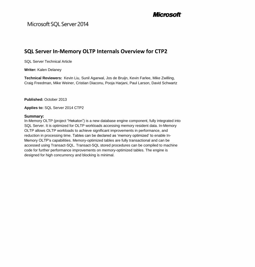
As mentioned earlier, a memory-optimized table must always have at least one index but this
requirement could be satisfied with the index created automatically to support a primary key constraint.
All tables except for those created with the SCHEMA_ONLY option must have a declared primary key. At
least one index must be declared to support a PRIMARY KEY constraint. The following example shows a
PRIMARY KEY index created as a HASH index, for which a bucket count must also be specified. A few
guidelines for choosing a value for the bucket count will be mentioned when discussing details of hash
index storage.
Single-column indexes may be created in line with the column definition in the CREATE TABLE
statement, as shown below. ). The BUCKET_COUNT attribute will be discussed in the section on Hash
Indexes.
12
CREATE TABLE T1 ( [Name] varchar(32) not null PRIMARY KEY NONCLUSTERED HASH WITH (BUCKET_COUNT = 100000), [City] varchar(32) null, [State_Province] varchar(32) null, [LastModified] datetime not null, ) WITH (MEMORY_OPTIMIZED = ON, DURABILITY = SCHEMA_AND_DATA);
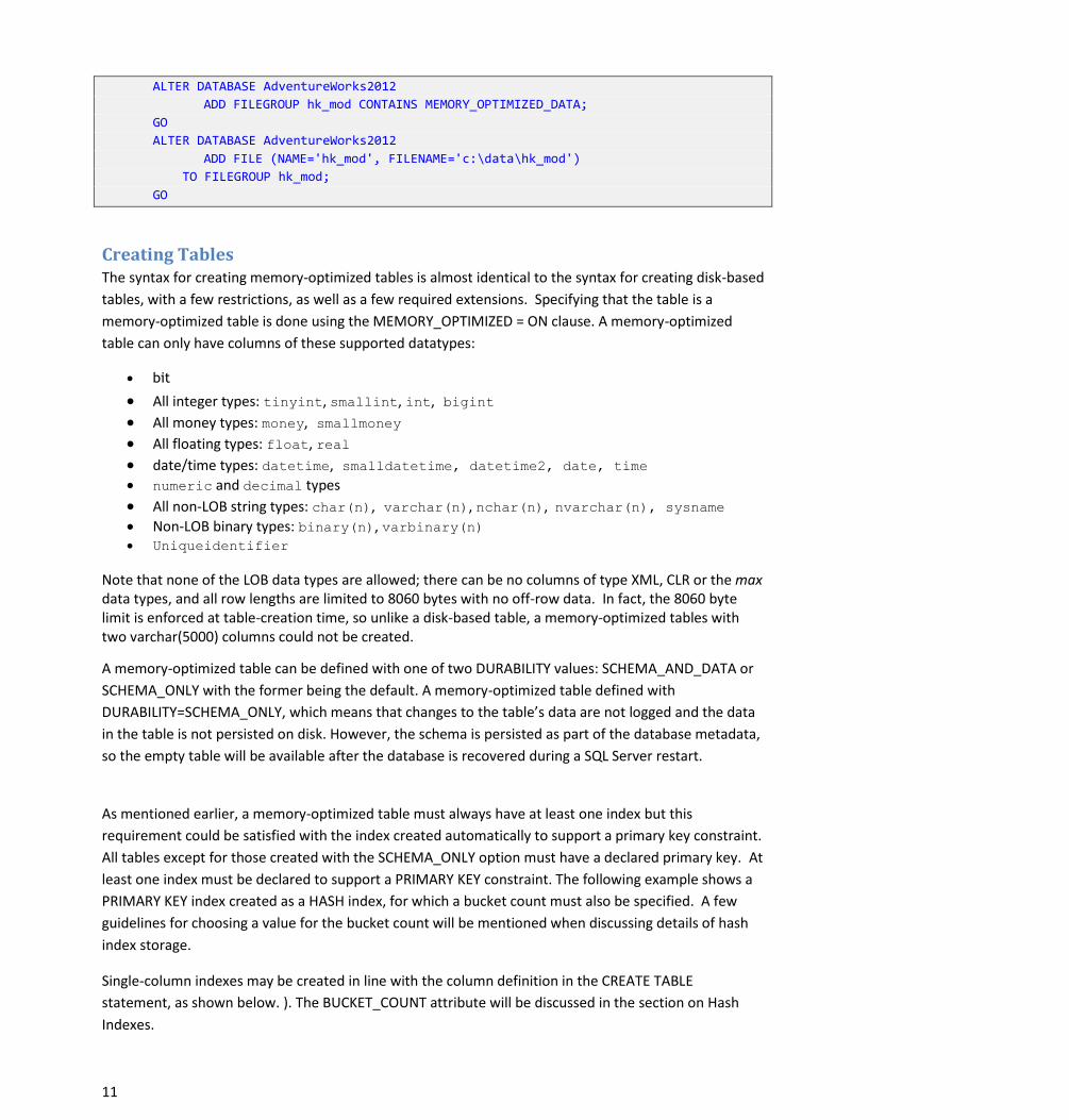
Alternatively, composite indexes may be created after all the columns have been defined, as in the
example below. The example below adds a range index to definition above. Notice the difference in the
specification for the two types of indexes is that one uses the keyword HASH, and the other doesn’t.
Both types of indexes are specified as NONCLUSTERED, but if the word HASH is not used, the index is a
range index.
CREATE TABLE T2 ( [Name] varchar(32) not null PRIMARY KEY NONCLUSTERED HASH WITH (BUCKET_COUNT = 100000), [City] varchar(32) null, [State_Province] varchar(32) null, [LastModified] datetime not null, INDEX T1_ndx_c2c3 NONCLUSTERED ([City],[State_Province]) ) WITH (MEMORY_OPTIMIZED = ON, DURABILITY = SCHEMA_AND_DATA);
When a memory-optimized table is created, the In-Memory OLTP engine will generate and compile DML
routines just for accessing that table, and load the routines as DLLs. SQL Server itself does not perform
the actual data manipulation (record cracking) on memory-optimized tables, instead it calls the
appropriate DLL for the required operation when a memory-optimized table is accessed.
There are only a few limitations when creating memory-optimized tables, in addition to the data type
limitations already listed.
No DML triggers
No FOREIGN KEY or CHECK constraints
No IDENTITY columns
No UNIQUE indexes other than for the PRIMARY KEY
A maximum of 8 indexes, including the index supporting the PRIMARY KEY
In addition, no schema changes are allowed once a table is created. Instead of using ALTER TABLE, you
will need to drop and recreate the table. In addition, there are no specific index DDL commands (i.e.
CREATE INDEX, ALTER INDEX, DROP INDEX). Indexes are always created at as part of the table creation.
Row and Index Storage In-Memory OLTP memory-optimized tables and their indexes are stored very differently than disk-based
tables. Memory-optimized tables are not stored on pages like disk-based tables, nor is space allocated
from extents, and this is due to the design principle of optimizing for byte-addressable memory instead
of block-addressable disk.

13
Rows Rows are allocated from structures called heaps, which are different than the type of heaps SQL Server
has supported for disk-based tables. Rows for a single table are not necessarily stored near other rows
from the same table and the only way SQL Server knows what rows belong to the same table is because
they are all connected using the tables’ indexes. This is why memory-optimized tables have the
requirement that there must be at least one index created on them. It is the index that provides
structure for the tables.
The rows themselves have a structure very different than the row structures used for disk-based tables.
Each row consists of a header and a payload containing the row attributes. Figure 2 shows this
structure, as well as expanding on the content of the header area.
Figure 2 The structure of a row in a memory-optimized table
Row header
The header contains two 8-byte fields holding In-Memory OLTP timestamps: a Begin-Ts and an End-Ts.
Every database that supports memory-optimized tables manages two internal counters that are used to
generate these timestamps.
The Transaction-ID counter is a global, unique value that is reset when the SQL Server instance is
restarted. It is incremented every time a new transaction starts.
The Global Transaction Timestamp is also global and unique, but is not reset on a restart. This
value is incremented each time a transaction ends and begins validation processing. The new
value is then the timestamp for the current transaction. The Global Transaction Timestamp
Row header Payload
Begin Ts End Ts StmtId IdxLinkCount
8 bytes 8 bytes 4 bytes 2 bytes
8 bytes * (Number of indexes)

14
value is initialized during recovery with the highest transaction timestamp found among the
recovered records. (We’ll see more about recovery later in this paper.)
The value of Begin-Ts is the timestamp of the transaction that inserted the row, and the End-Ts value is
the timestamp for the transaction that deleted the row. A special value (referred to as ‘infinity’) is used
as the End-Ts value for rows that have not been deleted. However, when a row is first inserted, before
the insert transaction is completed, the transaction’s timestamp is not known so the global
Transaction_ID value is used for Begin-Ts until the transaction commits. Similarly, for a delete operation,
the transaction timestamp is not known, so the End-Ts value for the deleted rows uses the global
Transaction_ID value, which is replaced once the real Transaction Timestamp is known. As we’ll see
when discussing data operations, the Begin-Ts and End-Ts values determine which other transactions
will be able to see this row.
The header also contains a four-byte statement ID value. Every statement within a transaction has a
unique StmtId value, and when a row is created it stores the StmtId for the statement that created the
row. If the same row is then accessed again by the same statement, it can be skipped.
Finally, the header contains a two-byte value (idxLinkCount) which is really a reference count indicating
how many indexes reference this row. Following the idxLinkCount value is a set of index pointers, which
will be described in the next section. The number of pointers is equal to the number of indexes. The
reference value of 1 that a row starts with is needed so the row can be referenced by the garbage
collection (GC) mechanism even if the row is no longer connected to any indexes. The GC is considered
the ‘owner’ of the initial reference.
As mentioned, there is a pointer for each index on the table, and it is these pointers plus the index data
structures that connect the rows together. There are no other structures for combining rows into a table
other than to link them together with the index pointers. This creates the requirement that all memory-
optimized tables must have at least one index on them. Also, since the number of pointers is part of the
row structure, and rows are never modified, all indexes must be defined at the time your memory-
optimized table is created.
Payload area
The payload is the row itself, containing the key columns plus all the other columns in the row. (So this
means that all indexes on a memory-optimized table are actually covering indexes.) The payload format
can vary depending on the table. As mentioned earlier in the section on creating tables, the In-Memory
OLTP compiler generates the DLLs for table operations, and as long as it knows the payload format used
when inserting rows into a table, it can also generate the appropriate commands for all row operations.
Indexes On Memory-Optimized Tables All memory-optimized tables must have at least one index, because it is the indexes that connect the
rows together. As mentioned earlier, data rows are not stored on pages, so there is no collection of
pages or extents, no partitions or allocation units that can be referenced to get all the pages for a table.
There is some concept of index pages for one of the types of indexes, but they are stored differently
than indexes for disk-based tables.
In-Memory OLTP indexes, and changes made to them during data manipulation, are never written to
disk. Only the data rows, and changes to the data, are written to the transaction log. All indexes on

15
memory-optimized tables are created based on the index definitions during database recovery. We’ll
cover details of in the Checkpoint and Recovery section below.
Hash Indexes
A hash index consists of an array of pointers, and each element of the array is called a hash bucket. The
index key column in each row has a hash function applied to it, and the result of the function determines
which bucket is used for that row. All key values that hash to the same value (have the same result from
the hash function) are accessed from the same pointer in the hash index and are linked together in a
chain. When a row is added to the table, the hash function is applied to the index key value in the row.
If there is duplication of key values, the duplicates will always generate the same function result and
thus will always be in the same chain.
Figure 3 shows one row in a hash index on a name column. For this example, assume there is a very
simple hash function that results in a value equal to the length of the string in the index key column. The
first value of ‘Jane’ will then hash to 4, which is the first bucket in the hash index so far. (Note that the
real hash function is much more random and unpredictable, but I am using the length example to make
it easier to illustrate.) You can see the pointer from the 4 entry in the hash table to the row with Jane.
That row doesn’t point to any other rows, so the index pointer in the record is NULL.
Figure 3 A hash index with a single row
In Figure 4, a row with a name value of Greg has been added to the table. Since we’ll assume that Greg
also maps to 4, it hashes to the same bucket as Jane, and the row is linked into the same chain as the
row for Jane. The Greg row has a pointer to the Jane row.

16
Figure 4 A hash index with two rows
A second hash index included in the table definition on the City column creates a second pointer field.
Each row in the table now has two pointers pointing to it, and the ability to point to two more rows, one
for each index. The first pointer in each row points to the next value in the chain for the Name index; the
second pointer points to the next value in the chain for the City index. Figure 5 shows the same hash
index on Name, this time with three rows that hash to 4, and two rows that hash to 5, which uses the
second bucket in the Name index. The second index on the City column uses three buckets. The bucket
for 6 has three values in the chain, the bucket for 7 has one value in the chain, and the bucket for 8 also
has one value.
Figure 5 Two hash indexes on the same table

17
When a hash index is created, you must specify a number of buckets, as shown in the CREATE TABLE
example above. It is recommended that you choose a number of buckets equal to or greater than the
expected cardinality (the number of unique values) of the index key column so that there will be a
greater likelihood that each bucket will only have rows with a single value in its chain. Be careful not to
choose a number that is too big however, because each bucket uses memory. The number you supply is
rounded up to the next power of two, so a value of 50,000 will be rounded up to 65,536. Having extra
buckets will not improve performance but will simply waste memory and possible reduce the
performance of scans which will have to check each bucket for rows.
When deciding to build a hash index, keep in mind that the hash function actually used is based on ALL
the key columns. This means that if you have a hash index on the columns: lastname, firstname in an
employees table, a row with the values “Harrison” and “Josh” will probably hash to a different bucket
than a row with the values “Harrison” and “John”. A query that just supplies a lastname value, or one
with an inexact firstname value (such as “Jo%”) will not be able to use the index at all.
Range Indexes
If you have no idea of the number of buckets you’ll need for a particular column, or if you know you’ll be
searching your data based on a range of values, you should consider creating a range index instead of a
hash index. Range indexes are implemented using a new data structure called a Bw-tree, originally
envisioned and described by Microsoft Research in 2011. A Bw-tree is a lock- and latch-free variation of
a B-tree.
The general structure of a Bw-tree is similar to SQL Server’s regular B-trees, except that the index pages
are not a fixed size, and once they are built they are unchangeable. Like a regular B-tree page, each
index page contains a set of ordered key values, and for each value there is a corresponding pointer. At
the upper levels of the index, on what are called the internal pages, the pointers point to an index page
at the next level of the tree, and at the leaf level, the pointers point to a data row. Just like for In-
Memory OLTP hash indexes, multiple data rows can be linked together. In the case of range indexes,
rows that have the same value for the index key will be linked.
One big difference between Bw-trees and SQL Server’s B-trees is that a page pointer is a logical page ID
(PID), instead of a physical page number. The PID indicates a position in a mapping table, which
connects each PID with a physical memory address. Index pages are never updated; instead, they are
replaced with a new page and the mapping table is updated so that the same PID indicates a new
physical memory address.
Figure 6 shows the general structure of Bw-tree, plus the Page Mapping Table.
18
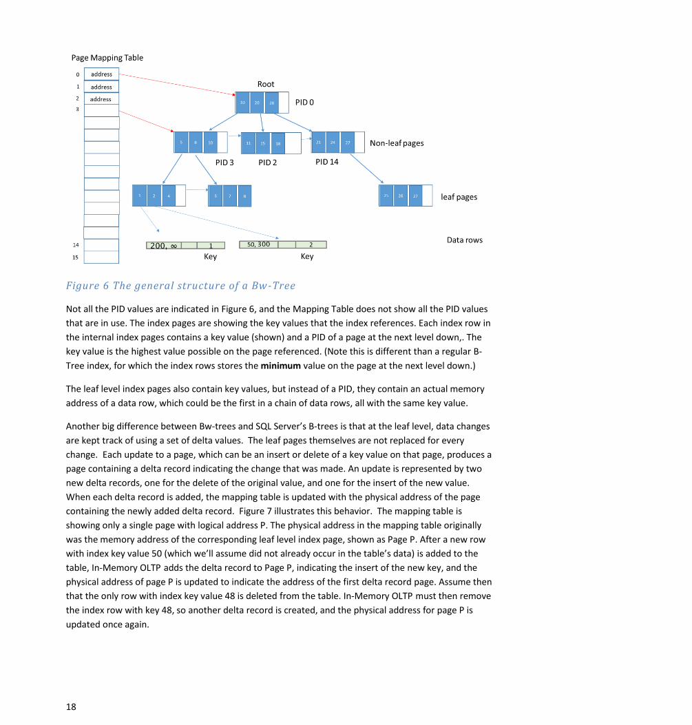
Figure 6 The general structure of a Bw-Tree
Not all the PID values are indicated in Figure 6, and the Mapping Table does not show all the PID values
that are in use. The index pages are showing the key values that the index references. Each index row in
the internal index pages contains a key value (shown) and a PID of a page at the next level down,. The
key value is the highest value possible on the page referenced. (Note this is different than a regular B-
Tree index, for which the index rows stores the minimum value on the page at the next level down.)
The leaf level index pages also contain key values, but instead of a PID, they contain an actual memory
address of a data row, which could be the first in a chain of data rows, all with the same key value.
Another big difference between Bw-trees and SQL Server’s B-trees is that at the leaf level, data changes
are kept track of using a set of delta values. The leaf pages themselves are not replaced for every
change. Each update to a page, which can be an insert or delete of a key value on that page, produces a
page containing a delta record indicating the change that was made. An update is represented by two
new delta records, one for the delete of the original value, and one for the insert of the new value.
When each delta record is added, the mapping table is updated with the physical address of the page
containing the newly added delta record. Figure 7 illustrates this behavior. The mapping table is
showing only a single page with logical address P. The physical address in the mapping table originally
was the memory address of the corresponding leaf level index page, shown as Page P. After a new row
with index key value 50 (which we’ll assume did not already occur in the table’s data) is added to the
table, In-Memory OLTP adds the delta record to Page P, indicating the insert of the new key, and the
physical address of page P is updated to indicate the address of the first delta record page. Assume then
that the only row with index key value 48 is deleted from the table. In-Memory OLTP must then remove
the index row with key 48, so another delta record is created, and the physical address for page P is
updated once again.

19
Figure 7 Delta records linked to a leaf level index page
Index page structures
In-Memory OLTP range index pages are not a fixed size as they are for indexes on disk-based tables,
although the maximum index page size is still 8 KB.
Range index pages for memory-optimized tables all have a header area which contains the following
information:
PID - the pointer into the mapping table
Page Type - leaf, internal, delta or special
Right PID - the PID of the page to the right of the current page
Height – the vertical distance from the current page to the leaf
Page statistics – the count of delta records plus the count of records on the page
Max Key – the upper limit of values on the page
In addition, both leaf and internal pages contains two or three fixed length arrays:
Values – this is really a pointer array. Each entry in the array is 8 bytes long. For internal pages
the entry contains PID of a page at the next level and for a leaf page, the entry contains the
memory address for the first row in a chain of rows having equal key values. (Note that
technically, the PID could be stored in 4 bytes, but to allow the same values structure to be used
for all index pages, the array allows 8 bytes per entry.)
Offsets – this array exists only for pages of indexes with variable length keys. Each entry is 2
bytes and contains the offset where the corresponding key starts in the key array on the page.
Keys – this is the array of key values. If the current page is an internal page, the key represents
the first value on the page referenced by the PID. If the current page is a leaf page, the key is the
value in the chain of rows.
The smallest pages are typically the delta pages, which have a header which contains most of the same
information as in an internal or leaf page. However delta page headers don’t have the arrays described
for leaf or internal pages. A delta page only contains an operation code (insert or delete) and a value,
which is the memory address of the first row in a chain of records. Finally, the delta page will also

20
contain the key value for the current delta operation. In effect you can think of a delta page as being a
mini-index page holding a single element whereas the regular index pages store an array of N elements.
Bw-tree internal reorganization operations
There are three different operations that can be required for managing the structure of a Bw-tree:
consolidation, split and merge. For all of these operations, no changes are made to existing index pages.
Changes may be made to the mapping table to update the physical address corresponding to a PID
value. If an index page needs to add a new row (or have a row removed) a whole new page is created
and the PID values are updated in the Mapping Table.
Consolidation of delta records
A long chain of delta records can eventually degrade search performance, if SQL Server has to consider
the changes in the delta records along with the contents of the index pages when it’s searching through
an index. If In-Memory OLTP attempts to add a new delta record to a chain that already has 16
elements, the changes in the delta records will be consolidated into the referenced index page, and the
page will then be rebuilt, including the changes indicated by the new delta record that triggered the
consolidation. The newly rebuilt page will have the same PID but a new memory address. The old pages
(index page plus delta pages) will be marked for garbage collection.
Splitting of a full index page
An index page in BW-Tree grows on as-needed basis starting from storing a single row to storing a
maximum of 8K bytes. Once the index page grows to 8K bytes, a new insert of a single row will cause the
index page to split. For an internal page, this means when there is no more room to add another key
value and pointer, and for a leaf page, it means that the row would be too big to fit on the page once all
the delta records are incorporated. The statistics information in the page header for a leaf page keeps
track of how much space would be required to consolidate the delta records, and that information is
adjusted as each new delta record is added. A split operation is done in two atomic steps as described
here. Assume Ps is the page to be split into pages P1 and P2 and the Pp is the parent page, with a row that
points to Ps .
Step1: allocate two new pages P1 and P2 and split the rows from page Ps onto these pages, including
the newly inserted row. A new slot in Page Mapping table is used to store the physical address of
page P2. These pages, P1 and P2 are not accessible to any concurrent operations yet. In addition, the
‘logical’ pointer from P1to P2 is set. Once this is done, in one atomic operation update the
PageMapping Table to change the pointer to point to P1 instead of Ps. After this operation, there is
no pointer to page Ps.
Step2: after step-1, the parent page Pp points to P1 but there is no direct pointer from a parent page
to page P2. Page P2 is only reachable via page P1. To create a pointer from a parent page to page P2,
allocate a new parent page Pnp, copy all the rows from page Pp and add a new row to point to page
P2. Once this is done, in one atomic operation, update the Page Mapping Table to change the
pointer from Pp to Pnp
Merging of adjacent index pages
When a delete operation leaves an index page P less than 10% of the maximum page size (currently 8K),
or with a single row on it, page P will be merged with its neighboring page. Like splitting, this is also a
multi-step operation. For this example, we’ll assume we’ll be merging a page with its left neighbor, that
is, one with smaller values. When a row is deleted from page P, a delta record for the delete is added as
21
usual. Additionally, a check is made to determine if the page P qualifies for Merge (i.e. the remaining
space after deleting the row will be less than 10% of maximum page size). If it does qualify, the merge is
performed in three atomic steps as described below. For this example, assume page Pp is the parent
page with a row that points to page P. Page Pln represents the left neighbor, and we’ll assume its
maximum key value is 5. The means the row in the parent Page Pp that points to page Pln contains the
value 5. We are deleting a row with key value 10 on page P. After the delete, there will only be one row
left on page P, with the key value 9.
Step1: A delta page DP10 representing key value 10 is created and its pointer is set to point to P. Additionally a special ‘merge-delta page’ DPm is created it is linked to point to DP10. Note, at this stage, both pages DP10 and DPm are not visible to any concurrent transactions. In one atomic step, the pointer to page P in the Page Mapping Table is updated to point to DPm. After this step, the entry for key value 10 in parent page Pp now points to DPm.
Step2: In this step, the row representing key value 5 in the page Pp is removed and the entry for key value 10 is updated to point to page Pln. To do this, a new non-leaf page Pp2 is allocated and all the rows from Pp are copied except for the row representing key value 5; then the row for key value 10 is updated to point to page Pln. Once this is done, in one atomic step, the page mapping table entry pointing to page Pp is updated to point to page Pp2. Page Pp is no longer reachable.
Step3: In this step the leaf pages P and Pln are merged and the delta pages are removed. To do this, a new page Pnew is allocated and the rows from P and Pln are merged, and the delta page changes are included in the new Pnew. Now, in 1 atomic operation, the page mapping table entry pointing to page Pln is updated to point to page Pnew.
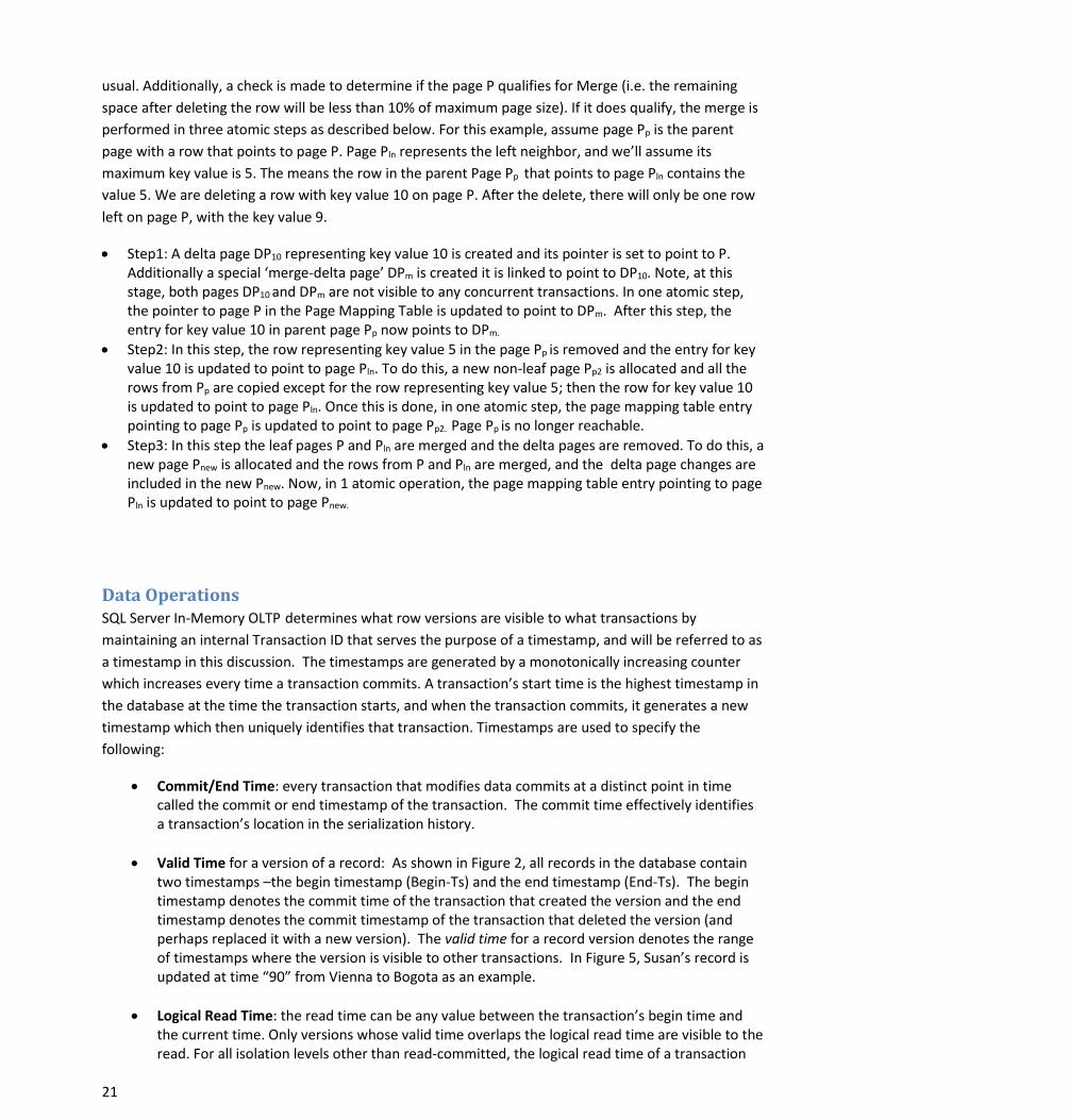
Data Operations SQL Server In-Memory OLTP determines what row versions are visible to what transactions by
maintaining an internal Transaction ID that serves the purpose of a timestamp, and will be referred to as
a timestamp in this discussion. The timestamps are generated by a monotonically increasing counter
which increases every time a transaction commits. A transaction’s start time is the highest timestamp in
the database at the time the transaction starts, and when the transaction commits, it generates a new
timestamp which then uniquely identifies that transaction. Timestamps are used to specify the
following:
Commit/End Time: every transaction that modifies data commits at a distinct point in time called the commit or end timestamp of the transaction. The commit time effectively identifies a transaction’s location in the serialization history.
Valid Time for a version of a record: As shown in Figure 2, all records in the database contain two timestamps –the begin timestamp (Begin-Ts) and the end timestamp (End-Ts). The begin timestamp denotes the commit time of the transaction that created the version and the end timestamp denotes the commit timestamp of the transaction that deleted the version (and perhaps replaced it with a new version). The valid time for a record version denotes the range of timestamps where the version is visible to other transactions. In Figure 5, Susan’s record is updated at time “90” from Vienna to Bogota as an example.
Logical Read Time: the read time can be any value between the transaction’s begin time and the current time. Only versions whose valid time overlaps the logical read time are visible to the read. For all isolation levels other than read-committed, the logical read time of a transaction

22
corresponds to the start of the transaction. For read-committed it corresponds to the start of a statement within the transaction.
The notion of version visibility is fundamental to proper concurrency control in In-Memory OLTP. A
transaction executing with logical read time RT must only see versions whose begin timestamp is less
than RT and whose end timestamp is greater than RT.
Isolation Levels Allowed with Memory-Optimized Tables
Data operations on memory-optimized tables always use optimistic multi version concurrency control
(MVCC). Optimistic data access does not use locking or latching to provide transaction isolation. We’ll
look at the details of how this lock and latch free behavior is managed, as well as details on the reasons
for the allowed transaction isolation levels in a later section. In this section, we’ll only be discussing the
details of transaction isolation level necessary to understand the basics of data access and modification
operations.
The following isolation levels are supported for transactions accessing memory-optimized tables.
SNAPSHOT REPEATABLE READ SERIALIZABLE
The transaction isolation level can be specified as part of the ATOMIC block of a natively compiled stored procedure. Alternatively, when accessing memory-optimized tables from interpreted Transact-SQL, the isolation level can be specified using table-level hints or a new database option called MEMORY_OPTIMIZED_ELEVATE_TO_SNAPSHOT. This option will be discussed later, after we have looked at isolation levels for accessing memory-optimized tables.
Specification of the transaction isolation level is required with natively compiled stored procedures. Specification of the isolation level in table hints is required when accessing memory-optimized tables from user transactions in interpreted Transact-SQL.
The isolation level READ COMMITTED is supported for memory optimized tables with autocommit (single statement) transactions. It is not supported with explicit or implicit user transactions. (Implicit transactions are those invoked under the session option IMPLICIT_TRANSACTIONS. In this mode, behavior is the same as for an explicit transaction, but no BEGIN TRANSACTION statement is required. Any DML statement will start a transaction, and the transaction must be explicitly either committed or rolled back. Only the BEGIN TRANSACTION is implicit.) Isolation level READ_COMMITTED_SNAPSHOT is supported for memory-optimized tables with autocommit transactions and only if the query does not access any disk-based tables. In addition, transactions that are started using interpreted Transact-SQL with SNAPSHOT isolation cannot access memory-optimized tables. Transactions that are started using interpreted Transact-SQL with either REPEATABLE READ or SERIALIZABLE isolation must access memory-optimized tables using SNAPSHOT isolation.
Given the in-memory structures for rows previously described, let’s now look at how DML operations
are performed by walking through an example. We will indicate rows by listing the contents in order, in
angle brackets. Assume we have a transaction TX1 with transaction ID 100 running at SERIALIZABLE
isolation level that starts at timestamp 240 and performs two operations:
DELETE the row <Greg , Lisbon>
23
UPDATE <Jane, Helsinki> to <Jane, Perth>
Concurrently, two other transactions will read the rows. TX2 is an auto-commit, single statement
SELECT that runs at timestamp 243. TX3 is an explicit transaction that reads a row and then updates
another row based on the value it read in the SELECT; it has a timestamp of 246.
First we’ll look at the data modification transaction. The transaction begins by obtaining a begin
timestamp that indicates when it began relative to the serialization order of the database. In our
example, that timestamp is 240.
While it is operating, transaction TX1 will only be able to access records that have a begin timestamp
less than or equal to 240 and an end timestamp greater than 240.
Deleting
Transaction TX1 first locates <Greg, Lisbon> via one of the indexes. To delete the row, the end
timestamp on the row is set to 100 with an extra flag bit indicating that the value is a transaction ID.
Any other transaction that now attempts to access the row finds that the end timestamp contains a
transaction ID (100) which indicates that the row may have been deleted. It then locates TX1 in the
transaction map and checks if transaction TX1 is still active to determine if the deletion of <Greg ,
Lisbon> has been completed or not.
Updating and Inserting
Next the update of <Jane, Helsinki> is performed by breaking the operation into two separate
operations: DELETE the entire original row, and INSERT a complete new row. This begins by
constructing the new row <Jane, Perth> with begin timestamp 100 containing a flag bit indicating that it
is a transaction ID, and then setting the end timestamp to ∞ (infinity). Any other transaction that
attempts to access the row will need to determine if transaction TX1 is still active to decide whether it
can see <Jane, Perth> or not. Then <Jane, Perth> is inserted by linking it into both indexes. Next <Jane,
Helsinki> is deleted just as described for the DELETE operation in the preceding paragraph. Any other
transaction that attempts to update or delete <Jane, Helsinki> will notice that the end timestamp does
not contain infinity but a transaction ID, conclude that there is write-write conflict, and immediately
abort.
At this point transaction TX1 has completed its operations but not yet committed. Commit processing
begins by obtaining an end timestamp for the transaction. This end timestamp, assume 250 for this
example, identifies the point in the serialization order of the database where this transaction’s updates
have logically all occurred. In obtaining this end timestamp, the transaction enters a state called
validation where it performs checks to ensure it that there are no violations of the current isolation
level. If the validation fails, the transaction is aborted. More details about validation are covered
shortly. SQL Server will also write to the transaction log at the end of the validation phase.
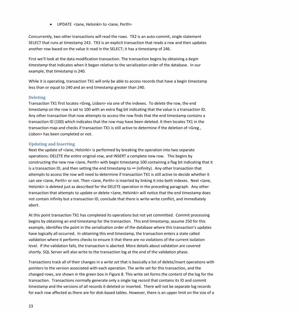
Transactions track all of their changes in a write set that is basically a list of delete/insert operations with
pointers to the version associated with each operation. The write set for this transaction, and the
changed rows, are shown in the green box in Figure 8. This write set forms the content of the log for the
transaction. Transactions normally generate only a single log record that contains its ID and commit
timestamp and the versions of all records it deleted or inserted. There will not be separate log records
for each row affected as there are for disk-based tables. However, there is an upper limit on the size of a

24
log record, and if a transaction on memory-optimized tables exceeds the limit, there can be multiple log
records generated. Once the log record has been hardened to storage the state of the transaction is
changed to committed and post-processing is started.
Post-processing involves iterating over the write set and processing each entry as follows:
For a DELETE operation, set the row’s end timestamp to the end timestamp of the transaction (in this case 250) and clear the type flag on the row’s end timestamp field.
For an INSERT operation, set the affected row’s begin timestamp to the end timestamp of the transaction (in this case 250) and clear the type flag on the row’s begin timestamp field
The actual unlinking and deletion of old row versions is handled by the garbage collection system, which
will be discussed below.
Figure 8 Transactional Modifications on a table
Reading
Now let’s look at the read transactions, TX2 and TX3, which will be processed concurrently with TX1.
Remember that TX1 is deleting the row <Greg , Lisbon> and updating <Jane, Helsinki> to <Jane, Perth> .
TX2 is an autocommit transaction that reads the entire table:
SELECT Name, City
FROM T1
25
TX2’s session is running in the default isolation level READ COMMITTED, but as described above,
because no hints are specified, and T1 is memory-optimized table, the data will be accessed using
SNAPSHOT isolation. Because TX2 runs at timestamp 243, it will be able to read rows that existed at that
time. It will not be able to access <Greg, Beijing> because that row no longer is valid at timestamp 243.
The row <Greg, Lisbon> will be deleted as of timestamp 250, but it is valid between timestamps 200 and
250, so transaction TX2 can read it. TX2 will also read the <Susan, Bogota> row and the <Jane, Helsinki>
row.
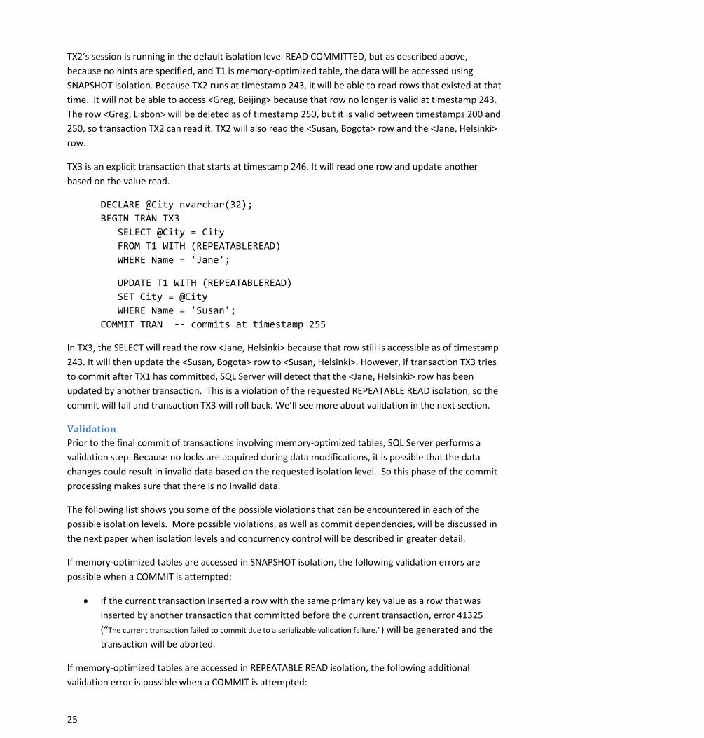
TX3 is an explicit transaction that starts at timestamp 246. It will read one row and update another
based on the value read.
DECLARE @City nvarchar(32);
BEGIN TRAN TX3
SELECT @City = City
FROM T1 WITH (REPEATABLEREAD)
WHERE Name = 'Jane';
UPDATE T1 WITH (REPEATABLEREAD)
SET City = @City
WHERE Name = 'Susan';
COMMIT TRAN -- commits at timestamp 255
In TX3, the SELECT will read the row <Jane, Helsinki> because that row still is accessible as of timestamp
243. It will then update the <Susan, Bogota> row to <Susan, Helsinki>. However, if transaction TX3 tries
to commit after TX1 has committed, SQL Server will detect that the <Jane, Helsinki> row has been
updated by another transaction. This is a violation of the requested REPEATABLE READ isolation, so the
commit will fail and transaction TX3 will roll back. We’ll see more about validation in the next section.
Validation
Prior to the final commit of transactions involving memory-optimized tables, SQL Server performs a
validation step. Because no locks are acquired during data modifications, it is possible that the data
changes could result in invalid data based on the requested isolation level. So this phase of the commit
processing makes sure that there is no invalid data.
The following list shows you some of the possible violations that can be encountered in each of the
possible isolation levels. More possible violations, as well as commit dependencies, will be discussed in
the next paper when isolation levels and concurrency control will be described in greater detail.
If memory-optimized tables are accessed in SNAPSHOT isolation, the following validation errors are
possible when a COMMIT is attempted:
If the current transaction inserted a row with the same primary key value as a row that was
inserted by another transaction that committed before the current transaction, error 41325
(“The current transaction failed to commit due to a serializable validation failure.”) will be generated and the
transaction will be aborted.
If memory-optimized tables are accessed in REPEATABLE READ isolation, the following additional
validation error is possible when a COMMIT is attempted:

26
If the current transaction has read any row that was then updated by another
transaction that committed before the current transaction, error 41305 (“The
current transaction failed to commit due to a repeatable read validation failure.”) will be
generated and the transaction will be aborted.
If memory-optimized tables are accessed in SERIALIZABLE isolation, the following additional validation
errors are possible when a COMMIT is attempted:
If the current transaction fails to read any valid rows that meet the specified filter conditions, or
encounters phantoms rows inserted by other transactions that meet the specified filter
conditions, the commit will fail. The transaction needs to be executed as if there are no
concurrent transactions. All actions logically happen at a single serialization point. If any of these
guarantees are violated, error 41325 is generated and the transaction will be aborted.
T-SQL Support
Memory-optimized tables can be accessed in two different ways: either through interop, using
interpreted Transact-SQL, or through natively compiled stored procedures.
Interpreted Transact-SQL
When using the interop capability, you will have access to virtually the full Transact-SQL surface area
when working with your memory-optimized tables, but you should not expect the same performance as
when you access memory-optimized tables using natively compiled stored procedures. Interop is the
appropriate choice when running ad hoc queries, or to use while migrating your applications to In-
Memory OLTP, as a step in the migration process, before migrating the most performance critical
procedures. Interpreted Transact-SQL should also be used when you need to access both memory-
optimized tables and disk-based tables.
The only Transact-SQL features not supported when accessing memory-optimized tables using interop
are the following:
TRUNCATE TABLE
MERGE (when a memory-optimized table is the target)
Dynamic and keyset cursors (these are automatically degraded to static cursors)
Cross-database queries
Cross-database transactions
Linked servers
Locking hints: TABLOCK, XLOCK, PAGLOCK, , etc. (NOLOCK is supported, but is quietly ignored.)
Isolation level hints READUNCOMMITTED, READCOMMITTED and READCOMMITTEDLOCK
Memory-optimized table types and table variables are not supported in CTP1 only
T-SQL in Natively Compiled Procedures
Natively compiled stored procedures allow you to execute Transact-SQL in the fastest way, which
includes accessing data in memory-optimized tables. There are however, many more limitations on the
Transact-SQL that is allowed in these procedures. There are also limitations on the data types and

27
collations that can be accessed and processed in natively compiled procedures. Please refer to the
documentation for the full list of supported Transact-SQL statements, data types and operators that are
allowed. In addition, disk-based tables are not allowed to be accessed at all inside natively compiled
stored procedures.
The reason for the restrictions is due to the fact that internally, a separate function must be created for
each operation on each table. The interface will be expanded in subsequent versions.
Garbage Collection of Rows in Memory
Because In-Memory OLTP is a multi-versioning system, your DELETE and UPDATE operations (as well as
aborted INSERT operations) will generate row versions that will eventually become stale, which means
they will no longer be visible to any transaction. These unneeded versions will slow down scans of index
structures and create unused memory that needs to be reclaimed.
The garbage collection process for stale versions in your memory-optimized tables is analogous to the
version store cleanup that SQL Server performs for disk-based tables using one of the snapshot-based
isolation levels. A big difference though is that the cleanup is not done in tempdb, but in the in-memory
table structures themselves.
To determine which rows can be safely deleted, the system keeps track of the timestamp of the oldest
active transaction running in the system, and uses this value to determine which rows are still
potentially needed. Any rows that are not valid as of this point in time (that is, their end-timestamp is
earlier than this time) are considered stale. Stale rows can be removed and their memory can be
released back to the system.
The garbage collection system is designed to be non-blocking, cooperative, efficient, responsive and
scalable. Of particular interest is the ‘cooperative’ attribute. Although there is a dedicated system thread
for the garbage collection process, user threads actually do most of the work. If a user thread is scanning
an index (and all index access on memory-optimized tables is considered to be scanning) and it comes
across a stale row version, it will unlink that version from the current chain and adjust the pointers. It
will also decrement the reference count in the row header area. In addition, when a user thread
completes a transaction, it then adds information about the transaction to a queue of transactions to be
processed by the garbage collection process. Finally, it picks up one or more work items from a queue
created by the garbage collection thread, and frees the memory used by the rows making up the work
item.
The garbage collection thread goes through queue of completed transactions about once a minute, but
the system can adjust the frequency internally based on the number of completed transactions waiting
to be processed. From each transaction, it determines which rows are stale, and builds work items
made up of a set of rows that are ready for removal. In CTP2, the number of rows in a set is 16, but that
number is subject to change in future versions. These work items are distributed across multiple
queues, one for each CPU used by SQL Server. Normally, the work of actually removing the rows from
memory is left to the user threads which process these work items from the queues, but if there is little
user activity, the garbage collection thread itself can remove rows to reclaim system memory.
The DVM sys.dm_db_xtp_index_stats has a row for each index on each memory-optimized table, and
the column rows_expired indicates how many rows have been detected as being stale during scans of
that index. There is also a column called rows_expired_removed that indicates how many rows have

28
been unlinked from that index. As mentioned above, once rows have been unlinked from all indexes on
a table, it can be removed by the garbage collection thread. So you will not see the
rows_expired_removed value going up until the rows_expired counters have been incremented for every
index on a memory-optimized table.
The following query allows you to observe these values. It joins the sys.dm_db_xtp_index_stats DMV
with the sys.indexes catalog view to be able to return the name of the index.
SELECT name AS 'index_name', s.index_id, scans_started, rows_returned,
rows_expired, rows_expired_removed
FROM sys.dm_db_xtp_index_stats s JOIN sys.indexes i
ON s.object_id=i.object_id and s.index_id=i.index_id
WHERE object_id('<memory-optimized table name>') = s.object_id;
GO
Transaction Isolation and Concurrency Management As mentioned above, all access of data in memory-optimized tables is done using completely optimistic
concurrency control, but multiple transaction isolation levels are still allowed. However, what isolation
levels are allowed in what situations might seem a little confusing and non-intuitive. The isolation levels
we are concerned about are the ones involving a cross container transaction, which means any
interpreted query that references memory-optimized tables whether executed from an explicit or
implicit transaction or in auto-commit mode. The isolation levels that can be used with your memory-
optimized tables in a cross-container transaction depend on what isolation level the transaction has
defined for the SQL Server transaction. Most of the restrictions have to do with the fact that operations
on disk-based tables and operations on memory-optimized tables each have their own transaction
sequence number, even if they are accessed in the same Transact-SQL transaction. You can think of this
behavior as having two sub-transactions within the larger transaction: one sub-transaction is for the
disk-based tables and one is for the memory-optimized tables.
First, let me give you a little background on isolation levels in general. This will not be a complete
discussion of isolation levels, which is beyond the scope of this paper. Isolation levels can be defined in
terms of the consistency properties that are guaranteed. The most important properties are the
following:
1. Read Stability. If T reads some version V1 of a record during its processing, we must guarantee that V1 is still the version visible to T as of the end of the transaction, that is, V1 has not been replaced by another committed version V2. This can be implemented either by read locking V1 to prevent updates or by validating that V1 has not been updated before commit.
2. Phantom Avoidance. We must be able to guarantee that a transaction T’s scans would not return additional new versions added between the time T starts and the time T commits. This can be implemented in two ways: by locking the scanned part of an index/table or by rescanning to check for new versions before commit.
Then we can define the transaction isolation level based on these properties. The first one listed
(SNAPSHOT) does not mention these properties, but the second two do.
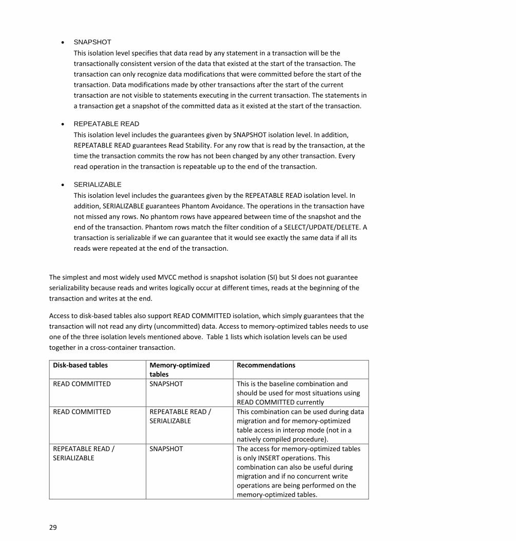
29
SNAPSHOT
This isolation level specifies that data read by any statement in a transaction will be the
transactionally consistent version of the data that existed at the start of the transaction. The
transaction can only recognize data modifications that were committed before the start of the
transaction. Data modifications made by other transactions after the start of the current
transaction are not visible to statements executing in the current transaction. The statements in
a transaction get a snapshot of the committed data as it existed at the start of the transaction.
REPEATABLE READ
This isolation level includes the guarantees given by SNAPSHOT isolation level. In addition,
REPEATABLE READ guarantees Read Stability. For any row that is read by the transaction, at the
time the transaction commits the row has not been changed by any other transaction. Every
read operation in the transaction is repeatable up to the end of the transaction.
SERIALIZABLE
This isolation level includes the guarantees given by the REPEATABLE READ isolation level. In
addition, SERIALIZABLE guarantees Phantom Avoidance. The operations in the transaction have
not missed any rows. No phantom rows have appeared between time of the snapshot and the
end of the transaction. Phantom rows match the filter condition of a SELECT/UPDATE/DELETE. A
transaction is serializable if we can guarantee that it would see exactly the same data if all its
reads were repeated at the end of the transaction.
The simplest and most widely used MVCC method is snapshot isolation (SI) but SI does not guarantee
serializability because reads and writes logically occur at different times, reads at the beginning of the
transaction and writes at the end.
Access to disk-based tables also support READ COMMITTED isolation, which simply guarantees that the
transaction will not read any dirty (uncommitted) data. Access to memory-optimized tables needs to use
one of the three isolation levels mentioned above. Table 1 lists which isolation levels can be used
together in a cross-container transaction.
Disk-based tables Memory-optimized tables
Recommendations
READ COMMITTED SNAPSHOT This is the baseline combination and should be used for most situations using READ COMMITTED currently
READ COMMITTED REPEATABLE READ / SERIALIZABLE
This combination can be used during data migration and for memory-optimized table access in interop mode (not in a natively compiled procedure).
REPEATABLE READ / SERIALIZABLE
SNAPSHOT The access for memory-optimized tables is only INSERT operations. This combination can also be useful during migration and if no concurrent write operations are being performed on the memory-optimized tables.

30
SNAPSHOT - No memory-optimized table access allowed (see note 1)
REPEATABLE READ / SERIALIZABLE
REPEATABLE READ / SERIALIZABLE
This combination is not allowed (see note 2)
Table 1 Compatible isolation levels in cross-container transactions
Note 1: For SHAPSHOT Isolation, all operations need to see the versions of the data that existed as of
the beginning of the transaction. For SNAPSHOTs, the beginning of the transaction is measured when
the first table is accessed. In a cross-container transaction, however, since the sub-transactions can
each start at a different time, another transaction may have changed data between the start times of
the two sub-transactions. The cross-container transaction then will have no one point in time that the
snapshot is based on.
Note 2: The reason both the sub-transactions (the one on the disk-based tables and the one on the
memory-optimized tables) can’t use REPEATABLE READ or SERIALZABLE is because the two systems
implement the isolation levels in different ways. Imagine the two cross-container transactions in Figure
9.
Time Tx1 (SERIALIZBLE) Tx2 (any isolation level) 1 BEGIN SQL/In-Memory sub-xacts
2 Read RHk1
3 BEGIN SQL/In-Memory sub-transactions
4 Read RSql1 and update to RSql2 5 Read RHk1 and update to RHk2
6 COMMIT
7 Read RSql2
Figure 9 Two concurrent cross-container transactions
Tx1 would read the row from the memory-optimized table first and no locks would be held, so that Tx2
could complete and change the two rows. When Tx1 resumed, when it read the row from the disk-
based table, it would now have a set of values for the two rows that could never have existed if the
transaction were run in isolation (i.e. if the transaction were truly serializable.) So this combination is
not allowed.
For more details on Isolation Levels, please see the following references:
http://en.wikipedia.org/wiki/Isolation_(database_systems)
http://research.microsoft.com/apps/pubs/default.aspx?id=69541
Checkpoint and Recovery SQL Server must ensure transaction durability for memory-optimized tables, so that changes can be
recovered after a failure. In-Memory OLTP achieves this by having both the checkpoint process and the
transaction logging process write to durable storage. Though not covered in this paper, In-Memory OLTP
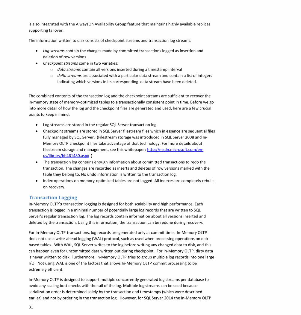
31
is also integrated with the AlwaysOn Availability Group feature that maintains highly available replicas
supporting failover.
The information written to disk consists of checkpoint streams and transaction log streams.
Log streams contain the changes made by committed transactions logged as insertion and
deletion of row versions.
Checkpoint streams come in two varieties:
o data streams contain all versions inserted during a timestamp interval
o delta streams are associated with a particular data stream and contain a list of integers
indicating which versions in its corresponding data stream have been deleted.
The combined contents of the transaction log and the checkpoint streams are sufficient to recover the
in-memory state of memory-optimized tables to a transactionally consistent point in time. Before we go
into more detail of how the log and the checkpoint files are generated and used, here are a few crucial
points to keep in mind:
Log streams are stored in the regular SQL Server transaction log.
Checkpoint streams are stored in SQL Server filestream files which in essence are sequential files
fully managed by SQL Server. (Filestream storage was introduced in SQL Server 2008 and In-
Memory OLTP checkpoint files take advantage of that technology. For more details about
filestream storage and management, see this whitepaper: http://msdn.microsoft.com/en-
us/library/hh461480.aspx )
The transaction log contains enough information about committed transactions to redo the
transaction. The changes are recorded as inserts and deletes of row versions marked with the
table they belong to. No undo information is written to the transaction log.
Index operations on memory-optimized tables are not logged. All indexes are completely rebuilt
on recovery.
Transaction Logging In-Memory OLTP’s transaction logging is designed for both scalability and high performance. Each
transaction is logged in a minimal number of potentially large log records that are written to SQL
Server’s regular transaction log. The log records contain information about all versions inserted and
deleted by the transaction. Using this information, the transaction can be redone during recovery.
For In-Memory OLTP transactions, log records are generated only at commit time. In-Memory OLTP
does not use a write-ahead logging (WAL) protocol, such as used when processing operations on disk-
based tables. With WAL, SQL Server writes to the log before writing any changed data to disk, and this
can happen even for uncommitted data written out during checkpoint. For In-Memory OLTP, dirty data
is never written to disk. Furthermore, In-Memory OLTP tries to group multiple log records into one large
I/O. Not using WAL is one of the factors that allows In-Memory OLTP commit processing to be
extremely efficient.
In-Memory OLTP is designed to support multiple concurrently generated log streams per database to
avoid any scaling bottlenecks with the tail of the log. Multiple log streams can be used because
serialization order is determined solely by the transaction end timestamps (which were described
earlier) and not by ordering in the transaction log. However, for SQL Server 2014 the In-Memory OLTP

32
integration with SQL Server leverages only a single log stream per database (since SQL Server only has
one log file per database). In current testing, this has not been a problem because In-Memory OLTP
generates much less log data and fewer log writes compared with operations on disk-based tables.
The following simple script illustrates the greatly reduced logging for memory-optimized tables. This
script creates a database that can hold memory-optimized tables, and then creates two similar tables.
One is a memory-optimized table, and one is a disk-based table.
USE master
GO
IF EXISTS (SELECT * FROM sys.databases WHERE name='LoggingDemo')
DROP DATABASE LoggingDemo;
GO
CREATE DATABASE LoggingDemo ON
PRIMARY (NAME = [LoggingDemo_data], FILENAME =
'C:\DataHK\LoggingDemo_data.mdf'),
FILEGROUP [LoggingDemo_FG] CONTAINS MEMORY_OPTIMIZED_DATA
(NAME = [LoggingDemo_container1], FILENAME =
'C:\DataHK\StorageDemo_mod_container1')
LOG ON (name = [hktest_log], Filename='C:\DataHK\StorageDemo.ldf',
size=100MB);
GO
USE LoggingDemo
GO
IF EXISTS (SELECT * FROM sys.objects WHERE name='t1_inmem')
DROP TABLE [dbo].[t1_inmem]
GO
-- create a simple memory-optimized table
CREATE TABLE [dbo].[t1_inmem]
( [c1] int NOT NULL,
[c2] char(100) NOT NULL,
CONSTRAINT [pk_index91] PRIMARY KEY NONCLUSTERED HASH ([c1])
WITH(BUCKET_COUNT = 1000000)
) WITH (MEMORY_OPTIMIZED = ON,
DURABILITY = SCHEMA_AND_DATA);
GO
IF EXISTS (SELECT * FROM sys.objects WHERE name='t1_disk')
DROP TABLE [dbo].[t1_disk]
GO
-- create a similar disk-based table
CREATE TABLE [dbo].[t1_disk]
( [c1] int NOT NULL,
[c2] char(100) NOT NULL)
GO
CREATE UNIQUE NONCLUSTERED INDEX t1_disk_index on t1_disk(c1);
GO
Next, populate the disk-based table with 100 rows, and examine the contents of the transaction log
using the undocumented (and unsupported) function fn_dblog().
BEGIN TRAN
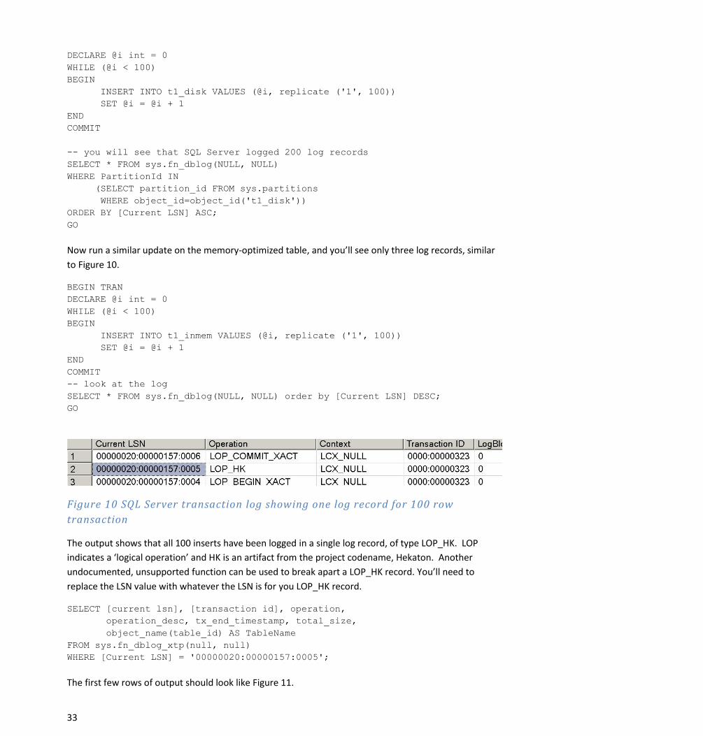
33
DECLARE @i int = 0
WHILE (@i < 100)
BEGIN
INSERT INTO t1_disk VALUES (@i, replicate ('1', 100))
SET @i = @i + 1
END
COMMIT
-- you will see that SQL Server logged 200 log records
SELECT * FROM sys.fn_dblog(NULL, NULL)
WHERE PartitionId IN
(SELECT partition_id FROM sys.partitions
WHERE object_id=object_id('t1_disk'))
ORDER BY [Current LSN] ASC;
GO
Now run a similar update on the memory-optimized table, and you’ll see only three log records, similar
to Figure 10.
BEGIN TRAN
DECLARE @i int = 0
WHILE (@i < 100)
BEGIN
INSERT INTO t1_inmem VALUES (@i, replicate ('1', 100))
SET @i = @i + 1
END
COMMIT
-- look at the log
SELECT * FROM sys.fn_dblog(NULL, NULL) order by [Current LSN] DESC;
GO
Figure 10 SQL Server transaction log showing one log record for 100 row
transaction
The output shows that all 100 inserts have been logged in a single log record, of type LOP_HK. LOP
indicates a ‘logical operation’ and HK is an artifact from the project codename, Hekaton. Another
undocumented, unsupported function can be used to break apart a LOP_HK record. You’ll need to
replace the LSN value with whatever the LSN is for you LOP_HK record.
SELECT [current lsn], [transaction id], operation,
operation_desc, tx_end_timestamp, total_size,
object_name(table_id) AS TableName
FROM sys.fn_dblog_xtp(null, null)
WHERE [Current LSN] = '00000020:00000157:0005';
The first few rows of output should look like Figure 11.

34
Figure 11 Breaking apart the log record for the inserts on the memory -optimized
table shows the individual rows affected
The single log record for the entire transaction on the memory-optimized table, plus the reduced size of
the logged information, helps to make transactions on memory-optimized tables much more efficient.
Checkpoint Just like for operations on disk-based tables, one of the main reasons for checkpoint operations is to
reduce recovery time. The checkpointing process for memory-optimized tables is designed to satisfy two
important requirements.
Continuous checkpointing. Checkpoint related I/O operations occur incrementally and
continuously as transactional activity accumulates. Hyper-active checkpoint schemes (defined as
checkpoint processes which sleep for a while after which they wake up and work as hard as
possible to finish up the accumulated work) can potentially be disruptive to overall system
performance.
Streaming I/O. Checkpointing relies on streaming I/O rather than random I/O for most of its
operations. Even on SSD devices random I/O is slower than sequential I/O and can incur more
CPU overhead due to smaller individual I/O requests.
A checkpoint operation for memory-optimized tables is invoked in four different scenarios:
Manual checkpoint: when an explicit CHECKPOINT command is issued, it initiates checkpoint
operations on both disk-based tables and memory-optimized tables
No transactional activity in disk-based tables or memory-optimized tables. In this case, the In-
Memory OLTP engine performs a time based checkpoint for memory-optimized tables which
adds a 128MB file to storage. Currently, that interval is every 6 hours. The In-Memory OLTP
engine will perform merge operations on these files to make sure the number of files doesn’t just
keep increasing indefinitely. The checkpoint file merging operations will be described below.
There is significant activity on the memory-optimized tables, but no or very little activity on the
disk-based tables, or there is no or little activity in memory-optimized tables but significant activity
in disk-based tables. : The In-Memory OLTP checkpoint is run when the size of the log has
grown by 1 GB since the last checkpoint. In this case, the log generated by memory-optimized
tables will cause the SQL Server engine to actual start the checkpoint as the checkpoint is based
on the log size. So the log truncation point will advance both for SQL Server and In-Memory
OLTP.

35
Checkpoint Files
Checkpoint data is stored in two types of checkpoint files: data files and delta files. A complete
checkpoint consists of multiple data and delta files, plus a checkpoint file inventory that lists the files
comprising the checkpoint. As mentioned earlier,
A data file contains only inserted versions or rows, which, as we saw earlier are generated by both
INSERT and UPDATE operations. Each file covers a specific timestamp range. All versions with a begin
timestamp within the data file’s range are contained in the file. Data files are append-only while they
are open and once they are closed, they are strictly read-only. At recovery time the valid versions in the
data files are reloaded into memory and reindexed.
A delta file stores information about which versions contained in a data file have been subsequently
deleted. There is a 1:1 correspondence between delta files and data files. Delta files are append-only for
the lifetime of the data file they correspond to. At recovery time, the delta file is used as a filter to avoid
reloading deleted versions into memory. Because each data file is paired with exactly one delta file, the
smallest unit of work for recovery is a data/delta file pair. This allows the recovery process to be highly
parallelizable.
A checkpoint file inventory contains references to all the data and delta files that make up a complete
checkpoint. The inventory is written to the transaction log.
A complete checkpoint combined with the tail of the transaction log enables memory-optimized tables
to be recovered. A checkpoint has a timestamp which indicates that the effects of all transactions before
the checkpoint timestamp are recorded in the checkpoint and thus the transaction log is not needed to
recover them.
The Checkpoint Process
A checkpoint task takes a section of the transaction log not covered by a previous checkpoint and
converts all operations on memory-optimized tables contained in that section of the log into one or
more data files and delta files. New row versions are appended to either the most recent data file or
into a new data file and the IDs of deleted versions are appended to the delta files. Once the checkpoint
task finishes processing the log, the checkpoint is completed with the following steps.
1. All buffered writes are flushed to the data and delta files.
2. A checkpoint inventory is constructed that includes descriptors for all files from the previous checkpoint
plus any files added by the current checkpoint. The inventory is hardened to the transaction log.
3. The location of the inventory is stored in the transaction log so that it is available at recovery time.
Merging Checkpoint Files The set of files involved in a checkpoint grows with each check-point. However the active content of a
data file decreases as more and more of its versions are marked as deleted in the corresponding delta
file. Since the recovery process will read the contents of all data and delta files in the checkpoint,
performance of crash recovery degrades as the relevant number of rows in each data file decreases.
The solution to this problem is to merge data files that are adjacent in terms of timestamp ranges, when
their active content (the percentage of undeleted versions in a data file) drops below a threshold.
Merging two data files DF1 and DF2 results in a new data file DF3 covering the combined range of DF1
36
and DF2. All deleted versions identified in the delta files for DF1 and DF2 are removed during the merge.
The delta file for DF3 is empty immediately after the merge, except for deletions that occurred after the
merge operation started.
Merging can also occur when two adjacent data files are each less than 50% full. Data files can end up
only partially full if a manual checkpoint has been run, which closes the currently open checkpoint data
file and starts a new one.
Automatic Merge
To identify files to be merged, a background task periodically looks at all active data/delta file pairs and
identifies zero more sets of files that qualify. Each set can contain two or more data/delta file pairs that
are adjacent to each other such that the resultant set of rows can still fit in a single data file of size
128MB. Figure 12 shows are some examples of files that will be chosen to be merged under the merge
policy.
Adjacent Source Files (%full) Merge Selection
DF0 (30%) DF1 (50%), DF2 (50%), DF3 (90%) (DF1, DF2)
DF0 (30%) DF1 (20%), DF2 (50%), DF3 (10%) (F0, F1, F2). Files are chosen starting from
left
DF0 (80%), DF1 (10%), DF2 (10%), DF3(20%) (DF0, DF1, DF2). Files are chosen starting
from left
Figure 12 Examples of files that can be chosen for file merge operations
It is possible that two adjacent data files are 60% full. They will not be merged and 40% of storage is
unused. So effectively, the total disk storage used for durable memory-optimized tables is larger than
the corresponding memory-optimized size. In the worst case, the size of storage space taken by durable
tables could be two times larger than the corresponding memory-optimized size.
Manual Merge sys.sp_xtp_merge_checkpoint_files
In most cases, the automatic merging of checkpoint files will be sufficient to keep the number of files to
a manageable number. However, in rare situations, or for testimg purposes, you might want to use a
manual merge. The procedure sp_xtp_merge_checkpoint_files is available to force a manual merge of
checkpoint files. To determine which files might be eligible, you can look at the metadata in
sys.dm_db_xtp_checkpoint_files. The metadata will look like Figure 13.

37
Figure 13 Metadata available from sys.dm_db_xtp_checkpoint_files
From this information, you can find adjacent files that are not full, and determine the
transaction_id_lower_bound from the first file, and the transaction_id_lower_bound from the last file. In
the output in Figure 13, the first few active files are almost full, as you can see when you compare the
file_size_in_bytes value to the file_size_used_in_bytes value. But then there are 10 files that have only
used about 136K of space, and only 1000 rows inserted into each of them. If we decide to merge the
first five of these, we need the transaction_id_lower_bound from the first one (0x40000000000186A5)
and the transaction_id_upper_bound from the last one (0x4000000000019A37) and we then call the
procedure:
EXEC sys.sp_xtp_merge_checkpoint_files 'InMemory_DB', 0x40000000000186A5, 0x4000000000019A37; GO
You can verify the state of the merge operation with another DMV:
SELECT * FROM sys.dm_db_xtp_merge_requests;
GO
Your output should like Figure 14
Figure 14 Merge operation is pending
Notice that the destination file_id is not included in the current list of files in Figure 13. However, if you
examine sys.dm_db_xtp_checkpoint_files again, you’ll see a file with that id and a total of 5000 rows.
Once the merge is complete, the request_state_description column of sys.dm_db_xtp_merge_requests
should show a value of INSTALLED.
For testing purposes, you might want to turn off automatic merging of files, so that you can more readily
explore this metadata. You can do that by turning on the undocumented trace flag 9851. And of course,
be sure to turn off the trace flag when done testing.
Garbage Collection of Checkpoint Files
Once the merge operation is complete, the source files are not needed and can potentially be removed
by the garbage collection process at a later time as long as regular log backups are taken. Before a

38
checkpoint file can be removed, the In-Memory OLTP engine must ensure that it will not be required. In
general, the garbage collection process is automatic, and does not require any intervention. However,
there is an option to force the garbage collection of unused checkpoint files.
A file needs to go thru three stages before it is actually removed by the garbage collection process. Let
us assume you are merging files A (data/delta), B (data/delta) into C (data/delta). Here are the key steps.
Stage-1: After the merge has been completed, you need to perform two explicit manual CHECKPOINT operations. This will guarantee that data in files A and B will not be needed for recovery.
Stage-2: You need to guarantee that the log truncation point has safely moved to a point beyond where files A and B will be required. Execute the following three steps TWICE (note that for databases using the SIMPLE recovery model, log backups are not required). After this stage, the files will no longer be visible to your In-Memory database engine through the sys.dm_db_xtp_checkpoint_files DMV, but they will be visible on disk.
o Run a manual CHECKPOINT o Backup the transaction log o Execute the procedure sp_xtp_checkpoint_force_garbage_collection
Stage-3: Now files A and B can be removed by the system garbage collection process, using the same mechanism as for regular filestream files. Like for Stage 2, this requires running a set of steps TWICE.
o Run a manual CHECKPOINT o Backup the transaction log o Execute the procedure sp_force_filestream_garbage_collection
After Stage 3, the files will no longer be visible through the operating system. If you find you do need
implement this manual garbage collection of files, you will need to make sure your account for these
extra transaction log backups that were performed. You will need to make sure any third-party backup
solutions are aware of these log backup files. Alternatively, you could perform a full database backup
after performing this manual garbage collection, so that subsequent transaction log backups would use
that as their starting point.
Recovery Recovery on In-Memory OLTP tables starts after the location of the most recent check-point inventory
has been recovered during a scan of the tail of the log. Once the SQL Server host has communicated the
location of the checkpoint inventory to the In-Memory OLTP engine, SQL Server and In-Memory OLTP
recovery proceed in parallel.
In-Memory OLTP recovery itself is parallelized. Each delta file represents a filter for rows that need not
be loaded from the corresponding data file. This data/delta file pair arrangement means that check-
point load can proceed in parallel across multiple IO streams with each stream processing a single data
file and delta file. The In-Memory OLTP engine creates one thread per core to handle parallel insertion
of the data produced by the I/O streams. The insert threads load into memory all active rows in the data
file after removing the rows that have been deleted. The choice of one thread per core means that the
load process is performed as efficiently as possible.

39
Finally, once the checkpoint load process completes, the tail of the transaction log is replayed from the
timestamp of the checkpoint, with the goal of bringing the database back to the state that existed at the
time of the crash.
Native Compilation of Tables and Stored Procedures In-Memory OLTP introduces the concept of native compilation to SQL Server 2014. SQL Server can
natively compile stored procedures that access memory-optimized tables, and, in fact, also natively
compiles memory-optimized tables themselves. Native compilation allows faster data access and more
efficient query execution than traditional interpreted Transact-SQL provides.
What is native compilation? Native compilation refers to the process of converting programming constructs to native code,
consisting of processor instructions that can be executed directly by the CPU, without the need for
further compilation or interpretation.
The Transact-SQL language consists of high-level constructs such as CREATE TABLE and SELECT … FROM.
The In-Memory OLTP compiler takes these constructs, and compiles them down to native code for fast
runtime data access and query execution. The In-Memory OLTP compiler in SQL Server 2014 takes the
table and stored procedures definitions as input. It generates C code, and leverages the Visual C
compiler to generate the native code.
The result of the compilation of tables and stored procedures are DLLs that are loaded in memory and
linked into the SQL Server process.
SQL Server compiles both memory-optimized tables and natively compiled stored procedures to native
DLLs at create time. In addition, the table and stored procedure DLLs are recompiled after database or
server restart. The information necessary to recreate the DLLs is stored in the database metadata; the
DLLs themselves are not part of the database. Thus, for example, the DLLs are not part of database
backups.
Maintenance of DLLs The DLLs for memory optimized tables and natively compiled stored procedures are stored in the
filesystem, along with other generated files, which are kept for troubleshooting and supportability
purposes.
The following query shows all table and stored procedure DLLs currently loaded in memory on the
server:
SELECT name, description FROM sys.dm_os_loaded_modules WHERE description = 'XTP Native DLL'
Database administrators do not need to maintain the files that are generated by native compilation. SQL
Server automatically removes generated files that are no longer needed, for example on table and
stored procedure deletion, and on drop database, but also on server or database restart.

40
Native compilation of tables Creating a memory optimized table using the CREATE TABLE statement results in the table information
being written to the database metadata, table and index structures being created in memory, and also
the table being compiled to a DLL.
Consider the following sample script, which creates a database and a single memory optimized table:
use master go create database db1 go alter database db1 add filegroup db1_mod contains memory_optimized_data go -- adapt filename as needed alter database db1 add file (name='db1_mod', filename='c:\data\db1_mod') to filegroup db1_mod go use db1 go create table dbo.t1 (c1 int not null primary key nonclustered, c2 int) with (memory_optimized=on) go -- retrieve the path of the DLL for table t1 select name, description FROM sys.dm_os_loaded_modules where name like '%xtp_t_' + cast(db_id() as varchar(10)) + '_' + cast(object_id('dbo.t1') as varchar(10)) + '.dll' go
The table creation results in the compilation of the table DLL, and also loading that DLL in memory. The
DMV query immediately after the CREATE TABLE statement retrieves the path of the table DLL.
The table DLL for t1 understands the index structures and row format of the table. SQL Server uses the
DLL for traversing indexes and retrieving rows, as well as the contents of the rows.
Native compilation of stored procedures Stored procedures that are marked with NATIVE_COMPILATION are natively compiled. This means the
Transact-SQL statements in the procedure are all compiled down to native code, for efficient execution
of performance-critical business logic.
Consider the following sample stored procedure, which inserts rows in the table t1 from the previous
example:
create procedure dbo.p1 with native_compilation, schemabinding, execute as owner as begin atomic with (transaction isolation level=snapshot, language=N'us_english') declare @i int = 1000000 while @i > 0 begin insert dbo.t1 values (@i, @i+1) set @i -= 1 end

41
end go exec dbo.p1 go -- reset delete from dbo.t1 go
The DLL for the procedure p1 can interact directly with the DLL for the table t1, as well as the In-
Memory OLTP storage engine, to insert the rows as fast as possible.
The In-Memory OLTP compiler leverages the query optimizer to create an efficient execution plan for
each of the queries in the stored procedure. Note that, for natively compiled stored procedures, the
query execution plan is compiled into the DLL. This means that any query plan changes, for example in
response to changes in the table data, would require recompilation of the procedure.
SQL Server 2014 does not support automatic recompilation of natively compiled stored procedures. This
means that changes to table data may require dropping and recreating certain procedures to allow
incorporating new query plans into the stored procedure DLLs. Note that natively compiled stored
procedures are recompiled on first execution after server restart, as well as after failover to an
AlwaysOn secondary, meaning that the query optimizer will create new query plans that are
subsequently compiled into the stored procedure DLLs, at this time.
Compilation and Query Processing
Figure 15 illustrates the compilation process for natively compiled stored procedures:
Parser
Algebrizer
T-SQL Stored Procedure Query Optimizer Compiler Runtime
Processing flow and Query Trees
Processing flow with Optimized Query
PlansDLL
Figure 15: Native compilation of stored procedures
1. The user issues a CREATE PROCEDURE statement to SQL Server
2. The parser and algebrizer create the processing flow for the procedure, as well as query trees
for the Transact-SQL queries in the stored procedure
3. The optimizer creates optimized query execution plans for all the queries in the stored
procedure
4. The In-Memory OLTP compiler takes the processing flow with the embedded optimized query
plans and generates a DLL that contains the machine code for executing the stored procedure
5. The generated DLL is loaded in memory and linked to the SQL Server process

42
Invocation of a natively compiled stored procedure translates to calling a function in the DLL, as shown
in Figure 16
Parser
Algebrizer
Sproc invocationStored Proc DLL
In-MemoryStorage Engine
In-memory Storage
Get Row Read Row VersionParameters
Runtime
Sproc name
Figure 16: Execution of natively compiled stored procedures
1. The user issues an ‘EXEC myproc’ statement
2. The parser extracts the name and stored procedure parameters
3. The In-Memory OLTP runtime locates the DLL entry point for the stored procedure
4. The DLL executes the procedure logic and returns the results to the client
Parameter sniffing
Interpreted Transact-SQL stored procedures are compiled into intermediate physical execution plans at
first execution (invocation) time, in contrast to natively compiled stored procedures, which are natively
compiled at create time. When interpreted stored procedures are compiled at invocation, the values of
the parameters supplied for this invocation are used by the optimizer when generating the execution
plan. This use of parameters during compilation is called “parameter sniffing”.
Parameter sniffing is not used for compiling natively compiled stored procedures. All parameters to the
stored procedure are considered to have UNKNOWN values.
SQL Server Feature Support Many SQL Server features are supported for In-Memory OLTP and databases containing memory-
optimized tables, but not all. For example, AlwaysOn components, log shipping, and database backup
and restore are fully supported. However, database mirroring and replication are not supported. You
can use SQL Server Management Studio to work with memory-optimized tables and SSIS is also
supported.
For the full list of supported and unsupported features, please refer to the SQL Server In-Memory OLTP
documentation.
Manageability Experience In-Memory OLTP is completely integrated into the manageability experience of SQL Server. As
mentioned above, SQL Server Management Studio is able to work with your memory-optimized tables,
filegroups and natively compiled procedures. In addition, you can use Server Management Objects
(SMO) and PowerShell to manage your memory-optimized objects.
43
Metadata Several existing metadata objects have been enhanced to provide information about memory-optimized
tables and procedures and new objects have been added.
There is one function that has been enhanced:
OBJECTPROPERTY – now includes a property TableIsMemoryOptimized
Catalog Views
The following system views have been enhanced:
sys.tables – has three new columns: o durability (0 or 1) o durability_desc (SCHEMA_AND_DATA and SCHEMA_ONLY) o is_memory_optimized (0 or 1)
sys.table_types – now has a column is_memory_optimized
sys.indexes – now has a possible type value of 7 and a corresponding type_desc value of NONCLUSTERED HASH. (Range indexes have a type_value of 2 and a type_desc of NONCLUSTERED, just as for a nonclustered B-tree index.)
sys.index_columns now has different semantics for the column is_descending_key, in that for HASH indexes, the value is meaningless and ignored.
sys.data_spaces -- now has a possible type value of FX and a corresponding type_desc value of MEMORY_OPTIMIZED_DATA_FILEGROUP
sys.sql_modules and sys.all_sql_modules – now contain a column uses_native_compilation
In addition, there are several new metadata objects that provide information specifically for memory-
optimized tables.
A new catalog view has been added to support hash indexes: sys.hash_indexes. This view is based on
sys.indexes so has the same columns as that view, with one extra column added. The bucket_count
column shows a count of the number of hash buckets specified for the index and the value cannot be
changed without dropping and recreating the index.
Dynamic Management Objects
The following SQL Server Dynamic Management Views are new for In-Memory OLTP. (The xtp identifier stands for ‘eXtreme transaction processing’.) The ones that start with sys.dm_db_xtp_* give
information about individual In-Memory OLTP -enabled databases, where the ones that start with sys.dm_xtp_* provide instance-wide information. You can read about the details of these objects in the documentation. Some of these DMVs have already been mentioned in earlier relevant sections of this paper.
For more information about DMVs that support memory-optimized tables, see Memory-Optimized Table Dynamic Management Views.
sys.dm_db_xtp_checkpoint

44
sys.dm_db_xtp_checkpoint_files sys.dm_db_xtp_gc_cycles_stats sys.dm_xtp_gc_stats sys.dm_xtp_system_memory_consumers sys.dm_xtp_threads sys.dm_xtp_transaction_stats sys.dm_db_xtp_index_stats sys.dm_db_xtp_memory_consumers sys.dm_db_xtp_object_stats sys.dm_db_xtp_transactions sys.dm_db_xtp_table_memory_stats
XEvents The In-Memory OLTP engine provides xEvents to help you in monitoring and troubleshooting. You can
run the following query to see the xEvents currently available:
SELECT p.name, o.name, o.description
FROM sys.dm_xe_objects o JOIN sys.dm_xe_packages p
ON o.package_guid=p.guid
WHERE p.name = 'XtpEngine';
GO
Performance Counters The In-Memory OLTP engine provides performance counters to help you in monitoring and
troubleshooting. You can run the following query to see the performance counters currently available:
SELECT object_name, counter_name
FROM sys.dm_os_performance_counters
WHERE object_name LIKE ‘XTP%’;
GO
Memory Usage Report To get an instant report of the current memory used by memory-optimized tables and their indexes, you
can run a report available through SQL Server Management Studio. In your Object Explorer, right click
the name of database containing memory-optimized tables, select Reports | Standard Reports |
Memory Usage By Memory Optimized Objects. You’ll see a report similar to Figure 17.

45
Figure 17 Report of Memory Usage By Memory Optimized Objects
This report shows you the space used by the table rows and the indexes, as well as the small amount of
space used by the system. Remember that hash indexes will have memory allocated for the declared
number of buckets as soon as they’re created, so this report will show memory usage for those indexes
before any rows are inserted. For range indexes, memory will not be allocated until rows are added,
and the memory requirement will depend on the size of the index keys and the number of rows.
Memory Requirements When running In-Memory OLTP, SQL Server will need to be configured with sufficient memory to hold
all your memory-optimized tables. Failure to allocate sufficient memory will cause transactions to fail at
run-time during any operations that require additional memory. Normally this would happen during
INSERT or UPDATE operations, but could also happen for DELETE operations on memory-optimized table
with range indexes. As we saw in the section above on Bw-trees, a DELETE can cause a page merge to
happen, and because index pages are never updated, the merging operation allocates new pages. The
In-Memory OLTP memory manager is fully integrated with the SQL Server memory manger and can
react to memory pressure when possible by becoming more aggressive in cleaning up old row versions.
When predicting the amount of memory you’ll need for your memory-optimized tables, a rule of thumb
is that you should have two times the amount of memory that your data will take up. Beyond this, the
total memory requirement depends on your workload; if there are a lot of data modifications due to
OLTP operations, you’ll need more memory for the row versions. If you’re doing lots of reading of
existing data, there might be less memory required.

46
For planning space requirements for indexes, hash indexes are straightforward. Each bucket requires 8
bytes, so you can just compute the number of buckets times 8 bytes. The size for your range indexes
depends on both the size of the index key and the number of rows in the table. You can assume each
index row is 8 bytes plus the size of the index key (assume K bytes), so the maximum number of rows
that fit on a page would be 8176/(K+8). Divide that result into the expected number of rows to get an
initial estimate. Remember that not all index pages are 8K, and not all pages are completely full. As
pages need to be split and merged, new pages are created and you’ll need to allow space for them, until
the garbage collection process removes them.
Managing Memory with the Resource Governor
A tool that allows you to be proactive in managing memory is the SQL Server Resource Governor.
Starting with CTP2, a database can be bound to a resource pool and you can assign a certain amount of
memory to this pool. The memory-optimized tables in that database cannot use more memory than
that. There is a hard limit of 80% that can be assigned to ensure system remains stable under memory
pressure. In fact, any memory consumed by memory-optimized tables and their indexes is managed by
the Resource Governor, and no other class of memory is managed by the Resource Governor. If a
database is not explicitly mapped to a pool, it will implicitly be mapped to the Default pool.
For more information about SQL Server Resource Governor, please see the extensive whitepaper
written for the Resource Governor when introduced in SQL Server 2008:
http://view.officeapps.live.com/op/view.aspx?src=http%3A%2F%2Fdownload.microsoft.com%2Fdownlo
ad%2FD%2FB%2FD%2FDBDE7972-1EB9-470A-BA18-58849DB3EB3B%2FResourceGov.docx
Changes in the Resource Governor for SQL Server 2012 can be read about here:
http://msdn.microsoft.com/en-us/library/jj573256.aspx
The first step is to create a memory pool for your In-Memory OLTP database specifying a
MAX_MEMORY_PERCENT value. This specifies the percentage of the SQL Server memory which may be
allocated to memory-optimized tables in databases associated with this pool.
For example:
CREATE RESOURCE POOL HkPool WITH (MAX_MEMORY_PERCENT=50);
ALTER RESOURCE GOVERNOR RECONFIGURE;
Once you have created your resource pool(s), you need to bind the databases which you want to
manage to the respective pools using the procedure sp_xtp_bind_db_resource_pool. Note that one pool
may contain many databases, but a database is only associated with one pool at any point in time.
Here is an example:
EXEC sp_xtp_bind_db_resource_pool 'HkDB', 'HkPool';
Because memory is assigned to a resource pool as it is allocated, simply associating a database with a
pool will not transfer the assignment of any memory already allocated. In order to do that, you need to
take the database offline and bring it back online. As the data is read into the memory-optimized tables,
the memory is associated with the new pool.

47
For example:
ALTER DATABASE [HkDb] SET OFFLINE;
ALTER DATABASE [HkDb] SET ONLINE;
Should you wish to remove the binding between a database and a pool, you can use the procedure
sp_xtp_unbind_db_resource_pool. For example, you may wish to move the database to a different pool,
or to delete the pool entirely, to replace it with some other pool(s).
EXEC sp_xtp_unbind_db_resource_pool 'HkPool';
Using AMR
After installing SQL Server 2014 (as long as you have selected to install the complete set of Management
Tools, , the AMR (Analysis, Migration and Reporting) tool can be used to provide recommendations as to
what tables and procedures you might want to consider migrating to In-Memory OLTP.
AMR uses Management Data Warehouse, using the data collector, produces reports, available when
right-clicking on the MDW database, and choosing Reports | Management Data Warehouse. You will
then have the option to choose Transaction Performance Analysis Overview.
One of the reports will contain recommendations on which tables might provide the biggest
performance gain if converted to memory-optimized tables. The report will also describe how much
effort would be required to perform the conversion, based on how many unsupported features the
table concurrently uses. For example, it will point out unsupported data types and constraints used in
the table.
Another report will contain recommendations on which procedures might benefit from being converted
to natively compiled procedures for use with memory-optimized tables.
The fact that memory-optimized tables can be accessed with interpreted Transact-SQL as well as with
natively compiled stored procedures, and that memory-optimized tables can be used in the same
queries as disk-based tables means that migrating to an In-Memory OLTP environment can be done
gradually and iteratively. Based on recommendations from the Management Data Warehouse reports,
you can start converting tables to be memory-optimized tables, one at a time, starting with ones that
would benefit most from the memory optimized structures. As you start seeing the benefit of the
conversion to memory-optimized tables, you can continue to convert more of more of your tables, but
access them using your normal Transact-SQL interface, with very few application changes.
Once your tables have been converted, you can then start planning a rewrite of the code into natively
compiled stored procedures, again starting with the ones that the Management Data Warehouse
reports indicate would provide the most benefit.

48
Summary SQL Server In-Memory OLTP provides the ability to create and work with tables that are memory-
optimized and extremely efficient to manage, providing performance optimization for OLTP workloads.
They are accessed with true multi-version optimistic concurrency control requiring no locks or latches
during processing. All In-Memory OLTP memory-optimized tables must have at least one index, and all
access is via indexes. In-Memory OLTP memory-optimized tables can be referenced in the same
transactions as disk-based tables, with only a few restrictions. Natively compiled stored procedures are
the fastest way to access your memory-optimized tables and performance business logic computations.
For more information: http://www.microsoft.com/sqlserver/: SQL Server Web site
http://technet.microsoft.com/en-us/sqlserver/: SQL Server TechCenter
http://msdn.microsoft.com/en-us/sqlserver/: SQL Server DevCenter
Did this paper help you? Please give us your feedback. Tell us on a scale of 1 (poor) to 5
(excellent), how would you rate this paper and why have you given it this rating? For example:
Are you rating it high due to having good examples, excellent screen shots, clear writing,
or another reason?
Are you rating it low due to poor examples, fuzzy screen shots, or unclear writing?
This feedback will help us improve the quality of whitepapers we release.
This whitepaper will eventually be turned into a book on In-Memory OLTP for the final product
release. The book will contain more technical details on the following topics;
1. Monitoring and Troubleshooting
2. Data Validation
3. Best Practices Suggestions
If you have specific questions in these areas, or any of the areas discussed in the current paper,
that you would like to see addressed in the book, please submit them through the feedback link.
Send feedback.