SPSS Instructions for Descriptive Statistics

HHH... BBB... LLLeeeeee CCCSSSUUUNNN

SPSS Instructions for Descriptive Statistics

Given the following set of data values: 18, 22, 24, 37, 44, 10, 67, 54, 60 and 77. Find the Mean and Standard deviationusing SPSS.

1. Define the variables.a. Go to Variable View (Use Tab on lower left corner of the SPSS screen).b. Since we have only one set of scores, we need only to name one variable. Name the variable SCORES.c. Return to Data View (using tab on lower left corner of SPSS screen).

2. Under the column “SCORES”, enter the data given above.

The Data Table should look like:

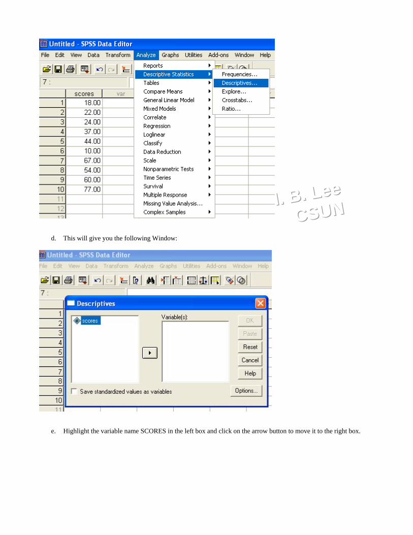
3. Analyze the data.a. Choose Analyze from the Top Row of Action in the SPSS screen.b. With the drop down menu choose DESCRIPTIVE STATISTICSc. This will give you another menu. From this menu choose DESCRIPTIVES.


d. This will give you the following Window:

e. Highlight the variable name SCORES in the left box and click on the arrow button to move it to the right box.


f. Click on OK and the analysis will run.g. The output is given below:

Descriptives

Descriptive Statistics

10 10.00 77.00 41.3000 22.7696210

scoresValid N (listwise)

N Minimum Maximum Mean Std. Deviation

SPSS Instructions for Correlation

Given the following age and error scores on an ability test for a small sample of boys, find the correlation: (8,8);(6,12); (12,5); (15,1); (10,10); (5,15); (12,5); (9,10); (13,3); (10,9).

Find the Pearson correlation between age and error scores using SPSS.

1. Define the variables.a. Go to Variable View (Use Tab on lower left corner of the SPSS screen).b. For correlation we have two sets of scores, we need to name both. Name the first variable AGE and the secondvariable as SCORES


.c. Return to Data View (using tab on lower left corner of SPSS screen).

2. Under the column “AGE” and “SCORES”, enter the data given above.

The Data Table should look like:

3. Analyze the data.a. Choose Analyze from the Top Row of Actions in the SPSS screen.b. With the drop down menu choose CORRELATEc. This will give you another menu. From this menu choose BIVARIATE.


d. Click on “BIVARIATE” and you will get the following window:

e. Move both variables from the left box to the right box, by highlighting the variables and clicking on the arrowbutton.

f. Click on the OPTIONS button and place a check mark in the box “Means and standard deviations.” Click onCONTINUE button.

g. Click on OK button to do analysis.

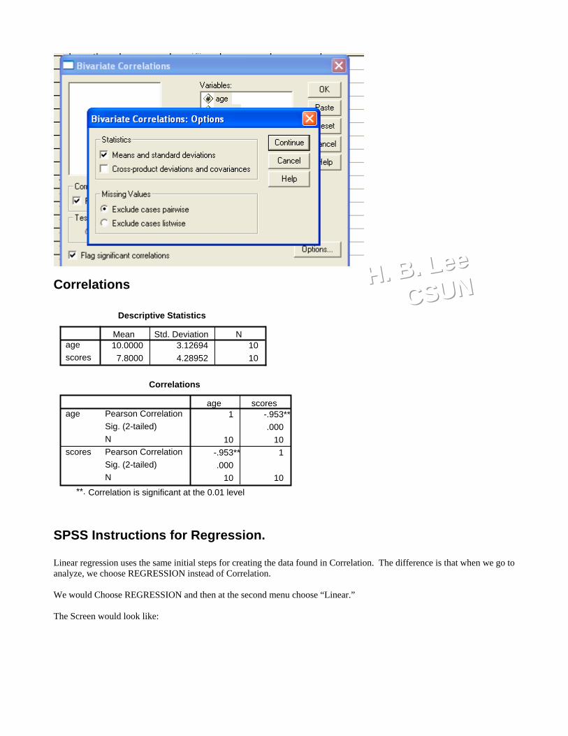
HHH... BBB... LLLeeeeee CCCSSSUUUNNN Correlations


10.0000 3.12694 107.8000 4.28952 10

agescores

Mean Std. Deviation N

Correlations

1 -.953**.000

10 10-.953** 1.000

10 10

Pearson CorrelationSig. (2-tailed)NPearson CorrelationSig. (2-tailed)N

age

scores

age scores

Correlation is significant at the 0.01 level(2 il d)

**.

SPSS Instructions for Regression.

Linear regression uses the same initial steps for creating the data found in Correlation. The difference is that when we go toanalyze, we choose REGRESSION instead of Correlation.

We would Choose REGRESSION and then at the second menu choose “Linear.”

The Screen would look like:


When we make our choice, we get the following window:

If we were to predict scores based on age, we would move the variable AGE from the left box into the box labeled“Independent(s).” Likewise, we would move the variable “SCORES” from the left box into the box labeled“Dependent.” The window below shows this.


To obtain descriptive statistics with regression Click on the “STATISTICS” box at the bottom of the screen. This willgive a window box where you would place a check mark in the box labeled “Descriptives.” Click on the CONTINUEbutton.

If we now click on the “OK” button the analysis will begin and give an output.

Regression



7.8000 4.28952 1010.0000 3.12694 10

scoresage


Correlations

1.000 -.953-.953 1.000

. .000.000 .

10 1010 10

scoresagescoresagescoresage

Pearson Correlation

Sig. (1-tailed)

N

scores age

Variables Entered/Removedb

agea . EnterModel1

VariablesEntered

VariablesRemoved Method

All requested variables entered.a.

Dependent Variable: scoresb.

Model Summary

.953a .908 .896 1.38365Model1

R R SquareAdjustedR Square

Std. Error ofthe Estimate

Predictors: (Constant), agea.

ANOVAb

150.284 1 150.284 78.498 .000a

15.316 8 1.914165.600 9

RegressionResidualTotal

Model1

Sum ofSquares df Mean Square F Sig.

Predictors: (Constant), agea.

Dependent Variable: scoresb.

Coefficientsa

20.868 1.539 13.564 .000-1.307 .147 -.953 -8.860 .000

(Constant)age

Model1

B Std. Error

UnstandardizedCoefficients

Beta

StandardizedCoefficients

t Sig.

Dependent Variable: scoresa.

The regression weights are found in the last output section. It is the Unstandardized Coefficients B.


SPSS Instructions for Correlated Samples t-test.The data for this example is

A human factors psychologist developed a research study to see if a certain keyboard reduces the number ofhand and finger injuries. The researcher recruited 7 staff members from the word processing pool. Each personwas randomly assigned to receive the original keyboard or the new keyboard. This was done in an attempt toeliminate order effects. Each person was asked to type 25 pages of text with an apparatus strapped to each handto determine the amount of stress placed on each finger and hand ligament. The data are given below, wherehigher values indicate higher stress and greater likelihood of finger and hand injuries. Conduct the appropriatehypothesis test to determine if the new keyboard is better than the old keyboard. Note: if the new keyboard isbetter, we would expect it to place less stress on the hands. Use α = .01.

Old 25 33 36 29 44 19 39New 16 27 33 30 28 19 22

The correlated samples (groups) t-test uses the same initial steps for creating the data found in Correlation and regression.There are two variables defined

The difference is that when we go to analyze, we choose COMPARE MEANS instead of Correlation or Regression.

We would Choose COMPARE MEANS and then at the second menu choose “Paired Sample T-Test.”

The Screen would look like:


After making our choice we get the following window:

The next step is to highlight the two variables in the left box and then click on the Arrow button. When we do so, weget the following window screen:


By now clicking on the OK button, the analysis will run and give the following output:

T-Test

Paired Samples Statistics

32.1429 7 8.53285 3.2251125.0000 7 6.16441 2.32993

oldnew

Pair1

Mean N Std. DeviationStd. Error

Mean

Paired Samples Correlations

7 .554 .196old & newPair 1N Correlation Sig.

Paired Samples Test

7.14286 7.24405 2.73799 .44323 13.842 2.609 6 .040old - newPair 1Mean

Std.Deviation

Std.ErrorMean Lower Upper

95% ConfidenceInterval of the

Difference

Paired Differences

t dfSig.

(2-tailed)

SPSS Instructions for a One Sample t-test.

A written claim included with each stereo made by a certain electronics appliance manufacturer states that eachstereo unit is guaranteed to last 5 years without any defects. Six individuals purchased units, and all six units failbefore 5 years. The failure times in years are 3.9, 4.6, 3.8, 4.7, 4.8, and 4.1, respectively. Develop theappropriate hypothesis test to determine whether or not there is evidence to contradict the manufacturer's claim.Use α = .05.

The setup for this test is very similar to the setup we initially used to find the mean and standard deviation of a singleset of values.

1. We go to Define Variables and define one variable called “YEARS”2. WE then return to Data View and enter the values given in the problem presented above. The SPSS data table would

look like:


3. Next, from Analyze, we choose “COMPARE MEANS” and then choose :One Sample T-Test.” The screen will looklike:

4. After clicking on “One Sample T-Test,” we get the following screen:

5. Highlight the variable “YEARS” in the left box and move it to the right box. In the box labeled “Test Value” put thevalue found in the null hypothesis. In this case, the value is “5.”


6. Click on the “OK” button to do the analysis and get the output.

T-Test

One-Sample Statistics

6 4.3167 .43551 .17780yearsN Mean Std. Deviation

Std. ErrorMean

One-Sample Test

-3.843 5 .012 -.68333 -1.1404 -.2263yearst df Sig. (2-tailed)

MeanDifference Lower Upper


Difference

Test Value = 5

SPSS Instructions for Uncorrelated Samples t-test.

An industrial psychologist conducted a study to see if there is any difference between hourly-paid workers andsalary workers in terms of attendance. As a measure of attendance, the researcher used the number of absencesover a 3-month period. The data from 10 salary and 10 hourly workers are given below. Conduct theappropriate hypothesis test to determine if there are any differences between hourly and salary workers in termsof amount of sick leave taken.

Hourly 2 2 1 3 4 2 1 4 1 2Salary 2 5 2 7 2 4 1 3 4 2

The two uncorrrelated samples t-test is set up differently than the two correlated samples t-test. There are still two variablesto be defined, but their definitions are different. With a two uncorrelated samples t-test, one of the variables to be defined isthe outcome variable. In the example given above, it would be the number of absences. We would define a variable“ABSENT.” The second variable defined group membership. There are two groups: Salary and Hourly. Each membership


serves as one level of the variable to be defined (explanatory or independent variable). The variable would be “WORKER.”Or worker type.

1. So in Variable View, we define one variable as ABSENT and the other as WORKER.2. We return to Data View and enter in the data. For ABSENT, we would put in the values as shown in the example

given above. However, for the second variable WORKER, we would use the number “1” to define Hourly and thenumber “2” for Salary. The DATA Table would look like:

3. From ANALYZE, choose “COMPARE MEANS” and then “Independent Sample T-Test.”

4. When this is chosen, the following window appears:


5. Move ABSENT from the left box into the box labeled “Test Variable(s).”6. Move WORKER from the left box into the box labeled “Grouping Variable.”

7. You will notice that WORKER is now in the box labeled “Grouping Variable.” However, parentheses and 2 questionmarks follow it. SPSS is asking us to define the two groups to be used. We had designated “!” for Hourly and a “2” forSalary. We need to tell SPSS this. We do this by clicking on the button just below it “Define Groups.” When we dothis we get the following window:

8. We now type in the number “1” in the Group 1 box and “2” in the Group 2 box, and then clock on the “CONTINUE”button.


9. The Question marks for WORKER have now been replaced with the values we entered:

10. We can do the analysis now by clicking on the OK button.

T-Test

Group Statistics

10 2.2000 1.13529 .3590110 3.2000 1.81353 .57349

worker1.002.00

absentN Mean Std. Deviation

Std. ErrorMean

Independent Samples Test

2.219 .154 -1.478 18 .157 .67659 -2.4215 .42147

-1.478 15.11 .160 .67659 -2.4412 .44117

Equal variancesassumedEqual variancesnot assumed

absentF Sig.

Levene's Test forEquality ofVariances

t dfSig.

(2-tailed)

Std.ErrorDiffer Lower Upper


Difference

t-test for Equality of Means


SPSS Instructions for One Way ANOVA

A consumer research company is hired to see if three additives used in automobile gasoline improves mileage. Twelve carsof the same make, year, and model are used in the study. The data after three tanks of gasoline are given below.

Additive Average miles pergallon

SVT

232021

251924

262118

221719

The one-way ANOVA is an extension of the uncorrelated samples t-test. There are two variables: An outcome ordependent variable and a grouping or independent variable.

For the example given above, the outcome variable is miles per gallon (MPG) and the grouping variable is ADDITIVES.For ADDITIVES, there are 3 kinds or levels. Hence we will numerically designate additive S as “1”, additive V as “2” andadditive T as “3.”

1. In SPSS we define the two variables through Variable View. We will define and use MPG and ADDITIVE. We thenreturn to Data View and enter in the values. The data table for this problem would look like:

2. From ANALYZE choose “COMPARE MEANS” and then “ONE-WAY ANOVA.” The window you get when this isdone is


3. Move MPG from the left box to the box labeled “Dependent List.” Move ADDITIVE from the left box to the boxlabeled "Factor."

When this is done you get the following window:

4. Click on the “POST HOC” button and place a check mark in the boxes for SCHEFFE and TUKEY. After doing so,click on the “CONTINUE” button.


5. Next click on the “OPTIONS” button and place a check mark in the box for Descriptive Statistics.. Click on theCONTINUE button.

6. You will then return to the previous Window. From this window click on the OK button to run the analysis.

Oneway


Descriptives

mpg

4 24.0000 1.82574 .91287 21.0948 26.9052 22.00 26.004 19.2500 1.70783 .85391 16.5325 21.9675 17.00 21.004 20.5000 2.64575 1.32288 16.2900 24.7100 18.00 24.00

12 21.2500 2.83244 .81766 19.4504 23.0496 17.00 26.00

1.002.003.00Total

N MeanStd.

DeviationStd.Error

LowerBound

UpperBound

95% ConfidenceInterval for Mean

Min Max

ANOVA

mpg

48.500 2 24.250 5.491 .02839.750 9 4.41788.250 11

Between GroupsWithin GroupsTotal

Sum ofSquares df Mean Square F Sig.

Post Hoc Tests

Multiple Comparisons

Dependent Variable: mpg

4.75000* 1.48605 .027 .6010 8.89903.50000 1.48605 .098 -.6490 7.6490

-4.75000* 1.48605 .027 -8.8990 -.6010-1.25000 1.48605 .688 -5.3990 2.8990-3.50000 1.48605 .098 -7.6490 .64901.25000 1.48605 .688 -2.8990 5.39904.75000* 1.48605 .033 .4142 9.08583.50000 1.48605 .115 -.8358 7.8358

-4.75000* 1.48605 .033 -9.0858 -.4142-1.25000 1.48605 .711 -5.5858 3.0858-3.50000 1.48605 .115 -7.8358 .83581.25000 1.48605 .711 -3.0858 5.5858

(J) additive2.003.001.003.001.002.002.003.001.003.001.002.00

(I) additive1.00

2.00

3.00

1.00

2.00

3.00

Tukey HSD

Scheffe

MeanDifference

(I-J)Std.Error Sig.

LowerBound

UpperBound

95% ConfidenceInterval

The mean difference is significant at the .05 level.*.

Homogeneous Subsets


mpg

4 19.25004 20.5000 20.50004 24.0000

.688 .0984 19.25004 20.5000 20.50004 24.0000

.711 .115

additive2.003.001.00Sig.2.003.001.00Sig.

Tukey HSDa

Scheffea

N 1 2Subset for alpha = .05

Means for groups in homogeneous subsets are displayed.Uses Harmonic Mean Sample Size = 4.000.a.

SPSS Instructions for TWO-Way ANOVAA professor of physical education is conducting a study on whether the amount physical exercise and time pf day when theexercise is done affects nighttime sleep. There are 3 levels of exercise: light, moderate and heavy and two levels for time ofday: morning and evening. Eighteen college students in good health were randomly recruited and assigned to the 6treatment conditions. Each participant exercised only once and the amount of sleep obtained for that night was recorded.The data are given below:

Light Moderate HeavyMorning 6.5 7.3 7.2 7.3 7.6 6.8 7.6 6.6 7.2Evening 7.1 7.9 8.2 7.4 8.1 8.2 8.2 8.5 9.3 To do this problem in SPSS, we need to define 3 variables. There are two independent variables: AMOUNT and TIME.There is one dependent variable: HOURS of sleep.

1. In Variable View, define three variables: HOURS, AMOUNT and TIME. Then return to Data View and enter in thedata values. For AMOUNT use “1” for light, “2” for moderate and “ 3” for heavy. For TIME, use “1” for morningand “2” for evening. The SPSS data table would look like:


2. From ANALYZE, choose “General Linear Model” and then “Univariate.”

3. When we do this we get the follow window:


4. Move AMOUNT and TIME from the left box to the box labeled “Fixed Factor(s),” and move HOURS to the boxlabeled “Dependent Variable.” When this is done, the window will look like:

5. Click on the POST HOC button. When this is done, you will get a window where you will move the AMOUNTvariable from the left box (Factors) to the right-side box (Post Hoc Tests for). You will then place a check mark nextto the boxes SCHEFFE and TUKEY. Click on the CONTINUE button.


6. When you return to the original Univariate Window, clcik on the OK button to do the analysis.

Univariate Analysis of Variance

Between-Subjects Factors

66699

1.002.003.00

amount

1.002.00

time

N

Tests of Between-Subjects Effects

Dependent Variable: hours

5.871a 5 1.174 4.881 .0111042.722 1 1042.722 4334.642 .000

.871 2 .436 1.811 .2054.302 1 4.302 17.885 .001

.698 2 .349 1.450 .2732.887 12 .241

1051.480 188.758 17

SourceCorrected ModelInterceptamounttimeamount * timeErrorTotalCorrected Total

Type III Sumof Squares df

MeanSquare F Sig.

R Squared = .670 (Adjusted R Squared = .533)a.

Post Hoc Tests


amount

Multiple Comparisons

Dependent Variable: hours

-.2000 .28317 .764 -.9555 .5555-.5333 .28317 .186 -1.2888 .2221.2000 .28317 .764 -.5555 .9555

-.3333 .28317 .488 -1.0888 .4221.5333 .28317 .186 -.2221 1.2888.3333 .28317 .488 -.4221 1.0888

-.2000 .28317 .783 -.9894 .5894-.5333 .28317 .211 -1.3227 .2560.2000 .28317 .783 -.5894 .9894

-.3333 .28317 .519 -1.1227 .4560.5333 .28317 .211 -.2560 1.3227.3333 .28317 .519 -.4560 1.1227

(J) amount2.003.001.003.001.002.002.003.001.003.001.002.00

(I) amount1.00

2.00

3.00

1.00

2.00

3.00

Tukey HSD

Scheffe

MeanDifference

(I-J)Std.Error Sig.

LowerBound

UpperBound

95% ConfidenceInterval

Based on observed means.

Homogeneous Subsets

hours

6 7.36676 7.56676 7.9000

.1866 7.36676 7.56676 7.9000

.211

amount1.002.003.00Sig.1.002.003.00Sig.

Tukey HSDa,b

Scheffea,b

N 1Subset

Means for groups in homogeneous subsets are displayed.Based on Type III Sum of SquaresThe error term is Mean Square(Error) = .241.

Uses Harmonic Mean Sample Size = 6.000.a.

Alpha = .05.b.


SPSS Instructions for a One-Way Repeated Measures ANOVA The one-way repeated measures ANOVA is an extension of the correlated samples t-test. With the correlated t-test, there were two groups that are correlated in that the same participant was measured twice on the same or similar variable. The participant was essentially matched or paired with oneself. With the one-way repeated measures ANOVA, each participant is measured more than twice on the same or similar dependent variable or outcome measure. For example, 9 participants were measured over a 5-week period on the number of migraine headaches. The first two weeks were used develop a baseline measure followed by 3 weeks of self-therapy. The design of a study involving measurement of each participant on the same dependent variable over 5 occasions is given as:

Participants Week 1 Week 2 Week 3 Week 4 Week 5 1 2 3 4 5 6 7 8 9

21 20 17 25 30 19 26 17 26

22 19 15 30 27 27 16 18 24

8 10 5

13 13 8 5 8

14

6 4 4

12 8 7 2 1 8

6 4 5

17 6 4 5 5 9

This information is entered into SPSS and the data table will look like:

Next, select “Analyze” and on the submenu point the mouse cursor to “General Linear Model.” Doing this will give yet another submenu. Select from this submenu “Repeated Measures.”


This will open up a window. In the window, replace “factor1” with “WEEK” in the Within Subjects Factor Name. In the number of levels box, enter in the number “5.”

After doing this, click on the “Add” button. Following this action click on the “Define” button. This in turn will open another window: Within this window, highlight “week1,” “week2,”… , “Week5” and move them from the left box to the top rightmost box. This will replace the _?_[1], _?_[2], . . , _?_[5] with the week names and show week1[1], week2[2], . . . , week5[5].


If one wants to, they can click on the “Post Hoc” button to request post hoc tests. For descriptive statistics, click on the “Options” button. This will give a window where the user can select “Descriptive Statistics” and any of the listed statistics. Move “OVERALL” from the left box to the right box. When finished with selections, click on the “Continue” button. This will return the user back to the previous window. Click on the “OK” button to run the analysis.


SPSS generates more output than needed by the researcher. Given below are those pieces of output that are the most useful to the researcher.


22.33 4.583 922.00 5.339 9

9.33 3.391 95.78 3.420 96.78 4.116 9

week1week2week3week4week5


Tests of Within-Subjects Effects

Measure: MEASURE_1

2449.200 4 612.300 85.042 .0002449.200 2.738 894.577 85.042 .0002449.200 4.000 612.300 85.042 .0002449.200 1.000 2449.2 85.042 .000230.400 32 7.200230.400 21.903 10.519230.400 32.000 7.200230.400 8.000 28.800

Sphericity AssumedGreenhouse-GeisserHuynh-FeldtLower-boundSphericity AssumedGreenhouse-GeisserHuynh-FeldtLower-bound

SourceWEEK

Error(WEEK)

Type III Sumof Squares df

MeanSquare F Sig.

The line “Sphericity Assumed” is the one used if the research does not suspect any problems with the data. The other 3 tests are considered to be conservative tests. SPSS Instructions for a Two-Way Mixed ANOVA


In a mixed 2-way ANOVA, one of the IVs creates uncorrelated groups and the second creates correlated groups. For example, if a researcher wanted to study sex differences on a verbal task, this variable “sex” would create uncorrelated groups. If the researcher measured the participants before and after some kind of intervention (new teaching method) in on a verbal test, the testing sessions would result in correlated groups. Hence the design would look like:

Sex Before Treatment After Treatment Women S1 S2 S3 S4 S5 S1 S2 S3 S4 S5 Men S6 S7 S8 S9 S10 S6 S7 S8 S9 S10

Note that there are five different women (S1 S2 S3 S4 S5) and five different men (S6 S7 S8 S9 S10) measured before treatment and then again after treatment. Women and men or Sex constitutes the uncorrelated grouping while before treatment and after treatment or just Time makes up the correlated grouping. Using actual data values, the table looks like:

Sex Before Treatment After Treatment Women 15, 10, 8, 11, 9 16, 14, 6, 12, 10 Men 4, 8, 16, 12, 10 6, 9, 15, 13, 11

In SPSS, three variables are created: SEX, BEFORE and AFTER. The appropriate data values are added into the SPSS Data Table. This is what it would look like:

Click on “ANALYZE” at the top menu bar. From ANALYZE, choose “General Lineal Model.” From the submenu choose “Repeated Measures.”


When clicking on “Repeated Measures, a window will appear:

Replace “factor1” in the Within Subject Factor Name box with a more appropriate one for the analysis. For this

particular study it would be “TIME.” In the Number of Levels box put in the number “2”. This says there are two time periods (Before – After). If a research had 3 time periods or trials, then the number “3” would be entered in the box.

After putting the number “2” in the box, click on the button “ADD.” Follow this with a click on the button “Define.” When this is done another window will appear on the screen. On the left box the name of the three variables will appear. The task now is to move the appropriate variables into the correct boxes on the right side.


Select “before” and “after” and move them into the first box. The _?_[1} and _?_[2} will be replaced by before[1] and after[2]. Select and move “sex” from the left box into the box labeled Between Subjects Factor(s).


If post hoc tests are needed, they can be obtained from clicking the “post hoc” button. To obtain descriptive statistics, click on the “Options” button. It will bring a screen that looks like:

Select “Descriptive Statistics” and any other pertinent measure such as “Estimates of Effect Size.” Move “OVERALL” from the left box to the right box. Then click on “Continue.” This will return you back to the previous window. To do the analyses, click on the “OK” button. The needed information will be found in different places in the output. SPSS generates a lot of output. Only the pertinent ones were extracted and presented in this document. The first gives the non-conservative and conservative tests for the within subjects factor (correlated groups), TIME and the interaction between TIME and SEX. The second hives the analysis for the between subjects factor (uncorrelated groups): SEX.

Tests of Within-Subjects Effects

Measure: MEASURE_1

4.050 1 4.050 2.104 .1854.050 1.000 4.050 2.104 .1854.050 1.000 4.050 2.104 .1854.050 1.000 4.050 2.104 .185

.050 1 .050 .026 .876

.050 1.000 .050 .026 .876

.050 1.000 .050 .026 .876

.050 1.000 .050 .026 .87615.400 8 1.92515.400 8.000 1.92515.400 8.000 1.92515.400 8.000 1.925

Sphericity AssumedGreenhouse-GeisserHuynh-FeldtLower-boundSphericity AssumedGreenhouse-GeisserHuynh-FeldtLower-boundSphericity AssumedGreenhouse-GeisserHuynh-FeldtLower-bound

SourceTIME

TIME * sex

Error(TIME)

Type III Sumof Squares df Mean Square F Sig.


Tests of Between-Subjects Effects

Measure: MEASURE_1Transformed Variable: Average

2311.250 1 2311.250 91.625 .0002.450 1 2.450 .097 .763

201.800 8 25.225

SourceInterceptsexError

Type III Sumof Squares df Mean Square F Sig.

Documents

SPSS Instructions for Descriptive Statistics