SPSS Advanced Models™ 15 - Brock University · To install the SPSS Advanced Models add-on module, ... Your serial number is your identiﬁcation number with SPSS Inc. You will need

SPSS Advanced Models™ 15.0

For more information about SPSS® software products, please visit our Web site at http://www.spss.com or contact

SPSS Inc.233 South Wacker Drive, 11th FloorChicago, IL 60606-6412Tel: (312) 651-3000Fax: (312) 651-3668

SPSS is a registered trademark and the other product names are the trademarks of SPSS Inc. for its proprietary computer software. No materialdescribing such software may be produced or distributed without the written permission of the owners of the trademark and license rights in thesoftware and the copyrights in the published materials.

The SOFTWARE and documentation are provided with RESTRICTED RIGHTS. Use, duplication, or disclosure by the Government issubject to restrictions as set forth in subdivision (c) (1) (ii) of The Rights in Technical Data and Computer Software clause at 52.227-7013.Contractor/manufacturer is SPSS Inc., 233 South Wacker Drive, 11th Floor, Chicago, IL 60606-6412.Patent No. 7,023,453

General notice: Other product names mentioned herein are used for identification purposes only and may be trademarks of their respectivecompanies.

TableLook is a trademark of SPSS Inc.Windows is a registered trademark of Microsoft Corporation.DataDirect, DataDirect Connect, INTERSOLV, and SequeLink are registered trademarks of DataDirect Technologies.Portions of this product were created using LEADTOOLS © 1991–2000, LEAD Technologies, Inc. ALL RIGHTS RESERVED.LEAD, LEADTOOLS, and LEADVIEW are registered trademarks of LEAD Technologies, Inc.Sax Basic is a trademark of Sax Software Corporation. Copyright © 1993–2004 by Polar Engineering and Consulting. All rights reserved.A portion of the SPSS software contains zlib technology. Copyright © 1995–2002 by Jean-loup Gailly and Mark Adler. The zlib software isprovided “as is,” without express or implied warranty.A portion of the SPSS software contains Sun Java Runtime libraries. Copyright © 2003 by Sun Microsystems, Inc. All rights reserved. TheSun Java Runtime libraries include code licensed from RSA Security, Inc. Some portions of the libraries are licensed from IBM and areavailable at http://www-128.ibm.com/developerworks/opensource/.

SPSS Advanced Models™ 15.0Copyright © 2006 by SPSS Inc.All rights reserved.Printed in the United States of America.

No part of this publication may be reproduced, stored in a retrieval system, or transmitted, in any form or by any means, electronic, mechanical,photocopying, recording, or otherwise, without the prior written permission of the publisher.

1 2 3 4 5 6 7 8 9 0 09 08 07 06

ISBN-13: 978-1-56827-384-6ISBN-10: 1-56827-384-3

Preface

SPSS 15.0 is a comprehensive system for analyzing data. The SPSS Advanced Modelsoptional add-on module provides the additional analytic techniques described in this manual.The Advanced Models add-on module must be used with the SPSS 15.0 Base system and iscompletely integrated into that system.

Installation

To install the SPSS Advanced Models add-on module, run the License Authorization Wizardusing the authorization code that you received from SPSS Inc. For more information, see theinstallation instructions supplied with the SPSS Advanced Models add-on module.

Compatibility

SPSS is designed to run on many computer systems. See the installation instructions that camewith your system for specific information on minimum and recommended requirements.

Serial Numbers

Your serial number is your identification number with SPSS Inc. You will need this serial numberwhen you contact SPSS Inc. for information regarding support, payment, or an upgraded system.The serial number was provided with your Base system.

Customer Service

If you have any questions concerning your shipment or account, contact your local office, listedon the SPSS Web site at http://www.spss.com/worldwide. Please have your serial number readyfor identification.

Training Seminars

SPSS Inc. provides both public and onsite training seminars. All seminars featurehands-on workshops. Seminars will be offered in major cities on a regular basis. For moreinformation on these seminars, contact your local office, listed on the SPSS Web site athttp://www.spss.com/worldwide.

Technical Support

The services of SPSS Technical Support are available to maintenance customers. Customersmay contact Technical Support for assistance in using SPSS or for installation help for oneof the supported hardware environments. To reach Technical Support, see the SPSS Web

iii

site at http://www.spss.com, or contact your local office, listed on the SPSS Web site athttp://www.spss.com/worldwide. Be prepared to identify yourself, your organization, and theserial number of your system.

Additional Publications

Additional copies of SPSS product manuals may be purchased directly from SPSS Inc. Visit theSPSS Web Store at http://www.spss.com/estore, or contact your local SPSS office, listed on theSPSS Web site at http://www.spss.com/worldwide. For telephone orders in the United States andCanada, call SPSS Inc. at 800-543-2185. For telephone orders outside of North America, contactyour local office, listed on the SPSS Web site.The SPSS Statistical Procedures Companion, by Marija Norušis, has been published by

Prentice Hall. A new version of this book, updated for SPSS 15.0, is planned. The SPSSAdvanced Statistical Procedures Companion, also based on SPSS 15.0, is forthcoming. TheSPSS Guide to Data Analysis for SPSS 15.0 is also in development. Announcements ofpublications available exclusively through Prentice Hall will be available on the SPSS Web site athttp://www.spss.com/estore (select your home country, and then click Books).

Tell Us Your Thoughts

Your comments are important. Please let us know about your experiences with SPSS products.We especially like to hear about new and interesting applications using the SPSS AdvancedModels add-on module. Please send e-mail to [email protected] or write to SPSS Inc., Attn.:Director of Product Planning, 233 South Wacker Drive, 11th Floor, Chicago, IL 60606-6412.

About This Manual

This manual documents the graphical user interface for the procedures included in the SPSSAdvanced Models add-on module. Illustrations of dialog boxes are taken from SPSS forWindows. Dialog boxes in other operating systems are similar. Detailed information about thecommand syntax for features in the SPSS Advanced Models add-on module is available in twoforms: integrated into the overall Help system and as a separate document in PDF form in theSPSS 15.0 Command Syntax Reference, available from the Help menu.

Contacting SPSS

If you would like to be on our mailing list, contact one of our offices, listed on our Web siteat http://www.spss.com/worldwide.

iv

Contents

1 Introduction to SPSS Advanced Models 1

2 GLM Multivariate Analysis 2

GLM Multivariate Model . . . . . . . . . . . . . . . . . . . . . . . . . . . . . . . . . . . . . . . . . . . . . . . . . . . . . . . . 4Build Terms . . . . . . . . . . . . . . . . . . . . . . . . . . . . . . . . . . . . . . . . . . . . . . . . . . . . . . . . . . . . . . 5Sum of Squares . . . . . . . . . . . . . . . . . . . . . . . . . . . . . . . . . . . . . . . . . . . . . . . . . . . . . . . . . . . 5

GLM Multivariate Contrasts . . . . . . . . . . . . . . . . . . . . . . . . . . . . . . . . . . . . . . . . . . . . . . . . . . . . . 6Contrast Types. . . . . . . . . . . . . . . . . . . . . . . . . . . . . . . . . . . . . . . . . . . . . . . . . . . . . . . . . . . . 7

GLM Multivariate Profile Plots . . . . . . . . . . . . . . . . . . . . . . . . . . . . . . . . . . . . . . . . . . . . . . . . . . . 7GLM Multivariate Post Hoc Comparisons . . . . . . . . . . . . . . . . . . . . . . . . . . . . . . . . . . . . . . . . . . . 8GLM Save. . . . . . . . . . . . . . . . . . . . . . . . . . . . . . . . . . . . . . . . . . . . . . . . . . . . . . . . . . . . . . . . . . 10GLM Multivariate Options . . . . . . . . . . . . . . . . . . . . . . . . . . . . . . . . . . . . . . . . . . . . . . . . . . . . . . 11GLM Command Additional Features . . . . . . . . . . . . . . . . . . . . . . . . . . . . . . . . . . . . . . . . . . . . . . 12

3 GLM Repeated Measures 14

GLM Repeated Measures Define Factors . . . . . . . . . . . . . . . . . . . . . . . . . . . . . . . . . . . . . . . . . . 17GLM Repeated Measures Model . . . . . . . . . . . . . . . . . . . . . . . . . . . . . . . . . . . . . . . . . . . . . . . . 18

Build Terms . . . . . . . . . . . . . . . . . . . . . . . . . . . . . . . . . . . . . . . . . . . . . . . . . . . . . . . . . . . . . 18Sum of Squares . . . . . . . . . . . . . . . . . . . . . . . . . . . . . . . . . . . . . . . . . . . . . . . . . . . . . . . . . . 19

GLM Repeated Measures Contrasts . . . . . . . . . . . . . . . . . . . . . . . . . . . . . . . . . . . . . . . . . . . . . . 20Contrast Types. . . . . . . . . . . . . . . . . . . . . . . . . . . . . . . . . . . . . . . . . . . . . . . . . . . . . . . . . . . 20

GLM Repeated Measures Profile Plots . . . . . . . . . . . . . . . . . . . . . . . . . . . . . . . . . . . . . . . . . . . . 21GLM Repeated Measures Post Hoc Comparisons . . . . . . . . . . . . . . . . . . . . . . . . . . . . . . . . . . . . 22GLM Repeated Measures Save. . . . . . . . . . . . . . . . . . . . . . . . . . . . . . . . . . . . . . . . . . . . . . . . . . 24GLM Repeated Measures Options . . . . . . . . . . . . . . . . . . . . . . . . . . . . . . . . . . . . . . . . . . . . . . . 25GLM Command Additional Features . . . . . . . . . . . . . . . . . . . . . . . . . . . . . . . . . . . . . . . . . . . . . . 26

v

4 Variance Components Analysis 28

Variance Components Model . . . . . . . . . . . . . . . . . . . . . . . . . . . . . . . . . . . . . . . . . . . . . . . . . . . 30Build Terms . . . . . . . . . . . . . . . . . . . . . . . . . . . . . . . . . . . . . . . . . . . . . . . . . . . . . . . . . . . . . 30

Variance Components Options . . . . . . . . . . . . . . . . . . . . . . . . . . . . . . . . . . . . . . . . . . . . . . . . . . 31Sum of Squares (Variance Components) . . . . . . . . . . . . . . . . . . . . . . . . . . . . . . . . . . . . . . . 32

Variance Components Save to New File . . . . . . . . . . . . . . . . . . . . . . . . . . . . . . . . . . . . . . . . . . . 33VARCOMP Command Additional Features . . . . . . . . . . . . . . . . . . . . . . . . . . . . . . . . . . . . . . . . . . 33

5 Linear Mixed Models 34

Linear Mixed Models Select Subjects/Repeated Variables . . . . . . . . . . . . . . . . . . . . . . . . . . . . . 36Linear Mixed Models Fixed Effects . . . . . . . . . . . . . . . . . . . . . . . . . . . . . . . . . . . . . . . . . . . . . . . 38

Build Non-Nested Terms . . . . . . . . . . . . . . . . . . . . . . . . . . . . . . . . . . . . . . . . . . . . . . . . . . . 38Build Nested Terms . . . . . . . . . . . . . . . . . . . . . . . . . . . . . . . . . . . . . . . . . . . . . . . . . . . . . . . 39Sum of Squares . . . . . . . . . . . . . . . . . . . . . . . . . . . . . . . . . . . . . . . . . . . . . . . . . . . . . . . . . . 39

Linear Mixed Models Random Effects . . . . . . . . . . . . . . . . . . . . . . . . . . . . . . . . . . . . . . . . . . . . . 40Linear Mixed Models Estimation . . . . . . . . . . . . . . . . . . . . . . . . . . . . . . . . . . . . . . . . . . . . . . . . . 42Linear Mixed Models Statistics. . . . . . . . . . . . . . . . . . . . . . . . . . . . . . . . . . . . . . . . . . . . . . . . . . 43Linear Mixed Models EM Means . . . . . . . . . . . . . . . . . . . . . . . . . . . . . . . . . . . . . . . . . . . . . . . . 44Linear Mixed Models Save . . . . . . . . . . . . . . . . . . . . . . . . . . . . . . . . . . . . . . . . . . . . . . . . . . . . . 45MIXED Command Additional Features. . . . . . . . . . . . . . . . . . . . . . . . . . . . . . . . . . . . . . . . . . . . . 45

6 Generalized Linear Models 47

Generalized Linear Models Reference Category . . . . . . . . . . . . . . . . . . . . . . . . . . . . . . . . . . . . . 50Generalized Linear Models Predictors . . . . . . . . . . . . . . . . . . . . . . . . . . . . . . . . . . . . . . . . . . . . 51

Generalized Linear Models Options . . . . . . . . . . . . . . . . . . . . . . . . . . . . . . . . . . . . . . . . . . . 52Generalized Linear Models Model . . . . . . . . . . . . . . . . . . . . . . . . . . . . . . . . . . . . . . . . . . . . . . . 53Generalized Linear Models Estimation . . . . . . . . . . . . . . . . . . . . . . . . . . . . . . . . . . . . . . . . . . . . 54

Generalized Linear Models Initial Values . . . . . . . . . . . . . . . . . . . . . . . . . . . . . . . . . . . . . . . 56Generalized Linear Models Statistics . . . . . . . . . . . . . . . . . . . . . . . . . . . . . . . . . . . . . . . . . . . . . 57Generalized Linear Models EM Means . . . . . . . . . . . . . . . . . . . . . . . . . . . . . . . . . . . . . . . . . . . . 59Generalized Linear Models Save. . . . . . . . . . . . . . . . . . . . . . . . . . . . . . . . . . . . . . . . . . . . . . . . . 61Generalized Linear Models Export . . . . . . . . . . . . . . . . . . . . . . . . . . . . . . . . . . . . . . . . . . . . . . . 62GENLIN Command Additional Features . . . . . . . . . . . . . . . . . . . . . . . . . . . . . . . . . . . . . . . . . . . . 63

vi

7 Generalized Estimating Equations 64

Generalized Estimating Equations Response . . . . . . . . . . . . . . . . . . . . . . . . . . . . . . . . . . . . . . . . 67Generalized Estimating Equations Reference Category . . . . . . . . . . . . . . . . . . . . . . . . . . . . 69

Generalized Estimating Equations Predictors . . . . . . . . . . . . . . . . . . . . . . . . . . . . . . . . . . . . . . . 70Generalized Estimating Equations Options . . . . . . . . . . . . . . . . . . . . . . . . . . . . . . . . . . . . . . 71

Generalized Estimating Equations Model . . . . . . . . . . . . . . . . . . . . . . . . . . . . . . . . . . . . . . . . . . 72Generalized Estimating Equations Estimation . . . . . . . . . . . . . . . . . . . . . . . . . . . . . . . . . . . . . . . 73

Generalized Estimating Equations Initial Values . . . . . . . . . . . . . . . . . . . . . . . . . . . . . . . . . . 75Generalized Estimating Equations Statistics . . . . . . . . . . . . . . . . . . . . . . . . . . . . . . . . . . . . . . . . 76Generalized Estimating Equations EM Means . . . . . . . . . . . . . . . . . . . . . . . . . . . . . . . . . . . . . . . 78Generalized Estimating Equations Save. . . . . . . . . . . . . . . . . . . . . . . . . . . . . . . . . . . . . . . . . . . . 80Generalized Estimating Equations Export . . . . . . . . . . . . . . . . . . . . . . . . . . . . . . . . . . . . . . . . . . 81GENLIN Command Additional Features . . . . . . . . . . . . . . . . . . . . . . . . . . . . . . . . . . . . . . . . . . . . 81

8 Model Selection Loglinear Analysis 83

Loglinear Analysis Define Range. . . . . . . . . . . . . . . . . . . . . . . . . . . . . . . . . . . . . . . . . . . . . . . . . 84Loglinear Analysis Model . . . . . . . . . . . . . . . . . . . . . . . . . . . . . . . . . . . . . . . . . . . . . . . . . . . . . . 85

Build Terms . . . . . . . . . . . . . . . . . . . . . . . . . . . . . . . . . . . . . . . . . . . . . . . . . . . . . . . . . . . . . 85Model Selection Loglinear Analysis Options . . . . . . . . . . . . . . . . . . . . . . . . . . . . . . . . . . . . . . . . 86HILOGLINEAR Command Additional Features . . . . . . . . . . . . . . . . . . . . . . . . . . . . . . . . . . . . . . . 86

9 General Loglinear Analysis 87

General Loglinear Analysis Model . . . . . . . . . . . . . . . . . . . . . . . . . . . . . . . . . . . . . . . . . . . . . . . 89Build Terms . . . . . . . . . . . . . . . . . . . . . . . . . . . . . . . . . . . . . . . . . . . . . . . . . . . . . . . . . . . . . 89

General Loglinear Analysis Options. . . . . . . . . . . . . . . . . . . . . . . . . . . . . . . . . . . . . . . . . . . . . . . 90General Loglinear Analysis Save. . . . . . . . . . . . . . . . . . . . . . . . . . . . . . . . . . . . . . . . . . . . . . . . . 90GENLOG Command Additional Features . . . . . . . . . . . . . . . . . . . . . . . . . . . . . . . . . . . . . . . . . . . 91

10 Logit Loglinear Analysis 92

Logit Loglinear Analysis Model . . . . . . . . . . . . . . . . . . . . . . . . . . . . . . . . . . . . . . . . . . . . . . . . . . 94Build Terms . . . . . . . . . . . . . . . . . . . . . . . . . . . . . . . . . . . . . . . . . . . . . . . . . . . . . . . . . . . . . 94

Logit Loglinear Analysis Options . . . . . . . . . . . . . . . . . . . . . . . . . . . . . . . . . . . . . . . . . . . . . . . . . 95

vii

Logit Loglinear Analysis Save . . . . . . . . . . . . . . . . . . . . . . . . . . . . . . . . . . . . . . . . . . . . . . . . . . . 96GENLOG Command Additional Features . . . . . . . . . . . . . . . . . . . . . . . . . . . . . . . . . . . . . . . . . . . 96

11 Life Tables 97

Life Tables Define Events for Status Variables . . . . . . . . . . . . . . . . . . . . . . . . . . . . . . . . . . . . . . . 99Life Tables Define Range. . . . . . . . . . . . . . . . . . . . . . . . . . . . . . . . . . . . . . . . . . . . . . . . . . . . . . . 99Life Tables Options . . . . . . . . . . . . . . . . . . . . . . . . . . . . . . . . . . . . . . . . . . . . . . . . . . . . . . . . . . . 99SURVIVAL Command Additional Features . . . . . . . . . . . . . . . . . . . . . . . . . . . . . . . . . . . . . . . . . 100

12 Kaplan-Meier Survival Analysis 101

Kaplan-Meier Define Event for Status Variable . . . . . . . . . . . . . . . . . . . . . . . . . . . . . . . . . . . . . 102Kaplan-Meier Compare Factor Levels . . . . . . . . . . . . . . . . . . . . . . . . . . . . . . . . . . . . . . . . . . . . 103Kaplan-Meier Save New Variables . . . . . . . . . . . . . . . . . . . . . . . . . . . . . . . . . . . . . . . . . . . . . . 103Kaplan-Meier Options. . . . . . . . . . . . . . . . . . . . . . . . . . . . . . . . . . . . . . . . . . . . . . . . . . . . . . . . 104KM Command Additional Features . . . . . . . . . . . . . . . . . . . . . . . . . . . . . . . . . . . . . . . . . . . . . . 105

13 Cox Regression Analysis 106

Cox Regression Define Categorical Variables . . . . . . . . . . . . . . . . . . . . . . . . . . . . . . . . . . . . . . 107Cox Regression Plots . . . . . . . . . . . . . . . . . . . . . . . . . . . . . . . . . . . . . . . . . . . . . . . . . . . . . . . . 108Cox Regression Save New Variables. . . . . . . . . . . . . . . . . . . . . . . . . . . . . . . . . . . . . . . . . . . . . 109Cox Regression Options . . . . . . . . . . . . . . . . . . . . . . . . . . . . . . . . . . . . . . . . . . . . . . . . . . . . . . 110Cox Regression Define Event for Status Variable. . . . . . . . . . . . . . . . . . . . . . . . . . . . . . . . . . . . 110COXREG Command Additional Features . . . . . . . . . . . . . . . . . . . . . . . . . . . . . . . . . . . . . . . . . . 110

14 Computing Time-Dependent Covariates 112

Computing a Time-Dependent Covariate . . . . . . . . . . . . . . . . . . . . . . . . . . . . . . . . . . . . . . . . . . 113Cox Regression with Time-Dependent Covariates Additional Features . . . . . . . . . . . . . . . . 113

viii

Appendices

A Categorical Variable Coding Schemes 114

Deviation . . . . . . . . . . . . . . . . . . . . . . . . . . . . . . . . . . . . . . . . . . . . . . . . . . . . . . . . . . . . . . . . . 114Simple . . . . . . . . . . . . . . . . . . . . . . . . . . . . . . . . . . . . . . . . . . . . . . . . . . . . . . . . . . . . . . . . . . . 115Helmert . . . . . . . . . . . . . . . . . . . . . . . . . . . . . . . . . . . . . . . . . . . . . . . . . . . . . . . . . . . . . . . . . . 115Difference . . . . . . . . . . . . . . . . . . . . . . . . . . . . . . . . . . . . . . . . . . . . . . . . . . . . . . . . . . . . . . . . 116Polynomial . . . . . . . . . . . . . . . . . . . . . . . . . . . . . . . . . . . . . . . . . . . . . . . . . . . . . . . . . . . . . . . . 116Repeated . . . . . . . . . . . . . . . . . . . . . . . . . . . . . . . . . . . . . . . . . . . . . . . . . . . . . . . . . . . . . . . . . 117Special . . . . . . . . . . . . . . . . . . . . . . . . . . . . . . . . . . . . . . . . . . . . . . . . . . . . . . . . . . . . . . . . . . 118Indicator . . . . . . . . . . . . . . . . . . . . . . . . . . . . . . . . . . . . . . . . . . . . . . . . . . . . . . . . . . . . . . . . . 119

B Covariance Structures 120

Index 124

ix

Chapter

1Introduction to SPSS AdvancedModels

The SPSS Advanced Models option provides procedures that offer more advanced modelingoptions than are available through the Base system.

GLM Multivariate extends the general linear model provided by GLM Univariate to allowmultiple dependent variables. A further extension, GLM Repeated Measures, allows repeatedmeasurements of multiple dependent variables.Variance Components Analysis is a specific tool for decomposing the variability in adependent variable into fixed and random components.Linear Mixed Models expands the general linear model so that the data are permitted toexhibit correlated and nonconstant variability. The mixed linear model, therefore, providesthe flexibility of modeling not only the means of the data but the variances and covariances aswell.Generalized Linear Models (GZLM) relaxes the assumption of normality for the error termand requires only that the dependent variable be linearly related to the predictors through atransformation, or link function. Generalized Estimating Equations (GEE) extends GZLMto allow repeated measurements.General Loglinear Analysis allows you to fit models for cross-classified count data, andModel Selection Loglinear Analysis can help you to choose between models.Logit Loglinear Analysis allows you to fit loglinear models for analyzing the relationshipbetween a categorical dependent and one or more categorical predictors.Survival analysis is available through Life Tables for examining the distribution oftime-to-event variables, possibly by levels of a factor variable; Kaplan-Meier SurvivalAnalysis for examining the distribution of time-to-event variables, possibly by levels of afactor variable or producing separate analyses by levels of a stratification variable; andCox Regression for modeling the time to a specified event, based upon the values of givencovariates.

1

Chapter

2GLM Multivariate Analysis

The GLM Multivariate procedure provides regression analysis and analysis of variance formultiple dependent variables by one or more factor variables or covariates. The factor variablesdivide the population into groups. Using this general linear model procedure, you can test nullhypotheses about the effects of factor variables on the means of various groupings of a jointdistribution of dependent variables. You can investigate interactions between factors as well asthe effects of individual factors. In addition, the effects of covariates and covariate interactionswith factors can be included. For regression analysis, the independent (predictor) variablesare specified as covariates.Both balanced and unbalanced models can be tested. A design is balanced if each cell in

the model contains the same number of cases. In a multivariate model, the sums of squaresdue to the effects in the model and error sums of squares are in matrix form rather than thescalar form found in univariate analysis. These matrices are called SSCP (sums-of-squares andcross-products) matrices. If more than one dependent variable is specified, the multivariateanalysis of variance using Pillai’s trace, Wilks’ lambda, Hotelling’s trace, and Roy’s largest rootcriterion with approximate F statistic are provided as well as the univariate analysis of variancefor each dependent variable. In addition to testing hypotheses, GLM Multivariate producesestimates of parameters.Commonly used a priori contrasts are available to perform hypothesis testing. Additionally,

after an overall F test has shown significance, you can use post hoc tests to evaluate differencesamong specific means. Estimated marginal means give estimates of predicted mean values forthe cells in the model, and profile plots (interaction plots) of these means allow you to visualizesome of the relationships easily. The post hoc multiple comparison tests are performed for eachdependent variable separately.Residuals, predicted values, Cook’s distance, and leverage values can be saved as new

variables in your data file for checking assumptions. Also available are a residual SSCP matrix,which is a square matrix of sums of squares and cross-products of residuals, a residual covariancematrix, which is the residual SSCP matrix divided by the degrees of freedom of the residuals, andthe residual correlation matrix, which is the standardized form of the residual covariance matrix.WLS Weight allows you to specify a variable used to give observations different weights

for a weighted least-squares (WLS) analysis, perhaps to compensate for different precisionof measurement.

Example. A manufacturer of plastics measures three properties of plastic film: tear resistance,gloss, and opacity. Two rates of extrusion and two different amounts of additive are tried, andthe three properties are measured under each combination of extrusion rate and additive amount.The manufacturer finds that the extrusion rate and the amount of additive individually producesignificant results but that the interaction of the two factors is not significant.

2

3

GLM Multivariate Analysis

Methods. Type I, Type II, Type III, and Type IV sums of squares can be used to evaluate differenthypotheses. Type III is the default.

Statistics. Post hoc range tests and multiple comparisons: least significant difference, Bonferroni,Sidak, Scheffé, Ryan-Einot-Gabriel-Welsch multiple F, Ryan-Einot-Gabriel-Welsch multiplerange, Student-Newman-Keuls, Tukey’s honestly significant difference, Tukey’s b, Duncan,Hochberg’s GT2, Gabriel, Waller Duncan t test, Dunnett (one-sided and two-sided), Tamhane’sT2, Dunnett’s T3, Games-Howell, and Dunnett’s C. Descriptive statistics: observed means,standard deviations, and counts for all of the dependent variables in all cells; the Levene test forhomogeneity of variance; Box’s M test of the homogeneity of the covariance matrices of thedependent variables; and Bartlett’s test of sphericity.

Plots. Spread-versus-level, residual, and profile (interaction).

Data. The dependent variables should be quantitative. Factors are categorical and can havenumeric values or string values of up to eight characters. Covariates are quantitative variablesthat are related to the dependent variable.

Assumptions. For dependent variables, the data are a random sample of vectors from a multivariatenormal population; in the population, the variance-covariance matrices for all cells are thesame. Analysis of variance is robust to departures from normality, although the data should besymmetric. To check assumptions, you can use homogeneity of variances tests (including Box’sM) and spread-versus-level plots. You can also examine residuals and residual plots.

Related procedures. Use the Explore procedure to examine the data before doing an analysis ofvariance. For a single dependent variable, use GLM Univariate. If you measured the samedependent variables on several occasions for each subject, use GLM Repeated Measures.

Obtaining GLM Multivariate Tables

E From the menus choose:Analyze

General Linear ModelMultivariate...

4

Chapter 2

Figure 2-1Multivariate dialog box

E Select at least two dependent variables.

Optionally, you can specify Fixed Factor(s), Covariate(s), and WLS Weight.

GLM Multivariate ModelFigure 2-2Multivariate Model dialog box

Specify Model. A full factorial model contains all factor main effects, all covariate main effects,and all factor-by-factor interactions. It does not contain covariate interactions. Select Custom

to specify only a subset of interactions or to specify factor-by-covariate interactions. You mustindicate all of the terms to be included in the model.

Factors and Covariates. The factors and covariates are listed with (F) for fixed factor and (C) forcovariate.

5


Model. The model depends on the nature of your data. After selecting Custom, you can select themain effects and interactions that are of interest in your analysis.

Sum of squares. The method of calculating the sums of squares. For balanced or unbalancedmodels with no missing cells, the Type III sum-of-squares method is most commonly used.

Include intercept in model. The intercept is usually included in the model. If you can assume thatthe data pass through the origin, you can exclude the intercept.

Build Terms

For the selected factors and covariates:

Interaction. Creates the highest-level interaction term of all selected variables. This is the default.

Main effects. Creates a main-effects term for each variable selected.

All 2-way. Creates all possible two-way interactions of the selected variables.

All 3-way. Creates all possible three-way interactions of the selected variables.

All 4-way. Creates all possible four-way interactions of the selected variables.

All 5-way. Creates all possible five-way interactions of the selected variables.

Sum of Squares

For the model, you can choose a type of sums of squares. Type III is the most commonly usedand is the default.

Type I. This method is also known as the hierarchical decomposition of the sum-of-squaresmethod. Each term is adjusted for only the term that precedes it in the model. Type I sumsof squares are commonly used for:

A balanced ANOVA model in which any main effects are specified before any first-orderinteraction effects, any first-order interaction effects are specified before any second-orderinteraction effects, and so on.A polynomial regression model in which any lower-order terms are specified before anyhigher-order terms.A purely nested model in which the first-specified effect is nested within the second-specifiedeffect, the second-specified effect is nested within the third, and so on. (This form of nestingcan be specified only by using syntax.)

Type II. This method calculates the sums of squares of an effect in the model adjusted for all other“appropriate” effects. An appropriate effect is one that corresponds to all effects that do notcontain the effect being examined. The Type II sum-of-squares method is commonly used for:

A balanced ANOVA model.Any model that has main factor effects only.Any regression model.A purely nested design. (This form of nesting can be specified by using syntax.)

6

Chapter 2

Type III. The default. This method calculates the sums of squares of an effect in the design as thesums of squares adjusted for any other effects that do not contain it and orthogonal to any effects(if any) that contain it. The Type III sums of squares have one major advantage in that they areinvariant with respect to the cell frequencies as long as the general form of estimability remainsconstant. Hence, this type of sums of squares is often considered useful for an unbalanced modelwith no missing cells. In a factorial design with no missing cells, this method is equivalentto the Yates’ weighted-squares-of-means technique. The Type III sum-of-squares method iscommonly used for:

Any models listed in Type I and Type II.Any balanced or unbalanced model with no empty cells.

Type IV. This method is designed for a situation in which there are missing cells. For any effect Fin the design, if F is not contained in any other effect, then Type IV = Type III = Type II. When Fis contained in other effects, Type IV distributes the contrasts being made among the parameters inF to all higher-level effects equitably. The Type IV sum-of-squares method is commonly used for:

Any models listed in Type I and Type II.Any balanced model or unbalanced model with empty cells.

GLM Multivariate ContrastsFigure 2-3Multivariate Contrasts dialog box

Contrasts are used to test whether the levels of an effect are significantly different from oneanother. You can specify a contrast for each factor in the model. Contrasts represent linearcombinations of the parameters.Hypothesis testing is based on the null hypothesis LBM = 0, where L is the contrast

coefficients matrix, M is the identity matrix, which has dimension equal to the number ofdependent variables, and B is the parameter vector. When a contrast is specified, SPSS creates anL matrix such that the columns corresponding to the factor match the contrast. The remainingcolumns are adjusted so that the L matrix is estimable.In addition to the univariate test using F statistics and the Bonferroni-type simultaneous

confidence intervals based on Student’s t distribution for the contrast differences across alldependent variables, the multivariate tests using Pillai’s trace, Wilks’ lambda, Hotelling’s trace,and Roy’s largest root criteria are provided.

7


Available contrasts are deviation, simple, difference, Helmert, repeated, and polynomial. Fordeviation contrasts and simple contrasts, you can choose whether the reference category is thelast or first category.

Contrast Types

Deviation. Compares the mean of each level (except a reference category) to the mean of all of thelevels (grand mean). The levels of the factor can be in any order.

Simple. Compares the mean of each level to the mean of a specified level. This type of contrast isuseful when there is a control group. You can choose the first or last category as the reference.

Difference. Compares the mean of each level (except the first) to the mean of previous levels.(Sometimes called reverse Helmert contrasts.)

Helmert. Compares the mean of each level of the factor (except the last) to the mean of subsequentlevels.

Repeated. Compares the mean of each level (except the last) to the mean of the subsequent level.

Polynomial. Compares the linear effect, quadratic effect, cubic effect, and so on. The first degreeof freedom contains the linear effect across all categories; the second degree of freedom, thequadratic effect; and so on. These contrasts are often used to estimate polynomial trends.

GLM Multivariate Profile PlotsFigure 2-4Multivariate Profile Plots dialog box

Profile plots (interaction plots) are useful for comparing marginal means in your model. A profileplot is a line plot in which each point indicates the estimated marginal mean of a dependentvariable (adjusted for any covariates) at one level of a factor. The levels of a second factor can beused to make separate lines. Each level in a third factor can be used to create a separate plot. Allfactors are available for plots. Profile plots are created for each dependent variable.

8

Chapter 2

A profile plot of one factor shows whether the estimated marginal means are increasingor decreasing across levels. For two or more factors, parallel lines indicate that there is nointeraction between factors, which means that you can investigate the levels of only one factor.Nonparallel lines indicate an interaction.

Figure 2-5Nonparallel plot (left) and parallel plot (right)

After a plot is specified by selecting factors for the horizontal axis and, optionally, factors forseparate lines and separate plots, the plot must be added to the Plots list.

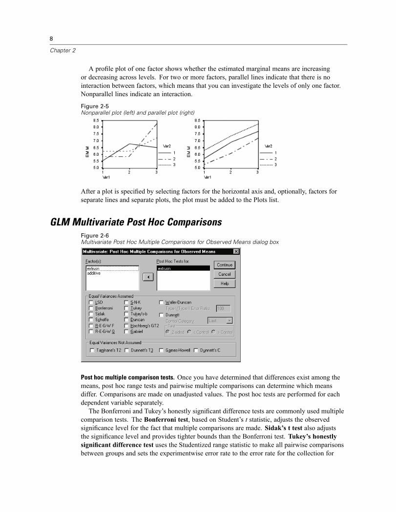
GLM Multivariate Post Hoc ComparisonsFigure 2-6Multivariate Post Hoc Multiple Comparisons for Observed Means dialog box

Post hoc multiple comparison tests. Once you have determined that differences exist among themeans, post hoc range tests and pairwise multiple comparisons can determine which meansdiffer. Comparisons are made on unadjusted values. The post hoc tests are performed for eachdependent variable separately.The Bonferroni and Tukey’s honestly significant difference tests are commonly used multiple

comparison tests. The Bonferroni test, based on Student’s t statistic, adjusts the observedsignificance level for the fact that multiple comparisons are made. Sidak’s t test also adjuststhe significance level and provides tighter bounds than the Bonferroni test. Tukey’s honestlysignificant difference test uses the Studentized range statistic to make all pairwise comparisonsbetween groups and sets the experimentwise error rate to the error rate for the collection for

9


all pairwise comparisons. When testing a large number of pairs of means, Tukey’s honestlysignificant difference test is more powerful than the Bonferroni test. For a small number ofpairs, Bonferroni is more powerful.Hochberg’s GT2 is similar to Tukey’s honestly significant difference test, but the Studentized

maximum modulus is used. Usually, Tukey’s test is more powerful. Gabriel’s pairwisecomparisons test also uses the Studentized maximum modulus and is generally more powerfulthan Hochberg’s GT2 when the cell sizes are unequal. Gabriel’s test may become liberal whenthe cell sizes vary greatly.Dunnett’s pairwise multiple comparison t test compares a set of treatments against a single

control mean. The last category is the default control category. Alternatively, you can choose thefirst category. You can also choose a two-sided or one-sided test. To test that the mean at anylevel (except the control category) of the factor is not equal to that of the control category, usea two-sided test. To test whether the mean at any level of the factor is smaller than that of thecontrol category, select < Control. Likewise, to test whether the mean at any level of the factor islarger than that of the control category, select > Control.Ryan, Einot, Gabriel, and Welsch (R-E-G-W) developed two multiple step-down range tests.

Multiple step-down procedures first test whether all means are equal. If all means are not equal,subsets of means are tested for equality. R-E-G-W F is based on an F test and R-E-G-W Q isbased on the Studentized range. These tests are more powerful than Duncan’s multiple range testand Student-Newman-Keuls (which are also multiple step-down procedures), but they are notrecommended for unequal cell sizes.When the variances are unequal, use Tamhane’s T2 (conservative pairwise comparisons test

based on a t test), Dunnett’s T3 (pairwise comparison test based on the Studentized maximummodulus), Games-Howell pairwise comparison test (sometimes liberal), or Dunnett’s C(pairwise comparison test based on the Studentized range).Duncan’s multiple range test, Student-Newman-Keuls (S-N-K), and Tukey’s b are range

tests that rank group means and compute a range value. These tests are not used as frequently asthe tests previously discussed.TheWaller-Duncan t test uses a Bayesian approach. This range test uses the harmonic mean

of the sample size when the sample sizes are unequal.The significance level of the Scheffé test is designed to allow all possible linear combinations

of group means to be tested, not just pairwise comparisons available in this feature. The resultis that the Scheffé test is often more conservative than other tests, which means that a largerdifference between means is required for significance.The least significant difference (LSD) pairwise multiple comparison test is equivalent to

multiple individual t tests between all pairs of groups. The disadvantage of this test is that noattempt is made to adjust the observed significance level for multiple comparisons.

Tests displayed. Pairwise comparisons are provided for LSD, Sidak, Bonferroni, Games-Howell,Tamhane’s T2 and T3, Dunnett’s C, and Dunnett’s T3. Homogeneous subsets for range tests areprovided for S-N-K, Tukey’s b, Duncan, R-E-G-W F, R-E-G-W Q, and Waller. Tukey’s honestlysignificant difference test, Hochberg’s GT2, Gabriel’s test, and Scheffé’s test are both multiplecomparison tests and range tests.

10

Chapter 2

GLM SaveFigure 2-7Save dialog box

You can save values predicted by the model, residuals, and related measures as new variables inthe Data Editor. Many of these variables can be used for examining assumptions about the data.To save the values for use in another SPSS session, you must save the current data file.

Predicted Values. The values that the model predicts for each case.Unstandardized. The value the model predicts for the dependent variable.Weighted. Weighted unstandardized predicted values. Available only if a WLS variablewas previously selected.Standard error. An estimate of the standard deviation of the average value of the dependentvariable for cases that have the same values of the independent variables.

Diagnostics. Measures to identify cases with unusual combinations of values for the independentvariables and cases that may have a large impact on the model.

Cook’s distance. A measure of how much the residuals of all cases would change if a particularcase were excluded from the calculation of the regression coefficients. A large Cook’s Dindicates that excluding a case from computation of the regression statistics changes thecoefficients substantially.Leverage values. Uncentered leverage values. The relative influence of each observation onthe model’s fit.

Residuals. An unstandardized residual is the actual value of the dependent variable minus thevalue predicted by the model. Standardized, Studentized, and deleted residuals are also available.If a WLS variable was chosen, weighted unstandardized residuals are available.

Unstandardized. The difference between an observed value and the value predicted by themodel.

11


Weighted. Weighted unstandardized residuals. Available only if a WLS variable waspreviously selected.Standardized. The residual divided by an estimate of its standard deviation. Standardizedresiduals, which are also known as Pearson residuals, have a mean of 0 and a standarddeviation of 1.Studentized. The residual divided by an estimate of its standard deviation that varies fromcase to case, depending on the distance of each case’s values on the independent variablesfrom the means of the independent variables.Deleted. The residual for a case when that case is excluded from the calculation of theregression coefficients. It is the difference between the value of the dependent variableand the adjusted predicted value.

Coefficient Statistics. Writes a variance-covariance matrix of the parameter estimates in themodel to a new dataset in the current session or an external SPSS-format data file. Also, for eachdependent variable, there will be a row of parameter estimates, a row of significance values forthe t statistics corresponding to the parameter estimates, and a row of residual degrees of freedom.For a multivariate model, there are similar rows for each dependent variable. You can use thismatrix file in other procedures that read an SPSS matrix file.

GLM Multivariate OptionsFigure 2-8Multivariate Options dialog box

Optional statistics are available from this dialog box. Statistics are calculated using a fixed-effectsmodel.

Estimated Marginal Means. Select the factors and interactions for which you want estimates ofthe population marginal means in the cells. These means are adjusted for the covariates, if any.Interactions are available only if you have specified a custom model.

12

Chapter 2

Compare main effects. Provides uncorrected pairwise comparisons among estimated marginalmeans for any main effect in the model, for both between- and within-subjects factors. Thisitem is available only if main effects are selected under the Display Means For list.Confidence interval adjustment. Select least significant difference (LSD), Bonferroni, orSidak adjustment to the confidence intervals and significance. This item is available only ifCompare main effects is selected.

Display. Select Descriptive statistics to produce observed means, standard deviations, and countsfor all of the dependent variables in all cells. Estimates of effect size gives a partial eta-squaredvalue for each effect and each parameter estimate. The eta-squared statistic describes theproportion of total variability attributable to a factor. Select Observed power to obtain the powerof the test when the alternative hypothesis is set based on the observed value. Select Parameter

estimates to produce the parameter estimates, standard errors, t tests, confidence intervals, and theobserved power for each test. You can display the hypothesis and error SSCP matrices and theResidual SSCP matrix plus Bartlett’s test of sphericity of the residual covariance matrix.

Homogeneity tests produces the Levene test of the homogeneity of variance for each dependentvariable across all level combinations of the between-subjects factors, for between-subjectsfactors only. Also, homogeneity tests include Box’s M test of the homogeneity of the covariancematrices of the dependent variables across all level combinations of the between-subjects factors.The spread-versus-level and residual plots options are useful for checking assumptions aboutthe data. This item is disabled if there are no factors. Select Residual plots to produce anobserved-by-predicted-by-standardized residuals plot for each dependent variable. These plotsare useful for investigating the assumption of equal variance. Select Lack of fit test to check if therelationship between the dependent variable and the independent variables can be adequatelydescribed by the model. General estimable function allows you to construct custom hypothesistests based on the general estimable function. Rows in any contrast coefficient matrix are linearcombinations of the general estimable function.

Significance level. You might want to adjust the significance level used in post hoc tests and theconfidence level used for constructing confidence intervals. The specified value is also used tocalculate the observed power for the test. When you specify a significance level, the associatedlevel of the confidence intervals is displayed in the dialog box.

GLM Command Additional Features

These features may apply to univariate, multivariate, or repeated measures analysis. The SPSScommand language also allows you to:

Specify nested effects in the design (using the DESIGN subcommand).Specify tests of effects versus a linear combination of effects or a value (using the TESTsubcommand).Specify multiple contrasts (using the CONTRAST subcommand).Include user-missing values (using the MISSING subcommand).Specify EPS criteria (using the CRITERIA subcommand).Construct a custom L matrix,M matrix, or K matrix (using the LMATRIX, MMATRIX, orKMATRIX subcommands).

13


For deviation or simple contrasts, specify an intermediate reference category (using theCONTRAST subcommand).Specify metrics for polynomial contrasts (using the CONTRAST subcommand).Specify error terms for post hoc comparisons (using the POSTHOC subcommand).Compute estimated marginal means for any factor or factor interaction among the factors inthe factor list (using the EMMEANS subcommand).Specify names for temporary variables (using the SAVE subcommand).Construct a correlation matrix data file (using the OUTFILE subcommand).Construct a matrix data file that contains statistics from the between-subjects ANOVA table(using the OUTFILE subcommand).Save the design matrix to a new data file (using the OUTFILE subcommand).

See the SPSS Command Syntax Reference for complete syntax information.

Chapter

3GLM Repeated Measures

The GLM Repeated Measures procedure provides analysis of variance when the samemeasurement is made several times on each subject or case. If between-subjects factors arespecified, they divide the population into groups. Using this general linear model procedure,you can test null hypotheses about the effects of both the between-subjects factors and thewithin-subjects factors. You can investigate interactions between factors as well as the effects ofindividual factors. In addition, the effects of constant covariates and covariate interactions withthe between-subjects factors can be included.In a doubly multivariate repeated measures design, the dependent variables represent

measurements of more than one variable for the different levels of the within-subjects factors.For example, you could have measured both pulse and respiration at three different times oneach subject.The GLM Repeated Measures procedure provides both univariate and multivariate analyses

for the repeated measures data. Both balanced and unbalanced models can be tested. A design isbalanced if each cell in the model contains the same number of cases. In a multivariate model,the sums of squares due to the effects in the model and error sums of squares are in matrixform rather than the scalar form found in univariate analysis. These matrices are called SSCP(sums-of-squares and cross-products) matrices. In addition to testing hypotheses, GLM RepeatedMeasures produces estimates of parameters.Commonly used a priori contrasts are available to perform hypothesis testing on

between-subjects factors. Additionally, after an overall F test has shown significance, you canuse post hoc tests to evaluate differences among specific means. Estimated marginal means giveestimates of predicted mean values for the cells in the model, and profile plots (interaction plots)of these means allow you to visualize some of the relationships easily.Residuals, predicted values, Cook’s distance, and leverage values can be saved as new

variables in your data file for checking assumptions. Also available are a residual SSCP matrix,which is a square matrix of sums of squares and cross-products of residuals, a residual covariancematrix, which is the residual SSCP matrix divided by the degrees of freedom of the residuals, andthe residual correlation matrix, which is the standardized form of the residual covariance matrix.WLS Weight allows you to specify a variable used to give observations different weights

for a weighted least-squares (WLS) analysis, perhaps to compensate for different precisionof measurement.

Example. Twelve students are assigned to a high- or low-anxiety group based on their scores onan anxiety-rating test. The anxiety rating is called a between-subjects factor because it divides thesubjects into groups. The students are each given four trials on a learning task, and the number oferrors for each trial is recorded. The errors for each trial are recorded in separate variables, and awithin-subjects factor (trial) is defined with four levels for the four trials. The trial effect is foundto be significant, while the trial-by-anxiety interaction is not significant.

14

15

GLM Repeated Measures

Methods. Type I, Type II, Type III, and Type IV sums of squares can be used to evaluate differenthypotheses. Type III is the default.

Statistics. Post hoc range tests and multiple comparisons (for between-subjects factors): leastsignificant difference, Bonferroni, Sidak, Scheffé, Ryan-Einot-Gabriel-Welsch multiple F,Ryan-Einot-Gabriel-Welsch multiple range, Student-Newman-Keuls, Tukey’s honestly significantdifference, Tukey’s b, Duncan, Hochberg’s GT2, Gabriel, Waller Duncan t test, Dunnett(one-sided and two-sided), Tamhane’s T2, Dunnett’s T3, Games-Howell, and Dunnett’s C.Descriptive statistics: observed means, standard deviations, and counts for all of the dependentvariables in all cells; the Levene test for homogeneity of variance; Box’s M; and Mauchly’stest of sphericity.

Plots. Spread-versus-level, residual, and profile (interaction).

Data. The dependent variables should be quantitative. Between-subjects factors divide the sampleinto discrete subgroups, such as male and female. These factors are categorical and can havenumeric values or string values of up to eight characters. Within-subjects factors are defined inthe Repeated Measures Define Factor(s) dialog box. Covariates are quantitative variables thatare related to the dependent variable. For a repeated measures analysis, these should remainconstant at each level of a within-subjects variable.The data file should contain a set of variables for each group of measurements on the

subjects. The set has one variable for each repetition of the measurement within the group. Awithin-subjects factor is defined for the group with the number of levels equal to the numberof repetitions. For example, measurements of weight could be taken on different days. Ifmeasurements of the same property were taken on five days, the within-subjects factor couldbe specified as day with five levels.For multiple within-subjects factors, the number of measurements for each subject is equal to

the product of the number of levels of each factor. For example, if measurements were takenat three different times each day for four days, the total number of measurements is 12 for eachsubject. The within-subjects factors could be specified as day(4) and time(3).

Assumptions. A repeated measures analysis can be approached in two ways, univariate andmultivariate.The univariate approach (also known as the split-plot or mixed-model approach) considers the

dependent variables as responses to the levels of within-subjects factors. The measurements on asubject should be a sample from a multivariate normal distribution, and the variance-covariancematrices are the same across the cells formed by the between-subjects effects. Certainassumptions are made on the variance-covariance matrix of the dependent variables. The validityof the F statistic used in the univariate approach can be assured if the variance-covariance matrixis circular in form (Huynh and Mandeville, 1979).To test this assumption, Mauchly’s test of sphericity can be used, which performs a test of

sphericity on the variance-covariance matrix of an orthonormalized transformed dependentvariable. Mauchly’s test is automatically displayed for a repeated measures analysis. For smallsample sizes, this test is not very powerful. For large sample sizes, the test may be significanteven when the impact of the departure on the results is small. If the significance of the test islarge, the hypothesis of sphericity can be assumed. However, if the significance is small and thesphericity assumption appears to be violated, an adjustment to the numerator and denominatordegrees of freedom can be made in order to validate the univariate F statistic. Three estimates ofthis adjustment, which is called epsilon, are available in the GLM Repeated Measures procedure.

16

Chapter 3

Both the numerator and denominator degrees of freedom must be multiplied by epsilon, and thesignificance of the F ratio must be evaluated with the new degrees of freedom.The multivariate approach considers the measurements on a subject to be a sample from a

multivariate normal distribution, and the variance-covariance matrices are the same across thecells formed by the between-subjects effects. To test whether the variance-covariance matricesacross the cells are the same, Box’s M test can be used.

Related procedures. Use the Explore procedure to examine the data before doing an analysisof variance. If there are not repeated measurements on each subject, use GLM Univariate orGLM Multivariate. If there are only two measurements for each subject (for example, pre-testand post-test), and there are no between-subjects factors, you can use the Paired-Samples TTest procedure.

Obtaining GLM Repeated Measures


General Linear ModelRepeated Measures...

Figure 3-1Repeated Measures Define Factor(s) dialog box

E Type a within-subject factor name and its number of levels.

E Click Add.

E Repeat these steps for each within-subjects factor.

To define measure factors for a doubly multivariate repeated measures design:

E Type the measure name.

E Click Add.

After defining all of your factors and measures:

E Click Define.

17


Figure 3-2Repeated Measures dialog box

E Select a dependent variable that corresponds to each combination of within-subjects factors(and optionally, measures) on the list.

To change positions of the variables, use the up and down arrows.To make changes to the within-subjects factors, you can reopen the Repeated Measures

Define Factor(s) dialog box without closing the main dialog box. Optionally, you can specifybetween-subjects factor(s) and covariates.

GLM Repeated Measures Define FactorsGLM Repeated Measures analyzes groups of related dependent variables that represent differentmeasurements of the same attribute. This dialog box lets you define one or more within-subjectsfactors for use in GLM Repeated Measures. See Figure 3-1 on p. 16. Note that the order inwhich you specify within-subjects factors is important. Each factor constitutes a level withinthe previous factor.To use Repeated Measures, you must set up your data correctly. You must define

within-subjects factors in this dialog box. Notice that these factors are not existing variables inyour data but rather factors that you define here.

Example. In a weight-loss study, suppose the weights of several people are measured each weekfor five weeks. In the data file, each person is a subject or case. The weights for the weeks arerecorded in the variables weight1, weight2, and so on. The gender of each person is recordedin another variable. The weights, measured for each subject repeatedly, can be grouped bydefining a within-subjects factor. The factor could be called week, defined to have five levels.In the main dialog box, the variables weight1, ..., weight5 are used to assign the five levels ofweek. The variable in the data file that groups males and females (gender) can be specified as abetween-subjects factor to study the differences between males and females.

18

Chapter 3

Measures. If subjects were tested on more than one measure at each time, define the measures.For example, the pulse and respiration rate could be measured on each subject every day for aweek. These measures do not exist as variables in the data file but are defined here. A model withmore than one measure is sometimes called a doubly multivariate repeated measures model.

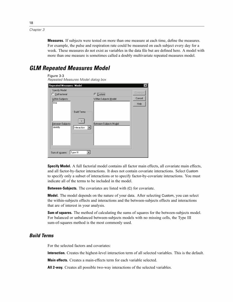
GLM Repeated Measures ModelFigure 3-3Repeated Measures Model dialog box



Between-Subjects. The covariates are listed with (C) for covariate.

Model. The model depends on the nature of your data. After selecting Custom, you can selectthe within-subjects effects and interactions and the between-subjects effects and interactionsthat are of interest in your analysis.

Sum of squares. The method of calculating the sums of squares for the between-subjects model.For balanced or unbalanced between-subjects models with no missing cells, the Type IIIsum-of-squares method is the most commonly used.

Build Terms





19





Sum of Squares


Type I. This method is also known as the hierarchical decomposition of the sum-of-squaresmethod. Each term is adjusted for only the term that precedes it in the model. Type I sumsof squares are commonly used for:


Type II. This method calculates the sums of squares of an effect in the model adjusted for all other“appropriate” effects. An appropriate effect is one that corresponds to all effects that do notcontain the effect being examined. The Type II sum-of-squares method is commonly used for:

A balanced ANOVA model.Any model that has main factor effects only.Any regression model.A purely nested design. (This form of nesting can be specified by using syntax.)


Any models listed in Type I and Type II.Any balanced or unbalanced model with no empty cells.

20

Chapter 3

Type IV. This method is designed for a situation in which there are missing cells. For any effect Fin the design, if F is not contained in any other effect, then Type IV = Type III = Type II. When Fis contained in other effects, Type IV distributes the contrasts being made among the parameters inF to all higher-level effects equitably. The Type IV sum-of-squares method is commonly used for:

Any models listed in Type I and Type II.Any balanced model or unbalanced model with empty cells.

GLM Repeated Measures ContrastsFigure 3-4Repeated Measures Contrasts dialog box

Contrasts are used to test for differences among the levels of a between-subjects factor. You canspecify a contrast for each between-subjects factor in the model. Contrasts represent linearcombinations of the parameters.Hypothesis testing is based on the null hypothesis LBM=0, where L is the contrast coefficients

matrix, B is the parameter vector, andM is the average matrix that corresponds to the averagetransformation for the dependent variable. You can display this transformation matrix by selectingTransformation matrix in the Repeated Measures Options dialog box. For example, if there are fourdependent variables, a within-subjects factor of four levels, and polynomial contrasts (the default)are used for within-subjects factors, theM matrix will be (0.5 0.5 0.5 0.5)’. When a contrast isspecified, SPSS creates an L matrix such that the columns corresponding to the between-subjectsfactor match the contrast. The remaining columns are adjusted so that the L matrix is estimable.Available contrasts are deviation, simple, difference, Helmert, repeated, and polynomial. For

deviation contrasts and simple contrasts, you can choose whether the reference category is thelast or first category.

Contrast Types

Deviation. Compares the mean of each level (except a reference category) to the mean of all of thelevels (grand mean). The levels of the factor can be in any order.

Simple. Compares the mean of each level to the mean of a specified level. This type of contrast isuseful when there is a control group. You can choose the first or last category as the reference.

Difference. Compares the mean of each level (except the first) to the mean of previous levels.(Sometimes called reverse Helmert contrasts.)

21


Helmert. Compares the mean of each level of the factor (except the last) to the mean of subsequentlevels.

Repeated. Compares the mean of each level (except the last) to the mean of the subsequent level.

Polynomial. Compares the linear effect, quadratic effect, cubic effect, and so on. The first degreeof freedom contains the linear effect across all categories; the second degree of freedom, thequadratic effect; and so on. These contrasts are often used to estimate polynomial trends.

GLM Repeated Measures Profile PlotsFigure 3-5Repeated Measures Profile Plots dialog box

Profile plots (interaction plots) are useful for comparing marginal means in your model. A profileplot is a line plot in which each point indicates the estimated marginal mean of a dependentvariable (adjusted for any covariates) at one level of a factor. The levels of a second factor can beused to make separate lines. Each level in a third factor can be used to create a separate plot.All factors are available for plots. Profile plots are created for each dependent variable. Bothbetween-subjects factors and within-subjects factors can be used in profile plots.A profile plot of one factor shows whether the estimated marginal means are increasing

or decreasing across levels. For two or more factors, parallel lines indicate that there is nointeraction between factors, which means that you can investigate the levels of only one factor.Nonparallel lines indicate an interaction.

Figure 3-6Nonparallel plot (left) and parallel plot (right)

22

Chapter 3

After a plot is specified by selecting factors for the horizontal axis and, optionally, factors forseparate lines and separate plots, the plot must be added to the Plots list.

GLM Repeated Measures Post Hoc ComparisonsFigure 3-7Repeated Measures Post Hoc Multiple Comparisons for Observed Means dialog box

Post hoc multiple comparison tests. Once you have determined that differences exist among themeans, post hoc range tests and pairwise multiple comparisons can determine which meansdiffer. Comparisons are made on unadjusted values. These tests are not available if there areno between-subjects factors, and the post hoc multiple comparison tests are performed for theaverage across the levels of the within-subjects factors.The Bonferroni and Tukey’s honestly significant difference tests are commonly used multiple

comparison tests. The Bonferroni test, based on Student’s t statistic, adjusts the observedsignificance level for the fact that multiple comparisons are made. Sidak’s t test also adjuststhe significance level and provides tighter bounds than the Bonferroni test. Tukey’s honestlysignificant difference test uses the Studentized range statistic to make all pairwise comparisonsbetween groups and sets the experimentwise error rate to the error rate for the collection forall pairwise comparisons. When testing a large number of pairs of means, Tukey’s honestlysignificant difference test is more powerful than the Bonferroni test. For a small number ofpairs, Bonferroni is more powerful.Hochberg’s GT2 is similar to Tukey’s honestly significant difference test, but the Studentized

maximum modulus is used. Usually, Tukey’s test is more powerful. Gabriel’s pairwisecomparisons test also uses the Studentized maximum modulus and is generally more powerfulthan Hochberg’s GT2 when the cell sizes are unequal. Gabriel’s test may become liberal whenthe cell sizes vary greatly.Dunnett’s pairwise multiple comparison t test compares a set of treatments against a single

control mean. The last category is the default control category. Alternatively, you can choose thefirst category. You can also choose a two-sided or one-sided test. To test that the mean at anylevel (except the control category) of the factor is not equal to that of the control category, usea two-sided test. To test whether the mean at any level of the factor is smaller than that of the

23


control category, select < Control. Likewise, to test whether the mean at any level of the factor islarger than that of the control category, select > Control.Ryan, Einot, Gabriel, and Welsch (R-E-G-W) developed two multiple step-down range tests.

Multiple step-down procedures first test whether all means are equal. If all means are not equal,subsets of means are tested for equality. R-E-G-W F is based on an F test and R-E-G-W Q isbased on the Studentized range. These tests are more powerful than Duncan’s multiple range testand Student-Newman-Keuls (which are also multiple step-down procedures), but they are notrecommended for unequal cell sizes.When the variances are unequal, use Tamhane’s T2 (conservative pairwise comparisons test

based on a t test), Dunnett’s T3 (pairwise comparison test based on the Studentized maximummodulus), Games-Howell pairwise comparison test (sometimes liberal), or Dunnett’s C(pairwise comparison test based on the Studentized range).Duncan’s multiple range test, Student-Newman-Keuls (S-N-K), and Tukey’s b are range

tests that rank group means and compute a range value. These tests are not used as frequently asthe tests previously discussed.TheWaller-Duncan t test uses a Bayesian approach. This range test uses the harmonic mean

of the sample size when the sample sizes are unequal.The significance level of the Scheffé test is designed to allow all possible linear combinations

of group means to be tested, not just pairwise comparisons available in this feature. The resultis that the Scheffé test is often more conservative than other tests, which means that a largerdifference between means is required for significance.The least significant difference (LSD) pairwise multiple comparison test is equivalent to

multiple individual t tests between all pairs of groups. The disadvantage of this test is that noattempt is made to adjust the observed significance level for multiple comparisons.

Tests displayed. Pairwise comparisons are provided for LSD, Sidak, Bonferroni, Games-Howell,Tamhane’s T2 and T3, Dunnett’s C, and Dunnett’s T3. Homogeneous subsets for range tests areprovided for S-N-K, Tukey’s b, Duncan, R-E-G-W F, R-E-G-W Q, and Waller. Tukey’s honestlysignificant difference test, Hochberg’s GT2, Gabriel’s test, and Scheffé’s test are both multiplecomparison tests and range tests.

24

Chapter 3

GLM Repeated Measures SaveFigure 3-8Repeated Measures Save dialog box

You can save values predicted by the model, residuals, and related measures as new variables inthe Data Editor. Many of these variables can be used for examining assumptions about the data.To save the values for use in another SPSS session, you must save the current data file.

Predicted Values. The values that the model predicts for each case.Unstandardized. The value the model predicts for the dependent variable.Standard error. An estimate of the standard deviation of the average value of the dependentvariable for cases that have the same values of the independent variables.

Diagnostics. Measures to identify cases with unusual combinations of values for the independentvariables and cases that may have a large impact on the model. Available are Cook’s distance anduncentered leverage values.

Cook’s distance. A measure of how much the residuals of all cases would change if a particularcase were excluded from the calculation of the regression coefficients. A large Cook’s Dindicates that excluding a case from computation of the regression statistics changes thecoefficients substantially.Leverage values. Uncentered leverage values. The relative influence of each observation onthe model’s fit.

Residuals. An unstandardized residual is the actual value of the dependent variable minus thevalue predicted by the model. Standardized, Studentized, and deleted residuals are also available.

Unstandardized. The difference between an observed value and the value predicted by themodel.Standardized. The residual divided by an estimate of its standard deviation. Standardizedresiduals, which are also known as Pearson residuals, have a mean of 0 and a standarddeviation of 1.

25


Studentized. The residual divided by an estimate of its standard deviation that varies fromcase to case, depending on the distance of each case’s values on the independent variablesfrom the means of the independent variables.Deleted. The residual for a case when that case is excluded from the calculation of theregression coefficients. It is the difference between the value of the dependent variableand the adjusted predicted value.

Coefficient Statistics. Saves a variance-covariance matrix of the parameter estimates to a datasetor a data file. Also, for each dependent variable, there will be a row of parameter estimates, a rowof significance values for the t statistics corresponding to the parameter estimates, and a row ofresidual degrees of freedom. For a multivariate model, there are similar rows for each dependentvariable. You can use this matrix data in other procedures that read an SPSS matrix file. Datasetsare available for subsequent use in the same session but are not saved as files unless explicitlysaved prior to the end of the session. Dataset names must conform to SPSS variable naming rules.

GLM Repeated Measures OptionsFigure 3-9Repeated Measures Options dialog box

Optional statistics are available from this dialog box. Statistics are calculated using a fixed-effectsmodel.

Estimated Marginal Means. Select the factors and interactions for which you want estimates of thepopulation marginal means in the cells. These means are adjusted for the covariates, if any. Bothwithin-subjects and between-subjects factors can be selected.

26

Chapter 3

Compare main effects. Provides uncorrected pairwise comparisons among estimated marginalmeans for any main effect in the model, for both between- and within-subjects factors. Thisitem is available only if main effects are selected under the Display Means For list.Confidence interval adjustment. Select least significant difference (LSD), Bonferroni, orSidak adjustment to the confidence intervals and significance. This item is available only ifCompare main effects is selected.

Display. Select Descriptive statistics to produce observed means, standard deviations, and countsfor all of the dependent variables in all cells. Estimates of effect size gives a partial eta-squaredvalue for each effect and each parameter estimate. The eta-squared statistic describes theproportion of total variability attributable to a factor. Select Observed power to obtain the powerof the test when the alternative hypothesis is set based on the observed value. Select Parameter

estimates to produce the parameter estimates, standard errors, t tests, confidence intervals, and theobserved power for each test. You can display the hypothesis and error SSCP matrices and theResidual SSCP matrix plus Bartlett’s test of sphericity of the residual covariance matrix.

Homogeneity tests produces the Levene test of the homogeneity of variance for each dependentvariable across all level combinations of the between-subjects factors, for between-subjectsfactors only. Also, homogeneity tests include Box’s M test of the homogeneity of the covariancematrices of the dependent variables across all level combinations of the between-subjects factors.The spread-versus-level and residual plots options are useful for checking assumptions aboutthe data. This item is disabled if there are no factors. Select Residual plots to produce anobserved-by-predicted-by-standardized residuals plot for each dependent variable. These plotsare useful for investigating the assumption of equal variance. Select Lack of fit test to check if therelationship between the dependent variable and the independent variables can be adequatelydescribed by the model. General estimable function allows you to construct custom hypothesistests based on the general estimable function. Rows in any contrast coefficient matrix are linearcombinations of the general estimable function.

Significance level. You might want to adjust the significance level used in post hoc tests and theconfidence level used for constructing confidence intervals. The specified value is also used tocalculate the observed power for the test. When you specify a significance level, the associatedlevel of the confidence intervals is displayed in the dialog box.

GLM Command Additional Features

These features may apply to univariate, multivariate, or repeated measures analysis. The SPSScommand language also allows you to:

Specify nested effects in the design (using the DESIGN subcommand).Specify tests of effects versus a linear combination of effects or a value (using the TESTsubcommand).Specify multiple contrasts (using the CONTRAST subcommand).Include user-missing values (using the MISSING subcommand).Specify EPS criteria (using the CRITERIA subcommand).Construct a custom L matrix,M matrix, or K matrix (using the LMATRIX, MMATRIX, andKMATRIX subcommands).

27


For deviation or simple contrasts, specify an intermediate reference category (using theCONTRAST subcommand).Specify metrics for polynomial contrasts (using the CONTRAST subcommand).Specify error terms for post hoc comparisons (using the POSTHOC subcommand).Compute estimated marginal means for any factor or factor interaction among the factors inthe factor list (using the EMMEANS subcommand).Specify names for temporary variables (using the SAVE subcommand).Construct a correlation matrix data file (using the OUTFILE subcommand).Construct a matrix data file that contains statistics from the between-subjects ANOVA table(using the OUTFILE subcommand).Save the design matrix to a new data file (using the OUTFILE subcommand).


Chapter

4Variance Components Analysis

The Variance Components procedure, for mixed-effects models, estimates the contribution ofeach random effect to the variance of the dependent variable. This procedure is particularlyinteresting for analysis of mixed models such as split plot, univariate repeated measures, andrandom block designs. By calculating variance components, you can determine where to focusattention in order to reduce the variance.Four different methods are available for estimating the variance components: minimum norm

quadratic unbiased estimator (MINQUE), analysis of variance (ANOVA), maximum likelihood(ML), and restricted maximum likelihood (REML). Various specifications are available forthe different methods.Default output for all methods includes variance component estimates. If the ML method

or the REML method is used, an asymptotic covariance matrix table is also displayed. Otheravailable output includes an ANOVA table and expected mean squares for the ANOVA method,and an iteration history for the ML and REML methods. The Variance Components procedure isfully compatible with the GLM Univariate procedure.WLS Weight allows you to specify a variable used to give observations different weights for a

weighted analysis, perhaps to compensate for different precision of measurement.

Example. At an agriculture school, weight gains for pigs in six different litters are measuredafter one month. The litter variable is a random factor with six levels. (The six litters studiedare a random sample from a large population of pig litters.) The investigator finds out that thevariance in weight gain is attributable to the difference in litters much more than to the differencein pigs within a litter.

Data. The dependent variable is quantitative. Factors are categorical. They can have numericvalues or string values of up to eight characters. At least one of the factors must be random. Thatis, the levels of the factor must be a random sample of possible levels. Covariates are quantitativevariables that are related to the dependent variable.

Assumptions. All methods assume that model parameters of a random effect have zero meansand finite constant variances and are mutually uncorrelated. Model parameters from differentrandom effects are also uncorrelated.The residual term also has a zero mean and finite constant variance. It is uncorrelated with

model parameters of any random effect. Residual terms from different observations are assumedto be uncorrelated.Based on these assumptions, observations from the same level of a random factor are

correlated. This fact distinguishes a variance component model from a general linear model.ANOVA and MINQUE do not require normality assumptions. They are both robust to

moderate departures from the normality assumption.ML and REML require the model parameter and the residual term to be normally distributed.

28

29

Variance Components Analysis

Related procedures. Use the Explore procedure to examine the data before doing variancecomponents analysis. For hypothesis testing, use GLM Univariate, GLM Multivariate, andGLM Repeated Measures.

Obtaining Variance Components Tables


General Linear ModelVariance Components...

Figure 4-1Variance Components dialog box

E Select a dependent variable.

E Select variables for Fixed Factor(s), Random Factor(s), and Covariate(s), as appropriate for yourdata. For specifying a weight variable, use WLS Weight.

30

Chapter 4

Variance Components ModelFigure 4-2Variance Components Model dialog box



Factors and Covariates. The factors and covariates are listed with (F) for a fixed factor, (R) for arandom factor, and (C) for a covariate.

Model. The model depends on the nature of your data. After selecting Custom, you can selectthe main effects and interactions that are of interest in your analysis. The model must contain arandom factor.

Include intercept in model. Usually the intercept is included in the model. If you can assume thatthe data pass through the origin, you can exclude the intercept.

Build Terms








31


Variance Components OptionsFigure 4-3Variance Components Options dialog box

Method. You can choose one of four methods to estimate the variance components.MINQUE (minimum norm quadratic unbiased estimator) produces estimates that are invariantwith respect to the fixed effects. If the data are normally distributed and the estimates arecorrect, this method produces the least variance among all unbiased estimators. You canchoose a method for random-effect prior weights.ANOVA (analysis of variance) computes unbiased estimates using either the Type I or Type IIIsums of squares for each effect. The ANOVA method sometimes produces negative varianceestimates, which can indicate an incorrect model, an inappropriate estimation method, or aneed for more data.Maximum likelihood (ML) produces estimates that would be most consistent with thedata actually observed, using iterations. These estimates can be biased. This method isasymptotically normal. ML and REML estimates are invariant under translation. Thismethod does not take into account the degrees of freedom used to estimate the fixed effects.Restricted maximum likelihood (REML) estimates reduce the ANOVA estimates for many(if not all) cases of balanced data. Because this method is adjusted for the fixed effects, itshould have smaller standard errors than the ML method. This method takes into accountthe degrees of freedom used to estimate the fixed effects.

Random Effect Priors. Uniform implies that all random effects and the residual term have an equalimpact on the observations. The Zero scheme is equivalent to assuming zero random-effectvariances. Available only for the MINQUE method.

Sum of Squares. Type I sums of squares are used for the hierarchical model, which is often used invariance component literature. If you choose Type III, the default in GLM, the variance estimatescan be used in GLM Univariate for hypothesis testing with Type III sums of squares. Availableonly for the ANOVA method.

Criteria. You can specify the convergence criterion and the maximum number of iterations.Available only for the ML or REML methods.

32

Chapter 4

Display. For the ANOVA method, you can choose to display sums of squares and expectedmean squares. If you selected Maximum likelihood or Restricted maximum likelihood, you candisplay a history of the iterations.

Sum of Squares (Variance Components)

For the model, you can choose a type of sum of squares. Type III is the most commonly usedand is the default.

Type I. This method is also known as the hierarchical decomposition of the sum-of-squaresmethod. Each term is adjusted for only the term that precedes it in the model. The Type Isum-of-squares method is commonly used for:


Type III. The default. This method calculates the sums of squares of an effect in the design asthe sums of squares adjusted for any other effects that do not contain it and orthogonal to anyeffects (if any) that contain it. The Type III sums of squares have one major advantage in thatthey are invariant with respect to the cell frequencies as long as the general form of estimabilityremains constant. Therefore, this type is often considered useful for an unbalanced model withno missing cells. In a factorial design with no missing cells, this method is equivalent to theYates’ weighted-squares-of-means technique. The Type III sum-of-squares method is commonlyused for:

Any models listed in Type I.Any balanced or unbalanced model with no empty cells.

33


Variance Components Save to New FileFigure 4-4Variance Components Save to New File dialog box

You can save some results of this procedure to a new SPSS data file.

Variance component estimates. Saves estimates of the variance components and estimate labelsto a data file or dataset. These can be used in calculating more statistics or in further analysisin the GLM procedures. For example, you can use them to calculate confidence intervals ortest hypotheses.

Component covariation. Saves a variance-covariance matrix or a correlation matrix to a data file ordataset. Available only if Maximum likelihood or Restricted maximum likelihood has been specified.

Destination for created values. Allows you to specify a dataset name or external filename for thefile containing the variance component estimates and/or the matrix. Datasets are available forsubsequent use in the same session but are not saved as files unless explicitly saved prior to theend of the session. Dataset names must conform to SPSS variable naming rules.

You can use the MATRIX command to extract the data you need from the data file and thencompute confidence intervals or perform tests.

VARCOMP Command Additional Features

The SPSS command language also allows you to:Specify nested effects in the design (using the DESIGN subcommand).Include user-missing values (using the MISSING subcommand).Specify EPS criteria (using the CRITERIA subcommand).


Chapter

5Linear Mixed Models

The Linear Mixed Models procedure expands the general linear model so that the data arepermitted to exhibit correlated and nonconstant variability. The mixed linear model, therefore,provides the flexibility of modeling not only the means of the data but their variances andcovariances as well.The Linear Mixed Models procedure is also a flexible tool for fitting other models that can

be formulated as mixed linear models. Such models include multilevel models, hierarchicallinear models, and random coefficient models.

Example. A grocery store chain is interested in the effects of various coupons on customerspending. Taking a random sample of their regular customers, they follow the spending of eachcustomer for 10 weeks. In each week, a different coupon is mailed to the customers. LinearMixed Models is used to estimate the effect of different coupons on spending while adjusting forcorrelation due to repeated observations on each subject over the 10 weeks.

Methods. Maximum likelihood (ML) and restricted maximum likelihood (REML) estimation.

Statistics. Descriptive statistics: sample sizes, means, and standard deviations of the dependentvariable and covariates for each distinct level combination of the factors. Factor-levelinformation: sorted values of the levels of each factor and their frequencies. Also, parameterestimates and confidence intervals for fixed effects, Wald tests and confidence intervals forparameters of covariance matrices. Type I and Type III sums of squares can be used to evaluatedifferent hypotheses. Type III is the default.

Data. The dependent variable should be quantitative. Factors should be categorical and can havenumeric values or string values. Covariates and the weight variable should be quantitative.Subjects and repeated variables may be of any type.

Assumptions. The dependent variable is assumed to be linearly related to the fixed factors, randomfactors, and covariates. The fixed effects model the mean of the dependent variable. The randomeffects model the covariance structure of the dependent variable. Multiple random effects areconsidered independent of each other, and separate covariance matrices will be computed foreach; however, model terms specified on the same random effect can be correlated. The repeatedmeasures model the covariance structure of the residuals. The dependent variable is also assumedto come from a normal distribution.

Related procedures. Use the Explore procedure to examine the data before running an analysis. Ifyou do not suspect there to be correlated or nonconstant variability, you can alternatively use theGLM Univariate or GLM Repeated Measures procedure. You can alternatively use the VarianceComponents Analysis procedure if the random effects have a variance components covariancestructure and there are no repeated measures.

34

35

Linear Mixed Models

Obtaining a Linear Mixed Models Analysis


Mixed ModelsLinear...

Figure 5-1Linear Mixed Models Specify Subjects and Repeated Variables dialog box

E Optionally, select one or more subjects variables.

E Optionally, select one or more repeated variables.

E Optionally, select a residual covariance structure.

E Click Continue.

36

Chapter 5

Figure 5-2Linear Mixed Models dialog box

E Select a dependent variable.

E Select at least one factor or covariate.

E Click Fixed or Random and specify at least a fixed-effects or random-effects model.

Optionally, select a weighting variable.

Linear Mixed Models Select Subjects/Repeated Variables

This dialog box allows you to select variables that define subjects and repeated observations andto choose a covariance structure for the residuals. See Figure 5-1 on p. 35.

Subjects. A subject is an observational unit that can be considered independent of other subjects.For example, the blood pressure readings from a patient in a medical study can be consideredindependent of the readings from other patients. Defining subjects becomes particularly importantwhen there are repeated measurements per subject and you want to model the correlation betweenthese observations. For example, you might expect that blood pressure readings from a singlepatient during consecutive visits to the doctor are correlated.Subjects can also be defined by the factor-level combination of multiple variables; for example,

you can specify Gender and Age category as subject variables to model the belief that males overthe age of 65 are similar to each other but independent of males under 65 and females.All of the variables specified in the Subjects list are used to define subjects for the residual

covariance structure. You can use some or all of the variables to define subjects for therandom-effects covariance structure.

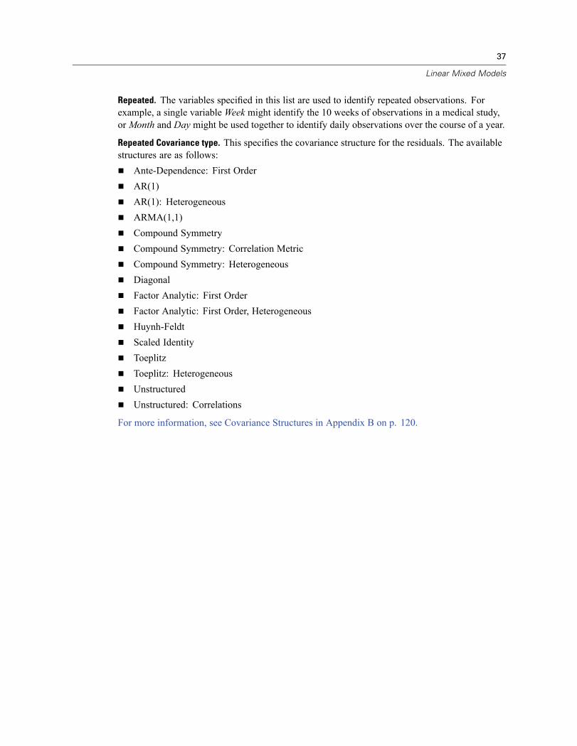
37

Linear Mixed Models

Repeated. The variables specified in this list are used to identify repeated observations. Forexample, a single variable Week might identify the 10 weeks of observations in a medical study,orMonth and Day might be used together to identify daily observations over the course of a year.

Repeated Covariance type. This specifies the covariance structure for the residuals. The availablestructures are as follows:

Ante-Dependence: First OrderAR(1)AR(1): HeterogeneousARMA(1,1)Compound SymmetryCompound Symmetry: Correlation MetricCompound Symmetry: HeterogeneousDiagonalFactor Analytic: First OrderFactor Analytic: First Order, HeterogeneousHuynh-FeldtScaled IdentityToeplitzToeplitz: HeterogeneousUnstructuredUnstructured: Correlations

For more information, see Covariance Structures in Appendix B on p. 120.

38

Chapter 5

Linear Mixed Models Fixed EffectsFigure 5-3Linear Mixed Models Fixed Effects dialog box

Fixed Effects. There is no default model, so you must explicitly specify the fixed effects.Alternatively, you can build nested or non-nested terms.

Include Intercept. The intercept is usually included in the model. If you can assume the data passthrough the origin, you can exclude the intercept.

Sum of squares. The method of calculating the sums of squares. For models with no missing cells,the Type III method is most commonly used.

Build Non-Nested Terms


Factorial. Creates all possible interactions and main effects of the selected variables. This isthe default.

Interaction. Creates the highest-level interaction term of all selected variables.

Main Effects. Creates a main-effects term for each variable selected.

All 2-Way. Creates all possible two-way interactions of the selected variables.

All 3-Way. Creates all possible three-way interactions of the selected variables.

All 4-Way. Creates all possible four-way interactions of the selected variables.

All 5-Way. Creates all possible five-way interactions of the selected variables.

39

Linear Mixed Models

Build Nested Terms

You can build nested terms for your model in this procedure. Nested terms are useful for modelingthe effect of a factor or covariate whose values do not interact with the levels of another factor.For example, a grocery store chain may follow the spending of their customers at several storelocations. Since each customer frequents only one of those locations, the Customer effect can besaid to be nested within the Store location effect.Additionally, you can include interaction effects or add multiple levels of nesting to the nested

term.

Limitations. Nested terms have the following restrictions:All factors within an interaction must be unique. Thus, if A is a factor, then specifying A*Ais invalid.All factors within a nested effect must be unique. Thus, if A is a factor, then specifyingA(A) is invalid.No effect can be nested within a covariate. Thus, if A is a factor and X is a covariate, thenspecifying A(X) is invalid.

Sum of Squares


Type I. This method is also known as the hierarchical decomposition of the sum-of-squaresmethod. Each term is adjusted only for the term that precedes it in the model. Type I sumsof squares are commonly used for:



Any models listed in Type I.Any balanced or unbalanced model with no empty cells.

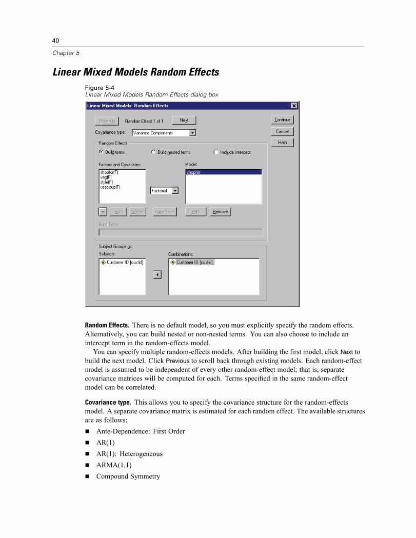
40

Chapter 5

Linear Mixed Models Random EffectsFigure 5-4Linear Mixed Models Random Effects dialog box

Random Effects. There is no default model, so you must explicitly specify the random effects.Alternatively, you can build nested or non-nested terms. You can also choose to include anintercept term in the random-effects model.You can specify multiple random-effects models. After building the first model, click Next to

build the next model. Click Previous to scroll back through existing models. Each random-effectmodel is assumed to be independent of every other random-effect model; that is, separatecovariance matrices will be computed for each. Terms specified in the same random-effectmodel can be correlated.

Covariance type. This allows you to specify the covariance structure for the random-effectsmodel. A separate covariance matrix is estimated for each random effect. The available structuresare as follows:

Ante-Dependence: First OrderAR(1)AR(1): HeterogeneousARMA(1,1)Compound Symmetry

41

Linear Mixed Models

Compound Symmetry: Correlation MetricCompound Symmetry: HeterogeneousDiagonalFactor Analytic: First OrderFactor Analytic: First Order, HeterogeneousHuynh-FeldtScaled IdentityToeplitzToeplitz: HeterogeneousUnstructuredUnstructured: Correlation MetricVariance Components

For more information, see Covariance Structures in Appendix B on p. 120.

Subject Groupings. The variables listed are those that you selected as subject variables in theSelect Subjects/Repeated Variables dialog box. Choose some or all of these in order to define thesubjects for the random-effects model.

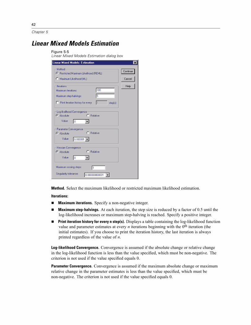
42

Chapter 5

Linear Mixed Models EstimationFigure 5-5Linear Mixed Models Estimation dialog box

Method. Select the maximum likelihood or restricted maximum likelihood estimation.

Iterations:

Maximum iterations. Specify a non-negative integer.Maximum step-halvings. At each iteration, the step size is reduced by a factor of 0.5 until thelog-likelihood increases or maximum step-halving is reached. Specify a positive integer.Print iteration history for every n step(s). Displays a table containing the log-likelihood functionvalue and parameter estimates at every n iterations beginning with the 0th iteration (theinitial estimates). If you choose to print the iteration history, the last iteration is alwaysprinted regardless of the value of n.

Log-likelihood Convergence. Convergence is assumed if the absolute change or relative changein the log-likelihood function is less than the value specified, which must be non-negative. Thecriterion is not used if the value specified equals 0.

Parameter Convergence. Convergence is assumed if the maximum absolute change or maximumrelative change in the parameter estimates is less than the value specified, which must benon-negative. The criterion is not used if the value specified equals 0.

43

Linear Mixed Models

Hessian Convergence. For the Absolute specification, convergence is assumed if a statistic basedon the Hessian is less than the value specified. For the Relative specification, convergence isassumed if the statistic is less than the product of the value specified and the absolute value of thelog-likelihood. The criterion is not used if the value specified equals 0.

Maximum scoring steps. Requests to use the Fisher scoring algorithm up to iteration number n.Specify a positive integer.

Singularity tolerance. This is the value used as tolerance in checking singularity. Specify apositive value.

Linear Mixed Models StatisticsFigure 5-6Linear Mixed Models Statistics dialog box

Summary Statistics. Produces tables for:Descriptive statistics. Displays the sample sizes, means, and standard deviations of thedependent variable and covariates (if specified). These statistics are displayed for eachdistinct level combination of the factors.Case Processing Summary. Displays the sorted values of the factors, the repeated measurevariables, the repeated measure subjects, and the random-effects subjects and theirfrequencies.

Model Statistics. Produces tables for:Parameter estimates. Displays the fixed-effects and random-effects parameter estimates andtheir approximate standard errors.Tests for covariance parameters. Displays the asymptotic standard errors and Wald tests forthe covariance parameters.Correlations of parameter estimates. Displays the asymptotic correlation matrix of thefixed-effects parameter estimates.

44

Chapter 5

Covariances of parameter estimates. Displays the asymptotic covariance matrix of thefixed-effects parameter estimates.Covariances of random effects. Displays the estimated covariance matrix of random effects.This option is available only when at least one random effect is specified. If a subject variableis specified for a random effect, then the common block is displayed.Covariances of residuals. Displays the estimated residual covariance matrix. This option isavailable only when a repeated variable has been specified. If a subject variable is specified,the common block is displayed.Contrast coefficient matrix. This option displays the estimable functions used for testingthe fixed effects and the custom hypotheses.

Confidence interval. This value is used whenever a confidence interval is constructed. Specify avalue greater than or equal to 0 and less than 100. The default value is 95.

Linear Mixed Models EM MeansFigure 5-7Linear Mixed Models EM Means dialog box

Estimated Marginal Means of Fitted Models. This group allows you to request model-predictedestimated marginal means of the dependent variable in the cells and their standard errors for thespecified factors. Moreover, you can request that factor levels of main effects be compared.

Factor(s) and Factor Interactions. This list contains factors and factor interactions that havebeen specified in the Fixed dialog box, plus an OVERALL term. Model terms built fromcovariates are excluded from this list.Display Means for. The procedure will compute the estimated marginal means for factors andfactor interactions selected to this list. If OVERALL is selected, the estimated marginal meansof the dependent variable are displayed, collapsing over all factors. Note that any selected

45

Linear Mixed Models

factors or factor interactions remain selected unless an associated variable has been removedfrom the Factors list in the main dialog box.Compare main effects. This option allows you to request pairwise comparisons of levels ofselected main effects. The Confidence Interval Adjustment allows you to apply an adjustmentto the confidence intervals and significance values to account for multiple comparisons.The available methods are LSD (no adjustment), Bonferroni, and Sidak. Finally, for eachfactor, you can select a reference category to which comparisons are made. If no referencecategory is selected, all pairwise comparisons will be constructed. The options for thereference category are first, last, or custom-specified (in which case, you enter the valueof the reference category).

Linear Mixed Models SaveFigure 5-8Linear Mixed Models Save dialog box

This dialog box allows you to save various model results to the working file.

Fixed Predicted Values. Saves variables related to the regression means without the effects.Predicted values. The regression means without the random effects.Standard errors. The standard errors of the estimates.Degrees of freedom. The degrees of freedom associated with the estimates.

Predicted Values and Residuals. Saves variables related to the model fitted value.Predicted values. The model fitted value.Standard errors. The standard errors of the estimates.Degrees of freedom. The degrees of freedom associated with the estimates.Residuals. The data value minus the predicted value.

MIXED Command Additional Features

The SPSS command language also allows you to:Specify tests of effects versus a linear combination of effects or a value (using the TESTsubcommand).

46

Chapter 5

Include user-missing values (using the MISSING subcommand).Compute estimated marginal means for specified values of covariates (using the WITHkeyword of the EMMEANS subcommand).Compare simple main effects of interactions (using the EMMEANS subcommand).


Chapter

6Generalized Linear Models

The Generalized Linear Models procedure expands the general linear model so that the dependentvariable is linearly related to the factors and covariates via a specified link function. Moreover,the model allows for the dependent variable to have a non-normal distribution.The generalized linear model covers widely used statistical models, such as linear regression

for normally distributed responses, logistic models for binary data, and loglinear models for countdata, plus many other statistical models through its very general model formulation.

Data. The response can be scale, counts, binary, or events-in-trials. Factors are assumed to becategorical. The covariates, scale weight, and offset are assumed to be scale.

Assumptions. Cases are assumed to be independent observations.

To Obtain a Generalized Linear Model

From the menus choose:Analyze

Generalized Linear ModelsGeneralized Linear Models...

47

48

Chapter 6

Figure 6-1Generalized Linear Models dialog box

E Select a dependent variable (see below for further options).

E On the Predictors tab, select factors and covariates for use in predicting the dependent variable.

E On the Model tab, specify model effects using the selected factors and covariates.

Optionally, on the Response tab you can specify variables as follows:

In many cases, you can simply specify a dependent variable; however, variables that take onlytwo values and responses that record events in trials require extra attention.

Binary response.When the dependent variable takes only two values, you can specify thereference category for parameter estimation. A binary response variable can be string ornumeric.Number of events occurring in a set of trials. When the response is a number of eventsoccurring in a set of trials, the dependent variable contains the number of events and you canselect an additional variable containing the number of trials. Alternatively, if the number oftrials is the same across all subjects, then trials may be specified using a fixed value. Thenumber of trials should be greater than or equal to the number of events for each case. Eventsshould be non-negative integers, and trials should be positive integers.

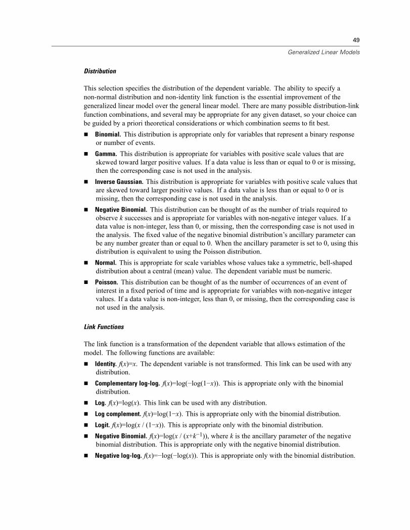
49

Generalized Linear Models

Distribution

This selection specifies the distribution of the dependent variable. The ability to specify anon-normal distribution and non-identity link function is the essential improvement of thegeneralized linear model over the general linear model. There are many possible distribution-linkfunction combinations, and several may be appropriate for any given dataset, so your choice canbe guided by a priori theoretical considerations or which combination seems to fit best.

Binomial. This distribution is appropriate only for variables that represent a binary responseor number of events.Gamma. This distribution is appropriate for variables with positive scale values that areskewed toward larger positive values. If a data value is less than or equal to 0 or is missing,then the corresponding case is not used in the analysis.Inverse Gaussian. This distribution is appropriate for variables with positive scale values thatare skewed toward larger positive values. If a data value is less than or equal to 0 or ismissing, then the corresponding case is not used in the analysis.Negative Binomial. This distribution can be thought of as the number of trials required toobserve k successes and is appropriate for variables with non-negative integer values. If adata value is non-integer, less than 0, or missing, then the corresponding case is not used inthe analysis. The fixed value of the negative binomial distribution’s ancillary parameter canbe any number greater than or equal to 0. When the ancillary parameter is set to 0, using thisdistribution is equivalent to using the Poisson distribution.Normal. This is appropriate for scale variables whose values take a symmetric, bell-shapeddistribution about a central (mean) value. The dependent variable must be numeric.Poisson. This distribution can be thought of as the number of occurrences of an event ofinterest in a fixed period of time and is appropriate for variables with non-negative integervalues. If a data value is non-integer, less than 0, or missing, then the corresponding case isnot used in the analysis.

Link Functions

The link function is a transformation of the dependent variable that allows estimation of themodel. The following functions are available:

Identity. f(x)=x. The dependent variable is not transformed. This link can be used with anydistribution.Complementary log-log. f(x)=log(−log(1−x)). This is appropriate only with the binomialdistribution.Log. f(x)=log(x). This link can be used with any distribution.Log complement. f(x)=log(1−x). This is appropriate only with the binomial distribution.Logit. f(x)=log(x / (1−x)). This is appropriate only with the binomial distribution.Negative Binomial. f(x)=log(x / (x+k−1)), where k is the ancillary parameter of the negativebinomial distribution. This is appropriate only with the negative binomial distribution.Negative log-log. f(x)=−log(−log(x)). This is appropriate only with the binomial distribution.

50

Chapter 6

Odds power. f(x)=[(x/(1−x))α−1]/α, if α ≠ 0. f(x)=log(x), if α=0. α is the required numberspecification and must be a real number. This is appropriate only with the binomialdistribution.Probit. f(x)=Φ−1(x), where Φ−1 is the inverse standard normal cumulative distributionfunction. This is appropriate only with the binomial distribution.Power. f(x)=xα, if α ≠ 0. f(x)=log(x), if α=0. α is the required number specification and mustbe a real number. This link can be used with any distribution.

Scale Weight. The scale parameter is an estimated model parameter related to the variance of theresponse. The scale weights are “known” values that can vary from observation to observation.If the scale weight variable is specified, the scale parameter, which is related to the variance ofthe response, is divided by it for each observation. Cases with scale weight values that are lessthan or equal to 0 or are missing are not used in the analysis.

Generalized Linear Models Reference CategoryFigure 6-2Generalized Linear Models Reference Category dialog box

For binary response, you can choose the reference category for the dependent variable. This canaffect certain output, such as parameter estimates and saved values, but it should not change themodel fit. For example, if your binary response takes values 0 and 1:

By default, the procedure makes the last (highest-valued) category, or 1, the referencecategory. In this situation, model-saved probabilities estimate the chance that a given casetakes the value 0, and parameter estimates should be interpreted as relating to the likelihoodof category 0.If you specify the first (lowest-valued) category, or 0, as the reference category, thenmodel-saved probabilities estimate the chance that a given case takes the value 1.If you specify the custom category and your variable has defined labels, you can set thereference category by choosing a value from the list. This can be convenient when, in themiddle of specifying a model, you don’t remember exactly how a particular variable wascoded.

51


Generalized Linear Models PredictorsFigure 6-3Generalized Linear Models: Predictors tab

The Predictors tab allows you to specify the factors and covariates used to build model effects andto specify an optional offset.

Factors. Factors are categorical predictors; they can be numeric or string. You can specify optionsto be universally applied to the factors.

Covariates. Covariates are scale predictors; they must be numeric.

Note: When the response is binomial with binary format, the procedure computes deviance andchi-square goodness-of-fit statistics by subpopulations that are based on the cross-classification ofobserved values of the selected factors and covariates. You should keep the same set of predictorsacross multiple runs of the procedure to ensure a consistent number of subpopulations.

Offset. The offset term is a “structural” predictor. Its coefficient is not estimated by the modelbut is assumed to have the value 1; thus, the values of the offset are simply added to the linearpredictor of the dependent variable. This is especially useful in Poisson regression models, whereeach case may have different levels of exposure to the event of interest. For example, whenmodeling accident rates for individual drivers, there is an important difference between a driverwho has been at fault in 1 accident in 3 years of experience and a driver who has been at fault in

52

Chapter 6

1 accident in 25 years! The number of accidents can be modeled as a Poisson response if theexperience of the driver is included as an offset term.

Generalized Linear Models OptionsFigure 6-4Generalized Linear Models Options dialog box

These options are applied to all factors specified on the Predictors tab.

User-Missing Values. Factors must have valid values for a case to be included in the analysis.These controls allow you to decide whether user-missing values are treated as valid amongfactor variables.

Category Order. This is relevant for determining a factor’s last level, which may be associated witha redundant parameter in the estimation algorithm. Changing the category order can change thevalues of factor-level effects, since these parameter estimates are calculated relative to the “last”level. Factors can be sorted in ascending order from lowest to highest value, in descending orderfrom highest to lowest value, or in “data order.” This means that the first value encountered in thedata defines the first category, and the last unique value encountered defines the last category.

53


Generalized Linear Models ModelFigure 6-5Generalized Linear Models: Model tab

Specify Model Effects. The default model is intercept-only, so you must explicitly specify othermodel effects. Alternatively, you can build nested or non-nested terms.

Non-Nested Terms



Interaction. Creates the highest-level interaction term for all selected variables.

Factorial. Creates all possible interactions and main effects of the selected variables.





54

Chapter 6

Nested Terms

You can build nested terms for your model in this procedure. Nested terms are useful formodeling the effect of a factor or covariate whose values do not interact with the levels of anotherfactor. For example, a grocery store chain may follow the spending habits of its customers atseveral store locations. Since each customer frequents only one of these locations, the Customereffect can be said to be nested within the Store location effect.Additionally, you can include interaction effects, such as polynomial terms involving the same

covariate, or add multiple levels of nesting to the nested term.


Generalized Linear Models EstimationFigure 6-6Generalized Linear Models: Estimation tab

55


Parameter Estimation. The controls in this group allow you to specify estimation methods and toprovide initial values for the parameter estimates.

Method. You can select a parameter estimation method. Choose between Newton-Raphson,Fisher scoring, or a hybrid method in which Fisher scoring iterations are performed beforeswitching to the Newton-Raphson method. If convergence is achieved during the Fisherscoring phase of the hybrid method before the maximum number of Fisher iterations isreached, the algorithm continues with the Newton-Raphson method.Scale parameter method. You can select the scale parameter estimation method.Maximum-likelihood jointly estimates the scale parameter with the model effects; notethat this option is not valid if the response has a negative binomial, poisson, or binomialdistribution. The deviance and Pearson chi-square options estimate the scale parameterfrom the value of those statistics. Alternatively, you can specify a fixed value for the scaleparameter.Initial values. The procedure will automatically compute initial values for parameters.Alternatively, you can specify initial values for the parameter estimates.Covariance matrix. The model-based estimator is the negative of the generalized inverse of theHessian matrix. The robust (also called the Huber/White/sandwich) estimator is a “corrected”model-based estimator that provides a consistent estimate of the covariance, even when thespecification of the variance and link functions is incorrect.

Iterations.

Maximum iterations. The maximum number of iterations the algorithm will execute. Specify anon-negative integer.Maximum step-halving. At each iteration, the step size is reduced by a factor of 0.5 until thelog-likelihood increases or maximum step-halving is reached. Specify a positive integer.Check for separation. When selected, the algorithm performs tests to ensure that the parameterestimates have unique values. Separation occurs when the procedure can produce a modelthat correctly classifies every case. This option is available for binomial responses withbinary format.

Convergence Criteria.

Parameter convergence. When selected, the algorithm stops after an iteration in which theabsolute or relative change in the parameter estimates is less than the value specified, whichmust be positive.Log-likelihood convergence. When selected, the algorithm stops after an iteration in whichthe absolute or relative change in the log-likelihood function is less than the value specified,which must be positive.Hessian convergence. For the Absolute specification, convergence is assumed if a statisticbased on the Hessian convergence is less than the positive value specified. For the Relativespecification, convergence is assumed if the statistic is less than the product of the positivevalue specified and the absolute value of the log-likelihood.

56

Chapter 6

Singularity Tolerance. Singular (or non-invertible) matrices have linearly dependent columns,which can cause serious problems for the estimation algorithm. Even near-singular matricescan lead to poor results, so the procedure will treat a matrix whose determinant is less than thetolerance as singular. Specify a positive value.

Generalized Linear Models Initial ValuesFigure 6-7Generalized Linear Models Initial Values dialog box

If initial values are specified, they must be supplied for all parameters (including redundantparameters) in the model. In the SPSS dataset, the ordering of variables from left to right must be:RowType_, VarName_, P1, P2, …, where RowType_ and VarName_ are string variables and P1,P2, … are numeric variables corresponding to an ordered list of the parameters.

Initial values are supplied on a record with value EST for variable RowType_; the actual initialvalues are given under variables P1, P2, …. The procedure ignores all records for whichRowType_ has a value other than EST as well as any records beyond the first occurrence ofRowType_ equal to EST.The intercept, if included in the model, must be the first initial value, P1.The maximum-likelihood estimate of the scale parameter, if that method is used, must be thelast initial value specified.If Split File is in effect, then the variables must begin with the split-file variable or variables inthe order specified when creating the Split File, followed by RowType_, VarName_, P1, P2, …as above. Splits must occur in the specified dataset in the same order as in the original dataset.

Note: The variable names P1, P2, … are not required; the procedure will accept any valid variablenames for the parameters because the mapping of variables to parameters is based on variableposition, not variable name. Any variables beyond the last parameter are ignored.

The file structure for the initial values is the same as that used when exporting the model as data;thus, you can use the final values from one run of the procedure as input in a subsequent run.

57


Generalized Linear Models StatisticsFigure 6-8Generalized Linear Models: Statistics tab

Model Effects.

Analysis Type. Specify the type of analysis to produce. Type I analysis is generally appropriatewhen you have a priori reasons for ordering predictors in the model, while Type III is moregenerally applicable. Wald statistics are produced in any case.Confidence intervals. Specify a confidence level greater than 50 and less than 100. Waldintervals are based on the assumption that parameters have an asymptotic normal distribution.Log-likelihood function. This controls the display format of the log-likelihood function. Thefull function includes an additional term that is constant with respect to the parameterestimates; it has no effect on parameter estimation and is left out of the display in somesoftware products.

Print. The following output is available.Case processing summary. Displays the number and percentage of cases included andexcluded from the analysis.Descriptive statistics. Displays descriptive statistics and summary information about thedependent variable, covariates, and factors.

58

Chapter 6

Model information. Displays the dataset name, dependent variable or events and trialsvariables, offset variable, scale weight variable, probability distribution, and link function.Goodness of fit statistics. Displays deviance and scaled deviance, Pearson chi-square andscaled Pearson chi-square, log likelihood, Akaike’s information criterion (AIC), finite samplecorrected AIC (AICC), Bayesian information criterion (BIC), consistent AIC (CAIC).Model summary statistics. Displays model fit tests, including likelihood ratio statistics for themodel fit omnibus test and statistics for the Type I or Type III contrasts for each effect.Parameter estimates. Displays parameter estimates and corresponding test statistics andconfidence intervals. You can optionally display exponentiated parameter estimates inaddition to the raw parameter estimates.Covariance matrix for parameter estimates. Displays the estimated parameter covariancematrix.Correlation matrix for parameter estimates. Displays the estimated parameter correlationmatrix.Contrast coefficient (L) matrices. Displays contrast coefficients for the default effects and forthe estimated marginal means if requested on the EM Means tab.General estimable functions. Displays the matrices for generating the contrast coefficient (L)matrices.Iteration history. Displays the iteration history for the parameter estimates and log-likelihood,and prints the last evaluation of the gradient vector and the Hessian matrix. The iterationhistory table displays parameter estimates for every n iterations beginning with the 0thiteration (the initial estimates), where n is the value of the print interval. If the iterationhistory is requested, then the last iteration is always displayed regardless of n.Lagrange multiplier test. Displays Lagrange multiplier test statistics for assessing the validityof a scale parameter that is computed using the deviance or Pearson chi-square, or set at afixed number, for the normal, gamma, and inverse Gaussian distributions. For the negativebinomial distribution, this tests the fixed ancillary parameter.

59


Generalized Linear Models EM MeansFigure 6-9Generalized Linear Models: EM Means tab

This tab allows you to display the estimated marginal means for levels of factors and factorinteractions. You can also request that the overall estimated mean be displayed.

Factors and Interactions. This list contains factors specified on the Predictors tab and factorinteractions specified on the Model tab. Covariates are excluded from this list. Terms can beselected directly from this list or combined into an interaction term using the By * button.

Display Means For. Estimated means are computed for the selected factors and factor interactions.The contrast determines how hypothesis tests are set up to compare the estimated means. Thesimple contrast requires a reference category or factor level against which the others are compared.

Pairwise. Pairwise comparisons are computed for all-level combinations of the specified orimplied factors. This is the only available contrast for factor interactions.Simple. Compares the mean of each level to the mean of a specified level. This type ofcontrast is useful when there is a control group.Deviation. Each level of the factor is compared to the grand mean. Deviation contrasts arenot orthogonal.

60

Chapter 6

Difference. Compares the mean of each level (except the first) to the mean of previous levels.They are sometimes called reverse Helmert contrasts.Helmert. Compares the mean of each level of the factor (except the last) to the mean ofsubsequent levels.Repeated. Compares the mean of each level (except the last) to the mean of the subsequentlevel.Polynomial. Compares the linear effect, quadratic effect, cubic effect, and so on. Thefirst degree of freedom contains the linear effect across all categories; the second degreeof freedom, the quadratic effect; and so on. These contrasts are often used to estimatepolynomial trends.

Scale. Estimated marginal means can be computed for the response, based on the originalscale of the dependent variable, or for the linear predictor, based on the dependent variable astransformed by the link function.

Adjustment for Multiple Comparisons. When performing hypothesis tests with multiple contrasts,the overall significance level can be adjusted from the significance levels for the includedcontrasts. This group allows you to choose the adjustment method.

Least significant difference. This method does not control the overall probability of rejectingthe hypotheses that some linear contrasts are different from the null hypothesis values.Bonferroni. This method adjusts the observed significance level for the fact that multiplecontrasts are being tested.Sequential Bonferroni. This is a sequentially step-down rejective Bonferroni procedure that ismuch less conservative in terms of rejecting individual hypotheses but maintains the sameoverall significance level.Sidak. This method provides tighter bounds than the Bonferroni approach.Sequential Sidak. This is a sequentially step-down rejective Sidak procedure that is much lessconservative in terms of rejecting individual hypotheses but maintains the same overallsignificance level.

61


Generalized Linear Models SaveFigure 6-10Generalized Linear Models: Save tab

Checked items are saved with the specified name; you can choose to overwrite existing variableswith the same name as the new variables or avoid name conflicts by appendix suffixes to makethe new variable names unique.

Predicted value of mean of response. Saves model-predicted values for each case in theoriginal response metric.Confidence interval for mean of response. Saves the upper and lower bounds of the confidenceinterval for the mean of the response.Predicted value of linear predictor. Saves model-predicted values for each case in the metric ofthe linear predictor (transformed response via the specified link function).Estimated standard error of predicted value of linear predictor.

Cook’s distance. A measure of how much the residuals of all cases would change if a particularcase were excluded from the calculation of the regression coefficients. A large Cook’s Dindicates that excluding a case from computation of the regression statistics changes thecoefficients substantially.Leverage value. Measures the influence of a point on the fit of the regression. The centeredleverage ranges from 0 (no influence on the fit) to (N-1)/N.

62

Chapter 6

Raw residual. The difference between an observed value and the value predicted by the model.Pearson residual. The square root of the contribution of a case to the Pearson chi-squarestatistic, with the sign of the raw residual.Standardized Pearson residual. The Pearson residual multiplied by the square root of theinverse of the product of the scale parameter and 1−leverage for the case.Deviance residual. The square root of the contribution of a case to the Deviance statistic,with the sign of the raw residual.Standardized deviance residual. The Deviance residual multiplied by the square root of theinverse of the product of the scale parameter and 1−leverage for the case.Likelihood residual. The square root of a weighted average (based on the leverage of the case)of the squares of the standardized Pearson and standardized Deviance residuals, with thesign of the raw residual.

Generalized Linear Models ExportFigure 6-11Generalized Linear Models: Export tab

63


Export model as data. Writes an SPSS dataset containing the parameter correlation or covariancematrix with parameter estimates, standard errors, significance values, and degrees of freedom.You can use this matrix file as the initial values for further model estimation in this procedure orfor further analyses in other procedures that read an SPSS matrix file.

Export model as XML. Saves the parameter estimates and the parameter covariance matrix, ifselected, in XML (PMML) format. SmartScore and the server version of SPSS (a separateproduct) can use this model file to apply the model information to other data files for scoringpurposes.

GENLIN Command Additional Features

The SPSS command language also allows you to:Specify initial values for parameter estimates as a list of numbers (using the CRITERIAsubcommand).Fix covariates at values other than their means when computing estimated marginal means(using the EMMEANS subcommand).Specify custom polynomial contrasts for estimated marginal means (using the EMMEANSsubcommand).Specify a subset of the factors for which estimated marginal means are displayed to becompared using the specified contrast type (using the TABLES and COMPARE keywords of theEMMEANS subcommand).


Chapter

7Generalized Estimating Equations

The Generalized Estimating Equations procedure extends the generalized linear model to allowfor analysis of repeated measurements or other correlated observations, such as clustered data.

Data. The response can be scale, counts, binary, or events-in-trials. Factors are assumed to becategorical. The covariates, scale weight, and offset are assumed to be scale. Variables used todefine subjects or within-subject repeated measurements cannot be used to define the response butcan serve other roles in the model.

Assumptions. Cases are assumed to be dependent within subjects and independent betweensubjects. The correlation matrix that represents the within-subject dependencies is estimatedas part of the model.

Obtaining Generalized Estimating Equations


Generalized Linear ModelsGeneralized Estimating Equations...

64

65

Generalized Estimating Equations

Figure 7-1Generalized Estimating Equations: Repeated tab

E Select one or more subject variables (see below for further options).

The combination of values of the specified variables should uniquely define subjects withinthe dataset. For example, a single Patient ID variable should be sufficient to define subjectsin a single hospital, but the combination of Hospital ID and Patient ID may be necessary ifpatient identification numbers are not unique across hospitals. In a repeated measures setting,multiple observations are recorded for each subject, so each subject may occupy multiple cases inthe dataset.

E On the Response tab, select a dependent variable.

E On the Predictors tab, select factors and covariates for use in predicting the dependent variable.

E On the Model tab, specify model effects using the selected factors and covariates.

Optionally, on the Repeated tab you can specify:

Within-subject variables. The combination of values of the within-subject variables defines theordering of measurements within subjects; thus, the combination of within-subject and subjectvariables uniquely defines each measurement. For example, the combination of Period, Hospital

66

Chapter 7

ID, and Patient ID defines, for each case, a particular office visit for a particular patient withina particular hospital.If the dataset is already sorted so that each subject’s repeated measurements occur in a

contiguous block of cases and in the proper order, it is not strictly necessary to specify awithin-subjects variable, and you can deselect Sort cases by subject and within-subject variables

and save the processing time required to perform the (temporary) sort. Generally, it’s a good ideato make use of within-subject variables to ensure proper ordering of measurements.

Subject and within-subject variables cannot be used to define the response, but they can performother functions in the model. For example, Hospital ID could be used as a factor in the model.

Covariance Matrix. The model-based estimator is the negative of the generalized inverse of theHessian matrix. The robust estimator (also called the Huber/White/sandwich estimator) is a“corrected” model-based estimator that provides a consistent estimate of the covariance, evenwhen the working correlation matrix is misspecified. This specification applies to the parametersin the linear model part of the generalized estimating equations, while the specification on theEstimation tab applies only to the initial generalized linear model.

Working Correlation Matrix. This correlation matrix represents the within-subject dependencies.Its size is determined by the number of measurements and thus the combination of values ofwithin-subject variables. You can specify one of the following structures:

Independent. Repeated measurements are uncorrelated.AR(1). Repeated measurements have a first-order autoregressive relationship. The correlationbetween any two elements is equal to ρ for adjacent elements, ρ2 for elements that areseparated by a third, and so on. ρ is constrained so that –1<ρ<1.Exchangeable. This structure has homogenous correlations between elements. It is alsoknown as a compound symmetry structure.M-dependent. Consecutive measurements have a common correlation coefficient, pairs ofmeasurements separated by a third have a common correlation coefficient, and so on, throughpairs of measurements separated by m−1 other measurements. Measurements with greaterseparation are assumed to be uncorrelated. When choosing this structure, specify a valueof m less than the order of the working correlation matrix.Unstructured. This is a completely general correlation matrix.

By default, the procedure will adjust the correlation estimates by the number of nonredundantparameters. Removing this adjustment may be desirable if you want the estimates to be invariantto subject-level replication changes in the data.

Maximum iterations. The maximum number of iterations the generalized estimating equationsalgorithm will execute. Specify a non-negative integer. This specification applies to theparameters in the linear model part of the generalized estimating equations, while thespecification on the Estimation tab applies only to the initial generalized linear model.Update matrix. Elements in the working correlation matrix are estimated based on theparameter estimates, which are updated in each iteration of the algorithm. If the workingcorrelation matrix is not updated at all, the initial working correlation matrix is usedthroughout the estimation process. If the matrix is updated, you can specify the iteration

67


interval at which to update working correlation matrix elements. Specifying a value greaterthan 1 may reduce processing time.

Convergence criteria. These specifications apply to the parameters in the linear model part of thegeneralized estimating equations, while the specification on the Estimation tab applies only tothe initial generalized linear model.

Parameter convergence. When selected, the algorithm stops after an iteration in which theabsolute or relative change in the parameter estimates is less than the value specified, whichmust be positive.Hessian convergence. Convergence is assumed if a statistic based on the Hessian is less thanthe value specified, which must be positive.

Generalized Estimating Equations ResponseFigure 7-2Generalized Estimating Equations: Response tab

In many cases, you can simply specify a dependent variable; however, variables that take onlytwo values and responses that record events in trials require extra attention.

68

Chapter 7

Binary response.When the dependent variable takes only two values, you can specify thereference category for parameter estimation. A binary response variable can be string ornumeric.Number of events occurring in a set of trials. When the response is a number of eventsoccurring in a set of trials, the dependent variable contains the number of events and you canselect an additional variable containing the number of trials. Alternatively, if the number oftrials is the same across all subjects, then trials may be specified using a fixed value. Thenumber of trials should be greater than or equal to the number of events for each case. Eventsshould be non-negative integers, and trials should be positive integers.

Distribution

This selection specifies the distribution of the dependent variable. The ability to specify anon-normal distribution and non-identity link function is the essential improvement of thegeneralized linear model over the general linear model. There are many possible distribution-linkfunction combinations, and several may be appropriate for any given dataset, so your choice canbe guided by a priori theoretical considerations or which combination seems to fit best.

Binomial. This distribution is appropriate only for variables that represent a binary responseor number of events.Gamma. This distribution is appropriate for variables with positive scale values that areskewed toward larger positive values. If a data value is less than or equal to 0 or is missing,then the corresponding case is not used in the analysis.Inverse Gaussian. This distribution is appropriate for variables with positive scale values thatare skewed toward larger positive values. If a data value is less than or equal to 0 or ismissing, then the corresponding case is not used in the analysis.Negative Binomial. This distribution can be thought of as the number of trials required toobserve k successes and is appropriate for variables with non-negative integer values. If adata value is non-integer, less than 0, or missing, then the corresponding case is not used inthe analysis. The fixed value of the negative binomial distribution’s ancillary parameter canbe any number greater than or equal to 0. When the ancillary parameter is set to 0, using thisdistribution is equivalent to using the Poisson distribution.Normal. This is appropriate for scale variables whose values take a symmetric, bell-shapeddistribution about a central (mean) value. The dependent variable must be numeric.Poisson. This distribution can be thought of as the number of occurrences of an event ofinterest in a fixed period of time and is appropriate for variables with non-negative integervalues. If a data value is non-integer, less than 0, or missing, then the corresponding case isnot used in the analysis.

Link Function

The link function is a transformation of the dependent variable that allows estimation of themodel. The following functions are available:

Identity. f(x)=x. The dependent variable is not transformed. This link can be used with anydistribution.

69


Complementary log-log. f(x)=log(−log(1−x)). This is appropriate only with the binomialdistribution.Log. f(x)=log(x). This link can be used with any distribution.Log complement. f(x)=log(1−x). This is appropriate only with the binomial distribution.Logit. f(x)=log(x / (1−x)). This is appropriate only with the binomial distribution.Negative Binomial. f(x)=log(x / (x+k−1)), where k is the ancillary parameter of the negativebinomial distribution. This is appropriate only with the negative binomial distribution.Negative log-log. f(x)=−log(−log(x)). This is appropriate only with the binomial distribution.Odds power. f(x)=[(x/(1−x))α−1]/α, if α ≠ 0. f(x)=log(x), if α=0. α is the required numberspecification and must be a real number. This is appropriate only with the binomialdistribution.Probit. f(x)=Φ−1(x), where Φ−1 is the inverse standard normal cumulative distributionfunction. This is appropriate only with the binomial distribution.Power. f(x)=xα, if α ≠ 0. f(x)=log(x), if α=0. α is the required number specification and mustbe a real number. This link can be used with any distribution.

Scale Weight. The scale parameter is an estimated model parameter related to the variance of theresponse. The scale weights are “known” values that can vary from observation to observation.If the scale weight variable is specified, the scale parameter, which is related to the variance ofthe response, is divided by it for each observation. Cases with scale weight values that are lessthan or equal to 0 or are missing are not used in the analysis.

Generalized Estimating Equations Reference CategoryFigure 7-3Generalized Estimating Equations Reference Category dialog box

For binary response, you can choose the reference category for the dependent variable. This canaffect certain output, such as parameter estimates and saved values, but it should not change themodel fit. For example, if your binary response takes values 0 and 1:

By default, the procedure makes the last (highest-valued) category, or 1, the referencecategory. In this situation, model-saved probabilities estimate the chance that a given casetakes the value 0, and parameter estimates should be interpreted as relating to the likelihoodof category 0.

70

Chapter 7

If you specify the first (lowest-valued) category, or 0, as the reference category, thenmodel-saved probabilities estimate the chance that a given case takes the value 1.If you specify the custom category and your variable has defined labels, you can set thereference category by choosing a value from the list. This can be convenient when, in themiddle of specifying a model, you don’t remember exactly how a particular variable wascoded.

Generalized Estimating Equations PredictorsFigure 7-4Generalized Estimating Equations: Predictors tab

The Predictors tab allows you to specify the factors and covariates used to build model effects andto specify an optional offset.

Factors. Factors are categorical predictors; they can be numeric or string. You can specify optionsto be universally applied to the factors.

Covariates. Covariates are scale predictors; they must be numeric.

71


Note: When the response is binomial with binary format, the procedure computes deviance andchi-square goodness-of-fit statistics by subpopulations that are based on the cross-classification ofobserved values of the selected factors and covariates. You should keep the same set of predictorsacross multiple runs of the procedure to ensure a consistent number of subpopulations.

Offset. The offset term is a “structural” predictor. Its coefficient is not estimated by the modelbut is assumed to have the value 1; thus, the values of the offset are simply added to the linearpredictor of the dependent variable. This is especially useful in Poisson regression models, whereeach case may have different levels of exposure to the event of interest. For example, whenmodeling accident rates for individual drivers, there is an important difference between a driverwho has been at fault in 1 accident in 3 years of experience and a driver who has been at fault in1 accident in 25 years! The number of accidents can be modeled as a Poisson response if theexperience of the driver is included as an offset term.

Generalized Estimating Equations OptionsFigure 7-5Generalized Estimating Equations Options dialog box

These options are applied to all factors specified on the Predictors tab.

User-Missing Values. Factors must have valid values for a case to be included in the analysis.These controls allow you to decide whether user-missing values are treated as valid amongfactor variables.

Category Order. This is relevant for determining a factor’s last level, which may be associated witha redundant parameter in the estimation algorithm. Changing the category order can change thevalues of factor-level effects, since these parameter estimates are calculated relative to the “last”level. Factors can be sorted in ascending order from lowest to highest value, in descending orderfrom highest to lowest value, or in “data order.” This means that the first value encountered in thedata defines the first category, and the last unique value encountered defines the last category.

72

Chapter 7

Generalized Estimating Equations ModelFigure 7-6Generalized Estimating Equations: Model tab

Specify Model Effects. The default model is intercept-only, so you must explicitly specify othermodel effects. Alternatively, you can build nested or non-nested terms.

Non-Nested Terms



Interaction. Creates the highest-level interaction term for all selected variables.

Factorial. Creates all possible interactions and main effects of the selected variables.





73


Nested Terms

You can build nested terms for your model in this procedure. Nested terms are useful formodeling the effect of a factor or covariate whose values do not interact with the levels of anotherfactor. For example, a grocery store chain may follow the spending habits of its customers atseveral store locations. Since each customer frequents only one of these locations, the Customereffect can be said to be nested within the Store location effect.Additionally, you can include interaction effects or add multiple levels of nesting to the nested

term.


Generalized Estimating Equations EstimationFigure 7-7Generalized Estimating Equations: Estimation tab

74

Chapter 7

Parameter Estimation. The controls in this group allow you to specify estimation methods and toprovide initial values for the parameter estimates.

Method. You can select a parameter estimation method; choose between Newton-Raphson,Fisher scoring, or a hybrid method in which Fisher scoring iterations are performed beforeswitching to the Newton-Raphson method. If convergence is achieved during the Fisherscoring phase of the hybrid method before the maximum number of Fisher iterations isreached, the algorithm continues with the Newton-Raphson method.Scale Parameter Method. You can select the scale parameter estimation method.Maximum-likelihood jointly estimates the scale parameter with the model effects; notethat this option is not valid if the response has a negative binomial, Poisson, or binomialdistribution. Since the concept of likelihood does not enter into generalized estimatingequations, this specification applies only to the initial generalized linear model; this scaleparameter estimate is then passed to the generalized estimating equations, which update thescale parameter by the Pearson chi-square divided by its degrees of freedom.The deviance and Pearson chi-square options estimate the scale parameter from the value ofthose statistics in the initial generalized linear model; this scale parameter estimate is thenpassed to the generalized estimating equations, which treat it as fixed.Alternatively, specify a fixed value for the scale parameter. It will be treated as fixed inestimating the initial generalized linear model and the generalized estimating equations.Initial values. The procedure will automatically compute initial values for parameters.Alternatively, you can specify initial values for the parameter estimates.

The iterations and convergence criteria specified on this tab are applicable only to the initialgeneralized linear model. For estimation criteria used in fitting the generalized estimatingequations, see the Repeated tab.

Iterations.

Maximum iterations. The maximum number of iterations the algorithm will execute. Specify anon-negative integer.Maximum step-halving. At each iteration, the step size is reduced by a factor of 0.5 until thelog-likelihood increases or maximum step-halving is reached. Specify a positive integer.Check for separation. When selected, the algorithm performs tests to ensure that the parameterestimates have unique values. Separation occurs when the procedure can produce a modelthat correctly classifies every case. This option is available for binomial responses withbinary format.

Convergence Criteria.

Parameter convergence. When selected, the algorithm stops after an iteration in which theabsolute or relative change in the parameter estimates is less than the value specified, whichmust be positive.

75


Log-likelihood convergence. When selected, the algorithm stops after an iteration in whichthe absolute or relative change in the log-likelihood function is less than the value specified,which must be positive.Hessian convergence. For the Absolute specification, convergence is assumed if a statisticbased on the Hessian convergence is less than the positive value specified. For the Relativespecification, convergence is assumed if the statistic is less than the product of the positivevalue specified and the absolute value of the log-likelihood.

Singularity Tolerance. Singular (or non-invertible) matrices have linearly dependent columns,which can cause serious problems for the estimation algorithm. Even near-singular matricescan lead to poor results, so the procedure will treat a matrix whose determinant is less than thetolerance as singular. Specify a positive value.

Generalized Estimating Equations Initial Values

The procedure estimates an initial generalized linear model, and the estimates from this modelare used as initial values for the parameter estimates in the linear model part of the generalizedestimating equations. Initial values are not needed for the working correlation matrix becausematrix elements are based on the parameter estimates. Initial values specified on this dialogbox are used as the starting point for the initial generalized linear model, not the generalizedestimating equations, unless the Maximum iterations on the Estimation tab is set to 0.

Figure 7-8Generalized Estimating Equations Initial Values dialog box

If initial values are specified, they must be supplied for all parameters (including redundantparameters) in the model. In the SPSS dataset, the ordering of variables from left to right must be:RowType_, VarName_, P1, P2, …, where RowType_ and VarName_ are string variables and P1,P2, … are numeric variables corresponding to an ordered list of the parameters.

Initial values are supplied on a record with value EST for variable RowType_; the actual initialvalues are given under variables P1, P2, …. The procedure ignores all records for whichRowType_ has a value other than EST as well as any records beyond the first occurrence ofRowType_ equal to EST.The intercept, if included in the model, must be the first initial value, P1.

76

Chapter 7

The maximum-likelihood estimate of the scale parameter, if that method is used, must be thelast initial value specified.If Split File is in effect, then the variables must begin with the split-file variable or variables inthe order specified when creating the Split File, followed by RowType_, VarName_, P1, P2, …as above. Splits must occur in the specified dataset in the same order as in the original dataset.

Note: The variable names P1, P2, … are not required; the procedure will accept any valid variablenames for the parameters because the mapping of variables to parameters is based on variableposition, not variable name. Any variables beyond the last parameter are ignored.

The file structure for the initial values is the same as that used when exporting the model as data;thus, you can use the final values from one run of the procedure as input in a subsequent run.

Generalized Estimating Equations StatisticsFigure 7-9Generalized Estimating Equations: Statistics tab

Model Effects.

77


Analysis Type. Specify the type of analysis to produce. Type I analysis is generally appropriatewhen you have a priori reasons for ordering predictors in the model, while Type III is moregenerally applicable. Wald statistics are produced in any case.Confidence intervals. Specify a confidence level greater than 50 and less than 100. Waldintervals are based on the assumption that parameters have an asymptotic normal distribution.

Print. The following output is available:Case processing summary. Displays the number and percentage of cases included andexcluded from the analysis and the Correlated Data Summary table.Descriptive statistics. Displays descriptive statistics and summary information about thedependent variable, covariates, and factors.Model information. Displays the dataset name, dependent variable or events and trialsvariables, offset variable, scale weight variable, probability distribution, and link function.Goodness of fit statistics. Displays two extensions of Akaike’s Information Criterion for modelselection: Quasi-likelihood under the independence model criterion (QIC) for choosing thebest correlation structure and another QIC measure for choosing the best subset of predictors.Model summary statistics. Displays model fit tests, including likelihood-ratio statistics for themodel fit omnibus test and statistics for the type I or III contrasts for each effect.Parameter estimates. Displays parameter estimates and corresponding test statistics andconfidence intervals. You can optionally display exponentiated parameter estimates inaddition to the raw parameter estimates.Covariance matrix for parameter estimates. Displays the estimated parameter covariancematrix.Correlation matrix for parameter estimates. Displays the estimated parameter correlationmatrix.Contrast coefficient (L) matrices. Displays contrast coefficients for the default effects and forthe estimated marginal means, if requested on the EM Means tab.General estimable functions. Displays the matrices for generating the contrast coefficient (L)matrices.Iteration history. Displays the iteration history for the parameter estimates and log-likelihoodand prints the last evaluation of the gradient vector and the Hessian matrix. The iterationhistory table displays parameter estimates for every n iterations beginning with the 0thiteration (the initial estimates), where n is the value of the print interval. If the iterationhistory is requested, then the last iteration is always displayed regardless of n.

78

Chapter 7

Generalized Estimating Equations EM MeansFigure 7-10Generalized Estimating Equations: EM Means tab

This tab allows you to display the estimated marginal means for levels of factors and factorinteractions. You can also request that the overall estimated mean be displayed.

Factors and Interactions. This list contains factors specified on the Predictors tab and factorinteractions specified on the Model tab. Covariates are excluded from this list. Terms can beselected directly from this list or combined into an interaction term using the By * button.

Display Means For. Estimated means are computed for the selected factors and factor interactions.The contrast determines how hypothesis tests are set up to compare the estimated means. Thesimple contrast requires a reference category or factor level against which the others are compared.

Pairwise. Pairwise comparisons are computed for all-level combinations of the specified orimplied factors. This is the only available contrast for factor interactions.Simple. Compares the mean of each level to the mean of a specified level. This type ofcontrast is useful when there is a control group.Deviation. Each level of the factor is compared to the grand mean. Deviation contrasts arenot orthogonal.

79


Difference. Compares the mean of each level (except the first) to the mean of previous levels.They are sometimes called reverse Helmert contrasts.Helmert. Compares the mean of each level of the factor (except the last) to the mean ofsubsequent levels.Repeated. Compares the mean of each level (except the last) to the mean of the subsequentlevel.Polynomial. Compares the linear effect, quadratic effect, cubic effect, and so on. Thefirst degree of freedom contains the linear effect across all categories; the second degreeof freedom, the quadratic effect; and so on. These contrasts are often used to estimatepolynomial trends.

Scale. Estimated marginal means can be computed for the response, based on the originalscale of the dependent variable, or for the linear predictor, based on the dependent variable astransformed by the link function.

Adjustment for Multiple Comparisons. When performing hypothesis tests with multiple contrasts,the overall significance level can be adjusted from the significance levels for the includedcontrasts. This group allows you to choose the adjustment method.

Least significant difference. This method does not control the overall probability of rejectingthe hypotheses that some linear contrasts are different from the null hypothesis values.Bonferroni. This method adjusts the observed significance level for the fact that multiplecontrasts are being tested.Sequential Bonferroni. This is a sequentially step-down rejective Bonferroni procedure that ismuch less conservative in terms of rejecting individual hypotheses but maintains the sameoverall significance level.Sidak. This method provides tighter bounds than the Bonferroni approach.Sequential Sidak. This is a sequentially step-down rejective Sidak procedure that is much lessconservative in terms of rejecting individual hypotheses but maintains the same overallsignificance level.

80

Chapter 7

Generalized Estimating Equations SaveFigure 7-11Generalized Estimating Equations: Save tab

Checked items are saved with the specified name; you can choose to overwrite existing variableswith the same name as the new variables or avoid name conflicts by appendix suffixes to makethe new variable names unique.

Predicted value of mean of response. Saves model-predicted values for each case in theoriginal response metric.Confidence interval for mean of response. Saves the upper and lower bounds of the confidenceinterval for the mean of the response.Predicted value of linear predictor. Saves model-predicted values for each case in the metric ofthe linear predictor (transformed response via the specified link function).Estimated standard error of predicted value of linear predictor.

Raw residual. The difference between an observed value and the value predicted by the model.Pearson residual. The square root of the contribution of a case to the Pearson chi-squarestatistic, with the sign of the raw residual.

Note: Cook’s distances, leverage values, standardized Pearson residuals, deviance residuals,standardized deviances residuals, and likelihood residuals are never available.

81


Generalized Estimating Equations ExportFigure 7-12Generalized Estimating Equations: Export tab

Export model as data. Writes an SPSS dataset containing the parameter correlation or covariancematrix with parameter estimates, standard errors, significance values, and degrees of freedom.You can use this matrix file as the initial values for further model estimation in this procedure orfor further analyses in other procedures that read an SPSS matrix file.

Export model as XML. Saves the parameter estimates and the parameter covariance matrix, ifselected, in XML (PMML) format. SmartScore and the server version of SPSS (a separateproduct) can use this model file to apply the model information to other data files for scoringpurposes.

GENLIN Command Additional Features

The SPSS command language also allows you to:Specify initial values for parameter estimates as a list of numbers (using the CRITERIAsubcommand).Specify a fixed working correlation matrix (using the REPEATED subcommand).

82

Chapter 7

Fix covariates at values other than their means when computing estimated marginal means(using the EMMEANS subcommand).Specify custom polynomial contrasts for estimated marginal means (using the EMMEANSsubcommand).Specify a subset of the factors for which estimated marginal means are displayed to becompared using the specified contrast type (using the TABLES and COMPARE keywords of theEMMEANS subcommand).


Chapter

8Model Selection Loglinear Analysis

The Model Selection Loglinear Analysis procedure analyzes multiway crosstabulations(contingency tables). It fits hierarchical loglinear models to multidimensional crosstabulationsusing an iterative proportional-fitting algorithm. This procedure helps you find out whichcategorical variables are associated. To build models, forced entry and backward eliminationmethods are available. For saturated models, you can request parameter estimates and tests ofpartial association. A saturated model adds 0.5 to all cells.

Example. In a study of user preference for one of two laundry detergents, researchers countedpeople in each group, combining various categories of water softness (soft, medium, or hard),previous use of one of the brands, and washing temperature (cold or hot). They found howtemperature is related to water softness and also to brand preference.

Statistics. Frequencies, residuals, parameter estimates, standard errors, confidence intervals, andtests of partial association. For custom models, plots of residuals and normal probability plots.

Data. Factor variables are categorical. All variables to be analyzed must be numeric. Categoricalstring variables can be recoded to numeric variables before starting the model selection analysis.Avoid specifying many variables with many levels. Such specifications can lead to a situation

where many cells have small numbers of observations, and the chi-square values may notbe useful.

Related procedures. The Model Selection procedure can help identify the terms needed in themodel. Then you can continue to evaluate the model using General Loglinear Analysis or LogitLoglinear Analysis. You can use Autorecode to recode string variables. If a numeric variable hasempty categories, use Recode to create consecutive integer values.

Obtaining a Model Selection Loglinear Analysis


LoglinearModel Selection...

83

84

Chapter 8

Figure 8-1Model Selection Loglinear Analysis dialog box

E Select two or more numeric categorical factors.

E Select one or more factor variables in the Factor(s) list, and click Define Range.

E Define the range of values for each factor variable.

E Select an option in the Model Building group.

Optionally, you can select a cell weight variable to specify structural zeros.

Loglinear Analysis Define RangeFigure 8-2Loglinear Analysis Define Range dialog box

You must indicate the range of categories for each factor variable. Values for Minimum andMaximum correspond to the lowest and highest categories of the factor variable. Both valuesmust be integers, and the minimum value must be less than the maximum value. Cases withvalues outside of the bounds are excluded. For example, if you specify a minimum value of 1and a maximum value of 3, only the values 1, 2, and 3 are used. Repeat this process for eachfactor variable.

85

Model Selection Loglinear Analysis

Loglinear Analysis ModelFigure 8-3Loglinear Analysis Model dialog box

Specify Model. A saturated model contains all factor main effects and all factor-by-factorinteractions. Select Custom to specify a generating class for an unsaturated model.

Generating Class. A generating class is a list of the highest-order terms in which factors appear.SPSS builds a hierarchical model containing the terms that define the generating class and alllower-order relatives. Suppose you select variables A, B, and C in the Factors list and then selectInteraction from the Build Terms drop-down list. The resulting model will contain the specified3-way interaction A*B*C, the 2-way interactions A*B, A*C, and B*C, and main effects for A, B,and C. Do not specify the lower-order relatives in the generating class.

Build Terms








86

Chapter 8

Model Selection Loglinear Analysis OptionsFigure 8-4Loglinear Analysis Options dialog box

Display. You can choose Frequencies, Residuals, or both. In a saturated model, the observed andexpected frequencies are equal, and the residuals are equal to 0.

Display for Saturated Model. For a saturated model, you can choose Parameter estimates. Theparameter estimates may help determine which terms can be dropped from the model. Anassociation table, which lists tests of partial association, is also available. This option iscomputationally expensive for tables with many factors.

Plot. For custom models, you can choose one or both types of plots, Residuals and Normal

probability. These will help determine how well a model fits the data.

Model Criteria. SPSS uses an iterative proportional-fitting algorithm to obtain parameter estimates.You can override one or more of the estimation criteria by specifying Maximum iterations,Convergence, or Delta (a value added to all cell frequencies for saturated models).

HILOGLINEAR Command Additional Features

The SPSS command language also allows you to:Specify cell weights in matrix form (using the CWEIGHT subcommand).Generate analyses of several models with a single command (using the DESIGN subcommand).


Chapter

9General Loglinear Analysis

The General Loglinear Analysis procedure analyzes the frequency counts of observationsfalling into each cross-classification category in a crosstabulation or a contingency table. Eachcross-classification in the table constitutes a cell, and each categorical variable is called a factor.The dependent variable is the number of cases (frequency) in a cell of the crosstabulation, and theexplanatory variables are factors and covariates. This procedure estimates maximum likelihoodparameters of hierarchical and nonhierarchical loglinear models using the Newton-Raphsonmethod. Either a Poisson or a multinomial distribution can be analyzed.You can select up to 10 factors to define the cells of a table. A cell structure variable allows

you to define structural zeros for incomplete tables, include an offset term in the model, fit alog-rate model, or implement the method of adjustment of marginal tables. Contrast variablesallow computation of generalized log-odds ratios (GLOR).SPSS automatically displays model information and goodness-of-fit statistics. You can also

display a variety of statistics and plots or save residuals and predicted values in the active dataset.

Example. Data from a report of automobile accidents in Florida are used to determine therelationship between wearing a seat belt and whether an injury was fatal or nonfatal. The oddsratio indicates significant evidence of a relationship.

Statistics. Observed and expected frequencies; raw, adjusted, and deviance residuals; designmatrix; parameter estimates; odds ratio; log-odds ratio; GLOR; Wald statistic; and confidenceintervals. Plots: adjusted residuals, deviance residuals, and normal probability.

Data. Factors are categorical, and cell covariates are continuous. When a covariate is in themodel, SPSS applies the mean covariate value for cases in a cell to that cell. Contrast variablesare continuous. They are used to compute generalized log-odds ratios. The values of the contrastvariable are the coefficients for the linear combination of the logs of the expected cell counts.A cell structure variable assigns weights. For example, if some of the cells are structural zeros,

the cell structure variable has a value of either 0 or 1. Do not use a cell structure variable toweight aggregated data. Instead, choose Weight Cases from the Data menu.

Assumptions. Two distributions are available in General Loglinear Analysis: Poisson andmultinomial.

Under the Poisson distribution assumption:The total sample size is not fixed before the study, or the analysis is not conditional on thetotal sample size.The event of an observation being in a cell is statistically independent of the cell countsof other cells.

87

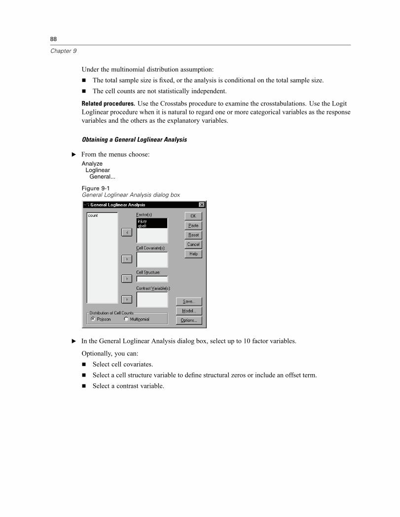
88

Chapter 9

Under the multinomial distribution assumption:The total sample size is fixed, or the analysis is conditional on the total sample size.The cell counts are not statistically independent.

Related procedures. Use the Crosstabs procedure to examine the crosstabulations. Use the LogitLoglinear procedure when it is natural to regard one or more categorical variables as the responsevariables and the others as the explanatory variables.

Obtaining a General Loglinear Analysis


LoglinearGeneral...

Figure 9-1General Loglinear Analysis dialog box

E In the General Loglinear Analysis dialog box, select up to 10 factor variables.

Optionally, you can:Select cell covariates.Select a cell structure variable to define structural zeros or include an offset term.Select a contrast variable.

89

General Loglinear Analysis

General Loglinear Analysis ModelFigure 9-2General Loglinear Analysis Model dialog box

Specify Model. A saturated model contains all main effects and interactions involving factorvariables. It does not contain covariate terms. Select Custom to specify only a subset ofinteractions or to specify factor-by-covariate interactions.

Factors and Covariates. The factors and covariates are listed, with (Cov) indicating a covariate.

Terms in Model. The model depends on the nature of your data. After selecting Custom, you canselect the main effects and interactions that are of interest in your analysis. You must indicateall of the terms to be included in the model.

Build Terms








90

Chapter 9

General Loglinear Analysis OptionsFigure 9-3General Loglinear Analysis Options dialog box

The General Loglinear Analysis procedure displays model information and goodness-of-fitstatistics. In addition, you can choose one or more of the following:

Display. Several statistics are available for display—observed and expected cell frequencies;raw, adjusted, and deviance residuals; a design matrix of the model; and parameter estimatesfor the model.

Plot. Plots, available for custom models only, include two scatterplot matrices (adjusted residualsor deviance residuals against observed and expected cell counts). You can also display normalprobability and detrended normal plots of adjusted residuals or deviance residuals.

Confidence Interval. The confidence interval for parameter estimates can be adjusted.

Criteria. The Newton-Raphson method is used to obtain maximum likelihood parameterestimates. You can enter new values for the maximum number of iterations, the convergencecriterion, and delta (a constant added to all cells for initial approximations). Delta remains in thecells for saturated models.

General Loglinear Analysis SaveFigure 9-4General Loglinear Analysis Save dialog box

91

General Loglinear Analysis

Select the values you want to save as new variables in the active dataset. The suffix n in the newvariable names increments to make a unique name for each saved variable.The saved values refer to the aggregated data (cells in the contingency table), even if the data

are recorded in individual observations in the Data Editor. If you save residuals or predictedvalues for unaggregated data, the saved value for a cell in the contingency table is entered in theData Editor for each case in that cell. To make sense of the saved values, you should aggregatethe data to obtain the cell counts.Four types of residuals can be saved: raw, standardized, adjusted, and deviance. The predicted

values can also be saved.Residuals. Also called the simple or raw residual, it is the difference between the observedcell count and its expected count.Standardized residuals. The residual divided by an estimate of its standard error. Standardizedresiduals are also known as Pearson residuals.Adjusted residuals. The standardized residual divided by its estimated standard error. Sincethe adjusted residuals are asymptotically standard normal when the selected model is correct,they are preferred over the standardized residuals for checking for normality.Deviance residuals. The signed square root of an individual contribution to the likelihood-ratiochi-square statistic (G squared), where the sign is the sign of the residual (observed countminus expected count). Deviance residuals have an asymptotic standard normal distribution.

GENLOG Command Additional FeaturesThe SPSS command language also allows you to:

Calculate linear combinations of observed cell frequencies and expected cell frequencies, andprint residuals, standardized residuals, and adjusted residuals of that combination (using theGERESID subcommand).Change the default threshold value for redundancy checking (using the CRITERIAsubcommand).Display the standardized residuals (using the PRINT subcommand).


Chapter

10Logit Loglinear Analysis

The Logit Loglinear Analysis procedure analyzes the relationship between dependent (orresponse) variables and independent (or explanatory) variables. The dependent variablesare always categorical, while the independent variables can be categorical (factors). Otherindependent variables, cell covariates, can be continuous, but they are not applied on acase-by-case basis. The weighted covariate mean for a cell is applied to that cell. The logarithmof the odds of the dependent variables is expressed as a linear combination of parameters.A multinomial distribution is automatically assumed; these models are sometimes calledmultinomial logit models. This procedure estimates parameters of logit loglinear models usingthe Newton-Raphson algorithm.You can select from 1 to 10 dependent and factor variables combined. A cell structure variable

allows you to define structural zeros for incomplete tables, include an offset term in the model, fita log-rate model, or implement the method of adjustment of marginal tables. Contrast variablesallow computation of generalized log-odds ratios (GLOR). The values of the contrast variable arethe coefficients for the linear combination of the logs of the expected cell counts.SPSS automatically displays model information and goodness-of-fit statistics. You can also

display a variety of statistics and plots or save residuals and predicted values in the active dataset.

Example. A study in Florida included 219 alligators. How does the alligators’ food type varywith their size and the four lakes in which they live? The study found that the odds of a smalleralligator preferring reptiles to fish is 0.70 times lower than for larger alligators; also, the odds ofselecting primarily reptiles instead of fish were highest in lake 3.

Statistics. Observed and expected frequencies; raw, adjusted, and deviance residuals; designmatrix; parameter estimates; generalized log-odds ratio; Wald statistic; and confidence intervals.Plots: adjusted residuals, deviance residuals, and normal probability plots.

Data. The dependent variables are categorical. Factors are categorical. Cell covariates can becontinuous, but when a covariate is in the model, SPSS applies the mean covariate value for casesin a cell to that cell. Contrast variables are continuous. They are used to compute generalizedlog-odds ratios (GLOR). The values of the contrast variable are the coefficients for the linearcombination of the logs of the expected cell counts.A cell structure variable assigns weights. For example, if some of the cells are structural zeros,

the cell structure variable has a value of either 0 or 1. Do not use a cell structure variable toweight aggregate data. Instead, use Weight Cases on the Data menu.

Assumptions. The counts within each combination of categories of explanatory variables areassumed to have a multinomial distribution. Under the multinomial distribution assumption:

The total sample size is fixed, or the analysis is conditional on the total sample size.The cell counts are not statistically independent.

92

93

Logit Loglinear Analysis

Related procedures. Use the Crosstabs procedure to display the contingency tables. Use theGeneral Loglinear Analysis procedure when you want to analyze the relationship between anobserved count and a set of explanatory variables.

Obtaining a Logit Loglinear Analysis


LoglinearLogit...

Figure 10-1Logit Loglinear Analysis dialog box

E In the Logit Loglinear Analysis dialog box, select one or more dependent variables.

E Select one or more factor variables.

The total number of dependent and factor variables must be less than or equal to 10.

Optionally, you can:Select cell covariates.Select a cell structure variable to define structural zeros or include an offset term.Select one or more contrast variables.

94

Chapter 10

Logit Loglinear Analysis ModelFigure 10-2Logit Loglinear Analysis Model dialog box

Specify Model. A saturated model contains all main effects and interactions involving factorvariables. It does not contain covariate terms. Select Custom to specify only a subset ofinteractions or to specify factor-by-covariate interactions.

Factors and Covariates. The factors and covariates are listed, with (Cov) indicating a covariate.

Terms in Model. The model depends on the nature of your data. After selecting Custom, you canselect the main effects and interactions that are of interest in your analysis. You must indicateall of the terms to be included in the model.Terms are added to the design by taking all possible combinations of the dependent terms and

matching each combination with each term in the model list. If Include constant for dependent isselected, there is also a unit term (1) added to the model list.For example, suppose variables D1 and D2 are the dependent variables. A dependent terms list

is created by the Logit Loglinear Analysis procedure (D1, D2, D1*D2). If the Terms in Modellist contains M1 and M2 and a constant is included, the model list contains 1, M1, and M2. Theresultant design includes combinations of each model term with each dependent term:

D1, D2, D1*D2

M1*D1, M1*D2, M1*D1*D2

M2*D1, M2*D2, M2*D1*D2

Include constant for dependent. Includes a constant for the dependent variable in a custom model.

Build Terms




95

Logit Loglinear Analysis





Logit Loglinear Analysis OptionsFigure 10-3Logit Loglinear Analysis Options dialog box

The Logit Loglinear Analysis procedure displays model information and goodness-of-fit statistics.In addition, you can choose one or more of the following options:

Display. Several statistics are available for display: observed and expected cell frequencies;raw, adjusted, and deviance residuals; a design matrix of the model; and parameter estimatesfor the model.

Plot. Plots available for custom models include two scatterplot matrices (adjusted residuals ordeviance residuals against observed and expected cell counts). You can also display normalprobability and detrended normal plots of adjusted residuals or deviance residuals.

Confidence Interval. The confidence interval for parameter estimates can be adjusted.

Criteria. The Newton-Raphson method is used to obtain maximum likelihood parameterestimates. You can enter new values for the maximum number of iterations, the convergencecriterion, and delta (a constant added to all cells for initial approximations). Delta remains in thecells for saturated models.

96

Chapter 10

Logit Loglinear Analysis SaveFigure 10-4Logit Loglinear Analysis Save dialog box

Select the values you want to save as new variables in the active dataset. The suffix n in the newvariable names increments to make a unique name for each saved variable.The saved values refer to the aggregated data (to cells in the contingency table), even if the

data are recorded in individual observations in the Data Editor. If you save residuals or predictedvalues for unaggregated data, the saved value for a cell in the contingency table is entered in theData Editor for each case in that cell. To make sense of the saved values, you should aggregatethe data to obtain the cell counts.Four types of residuals can be saved: raw, standardized, adjusted, and deviance. The predicted

values can also be saved.Residuals. Also called the simple or raw residual, it is the difference between the observedcell count and its expected count.Standardized residuals. The residual divided by an estimate of its standard error. Standardizedresiduals are also known as Pearson residuals.Adjusted residuals. The standardized residual divided by its estimated standard error. Sincethe adjusted residuals are asymptotically standard normal when the selected model is correct,they are preferred over the standardized residuals for checking for normality.Deviance residuals. The signed square root of an individual contribution to the likelihood-ratiochi-square statistic (G squared), where the sign is the sign of the residual (observed countminus expected count). Deviance residuals have an asymptotic standard normal distribution.

GENLOG Command Additional Features

The SPSS command language also allows you to:Calculate linear combinations of observed cell frequencies and expected cell frequencies, andprint residuals, standardized residuals, and adjusted residuals of that combination (using theGERESID subcommand).Change the default threshold value for redundancy checking (using the CRITERIAsubcommand).Display the standardized residuals (using the PRINT subcommand).


Chapter

11Life Tables

There are many situations in which you would want to examine the distribution of times betweentwo events, such as length of employment (time between being hired and leaving the company).However, this kind of data usually includes some cases for which the second event isn’t recorded(for example, people still working for the company at the end of the study). This can happen forseveral reasons: for some cases, the event simply doesn’t occur before the end of the study; forother cases, we lose track of their status sometime before the end of the study; still other casesmay be unable to continue for reasons unrelated to the study (such as an employee becoming illand taking a leave of absence). Collectively, such cases are known as censored cases, and theymake this kind of study inappropriate for traditional techniques such as t tests or linear regression.A statistical technique useful for this type of data is called a follow-up life table. The basic

idea of the life table is to subdivide the period of observation into smaller time intervals. For eachinterval, all people who have been observed at least that long are used to calculate the probabilityof a terminal event occurring in that interval. The probabilities estimated from each of the intervalsare then used to estimate the overall probability of the event occurring at different time points.

Example. Is a new nicotine patch therapy better than traditional patch therapy in helping people toquit smoking? You could conduct a study using two groups of smokers, one of which receivedthe traditional therapy and the other of which received the experimental therapy. Constructinglife tables from the data would allow you to compare overall abstinence rates between thetwo groups to determine if the experimental treatment is an improvement over the traditionaltherapy. You can also plot the survival or hazard functions and compare them visually for moredetailed information.

Statistics. Number entering, number leaving, number exposed to risk, number of terminal events,proportion terminating, proportion surviving, cumulative proportion surviving (and standarderror), probability density (and standard error), and hazard rate (and standard error) for each timeinterval for each group; median survival time for each group; and Wilcoxon (Gehan) test forcomparing survival distributions between groups. Plots: function plots for survival, log survival,density, hazard rate, and one minus survival.

Data. Your time variable should be quantitative. Your status variable should be dichotomous orcategorical, coded as integers, with events being coded as a single value or a range of consecutivevalues. Factor variables should be categorical, coded as integers.

Assumptions. Probabilities for the event of interest should depend only on time after the initialevent—they are assumed to be stable with respect to absolute time. That is, cases that enterthe study at different times (for example, patients who begin treatment at different times)should behave similarly. There should also be no systematic differences between censored anduncensored cases. If, for example, many of the censored cases are patients with more seriousconditions, your results may be biased.

97

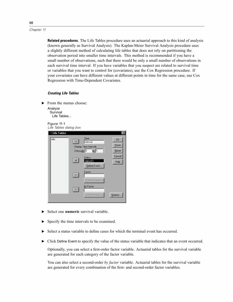
98

Chapter 11

Related procedures. The Life Tables procedure uses an actuarial approach to this kind of analysis(known generally as Survival Analysis). The Kaplan-Meier Survival Analysis procedure usesa slightly different method of calculating life tables that does not rely on partitioning theobservation period into smaller time intervals. This method is recommended if you have asmall number of observations, such that there would be only a small number of observations ineach survival time interval. If you have variables that you suspect are related to survival timeor variables that you want to control for (covariates), use the Cox Regression procedure. Ifyour covariates can have different values at different points in time for the same case, use CoxRegression with Time-Dependent Covariates.

Creating Life Tables


SurvivalLife Tables...

Figure 11-1Life Tables dialog box

E Select one numeric survival variable.

E Specify the time intervals to be examined.

E Select a status variable to define cases for which the terminal event has occurred.

E Click Define Event to specify the value of the status variable that indicates that an event occurred.

Optionally, you can select a first-order factor variable. Actuarial tables for the survival variableare generated for each category of the factor variable.

You can also select a second-order by factor variable. Actuarial tables for the survival variableare generated for every combination of the first- and second-order factor variables.

99

Life Tables

Life Tables Define Events for Status VariablesFigure 11-2Life Tables Define Event for Status Variable dialog box

Occurrences of the selected value or values for the status variable indicate that the terminal eventhas occurred for those cases. All other cases are considered to be censored. Enter either a singlevalue or a range of values that identifies the event of interest.

Life Tables Define RangeFigure 11-3Life Tables Define Range dialog box

Cases with values for the factor variable in the range you specify will be included in the analysis,and separate tables (and plots, if requested) will be generated for each unique value in the range.

Life Tables OptionsFigure 11-4Life Tables Options dialog box

You can control various aspects of your Life Tables analysis.

Life tables. To suppress the display of life tables in the output, deselect Life tables.

100

Chapter 11

Plot. Allows you to request plots of the survival functions. If you have defined factor variable(s),plots are generated for each subgroup defined by the factor variable(s). Available plots aresurvival, log survival, hazard, density, and one minus survival.

Survival. Displays the cumulative survival function on a linear scale.Log survival. Displays the cumulative survival function on a logarithmic scale.Hazard. Displays the cumulative hazard function on a linear scale.Density. Displays the density function.One minus survival. Plots one-minus the survival function on a linear scale.

Compare Levels of First Factor. If you have a first-order control variable, you can select one of thealternatives in this group to perform the Wilcoxon (Gehan) test, which compares the survivalof subgroups. Tests are performed on the first-order factor. If you have defined a second-orderfactor, tests are performed for each level of the second-order variable.

SURVIVAL Command Additional Features

The SPSS command language also allows you to:Specify more than one dependent variable.Specify unequally spaced intervals.Specify more than one status variable.Specify comparisons that do not include all the factor and all the control variables.Calculate approximate, rather than exact, comparisons.


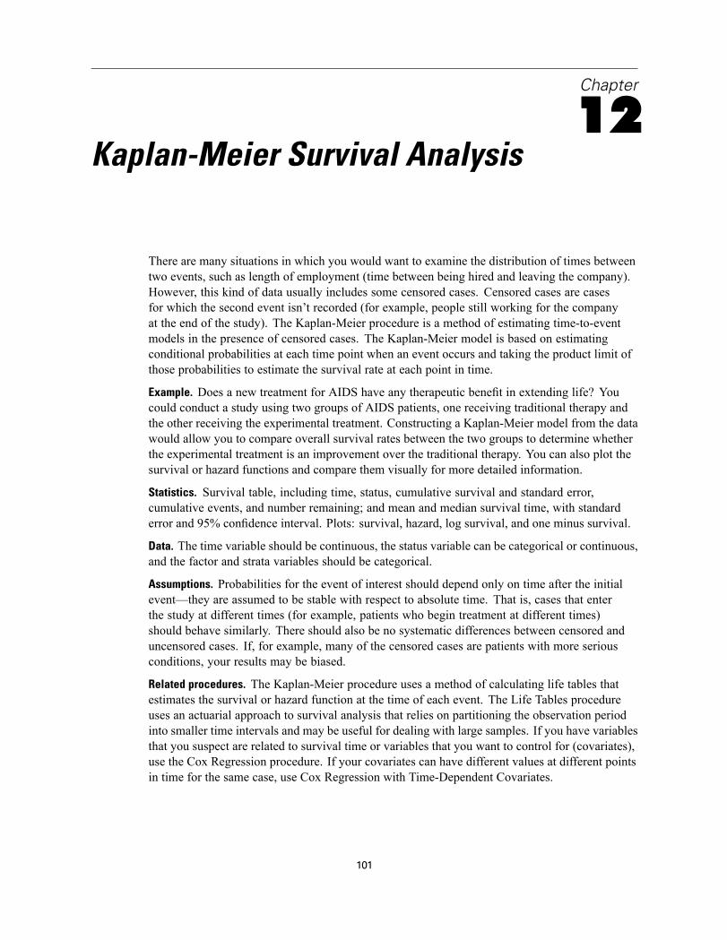
Chapter

12Kaplan-Meier Survival Analysis

There are many situations in which you would want to examine the distribution of times betweentwo events, such as length of employment (time between being hired and leaving the company).However, this kind of data usually includes some censored cases. Censored cases are casesfor which the second event isn’t recorded (for example, people still working for the companyat the end of the study). The Kaplan-Meier procedure is a method of estimating time-to-eventmodels in the presence of censored cases. The Kaplan-Meier model is based on estimatingconditional probabilities at each time point when an event occurs and taking the product limit ofthose probabilities to estimate the survival rate at each point in time.

Example. Does a new treatment for AIDS have any therapeutic benefit in extending life? Youcould conduct a study using two groups of AIDS patients, one receiving traditional therapy andthe other receiving the experimental treatment. Constructing a Kaplan-Meier model from the datawould allow you to compare overall survival rates between the two groups to determine whetherthe experimental treatment is an improvement over the traditional therapy. You can also plot thesurvival or hazard functions and compare them visually for more detailed information.

Statistics. Survival table, including time, status, cumulative survival and standard error,cumulative events, and number remaining; and mean and median survival time, with standarderror and 95% confidence interval. Plots: survival, hazard, log survival, and one minus survival.

Data. The time variable should be continuous, the status variable can be categorical or continuous,and the factor and strata variables should be categorical.

Assumptions. Probabilities for the event of interest should depend only on time after the initialevent—they are assumed to be stable with respect to absolute time. That is, cases that enterthe study at different times (for example, patients who begin treatment at different times)should behave similarly. There should also be no systematic differences between censored anduncensored cases. If, for example, many of the censored cases are patients with more seriousconditions, your results may be biased.

Related procedures. The Kaplan-Meier procedure uses a method of calculating life tables thatestimates the survival or hazard function at the time of each event. The Life Tables procedureuses an actuarial approach to survival analysis that relies on partitioning the observation periodinto smaller time intervals and may be useful for dealing with large samples. If you have variablesthat you suspect are related to survival time or variables that you want to control for (covariates),use the Cox Regression procedure. If your covariates can have different values at different pointsin time for the same case, use Cox Regression with Time-Dependent Covariates.

101

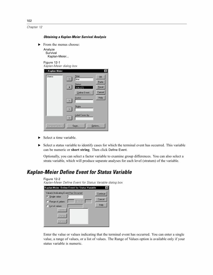
102

Chapter 12

Obtaining a Kaplan-Meier Survival Analysis


SurvivalKaplan-Meier...

Figure 12-1Kaplan-Meier dialog box

E Select a time variable.

E Select a status variable to identify cases for which the terminal event has occurred. This variablecan be numeric or short string. Then click Define Event.

Optionally, you can select a factor variable to examine group differences. You can also select astrata variable, which will produce separate analyses for each level (stratum) of the variable.

Kaplan-Meier Define Event for Status VariableFigure 12-2Kaplan-Meier Define Event for Status Variable dialog box

Enter the value or values indicating that the terminal event has occurred. You can enter a singlevalue, a range of values, or a list of values. The Range of Values option is available only if yourstatus variable is numeric.

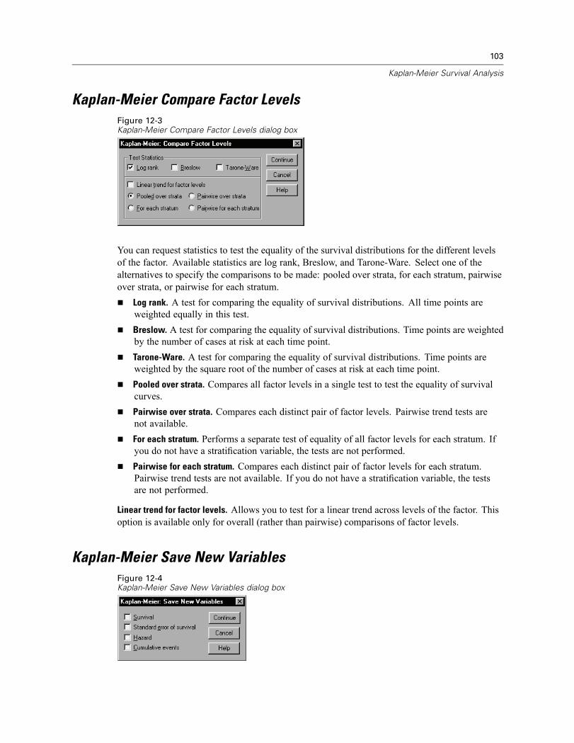
103

Kaplan-Meier Survival Analysis

Kaplan-Meier Compare Factor LevelsFigure 12-3Kaplan-Meier Compare Factor Levels dialog box

You can request statistics to test the equality of the survival distributions for the different levelsof the factor. Available statistics are log rank, Breslow, and Tarone-Ware. Select one of thealternatives to specify the comparisons to be made: pooled over strata, for each stratum, pairwiseover strata, or pairwise for each stratum.

Log rank. A test for comparing the equality of survival distributions. All time points areweighted equally in this test.Breslow. A test for comparing the equality of survival distributions. Time points are weightedby the number of cases at risk at each time point.Tarone-Ware. A test for comparing the equality of survival distributions. Time points areweighted by the square root of the number of cases at risk at each time point.Pooled over strata. Compares all factor levels in a single test to test the equality of survivalcurves.Pairwise over strata. Compares each distinct pair of factor levels. Pairwise trend tests arenot available.For each stratum. Performs a separate test of equality of all factor levels for each stratum. Ifyou do not have a stratification variable, the tests are not performed.Pairwise for each stratum. Compares each distinct pair of factor levels for each stratum.Pairwise trend tests are not available. If you do not have a stratification variable, the testsare not performed.

Linear trend for factor levels. Allows you to test for a linear trend across levels of the factor. Thisoption is available only for overall (rather than pairwise) comparisons of factor levels.

Kaplan-Meier Save New VariablesFigure 12-4Kaplan-Meier Save New Variables dialog box

104

Chapter 12

You can save information from your Kaplan-Meier table as new variables, which can then be usedin subsequent analyses to test hypotheses or check assumptions. You can save survival, standarderror of survival, hazard, and cumulative events as new variables.

Survival. Cumulative survival probability estimate. The default variable name is the prefixsur_ with a sequential number appended to it. For example, if sur_1 already exists,Kaplan-Meier assigns the variable name sur_2.Standard error of survival. Standard error of the cumulative survival estimate. The defaultvariable name is the prefix se_ with a sequential number appended to it. For example, if se_1already exists, Kaplan-Meier assigns the variable name se_2.Hazard. Cumulative hazard function estimate. The default variable name is the prefix haz_with a sequential number appended to it. For example, if haz_1 already exists, Kaplan-Meierassigns the variable name haz_2.Cumulative events. Cumulative frequency of events when cases are sorted by their survivaltimes and status codes. The default variable name is the prefix cum_ with a sequentialnumber appended to it. For example, if cum_1 already exists, Kaplan-Meier assigns thevariable name cum_2.

Kaplan-Meier OptionsFigure 12-5Kaplan-Meier Options dialog box

You can request various output types from Kaplan-Meier analysis.

Statistics. You can select statistics displayed for the survival functions computed, includingsurvival table(s), mean and median survival, and quartiles. If you have included factor variables,separate statistics are generated for each group.

Plots. Plots allow you to examine the survival, one-minus-survival, hazard, and log-survivalfunctions visually. If you have included factor variables, functions are plotted for each group.

Survival. Displays the cumulative survival function on a linear scale.One minus survival. Plots one-minus the survival function on a linear scale.Hazard. Displays the cumulative hazard function on a linear scale.Log survival. Displays the cumulative survival function on a logarithmic scale.

105

Kaplan-Meier Survival Analysis

KM Command Additional Features

The SPSS command language also allows you to:Obtain frequency tables that consider cases lost to follow-up as a separate category fromcensored cases.Specify unequal spacing for the test for linear trend.Obtain percentiles other than quartiles for the survival time variable.


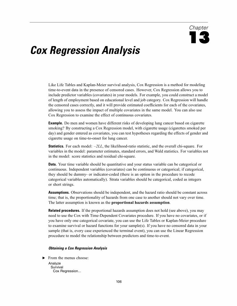
Chapter

13Cox Regression Analysis

Like Life Tables and Kaplan-Meier survival analysis, Cox Regression is a method for modelingtime-to-event data in the presence of censored cases. However, Cox Regression allows you toinclude predictor variables (covariates) in your models. For example, you could construct a modelof length of employment based on educational level and job category. Cox Regression will handlethe censored cases correctly, and it will provide estimated coefficients for each of the covariates,allowing you to assess the impact of multiple covariates in the same model. You can also useCox Regression to examine the effect of continuous covariates.

Example. Do men and women have different risks of developing lung cancer based on cigarettesmoking? By constructing a Cox Regression model, with cigarette usage (cigarettes smoked perday) and gender entered as covariates, you can test hypotheses regarding the effects of gender andcigarette usage on time-to-onset for lung cancer.

Statistics. For each model: –2LL, the likelihood-ratio statistic, and the overall chi-square. Forvariables in the model: parameter estimates, standard errors, and Wald statistics. For variables notin the model: score statistics and residual chi-square.

Data. Your time variable should be quantitative and your status variable can be categorical orcontinuous. Independent variables (covariates) can be continuous or categorical; if categorical,they should be dummy- or indicator-coded (there is an option in the procedure to recodecategorical variables automatically). Strata variables should be categorical, coded as integersor short strings.

Assumptions. Observations should be independent, and the hazard ratio should be constant acrosstime; that is, the proportionality of hazards from one case to another should not vary over time.The latter assumption is known as the proportional hazards assumption.

Related procedures. If the proportional hazards assumption does not hold (see above), you mayneed to use the Cox with Time-Dependent Covariates procedure. If you have no covariates, or ifyou have only one categorical covariate, you can use the Life Tables or Kaplan-Meier procedureto examine survival or hazard functions for your sample(s). If you have no censored data in yoursample (that is, every case experienced the terminal event), you can use the Linear Regressionprocedure to model the relationship between predictors and time-to-event.

Obtaining a Cox Regression Analysis


SurvivalCox Regression...

106

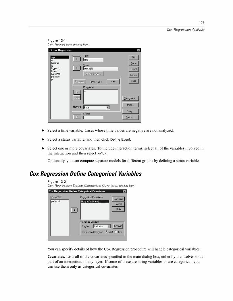
107

Cox Regression Analysis

Figure 13-1Cox Regression dialog box

E Select a time variable. Cases whose time values are negative are not analyzed.

E Select a status variable, and then click Define Event.

E Select one or more covariates. To include interaction terms, select all of the variables involved inthe interaction and then select >a*b>.

Optionally, you can compute separate models for different groups by defining a strata variable.

Cox Regression Define Categorical VariablesFigure 13-2Cox Regression Define Categorical Covariates dialog box

You can specify details of how the Cox Regression procedure will handle categorical variables.

Covariates. Lists all of the covariates specified in the main dialog box, either by themselves or aspart of an interaction, in any layer. If some of these are string variables or are categorical, youcan use them only as categorical covariates.

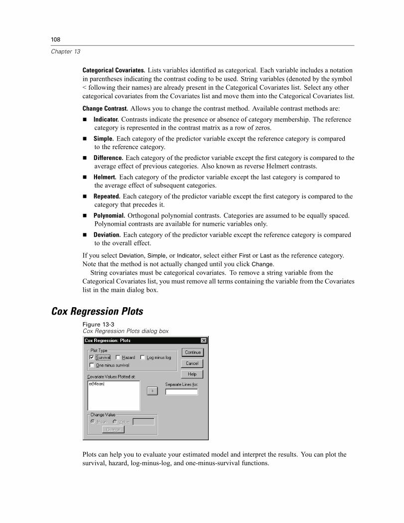
108

Chapter 13

Categorical Covariates. Lists variables identified as categorical. Each variable includes a notationin parentheses indicating the contrast coding to be used. String variables (denoted by the symbol< following their names) are already present in the Categorical Covariates list. Select any othercategorical covariates from the Covariates list and move them into the Categorical Covariates list.

Change Contrast. Allows you to change the contrast method. Available contrast methods are:Indicator. Contrasts indicate the presence or absence of category membership. The referencecategory is represented in the contrast matrix as a row of zeros.Simple. Each category of the predictor variable except the reference category is comparedto the reference category.Difference. Each category of the predictor variable except the first category is compared to theaverage effect of previous categories. Also known as reverse Helmert contrasts.Helmert. Each category of the predictor variable except the last category is compared tothe average effect of subsequent categories.Repeated. Each category of the predictor variable except the first category is compared to thecategory that precedes it.Polynomial. Orthogonal polynomial contrasts. Categories are assumed to be equally spaced.Polynomial contrasts are available for numeric variables only.Deviation. Each category of the predictor variable except the reference category is comparedto the overall effect.

If you select Deviation, Simple, or Indicator, select either First or Last as the reference category.Note that the method is not actually changed until you click Change.String covariates must be categorical covariates. To remove a string variable from the

Categorical Covariates list, you must remove all terms containing the variable from the Covariateslist in the main dialog box.

Cox Regression PlotsFigure 13-3Cox Regression Plots dialog box

Plots can help you to evaluate your estimated model and interpret the results. You can plot thesurvival, hazard, log-minus-log, and one-minus-survival functions.

109


Survival. Displays the cumulative survival function on a linear scale.Hazard. Displays the cumulative hazard function on a linear scale.Log minus log. The cumulative survival estimate after the ln(-ln) transformation is appliedto the estimate.One minus survival. Plots one-minus the survival function on a linear scale.

Because these functions depend on values of the covariates, you must use constant values forthe covariates to plot the functions versus time. The default is to use the mean of each covariateas a constant value, but you can enter your own values for the plot using the Change Valuecontrol group.You can plot a separate line for each value of a categorical covariate by moving that covariate

into the Separate Lines For text box. This option is available only for categorical covariates,which are denoted by (Cat) after their names in the Covariate Values Plotted At list.

Cox Regression Save New VariablesFigure 13-4Cox Regression Save New Variables dialog box

You can save various results of your analysis as new variables. These variables can then be usedin subsequent analyses to test hypotheses or to check assumptions.

Survival. Allows you to save the survival function, standard error, and log-minus-log estimates asnew variables.

Diagnostics. Allows you to save the hazard function, partial residuals, and DfBeta(s) for theregression as new variables.

Hazard function. Saves the cumulative hazard function estimate (also called the Cox-Snellresidual).Partial residuals. You can plot partial residuals against survival time to test the proportionalhazards assumption. One variable is saved for each covariate in the final model. Paritalresiduals are available only for models containing at least one covariate.DfBetas. Estimated change in a coefficient if a case is removed. One variable is saved foreach covariate in the final model. DfBetas are only available for models containing at leastone covariate.

If you are running Cox with a time-dependent covariate, DfBeta(s) are the only variables that youcan save. You can also save the linear predictor variable X*Beta.

X*Beta. Linear predictor score. The sum of the product of mean-centered covariate valuesand their corresponding parameter estimates for each case.

110

Chapter 13

Cox Regression OptionsFigure 13-5Cox Regression Options dialog box

You can control various aspects of your analysis and output.

Model Statistics. You can obtain statistics for your model parameters, including confidenceintervals for exp(B) and correlation of estimates. You can request these statistics either at eachstep or at the last step only.

Probability for Stepwise. If you have selected a stepwise method, you can specify the probabilityfor either entry or removal from the model. A variable is entered if the significance level of itsF-to-enter is less than the Entry value, and a variable is removed if the significance level is greaterthan the Removal value. The Entry value must be less than the Removal value.

Maximum Iterations. Allows you to specify the maximum iterations for the model, which controlshow long the procedure will search for a solution.

Display baseline function. Allows you to display the baseline hazard function and cumulativesurvival at the mean of the covariates. This display is not available if you have specifiedtime-dependent covariates.

Cox Regression Define Event for Status Variable

Enter the value or values indicating that the terminal event has occurred. You can enter a singlevalue, a range of values, or a list of values. The Range of Values option is available only if yourstatus variable is numeric.

COXREG Command Additional Features

The SPSS command language also allows you to:Obtain frequency tables that consider cases lost to follow-up as a separate category fromcensored cases.Select a reference category, other than first or last, for the deviation, simple, and indicatorcontrast methods.Specify unequal spacing of categories for the polynomial contrast method.Specify additional iteration criteria.Control the treatment of missing values.

111


Specify the names for saved variables.Write output to an external SPSS system file.Hold data for each split-file group in an external scratch file during processing. This can helpconserve memory resources when running analyses with large data sets. This is not availablewith time-dependent covariates.


Chapter

14Computing Time-DependentCovariates

There are certain situations in which you would want to compute a Cox Regression model but theproportional hazards assumption does not hold. That is, hazard ratios change across time; thevalues of one (or more) of your covariates are different at different time points. In such cases, youneed to use an extended Cox Regression model, which allows you to specify time-dependentcovariates.In order to analyze such a model, you must first define your time-dependent covariate.

(Multiple time-dependent covariates can be specified using command syntax.) To facilitate this,a system variable representing time is available. This variable is called T_. You can use thisvariable to define time-dependent covariates in two general ways:

If you want to test the proportional hazards assumption with respect to a particular covariateor estimate an extended Cox regression model that allows nonproportional hazards, you cando so by defining your time-dependent covariate as a function of the time variable T_ andthe covariate in question. A common example would be the simple product of the timevariable and the covariate, but more complex functions can be specified as well. Testing thesignificance of the coefficient of the time-dependent covariate will tell you whether theproportional hazards assumption is reasonable.Some variables may have different values at different time periods but aren’t systematicallyrelated to time. In such cases, you need to define a segmented time-dependent covariate,which can be done using logical expressions. Logical expressions take the value 1 if trueand 0 if false. Using a series of logical expressions, you can create your time-dependentcovariate from a set of measurements. For example, if you have blood pressure measuredonce a week for the four weeks of your study (identified as BP1 to BP4), you can define yourtime-dependent covariate as (T_ < 1) * BP1 + (T_ >= 1 & T_ < 2) * BP2 + (T_ >= 2 & T_ <3) * BP3 + (T_ >= 3 & T_ < 4) * BP4. Notice that exactly one of the terms in parentheseswill be equal to 1 for any given case and the rest will all equal 0. In other words, this functionmeans that if time is less than one week, use BP1; if it is more than one week but less thantwo weeks, use BP2, and so on.

For segmented time-dependent covariates, cases that are missing any values are removed fromthe analysis. Therefore, you must be sure that all cases have values for all measured time pointson the covariate, even for time points after the case is removed from the risk set (due to eventor censoring). These values are not used in the analysis, but they must be valid SPSS values toprevent the cases from being dropped. For example, with the definition given above, a casecensored at the second week must still have values for BP3 and BP4 (they can be 0 or any othernumber, since they are not used in the analysis).

112

113

Computing Time-Dependent Covariates

In the Compute Time-Dependent Covariate dialog box, you can use the function-buildingcontrols to build the expression for the time-dependent covariate, or you can enter it directly inthe Expression for T_COV_ text area. Note that string constants must be enclosed in quotationmarks or apostrophes, and numeric constants must be typed in American format, with the dotas the decimal delimiter. The resulting variable is called T_COV_ and should be included asa covariate in your Cox Regression model.

Computing a Time-Dependent CovariateE From the menus choose:

AnalyzeSurvival

Cox w/ Time-Dep Cov...

Figure 14-1Compute Time-Dependent Covariate dialog box

E Enter an expression for the time-dependent covariate.

E Click Model to proceed with your Cox Regression.

Note: Be sure to include the new variable T_COV_ as a covariate in your Cox Regression model.

For more information, see Cox Regression Analysis in Chapter 13 on p. 106.

Cox Regression with Time-Dependent Covariates Additional Features

The SPSS command language also allows you to specify multiple time-dependent covariates.Other command syntax features are available for Cox Regression with or without time-dependentcovariates.


Appendix

ACategorical Variable Coding Schemes

In many SPSS procedures, you can request automatic replacement of a categorical independentvariable with a set of contrast variables, which will then be entered or removed from an equationas a block. You can specify how the set of contrast variables is to be coded, usually on theCONTRAST subcommand. This appendix explains and illustrates how different contrast typesrequested on CONTRAST actually work.

Deviation

Deviation from the grand mean. In matrix terms, these contrasts have the form:

mean ( 1/k 1/k ... 1/k 1/k )df(1) ( 1–1/k –1/k ... –1/k –1/k )df(2) ( –1/k 1–1/k ... –1/k –1/k )

. .

. .

df(k–1) ( –1/k –1/k ... 1–1/k –1/k )

where k is the number of categories for the independent variable and the last category is omittedby default. For example, the deviation contrasts for an independent variable with three categoriesare as follows:

( 1/3 1/3 1/3 )( 2/3 –1/3 –1/3 )( –1/3 2/3 –1/3 )

To omit a category other than the last, specify the number of the omitted category in parenthesesafter the DEVIATION keyword. For example, the following subcommand obtains the deviationsfor the first and third categories and omits the second:

/CONTRAST(FACTOR)=DEVIATION(2)

Suppose that factor has three categories. The resulting contrast matrix will be

( 1/3 1/3 1/3 )( 2/3 –1/3 –1/3 )( –1/3 –1/3 2/3 )

114

115

Categorical Variable Coding Schemes

Simple

Simple contrasts. Compares each level of a factor to the last. The general matrix form is

mean ( 1/k 1/k ... 1/k 1/k )df(1) ( 1 0 ... 0 –1 )df(2) ( 0 1 ... 0 –1 )

. .

. .

df(k–1) ( 0 0 ... 1 –1 )

where k is the number of categories for the independent variable. For example, the simplecontrasts for an independent variable with four categories are as follows:

( 1/4 1/4 1/4 1/4 )( 1 0 0 –1 )( 0 1 0 –1 )( 0 0 1 –1 )

To use another category instead of the last as a reference category, specify in parentheses after theSIMPLE keyword the sequence number of the reference category, which is not necessarily thevalue associated with that category. For example, the following CONTRAST subcommand obtainsa contrast matrix that omits the second category:

/CONTRAST(FACTOR) = SIMPLE(2)

Suppose that factor has four categories. The resulting contrast matrix will be

( 1/4 1/4 1/4 1/4 )( 1 –1 0 0 )( 0 –1 1 0 )( 0 –1 0 1 )

Helmert

Helmert contrasts. Compares categories of an independent variable with the mean of thesubsequent categories. The general matrix form is

mean ( 1/k 1/k ... 1/k 1/k )df(1) ( 1 –1/(k–1) ... –1/(k–1) –1/(k–1) )df(2) ( 0 1 ... –1/(k–2) –1/(k–2) )

. .

. .

116

Appendix A

df(k–2) ( 0 0 1 –1/2 –1/2df(k–1) ( 0 0 ... 1 –1 )

where k is the number of categories of the independent variable. For example, an independentvariable with four categories has a Helmert contrast matrix of the following form:

( 1/4 1/4 1/4 1/4 )( 1 –1/3 –1/3 –1/3 )( 0 1 –1/2 –1/2 )( 0 0 1 –1 )

Difference

Difference or reverse Helmert contrasts. Compares categories of an independent variable with themean of the previous categories of the variable. The general matrix form is

mean ( 1/k 1/k 1/k ... 1/k )df(1) ( –1 1 0 ... 0 )df(2) ( –1/2 –1/2 1 ... 0 )

. .

. .

df(k–1) ( –1/(k–1) –1/(k–1) –1/(k–1) ... 1 )

where k is the number of categories for the independent variable. For example, the differencecontrasts for an independent variable with four categories are as follows:

( 1/4 1/4 1/4 1/4 )( –1 1 0 0 )( –1/2 –1/2 1 0 )( –1/3 –1/3 –1/3 1 )

Polynomial

Orthogonal polynomial contrasts. The first degree of freedom contains the linear effect across allcategories; the second degree of freedom, the quadratic effect; the third degree of freedom, thecubic; and so on, for the higher-order effects.You can specify the spacing between levels of the treatment measured by the given categorical

variable. Equal spacing, which is the default if you omit the metric, can be specified asconsecutive integers from 1 to k, where k is the number of categories. If the variable drug hasthree categories, the subcommand

/CONTRAST(DRUG)=POLYNOMIAL

is the same as

117


/CONTRAST(DRUG)=POLYNOMIAL(1,2,3)

Equal spacing is not always necessary, however. For example, suppose that drug representsdifferent dosages of a drug given to three groups. If the dosage administered to the second groupis twice that given to the first group and the dosage administered to the third group is three timesthat given to the first group, the treatment categories are equally spaced, and an appropriate metricfor this situation consists of consecutive integers:


If, however, the dosage administered to the second group is four times that given to the firstgroup, and the dosage administered to the third group is seven times that given to the first group,an appropriate metric is


In either case, the result of the contrast specification is that the first degree of freedom fordrug contains the linear effect of the dosage levels and the second degree of freedom containsthe quadratic effect.Polynomial contrasts are especially useful in tests of trends and for investigating the nature of

response surfaces. You can also use polynomial contrasts to perform nonlinear curve fitting, suchas curvilinear regression.

Repeated

Compares adjacent levels of an independent variable. The general matrix form is

mean ( 1/k 1/k 1/k ... 1/k 1/k )df(1) ( 1 –1 0 ... 0 0 )df(2) ( 0 1 –1 ... 0 0 )

. .

. .

df(k–1) ( 0 0 0 ... 1 –1 )

where k is the number of categories for the independent variable. For example, the repeatedcontrasts for an independent variable with four categories are as follows:

( 1/4 1/4 1/4 1/4 )( 1 –1 0 0 )( 0 1 –1 0 )( 0 0 1 –1 )

These contrasts are useful in profile analysis and wherever difference scores are needed.

118

Appendix A

Special

A user-defined contrast. Allows entry of special contrasts in the form of square matrices with asmany rows and columns as there are categories of the given independent variable. For MANOVAand LOGLINEAR, the first row entered is always the mean, or constant, effect and represents theset of weights indicating how to average other independent variables, if any, over the givenvariable. Generally, this contrast is a vector of ones.The remaining rows of the matrix contain the special contrasts indicating the desired

comparisons between categories of the variable. Usually, orthogonal contrasts are the mostuseful. Orthogonal contrasts are statistically independent and are nonredundant. Contrasts areorthogonal if:

For each row, contrast coefficients sum to 0.The products of corresponding coefficients for all pairs of disjoint rows also sum to 0.

For example, suppose that treatment has four levels and that you want to compare the variouslevels of treatment with each other. An appropriate special contrast is

( 1 1 1 1 ) weights for mean calculation( 3 –1 –1 –1 ) compare 1st with 2nd through 4th

( 0 2 –1 –1 ) compare 2nd with 3rd and 4th

( 0 0 1 –1 ) compare 3rd with 4th

which you specify by means of the following CONTRAST subcommand for MANOVA,LOGISTICREGRESSION, and COXREG:

/CONTRAST(TREATMNT)=SPECIAL( 1 1 1 13 -1 -1 -10 2 -1 -10 0 1 -1 )

For LOGLINEAR, you need to specify:

/CONTRAST(TREATMNT)=BASIS SPECIAL( 1 1 1 13 -1 -1 -10 2 -1 -10 0 1 -1 )

Each row except the means row sums to 0. Products of each pair of disjoint rows sum to 0 as well:

Rows 2 and 3: (3)(0) + (–1)(2) + (–1)(–1) + (–1)(–1) = 0Rows 2 and 4: (3)(0) + (–1)(0) + (–1)(1) + (–1)(–1) = 0Rows 3 and 4: (0)(0) + (2)(0) + (–1)(1) + (–1)(–1) = 0

The special contrasts need not be orthogonal. However, they must not be linear combinationsof each other. If they are, the procedure reports the linear dependency and ceases processing.Helmert, difference, and polynomial contrasts are all orthogonal contrasts.

119


Indicator

Indicator variable coding. Also known as dummy coding, this is not available in LOGLINEAR orMANOVA. The number of new variables coded is k–1. Cases in the reference category are coded 0for all k–1 variables. A case in the ith category is coded 0 for all indicator variables exceptthe ith, which is coded 1.

Appendix

BCovariance Structures

This section provides additional information on covariance structures.

Ante-Dependence: First-Order. This covariance structure has heterogenous variances andheterogenous correlations between adjacent elements. The correlation between two nonadjacentelements is the product of the correlations between the elements that lie between the elementsof interest.

AR(1). This is a first-order autoregressive structure with homogenous variances. The correlationbetween any two elements is equal to rho for adjacent elements, ρ2 for elements that are separatedby a third, and so on. ρ is constrained so that –1<ρ<1.

AR(1): Heterogenous. This is a first-order autoregressive structure with heterogenous variances.The correlation between any two elements is equal to ρ for adjacent elements, ρ2 for two elementsseparated by a third, and so on. ρ is constrained to lie between –1 and 1.

ARMA(1,1). This is a first-order autoregressive moving average structure. It has homogenousvariances. The correlation between two elements is equal to φ*ρ for adjacent elements, φ*(ρ2)for elements separated by a third, and so on. ρ and φ are the autoregressive and moving averageparameters, respectively, and their values are constrained to lie between –1 and 1, inclusive.

120

121

Covariance Structures

Compound Symmetry. This structure has constant variance and constant covariance.

Compound Symmetry: Correlation Metric. This covariance structure has homogenous variances andhomogenous correlations between elements.

Compound Symmetry: Heterogenous. This covariance structure has heterogenous variances andconstant correlation between elements.

Diagonal. This covariance structure has heterogenous variances and zero correlation betweenelements.

Factor Analytic: First-Order. This covariance structure has heterogenous variances that arecomposed of a term that is heterogenous across elements and a term that is homogenous acrosselements. The covariance between any two elements is the square root of the product of theirheterogenous variance terms.

122

Appendix B

Factor Analytic: First-Order, Heterogenous. This covariance structure has heterogenous variancesthat are composed of two terms that are heterogenous across elements. The covariance betweenany two elements is the square root of the product of the first of their heterogenous variance terms.

Huynh-Feldt. This is a “circular” matrix in which the covariance between any two elementsis equal to the average of their variances minus a constant. Neither the variances nor thecovariances are constant.

Scaled Identity. This structure has constant variance. There is assumed to be no correlationbetween any elements.

Toeplitz. This covariance structure has homogenous variances and heterogenous correlationsbetween elements. The correlation between adjacent elements is homogenous across pairs ofadjacent elements. The correlation between elements separated by a third is again homogenous,and so on.

Toeplitz: Heterogenous. This covariance structure has heterogenous variances and heterogenouscorrelations between elements. The correlation between adjacent elements is homogenousacross pairs of adjacent elements. The correlation between elements separated by a third isagain homogenous, and so on.

Unstructured. This is a completely general covariance matrix.

123

Covariance Structures

Unstructured: Correlation Metric. This covariance structure has heterogenous variances andheterogenous correlations.

Variance Components. This structure assigns a scaled identity (ID) structure to each of thespecified random effects.

Index

analysis of covariancein GLM Multivariate, 2

analysis of variancein Variance Components, 31

ANOVAin GLM Multivariate, 2in GLM Repeated Measures, 14

backward eliminationin Model Selection Loglinear Analysis, 83

Bartlett’s test of sphericityin GLM Multivariate, 11

Bonferroniin GLM Multivariate, 8in GLM Repeated Measures, 22

Box’s M testin GLM Multivariate, 11

Breslow testin Kaplan-Meier, 103

build terms, 5, 18, 30, 85, 89, 94

case processing summaryin Generalized Estimating Equations, 77in Generalized Linear Models, 57

censored casesin Cox Regression, 106in Kaplan-Meier, 101in Life Tables, 97

confidence intervalsin General Loglinear Analysis, 90in GLM Multivariate, 11in GLM Repeated Measures, 25in Linear Mixed Models, 43in Logit Loglinear Analysis, 95

contingency tablesin General Loglinear Analysis, 87

contrast coefficients matrixin Generalized Estimating Equations, 77in Generalized Linear Models, 58

contrastsin Cox Regression, 107in General Loglinear Analysis, 87in Logit Loglinear Analysis, 92

Cook’s distancein Generalized Linear Models, 61in GLM, 10in GLM Repeated Measures, 24

correlation matrixin Generalized Estimating Equations, 77in Generalized Linear Models, 58in Linear Mixed Models, 43

covariance matrixin Generalized Estimating Equations, 73, 77in Generalized Linear Models, 54, 58in GLM, 10in Linear Mixed Models, 43

covariance parameters testin Linear Mixed Models, 43

covariance structures, 120in Linear Mixed Models, 120

covariatesin Cox Regression, 107

Cox Regression, 106baseline functions, 110categorical covariates, 107command additional features, 110contrasts, 107covariates, 106define event, 110DfBeta(s), 109example, 106hazard function, 109iterations, 110partial residuals, 109plots, 108saving new variables, 109statistics, 106, 110stepwise entry and removal, 110string covariates, 107survival function, 109survival status variable, 110time-dependent covariates, 112–113

cross-productshypothesis and error matrices, 11

crosstabulationin Model Selection Loglinear Analysis, 83

custom modelsin GLM Repeated Measures, 18in Model Selection Loglinear Analysis, 85in Variance Components, 30

deleted residualsin GLM, 10in GLM Repeated Measures, 24

descriptive statisticsin Generalized Estimating Equations, 77in Generalized Linear Models, 57in GLM Multivariate, 11in GLM Repeated Measures, 25in Linear Mixed Models, 43

deviance residualsin Generalized Linear Models, 62

124

125

Index

Duncan’s multiple range testin GLM Multivariate, 8in GLM Repeated Measures, 22

Dunnett’s Cin GLM Multivariate, 8in GLM Repeated Measures, 22

Dunnett’s t testin GLM Multivariate, 8in GLM Repeated Measures, 22

Dunnett’s T3in GLM Multivariate, 8in GLM Repeated Measures, 22

effect-size estimatesin GLM Multivariate, 11in GLM Repeated Measures, 25

estimated marginal meansin Generalized Estimating Equations, 78in Generalized Linear Models, 59in GLM Multivariate, 11in GLM Repeated Measures, 25in Linear Mixed Models, 44

eta-squaredin GLM Multivariate, 11in GLM Repeated Measures, 25

factor-level informationin Linear Mixed Models, 43

factorsin GLM Repeated Measures, 17

Fisher scoringin Linear Mixed Models, 42

Fisher’s LSDin GLM Multivariate, 8in GLM Repeated Measures, 22

fixed effectsin Linear Mixed Models, 38

fixed predicted valuesin Linear Mixed Models, 45

frequenciesin Model Selection Loglinear Analysis, 86

full factorial modelsin GLM Repeated Measures, 18in Variance Components, 30

Gabriel’s pairwise comparisons testin GLM Multivariate, 8in GLM Repeated Measures, 22

Games and Howell’s pairwise comparisons testin GLM Multivariate, 8in GLM Repeated Measures, 22

Gehan testin Life Tables, 99

general estimable functionin Generalized Estimating Equations, 77in Generalized Linear Models, 58

General Loglinear Analysiscell covariates, 87cell structures, 87command additional features, 91confidence intervals, 90contrasts, 87criteria, 90display options, 90distribution of cell counts, 87factors, 87model specification, 89plots, 90residuals, 90saving predicted values, 90saving variables, 90

Generalized Estimating Equations, 64estimated marginal means, 78estimation criteria, 73initial values, 75model export, 81model specification, 72options for categorical factors, 71predictors, 70reference category for binary response, 69response, 67save variables to active dataset, 80statistics, 76

Generalized Linear Models, 47estimated marginal means, 59estimation criteria, 54initial values, 56model export, 62model specification, 53options for categorical factors, 52predictors, 51reference category for binary response, 50save variables to active dataset, 61statistics, 57

generalized log-odds ratioin General Loglinear Analysis, 87

generating classin Model Selection Loglinear Analysis, 85

GLMsaving matrices, 10saving variables, 10

GLM Multivariate, 2, 12covariates, 2dependent variable, 2diagnostics, 11display, 11estimated marginal means, 11factors, 2options, 11post hoc tests, 8profile plots, 7

GLM Repeated Measures, 14command additional features, 26

126

Index

define factors, 17diagnostics, 25display, 25estimated marginal means, 25model, 18options, 25post hoc tests, 22profile plots, 21saving variables, 24

GLORin General Loglinear Analysis, 87

goodness of fitin Generalized Estimating Equations, 77in Generalized Linear Models, 58

hazard ratein Life Tables, 97

Hessian convergencein Generalized Estimating Equations, 73in Generalized Linear Models, 54

hierarchical decomposition, 5, 19in Variance Components, 32

hierarchical loglinear models, 83Hochberg’s GT2in GLM Multivariate, 8in GLM Repeated Measures, 22

homogeneity-of-variance testsin GLM Multivariate, 11in GLM Repeated Measures, 25

interaction terms, 5, 18, 30, 85, 89, 94in Linear Mixed Models, 38

iteration historyin Generalized Estimating Equations, 77in Generalized Linear Models, 58in Linear Mixed Models, 42

iterationsin Generalized Estimating Equations, 73in Generalized Linear Models, 54in Model Selection Loglinear Analysis, 86

Kaplan-Meier, 101command additional features, 105comparing factor levels, 103defining events, 102example, 101linear trend for factor levels, 103mean and median survival time, 104plots, 104quartiles, 104saving new variables, 103statistics, 101, 104survival status variables, 102survival tables, 104

L matrixin Generalized Estimating Equations, 77in Generalized Linear Models, 58

Lagrange multiplier testin Generalized Linear Models, 58

least significant differencein GLM Multivariate, 8in GLM Repeated Measures, 22

Levene testin GLM Multivariate, 11in GLM Repeated Measures, 25

leverage valuesin Generalized Linear Models, 61in GLM, 10in GLM Repeated Measures, 24

Life Tables, 97command additional features, 100comparing factor levels, 99example, 97factor variables, 99hazard rate, 97plots, 99statistics, 97suppressing table display, 99survival function, 97survival status variables, 99Wilcoxon (Gehan) test, 99

likelihood residualsin Generalized Linear Models, 62

Linear Mixed Models, 34, 120build terms, 38–39command additional features, 45covariance structure, 120estimated marginal means, 44estimation criteria, 42fixed effects, 38interaction terms, 38model, 43random effects, 40save variables, 45

log rank testin Kaplan-Meier, 103

log-likelihood convergencein Generalized Estimating Equations, 73in Generalized Linear Models, 54in Linear Mixed Models, 42

Logit Loglinear Analysis, 92cell covariates, 92cell structures, 92confidence intervals, 95contrasts, 92criteria, 95display options, 95distribution of cell counts, 92factors, 92model specification, 94plots, 95

127

Index

predicted values, 96residuals, 96saving variables, 96

loglinear analysis, 83General Loglinear Analysis, 87Logit Loglinear Analysis, 92

Mauchly’s test of sphericityin GLM Repeated Measures, 25

maximum likelihood estimationin Variance Components, 31

MINQUEin Variance Components, 31

mixed modelslinear, 34

model informationin Generalized Estimating Equations, 77in Generalized Linear Models, 58

Model Selection Loglinear Analysis, 83command additional features, 86defining factor ranges, 84models, 85options, 86

multinomial logit models, 92multivariate ANOVA, 2multivariate GLM, 2multivariate regression, 2

nested termsin Generalized Estimating Equations, 72in Generalized Linear Models, 53in Linear Mixed Models, 39

Newman-Keulsin GLM Multivariate, 8in GLM Repeated Measures, 22

Newton-Raphson methodin General Loglinear Analysis, 87in Logit Loglinear Analysis, 92

normal probability plotsin Model Selection Loglinear Analysis, 86

observed meansin GLM Multivariate, 11in GLM Repeated Measures, 25

odds ratioin General Loglinear Analysis, 87

parameter convergencein Generalized Estimating Equations, 73in Generalized Linear Models, 54in Linear Mixed Models, 42

parameter covariance matrixin Linear Mixed Models, 43

parameter estimatesin General Loglinear Analysis, 87in Generalized Estimating Equations, 77

in Generalized Linear Models, 58in GLM Multivariate, 11in GLM Repeated Measures, 25in Linear Mixed Models, 43in Logit Loglinear Analysis, 92in Model Selection Loglinear Analysis, 86

Pearson residualsin Generalized Estimating Equations, 80in Generalized Linear Models, 62

plotsin General Loglinear Analysis, 90in Logit Loglinear Analysis, 95

Poisson regressionin General Loglinear Analysis, 87

power estimatesin GLM Multivariate, 11in GLM Repeated Measures, 25

predicted valuesin General Loglinear Analysis, 90in Linear Mixed Models, 45in Logit Loglinear Analysis, 96

profile plotsin GLM Multivariate, 7in GLM Repeated Measures , 21

proportional hazards modelin Cox Regression, 106

R-E-G-W Fin GLM Multivariate, 8in GLM Repeated Measures, 22

R-E-G-W Qin GLM Multivariate, 8in GLM Repeated Measures, 22

random effectsin Linear Mixed Models, 40

random-effect covariance matrixin Linear Mixed Models, 43

random-effect priorsin Variance Components, 31

reference categoryin Generalized Estimating Equations, 69, 71in Generalized Linear Models, 50

repeated measures variablesin Linear Mixed Models, 36

residual covariance matrixin Linear Mixed Models, 43

residual plotsin GLM Multivariate, 11in GLM Repeated Measures, 25

residual SSCPin GLM Multivariate, 11in GLM Repeated Measures, 25

residualsin General Loglinear Analysis, 90in Generalized Estimating Equations, 80in Generalized Linear Models, 62in Linear Mixed Models, 45

128

Index

in Logit Loglinear Analysis, 96in Model Selection Loglinear Analysis, 86

restricted maximum likelihood estimationin Variance Components, 31

Ryan-Einot-Gabriel-Welsch multiple Fin GLM Multivariate, 8in GLM Repeated Measures, 22

Ryan-Einot-Gabriel-Welsch multiple rangein GLM Multivariate, 8in GLM Repeated Measures, 22

saturated modelsin Model Selection Loglinear Analysis, 85

scale parameterin Generalized Estimating Equations, 73in Generalized Linear Models, 54

Scheffé testin GLM Multivariate, 8in GLM Repeated Measures, 22

scoringin Linear Mixed Models, 42

segmented time-dependent covariatesin Cox Regression, 112

separationin Generalized Estimating Equations, 73in Generalized Linear Models, 54

Sidak’s t testin GLM Multivariate, 8in GLM Repeated Measures, 22

singularity tolerancein Linear Mixed Models, 42

spread-versus-level plotsin GLM Multivariate, 11in GLM Repeated Measures, 25

SSCPin GLM Multivariate, 11in GLM Repeated Measures, 25

standard deviationin GLM Multivariate, 11in GLM Repeated Measures, 25

standard errorin GLM, 10in GLM Multivariate, 11in GLM Repeated Measures, 24–25

standardized residualsin GLM, 10in GLM Repeated Measures, 24

step-halvingin Generalized Estimating Equations, 73in Generalized Linear Models, 54in Linear Mixed Models, 42

string covariatesin Cox Regression, 107

Student-Newman-Keulsin GLM Multivariate, 8in GLM Repeated Measures, 22

subjects variablesin Linear Mixed Models, 36

sum of squares, 5, 19sums of squareshypothesis and error matrices, 11in Linear Mixed Models, 39in Variance Components, 32

survival analysisin Cox Regression, 106in Kaplan-Meier, 101in Life Tables, 97Time-Dependent Cox Regression, 112

survival functionin Life Tables, 97

t testin GLM Multivariate, 11in GLM Repeated Measures, 25

Tamhane’s T2in GLM Multivariate, 8in GLM Repeated Measures, 22

Tarone-Ware testin Kaplan-Meier, 103

Tukey’s b testin GLM Multivariate, 8in GLM Repeated Measures, 22

Tukey’s honestly significant differencein GLM Multivariate, 8in GLM Repeated Measures, 22

unstandardized residualsin GLM, 10in GLM Repeated Measures, 24

Variance Components, 28command additional features, 33model, 30options, 31saving results, 33

Wald statisticin General Loglinear Analysis, 87in Logit Loglinear Analysis, 92

Waller-Duncan t testin GLM Multivariate, 8in GLM Repeated Measures, 22

weighted predicted valuesin GLM, 10in GLM Repeated Measures, 24

Wilcoxon testin Life Tables, 99

Documents

SPSS Advanced Models™ 15 - Brock University · To install the SPSS Advanced Models add-on module, ... Your serial number is your identiﬁcation number with SPSS Inc. You will need