Spring Cleaning: A Randomized Evaluation of Source Water Quality Improvement*

Michael Kremer

Harvard University, Brookings Institution, and NBER

Jessica Leino University of California, Berkeley

Edward Miguel

University of California, Berkeley and NBER

Alix Peterson Zwane

google.org

First draft: July 2006 This draft: November 2007

Abstract: Diarrhea kills almost two million children annually. We study the impact of source water quality improvements achieved via spring protection on diarrhea prevalence and other outcomes in rural Kenya using a randomized evaluation, and use a discrete-choice framework to recover households’ valuations for improved water quality. Spring protection leads to large improvements in source water quality as measured by the fecal indicator bacteria E. coli, and there are moderate gains in home water quality. Reported child diarrhea incidence falls by one quarter. Households increase their use of protected springs, and these changes in water source allow us to derive revealed preference estimates of household willingness to pay (WTP) for improved water quality in a travel cost analysis. Under plausible assumptions about the value of water collector time, households are on average willing to pay US$4.52-9.05 annually for protected spring water. Assuming the principal benefit of improved water quality is better child health implies households would pay roughly US$0.84-1.68 to avoid a child diarrhea episode. Stated preference valuations for spring protection yield much higher WTP estimates, by a factor of three. Spring protection appears less cost effective than point-of-use water treatment in reducing diarrhea unless the number of households using the spring is sufficiently high.

* This research is supported by the Hewlett Foundation, USDA/Foreign Agricultural Service, International Child Support (ICS), Swedish International Development Agency, Finnish Fund for Local Cooperation in Kenya, google.org, and the Bill and Melinda Gates Foundation. We thank Alicia Bannon, Lorenzo Casaburi, Willa Friedman, Anne Healy, Jonas Hjort, Jie Ma, Owen Ozier, Camille Pannu, Changcheng Song, Eric Van Dusen, Melanie Wasserman, Heidi Williams and especially Clair Null for excellent research assistance, and thank the field staff, especially Polycarp Waswa and Leonard Bukeke. Jack Colford, Alain de Janvry, Esther Duflo, Liran Einav, Andrew Foster, Michael Greenstone, Avner Greif, Michael Hanemann, Danson Irungu, Ethan Ligon, Steve Luby, Enrico Moretti, Kara Nelson, Aviv Nevo, Sheila Olmstead, Judy Peterson, Rob Quick, Elisabeth Sadoulet, Sandra Spence, Duncan Thomas, Ken Train, Chris Udry, and numerous seminar participants have provided helpful comments. All errors are our own. -- Corresponding author: Edward Miguel (emiguel@econ.berkeley.edu).

1

1 Introduction

The United Nations Millennium Development Goals (MDGs) call for reducing “by half the

proportion of people without sustainable access to safe drinking water” (General Assembly of the

United Nations 2000). Using the common, though imperfect, approach of equating access to safe

water with access to “improved” water sources, meeting this goal will require providing over 900

million people in rural areas of less developed countries with either household water connections,

which are often impractical because of dispersed settlement, or access to a constructed public water

point within one kilometer of their home.1

A central rationale for promoting safe drinking water is the persistently high level of water-

related disease in less developed countries. The global health burden of diarrheal disease is

tremendous and falls disproportionately on young children. Diarrheal disease, the third leading cause

of child mortality following neonatal conditions and pneumonia, kills approximately two million

children annually and accounts for perhaps 20% of deaths among infants and children under age five

(Bryce et al. 2005). Diarrheal diseases are transmitted via the fecal-oral route, meaning that they are

passed by drinking or handling microbiologically unsafe water that has been in contact with human

or animal waste, or because of insufficient water for washing and bathing.

However, there remains active debate and little conclusive evidence regarding how best to

tackle the issue. Despite the call to arms in the MDGs, it remains unclear whether investing in the

environmental health sector is the most effective way of reducing the diarrheal disease burden.

Randomized trials have established that several other common interventions—immunization, oral 1 Common communal water sources include standpipes, boreholes with hand pump, protected springs, protected wells, and rainwater collection points. Currently about US$10 billion is spent annually to improve water and sanitation in less developed countries (United Nations 2003), through numerous initiatives, such as the US$1 billion European Union Water Facility. In rural Africa, these funds are overwhelmingly spent on providing community-level resources like water taps or shared wells (UN-Water/Africa 2006). Nearly all the US$5.5 billion the World Bank invested in rural water and sanitation programs from 1978-2003 focused on improving source water supply and quality through interventions such as well-digging and spring protection, while 3% went to sanitation improvements, less than 1% on hygiene promotion, and only a small portion to household point-of-use (POU) interventions (Iyer et al. 2006).

2

rehydration therapy (ORT), micronutrient supplementation, and breastfeeding promotion—are cost-

effective in preventing diarrhea (see Hill et al. 2004).2 For instance, rotavirus kills about 600,000

children annually and although a vaccine exists, few children receive it in the poorest countries.

Among environmental health approaches, there is also little consensus on the effectiveness of

different water, sanitation, and hygiene interventions. For instance, there is debate about whether

improved water quality at the source, increasing water quantity, or in-home point-of-use (POU) water

treatment is most cost-effective at reducing diarrhea. While studies from the 1980s find that source

water quality interventions improve child health, recent research has increasingly emphasized quality

at the time of consumption rather than at collection. The efficacy of POU treatment has been

demonstrated in several settings, but it is unclear whether most households are willing to use POU

treatments and how much they are willing to pay for them. In the face of the ongoing debate, donor

funding in the rural water sector continues to be overwhelmingly directed at source improvements.

This paper evaluates the impact of source water quality improvements achieved via spring

protection. 3 Protection seals off the source of a naturally occurring spring and encases it in concrete

so that water flows out from a pipe rather than seeping from the ground where it is vulnerable to

contamination from runoff. Spring protection technology has long been used in Sub-Saharan Africa

(Mwami 1995, Lenehan and Martin 1997, UNEP 1998), though it is unsuitable for the most arid

regions (UNEP 1998). Protected springs are considered an “improved” water source by the World

Health Organization and thus are counted towards the MDG targets.

2 Exclusive breastfeeding of infants is widely accepted as a means of preventing diarrhea in infants up to six months of age and continued breastfeeding for older children is also protective (Raisler et al. 1999, Perera et al. 1999, WHO Collaborative Study Team 2000). Many public health experts believe vaccines have a valuable role to play in preventing at least two diarrheal diseases, rotavirus and cholera (Glass et al. 2004, WHO 2004). ORT appears to have been responsible for reductions in diarrheal mortality (Miller and Hirschorn 1995, Victora et al. 2000). Micronutrient supplementation, including with zinc and vitamin A, has also been found to have positive impacts (Grotto 2003, ZICG 2000, Black 1998, Ramakrishnan and Martorell 1998, Beaton et al. 1993). 3 The current study is one component of a larger project also examining point-of-use and water quantity interventions, which together may provide guidance on priorities in the rural water sector.

3

Using a randomized evaluation approach, in which protection is phased-in to springs over

time, we estimate spring protection impacts on source water quality, household water quality, child

health, and on household water collection choices and other health behaviors. We contribute to both

the health economics literature on water and child diarrhea, and the environmental economics

literature on the valuation of natural resources. Our approach differs from existing water literature in

several ways. First, we isolate the impact of a single intervention rather than a package of water,

sanitation, or hygiene services. Second, we more reliably distinguish the impact of water quality

improvements from potentially confounding omitted variables through the randomized design, four

years of panel data, a large sample size of nearly 200 water sources, and by taking intra-cluster

correlation into account. Third , we can evaluate the claim that source water quality improvements

are most valuable in the presence of pre-existing access to improved sanitation and hygiene practices.

We find that spring protection greatly improves water quality at the source, reducing fecal

contamination by 66%. Spring protection is also moderately effective at improving household water

quality, reducing contamination by 23%. The incomplete pass through from spring-level water gains

into the home is due both to households obtaining water from multiple water sources, and to partial

recontamination of water in transport and storage. The dampened home water gains are not due to

crowding out of other water treatment measures (such as boiling water or chlorination) nor does

improved sanitation or hygiene knowledge appear to allow households to better translate source

water quality gains into better household water quality.

Spring protection improved child health: diarrhea among young children in treatment

households falls by 4.7 percentage points, or one quarter on a base diarrhea prevalence of

approximately 20 percent. Yet calculations using data recently collected in the same sample suggest

that spring protection is less cost-effective in averting diarrhea than in-home chlorination treatment.4

4 The point-of-use water treatment analysis is the focus of a follow-up paper.

4

In the second part of the analysis, we explore how household water source choices and other

behaviors respond to water quality improvements. In our study area, most households choose from

multiple local alternative sources. A discrete choice model, in which households trade-off water

quality versus walking distance to the source, generates revealed preference estimates of household

willingness-to-pay (WTP) for better water quality. To our knowledge these are among the first such

revealed preference estimates of household valuation for drinking water quality improvements in a

rural developing country setting.

We find that households shift their water collection patterns sharply in response to spring

protection. The average estimated WTP for spring protection is roughly US$4.52-9.05 per household

per year. There is only moderate variation in this valuation across households. In addition to

uncovering a fundamental behavioral parameter, this revealed preference figure has a range of uses;

for example, it provides guidance on the magnitude of feasible user-fees at public water sources, and

may shed light on the desirability of alternative rural water policies and institutions.

By combining these spring protection WTP figures with the diarrhea impacts, we also derive

households’ preferences for better child health. Under the assumption that improved child health is

driving households’ valuation of better water quality, we estimate households are willing to pay

US$0.84-1.68 to avert one child diarrhea episode. To the extent that households obtain other benefits

from spring protection, these figures are an upper bound. Yet these figures fall below the costs

usually associated with “software” interventions to reduce diarrhea, like handwashing education

(Varley et al. 1998).5

We contrast the revealed preference WTP for spring protection with two different stated

preference methodologies – stated ranking of alternative water sources, and contingent valuation.

Environmental economists have long been interested with comparing revealed preference and stated 5 The estimated costs per case averted from these studies encompass only the costs of the software intervention borne by the public health sector, not the additional costs to households of changing their behavior to avoid diarrhea. With these behavioral costs to households factored in, the cost of most software interventions would be higher still.

5

preference estimates of willingness to pay for amenities, however such data is rarely available in a

single setting and almost never in less developed countries, although averting expenditures are

sometimes compared to stated preferences (Carson et al. 1996). Both of the stated preference

approaches generate much higher WTP estimates than our revealed preference approach, by a factor

of three. The large discrepancy casts doubt on the reliability of stated preference methods in

capturing household valuations for environmental amenities like cleaner water in settings like ours.

2 Related Literature

Two influential papers (Esrey 1996, Esrey et al. 1991) are frequently cited as evidence for the

relative importance of sanitation investments and hygiene education over the provision of improved

water quality (e.g. USAID 1996, Vaz and Jha 2001, World Bank 2002). 6 Esrey et al. (1991) attempt

to separately estimate the impacts of water supply, sanitation, and hygiene education interventions on

diarrhea morbidity, and conclude that the median reduction in diarrheal morbidity from either

sanitation or hygiene education is nearly twice the reduction from a water quality investments alone

or water quantity and quality investments together. Comparing household infrastructure and diarrhea

prevalence across several countries, Esrey (1996) concludes that the benefits of water quality gains

occur only in the presence of improved sanitation, and only when the water source is present within

the home (e.g., piped water). However, as a result of the observational nature of Esrey’s (1996) data,

these results are subject to omitted variable bias (confounding) of unknown magnitude.

More recent meta-analysis in epidemiology (Fewtrell et al. 2005) reports that source water

quality improvements, sanitation interventions, hygiene programs, and point-of-use (POU) water

treatment can all effectively reduce diarrhea, with POU treatment most effective, in contrast to Esrey

et al. (1991). Fewtrell et al. (2005) conclude that POU water treatment may be more effective than

6 Reviews on the health impact of environmental health interventions to combat diarrheal diseases include Blum and Feachem 1983, Esrey et al. 1985, Esrey and Habicht 1986, Esrey et al. 1991, Rosen and Vincent 1999, and Fewtrell et al. 2005). As Briscoe (1984) and Okun (1988) emphasize, welfare impacts can extend far beyond mortality and morbidity gains: for example, women’s time may be freed from water collection duties, an idea we formalize below.

6

source water quality interventions because of recontamination during transportation and storage.

Similarly, Wright et al. (2004) analyze 57 studies that measured both source and in-home water

quality, and similarly conclude that source quality gains are often compromised by recontamination.

However, the existing evaluations of source water quality investments remain less

methodologically rigorous than the POU treatment evaluations, making it difficult to compare their

relative impacts.7 Moreover, to our knowledge no other study measures household water quality

following an exogenous change in source quality, nor are the effectiveness of POU water treatment

and source water quality interventions compared in the same study setting.

We also contribute to the literature that estimates willingness to pay (WTP) for improved

water quality and child health in less developed countries. Understanding the determinants of

household water demand was a research focus in the 1990s, and contingent valuation studies

sponsored by the World Bank in several countries estimated stated willingness to pay for piped water

connections (World Bank Water Demand Research Team 1993). Yet the shortcomings of contingent

valuation and other stated preferences approaches to measuring the value of non-market goods are

well-known (Diamond and Hausman 1994). Respondents do not face a real budget constraint when

telling survey enumerators their willingness to pay for hypothetical goods or services, and quick

introspection during a survey can fail to reveal how one will actually behave when real trade-offs

must be made, or how persistent one’s current enthusiasm for an amenity will actually be

7 There are two prospective studies of source water quality interventions that find positive child health impacts. Aziz et al. (1990) study the impact of a project that simultaneously provided water pumps, hygiene education, and latrines, to two Bangladeshi intervention villages (820 households), and compare them with three control villages (750 households) separated by about 5 km. The published article does not mention if the treatment villages were randomly selected. Following the intervention treatment village children between six months and five years of age experienced 25% fewer diarrhea episodes. An almost identical reduction was observed after pumps had been installed but prior to latrine construction, which is consistent with small effects of improved sanitation beyond that achieved by wells alone. Huttly et al. (1987) study the impact of borehole wells with hand-pumps, pit latrines, and health education on dracunculiasis (guinea worm disease), diarrhea, and nutrition in Nigeria. The study compared three intervention villages (850 households) and two comparison villages (420 households). Because of implementation difficulties, their results largely reflect the effect of well installation. The prevalence of wasting (<80% of desirable weight-for-height) among children under age three declined significantly in treatment villages. Generalizing to other settings is hampered by these studies’ small sample sizes (each includes only five villages), and the fact that they evaluate improved water quality and quantity simultaneously (by providing wells).

7

(Loewenstein et al. 2003). Respondents may also strategically overstate their true valuation (to be

polite to enumerators, or to influence donors’ future investment decisions) or understate it, to reduce

the amount they will be expected to pay if the service is later provided.

In part to overcome these limitations, environmental economists have developed approaches

to eliciting WTP based on actual behavior. One such revealed preference approach is the travel cost

method, in which time costs (and other expenditures required to reach a site) are used to estimate the

willingness to pay for an amenity (McFadden 1974, Phaneuf and Smith 2003).

Water choices in rural less developed country settings have been studied by Whittington, Mu,

and Roche (1990) and Mu, Whittington, and Briscoe (1990), however neither accounts for the role of

water quality in the source choice decision (they focus on distance and price) and they explicitly rule

out the use of multiple drinking water sources, which we find to be empirically important in our data.

Choe (1996) compares willingness to pay for reduced river and lake pollution in an urban Philippines

setting, using both travel cost and contingent valuation methods, and finds that both are low and quite

similar. Yet Choe’s sample consists of households with piped connections, limiting its generality to

most rural areas. Several other papers have compared averting or defensive expenditure data to stated

willingness to pay (Griffin et al. 1995 and Rosado et al. 2006 in India and Brazil, respectively),

though none exploits experimental variation as we do in this paper.

3 Rural Water Project (RWP) overview and data

This section describes the intervention, randomization into treatment groups, and data collection.

3.1 Spring protection in western Kenya

Naturally occurring springs are an important source of drinking water in rural western Kenya. The

region’s topography frequently allows the ground water to come to the surface. The area of Kenya in

which our study site is located is poor – the daily agricultural wage ranges from US$1-2 per day –

8

and few households have access to improved water services. Both law8 and custom require that

private landowners allow public access to water sources on their land. Landowners therefore do not

have incentives to improve a water source and recoup the cost of such an investment via the

collection of user fees. There is no elected local government, and collective action problems mean

that investments in valuable local public goods, including water points, often fail to occur.9 When it

occurs, spring protection is generally undertaken by outside donors or the central government, often

in conjunction with user groups set up to collect maintenance funds.

Springs for this study were selected from the universe of local unprotected springs by a non-

governmental development organization (NGO), International Child Support (ICS). The NGO first

obtained Kenya Ministry of Water and Irrigation lists of all local unprotected springs in the Busia

and Butere-Mumias districts. NGO field and technical staff then visited each site to determine which

springs were suitable for protection. Springs known to be seasonally dry in months when the water

table is low were eliminated, as were sites with upstream contaminants (e.g., latrines, graves). From

the remaining suitable springs, 200 were randomly selected (using a computer random number

generator) to receive protection (see Figure 1).

The NGO planned for the water quality improvement intervention to be phased in over four

years due to their financial and administrative constraints. Figure 2 summarizes the project timeline.

Although all springs will eventually receive protection, for our analysis the springs protected in

round 1 (January-April 2005) and round 2 (August-November 2005) are called the treatment springs

and those to be protected later are the comparison group. To determine the order of treatment, springs

were first stratified on the basis of geographic region, baseline water quality (this data is described

8 The Kenya Water Act (Section 26-1) states that “a permit is not required - (a) for the abstraction or use of water, without the employment of works, from or in any water resource for domestic purposes by any person having lawful access thereto” (our italics). More generally, land rights in Kenya remain a combination of traditional customary law and formal legal statutes (Mumma 2005). 9 See Miguel and Gugerty (2005) for an analysis of the determinants of local public good provision in rural Kenya.

9

below), distance from a paved road and number of known users and then were randomly assigned

(using a computer random number generator) to groups.

Several springs were unexpectedly found to be unsuitable for protection after the baseline data

collection and randomization had already occurred, when more detailed technical studies were

undertaken. These springs, which were found in both the treatment and comparison groups, were

dropped from the sample, leaving 184 viable springs. Identification of the unsuitable springs is not

related to treatment assignment: when the NGO was first informed that some sampled springs were

seasonally dry, all 200 sample springs were re-visited to confirm their suitability for protection.

A representative sample of households that regularly use each sample spring was also

selected at baseline. Survey enumerators interviewed users at each spring, asking their names as well

as the names of other household users. Enumerators elicited additional information on spring users

from the three to four households located nearest to the spring. Households that were named at least

twice among all interviewed subjects were designated as “spring users”. The total number of

household spring users varied widely, from eight to 59 with a mean of 31. Seven to eight households

per spring were then randomly selected (again using a computer random number generator) from this

spring user list for the household sample used in this paper. In subsequent surveys, over 98% of this

spring users sample was later found to actually use the spring at least sometimes, but the few non-

user households were nonetheless retained in the analysis.

The spring user list is also quite representative of all households living near sample springs.

In a February 2007 census of all households living within roughly a 10 minute walk of seven sample

springs, we found that 92% of these nearby households were included on the original spring users

lists. Spring user list households are almost certainly less representative, however, for households

living more than 10 minutes away from sample springs.10

10 In ongoing work, we are measuring spring use at walking distances greater than 10 minutes from the source.

10

Baseline water data was then collected at all 200 sample springs and a survey of local

environmental conditions carried out (January-October 2004), including potential contamination

(e.g., from latrines and graves), local vegetation, land slope, and spring maintenance. Water quality

in household drinking water containers was also tested in local labs, and household data on

demographic characteristics, health, anthropometrics, and water use choices was also collected, as

described further below. To address concerns about seasonal variation in water quality and disease

burden, all springs were stratified geographically and by treatment group and were randomly

assigned to an activity “wave,” and all project activities were conducted by wave.

The NGO proceeded with community mobilization meetings after baseline data collection,

and then contracted local masons to carry out spring protection at the treatment springs in 2005.

Permission for protection was also received from the spring landowner in nearly all cases (the two

springs where the landowner did not grant permission are retained in the sample, allowing for an

intention-to-treat analysis). The NGO requested that each community raise a modest initial

contribution of 10% of the project cost, mainly in the form of manual labor and construction

materials, and this was successful at all springs. The total cost of protection, including these supplies

and estimated labor costs, ranges between US$830 and US$1070, depending mainly on spring size

and soil conditions. A committee of spring users responsible for maintenance was also selected by

community members at the initial meeting.

A first follow-up round of water quality testing at the spring and in homes, spring

environment surveys, and household surveys was completed three to four months after the first round

of spring protection (April-August 2005). The second round of spring protection was performed in

August-November 2005, and the second follow-up survey collected one year later (August-

November 2006). The third follow-up survey round took place from January to March 2007. In total

there are 184 springs and 1,354 households with baseline data and at least one survey follow-up

round, and this is the main analysis sample.

11

3.2 Data collection procedures

Water quality data

Water samples were collected from both springs and households in sterile bottles by field staff

trained in aseptic sampling techniques.11 Samples were then packed in coolers with ice and

transported to water testing laboratory sites for analysis that same day. The labs use Colilert, a

method which provides an easy-to-use, error-resistant test for E. coli, an indicator bacteria present in

fecal matter.12, 13 A continuous quantitative measure of fecal contamination is available after 18-24

hours of incubation. Quality control procedures used to ensure the validity of the water testing

procedures included the use of weekly positive controls, negative controls and duplicate samples

(blind to the analyst), as well as monthly inter-laboratory controls. As we discuss below, there

appears to be mean reversion in the spring water quality measurements, so analyses using water

quality as an explanatory variable could suffer from attenuation bias due to measurement error.14

Household survey data

The target household survey respondent was the mother of the youngest child living in the home

compound (where extended families often reside together) or another woman of child-bearing age if

11 At springs, the protocol is as follows: the cap of a 250 ml bottle is removed aseptically. Samples are taken from the middle of standing water and the bottle is dragged through the water so the sample is taken from several locations at unprotected springs, while bottles are filled from the water outflow pipe at protected springs. About one inch of space is left at the top of full bottles. The cap is replaced aseptically. In homes, following informed consent procedures, respondents are asked to bring a sample from their main drinking water storage container (usually a ceramic pot). The water is poured into a sterile 250 ml bottle using a household’s own dipper (often a plastic cup) and resulting contamination estimates reflect conditions in the household’s own water container and dipper. 12 Colilert has been accepted by the U.S. Environmental Protection Agency for both drinking water and waste water analysis. Our lab procedures were adapted from the EPA Colilert Quantitray 2000 Standard Operating Procedures. 13 It is common to use E. coli as a means of quantifying microbacteriological water contamination in semi-arid regions like our study site. The bacteria E. coli is not itself necessarily a pathogen, but testing for specific pathogens is costly and can be difficult. Dose-response functions for E. coli have been estimated for gastroenteritis following swimming in fresh water (Kay et al. 1994), but such functions are location-specific because the particular pathogens present in fecal matter vary by location and over time. 14 There are other potential sources of measurement error. First, Colilert generates a “most probable number” of E. coli coliform forming units per 100 ml in a given sample, with an estimated 95% confidence interval. Second, samples that are held for more than six hours prior to incubation may be vulnerable to some bacterial re-growth/death, making tested samples less representative of the original source.

12

the mother of the youngest child was unavailable. The respondent is asked about the health of all

children under age five living in the compound, including recent diarrhea and dysentery episodes.

The household survey also gathered baseline information about hygiene behaviors and latrine

use. Data on the frequency of water boiling, home water chlorination and water collection choices

was collected. Respondents were asked to give their opinion on ways to prevent diarrhea; they were

not given options to choose from, and were prompted three times and their responses recorded. This

information was used to construct a baseline “diarrhea prevention knowledge score”, namely, the

number of correct responses provided.15 Respondents volunteered three correct preventative activities

on average. There is moderate knowledge of water’s role: just 50% of respondents named avoiding

contaminated water as a way to reduce diarrhea.

The definition of diarrhea asked of survey respondents is “three or more loose or watery

stools in a 24 hour period,” which has been used in related studies (see Aziz et al. 1990 and Huttly et

al. 1987). The questionnaire does not attempt to differentiate between acute diarrhea (an episode

lasting less than 14 days) and persistent diarrhea (more than 14 days), but differentiates between

dysentery and diarrhea by asking about blood in stool. Enumerators used a board and tape measure

to measure the height of children older than two years of age, and digital scales for weight. The

height of children under age two was measured as their recumbent length using a measuring board,

and a digital infant scale used to measure their weight.

3.3 Sample Attrition

We successfully followed up 90% of the baseline household sample in the first follow-up survey

round, 89% in the second follow-up survey, and 92% of the baseline sample in the third follow-up.

We have data from all four survey rounds for 79.5% of baseline households and for three survey

15 The set of plausible answers include “boil drinking water”, “eat clean/protected/washed food”, “drink only clean water”, “use latrine”, “cook food fully”, “do not eat spoiled food”, “wash hands”, “have good hygiene”, “medication”, “clean dishes/utensils” or “other valid response”. We reviewed all responses other than those listed here and categorized them as valid or invalid.

13

rounds for an additional 14.5% of households in the baseline sample, thus 94% of baseline

households were surveyed in at least two of the three follow-ups. Attrition is not significantly related

to spring protection assignment: the estimate on the treatment indicator is only -0.03 (p-value=0.7),

and this result is robust to including further explanatory variables as controls (not shown).

The baseline characteristics of households lost over time are typically statistically

indistinguishable from those that remain in the sample. Better-off households, like those with iron

roofs, are not more likely to attrit, nor are households with better baseline household water quality or

hygiene knowledge (not shown). Any sample attrition bias appears likely to be small.

4 Baseline descriptive statistics

Table 1 presents baseline summary statistics for springs (Panel A), households (Panel B) and children

under age three (Panel C). For completeness, we report statistics for all springs and households with

baseline data (collected prior to randomization into treatment groups) even if they are dropped from

the analysis because the spring was later found unsuitable for protection, although results are very

similar with the slightly smaller main sample (not shown).

The water quality measure, E. coli most probably number (MPN) CFU/100 ml, takes on

values from 1 to 241916. We categorize water samples with E. coli CFU/100 ml ≤ 1 as “high quality”

water. For reference, the U.S. EPA and WHO standard for clean drinking water is zero E. coli

CFU/100 ml, and the EPA standard for swimming/recreational waters is E. coli CFU/100 ml < 126

(in geometric mean over at least five tests).17 To be conservative, we consider water with counts

between 1 and 100 “moderate quality”. We rarely observe high quality samples in our data, which is

not surprising as spring water is neither in a sterile environment nor has residual chlorine (as treated

16 In the laboratory test results, the E. coli MPN CFU can take values from <1 to >2419. We ignore censoring and treat values of <1 as equal to one and values of >2419 as 2419. In practice, there are very few censored observations. 17 See: http://www.epa.gov/waterscience/beaches/local/statrept.pdf.

14

piped drinking water does). We divide the remaining values of E. coli CFU/100 ml > 100 somewhat

arbitrarily into “poor quality” (between 100 and 1000) and “very poor quality” (greater than 1000).

There is no statistically significant difference between baseline water quality at treatment

versus comparison springs (Table 1, Panel A), which implies that the randomization created

comparable groups.18 Most spring water in our sample is of moderate quality, and only about 5-6%

of samples from unprotected springs meet the stringent U.S. EPA drinking water standards, while

over a third of samples are poor or very poor quality.19 Household water is somewhat more likely to

be high quality prior to spring protection in the treatment group (and the difference in means is

significant at 95% confidence, though relatively small), but there is no statistically significant

difference in the proportion of moderate or poor quality water samples (Panel B).

Household water quality is somewhat better than spring water quality on average at baseline:

the average difference in log E. coli is 0.52 (s.d. 2.64; results not shown). This likely occurs for at

least two reasons. First, many households collect water from sources other than the sample spring.

Only half of the household sample gets all their drinking water from their local sample spring at

baseline, and overall about one quarter of respondent water collection trips are to sources other than

the sample spring. In a cross-sectional regression, households that only collect drinking water from

their sample spring have significantly more contaminated water (not shown), consistent with the

view that unprotected springs are a relatively contaminated source. Second, some households use

point-of-use (POU) water treatment at home. Nearly 25% of households report boiling their drinking

18 In practice, a substantial fraction of water samples were held for longer than six hours, the recommended holding time limit of the U.S. EPA, but we have confirmed that baseline water quality measures are balanced across treatment and comparison groups when attention is restricted to those water samples that were incubated within six hours of collection, yielding the most reliable estimates (results not shown). Extended holding time increases the noise in the E. coli estimate, but there is no clear direction of bias as bacteria both grow and die prior to incubation. 19 Previous research in Nigeria shows that unprotected spring water is generally of higher quality than water from ponds or rivers, but that it is vulnerable to spikes in contamination at the transition between dry and rainy seasons. To account for such variation, we include seasonal fixed effects in the analysis.

15

water at baseline20, and in the first follow-up (2005) survey 28% of households reported chlorinating

their water at least once in the last six months – although these chlorination levels are higher than

usually observed because the government distributed free chlorine tablets in part of our study region

following a 2005 cholera outbreak. The correlation between household water contamination and self-

reported water boiling (or chlorination) is low, raising the possibility of reporting bias.21

Water quality tests were also collected at the three main alternative sources near each sample

spring during the third follow-up survey (in 2007). Protected springs have the least contaminated

water, with average ln E. Coli MPN/100 ml = 2.3. Unprotected springs and boreholes are the next

best sources, with average contamination levels of 3.6 and 4.1, respectively. Shallow wells have

higher average contamination at 5.2, followed by rivers/streams and lakes/ponds, which come in with

contamination over 6. Local residents’ perceptions of the relative water quality of these source types

line up closely with the objective quality measures: the proportion of respondents stating that a

source is “very” or “somewhat clean” is highest for protected springs, the cleanest source, at 88%,

followed by boreholes and unprotected springs (at 78% and 72%, respectively), and shallow wells

(66%), while lakes/ponds (31%) and streams/rivers (14%) are widely viewed as unclean.

Most other household and child characteristics are similar across the treatment and

comparison groups (Table 1, Panels B and C), further evidence that the randomization was

successful. To provide a sense of the study population, average mother’s education is equivalent to

less than primary school completion, at about six years. One-third of respondents do not have an iron

20 This is distinct from boiling water to make tea. It would be possible to drink only tea, and thus effectively drink only boiled water, but we do not find evidence of this coping strategy. Nearly all adults report drinking water on the day surveyed and, most importantly, young children are commonly given water to drink directly from the household storage container, not just boiled water. 21 Social desirability bias is a leading concern. Another potential explanation for the divergence between household and spring water contamination levels, which we reject, is that household water samples are held for a shorter length of time than spring water samples before lab testing, on average. This is because spring water samples are often collected toward the beginning of a field day, while household water samples are collected throughout the day. However, this does not explain the observed differences between household and spring water quality: the difference between mean spring and household quality (in ln E. coli MPN) is significantly different than zero even when we restrict attention to samples held less than six hours (the difference in means is 0.56, s.e. 0.08, n = 737; not shown).

16

roof, where in this area iron roofing indicates greater relative wealth. There are about four children

under age 12 residing in the average compound. Water and sanitation access is fairly high compared

to many other less developed countries as about 85% of households report having a latrine, and the

average walking distance (one-way) to the closest local water source is approximately 10 minutes.

There are similarly no significant differences across the treatment and comparison groups in terms of

the diarrhea prevention knowledge score, water boiling behavior, compound cleanliness or presence

of soap. However, 90% of treatment households and 93% of comparison households cover their

drinking water containers and this difference is significant at 95% confidence.

Summary statistics for the subset of children under age three for whom we have both baseline

and follow-up survey data (Table 1, Panel C) indicates that children are comparable across treatment

and comparison groups in terms of baseline health and nutritional status. A fairly high 20% of

children in the comparison group had diarrhea in the past week at baseline, as did 23% in the

treatment group. There are similarly no statistically significant differences in other non-diarrheal

illnesses (e.g., fever, cough) or in breastfeeding across the two groups (results not reported).

5 Spring protection impacts on water quality

5.1 Estimation strategy

Equation 1 illustrates an intention-to-treat (ITT) estimator using linear regression with spring data.

WitSP = αt + β1Tit + Xi

SP′ β2 + (Tit * XiSP)′ β3 + εit. (1)

WitSP is the water quality measure for spring i at time t (t ∈ {0, 1, 2, 3} for the four survey rounds)

and XiSP are baseline spring and community characteristics (e.g., baseline contamination). Tit is a

treatment indicator that takes on a value of one after spring protection assignment, and this is the case

for treatment group 1 in all follow-up survey rounds and for treatment group 2 in the second and

third follow-ups. εit is a white noise disturbance term which is allowed to be correlated across survey

rounds for the same spring. Random assignment implies that β1 is an unbiased estimate of the

17

reduced-form ITT effect of spring protection.22 In some specifications we explore differential effects

as a function of baseline characteristics, captured in the vector β3. Survey round and wave fixed

effects αt are also included to control for any time-varying factors affecting all groups.

5.2 Spring water quality results

Spring protection dramatically reduces contamination of source water with the fecal indicator

bacteria E. Coli. Using all four rounds of data indicates that the average reduction in ln E. coli is

approximately -1.08, or roughly a 66% reduction in contamination (Table 2, regression 1). These

estimated effects are robust to including controls for baseline contamination (regression 2), and

protection does not lead to a significantly larger reduction in water contamination where initial

contamination was highest (regression 3). Figure 3 is a non-parametric representation of the data that

shows some gains are experienced at nearly all treatment springs, with impacts not clearly a function

of baseline contamination. The downward slope of these plots is consistent with mean reversion,

likely reflecting measurement error in the water quality figures. We also test for differential treatment

effects by baseline household survey respondent hygiene knowledge (the average among users of that

spring) and as a function of average local sanitation (latrine) coverage at baseline, as well as by

household education, but these interaction terms are not statistically significant (regression 4).

There is no evidence of positive water quality externalities for springs within 1, 2, or 3

kilometers of other protected springs, nor evidence of spillovers at the household level (not shown).

It is difficult to predict how these reductions in source contamination will translate into health

gains, since the relationship between water quality and health is not necessarily log-linear. Another

way to measure improved drinking water is whether source water meets the stringent EPA drinking

22 Assignment to treatment may also be used as an instrumental variable for actual treatment (spring protection) status to estimate the average treatment effect on the treated (TOT) in a two-stage procedure (Angrist, Imbens, and Rubin 1996). In practice, in only 10 springs (of 184) did treatment assignment differ from actual treatment (because landowners refused or because the government independently protected comparison springs during our study period, for example) and thus TOT regressions yield results very similar to the ITT estimates we focus on (not shown).

18

water standard, what we call “high quality” water. We find that spring protection does increase the

probability of high quality source water, but that relatively few springs achieve this standard even

after protection, between 9 to 39% depending on the timing of the survey round (results not shown).

5.3 Home water quality impacts

Relying again on the randomized design, we estimate a household regression analogous to equation 1

to estimate the impact of spring protection on home water quality, measured in ln E. coli MPN. We

control for baseline household characteristics in some specifications including sanitation access,

respondent’s diarrhea knowledge, water boiling, an iron roof indicator, years of education, and the

number of children under age 12 at baseline. We also allow for differential treatment effects by

sanitation, diarrhea knowledge, and self-reported water boiling at baseline, the leading POU water

treatment strategy in our study area. Boiling home water reduces contamination levels and could

weaken the link between source and home water quality.23 Regression disturbance terms are clustered

at the spring level in these regressions, since households using the same spring could have correlated

outcomes: they share common water sources and the local sanitation environment, and may be

related by kinship ties. This reduces the power of statistical tests relative to what would be possible if

a source water quality intervention were randomized at the household level.

Endogenous source choice also has implications for estimating the impact of spring

protection on the quality of household drinking water. For “sole source” households that were

already spring water users in the pre-treatment period, home water quality should be unambiguously

better after treatment since they still rely mainly on the spring and its quality improves after

protection. The story is more complicated for baseline “multi-source” water users in our data, who

23 A point-of-use intervention providing chlorination was launched before the third follow-up survey (2007) in a random subset of households. Due to possible impacts on household water and behaviors and interactions with spring protection, the third follow-up survey for these households is excluded from the analysis. We plan to study the impact of this POU intervention, and its interactions with source water improvements, in future research.

19

were roughly on the margin between using the sample spring and some other source. For these

households, home drinking water quality could theoretically increase or decrease after protection.24

The average impact of spring protection on home water quality is smaller than the impacts on

source water quality. The overall effect of spring protection on home water quality is moderate

(Table 3, regression 1) with slightly larger reductions in contamination for sole-source households

than multi-source users (regression 2) though we cannot reject equal treatment effects for sole source

and multi-source users. The average reduction in ln E. coli contamination is -0.26, or roughly 23%.

We again find no evidence of differential treatment effects as a function of household

sanitation, diarrhea prevention knowledge, or mother’s education (Table 3, regression 3). Households

living in communities with greater latrine coverage do appear to have less contaminated water, but

this does not differentially affect the spring protection effect. The fact that there are no differential

effects as a function of pre-existing sanitation access or hygiene knowledge runs counter to claims

that source water quality improvements are most valuable when these factors are also in place,

although the relatively large standard errors on these interaction terms argue for caution in

interpretation. Perhaps surprisingly, neither baseline mother’s diarrhea prevention knowledge nor

education is ever significantly related to observed household water quality. One possible explanation

is that these measures miss some important dimension of hygiene or sanitation access, but if so it is

not immediately obvious what those are. Home water contamination reductions are somewhat

smaller for households that report boiling their water, as expected if that behavior removes the worst

contamination and suggesting that boiling water is a substitute for spring protection (regression 3).

24 To illustrate, imagine better spring water quality induces a household to switch from a distant but higher quality alternative (say, a borehole well) to the closer but lower quality spring. This could be optimal because households are trading off water quality versus collection time: even if household water quality deteriorates somewhat, the household is made better off by spring protection since household members benefit from time savings.

20

6 Child health and nutrition impacts

We estimate the impact of spring protection on health using child-level data (usually reported by the

mother) as well as anthropometric data collected by household survey enumerators in equation 2:

Yijt = αi + αt + β1Tijt + Xij′β2 + (Tijt * Xij)′β3 + uij + εijt (2)

where the main dependent variable is diarrhea in the past week. The coefficient estimate, β1, on the

treatment indicator T captures the spring protection effect. An advantage of this experimental design

over existing studies, beyond the usual benefits of addressing omitted variable bias, is the ability to

avoid measurement error in the water quality explanatory variable (through use of the treatment

indicator). We include child fixed effects (αi), survey round and month fixed effects (αt). We also

explore heterogeneous treatment effects as a function of child and household characteristics, Xij.

Spring protection leads to statistically significant reductions in diarrhea for children under

age 3. In the simplest specification taking advantage of the experimental design, diarrhea incidence

falls by 4.5 percentage points (standard error 1.3, Table 4, regression 1). In a probit specification

including treatment group fixed effects and month of survey effects the impact is similar, at -4.7

percentage points (standard error 1.9, regression 2), and similarly in a linear specification with child

fixed effects (-4.5 percentage points, regression 3). In our preferred specification with month and

child fixed effects and child gender and age polynomial controls, the point estimate is -4.7 percentage

points (standard error 2.4, p-value = 0.06, regression 4). On a comparison group average of 19% of

children with diarrhea in the past week, this is a drop of one quarter. We conclude that the moderate

reductions in household water contamination caused by spring protection were sufficient to

significantly reduce diarrhea incidence.

While the estimated reduction in diarrhea remains negative for boys, the effects are driven

mainly by reduced diarrhea among girls (Table 4, regression 5). For girls the estimated reduction is

8.6 percentage points, and this effect is significant at 99% confidence. This is not simply due to

21

differential baseline diarrhea rates for boys and girls, which are very similar. Interactions with

baseline local sanitation (latrine) coverage , diarrhea prevention knowledge, and education are not

significant (regression 6), in line with the lack of additional water quality gains for these households.

Effects are similar in the second and third years after protection, and also across baseline

sole-source versus multi-source households (not shown). We also estimated if children in

households with more young children experienced larger treatment effects, due possibly to within

household infection externalities, and while the point estimates are consistent in sign with this

hypothesis, they are not significant. Spring protection effects do not differ significantly by month of

year (rainy versus dry season), nor by child age up through age four years (not shown).

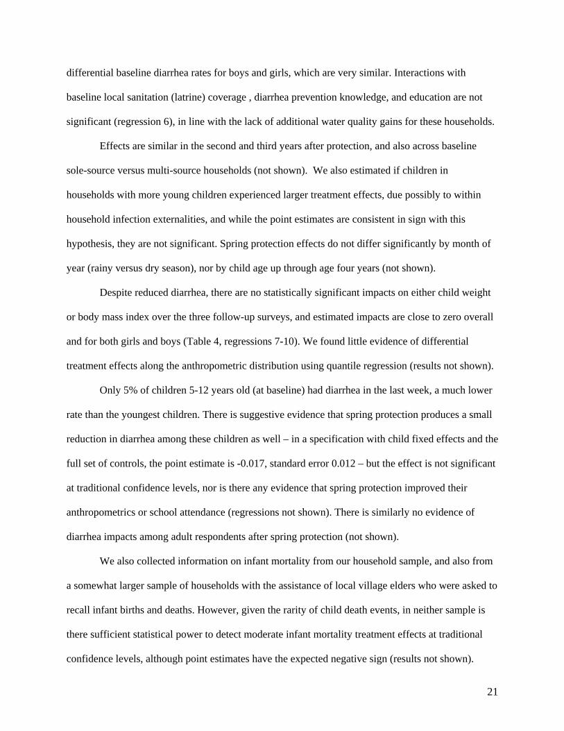
Despite reduced diarrhea, there are no statistically significant impacts on either child weight

or body mass index over the three follow-up surveys, and estimated impacts are close to zero overall

and for both girls and boys (Table 4, regressions 7-10). We found little evidence of differential

treatment effects along the anthropometric distribution using quantile regression (results not shown).

Only 5% of children 5-12 years old (at baseline) had diarrhea in the last week, a much lower

rate than the youngest children. There is suggestive evidence that spring protection produces a small

reduction in diarrhea among these children as well – in a specification with child fixed effects and the

full set of controls, the point estimate is -0.017, standard error 0.012 – but the effect is not significant

at traditional confidence levels, nor is there any evidence that spring protection improved their

anthropometrics or school attendance (regressions not shown). There is similarly no evidence of

diarrhea impacts among adult respondents after spring protection (not shown).

We also collected information on infant mortality from our household sample, and also from

a somewhat larger sample of households with the assistance of local village elders who were asked to

recall infant births and deaths. However, given the rarity of child death events, in neither sample is

there sufficient statistical power to detect moderate infant mortality treatment effects at traditional

confidence levels, although point estimates have the expected negative sign (results not shown).

22

7 Modeling water source choice

Estimating the impact of spring protection on water quality in the home and on health outcomes is

complicated by endogenous household behavioral responses to source water quality changes,

including the water source choice, and the decision of whether to use a point-of-use technology.

7.1 Estimating spring protection impacts on water source choice and behavior

The main behavioral change that resulted from spring protection is an increase in the use of the

protected springs for drinking water, while other behavioral changes appear to be minor (Table 5).

We split the data into two subsamples, sole-source users (those who only used the sample spring at

baseline) and multi-source users (those who also used other water sources): use of the protected

spring should increase more among multi-source users than sole-source users, since the latter group

have little or no room to increase usage. Assignment to spring protection treatment is strongly

positively correlated with use of the sample spring for those households not previously using it:

treated households are 21 percentage points more likely to use their sample spring as a source of

drinking water if they used other sources (multi-source users) at baseline (Table 5, Panel A). There

are similarly large impacts on the fraction of water collection trips made to the sample spring after

protection for multi-source users. Underlying this increased use of protected springs were

increasingly positive perceptions about the quality of drinking water from protected springs:

respondents at treated springs were 18 percentage points more likely to believe the water is “very

clean” during the rainy season, with somewhat smaller effects in the dry season.

There were small but statistically significant effects of spring protection on the average

distance households walked to their main drinking water source (average length was about 8 minutes

one-way or 16 minutes round-trip), with an effect of roughly one minute (Table 5, Panel A). A

possible explanation is that lines at springs are slightly shorter after protection (due to greater water

flow and easier collection), and that respondents mistakenly assign these time savings to reported

23

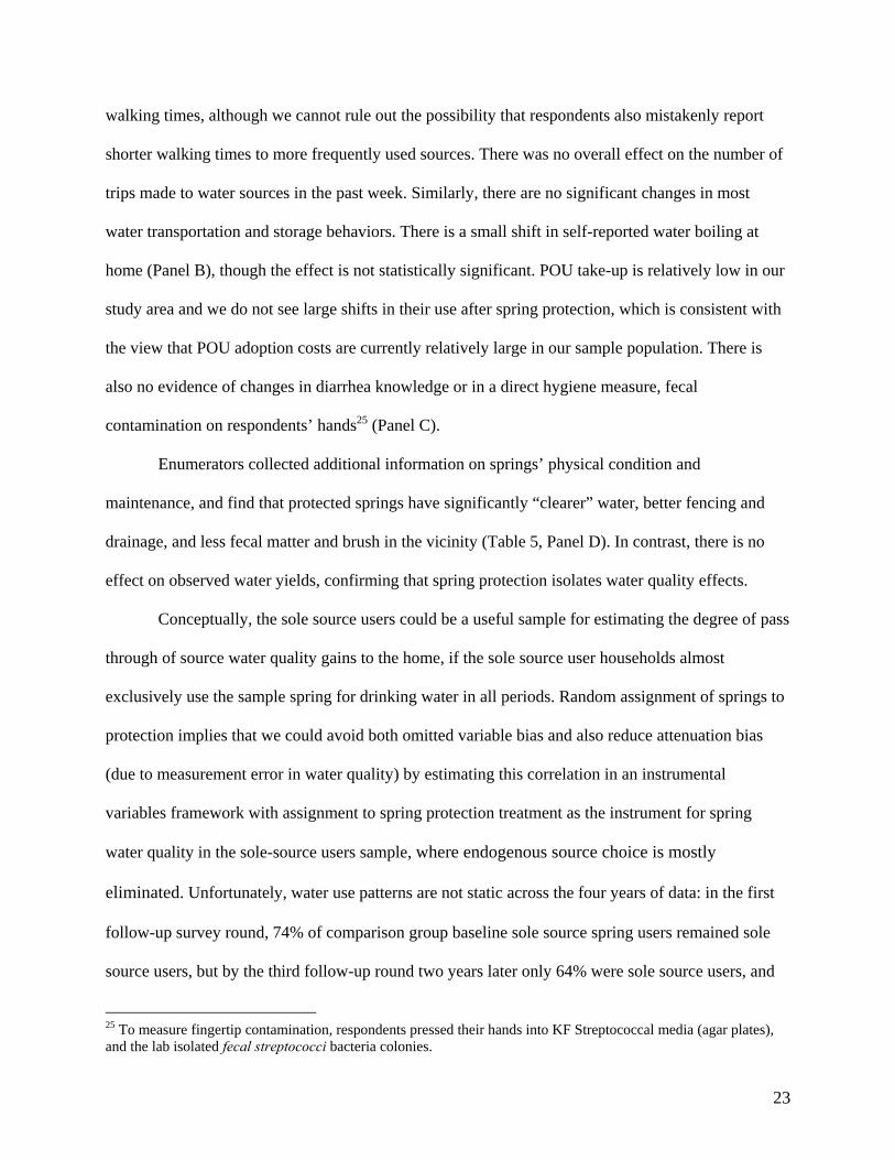
walking times, although we cannot rule out the possibility that respondents also mistakenly report

shorter walking times to more frequently used sources. There was no overall effect on the number of

trips made to water sources in the past week. Similarly, there are no significant changes in most

water transportation and storage behaviors. There is a small shift in self-reported water boiling at

home (Panel B), though the effect is not statistically significant. POU take-up is relatively low in our

study area and we do not see large shifts in their use after spring protection, which is consistent with

the view that POU adoption costs are currently relatively large in our sample population. There is

also no evidence of changes in diarrhea knowledge or in a direct hygiene measure, fecal

contamination on respondents’ hands25 (Panel C).

Enumerators collected additional information on springs’ physical condition and

maintenance, and find that protected springs have significantly “clearer” water, better fencing and

drainage, and less fecal matter and brush in the vicinity (Table 5, Panel D). In contrast, there is no

effect on observed water yields, confirming that spring protection isolates water quality effects.

Conceptually, the sole source users could be a useful sample for estimating the degree of pass

through of source water quality gains to the home, if the sole source user households almost

exclusively use the sample spring for drinking water in all periods. Random assignment of springs to

protection implies that we could avoid both omitted variable bias and also reduce attenuation bias

(due to measurement error in water quality) by estimating this correlation in an instrumental

variables framework with assignment to spring protection treatment as the instrument for spring

water quality in the sole-source users sample, where endogenous source choice is mostly

eliminated. Unfortunately, water use patterns are not static across the four years of data: in the first

follow-up survey round, 74% of comparison group baseline sole source spring users remained sole

source users, but by the third follow-up round two years later only 64% were sole source users, and

25 To measure fingertip contamination, respondents pressed their hands into KF Streptococcal media (agar plates), and the lab isolated fecal streptococci bacteria colonies.

24

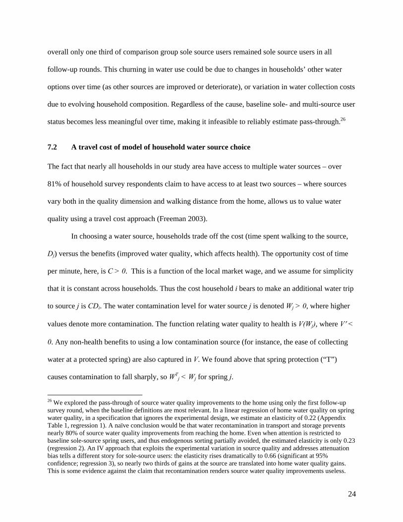
overall only one third of comparison group sole source users remained sole source users in all

follow-up rounds. This churning in water use could be due to changes in households’ other water

options over time (as other sources are improved or deteriorate), or variation in water collection costs

due to evolving household composition. Regardless of the cause, baseline sole- and multi-source user

status becomes less meaningful over time, making it infeasible to reliably estimate pass-through.26

7.2 A travel cost of model of household water source choice

The fact that nearly all households in our study area have access to multiple water sources – over

81% of household survey respondents claim to have access to at least two sources – where sources

vary both in the quality dimension and walking distance from the home, allows us to value water

quality using a travel cost approach (Freeman 2003).

In choosing a water source, households trade off the cost (time spent walking to the source,

Dj) versus the benefits (improved water quality, which affects health). The opportunity cost of time

per minute, here, is C > 0. This is a function of the local market wage, and we assume for simplicity

that it is constant across households. Thus the cost household i bears to make an additional water trip

to source j is CDi. The water contamination level for water source j is denoted Wj > 0, where higher

values denote more contamination. The function relating water quality to health is V(Wj), where V′ <

0. Any non-health benefits to using a low contamination source (for instance, the ease of collecting

water at a protected spring) are also captured in V. We found above that spring protection (“T”)

causes contamination to fall sharply, so WTj < Wj for spring j.

26 We explored the pass-through of source water quality improvements to the home using only the first follow-up survey round, when the baseline definitions are most relevant. In a linear regression of home water quality on spring water quality, in a specification that ignores the experimental design, we estimate an elasticity of 0.22 (Appendix Table 1, regression 1). A naïve conclusion would be that water recontamination in transport and storage prevents nearly 80% of source water quality improvements from reaching the home. Even when attention is restricted to baseline sole-source spring users, and thus endogenous sorting partially avoided, the estimated elasticity is only 0.23 (regression 2). An IV approach that exploits the experimental variation in source quality and addresses attenuation bias tells a different story for sole-source users: the elasticity rises dramatically to 0.66 (significant at 95% confidence; regression 3), so nearly two thirds of gains at the source are translated into home water quality gains. This is some evidence against the claim that recontamination renders source water quality improvements useless.

25

Household i’s indirect utility from a single water collection trip to source j can be represented

as Uij = V(Wj) – CDij. Household i chooses source j over an alternative source k if the benefits of its

water quality outweigh any additional travel costs, namely when {V(Wj) – V(Wk)} – C(Dij – Dik) ≥ 0.

More generally, in a context with multiple alternative water sources like our empirical setting, the

household chooses the source that maximizes utility over all water options in its choice set.

Focusing on those households on the margin between using the sample spring and an

alternative source conceptually allows one to estimate the value households place on spring

protection. Spring water quality improvements yield potential utility benefits of V(WjT) – V(Wj), and

travel costs would have to increase by the same amount to restore households to indifference. The

additional travel cost households are willing to incur is a revealed preference measure of their

willingness to pay (WTP) for improved water quality.

Other factors bring the model closer to the data. Most importantly, households make multiple

water collection trips and each trip is affected by unobserved factors, including the weather, the

expected queue, the direction an individual is walking for another task (i.e., to the market) or an

individual’s mood on a given day. Incorporating an i.i.d. error term eijt modeled as type I extreme

value, the indirect utility of a water collection trip to source j at time t is:

Uijt = V(Wjt) – CDijt + eijt (3).

More generally, given a set of characteristics Xijt for individual i and spring j at time t, where

controls include both the protection status of the local sample spring and the walking time to each

potential local alternative water source, as above, the probability household i chooses source j from

among all potential water source alternatives h ∈ H at time t can be represented by the usual

conditional logit formula (McFadden 1974):

∑ ′

′=

hiht

ijtijt

X

XXyP

)exp(

)exp()|(

β

β (4).

26

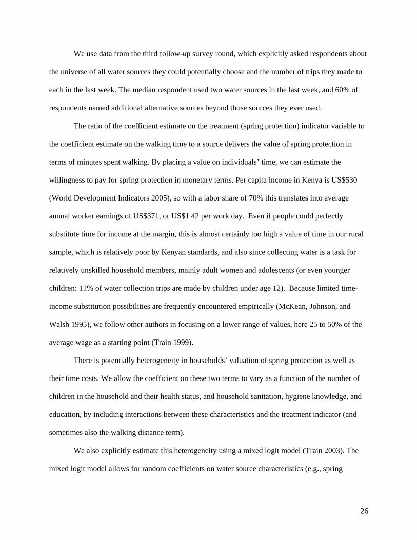
We use data from the third follow-up survey round, which explicitly asked respondents about

the universe of all water sources they could potentially choose and the number of trips they made to

each in the last week. The median respondent used two water sources in the last week, and 60% of

respondents named additional alternative sources beyond those sources they ever used.

The ratio of the coefficient estimate on the treatment (spring protection) indicator variable to

the coefficient estimate on the walking time to a source delivers the value of spring protection in

terms of minutes spent walking. By placing a value on individuals’ time, we can estimate the

willingness to pay for spring protection in monetary terms. Per capita income in Kenya is US$530

(World Development Indicators 2005), so with a labor share of 70% this translates into average

annual worker earnings of US$371, or US$1.42 per work day. Even if people could perfectly

substitute time for income at the margin, this is almost certainly too high a value of time in our rural

sample, which is relatively poor by Kenyan standards, and also since collecting water is a task for

relatively unskilled household members, mainly adult women and adolescents (or even younger

children: 11% of water collection trips are made by children under age 12). Because limited time-

income substitution possibilities are frequently encountered empirically (McKean, Johnson, and

Walsh 1995), we follow other authors in focusing on a lower range of values, here 25 to 50% of the

average wage as a starting point (Train 1999).

There is potentially heterogeneity in households’ valuation of spring protection as well as

their time costs. We allow the coefficient on these two terms to vary as a function of the number of

children in the household and their health status, and household sanitation, hygiene knowledge, and

education, by including interactions between these characteristics and the treatment indicator (and

sometimes also the walking distance term).

We also explicitly estimate this heterogeneity using a mixed logit model (Train 2003). The

mixed logit model allows for random coefficients on water source characteristics (e.g., spring

27

protection), in the indirect utility function. Simulation techniques are used since there is typically no

closed-form solution. We estimate choice probabilities as

βββ

ββ

dfX

XXyP

hiht

ijtijt )(

)exp(

)exp()|( ∫

∑ ′

′= (5).

where y, X and β are defined as above, and f(⋅) is the mixing distribution, which we take to be the

normal distribution for the coefficient on spring protection in our application. Numerical methods

allow us to maximize the log-likelihood to estimate the mean and standard deviation of β.

7.3 Estimating households’ willingness to pay for cleaner water

Respondents report that springs are the main source of water in this area: nearly three quarters of all

water collection trips are to springs (either unprotected or protected). The next most common source

are wells (at 13%), followed by smaller numbers of water collection trips to boreholes (7%),

rivers/streams (4%), lakes, ponds, and other sources. The bulk of collection trips are for drinking

water: 81% of water collection trips are to sources the respondents used for drinking water in the last

week.27 We focus on water collection trips to all sources, even those not listed as drinking water

sources, since there is likely misreporting of water uses (especially when the respondent herself does

not drink the water from a particular source but other household members might). We also focus

on all water trips for internal consistency: our stated preference valuations below are derived

from questions that ask about all water source trips, not just those for drinking water.

The conditional logit analysis yields a large, negative and statistically significant effect on the

round-trip walking distance to water source (measured in minutes) term, at -0.058 (standard error

0.007, Table 6, regression 1) and a positive statistically significant effect on the treatment (protected)

27 This does not imply that 81% of total water consumption is for drinking, since household members often wash clothes and bathe at the water sources themselves.

28

indicator term (0.56, standard error 0.21). Other terms in the regression indicate that streams and

rivers are less preferred sources relative to the omitted category (non-program springs), while there is

no clear preference among program (sample) springs, non-program springs, wells and boreholes.

One concern with the interpretation of this result is possible measurement error in the

reported distance walking variable. The correlation across survey rounds in the reported walking

distance to the sample spring is moderate at 0.38, so attenuation bias could be large. In addition to

simple recall error, the variation in reported walking time may be due to actual variation in travel

time, depending on the weather, what else the individual is carrying to the source (e.g., carrying a

baby, goods for market), and the respondent’s health or energy level that day. To approximately

correct for classical measurement error in this term, we inflate its coefficient to -0.058 / 0.38 = -0.153

and use this correction in valuation calculations below.28

The ratio of the two main coefficient estimates in this specification implies that one round

trip to a protected spring compared to an unprotected spring is valued at (0.56)/(0.153) = 3.7 minutes

of walking time. Over the course of a year, using the average number of trips per week to the sample

spring, this is equivalent to roughly 13 work days, a figure independent of the assumed price of time.

This is a reasonably large effect: if household members’ time is valued at 50% of the Kenyan average

wage, or US$0.71 per work day (US$0.0015 per minute), and households make our sample average

of 32 water collection trips per week to the sample spring (about two thirds of total water collection

trips), 52 weeks per year, the total average value to these households from protection is (3.7

minutes)*(US$0.0015/minute)*(32 trips/week)*(52 weeks/year) = US$9.05 per year (Table 7, Panel

A). At the arguably more realistic time value of 25% of the wage ($0.35 per work day), household

willingness to pay for spring protection is only US$4.52 per year. Since there are on average seven

members per household, this is a valuation of roughly US$1 per capita per year.

28 The attenuation bias correction estimated in a Monte Carlo simulation is similar, at roughly 0.3 (not shown).

29

The availability of two waves of spring protection (in early 2005 versus late 2005) allows us

to assess whether households’ valuation changes with greater exposure to the protected spring, but

valuations are nearly identical for those households who had one additional year of experience with

spring protection (results not shown).

Combining the results from Tables 4 and 6 sheds light on the WTP to avert child diarrhea.

The average number of averted diarrhea cases due to spring protection is (-0.047 cases / child-week)

* (2.2 children under age 3 / household) * (52 weeks / year) = -5.4 diarrhea cases per household-year.

Using our spring protection household WTP range of US$4.52-9.05 per year, this translates into

US$0.84-1.68 per case of diarrhea averted, under the assumption that all of spring protection’s value

works through child health gains.

These valuation figures lie below estimated costs per case of diarrhea averted with several

common interventions, like handwashing (Varley et al. 1998). Thus it appears many households in

our sample would not be willing to pay for spring protection and other water, hygiene and sanitation

interventions if their benefits come mainly in the form of reduced child diarrhea.

A different assumption, namely, that household WTP is driven entirely by reduced child

mortality risk, allows us to estimate the value these households place on their children’s lives using

our revealed preference methodology. There are approximately 5.69 deaths per 1000 children under

age 5 each year in Sub-Saharan Africa (Lopez et al. 2006, Table 3B.7), and roughly 4.9 annual

diarrhea episodes per African child under age 5, based on the findings in Kirkwood (1991), who

reviews 100 longitudinal studies of diarrheal disease in 33 African countries . If each diarrhea

episode averted (by better quality water) reduced mortality risk by an equal amount, then this

translates into 1.16 deaths from diarrhea averted for each 1000 diarrhea cases eliminated. The value

of averting one child diarrhea death among these households thus ranges from US$725 to US$1451.

These values are far below the estimated value of a statistical life in the U.S. and other rich countries

(using hedonic labor market approaches), where the median value is approximately US$7 million

30

(Viscusi and Aldy 2003). Studies from two poorer countries (India and Taiwan) yield estimates on

the order of US$0.5-1 million per statistical life, although they are difficult to compare to our sample

since they rely on data for urban factory workers in those countries, who are much richer than our

poor rural respondents. We are unaware of hedonic value of statistical life estimates from Africa.

To the extent that spring protection yields other non-health benefits as well, these estimates

would be upper bounds on the willingness to pay to avoid diarrhea cases or deaths. However, while

the non-health benefits of spring protection – in terms of water appearance, taste or ease of water

collection – could theoretically contribute to willingness to pay, we find no evidence that these have

a significant effect on WTP in practice. The inclusion of terms for measured E. Coli contamination

available at a subset of alternative water sources, as well as the household’s perception of water

quality at each source, reduces the coefficient estimate on the spring protection treatment indicator

near zero (Table 6, regression 2). Thus the bulk of the valuation appears to come from the water

quality benefits rather than other amenities associated with spring protection.

Theoretically, households with young children should have both greater time costs of

walking to collect water (due to the demands of child care and difficulty carrying a small child) and

also greater benefits of clean water, since the epidemiological evidence suggests that young children

experience the largest health gains from improved water quality. Empirically, we find that

households with more children under age 5 at baseline find additional walking distance to a source to

be more costly, and this effect is especially strong for households who had young children with

diarrhea at baseline: that effect is large and statistically significant at 99% confidence (Table 6,

regression 3). The interaction of 0-5 year old children diarrhea with the treatment indicator is large

and positive, suggesting that households with sick children also place somewhat greater value on

cleaner water, and on net the two effects nearly cancel out.

Household valuation for spring protection is not significantly higher as a function of diarrhea

prevention knowledge (Table 6, regression 4), nor does household knowledge of the link between

31

contaminated water and diarrheal disease in particular affect the value placed on spring protection

(not shown). There is some evidence it rises with latrine ownership and with mother’s years of

schooling, although the latter interaction effect is very small (regression 4). Neither child gender nor

asset ownership significantly affect households’ taste for spring protection (not shown).

Using the mixed logit approach, we find only moderate dispersion of spring protection

valuations in our sample of households: the mean coefficient estimate on the spring protection

indicator remains unchanged at 0.56, with a standard deviation of 0.11 (standard error 0.04, Table 6,

regression 4), assuming normally distributed valuations. The mean and standard deviation of

household willingness to pay for spring protection based on these revealed preference mixed logit

results are presented in Table 7, Panel A, for a variety of time values.

Stated Preference Water Valuations

The first stated preference valuation approach is a stated ranking measure. Here, rather than relying

on information on actual household water trips, we instead ask respondents to rank order their

potential water source options. This is done sequentially in the survey, with the highest ranked source

eliminated from the choice set at each subsequent question. These data are then used in a travel cost

discrete choice analysis nearly identical to the revealed preference regressions.

Estimated stated preference ranking willingness to pay for spring protection is much higher

than the revealed preference estimates. The magnitude of the coefficient estimate on distance

walking falls to -0.033 while that on spring protection rises to 0.96 (Table 6, regression 6). Using the

same attenuation bias correction as above, the WTP for one year of spring protection, using time

valued at 50% (25%) of the average Kenyan wage, is US$26.19 (US$13.09). This is almost exactly

three times greater than the revealed preference values (Table 7, Panel B).

Comparing the analogous columns in Table 6 (regressions 1 and 6) also highlights interesting

reporting patterns in the stated preference ranking case. The coefficient estimates on several

32

unimproved sources many Kenyans generally think of as “bad” or unclean (e.g., streams, rivers,

lakes, ponds) are far more negative in the stated preference ranking regression than in the revealed

preference case, while the coefficient estimate on spring protection is more positive. This suggests

social desirability bias may be playing a role in some respondents’ stated preference rankings.

We also find considerably larger dispersion in stated preference valuations for spring

protection than in the analogous revealed preference mixed logit estimates, with standard deviations

three times larger (Table 7, Panel B). One plausible explanation for the dispersion is that many

respondents fail to introspect carefully in this hypothetical exercise, and thus their resulting answers

are far “noisier” than in the revealed preference case, where they face real (time) budget constraints.

The second stated preference method is contingent valuation. Here households in protected

spring communities were asked how much they would be willing to pay to keep their spring

protected. The contingent valuation questions were only asked of households in the treatment group

since they have first-hand experience with spring protection. In the final wave of the survey,

respondents were first asked if they would be willing to pay either 250 or 500 Kenyan Shillings,

followed by the question that emphasized the expenditure trade-off for their assigned amount (in

other words, what goods they would be giving up by spending that much on spring protection), and

then were asked if they would be willing to pay the next higher amount also with emphasis on the

expenditure trade-off. This closed-end format, offering discrete value choices, is standard in the

contingent valuation literature (Bateman and Willis 1999).The question wording was:

Now that you have seen the protected spring, suppose that somehow the spring had been split so that there was free access to an unprotected spring and restricted access to a protected spring, both at the same site. Would you be willing to pay _____ Ksh for one year's access to the protected spring, assuming everyone else would also have to pay this amount too?29

29 The wording of the question emphasizing expenditure trade-offs was: “So, just to be sure I understand, you would be willing to give up [say price from name list for this specific household] Ksh of purchases that you currently make in order to have access to the protected part of the spring. 250 Ksh per year is about 20 Ksh every month. That's a little bit less than a half-liter of kerosene or a quarter-kilo of sugar every month. For another reference, a school uniform costs about 500 Ksh. If you had to give up something you would otherwise spend money

33

The main finding is that nearly all households claim to be willing to pay US$7.14 for one

year of spring protection, and the majority of households are willing to pay twice that (US$14.29)

even after being walked through the expenditure trade-offs by the enumerator (Table 7, Panel C). The

use of the expenditure trade-off prompt reduces willing to pay substantially (by 11-14 percentage

points), indicating that the contingent valuation results are sensitive to survey question framing.

If we assume spring protection valuations are normally distributed, the distribution that best

fits the contingent valuation response data (using maximum likelihood) has mean willingness to pay

of US$17.64 (standard deviation US$13.09, Table 7, Panel C). This is considerably more than our

best revealed preference estimates of US$4.52-9.05 per year, but lies within the range of plausible

stated preference ranking valuations discussed above (US$13.09-26.19).

Another piece of evidence on the sensitivity of the contingent valuation approach to framing

is the divergence in valuations as a function of the monetary starting value: those respondents

randomly chosen to be asked whether they valued a year of spring protection at 500 Kenyan Shillings

have mean willingness to pay that is twice as high ($23.91) as those respondents first asked about a

value of 250 Kenyan Shillings ($12.62), perhaps because the proposed starting value implicitly

contains some information for respondents about what a “reasonable” valuation should be.

We can pin down an exact value of water collector’s time by assuming that the mean WTP

for spring protection is equated under both stated preference approaches (stated preference ranking

and contingent valuation).30 This yields a mean revealed preference WTP of US$5.79 (with standard

deviation US$3.05) for one year of protection. The estimated WTP distributions for the three

valuation approaches under this assumption (Figure 4) indicate that stated preference methods

on, would you still be willing to pay _____ Ksh [price for this household] for access to the protected part of the spring?” We thank Michael Hanemann for discussions on the phrasing and framing of these questions. 30 We thank Enrico Moretti for this suggestion.

34

exaggerate household willingness to pay for environmental amenities in a rural Kenyan setting, and

that the more reliable revealed preference approach yields more modest and less variable valuations.

8. The provision of clean water under alternative policies and institutions

The Social Returns to Spring Protection

Current Kenyan law and custom prevent landowners from charging local spring users for water.

Perhaps partially as a result of these weak private property rights, virtually no springs are privately

protected in our study area, despite the identified health gains. In this section we use the valuation

estimates derived above to determine the socially optimal level of spring protection.

We begin by assessing the socially optimal degree of spring protection in this region. Spring

protection costs about US$1000 per spring and lasts for at least ten years, with maintenance costs of

around US$55 per year, leading to a discounted net present cost of US$1480 (with a 5% annual

discount). Under the assumption that the deadweight loss from tax distortions is roughly 0.3 of the

revenue raised (Ballard et al 1985), the total social cost would be US$1924.

At this level of construction and maintenance costs, the social rate of return of spring

protection appears negative. If households are willing to pay $5.79 per year and, as in our baseline

data, 31 households use the typical spring, the net present value of WTP for spring protection is only

US$1386. (This figure abstracts away from the utility gains associated with additional users starting

to use protected springs, something we will incorporate in future work). The fact that spring

protection has negative social returns on average could be a partial explanation for the low rates of

spring protection in the region. Returns to spring protection will be larger as the number of

households with young children using a spring grows – for instance, in more densely populated rural

areas, or in towns and cities. If the average number of spring users rose by a third to 43 households

per spring, average social returns would become positive in our setting.

35

The relevant decision for some policymakers may not be spring protection versus doing

nothing, but rather investing in spring protection versus other interventions to improve water quality

and ultimately child health. We next compare the diarrhea reduction cost-effectiveness of spring

protection versus a point-of-use (POU) water treatment, at-home chlorination, also introduced in our

study sample. The reduction in diarrhea incidence among children under age three from introducing

POU treatment was about 45%, double the effect from spring protection.31 This is an intention to

treat (ITT) estimate, and POU take-up was about 54%, so treatment effects on the treated were

extremely large for POU users. The obvious implication is that larger reductions in water

contamination (from POU treatment) are more effective at reducing diarrhea than moderate water

improvements such as those achieved from spring protection.32

These estimates allow us to compare the child health benefits associated with spring

protection versus the reductions in diarrheal morbidity that could have been realized had the

approximately US$148,000 spent to protect the 100 treatment springs in our sample and maintain

them for ten years, instead been spent providing POU products to households with young children. In

our study area, a one month’s supply of the in-home chlorination product (called WaterGuard

locally) can be purchased for roughly $0.29 (20 Kenyan Shillings).

We begin by noting that 19% of comparison children under age three in our sample are

reported having diarrhea in the past week across all survey rounds. All other things equal, and

assuming constant size of the under-three age cohort, this implies 837,132 cases at households that

use sample springs over the ten years that a spring might last and (837,132) * (0.047/0.19) = 207,080

cases averted as a result of the intervention. This implies a cost per diarrhea case averted of US$0.71.

31 A fuller presentation of these POU results is contained in related research (Kremer, Miguel, Null, and Zwane 2007). In future work we will also estimate if POU technologies are most effectively employed as complements or substitutes for source water improvements like spring protection. 32 In a near-by setting but using a different and more intensive method of measuring diarrhea, Crump et al. (2005) estimate that the effect of point of use water treatment is a reduction in diarrheal prevalence per 100 weeks of about 17 percent, similar to the reduction we estimate for source water quality improvements. This impact estimate is for children under two and in a setting where high take up led to 78% of treatment households with E. coli MPN <1.

36

We can also calculate the number of Disability Adjusted Life Years (DALYs) averted by

spring protection, using the standard WHO approach.33 This calculation is a function of the average

length of a diarrhea episode, and the number of deaths that occur per 1000 diarrhea cases. An

ongoing high-frequency data collection effort, in which we collect morbidity diaries, indicates that

average diarrhea episode length in our sample is 6.5 days. With 1.16 deaths per 1000 cases of

diarrhea (as discussed above), spring protection averts 207,080 DALYs, a cost of US$189 per DALY

averted. Of course, this is an underestimate of spring protection’s health benefits to the extent there

are some benefits for people over age three.

If the chlorine POU product were given to every household with children under age three in

our sample (about 80% of homes) for ten years, this would cost $65,657 in current dollars using a

time discount rate of 5%. The cost per case of diarrhea averted with WaterGuard is thus about $0.17,

and so four times as many cases could be averted by focusing on point-of-use treatment products

instead of spring protection. Of course, this assumes that a 54% take-up rate could be sustained over

ten years and that the delivery mechanism could perfectly target the 80% of households that have

children under age three. Still, any long-run POU take-up rate above about 13% would result in in-

home chlorine treatment being more cost-effective than spring protection at reducing diarrhea.

Conclusions about the cost-effectiveness of the POU technology are sensitive to its price. The

current price of WaterGuard in local markets in Kenya is heavily subsidized by the organization

marketing the product: the price covers production and distribution costs but marketing costs are

fully subsidized. Yet POU chlorination costs would be much lower if chlorine were distributed in

bulk, without the marketing, packaging, and retail distribution costs for the small bottles of the

product sold in Kenyan shops. The local cost of a similar chlorine product, bleach for washing,

distributed in much larger containers is only 27% of the cost of WaterGuard per unit of chlorine. If

the cost of POU chlorine were reduced, the cost per diarrhea case averted would be $0.05 and point- 33 For more information on the DALY concept, see: http://www.who.int/healthinfo/boddaly/en/index.html.

37

of-use treatment would be 14 times more cost effective than spring protection at averting diarrhea

cases. The retail model, where the cost of packaging far exceeds the cost of the POU product, thus

appears to greatly reduce the relative cost-effectiveness of in-home chlorination.

Spring protection is more cost effective the greater the number of households that benefit

from the intervention, so as population density increases source water quality investments could be

increasingly cost-effective. Assuming the current retail price of WaterGuard, source spring protection

becomes more cost-effective than point-of-use water treatment when there are at least 127 household

users per spring. While very high for our rural study area, this usage level is certainly possible in

urban and peri-urban areas. Improving source water quality is more likely to be an appropriate policy

in areas with denser population and fewer alternative sources, leading to many users per spring.

Privatization Policy Simulations

One potential policy option in the rural water sector is privatization, allowing land owners to charge

households for access to spring water on their land. The resulting profits could provide an incentive

for spring owners to invest in protection. A downside would be the static distortion introduced by

pricing spring water above its marginal cost of zero.

We simulate the following game. In t=0, the property rights regime is chosen. The two

potential cases are the “status quo” – which is characterized by spring water prices of zero and no

spring protection – and “privatization”. In the latter case, landowners decide whether or not to protect

their spring (in t=1), and then set a non-negative price per unit of water collected (t=2). Finally, in

t=3, households make their water collection choices, where these are governed by the revealed

preference coefficients estimated in the mixed logit specification above (Table 6, regression 5).

Given local demand, spring owners maximize profits, which are equivalent to revenues

minus any spring protection construction and maintenance costs, since the marginal cost of spring

38

water provision is zero. In practice, we find this price level through a grid search over a wide range

of non-negative prices. Spring owners optimize over a ten year period (the same time horizon used in

the social planner’s problem above). In the status quo case, households make water consumption

choices given there is no spring protection and a water price of zero.

We allow spring resources to be privatized but not other source types. This is a natural policy

in our setting: it is difficult to restrict access to natural rivers, streams, ponds and lakes, and many

wells – especially boreholes – are sunk on public property, including school grounds or market

centers, where the landowner is not clearly defined. We do not allow spring owners to engage in

price discrimination since easy resale in rural settings makes it unlikely to succeed, and also abstract

from possible collusion among spring owners.

We first focus on the simplest case, where each sample spring owner is operated as a

monopolist; we will extend the analysis to consider competition among landowners in future work.34

In a preliminary analysis, we find that 22% of spring owners find it profit-maximizing to protect their

spring, given local water demand conditions. A particularly interesting subsample to consider are

springs with at least 43 user households at baseline, since in this case our valuation figures indicate

that spring protection is socially optimal. Yet among the 30 springs with at least 43 baseline users,

only six, or 20%, choose spring protection.

The average annual price charged per household in these springs ranges from US$1.65-4.12,

a non-trivial amount for these households. Over all springs, 79% of households have lower utility in

the privatization case than under the status quo, and the sum of utility across all households is also

lower. Even among the springs with at least 43 baseline users, 78% of households “lose” from

privatization. In this analysis, the privatization of spring water resources appears only moderately

34 We currently consider demand only among baseline spring user households, yet one important factor in determining total water demand is the extent to which new users (who did not use the spring at baseline) shift to using the spring. We are currently conducting detailed household censuses in the vicinity of a subset of sample springs to determine the increase in demand from new users, and will incorporate this into future versions.

39

effective at reaching socially efficient levels of water infrastructure investment, and has adverse

distributional consequences, with large rents for land owners – who are now able to charge positive

prices for water – and losses for the vast majority of consumers.

Spring protection rates remain relatively low in the monopoly case, in part, because land

owners are able to charge positive prices for water even from unprotected springs, capturing

considerable consumer surplus even in that case. Thus in most cases it is not profit-maximizing to

incur additional spring protection and maintenance expenses. A modified privatization policy would

only permit spring owners to charge positive water prices if they have invested in spring protection.

This simulation yields much higher rates of investment: now 62% of spring owners find it

profit maximizing to invest to spring protection. Yet protection rates actually appear too high: most

land owners choose to protect their spring even when there are fewer than 43 household users – in

other words, when protection is not socially optimal – in part because protection allows spring

owners to capture additional rents. While this policy still leaves most households worse off than the

status quo, it is marginally better for household welfare than the original privatization simulation:

only 53% of households experience utility losses from this modified form of privatization.

9. Discussion and conclusion

Spring protection dramatically improved source water quality in a rural African setting, reducing

contamination by two thirds on average and home water contamination by nearly one quarter. Child

diarrhea fell by roughly one quarter, although source water protection appears less cost-effective than

a point-of-use treatment at reducing child diarrhea.

An interpretation common in the existing water literature is that source water quality

improvements only translate into home water quality gains – and eventually child health gains –

when there are good household hygiene practices and adequate local sanitation already in place.

However, we do not find any evidence that spring protection led to larger home water quality gains

40

when hygiene knowledge or latrine coverage were better. Also, spring protection did not lead to any

detectable changes in water collection, transport, or storage practices, water quantity used, or to

changes in any other preventive health behaviors that we measured. However, there were sharp

changes in water source choices among some households.

We estimate willingness to pay for improved water by analyzing these shifting household

water choices – and in particular, the distance they are willing to walk for water – in response to

spring protection. We find moderate household valuation for spring protection, on the order of

US$4.52-9.05 per household annually. This translates into a household willingness to pay of

approximately US$0.84-1.68 per averted case of child diarrhea. Under the assumption that all of this

valuation is driven by reduced child mortality risk, households appear willingness to pay US$725-

1451 per child life saved. In contrast, stated preference valuation approaches produce estimated WTP

estimates higher than these by as much as three times, and with much greater dispersion in reported

valuations, which raises questions about the reliability of these methods in settings like ours.

Reference

Angrist, J. et al. (1996), “Identification of causal effects using instrumental variables,” Journal of the American Statistical Association 91(434), 444-472.

Aziz, K., B. Hoque, K. Hasan, M. Patwary, S. Huttly, M. Arman, and R. Feachem (1990), “Reduction in diarrhoeal diseases in children in rural Bangladesh by environmental and behavioural modifications,” Transactions of the Royal Society of Tropical Medicine and Hygiene 84(3), 433-438.

Ballard, Charles L., John B. Shoven, and John Whalley. (1985). “General Equilibrium Computations of the Marginal Welfare Costs of Taxes in the United States”, American Economic Review, 75(1), 128-138.

Bateman, I. and K. G. Willis, (1999), Valuing Environmental Preferences: The Theory and Practice of the Contingent Valuation Method in the US, EU and Developing Countries. Oxford University Press: New York.

Beaton, G.H. et al. (1993), “Effectiveness of vitamin A supplementation in the control of young child mortality in developing countries,” Nutrition Policy Discussion Paper #13 ACC/SCN: Geneva.

41

Black, R.E. (1998), “Therapeutic and preventive effects of zinc on serious childhood infections diseases in developing countries,” American Journal of Clinical Nutrition 68(supplement), 476s-9s.

Blum, D. and R.G. Feacham (1983), “Measuring the impact of water supply and sanitation investments on diarrheal diseases: Problems of methodology,” International Journal of Epidemiology 12(3), 357-65.

Bryce, J. et al. (2005), “WHO estimates of the causes of death in children,” Lancet 365: 1147-52.

Carson, R.T., N.E. Flores, K. Martin, and J. Wright (1996), Contingent valuation and revealed preference methodologies: Comparing the estimates for quasi-public goods, Land Economics,72(1): 80-99.

Choe, K. (1996) “The economic benefits of surface water quality improvements in developing countries: A case study of Davaeo, Philippines” Land Economics 72(4): 519-537

Crump JA, Otieno PO, Slutsker L et al. (2005) “Household based treatment of drinking water with flocculant-disinfectant for preventing diarrhoea in areas with turbid source water in rural western Kenya: cluster randomised controlled trial,” British Medical Journal, 331, 478–483.

Diamond, P.A and J. A. Hausman, (1994), “Contingent valuation: Is some number better than no number?” Journal of Economic Perspectives, 8(4),45-64

Esrey S.A. (1996), “Waste, water and well-being: A multicountry study,” American Journal of Epidemiology 143(6), 608-22.

Esrey S.A. et al. (1991), “Effects of improved water supply and sanitation on ascariasis, diarrhea, dracunculiasis, hookworm infection, schistosomiasis and trachoma,” Bulletin of the World Health Organization 60, 609-621.

Esrey S. A. et al. (1985), “Interventions for the control of diarrheal diseases among young children: Improving water supplies and excreta disposal facilities,” Bulletin of the World Health Organization 63(4), 757-72.

Esrey S. A. and J.-P. Habicht (1986), “Epidemiologic evidence for health benefits from improved water and sanitation in developing countries,” Epidemiology Review 8, 117-128.

Feacham, R.A. (1977), Water supplies for low-income communities: Resource allocation, planning and design for a crisis situation, in R. Feacham, M. McGarry, and D. Mara eds., “Waste, water, and health in hot climates,” John Wiley and Sons: London.

Fewtrell, L. et al. (2005), “Water, sanitation, and hygiene interventions to reduce diarrhoea in less developed countries: A systematic review and meta-analysis,” Lancet Infectious Diseases 5, 42-52.

Freeman, A. M. III. 2003. The Measurement of Environmental and Resource Values: Theory and Methods (Second Edition). Washington DC: Resources for the Future.

Glass, R. et al. (2004), Rotavirus vaccines, in C.A. de Quadros, ed., “Vaccines: Preventing Disease & Protecting Health,” Pan American Health Organization: Washington, D.C.

42

Griffin, C. et al (1995) “Contingent valuation and actual behavior: predicting connections to new water systems in the state of Kerala, India” World Bank Economic Review 9(3): 373-395

Grotto, I. et al. (2003), “Vitamin A supplementation and childhood morbidity from diarrhea and respiratory infections: A meta-analysis,” Journal of Pediatrics 142, 297-304.

Hill, Z. et al. (2004), Family and community practices that promote child survival, growth, and development: A review of the evidence, WHO: Geneva.

Huttly S.R.A. et al. (1987), “The epidemiology of acute diarrhea in a rural community in Imo State, Nigeria,” Transactions of the Royal Society of Tropical Medicine and Hygiene 81, 865-70.

Iyer, Param, Jennifer Davis, Elif Yavuz and Barbara Evans (2006), “Rural water supply, sanitation, and hygiene: A review of 25 years of World Bank lending (1978–2003),” World Bank Water Supply & Sanitation Working Notes, Note No. 10, July 2006.

Kirkwood, B.R. (1991). “Diarrhea”, pp. 134-157, in R.G. Feacham and D.T. Jamison, eds.,

Disease and Mortality in Sub-Saharan Africa. New York: Oxford University Press for World Bank.

Lenehan, A. and J. Martin (1997), “Spring protection in southern KwaZulu Natal,” Paper presented at the twenty-third Water, Engineering, and Development Centre (WEDC) Conference on Affordable Water Supply and Sanitation, Durban.

Loewenstein, George, Ted O’Donoghue, and Matthew Rabin. (2003). “Projection Bias in Predicting Future Utility”, Quarterly Journal of Economics, 118(4), 1209-1248.

Lopez, A.D., et al., eds. (2006). Global Burden of Disease and Risk Factors, Washington DC: World Bank and Oxford University Press.

McFadden, D. (1974), “Conditional logit analysis of qualitative choice behavior”, in P. Zarembka, ed., Frontiers in Econometrics, Academic Press, New York, pp. 105-142.

McKean, J. R., D. Johnson, and R. Walsh, (1995) "Valuing time in travel cost demand analysis: An empirical investigation," Land Economics, 71(1).

Miguel, E., and M. K. Gugerty. (2005). “Ethnic diversity, social sanctions, and public goods in Kenya”, Journal of Public Economics, 89(11-12), 2325-2368.

Miller, P. and N. Hirschhorn (1995), “The effect of a national control of diarrheal diseases program on mortality: The case of Egypt,” Social Science Medicine 40(10), 1-30.

Mintz, Eric, Jamie Bartram, Peter Lochery and Martin Wegelin, (2001), “Not just a drop in the bucket: Expanding access to point-of-use water treatment systems,” American Journal of Public Health, October; 91(10): 1565–1570.

Mu, X., D., Whittington, and J. Briscoe, (1990), “Modelling village water demand behavior: A

discrete choice approach,” Water Resources Research 26(4), 521-529.

43

Mumma, Albert. (2005). “Kenya’s new water law: an analysis of the implications for the rural poor”, paper presented at the Workshop on African Water Laws: Plural Legislative Frameworks for Rural Water Management in Africa, 26-28 January 2005, Johannesburg, South Africa.

Mwami, J. (1995), “Spring protection- sustainable water supply,” Paper presented at the twenty-first Water, Engineering, and Development Centre (WEDC) Conference on Affordable Water Supply and Sanitation, Kampala.

Pinfold J.V. (1990), “Faecal contamination of water and fingertip prints as a method for evaluating the effect of low-cost water supply and sanitation activities on faeco-oral disease transmission. A case study in rural north-east Thailand,” Epidemiology and Infection 105, 363–375.

Perera, B.J.C. et al. (1999), “The impact of breastfeeding practices on respiratory and diarrhoeal disease in infancy: A study from Sri Lanka,” Journal of Tropical Pediatrics 45, 115-8.

Phaneuf, D. and V.K. Smith (2003), Recreation demand models, in “Handbook of Environmental Economics,” K. G. Mäler and J. R. Vincent eds., Volume 2, pages 671-761 Elesevier: Amsterdam

Raisler, J. et al. (1999), “Breastfeeding and infant illness: A dose-response relationship?” American Journal of Public Health 89, 25-30.

Ramakrishnan, U. and R. Matorell (1998), “The role of vitamin A in reducing child mortality and morbidity and improving growth,” Salud Publica de Mexico 40(2), 189-198.

Rosado, Maria et al (2006) “Combining averting behavior and contingent valuation data: an application to drinking water treatment in Brazil” Environment and Development Economics, 11:729-746

Rosen, S. and J.R. Vincent (1999), “Household water resources and rural productivity in Sub-Saharan Africa: A review of the evidence,” Harvard Institute for International Development Discussion Paper # 673.

Train, K., “Mixed Logit Models of Recreation Demand,” in C. Kling and J. Herriges, eds., Valuing the Environment Using Recreation Demand Models, Elgar Press, 1999.

Train, K. E. (2003). Discrete Choice Methods with Simulation. Cambridge: Cambridge.

Unicef (2006), “Meeting the MDG Drinking Water and Sanitation Target: A Mid-Term Assessment of Progress,” Available at: http://www.unicef.org/wes/mdgreport/index.php

UNEP (United Nations Environment Program) (1998), Sourcebook of alternative technologies for freshwater augmentation in Africa, Osaka: UNEP.

USAID (United States Agency for International Development) (1996), Environment, health and people, An update on USAID’s Environmental Health Project: Arlington VA.

Varley, R.C.G. et al. (1998), “A reassessment of the cost-effectiveness of water and sanitation interventions in programmes for controlling childhood diarrhea,” Bulletin of the World Health Organization 76(6), 617-631.

44

Vaz, L., and P. Jha (2001), “Note on the health impact of water and sanitation services,” WHO Commission on Macroeconomics and Health Working Paper Series Paper #WG5: 23.

Victora, C.G. et al. (2000), “Reducing deaths from diarrhea through oral rehydration therapy,” Bulletin of the World Health Organization 78(10), 1246-56.

Viscusi, W. Kip, and Joseph E. Aldy. (2003). “The Value of a Statistical Life: A Critical Review of Market Estimates Throughout the World”, Journal of Risk and Uncertainty, 27(1): 5-76.

UN-Water/Africa (2006), African Water Development Report, Economic Commission for Africa: Addis Ababa, Ethiopia.

Watson, T. (2006), “Public health investments and the infant mortality gap: Evidence from federal sanitation interventions and hospitals on U.S. Indian Reservations,” Journal of Public Economics, 90(8-9), 1537-1560.

Wooldridge, Jeffrey M. (2002). Econometric Analysis of Cross-section and Panel Data, MIT Press, Cambridge.

WHO (World Health Organization) (2000), Global water supply and sanitation assessment, WHO: Geneva.

WHO (World Health Organization) (2002a), Managing water in the home: Accelerated health gains from improved water supply, WHO: Geneva.

WHO (World Health Organization) Collaborative Study Team on the Role of Breastfeeding on the Prevention of Infant mortality (2000), “Effect of breastfeeding on infant and child mortality due to infectious diseases in less developed countries: A pooled analysis,” Lancet 355, 451-5.

Whittington, D., X. Mu, and R. Roche (1990) “Calculating the value of time spent collecting water: Some estimates for Ukunda, Kenya,” World Development 18(2), 269-280.

World Bank (2002), Water, sanitation, and hygiene at a glance, World Bank: Washington, DC.

World Bank (2003), Water - A priority for responsible growth and poverty reduction: An agenda for investment and policy change, World Bank: Washington, DC.

World Bank Water Demand Research Team (1993), “The demand for water in rural areas: Determinants and Policy Implications,” World Bank Research Observer 8(1), 47-70.

Wright, J., S. Gundry, and R. Conroy (2004), “Household drinking water in developing countries: A systematic review of microbiological contamination between source and point-of-use,” Tropical Medicine and International Health 9(1), 106-17.

ZICG (Zinc Investigators’ Collaborative Group) (2000), “Therapeutic effects of oral zinc in acute and persistent diarrhea in children in developing countries: Pooled analysis of randomized control trials,” American Journal of Clinical Nutrition 72:1516-22.

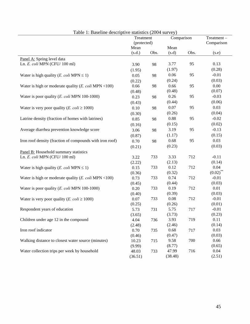
45

Table 1: Baseline descriptive statistics (2004 survey)

Treatment (protected)

Comparison Treatment – Comparison

Mean (s.d.)

Obs.

Mean (s.d)

Obs.

(s.e)

Panel A: Spring level data Ln. E. coli MPN (CFU/ 100 ml) 3.90 98 3.77 95 0.13 (1.95) (1.97) (0.28) Water is high quality (E. coli MPN ≤ 1) 0.05 98 0.06 95 -0.01 (0.22) (0.24) (0.03) Water is high or moderate quality (E. coli MPN <100) 0.66 98 0.66 95 0.00 (0.48) (0.48) (0.07) Water is poor quality (E. coli MPN 100-1000) 0.23 98 0.26 95 -0.03 (0.43) (0.44) (0.06) Water is very poor quality (E. coli ≥ 1000) 0.10 98 0.07 95 0.03 (0.30) (0.26) (0.04) Latrine density (fraction of homes with latrines) 0.85 98 0.88 95 -0.02 (0.16) (0.15) (0.02) Average diarrhea prevention knowledge score 3.06 98 3.19 95 -0.13 (0.87) (1.17) (0.15) Iron roof density (fraction of compounds with iron roof) 0.70 98 0.68 95 0.03 (0.21) (0.23) (0.03) Panel B: Household summary statistics Ln. E. coli MPN (CFU/ 100 ml) 3.22 733 3.33 712 -0.11 (2.22) (2.13) (0.14) Water is high quality (E. coli MPN ≤ 1) 0.15 733 0.12 712 0.04 (0.36) (0.32) (0.02)** Water is high or moderate quality (E. coli MPN <100) 0.73 733 0.74 712 -0.01 (0.45) (0.44) (0.03) Water is poor quality (E. coli MPN 100-1000) 0.20 733 0.19 712 0.01 (0.40) (0.39) (0.03) Water is very poor quality (E. coli ≥ 1000) 0.07 733 0.08 712 -0.01 (0.25) (0.26) (0.01) Respondent years of education 5.73 731 5.75 717 -0.01 (3.65) (3.73) (0.23) Children under age 12 in the compound 4.04 736 3.93 719 0.11 (2.48) (2.46) (0.14) Iron roof indicator 0.70 735 0.68 717 0.03 (0.46) (0.47) (0.03) Walking distance to closest water source (minutes) 10.23 715 9.58 700 0.66 (9.99) (8.77) (0.65) Water collection trips per week by household 48.03 733 47.99 716 0.04 (36.51) (38.48) (2.51)

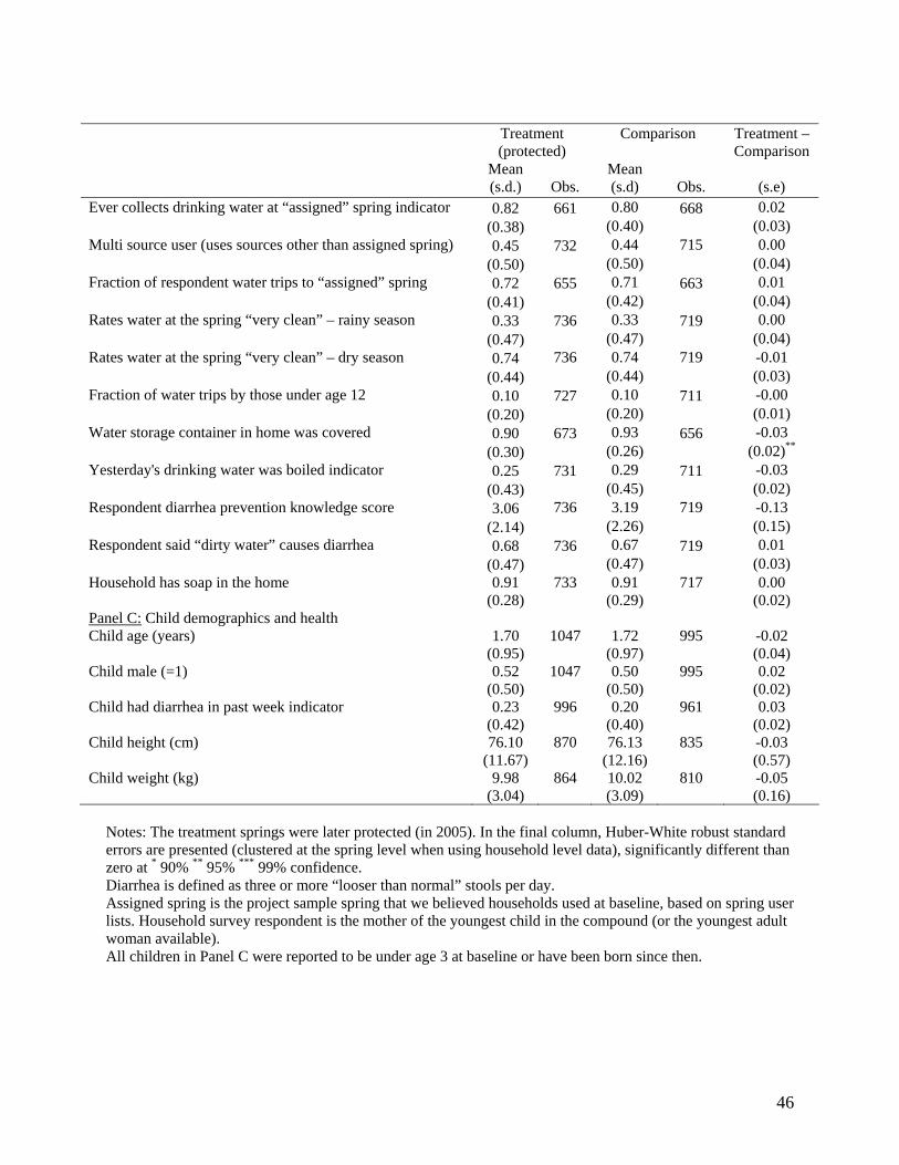
46

Treatment (protected)

Comparison Treatment – Comparison

Mean (s.d.)

Obs.

Mean (s.d)

Obs.

(s.e)

Ever collects drinking water at “assigned” spring indicator 0.82 661 0.80 668 0.02 (0.38) (0.40) (0.03) Multi source user (uses sources other than assigned spring) 0.45 732 0.44 715 0.00 (0.50) (0.50) (0.04) Fraction of respondent water trips to “assigned” spring 0.72 655 0.71 663 0.01 (0.41) (0.42) (0.04) Rates water at the spring “very clean” – rainy season 0.33 736 0.33 719 0.00 (0.47) (0.47) (0.04) Rates water at the spring “very clean” – dry season 0.74 736 0.74 719 -0.01 (0.44) (0.44) (0.03) Fraction of water trips by those under age 12 0.10 727 0.10 711 -0.00 (0.20) (0.20) (0.01) Water storage container in home was covered 0.90 673 0.93 656 -0.03 (0.30) (0.26) (0.02)** Yesterday's drinking water was boiled indicator 0.25 731 0.29 711 -0.03 (0.43) (0.45) (0.02) Respondent diarrhea prevention knowledge score 3.06 736 3.19 719 -0.13 (2.14) (2.26) (0.15) Respondent said “dirty water” causes diarrhea 0.68 736 0.67 719 0.01 (0.47) (0.47) (0.03) Household has soap in the home 0.91 733 0.91 717 0.00 (0.28) (0.29) (0.02) Panel C: Child demographics and health Child age (years) 1.70 1047 1.72 995 -0.02 (0.95) (0.97) (0.04) Child male (=1) 0.52 1047 0.50 995 0.02 (0.50) (0.50) (0.02) Child had diarrhea in past week indicator 0.23 996 0.20 961 0.03 (0.42) (0.40) (0.02) Child height (cm) 76.10 870 76.13 835 -0.03 (11.67) (12.16) (0.57) Child weight (kg) 9.98 864 10.02 810 -0.05 (3.04) (3.09) (0.16)

Notes: The treatment springs were later protected (in 2005). In the final column, Huber-White robust standard errors are presented (clustered at the spring level when using household level data), significantly different than zero at * 90% ** 95% *** 99% confidence. Diarrhea is defined as three or more “looser than normal” stools per day. Assigned spring is the project sample spring that we believed households used at baseline, based on spring user lists. Household survey respondent is the mother of the youngest child in the compound (or the youngest adult woman available). All children in Panel C were reported to be under age 3 at baseline or have been born since then.

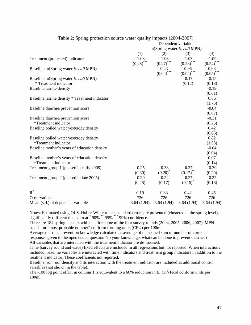
47

Table 2: Spring protection source water quality impacts (2004-2007)

Dependent variable: ln(Spring water E. coli MPN)

(1) (2) (3) (4) Treatment (protected) indicator -1.08 -1.08 -1.03 -1.09 (0.28)*** (0.27)*** (0.23)*** (0.24)*** Baseline ln(Spring water E. coli MPN) 0.43 0.96 0.98 (0.04)*** (0.04)*** (0.05)*** Baseline ln(Spring water E. coli MPN) * Treatment indicator

-0.17 (0.12)

-0.15 (0.13)

Baseline latrine density -0.19 (0.61) Baseline latrine density * Treatment indicator 0.86 (1.75) Baseline diarrhea prevention score -0.04 (0.07) Baseline diarrhea prevention score *Treatment indicator

-0.31 (0.25)

Baseline boiled water yesterday density 0.42 (0.66) Baseline boiled water yesterday density *Treatment indicator

0.82 (1.53)

Baseline mother’s years of education density -0.04 (0.04) Baseline mother’s years of education density *Treatment indicator

0.07 (0.14)

Treatment group 1 (phased in early 2005) -0.25 -0.33 -0.37 -0.30 (0.30) (0.20)* (0.17)** (0.20) Treatment group 2 (phased in late 2005) -0.20 -0.24 -0.27 -0.22 (0.25) (0.17) (0.15)* (0.18) R2 0.19 0.33 0.42 0.45 Observations 726 726 726 726 Mean (s.d.) of dependent variable 3.64 (1.94) 3.64 (1.94) 3.64 (1.94) 3.64 (1.94) Notes: Estimated using OLS. Huber-White robust standard errors are presented (clustered at the spring level), significantly different than zero at * 90% ** 95% *** 99% confidence. There are 184 spring clusters with data for some of the four survey rounds (2004, 2005, 2006, 2007). MPN stands for “most probable number” coliform forming units (CFU) per 100ml. Average diarrhea prevention knowledge calculated as average of demeaned sum of number of correct responses given to the open ended question “to your knowledge, what can be done to prevent diarrhea?” All variables that are interacted with the treatment indicator are de-meaned. Time (survey round and wave) fixed effects are included in all regressions but not reported. When interactions included, baseline variables are interacted with time indicators and treatment group indicators in addition to the treatment indicator. These coefficients not reported. Baseline iron roof density and its interaction with the treatment indicator are included as additional control variables (not shown in the table). The -108 log point effect in column 1 is equivalent to a 66% reduction in E. Coli fecal coliform units per 100ml.

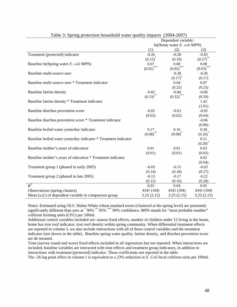
48

Table 3: Spring protection household water quality impacts (2004-2007)

Dependent variable: ln(Home water E. coli MPN)

(1) (2) (3) Treatment (protected) indicator -0.26 -0.28 -0.65 (0.15)* (0.19) (0.27)** Baseline ln(Spring water E. coli MPN) 0.07 0.08 0.08 (0.02)*** (0.02)*** (0.03)*** Baseline multi-source user -0.28 -0.26 (0.17)* (0.17) Baseline multi-source user * Treatment indicator 0.04 0.07 (0.25) (0.25) Baseline latrine density -0.83 -0.84 -0.06 (0.33)** (0.32)*** (0.59) Baseline latrine density * Treatment indicator 1.43 (1.01) Baseline diarrhea prevention score -0.02 -0.03 -0.05 (0.02) (0.02) (0.04) Baseline diarrhea prevention score * Treatment indicator -0.06 (0.06) Baseline boiled water yesterday indicator 0.17 0.16 0.28 (0.08)** (0.08)* (0.16)* Baseline boiled water yesterday indicator * Treatment indicator 0.51 (0.28)* Baseline mother’s years of education 0.01 0.01 0.03 (0.01) (0.01) (0.02) Baseline mother’s years of education * Treatment indicator 0.02 (0.04) Treatment group 1 (phased in early 2005) -0.03 -0.15 -0.03 (0.14) (0.18) (0.27) Treatment group 2 (phased in late 2005) -0.13 -0.17 -0.22 (0.12) (0.16) (0.28) R2 0.03 0.04 0.05 Observations (spring clusters) 4341 (184) 4341 (184) 4341 (184) Mean (s.d.) of dependent variable in comparison group 3.25 (2.15) 3.25 (2.15) 3.25 (2.15)

Notes: Estimated using OLS. Huber-White robust standard errors (clustered at the spring level) are presented, significantly different than zero at * 90% ** 95% *** 99% confidence. MPN stands for “most probable number” coliform forming units (CFU) per 100ml. Additional control variables included are: season fixed effects, number of children under 12 living in the home, home has iron roof indicator, iron roof density within spring community. When differential treatment effects are reported in column 3, we also include interactions with all of these control variables and the treatment indicator (not shown in the table). Baseline spring water quality, latrine density, and diarrhea prevention score are de-meaned. Time (survey round and wave) fixed effects included in all regressions but not reported. When interactions are included, baseline variables are interacted with time effects and treatment group indicators, in addition to interactions with treatment (protected) indicator. These coefficients not reported in the table. The -26 log point effect in column 1 is equivalent to a 23% reduction in E. Coli fecal coliform units per 100ml.

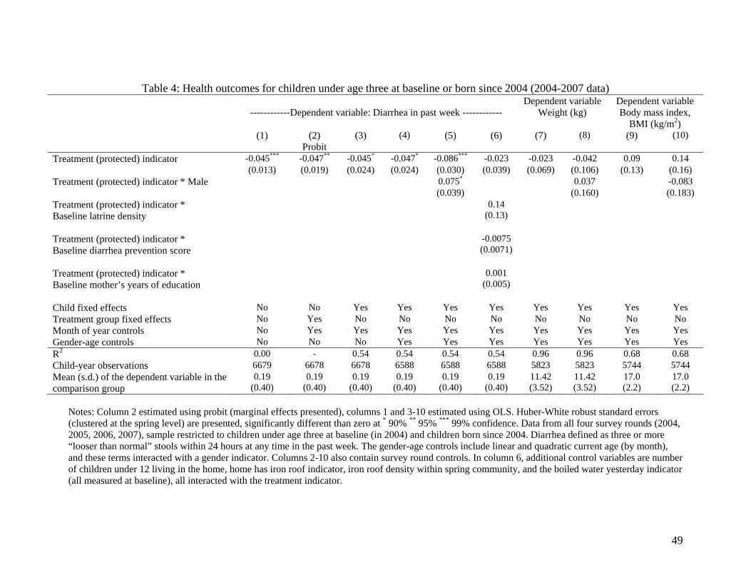
49

Table 4: Health outcomes for children under age three at baseline or born since 2004 (2004-2007 data)

------------Dependent variable: Diarrhea in past week ------------

Dependent variableWeight (kg)

Dependent variable Body mass index,

BMI (kg/m2) (1)

(2)

Probit (3) (4) (5) (6) (7) (8) (9) (10)

Treatment (protected) indicator -0.045*** -0.047** -0.045* -0.047* -0.086*** -0.023 -0.023 -0.042 0.09 0.14 (0.013) (0.019) (0.024) (0.024) (0.030) (0.039) (0.069) (0.106) (0.13) (0.16) Treatment (protected) indicator * Male 0.075* 0.037 -0.083 (0.039) (0.160) (0.183) Treatment (protected) indicator * Baseline latrine density

0.14 (0.13)

Treatment (protected) indicator * Baseline diarrhea prevention score

-0.0075 (0.0071)

Treatment (protected) indicator * Baseline mother’s years of education

0.001 (0.005)

Child fixed effects No No Yes Yes Yes Yes Yes Yes Yes Yes Treatment group fixed effects No Yes No No No No No No No No Month of year controls No Yes Yes Yes Yes Yes Yes Yes Yes Yes Gender-age controls No No No Yes Yes Yes Yes Yes Yes Yes R2 0.00 - 0.54 0.54 0.54 0.54 0.96 0.96 0.68 0.68 Child-year observations 6679 6678 6678 6588 6588 6588 5823 5823 5744 5744 Mean (s.d.) of the dependent variable in the comparison group

0.19 (0.40)

0.19 (0.40)

0.19 (0.40)

0.19 (0.40)

0.19 (0.40)

0.19 (0.40)

11.42 (3.52)

11.42 (3.52)

17.0 (2.2)

17.0 (2.2)

Notes: Column 2 estimated using probit (marginal effects presented), columns 1 and 3-10 estimated using OLS. Huber-White robust standard errors (clustered at the spring level) are presented, significantly different than zero at * 90% ** 95% *** 99% confidence. Data from all four survey rounds (2004, 2005, 2006, 2007), sample restricted to children under age three at baseline (in 2004) and children born since 2004. Diarrhea defined as three or more “looser than normal” stools within 24 hours at any time in the past week. The gender-age controls include linear and quadratic current age (by month), and these terms interacted with a gender indicator. Columns 2-10 also contain survey round controls. In column 6, additional control variables are number of children under 12 living in the home, home has iron roof indicator, iron roof density within spring community, and the boiled water yesterday indicator (all measured at baseline), all interacted with the treatment indicator.

50

Table 5: Treatment effects on household water source choice and health behaviors (2004-2007) Dependent variable

Coefficient (s.e.) on treatment indicator

Full sample

Coefficient (s.e.) on treatment indicator Sole source users

Coefficient (s.e.) on treatment indicator Multi-source users

Mean (s.d.) comparison group in 2006, 2007 surveys

Panel A: Water collection and source choice (1) (2) (3) (4) Use assigned spring for drinking water indicator 0.10 (0.03)*** 0.04 (0.01)*** 0.21 (0.05) *** 0.83 (0.37) Fraction of trips to assigned spring 0.09 (0.03)*** 0.03 (0.02)* 0.20 (0.05) *** 0.76 (0.40) Perceive water at assigned spring to be very clean – rainy season 0.18 (0.03) *** 0.17 (0.04) *** 0.18 (0.04) *** 0.12 (0.33) Perceive water at assigned spring to be very clean – dry season 0.09 (0.03) *** 0.05 (0.03)* 0.13 (0.05) *** 0.51 (0.50) Self-reported distance to nearest water (min.) -1.41 (0.44) *** -1.71 (0.48) *** -1.03 (0.80) 7.92 (7.23) Calculated distance (GPS) to assigned spring (km) 0.03 (0.03) 0.06 (0.05) 0.01 (0.01) 0.36 (2.52) Trips made to get water (all uses, members, sources) past week -2.46 (2.15) -0.86 (2.39) -4.52 (3.51) 31.77 (24.42)

Panel B: Water transportation and storage Fraction of water trips by those under age 12(a) 0.00 (0.01) 0.00 (0.02) -0.00 (0.02) 0.09 (0.19) Water storage container in home covered indicator 0.00 (0.01) -0.01 (0.02) 0.01 (0.02) 0.98 (0.15) Ever treated water with chlorine indicator(b) 0.03 (0.03) 0.04 (0.05) 0.02 (0.05) 0.45 (0.50) Yesterday’s drinking water boiled indicator(c) 0.04 (0.02) 0.05 (0.03)* 0.01 (0.03) 0.25 (0.44)

Panel C: Sanitation and hygiene behaviors Diarrhea prevention knowledge score 0.10 (0.13) 0.19 (0.16) -0.01 (0.17) 2.65 (2.50) Respondent says drinking clean water is a way to prevent diarrhea -0.03 (0.02) -0.03 (0.03) -0.03 (0.04) 0.50 (0.50) Household has soap in the home indicator -0.01 (0.02) -0.01 (0.02) 0.01 (0.03) 0.89 (0.31) Fingers with bacterial contamination (Enterococcus colonies) 0.09 (0.13) 0.08 (0.17) 0.26 (0.24) 0.71 (1.26)

Panel D: Spring amenities (recorded by enumerators) (d) Spring has “clear” water 0.26 (0.07) *** - - 0.71 (0.45) Fence around spring 0.95 (0.03) *** - - 0.00 (0.00) Spring has “high” water yield -0.05 (0.06) - - 0.73 (0.45) Fecal matter around spring -0.15 (0.06) ** - - 0.27 (0.44) Animals around spring -0.03 (0.06) - - 0.12 (0.33) Trench for spring water cleared in last month 0.29 (0.11) *** - - 0.59 (0.49) Vegetation near spring cleared in last month 0.17 (0.10) * - - 0.36 (0.48) Reported spring maintenance quality (5=excellent, 1=poor) -0.53 (0.14) *** - - 3.21 (0.92)

51

Notes: N=1354 households at 184 springs (full sample), 755 of whom are baseline sole source users. Each cell reports the differences-in-differences treatment effect estimate from a separate regression, where the dependent variable is reported in the first column. Huber-White robust standard errors (clustered at the spring level) are presented, significantly different than zero at * 90% ** 95% *** 99% confidence. Reported means of the dependent variables are in the comparison group 2006 and 2007 (rounds 2 & 3 post-treatment) surveys. Assigned spring is the project sample spring that we believed households used at baseline based on spring user lists. The fingertip contamination results are for the respondent’s main hand (so values range from 0-5). (a): Because of changes in survey design, responses to this question are not available for the third (2006) round of data collection. (b): Because of changes in survey design, responses to this question are not available for the first (2004) round of data collection. (c): Because of changes in survey design, responses to this question are not available for the fourth (2007) round of data collection. (d): Panel D contains spring level information, so the breakdown into sole source and multi-source households is not possible.

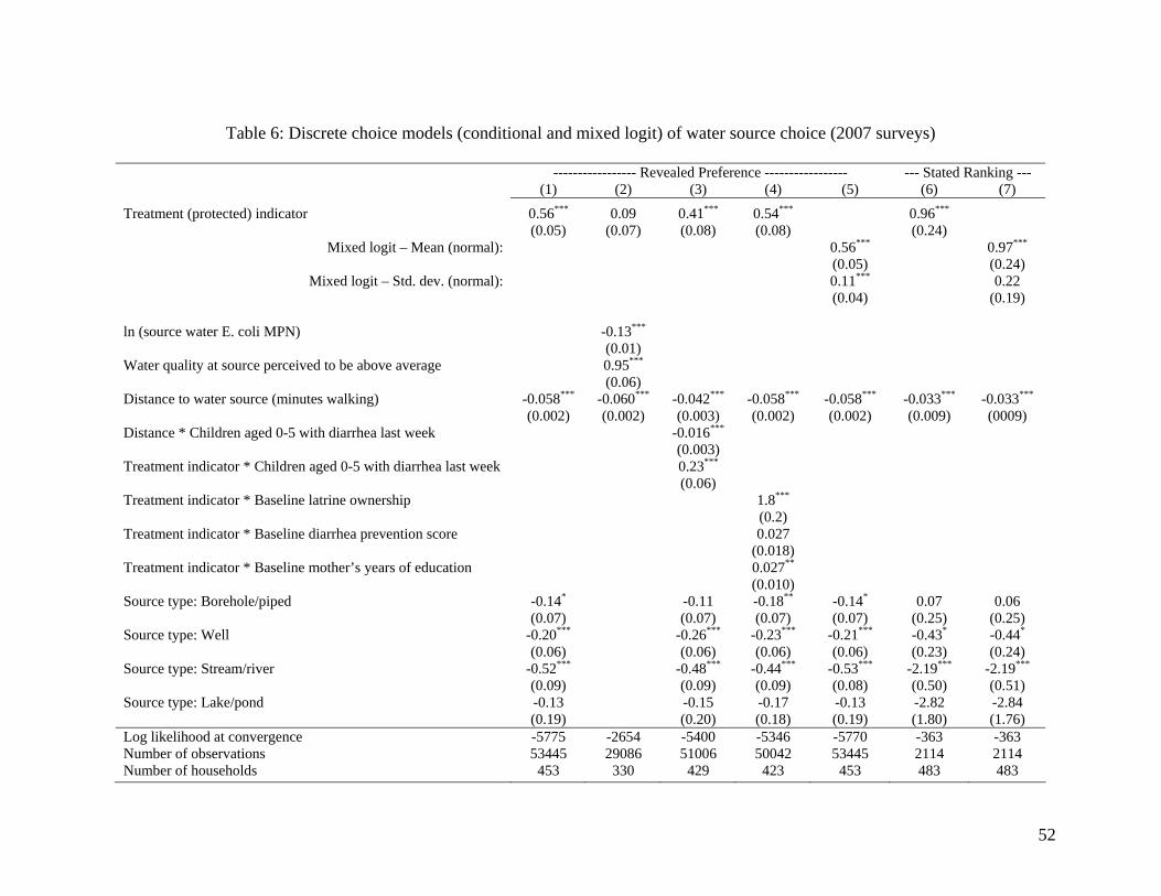
52

Table 6: Discrete choice models (conditional and mixed logit) of water source choice (2007 surveys)

----------------- Revealed Preference ----------------- --- Stated Ranking --- (1) (2) (3) (4) (5) (6) (7)

Treatment (protected) indicator 0.56*** 0.09 0.41*** 0.54*** 0.96*** (0.05) (0.07) (0.08) (0.08) (0.24)

Mixed logit – Mean (normal):

0.56*** (0.05)

0.97*** (0.24)

Mixed logit – Std. dev. (normal):

0.11*** (0.04)

0.22 (0.19)

ln (source water E. coli MPN) -0.13*** (0.01) Water quality at source perceived to be above average 0.95*** (0.06) Distance to water source (minutes walking) -0.058*** -0.060*** -0.042*** -0.058*** -0.058*** -0.033*** -0.033*** (0.002) (0.002) (0.003) (0.002) (0.002) (0.009) (0009) Distance * Children aged 0-5 with diarrhea last week -0.016*** (0.003) Treatment indicator * Children aged 0-5 with diarrhea last week 0.23*** (0.06) Treatment indicator * Baseline latrine ownership 1.8*** (0.2) Treatment indicator * Baseline diarrhea prevention score 0.027 (0.018) Treatment indicator * Baseline mother’s years of education 0.027** (0.010) Source type: Borehole/piped -0.14* -0.11 -0.18** -0.14* 0.07 0.06 (0.07) (0.07) (0.07) (0.07) (0.25) (0.25) Source type: Well -0.20*** -0.26*** -0.23*** -0.21*** -0.43* -0.44* (0.06) (0.06) (0.06) (0.06) (0.23) (0.24) Source type: Stream/river -0.52*** -0.48*** -0.44*** -0.53*** -2.19*** -2.19*** (0.09) (0.09) (0.09) (0.08) (0.50) (0.51) Source type: Lake/pond -0.13 -0.15 -0.17 -0.13 -2.82 -2.84 (0.19) (0.20) (0.18) (0.19) (1.80) (1.76) Log likelihood at convergence -5775 -2654 -5400 -5346 -5770 -363 -363 Number of observations 53445 29086 51006 50042 53445 2114 2114 Number of households 453 330 429 423 453 483 483

53

Notes: Conditional logit model in columns 1-4 and 6 and mixed logit model in columns 5 and 7 (grouped by trip or choice situation, and weighting each household equally). Significantly different than zero at * 90 ** 95 *** 99% confidence. In columns 1-5 each observation represents a unique household-water source pair in a given water collection trip. In columns 6-7, each observation represents a household-water source pair from a series of questions in which the respondent is asked to choose their favorite source from among alternatives. The data are from the final round of household surveys (2007). The dependent variable is an indicator equaling 1 if the household chose the source represented in that household-water source pair in that collection trip. The omitted water source category is “non-program spring”. The coefficient estimate on the indicator for being the assigned program sample spring, the spring that we believe households used at baseline based on spring user lists, is not shown. In column 3, additional controls are included for children aged 0-5 and 5-12 at baseline, and the distance to water source term, directly and interacted with the treatment indicator (not shown). In column 4, additional control variables are number of children under 12 living in the home, home has iron roof indicator, iron roof density within spring community, and the boiled water yesterday indicator (all measured at baseline), directly and interacted with the treatment indicator.

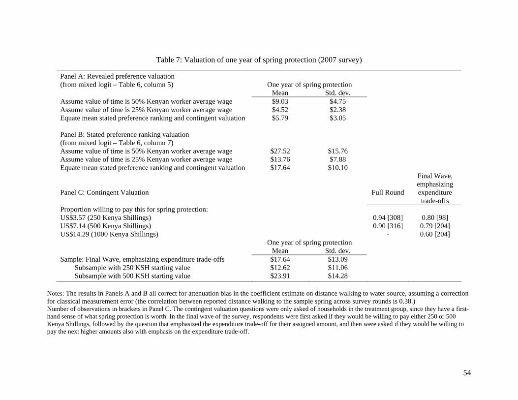
54

Table 7: Valuation of one year of spring protection (2007 survey)

Panel A: Revealed preference valuation (from mixed logit – Table 6, column 5)

One year of spring protection

Mean Std. dev. Assume value of time is 50% Kenyan worker average wage $9.03 $4.75 Assume value of time is 25% Kenyan worker average wage $4.52 $2.38 Equate mean stated preference ranking and contingent valuation $5.79 $3.05 Panel B: Stated preference ranking valuation (from mixed logit – Table 6, column 7)

Assume value of time is 50% Kenyan worker average wage $27.52 $15.76 Assume value of time is 25% Kenyan worker average wage $13.76 $7.88 Equate mean stated preference ranking and contingent valuation $17.64 $10.10 Panel C: Contingent Valuation

Full Round

Final Wave, emphasizing expenditure trade-offs

Proportion willing to pay this for spring protection: US$3.57 (250 Kenya Shillings) 0.94 [308] 0.80 [98] US$7.14 (500 Kenya Shillings) 0.90 [316] 0.79 [204] US$14.29 (1000 Kenya Shillings) - 0.60 [204] One year of spring protection Mean Std. dev. Sample: Final Wave, emphasizing expenditure trade-offs $17.64 $13.09 Subsample with 250 KSH starting value $12.62 $11.06 Subsample with 500 KSH starting value $23.91 $14.28

Notes: The results in Panels A and B all correct for attenuation bias in the coefficient estimate on distance walking to water source, assuming a correction for classical measurement error (the correlation between reported distance walking to the sample spring across survey rounds is 0.38.) Number of observations in brackets in Panel C. The contingent valuation questions were only asked of households in the treatment group, since they have a first-hand sense of what spring protection is worth. In the final wave of the survey, respondents were first asked if they would be willing to pay either 250 or 500 Kenya Shillings, followed by the question that emphasized the expenditure trade-off for their assigned amount, and then were asked if they would be willing to pay the next higher amounts also with emphasis on the expenditure trade-off.

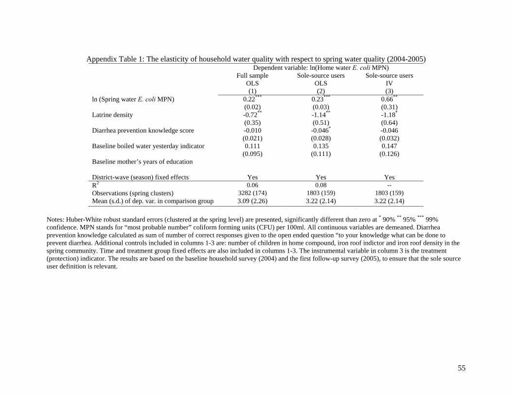
55

Appendix Table 1: The elasticity of household water quality with respect to spring water quality (2004-2005)

Dependent variable: ln(Home water E. coli MPN) Full sample

OLS Sole-source users

OLS Sole-source users

IV (1) (2) (3) ln (Spring water E. coli MPN) 0.22*** 0.23*** 0.66** (0.02) (0.03) (0.31) Latrine density -0.72** -1.14** -1.18* (0.35) (0.51) (0.64) Diarrhea prevention knowledge score -0.010 -0.046* -0.046 (0.021) (0.028) (0.032) Baseline boiled water yesterday indicator 0.111 0.135 0.147 (0.095) (0.111) (0.126) Baseline mother’s years of education District-wave (season) fixed effects Yes Yes Yes R2 0.06 0.08 -- Observations (spring clusters) 3282 (174) 1803 (159) 1803 (159) Mean (s.d.) of dep. var. in comparison group 3.09 (2.26) 3.22 (2.14) 3.22 (2.14)

Notes: Huber-White robust standard errors (clustered at the spring level) are presented, significantly different than zero at * 90% ** 95% *** 99% confidence. MPN stands for “most probable number” coliform forming units (CFU) per 100ml. All continuous variables are demeaned. Diarrhea prevention knowledge calculated as sum of number of correct responses given to the open ended question “to your knowledge what can be done to prevent diarrhea. Additional controls included in columns 1-3 are: number of children in home compound, iron roof indictor and iron roof density in the spring community. Time and treatment group fixed effects are also included in columns 1-3. The instrumental variable in column 3 is the treatment (protection) indicator. The results are based on the baseline household survey (2004) and the first follow-up survey (2005), to ensure that the sole source user definition is relevant.

56

Figure 1: Rural Water Project (RWP) study region and sample springs

57

Figure 2: Rural Water Project (RWP) Timeline 2004-2007

Household surveys, water testing; April-August 2005 (Nsprings=175, Nhh=1,250)

Identified universe of springs; June-July 2004 (Nsprings=562)

Conducted initial site visits and water quality tests, Further site visits with Ministry of Water and NGO technical staff, Selection of sample; July-November 2004 (Nsprings=200)

Spring user lists compiled; July 2004-January 2005 (Nsprings=200)

Randomization of springs into year of treatment (Nsprings=200) Random selection of 7-8 households per spring (Nhh=1500)

Household baseline surveys, water quality testing; August 2004-February 2005 (Nsprings= 184, Nhh=1384 in viable sample)

Year 1 spring protection; January-April 2005 (Nsprings=47)

Year 1 Treatment (Nsprings=50; Nhh=371) Sample after nonviable springs eliminated (Nsprings=47; Nhh=350)

Years 3 and 4 Treatment (Nsprings=100; Nhh=751) Sample after nonviable springs eliminated (Nsprings=91; Nhh=685)

Year 2 Treatment (Nsprings=50; Nhh=378) Sample after nonviable springs eliminated (Nsprings=46; Nhh=349)

Year 2 spring protection; August-November 2005 (Nsprings=46)

Household surveys, water testing; August-November 2006 (Nsprings=183, Nhh=1,283) Household surveys, water testing; January-March 2007 (Nsprings=184, Nhh=1,231)

58

Figure 3: Change in spring water contamination from 2004 to 2007 versus baseline (2004) water contamination

-4-2

02

Cha

nge

in S

prin

g ln

E C

oli M

PN20

04 to

200

7

0 2 4 6 8Baseline Spring ln E Coli MPN

Treatment Groups 1 and 2 Comparison Group

Notes: To 10-90 range in Baseline ln (E Coli MPN) is [1.1, 6.3]. MPN stands for “most probable number” coliform forming units (CFU) per 100ml.

59

Figure 4: Household revealed preference and stated preference valuations of one year of spring protection (2007)

$5.79 $17.64

0.1

.2.3

.4N

orm

al d

istri

butio

n de

nsity

-20 0 20 40 60

Revealed preference (US$) Stated ranking (US$)Contingent Valuation (US$)

Notes: The revealed preference estimates are from the mixed logit results in Table 6, regression 5, and the stated preference ranking results are from the mixed.logit results in Table 6, regression 7. The contingent valuation data are presented in Table 7, Panel C.