Spreadsheets in Finance and Forecasting Presentation 8: Problem Solving

Spreadsheets in Finance and Forecasting

Presentation 8: Problem Solving

Objectives After studying the materials for

week 8, you will be able to: Set up “what-if” scenarios and

summaries Use goal-seek to find the solution to

specific problems Use solver to find the solution to more

general problems

Working Methods You should work through each section of this

presentation either in groups, or individually, taking notes.

Read through the details of each section carefully, then when you come to the blue “Action point” sticker, carry out the tasks that you are asked to do.

If you have difficulties, go back and re-read the section

Only move on to the next section when you have completed the task successfully

Presentation Sections

Click on the button to view the section

Introduction

Scenarios

Goal Seeking

Solver

Introduction

Problem Solving Excel provides many features to help

managers solve problems and to make decisions.These include: Creating Scenarios: Using “What if?”

situations to look at several different options

Goal Seeking: Finding a value of a particular variable to meet specific conditions

Solver: Finding solutions to complex problems by imposing sets of conditions on groups of cells.

Problem Solving During this lecture,

we will look at each one of these in turn.

In order to help you understand each of these features, we will look at one situation:

Loan Payment

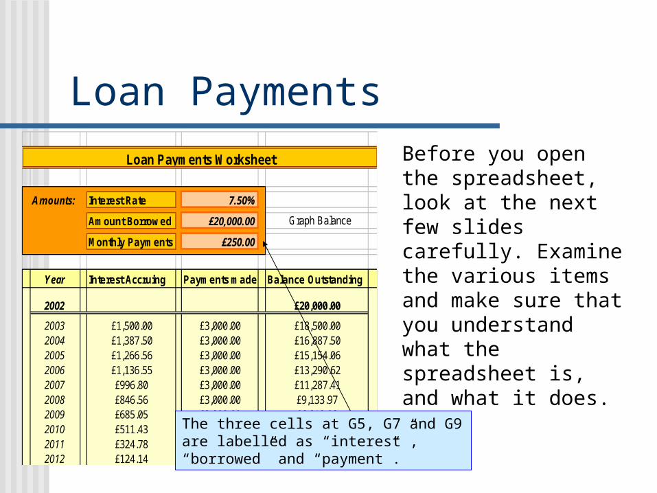
Loan Payments

Amounts: Interest Rate 7.50%

Amount Borrowed £20,000.00

Monthly Payments £250.00

Year Interest Accruing Payments made Balance Outstanding

2002 £20,000.00

2003 £1,500.00 £3,000.00 £18,500.002004 £1,387.50 £3,000.00 £16,887.502005 £1,266.56 £3,000.00 £15,154.062006 £1,136.55 £3,000.00 £13,290.622007 £996.80 £3,000.00 £11,287.412008 £846.56 £3,000.00 £9,133.972009 £685.05 £3,000.00 £6,819.022010 £511.43 £3,000.00 £4,330.442011 £324.78 £3,000.00 £1,655.232012 £124.14 £3,000.00 -£1,220.63

Loan Payments Worksheet

Graph Balance

Before you open the spreadsheet, look at the next few slides carefully. Examine the various items and make sure that you understand what the spreadsheet is, and what it does.

The three cells at G5, G7 and G9 are labelled as “interest”, “borrowed” and “payment”.

Loan Payments





2002 £20,000.00

2003 £1,500.00 £3,000.00 £18,500.002004 £1,387.50 £3,000.00 £16,887.502005 £1,266.56 £3,000.00 £15,154.062006 £1,136.55 £3,000.00 £13,290.622007 £996.80 £3,000.00 £11,287.412008 £846.56 £3,000.00 £9,133.972009 £685.05 £3,000.00 £6,819.022010 £511.43 £3,000.00 £4,330.442011 £324.78 £3,000.00 £1,655.232012 £124.14 £3,000.00 -£1,220.63


Graph Balance

This shows the following situation : The interest rate is

7.5% per annum We borrowed

£20000 Payments are £250

per month The loan was taken

out in 2002 The loan will be

paid off some time during 2012.

The negative amount means that if the payments continue, the amount owing would be negative, i.e. the lender would owe you money!

Loan Payments

Note that the final amount runs into the negative region.





2002 £30,000.00

2003 £1,950.00 £4,800.00 £27,150.002004 £1,764.75 £4,800.00 £24,114.752005 £1,567.46 £4,800.00 £20,882.212006 £1,357.34 £4,800.00 £17,439.552007 £1,133.57 £4,800.00 £13,773.122008 £895.25 £4,800.00 £9,868.382009 £641.44 £4,800.00 £5,709.822010 £371.14 £4,800.00 £1,280.962011 £83.26 £4,800.00 -£3,435.782012 -£223.33 £4,800.00 -£8,459.102013 -£549.84 £4,800.00 -£13,808.952014 -£897.58 £4,800.00 -£19,506.532015 -£1,267.92 £4,800.00 -£25,574.45


Graph Balance

Loan Repayment

-£10,000.00

£0.00

£10,000.00

£20,000.00

£30,000.00

£40,000.00

2002

2003

2004

2005

2006

2007

2008

2009

2010

2011

Pressing the “Graph Balance” button runs a macro which shows a chart illustrating the level of the balance outstanding at the end of each year.

Activity You should now open

up the Loan Payments spreadsheet.

Experiment with the amounts in the cells G5, G7 & G9, and with the Graph

Ensure that you fully understand what the spreadsheet is doing before you carry on.

Action Point !

Return to Menu

Scenarios

Scenarios Your small business is doing

well You decide to expand, and

ask the bank for a loan. You need at least £30 000,

and the bank offers you up to £50 000.

The bank will charge you 6.5% interest

You can only afford £400 per month. Is this sufficient to pay off the loan?

Scenario 1 Let’s start with the

smallest amount needed, £30 000

The bank will charge you interest of 6.5%

Set your monthly payments to £400.

Is this sufficient to pay off the loan?

Scenario 1 The amount is

£30 000 The interest is

6.5% Monthly

payments are £400.

Enter the details into the correct boxes in the Loan Payments Spreadsheet

Action Point !

Now, Can we pay off the

loan?

Scenario 1 You should have entered these

amounts into the boxes.




So, when will the loan be paid

off?

Scenario 1

The amount outstanding is: £1280.96

(positive) in 2010, £3435.78

(negative) in 2011 This means that

the loan would be paid off some time during 2011


2002 £30,000.00

2003 £1,950.00 £4,800.00 £27,150.002004 £1,764.75 £4,800.00 £24,114.752005 £1,567.46 £4,800.00 £20,882.212006 £1,357.34 £4,800.00 £17,439.552007 £1,133.57 £4,800.00 £13,773.122008 £895.25 £4,800.00 £9,868.382009 £641.44 £4,800.00 £5,709.822010 £371.14 £4,800.00 £1,280.962011 £83.26 £4,800.00 -£3,435.782012 -£223.33 £4,800.00 -£8,459.10

Saving a Scenario This is the first of our “what if?”

scenarios. Excel allows us to store these

scenarios for future reference, and compare them one with another.

Over the next few slides, this method will be explained.

Creating a Scenario Click on Tools , then

Scenarios, then Add In Scenario Name, put

“Small Amount” Then click here; Now click on cell G7 Click OK Click OK again on the

next box Then Close on the last

box

Action Point !

What exactly is a Scenario? A scenario simply

is a description of a particular situation, defined by particular values of certain variables

Excel stores these Scenarios, and you can return to them

Scenario 2 Let’s move on to the a

larger amount. Suppose we borrow £40 000

The bank will still charge you interest of 6.5%

The monthly payments are still £400.

Is this sufficient to pay off the loan?

Action Point !

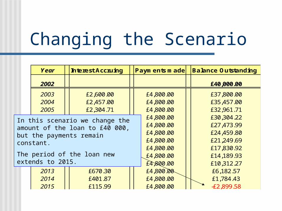
Changing the Scenario


2002 £40,000.00

2003 £2,600.00 £4,800.00 £37,800.002004 £2,457.00 £4,800.00 £35,457.002005 £2,304.71 £4,800.00 £32,961.712006 £2,142.51 £4,800.00 £30,304.222007 £1,969.77 £4,800.00 £27,473.992008 £1,785.81 £4,800.00 £24,459.802009 £1,589.89 £4,800.00 £21,249.692010 £1,381.23 £4,800.00 £17,830.922011 £1,159.01 £4,800.00 £14,189.932012 £922.35 £4,800.00 £10,312.272013 £670.30 £4,800.00 £6,182.572014 £401.87 £4,800.00 £1,784.432015 £115.99 £4,800.00 -£2,899.58

In this scenario we change the amount of the loan to £40 000, but the payments remain constant.

The period of the loan new extends to 2015.

Changing the Scenario


2002 £40,000.00

2003 £2,600.00 £4,800.00 £37,800.002004 £2,457.00 £4,800.00 £35,457.002005 £2,304.71 £4,800.00 £32,961.712006 £2,142.51 £4,800.00 £30,304.222007 £1,969.77 £4,800.00 £27,473.992008 £1,785.81 £4,800.00 £24,459.802009 £1,589.89 £4,800.00 £21,249.692010 £1,381.23 £4,800.00 £17,830.922011 £1,159.01 £4,800.00 £14,189.932012 £922.35 £4,800.00 £10,312.272013 £670.30 £4,800.00 £6,182.572014 £401.87 £4,800.00 £1,784.432015 £115.99 £4,800.00 -£2,899.58

Create a New Scenario, and call it “Medium Amount”

Action Point !

Final Scenario Change the amount of

the loan to £50 000 Store this Scenario as

“Large Amount”

Action Point !

Comparing Scenarios We can re-examine

the scenarios once we have stored them by clicking on Tools - Scenarios, and then selecting the particular Scenario:

Small, Medium or Large Amounts

Then click OK. When will the loan be paid off in each case?

Deleting Scenarios Select Tools-

Scenario Delete Each of

the three Scenarios in turn.

Action Point !

Scenario Challenge Now Create three different

scenarios, in which the Loan is £40000, and the payments are £450 per month In scenario A

(low interest) the interest is 4%

In scenario B(medium interest) the interest is 7%

In scenario C(high interest) the interest is 10%

What amount of the loan is remaining in 2010 in each case?

Action Point !

Scenario Challenge In scenario A (low interest) £4,985.94 is left in 2010

In scenario B (medium interest) £13,324.51 is left in 2010

In scenario C (high interest)£23,989.76 is left in 2010

Scenario Summaries

Click on Tools – Scenario and Summary

Select Scenario Summary use as “results cell” the amount owing in 2010 (Cell I22)

Click OKAction Point !

Scenario Summary

This is the Summary Page. The values in cell I22 can now be compared

across the three scenarios.

Scenario SummaryCurrent Values: High Interest Medium Interest Low Interest

Changing Cells:interest 10.00% 10.00% 7.00% 4.00%

Result Cells:$I$22 £23,989.76 £23,989.76 £13,324.51 £4,985.94

Notes: Current Values column represents values of changing cells attime Scenario Summary Report was created. Changing cells for eachscenario are highlighted in gray.

Follow-up Activities You should now

examine the first section of Formative Activity 8.

This challenges you to find a range solutions to particular problems for a Software-producing company

Return to Menu

Goal Seeking

Goal Seeking In Goal Seeking,

we look at specific Scenarios in which particular cells achieve target values.

These are achieved by altering other, named cells.

Goal Seeking For example:

Suppose we wish to borrow £50,000.

The interest rate is fixed at 6.5%, but we would like to pay this back by 2010 at the latest.

To do this will mean changing the monthly payments.




Goal Seeking Click on Tools – Goal

Seek We set cell I22 to

zero. (This is the amount owing in 2010)

We will make changes to cell G9; this is the value representing the monthly payments.Action

Point !

Goal Seeking - Solution This box shows

that a solution has been found.

OK, so where is the solution to the problem?

Goal Seeking Solutions In this solution, we borrow £50 000, at 6.5%, and pay the

loan back by the end of 2010. In order to achieve this, we changed cell G9. This shows

that the payments need to be £684.32Amounts: Interest Rate 6.50%




2002 £50,000.00

2003 £3,250.00 £8,211.86 £45,038.142004 £2,927.48 £8,211.86 £39,753.752005 £2,583.99 £8,211.86 £34,125.882006 £2,218.18 £8,211.86 £28,132.202007 £1,828.59 £8,211.86 £21,748.922008 £1,413.68 £8,211.86 £14,950.742009 £971.80 £8,211.86 £7,710.672010 £501.19 £8,211.86 £0.00

Graph Balance

Challenge Suppose we borrow

money at 4.5% interest and we need to pay back the loan by the end of 2012.

We can afford to pay £550 per month .

What is the maximum amount of the loan we can afford?

Action Point !

Solution





2002 £52,223.94

2003 £2,350.08 £6,600.00 £47,974.022004 £2,158.83 £6,600.00 £43,532.852005 £1,958.98 £6,600.00 £38,891.832006 £1,750.13 £6,600.00 £34,041.962007 £1,531.89 £6,600.00 £28,973.852008 £1,303.82 £6,600.00 £23,677.672009 £1,065.50 £6,600.00 £18,143.162010 £816.44 £6,600.00 £12,359.612011 £556.18 £6,600.00 £6,315.792012 £284.21 £6,600.00 £0.00

Graph Balance

The Goal Seeker has converged on the amount of £52, 223.94

This is paid off by the end of 2012

Here you needed to set cell I22 to zero

by changing cell G7

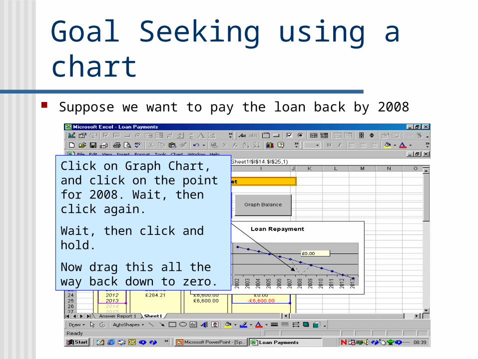
Goal Seeking using a chart

Click on Graph Chart, and click on the point for 2008. Wait, then click again.

Wait, then click and hold.

Now drag this all the way back down to zero.

Suppose we want to pay the loan back by 2008

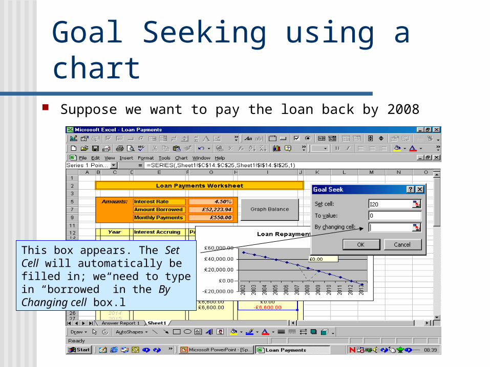
Goal Seeking using a chart Suppose we want to pay the loan back by 2008

This box appears. The Set Cell will automatically be filled in; we need to type in “borrowed” in the By Changing cell box.l

The Solution found!

This shows the new data using the original chart parameters; this means that if you had kept on paying in the same way for the same amount of time, then the loan company would be in debt to you.


examine the second section of Formative Activity 8.

This section uses Goal Seeking to work out the Break-Even Price for products retailed by the software-producing company

Return to Menu

Solver

Solver Solver is an “Add-

in” which extends the idea of goal-seeking.

Instead of changing one cell, solver changes a number of cells to meet a target criterion.

The First Step If your Tools menu

does not have “Solver”, you need to select “Add-Ins” and select “Solver Add-in”

The Solver will then be part of the Tools menu.

The Problem We wish to borrow

up to £50 000 We can afford up

to £600 per month The interest will be

at least 4% We wish to pay off

the loan at the latest by the end of 2018

Solver parameters You need to add in

the parameters of the cells which will change: borrowed, interest, payment (cells G5, G7 and G9)

In addition you need to specify the cell value which you need to converge on: in this case, I30, which we will set at Zero.

Action Point !

Solving the problem We set cell G7 – “borrowed” at less than 50000; We set cell G5 – “interest” at – at least 4% (0.04) We set cell G9 – “payments” at less than £600 The target cell I30, the amount owing in 2018, is set to zero.

Use the Add button to add in these constraints

Solver Results

This box appears when a solution has been found. The options allow you to change he values of the variables

to the current solution, or to save it as a scenario. We can also get reports on the Answer, and how close Excel

was in finding a solution to the given constraints.

Have we found a solution?4





2002 £20,003.27

2003 £800.13 £1,716.68 £19,086.722004 £763.47 £1,716.68 £18,133.512005 £725.34 £1,716.68 £17,142.172006 £685.69 £1,716.68 £16,111.172007 £644.45 £1,716.68 £15,038.942008 £601.56 £1,716.68 £13,923.822009 £556.95 £1,716.68 £12,764.092010 £510.56 £1,716.68 £11,557.972011 £462.32 £1,716.68 £10,303.612012 £412.14 £1,716.68 £8,999.072013 £359.96 £1,716.68 £7,642.362014 £305.69 £1,716.68 £6,231.372015 £249.25 £1,716.68 £4,763.942016 £190.56 £1,716.68 £3,237.822017 £129.51 £1,716.68 £1,650.652018 £66.03 £1,716.68 £0.002019 £0.00 £1,716.68 -£1,716.682020 -£68.67 £1,716.68 -£3,502.03

Graph Balance

It is certainly true that:

“borrowed” is less than 50000;

“interest” is at least 4% (0.04)

“payments” is less than £600

the amount owing in 2018, is set to zero

Is this what we wanted?4





2002 £20,003.27

2003 £800.13 £1,716.68 £19,086.722004 £763.47 £1,716.68 £18,133.512005 £725.34 £1,716.68 £17,142.172006 £685.69 £1,716.68 £16,111.172007 £644.45 £1,716.68 £15,038.942008 £601.56 £1,716.68 £13,923.822009 £556.95 £1,716.68 £12,764.092010 £510.56 £1,716.68 £11,557.972011 £462.32 £1,716.68 £10,303.612012 £412.14 £1,716.68 £8,999.072013 £359.96 £1,716.68 £7,642.362014 £305.69 £1,716.68 £6,231.372015 £249.25 £1,716.68 £4,763.942016 £190.56 £1,716.68 £3,237.822017 £129.51 £1,716.68 £1,650.652018 £66.03 £1,716.68 £0.002019 £0.00 £1,716.68 -£1,716.682020 -£68.67 £1,716.68 -£3,502.03

Graph Balance

Not really.

The question should have been:

“What is the maximum amount we can borrow at 4%, if we are prepared to pay £600 per month, but want to pay the money off in 2018?”

The solver dialogue box

The question should have been:

“What is the maximum amount we can borrow at 4%, if we are prepared to pay up to £600 per month, but want to pay the money off in 2018?”

Here we need to change the amount borrowed to a minimum amount; this will force solver to give us a solution.

Use the Change button, to modify the Constraints

Three Scenarios4




4Amounts: Interest Rate 4.00%






The three scenarios all are feasible solutions

However if we want force solver to find the maximum we can borrow, we should set the payment to 600

Another Feasible Solution





2002 £60,000.00

2003 £5,375.74 £7,200.00 £58,175.742004 £5,212.30 £7,200.00 £56,188.042005 £5,034.21 £7,200.00 £54,022.242006 £4,840.16 £7,200.00 £51,662.402007 £4,628.73 £7,200.00 £49,091.132008 £4,398.35 £7,200.00 £46,289.482009 £4,147.34 £7,200.00 £43,236.822010 £3,873.83 £7,200.00 £39,910.652011 £3,575.82 £7,200.00 £36,286.472012 £3,251.11 £7,200.00 £32,337.592013 £2,897.31 £7,200.00 £28,034.892014 £2,511.81 £7,200.00 £23,346.702015 £2,091.76 £7,200.00 £18,238.462016 £1,634.09 £7,200.00 £12,672.552017 £1,135.41 £7,200.00 £6,607.962018 £592.04 £7,200.00 £0.00


Graph Balance

Here solver tells us that for payments of £600 per month, we can support a loan of £60 000 and pay it off by 2018, even if the interest rate were to rise to 8.96%

However, what is the maximum loan we can take out at 4%, and still pay it

off by the deadline?

The Solution





2002 £83,896.53

2003 £3,355.86 £7,200.00 £80,052.392004 £3,202.10 £7,200.00 £76,054.492005 £3,042.18 £7,200.00 £71,896.662006 £2,875.87 £7,200.00 £67,572.532007 £2,702.90 £7,200.00 £63,075.432008 £2,523.02 £7,200.00 £58,398.452009 £2,335.94 £7,200.00 £53,534.392010 £2,141.38 £7,200.00 £48,475.762011 £1,939.03 £7,200.00 £43,214.792012 £1,728.59 £7,200.00 £37,743.392013 £1,509.74 £7,200.00 £32,053.122014 £1,282.12 £7,200.00 £26,135.252015 £1,045.41 £7,200.00 £19,980.662016 £799.23 £7,200.00 £13,579.882017 £543.20 £7,200.00 £6,923.082018 £276.92 £7,200.00 £0.00


Graph Balance

Here solver tells us that for payments of £600 per month, we can support a loan of £83 896.53 and pay it off by 2018, provided that the interest rate does not rise higher than 4%

In fact, we could have found this using Goal Seek!

Working with the Tools As you have seen, these

spreadsheet tools are quite sophisticated, and therefore require you to ask the right questions in the right manner, before they supply you with the solution to your problem.

Asking the wrong question will still lead you to a correct answer – but not to the problem you are trying to solve!


examine the final three sections of Formative Activity 8.

This challenges you to use Solver find a range of solutions to particular problems for the software-producing company

Return to Menu

Documents

Spreadsheets in Finance and Forecasting Presentation 8: Problem Solving