Spread balanced Wannier functions: Robust and automatable orbital localization

Pietro F. Fontana, Ask H. Larsen, Thomas Olsen, and Kristian S. Thygesen∗CAMD, Department of Physics, Technical University of Denmark, DK-2800 Kongens Lyngby, Denmark

(Dated: November 9, 2021)

We introduce a new type of Wannier functions (WFs) obtained by minimizing the conventionalspread functional with a penalty term proportional to the variance of the spread distribution. Thismodified Wannierisation scheme is less prone to produce ineffective solutions featuring one or severalpoorly localized orbitals, making it well suited for complex systems or high-throughput applications.Furthermore, we propose an automatable protocol for selecting the initial guess and determine theoptimal number of bands (or equivalently WFs) for the localization algorithm. The improved per-formance and robustness of the approach is demonstrated for a diverse set of test systems includingthe NV center in diamond, metal slabs with atomic adsorbates, spontaneous polarization of ferro-electrics and 30 inorganic monolayer materials comprising both metals and semiconductors. Themethods are implemented in Python as part of the Atomic Simulation Environment (ASE).

I. INTRODUCTION

As computational codes are being increasingly auto-mated it becomes possible to perform complex, high-throughput investigations with minimal human efforts,creating new advantages and opportunities. Within ma-terials science, these developments significantly expandthe range of materials/properties that can be examinedby a single researcher. Moreover, it increases data qual-ity by reducing the risk of human errors, and enablesresearchers to address materials phenomena or proper-ties outside his/her domain expertise by lowering bar-riers related to the technical aspects of the calculation.While some computational tasks are straightforward toautomate, others are more challenging. An importantexample of the latter is the generation of localized repre-sentations of the delocalized Bloch states of a crystal,i.e. Wannier functions [1] (WFs). In a seminal pa-per, Marzari and Vanderbilt [2] introduced a practicalscheme for calculating maximally localized Wannier func-tions (MLWFs) that overcomes the problem of the non-uniqueness (or ”gauge dependence”). For simple systems,i.e. when the bands of interest form an isolated groupand/or there are few atoms in a unit cell, the standardalgorithms typically yield well localized WFs. In general,however, the construction of useful WFs requires somehand-holding rendering automation highly non-trivial.

When the bands of interest (from hereon referred to asthe ”target bands”) are isolated from all higher and lowerlying bands by energy gaps, the MLWFs are obtained byminimizing the sum of the quadratic spread of all theWFs. In the general case, i.e. when the target bandsdo not form an isolated group, the problem of findinga proper localized representation becomes significantlyharder. In this case, extra degrees of freedom (EDF) inthe form of states orthogonal to the target bands, must beincluded to aid the localization. Since the target bandstypically contain the occupied manifold, the problem of

∗ thygesen@fysik.dtu.dk

identifying the optimum EDF can be seen as the processof augmenting the target bands by their anti-bondingstates [3].

The so-called disentanglement procedure [4] identifiesthe EDF by minimizing the dispersion of the k-subspaces(the subspace spanned by the target bands and the EDFat a given k) across the Brillouin zone (BZ). Having iden-tified the optimal k-subspaces the MLWFs are obtainedfollowing the usual localization procedure. For perfectcrystals, this approach is well suited. On the other hand,for systems where crystal momentum is not a good quan-tum number, e.g. molecules, amorphous solids, crystalswith defects, etc. the idea of minimizing the k-dispersiondoes not seem a natural strategy. As an alternative, onecan determine the EDF by direct minimization of thespread functional. With this strategy, the selection of theEDF and the localization into WFs is cast as one globaloptimization problem rather the two-step strategy ap-plied by the disentanglement procedure. This idea leadsto the partly occupied Wannier functions (POWF) devel-oped in Refs. [3, 5]. Being the result of a one- rather thantwo-step optimization, the POWFs have smaller spreadthan the MLWFs. Moreover, the scheme avoids referenceto the k-dispersion, which seems natural for non-periodicsystems. We note that the POWFs were rediscovered ina different but equivalent form in Ref. [6].

Regardless of how the EDF are selected the standardlocalization procedure, i.e. the minimization of the sumof the quadratic spreads, is not always straightforward.One manifestation of this problem is its starting-pointdependence, i.e. that different WFs are obtained depend-ing on the initial guess for the orbitals, e.g. orbital type(s,p,d) and position (atom- or bond centered). This in-dicates that the conventional spread functional exhibitsseveral local minima. From a practical point of view, thelack of robustness/reproducibility arising from the start-ing point dependence is not a problem in itself as longas a decent set of WFs is obtained. Unfortunately, eventhat can be challenging and sometimes requires tuning ofthe initial guess, the target bands, and number of EDF.One specific problem sometimes encountered is that allWFs become well localized except for one or a few which

arX

iv:2

107.

0172

2v3

[co

nd-m

at.o

ther

] 7

Nov

202

1

2

remain delocalized; this renders the entire set of WFsuseless for many purposes and significantly complicatesautomatization.

In this paper, we introduce a new class of spread func-tionals that explicitly penalize delocalization of individ-ual WFs. The minimization of these functionals generallyproduces WFs with a more balanced spread distribution.In particular, the problem of ”sacrificing” one WF to im-prove the total spread does not occur. We also introducea specific protocol for automatically initializing the WFsbased on the valence configuration of the involved atoms.Leveraging the properties of the POWFs, we device a sim-ple trial-and-error, yet easy to automate, procedure forselecting the optimal number of EDF. Putting it all to-gether we arrive at a highly robust and fully automaticscheme for constructing spread balanced WFs for gen-eral types of materials. We demonstrate the method for anumber of challenging systems, including atoms adsorbedon metal slabs, the NV defect in diamond, and a set of 30two-dimensional (2D) materials arbitrarily selected fromthe Computational 2D Materials Database (C2DB) [7].The WFs are used to obtain electronic band structuresand spontaneous polarisations within the framework ofthe modern theory of polarization [8]. All methods areimplemented in the open source Atomic Simulation En-vironment (ASE) [9].

II. THEORY

In this section we review the theory and construction ofpartly occupied WFs. We then introduce our new spreadfunctionals designed to produce WFs with narrow sizedistributions. While we have investigated several differ-ent functionals, we focus on the best performing one, theminimal variance spread functional, throughout this pa-per. Finally, we describe our protocols for initializingWFs and selecting the optimal number of WFs, respec-tively.

A. Partly occupied Wannier functions

The partly occupied Wannier functions were intro-duced in 2005 [3, 5] and were recently demonstrated [6]to represent the global minimum of the quadratic spreadfunctional. The POWFs are related to the maximallylocalized Wannier functions [2, 4] but avoid explicit ref-erence to the wave vector in the band disentanglementprocedure, and are directly applicable to non-periodicsystems. Instead of maximizing the reciprocal spacesmoothness the POWF method is entirely based on theminimization of the real space spread of the WFs.

For systems with periodic boundary conditions and asufficiently large supercell, the minimization of the con-ventional Marzari-Vanderbilt spread functional [2] for aset of WFs wn(r)Nwn=1 is equivalent [10] to the maxi-

mization of

Ω =Nw∑n=1

NG∑α=1

Wα|Zα,nn|2 (1)

where the matrix Zα is defined as

Zα,nm = 〈wn|e−iGα·r|wm〉. (2)

The Gα is a set of NG reciprocal lattice vectors thatconnect each k-point to its neighbors and Wα are cor-responding weights accounting for the shape of the unitcell. The value of NG can range from 3 to 6 dependingon the symmetry of the unit cell. For a discussion aboutthese vectors and weights we refer to Ref. [11, 12]. Thedefinition of localization we impose with the functionalΩ, as in the case of the Marzari-Vanderbilt spread func-tional, is equivalent to the Foster-Boys method [13].

We emphasize that the assumption of a large super-cell with periodic boundary conditions does not representa limitation. For example, it applies to a pristine peri-odic crystal (with the primitive cell repeated a number oftimes in all directions), isolated entities like molecules orclusters surrounded by a sufficiently large vacuum region,a surface slab (possibly with the primitive cell repeatedin the in-plane directions), or a solid with periodicallyrepeated disorder, e.g. an impurity or point defect.

The goal of this approach is to obtain a set of Nwlocalized WFs that can reproduce any eigenstate belowan energy threshold, E0, exactly. Given Nb availableeigenstates, a localization subspace is defined as the spacespanned by the M eigenstates with energy below E0 andadditional L extra degrees of freedom (EDF), where M+L = Nw ≤ Nb. Each WF is then defined as

wn =M∑m=1

Umnψm +L∑l=1

UM+l,nφl (3)

where the EDFs φl are defined as

φl =Nb−M∑m=1

cmlψM+m. (4)

The matrix c has orthonormal columns while the matrixU is unitary.

All the expressions in this section refer to the simplecase where the eigenstates have been obtained in a largesupercell for which a Γ-point sampling of the Brillouinzone (BZ) is a good approximation. We stress, however,that for systems exhibiting periodicity on a smaller scalethan the supercell dimensions, e.g. for a perfect crys-tal, it is possible to formulate the theory in terms of theeigenstates of the primitive unit cell sampled on a uni-form grid of k points.[5] In this case, the number of fixedstates, Mk, and EDF, Lk, become k-dependent.

The localization functional Ω can be maximized withrespect to U and c using any gradient-dependent al-gorithm under the constraint of orthonormality of the

3

EDFs, φl, implemented e.g. via the method of Lagrangemultipliers. This step is referred to as the iterative lo-calization procedure. As noted above, the maximizationof the functional Ω is equivalent to the minimization ofthe Marzari-Vanderbilt spread functional [2]. The latteroften appears in the literature as Ω but we neverthelessdecided to use this symbol in order to keep the notationconsistent with the previous works on POWF [3, 5].

The POWF method was originally implemented in theopen source ASE [9] Python package. All the methodsdescribed in the following were implemented as exten-sions/improvements to the existing POWF-ASE code.

B. Variance reducing spread functionals

The maximization of Ω in Eq. (1) is equivalent to theminimization of a cost functional given by the sum ofthe quadratic spreads (second moments) of the individ-ual WFs. In our experience, this approach is not robustand can produce delocalized WFs, in particular, for largenumbers of WFs (> 50). We hypothetize that this hap-pens because the cost of delocalizing a single function canbe compensated by a small improvement in the localiza-tion of a number of other functions.

To circumvent this problem, we have explored differenttypes of cost functionals designed to share the spreadmore evenly across the entire set of WFs. One approachis to apply a function on top of the Z-matrix elementsof the original functional (these are related to the inversespread of the corresponding WF)

Ωf =Nw∑n=1

NG∑α=1

Wαf(|Zα,nn|2

). (5)

We have tested different functions f(x): square root(√x), scaled error function ( 2√

π

∫ 2x0 e−t

2dt), scaled and

translated sigmoid function (1/[1 + e−10(x−0.5)]), see

Figure 1. They span the same range as the original ma-trix elements, but introduce flat plateaus for well local-ized and a steeper slope for delocalized WFs. The ef-fect of the steeper slope increases the gain of localizinga delocalized WF relative to the cost of delocalizing analready localized WF. In particular, the sigmoid func-tion has an additional penalty for delocalized functions(|Zα,nn|2 < 0.5; the threshold can be tuned if needed).We mention that the modification function, f , may alter-natively be applied to the α-sum instead of the individualZ-matrix elements, but this was not pursued in the cur-rent study.

Our second approach adds a penalty term to the origi-nal functional proportional to the variance of the spreaddistribution

Ωvar = Ω− wvarVar[NG∑α=1

Wα|Zα,nn|2]

(6)

0.0 0.2 0.4 0.6 0.8 1.00.0

0.2

0.4

0.6

0.8

1.0

x√xerf(2x)

11 + e−10(x−0.5)

Figure 1. Different functions applied to the |Z|2 matrixelements entering the localization functional Eq. (5). Theoriginal localization functional is corresponds to f(x) = x(blue dots).

where wvar is a parameter setting the weight for the vari-ance term. In all our calculations we have set wvar = Nw(the weight of the penalty term should grow linearly withNw as the same holds for Ω). Of all the functionals testedin this study, Ωvar has the best overall performance, andwe therefore focus on this functional in the rest of the

2.6 2.8 3.0 3.2 3.4 3.6Maximum spread [A2]

2.54

2.55

2.56

2.57

2.58

2.59

Aver

age

spre

ad[A

2 ]

Si (FCC)

Minimal Nw

E0 = CBM + 2 eV

wvar = 0.01 · Nwwvar = 0.1 · Nwwvar = 1 · Nwwvar = 10 · Nwwvar = 100 · Nw

Figure 2. Effect of changing the weight parameter, wvar, ofthe variance penalty term in Ωvar for Wannier functions ofbulk silicon. For larger values of wvar, the spread of the mostdelocalised WF (maximal spread) decreases while the averagespread of the WFs increases slightly. The symbols representthe mean values over 10 independent Wannierisations withdifferent initial guess and the bars indicate the standard de-viations. The definition of the minimal Nw is given in Eq.7.

4

paper. In particular, the functional based on the squareroot only led to minor and inconsistent improvements inthe localization compared to Ω. The functionals basedon the error function and the sigmoid greatly increasedthe average spread s in order to minimize the maximumspread smax of the set of WFs, see App. A for the defini-tion of s and smax. We stress that Ωvar properly convergesto real-valued WFs, as expected when reaching the globalmaximum [14].

We now return to Ωvar and the role of the weight pa-rameter of the penalty term, wvar. Fig. 2 shows theaverage and maximum spread of the set of WFs of bulksilicon obtained by maximizing Ωvar with different prefac-tors included in wvar. As expected, increasing the weightof the penalty term leads to a more narrow spread dis-tribution and thus a smaller spread of the least localisedWF (maximum spread), but at the same time leads toan increase of the average spread of the WFs. Therefore,this parameter can be tuned as needed and may evenbe optimized for specific applications. The initial valueof wvar = Nw worked consistently across the set of ma-terials we tested, hence we did not perform any furtheroptimization.

The appearance of the penalty term in the functionalEq. 6 implies that the mean of the spread distribution(the quantity minimized by the standard MLWFs) is bal-anced with the variance of the spread distribution. Forthis reason we refer to the WFs resulting from the max-imization of the functional Ωvar as spread balanced WFs.

Finally, we note that the use of different objective func-tions may in general lead to a different characters of thelocalized orbitals, as described in Sec. IIIA of Ref. [14].In particular, the Ωvar functional may produce WFs thatdiffer somewhat in shape from those of the original Ωfunctional. A detailed investigation of this aspect is,however, beyond the scope of the current study wherewe focus solely on the capability of Ωvar to produce WFswith narrow spread distributions.

C. Selecting the number of Wannier functions

For a given set of target bands, defined by the energythreshold E0, the number of WFs, Nw = Mk + Lk, is amost important parameter for successful Wannerisation.Depending on the application, different criteria may beused to quantify the quality of a set of WFs. We havefound that the spread (see App. A) of the most delocal-ized WF, smax, is generally a good quality-indicator, andwe will use this measure along with the maximum and av-erage band interpolation errors (see App. B) throughoutthe paper.

In simple cases, a natural value of Nw may be guessedby analysing the band structure, considering symmetries,or using chemical intuition. In the general case, however,the optimal Nw cannot be guessed and a more systematicapproach is desired, see Sec. III B. We note that theminimum possible value for Nw is given by the largest

number of bands lying below E0 at any k,

Nminw (E0) = max

k

∑n

H(E0 − εnk) (7)

where H is the Heaviside step function. At such k-pointswe haveMk = Nmin

w and thus Lk = 0, i.e. no EDF. In thePOWF formalism there is no upper limit to Nw (apartfrom the total number of bands available, Nb).

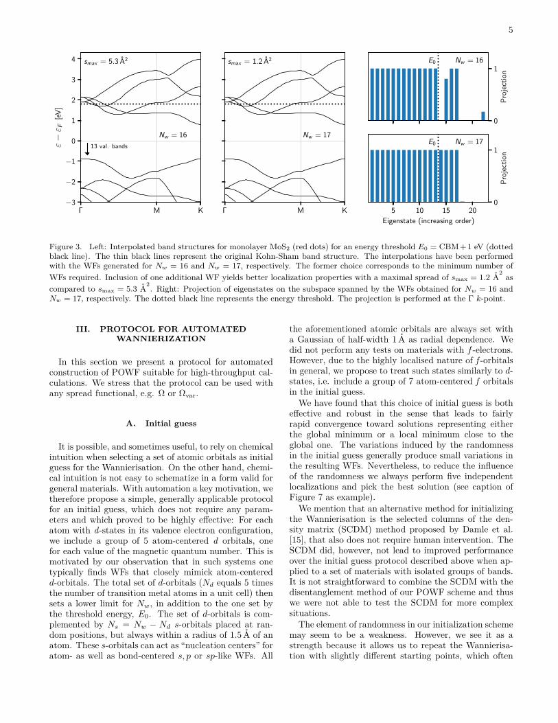
To illustrate how the Nw parameter may influence theWannierisation, we consider the case of monolayer MoS2.In Fig. 3(left) we show the interpolated band structureobtained from the POWFs obtained by maximising theΩ spread functional. Results are shown with an energythreshold (E0) of 1 eV above the conduction band min-imum (CBM) for Nw = 16 and Nw = 17, respectively.(The choice Nw = 16 corresponds to the minimum num-ber of WFs because exactly 16 bands fall below E0 at ap-proximately 1/3 along the Γ-M path.) It is clear that thechoice Nw = 17 improves both the band structure inter-polation and smax. In the present case, this result couldhave been anticipated by an analysis of the band struc-ture, which present an energy gap separating the lowest17 bands from all higher lying bands. Fig. 3(right) showsresolution of the resulting set of WF over the eigenstates(at the Γ point). From this analysis it is clear, that thetarget states, consisting of states below E0, can be per-fectly completed by including the lowest 17 bands in theWannierization. In contrast, a frustrated solution is ob-tained for Nw = 16 where one of the EDF becomes a mixof eigenstate 15 and 22.

In general, the effect of varying Nw can be difficultto predict. A prototype example where this happens isa non-elemental, low symmetry material with no natu-ral band gaps above E0. In such cases, the POWF lo-calization algorithm, which may be seen as a bonding-antibonding completion procedure, might select EDFcorresponding to high-energy eigenstates well separatedfrom the target bands, or even mixtures of such [5].

D. Initial guess

The iterative localization procedure requires an initialguess for the rotation matrix U and the EDF coefficientmatrix c. The quality of the initial guess is essential. Thisis particularly true for systems with many WFs wherethe iterative optimization algorithm is more likely to gettrapped in a local minimum if the initial guess is far fromthe global minimum. A natural choice is to start from aset of NAO atomic orbitals gi, and then project theseonto the available eigenstates, producing the Nb × NAOmatrix Pni = 〈ψn|gi〉. A prescription for extracting Uand c from P can be found in Ref. [5]. We not thatNAO = Nw in this procedure.

5

Γ M K−3

−2

−1

0

1

2

3

4ε−ε F

[eV]

smax = 5.3 A2

Nw = 1613 val. bands

Γ M K

smax = 1.2 A2

Nw = 170

1

Proj

ectio

n

Nw = 16E0

5 10 15 20Eigenstate (increasing order)

0

1

Proj

ectio

n

Nw = 17E0

Figure 3. Left: Interpolated band structures for monolayer MoS2 (red dots) for an energy threshold E0 = CBM+1 eV (dottedblack line). The thin black lines represent the original Kohn-Sham band structure. The interpolations have been performedwith the WFs generated for Nw = 16 and Nw = 17, respectively. The former choice corresponds to the minimum number ofWFs required. Inclusion of one additional WF yields better localization properties with a maximal spread of smax = 1.2 A2 ascompared to smax = 5.3 A2. Right: Projection of eigenstates on the subspace spanned by the WFs obtained for Nw = 16 andNw = 17, respectively. The dotted black line represents the energy threshold. The projection is performed at the Γ k-point.

III. PROTOCOL FOR AUTOMATEDWANNIERIZATION

In this section we present a protocol for automatedconstruction of POWF suitable for high-throughput cal-culations. We stress that the protocol can be used withany spread functional, e.g. Ω or Ωvar.

A. Initial guess

It is possible, and sometimes useful, to rely on chemicalintuition when selecting a set of atomic orbitals as initialguess for the Wannierisation. On the other hand, chemi-cal intuition is not easy to schematize in a form valid forgeneral materials. With automation a key motivation, wetherefore propose a simple, generally applicable protocolfor an initial guess, which does not require any param-eters and which proved to be highly effective: For eachatom with d-states in its valence electron configuration,we include a group of 5 atom-centered d orbitals, onefor each value of the magnetic quantum number. This ismotivated by our observation that in such systems onetypically finds WFs that closely mimick atom-centeredd-orbitals. The total set of d-orbitals (Nd equals 5 timesthe number of transition metal atoms in a unit cell) thensets a lower limit for Nw, in addition to the one set bythe threshold energy, E0. The set of d-orbitals is com-plemented by Ns = Nw − Nd s-orbitals placed at ran-dom positions, but always within a radius of 1.5 A of anatom. These s-orbitals can act as “nucleation centers” foratom- as well as bond-centered s, p or sp-like WFs. All

the aforementioned atomic orbitals are always set witha Gaussian of half-width 1 A as radial dependence. Wedid not perform any tests on materials with f -electrons.However, due to the highly localised nature of f -orbitalsin general, we propose to treat such states similarly to d-states, i.e. include a group of 7 atom-centered f orbitalsin the initial guess.

We have found that this choice of initial guess is botheffective and robust in the sense that leads to fairlyrapid convergence toward solutions representing eitherthe global minimum or a local minimum close to theglobal one. The variations induced by the randomnessin the initial guess generally produce small variations inthe resulting WFs. Nevertheless, to reduce the influenceof the randomness we always perform five independentlocalizations and pick the best solution (see caption ofFigure 7 as example).

We mention that an alternative method for initializingthe Wannierisation is the selected columns of the den-sity matrix (SCDM) method proposed by Damle et al.[15], that also does not require human intervention. TheSCDM did, however, not lead to improved performanceover the initial guess protocol described above when ap-plied to a set of materials with isolated groups of bands.It is not straightforward to combine the SCDM with thedisentanglement method of our POWF scheme and thuswe were not able to test the SCDM for more complexsituations.

The element of randomness in our initialization schememay seem to be a weakness. However, we see it as astrength because it allows us to repeat the Wannierisa-tion with slightly different starting points, which often

6

leads to slightly different outcomes of which the ”best”solution can be selected. The results in Fig. 4 showthe presence of multiple nearby local maxima of both Ωand Ωvar for bulk silicon. In this case, all the solutionsare valid in the sense that the WFs are all well localizedand real valued. Nonetheless, in a given situation onemay prefer a specific solution satisfying certain problemspecific requirements. The figure also clearly reveals theconsistent reduction of the maximum spread smax whenusing the Ωvar functional, in particular when used witha non-optimal Nw, such as the minimum value. The im-provement becomes less pronounced in this case whenusing the optimal Nw. A more detailed discussion ofthese aspects are provided in Sec. IV D.

B. Optimal number of Wannier functions

When the optimal number of WFs cannot be guessed,c.f. Sec. II C, it must be computed. We do this byconstructing the POWFs for a range of Nw ≥ Nmin

w andselecting the solution presenting the smallest smax. Inother words, we add EDF to the Wannierization space aslong as it reduces the spread of the least localized WF.For the calculations presented in this work we have var-ied Nw from Nmin

w to Nminw +5. Depending on the size of

the system (number of bands) and the available compu-tational resources, a higher upper limit may be chosen.Due to the randomness in the initial guess, we run 5optimizations for each value of Nw and select the bestsolution. In total we thus perform 25 Wannierisations

3.3 3.4 3.5

2.54

2.55

2.56

Aver

age

spre

ad[A

2 ]

Si (FCC)Minimal Nw

E0 = CBM + 2 eVΩΩvar

1.70 1.75 1.80Maximum spread [A2]

1.60

1.62

1.64

Aver

age

spre

ad[A

2 ]

Si (FCC)Optimal Nw

E0 = CBM + 2 eVΩΩvar

Figure 4. Spread distribution of several calculations withdifferent random seeds for the initial guess. Each data pointrepresents the result of a single calculation, for a total of 100for each functional.

6 7 8 9 10Total number of WFs

1.5

2.0

2.5

3.0

3.5

4.0

Max

imum

spre

ad[A

2 ] GaAs (FCC)E0 = CBM + 2 eV

−4

−2

0

2

4

ε−ε F

[eV]

Nw = 6

Γ X W K Γ L−4

−2

0

2

4ε−ε F

[eV]

Nw = 8

Figure 5. Top: The spread of the most delocalized WFobtained for GaAs(FCC) for different values of Nw. The cal-culations for each value of Nw have been repeated 5 timeswith different initial orbitals. The circles indicate the aver-age value and the error bars are the standard deviation overthe 5 independent Wannierisations. Bottom: Interpolatedband structure of GaAs obtained using the minimal Nw = 6(as defined by the energy threshold of E0 = CBM + 2 eV)and the optimal Nw = 8. The thin black lines represent theKohn-Sham band structure, the red dots are the Wannier in-terpolation.

for each material. Based on our experience, the resultingoptimal Nw is the same for Ω and Ωvar.

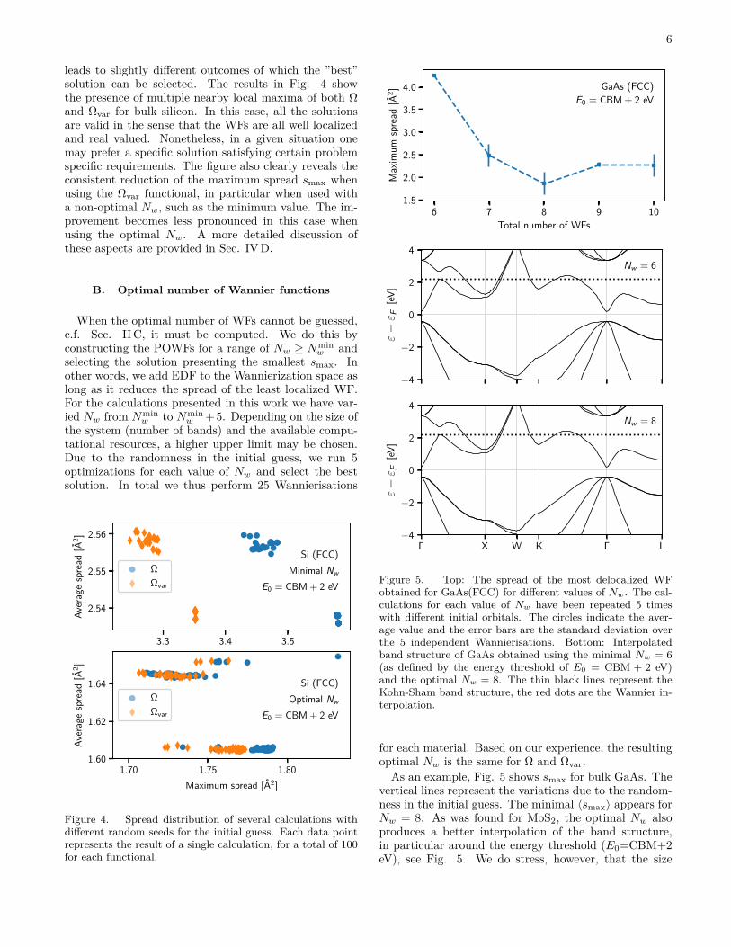
As an example, Fig. 5 shows smax for bulk GaAs. Thevertical lines represent the variations due to the random-ness in the initial guess. The minimal 〈smax〉 appears forNw = 8. As was found for MoS2, the optimal Nw alsoproduces a better interpolation of the band structure,in particular around the energy threshold (E0=CBM+2eV), see Fig. 5. We do stress, however, that the size

7

of smax is not always directly correlated with the bandinterpolation error[6, 16].

IV. RESULTS

In this section we present the results we obtained withour methods. We start presenting the differences we ob-served with the new localization functional on few specificsystems, then we move to a verification of the automatedprocedure on a set of 30 two-dimensional materials.

A. An illustrative example: WMo3Te8

In order to demonstrate the effect of the variance termin our newly defined localization functional Ωvar, we con-struct the Wannier functions of monolayer WMo3Te8.This material is a 2D semiconductor with 12 atoms perunit cell, 52 occupied bands, and a band gap of 0.9 eVobtained from a DFT calculation with the PBE xc-functional [7, 17].

In particular, we set an energy threshold E0 = CBM+2eV and computed 64 WFs, that is the minimal number ofWFs needed to describe the states up to E0. The largenumber of WFs helps in proving our thesis, the optimiza-tion algorithm is in fact more likely to choose a solutionwith few delocalized WFs, if the relative contribution tothe total localization functional is lower.

For monolayer WMo3Te8 we obtain an average spread(see App. A) of s = 2.7 A2 and a maximum spread ofsmax = 21.5 A2 with the standard functional Ω, while thevariance minimizing functional Ωvar converges to s = 2.8A2 and smax = 5.1 A2. The most delocalized WFs forboth functionals are shown in Figure 6. For the bandstructure interpolation error (see App. B) we obtainη = 21 meV (ηmax = 420 meV) for the standard ML-WFs produced by Ω and η = 9 meV (ηmax = 143 meV)for the spread balanced WFs generated with Ωvar.

As expected, the average localization of the WFs gen-erated with the two different spread functionals is almostidentical while the spread of the most delocalized WFs isgreatly improved by Ωvar. Moreover, the variance reduc-ing functional leads to a significant improvement in thetight-binding interpolation of the band structure. Westress that the significant improvements found with Ωvarfor this specific material may not be fully representative.Although we do generally find a significant improvement,i.e. reduction, of smax, the band interpolation error is of-ten similar to that obtained with Ω (see Sec. IV D).

The effect of the variance penalty term on the opti-mization of Ωvar is plotted in Figure 6 (c). Comparingthe value of the variance term between the two itera-tive optimizations, with Ω and Ωvar, it is clear that thepenalty term leads to a different convergence path. Forthe vast majority of the materials we tested, the numberof steps required for the optimization of Ωvar was compa-

c)

Figure 6. Isosurface plots of the most delocalized WF ofmonolayer WMo3Te8 obtained with (a) the standard local-ization functional Ω yielding a spread of smax = 21.5 A2 and(b) the variance reducing functional Ωvar yielding a spread ofsmax = 5.1 A2. The Wannierisation has been performed forthe minimal number of WFs consistent with an energy thresh-old of E0 = CBM + 2 eV. The isosurface level is 0.7 A−3/2.(c) The value of the variance penalty term in Ωvar (see Eq.(6)) during the iterative optimization. Additional optimiza-tion steps with Ωvar can further decrease the variance termby a factor of 2.

rable to or slightly larger than required for Ω. However,due to the additional terms in the gradient of Ωvar, eachstep is roughly twice as expensive to evaluate in termscomputational time.

8

B. Spontaneous polarization

The spontaneous polarization of ferrolectrics comprisesa prominent example of a physical quantity that is easilyaccessible from Wannier functions. As shown by King-Smith and Vanderbilt [8] the change in polarization underan adiabatic deformation can be calculated by a Berry-phase type formula. Typically the polarization of ferro-electrics is measured with respect to a centrosymmetricphase which is known to have vanishing polarization andthe spontaneous polarization can then be computed by asingle calculation in the polar phase.

To unravel the relation to Wannier functions it isstraightforward to show that the Wannier charge centerscan be written as [14]

rn ≡ 〈wn |r|wn〉 = V

(2π)3

∫dk〈unk|i∇k|unk〉, (8)

where V is the unit cell volume and unk is the periodicpart of a Bloch function. Except for the factor of Vthis expression is exactly the Berry phase formula forthe electric contribution to the polarization for a singleband and the full polarization can thus be written as

P = 1V

∑a

Zara −1V

∑n∈occ

rn, (9)

where ra is the position of nucleus a with charge Za. Eq.(9) is formally equivalent to the Berry phase expressionfor the polarization and the 2π ambiguity in the Berryphase is reflected by the fact that the nuclei positionsas well as the Wannier functions can be chosen in anarbitrary unit cell. This expression for the polarizationhas the advantage of providing a clear physical interpre-tation of the polarization as the dipole resulting from adiplacement of Wannier charge centers from the nucleipositions. Moreover, it strongly facilitates a microscopicanalysis of how the polarization is affected by impuritiesor interfaces since one may monitor the shift in Wanniercharge centers under an applied perturbation.

We have compared the calculated spontaneous polar-ization of tetragonal BaTiO3 obtained with a direct im-plementation of the Berry phase method [18] with thatobtained from Eq. (9) using the Ωvar spread functionalEq. (6) to construct Wannier functions from the occu-pied states. In the present case we have performed afull relaxation with the PBE functional using a 8× 8× 8k-point mesh and 800 eV plane wave cutoff. The resultfrom both calculations is 45.4 µC/cm2, which is in agree-ment with previous calculations [19, 20]. As expected,the new type of spread balanced Wannier functions thusreproduce the result obtained with standard maximallylocalized Wannier functions.

C. Complex systems

While the generation of well localized Wannier func-tions is usually relatively straightforward for simple sys-

tems (small number of atoms, isolated group of bands,etc.), it can be significantly more challenging in the gen-eral case. To test the variance reducing localization func-tional on more complex systems we compare its per-formance to the standard Ω functional for a nitrogen-vacancy (NV) defect center in a diamond crystal and aRu(111) surface slab with adsorbed H, N, and O atoms,respectively. The results are summarized in Table Iand confirm the previous conclusions. In particular, thespread of the most delocalized WF is significantly re-duced when using the Ωvar functional.

Additional computational details are provided in App.D.

D. Towards high-throughput applications

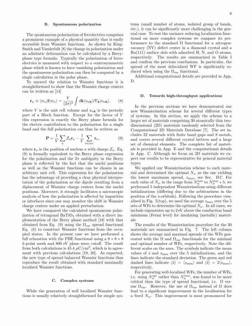
In the previous sections we have demonstrated ournew Wannierisation scheme for several different typesof systems. In this section, we apply the scheme to alarger set of materials comprising 30 atomically thin two-dimensional (2D) materials randomly selected from theComputational 2D Materials Database [7]. The set in-cludes 22 materials with finite band gaps and 8 metals,and covers several different crystal lattices and a largeset of chemical elements. The complete list of materi-als is provided in App. E and the computational detailsin App. C. Although we focus on 2D materials we ex-pect our results to be representative for general materialtypes.

We applied our Wannierisation scheme to each mate-rial and determined the optimal Nw as the one yieldingthe lowest maximum spread, smax, see Sec. II C. Foreach value of Nw in the range from Nmin

w to Nminw +5, we

performed 5 independent Wannierisations using differentinitializations (differing due to the arbitrariness in theposition of the s-orbitals). Following the procedure visu-alised in Fig. 5(top), we used the average smax over the 5sets of WFs to determine the optimal Nw. In all cases, weinclude eigenstates up to 2 eV above the conduction bandminimum (Fermi level) for insulating (metallic) materi-als.

The results of the Wannierisation procedure for the 30materials are summarised in Fig. 7. The left columnshows the average and maximal spreads of the WFs gen-erated with the Ω and Ωvar functionals for the minimaland optimal number of WFs, respectively. Note the dif-ferent scales on the axes. The symbols indicate the meanvalues of s and smax over the 5 initializations, and thelines indicate the standard deviation. The green and reddashed lines indicate 〈s〉 = 〈smax〉 and 〈s〉 = 2〈smax〉,respectively.

For generating well-localized WFs, the number of WFs,i.e. using Nopt

w rather than Nminw , was found to be more

critical than the type of spread functional, i.e. Ω ver-sus Ωvar. However, the use of Ωvar instead of Ω doeslead to a significant improvement in the localisation fora fixed Nw. This improvement is most pronounced for

9

0 5 10 15 20 25Maximum spread [A2]

0.5

1.0

1.5

2.0

2.5

3.0Av

erag

esp

read

[A2 ]

ΩMinimal Nw

0 50 100 150 200 250 300 350 400Maximum band interpolation error [meV]

0

10

20

#of

mat

erial

s

Ω

Minimal Nw

0 2 4 6 8 10Maximum spread [A2]

0.5

1.0

1.5

2.0

2.5

3.0

Aver

age

spre

ad[A

2 ]

ΩOptimal Nw

0 50 100 150 200 250 300 350 400Maximum band interpolation error [meV]

0

10

20

#of

mat

erial

s

Ω

Optimal Nw

0 2 4 6 8 10Maximum spread [A2]

0.5

1.0

1.5

2.0

2.5

3.0

Aver

age

spre

ad[A

2 ]

ΩvarMinimal Nw

0 50 100 150 200 250 300 350 400Maximum band interpolation error [meV]

0

10

20

#of

mat

erial

s

Ωvar

Minimal Nw

0 2 4 6 8 10Maximum spread [A2]

0.5

1.0

1.5

2.0

2.5

3.0

Aver

age

spre

ad[A

2 ]

ΩvarOptimal Nw

0 50 100 150 200 250 300 350 400Maximum band interpolation error [meV]

0

10

20

#of

mat

erial

s

Ωvar

Optimal Nw

Figure 7. Results for the set of 2D materials with different choices for Nw and the localization functional. The energy thresholdis set at CBM (EF ) + 2 eV for insulators (metals). Left column: Spread of WFs for all the materials in the test set averagedover 5 runs with different initializations. The standard deviation is indicated by lines. The dashed green line is smax = s, thedotted red line is smax = 2s. The red circles indicate results for WMo3Te8 and ZrTi3Te8. Right column: The maximum bandinterpolation error. Results from the most localized set of WFs, out of the 5 calculations with different random seeds.

10

Ω Ωvar

System Nw 〈smax〉 [A2] ηmax [meV] 〈smax〉 [A2] ηmax [meV]

NV center in diamond 127 6.8± 0.3 8 4.46± 0.04 8Adsorbed H on Ru slab 133 8± 1 158 4.6± 0.5 172Adsorbed N on Ru slab 134 6.8± 0.7 89 4.6± 0.6 82Adsorbed O on Ru slab 135 6.9± 0.5 77 4.7± 0.4 117

Table I. Comparison of the spread of the most delocalized WF and the maximum band interpolation error obtained for WFsgenerated with the standard spread functional Ω and the variance reducing functional Ωvar for the NV center in diamondand H, N, O adsorbed on a Ru(111) surface slab. The minimal Nw was used for all materials. 〈smax〉 is the average over 5calculations with different random seeds (standard deviation also shown). ηmax is the maximum band interpolation error forthe most localized set of WFs (lowest maximum spread) obtained in the 5 calculations with different random seeds.

non-optimal values of Nw, e.g. the minimal Nw. In par-ticular, for the two materials WMo3Te8 and ZrTi3Te8(both with Nw > 60 and indicated by red circles), wewere not able to localize all the WFs when using the Ω-functional and the minimal Nw. This issue did not occurwith the Ωvar-functional. Even when using the optimalNw, the improvement by the Ωvar-functional is signifi-cant. Not only do we obtain better localisation of theleast localised WF (smax) without sacrificing the averagelocalisation (s), the standard deviations on both s andsmax is also lowered.

The band interpolation errors (again averaged over the5 initializations) are shown in the right column of Fig. 7.As previously found and discussed in Section III B, the er-rors decrease significantly when using the optimized Nwas compared to the minimal Nw. With the optimal Nwthe majority of the materials show a maximum error be-low 20 meV. A few materials show higher band errors,which is related to significant band crossings (band en-tanglement) with higher energy bands close to the E0energy cutoff. We note in passing that if accurate bandinterpolation in this region is required, one may simplyincrease E0, which will push the inaccuracies to higherband energies.

While the Ωvar spread functional improves the localisa-tion properties of WFs, it does not represent a significantimprovement over Ω in terms of the band interpolationerror. This shows that the band interpolation error is notdirectly correlated with the localisation properties of theWFs. More precisely, it is not directly correlated with thespread of the most delocalised WF, smax, which is alwayssignificantly and consistently reduced by using Ωvar. Westress, however, that there are many other applicationsof WFs where robust localisation of all WFs, is of keyimportance. These include the interpolation of electron-phonon matrix elements[21, 22], calculation of Berry cur-vatures and conductivities[23], and basis sets for electrontransport calculations based on non-equilibrium Green’sfunctions[24, 25].

The effect of penalizing the spread variance in Ωvar canbe illustrated by considering the localisation propertiesof the resulting sets of WFs averaged over all 30 materi-als for a fixed Nw. Specifically, we fix Nw at either its

minimal or optimal value, and consider the mean of theaverage spread

〈〈s〉init〉mat = 1Nmat

Nmat∑m=1

(1

Ninit

Ninit∑i=1

smi

)(10)

and the mean standard deviation of the average spreadover 5 initialisations

〈σinit(s)〉mat = 1Nmat

Nmat∑m=1

√Varinit[smi ], (11)

whereNmat is the total number of materials (hereNmat =30), Ninit is the number of independent optimizationswith different initial guess (here Ninit = 5), smi is theaverage spread of the WFs of material m with initializa-tion i, and Varinit is the variance of the Ninit independentruns. In the same way, we can define 〈〈smax〉init〉mat and〈σinit(smax)〉mat by replacing s with smax in the aboveequations. Note, that 〈σinit(s)〉mat and 〈σinit(smax)〉matmeasure the variation in the average and maximal spreadin dependence of the initial guess, i.e. the robustness ofthe Wannierisation. In particular, it does not reflect thevariation of the spreads within a given set of WFs. Asdemonstrated on several places in the paper, the latter isalways significantly and consistently reduced when usingΩvar.

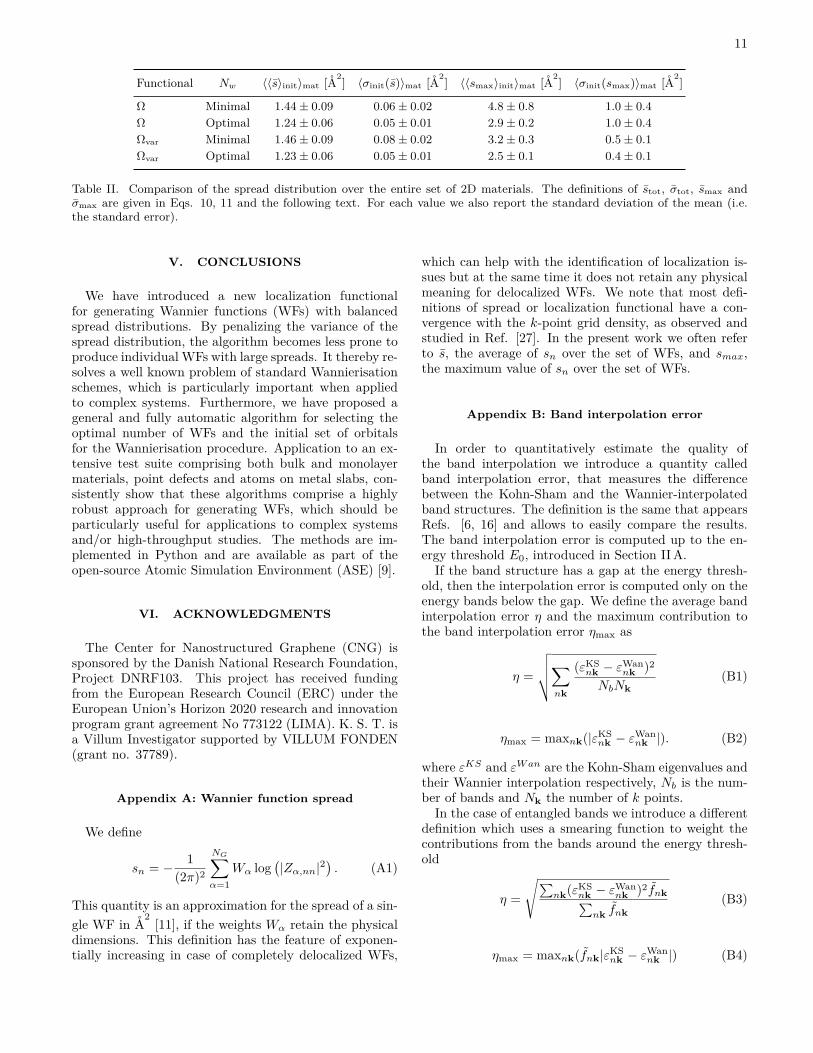
Table II shows the results for the four quan-tities 〈〈s〉init〉mat, 〈〈smax〉init〉mat, 〈σinit(s)〉mat, and〈σinit(smax)〉mat for each of the spread functionals Ω andΩvar. These numbers summarise the information in Fig.7. On this basis we conclude that the penalization of thespread variance as done in the Ωvar-functional, does notaffect the average spread of the WFs, but consistentlydecreases the maximum spread and improves the robust-ness with respect to the choice of initial orbitals.

E. Data availability

The data presented in this article together with infor-mation required for its reproduction, are available in anonline open access archive [26]. For more details see alsoApp. F.

11

Functional Nw 〈〈s〉init〉mat [A2] 〈σinit(s)〉mat [A2] 〈〈smax〉init〉mat [A2] 〈σinit(smax)〉mat [A2]

Ω Minimal 1.44± 0.09 0.06± 0.02 4.8± 0.8 1.0± 0.4Ω Optimal 1.24± 0.06 0.05± 0.01 2.9± 0.2 1.0± 0.4Ωvar Minimal 1.46± 0.09 0.08± 0.02 3.2± 0.3 0.5± 0.1Ωvar Optimal 1.23± 0.06 0.05± 0.01 2.5± 0.1 0.4± 0.1

Table II. Comparison of the spread distribution over the entire set of 2D materials. The definitions of stot, σtot, smax andσmax are given in Eqs. 10, 11 and the following text. For each value we also report the standard deviation of the mean (i.e.the standard error).

V. CONCLUSIONS

We have introduced a new localization functionalfor generating Wannier functions (WFs) with balancedspread distributions. By penalizing the variance of thespread distribution, the algorithm becomes less prone toproduce individual WFs with large spreads. It thereby re-solves a well known problem of standard Wannierisationschemes, which is particularly important when appliedto complex systems. Furthermore, we have proposed ageneral and fully automatic algorithm for selecting theoptimal number of WFs and the initial set of orbitalsfor the Wannierisation procedure. Application to an ex-tensive test suite comprising both bulk and monolayermaterials, point defects and atoms on metal slabs, con-sistently show that these algorithms comprise a highlyrobust approach for generating WFs, which should beparticularly useful for applications to complex systemsand/or high-throughput studies. The methods are im-plemented in Python and are available as part of theopen-source Atomic Simulation Environment (ASE) [9].

VI. ACKNOWLEDGMENTS

The Center for Nanostructured Graphene (CNG) issponsored by the Danish National Research Foundation,Project DNRF103. This project has received fundingfrom the European Research Council (ERC) under theEuropean Union’s Horizon 2020 research and innovationprogram grant agreement No 773122 (LIMA). K. S. T. isa Villum Investigator supported by VILLUM FONDEN(grant no. 37789).

Appendix A: Wannier function spread

We define

sn = − 1(2π)2

NG∑α=1

Wα log(|Zα,nn|2

). (A1)

This quantity is an approximation for the spread of a sin-gle WF in A2 [11], if the weights Wα retain the physicaldimensions. This definition has the feature of exponen-tially increasing in case of completely delocalized WFs,

which can help with the identification of localization is-sues but at the same time it does not retain any physicalmeaning for delocalized WFs. We note that most defi-nitions of spread or localization functional have a con-vergence with the k-point grid density, as observed andstudied in Ref. [27]. In the present work we often referto s, the average of sn over the set of WFs, and smax,the maximum value of sn over the set of WFs.

Appendix B: Band interpolation error

In order to quantitatively estimate the quality ofthe band interpolation we introduce a quantity calledband interpolation error, that measures the differencebetween the Kohn-Sham and the Wannier-interpolatedband structures. The definition is the same that appearsRefs. [6, 16] and allows to easily compare the results.The band interpolation error is computed up to the en-ergy threshold E0, introduced in Section II A.

If the band structure has a gap at the energy thresh-old, then the interpolation error is computed only on theenergy bands below the gap. We define the average bandinterpolation error η and the maximum contribution tothe band interpolation error ηmax as

η =

√√√√∑nk

(εKSnk − εWan

nk )2

NbNk(B1)

ηmax = maxnk(|εKSnk − εWan

nk |). (B2)

where εKS and εWan are the Kohn-Sham eigenvalues andtheir Wannier interpolation respectively, Nb is the num-ber of bands and Nk the number of k points.

In the case of entangled bands we introduce a differentdefinition which uses a smearing function to weight thecontributions from the bands around the energy thresh-old

η =

√∑nk(εKS

nk − εWannk )2fnk∑

nk fnk(B3)

ηmax = maxnk(fnk|εKSnk − εWan

nk |) (B4)

12

where fnk =√fKSnk (ν, τ)fWan

nk (ν, τ) and fnk(ν, τ) is theFermi-Dirac distribution for the state at energy εnk, νis a fictitious chemical potential fixed at E0 and τ is asmearing width fixed to 0.1 eV.

Appendix C: Computational details

For each material in this work we performed a self-consistent PBE calculation with the GPAW code[28] us-ing a Monkhorst-Pack grid [29] with a minimum densityof 5 k-points per A−1 and a real-space grid with a spac-ing of 0.2 A. Several unoccupied states were included inthe calculation. The band structure calculation, used toevaluate the band interpolation accuracy, was performedby fixing the density to the value from the previous self-consistent calculation and evaluating the band structurealong a path with minimum density of 50 k-points perA−1. Finally, we computed the WFs with ASE [9], start-ing from the self-consistent DFT Bloch states. For allmaterials in Sec. IV D we used the structure available inthe public C2DB database [7].

Appendix D: Methods for complex systems

For the NV center in diamond we substituted one car-bon atom with a nitrogen atom in a 64 atom cubic unitcell of bulk diamond. We then proceeded in the structurerelaxation using GPAW [28], with a 2x2x2 Monkhorst-Pack grid of k-points in the Brillouin zone (BZ), a planewaves basis set with an energy cutoff of 400 eV and aninitial charge of −1. The structure was optimized withthe LBFGS algorithm [30] and the force threshold was setto 0.05 eV A−1. After the structure was relaxed we ran aself-consistent and a non self-consistent calculation, witha BZ sampling density of 2 and 5 k-points per A−1 re-spectively. The self-consistent calculation was convergedfor every state up to 4 eV from the conduction band min-imum (CBM). The rest of the methods were in line with

Section IV D.With the adsorption systems we followed a similar

workflow with ASE [9]. We created a 2x2x4 slab of ruthe-nium with HCP(0001) surface and a vacuum layer of 7 Aalong the z direction. Then the adsorbate was placed onthe HCP site at 1 A, 1.108 A, 1.257 A for H, N, O respec-tively. The structure was then relaxed, fixing the first twolayers of Ru, using the finite-difference method and thePBE [17] xc-functional in GPAW, again using LBFGS asoptimization algorithm and 0.05 eV A−1 as forces thresh-old. After the relaxation, a self-consistent and a nonself-consistent calculations were ran on each system, fol-lowing the workflow for the NV center in diamond.

Appendix E: List of 2D materials

The 2D structures in Table III are picked from theC2DB database [7]. The values for the maximum spreadare the mean and the standard deviation over 5 calcu-lations with different random seeds for the initial guess.The standard deviation for the maximum band interpo-lation error is computed with the same method. For themaximum band interpolation and the number of WFs(the latter varies only in the case of optimal Nw) we usethe value from the most localized set (lowest maximumspread) over 5 calculations, instead of the mean value. Inthe last row we show the average value and the averagestandard deviation for each column.

Appendix F: Software availability

Most of the software used and developed in this projectis open-source and available for free. The density func-tional theory code used is GPAW 20.10 [28] with version0.9.2 of the atomic setups, together with ASE 3.20 [9].The latter also includes the Wannier module in whichthe new spread functional has been implemented. TheWannier functions are represented with Vesta [31], whichis available for free. The plots are produced with Mat-plotlib [32] and the independent calculations were run inparallel with the help of GNU parallel [33], both of themare open-source software.

[1] G. H. Wannier, Phys. Rev. 52, 191 (1937).[2] N. Marzari and D. Vanderbilt, Phys. Rev. B 56, 12847

(1997).[3] K. S. Thygesen, L. B. Hansen, and K. W. Jacobsen, Phys.

Rev. Lett. 94, 026405 (2005).[4] I. Souza, N. Marzari, and D. Vanderbilt, Phys. Rev. B

65, 035109 (2001).[5] K. S. Thygesen, L. B. Hansen, and K. W. Jacobsen, Phys.

Rev. B 72, 125119 (2005).[6] A. Damle, A. Levitt, and L. Lin, Multiscale Modeling &

Simulation 17, 167 (2019).[7] S. Haastrup, M. Strange, M. Pandey, T. Deilmann, P. S.

Schmidt, N. F. Hinsche, M. N. Gjerding, D. Torelli, P. M.

Larsen, A. C. Riis-Jensen, J. Gath, K. W. Jacobsen, J. J.Mortensen, T. Olsen, and K. S. Thygesen, 2D Materials5, 042002 (2018).

[8] R. D. King-Smith and D. Vanderbilt, Phys. Rev. B 47,1651 (1993).

[9] A. H. Larsen, J. J. Mortensen, J. Blomqvist, I. E.Castelli, R. Christensen, M. Du lak, J. Friis, M. N.Groves, B. Hammer, C. Hargus, E. D. Hermes, P. C.Jennings, P. B. Jensen, J. Kermode, J. R. Kitchin, E. L.Kolsbjerg, J. Kubal, K. Kaasbjerg, S. Lysgaard, J. B.Maronsson, T. Maxson, T. Olsen, L. Pastewka, A. Pe-terson, C. Rostgaard, J. Schiøtz, O. Schutt, M. Strange,K. S. Thygesen, T. Vegge, L. Vilhelmsen, M. Walter,

13

Minimal Nw / Ω Optimal Nw / Ωvar

Formula Crystal type Nw 〈smax〉 [A2] ηmax [meV] Nw 〈smax〉 [A2] ηmax [meV]

Ag2Br2 AB-129-bc 26 2.3± 0.5 11.7± 0.2 26 1.7± 0.7 11.6± 0.1Al2Cl2O2 ABC-59-ab 20 4.3± 0.2 13± 3 23 3.6± 0.2 5.0± 0.7Au2S2 AB-10-fgm 19 3.21± 0.08 24± 5 22 2.6± 0.1 5± 3BrClTi ABC-59-ab 18 2.43± 0.01 5.1± 0.1 18 2.44± 0.09 5.2± 0.3Br2Hf2S2 ABC-156-ac 29 6.3± 0.3 373± 6 32 1.57± 0.07 105.3± 0.4C2H2 AB-164-d 8 5.0± 0.5 13.3± 0.4 8 4.9± 0.7 8± 2CF2Y2 AB2C2-164-bd 23 6.9± 0.5 36± 1 27 3.2± 0.2 18± 4CH2O2V2 AB2C2D2-164-bd 31 5.3± 1.6 111± 58 35 3.0± 0.6 254± 75Cl2Sc2Se2 ABC-59-ab 32 1.64± 0.05 6.3± 0.1 33 1.9± 0.7 6.5± 0.6Cr2W2S8 ABC4-28-bcd 56 7± 11 8± 48 59 2± 1 5.2± 0.9CSiH2 ABC2-156-ab 9 5.763± 0.001 6± 2 13 4.15± 0.02 3.0± 0.6Hf2Cl4 AB2-11-e 30 4.74± 0.01 62± 1 34 2.67± 0.04 30± 1HgI2 AB2-115-dg 17 1.806± 0.001 2.9± 0.1 17 1.792± 0.001 2.9± 0.1I2O2Rh2 ABC-59-ab 32 1.63± 0.01 4.0± 0.1 35 2.0± 0.9 3± 280In2S2 AB-164-cd 22 6.83± 0.01 52± 2 26 2.4± 0.2 5± 2Ir2Br6 AB3-162-dk 40 1.303± 0.001 5.6± 0.1 41 1.32± 0.03 5.1± 0.2ISSb ABC-156-abc 17 6± 6 4.5± 74.0 17 2.5± 0.8 5± 2MoSe2 AB2-187-bi 17 1.63± 0.04 6.6± 0.1 17 3± 2 7± 32N2O2Zr3 A2B2C3-187-bghi 37 2.7± 0.3 9.5± 20.0 39 1.8± 0.7 9.2± 0.9Nb2I4 AB2-11-e 35 3.12± 0.01 100.1± 0.2 38 3.0± 0.3 97± 4PdS2 AB2-164-bd 13 1.26± 0.02 2.0± 0.1 13 2.5± 0.7 2.0± 0.6PtSe2 AB2-164-bd 16 1.652± 0.001 13.9± 0.1 18 2.3± 0.2 7± 5Ru2Se4 AB2-11-e 34 1.55± 0.01 9.2± 0.4 34 2.2± 0.7 8.0± 0.5ScSe2 AB2-164-bd 12 4± 5 8± 189 16 1.50± 0.01 1.8± 0.4SnTe2 AB2-164-bd 14 3.2± 0.4 16.6± 0.1 17 2.5± 0.9 15± 3SrCl2 AB2-164-bd 17 6.0± 0.8 0.8± 0.3 21 4.0± 0.2 1.2± 0.3TaS2 AB2-187-bi 13 5± 2 16± 470 17 1.6± 0.6 3.1± 0.1WMo3Te8 AB3C8-1-a 64 21.51± 0.06 420± 50 68 2.12± 0.05 10.6± 0.5WO2 AB2-187-bi 18 1.88± 0.01 1.8± 0.1 18 1.835± 0.002 1.8± 0.1ZrTi3Te8 AB3C8-1-a 58 18.77± 0.03 52± 4 62 2.29± 0.06 25± 7

Average - - 4.8± 0.8 47± 31 - 2.48± 0.15 22± 14

Table III. List of the 2D materials considered in Sec. IV D. The ”Crystal type” in the second column follows the convention ofthe C2DB database and stands for stoichiometry-space group-occupied Wyckoff positions.

Z. Zeng, and K. W. Jacobsen, Journal of Physics: Con-densed Matter 29, 273002 (2017).

[10] R. Resta and S. Sorella, Phys. Rev. Lett. 82, 370 (1999).[11] G. Berghold, C. J. Mundy, A. H. Romero, J. Hutter, and

M. Parrinello, Phys. Rev. B 61, 10040 (2000).[12] P. L. Silvestrelli, Phys. Rev. B 59, 9703 (1999).[13] J. M. Foster and S. F. Boys, Rev. Mod. Phys. 32, 300

(1960).[14] N. Marzari, A. A. Mostofi, J. R. Yates, I. Souza, and

D. Vanderbilt, Rev. Mod. Phys. 84, 1419 (2012).[15] A. Damle and L. Lin, Multiscale Modeling & Simulation

16, 1392 (2018).

[16] V. Vitale, G. Pizzi, A. Marrazzo, J. Yates, N. Marzari,and A. Mostofi, npj Computational Materials 6, 66(2020).

[17] J. P. Perdew, K. Burke, and M. Ernzerhof, Phys. Rev.Lett. 77, 3865 (1996).

[18] M. N. Gjerding, A. Taghizadeh, A. Rasmussen, S. Ali,F. Bertoldo, T. Deilmann, U. P. Holguin, N. R.Knøsgaard, M. Kruse, S. Manti, T. G. Pedersen,T. Skovhus, M. K. Svendsen, J. J. Mortensen, T. Olsen,and K. S. Thygesen, arxiv.org/abs/2102.03029 , 1 (2021),arXiv:2102.03029.

14

[19] I. E. Castelli, T. Olsen, and Y. Chen, Journal of Physics:Energy 2, 011001 (2019).

[20] U. Petralanda, M. Kruse, H. Simons, and T. Olsen,arxiv.org/abs/2012.11254 , 1 (2020), arXiv:2012.11254.

[21] F. Giustino, M. L. Cohen, and S. G. Louie, Physical Re-view B 76, 165108 (2007).

[22] J. Sjakste, N. Vast, M. Calandra, and F. Mauri, PhysicalReview B 92, 054307 (2015).

[23] X. Wang, J. R. Yates, I. Souza, and D. Vanderbilt, Phys-ical Review B 74, 195118 (2006).

[24] A. Calzolari, N. Marzari, I. Souza, and M. B. Nardelli,Physical Review B 69, 035108 (2004).

[25] M. Strange, I. S. Kristensen, K. S. Thygesen, and K. W.Jacobsen, The Journal of Chemical Physics 128, 114714(2008).

[26] P. F. Fontana and K. S. Thygesen, Robust wannier data(2021), 10.5281/zenodo.5338784.

[27] M. Stengel and N. A. Spaldin, Phys. Rev. B 73, 075121(2006).

[28] J. Enkovaara, C. Rostgaard, J. J. Mortensen, J. Chen,M. Du lak, L. Ferrighi, J. Gavnholt, C. Glinsvad,V. Haikola, H. A. Hansen, H. H. Kristoffersen,M. Kuisma, A. H. Larsen, L. Lehtovaara, M. Ljung-berg, O. Lopez-Acevedo, P. G. Moses, J. Ojanen,T. Olsen, V. Petzold, N. A. Romero, J. Stausholm-Møller, M. Strange, G. A. Tritsaris, M. Vanin, M. Walter,B. Hammer, H. Hakkinen, G. K. H. Madsen, R. M. Niem-inen, J. K. Nørskov, M. Puska, T. T. Rantala, J. Schiøtz,K. S. Thygesen, and K. W. Jacobsen, Journal of Physics:Condensed Matter 22, 253202 (2010).

[29] H. J. Monkhorst and J. D. Pack, Phys. Rev. B 13, 5188(1976).

[30] R. H. Byrd, P. Lu, J. Nocedal, and C. Zhu, SIAM Journalon Scientific Computing 16, 1190 (1995).

[31] K. Momma and F. Izumi, Journal of Applied Crystallog-raphy 44, 1272 (2011).

[32] J. D. Hunter, Computing in Science & Engineering 9, 90(2007).

[33] O. Tange, ;login: The USENIX Magazine 36, 42 (2011).