Spontaneous Parametric Down-Conversion and Quantum ... · Spontaneous Parametric Down-Conversion and Quantum Entanglement by Jesse Catalano An undergraduate honors thesis submitted

Portland State UniversityPDXScholar

University Honors Theses University Honors College

2014

Spontaneous Parametric Down-Conversion and QuantumEntanglementJesse L. CatalanoPortland State University

Let us know how access to this document benefits you.Follow this and additional works at: http://pdxscholar.library.pdx.edu/honorstheses

This Thesis is brought to you for free and open access. It has been accepted for inclusion in University Honors Theses by an authorized administrator ofPDXScholar. For more information, please contact [email protected].

Recommended CitationCatalano, Jesse L., "Spontaneous Parametric Down-Conversion and Quantum Entanglement" (2014). University Honors Theses. Paper52.

10.15760/honors.85

http://pdxscholar.library.pdx.edu?utm_source=pdxscholar.library.pdx.edu%2Fhonorstheses%2F52&utm_medium=PDF&utm_campaign=PDFCoverPages

http://pdxscholar.library.pdx.edu/honorstheses?utm_source=pdxscholar.library.pdx.edu%2Fhonorstheses%2F52&utm_medium=PDF&utm_campaign=PDFCoverPages

http://pdxscholar.library.pdx.edu/honors?utm_source=pdxscholar.library.pdx.edu%2Fhonorstheses%2F52&utm_medium=PDF&utm_campaign=PDFCoverPages

http://library.pdx.edu/services/pdxscholar-services/pdxscholar-feedback/

http://pdxscholar.library.pdx.edu/honorstheses?utm_source=pdxscholar.library.pdx.edu%2Fhonorstheses%2F52&utm_medium=PDF&utm_campaign=PDFCoverPages

http://pdxscholar.library.pdx.edu/honorstheses/52?utm_source=pdxscholar.library.pdx.edu%2Fhonorstheses%2F52&utm_medium=PDF&utm_campaign=PDFCoverPages

http://dx.doi.org/10.15760/honors.85

mailto:[email protected]

Spontaneous Parametric Down-Conversion and Quantum Entanglement

by

Jesse Catalano

An undergraduate honors thesis submitted in partial fulfillment of the

requirements for the degree of

Bachelor of Science

in

University Honors

and

Physics

Thesis Adviser

Andres La Rosa

Portland State University

2014

Table of Contents

Introduction…………………………………………………………..………………..3

1.1 Classical Theory of Spontaneous Parametric Down-Conversion (SPDC) –

Introduction……………………………………………………………..……..…..4

1.2 The Wave Equation……………………………………………………..………....5

1.3 Ordinary and Extraordinary Polarization Directions……………...….………..8

1.4 Non-linear Polarization and the [d] Matrix………………………….…………..9

1.5 Coupled Equations for Type-I and Type-II SPDC……………………………...11

2.1 Polarization Entanglement for Type-I and Type-II SPDC…………..…………13

2.2 Bell Inequality and Local-realism……………………………………..…………15

3.1 Quantum Teleportation using Entangled Photons……………………………...19

3.2 Entanglement Transfer from Photons to Matter….…………………………….21

Conclusion………………………………………………………………….………….23

Acknowledgments……………………………………………………………………..24

Appendix – Vector Orientation Relative to the Principle Axis……….….………....24

References………………………………………………………………….…………..25

Abstract

Quantum entanglement has been a topic of much research in modern physics, and an application

in quantum computing is envisioned. This thesis address the use of polarization entangled photon pairs

produced by spontaneous parametric down-conversion (SPDC) in entanglement transfer process and

quantum computing. The simplicity of SPDC entanglement relative to other quantum phenomena is

first emphasized by developing a complete classical theory of the photon-crystal interactions

characteristic of SPDC. The methods of achieving polarization superposition via the Type-I and Type-II

SPDC are described. A combination of superposition and polarization correlation between down-

converted photons is shown to violate Bell’s inequality, thus revealing the entangled nature of the

photon pairs. Finally, the possibility of controlling entangled photons through the manipulation of

surface plasmons is highlighted as a way to transfer entanglement from photons to material particles.

Introduction

Spontaneous parametric down-conversion (SPDC) is a 2nd

order optical effect where the dipole

polarization depends quadratically on the electric field and photons incident on a non-linear crystal can

be “converted” into two photons. It is an important process in quantum optics, used especially to

produce entangled photon pairs1, and also constitutes an excellent method to produce a source of single

photons2. An incident photon in SPDC is often referred to as the “pump” while the outgoing photons

are called the “signal” and “idler”. SPDC is said to be “spontaneous” because there is no input signal

or idler field to stimulate the process; they are generated spontaneously inside the crystal. The process

is “parametric” because it depends on the electric fields (and not just their intensities), implying that

there exists a phase relationship between input and output fields. “Down-conversion” refers to that fact

that the signal and idler fields always have a lower frequency than the pump.3 Splitting of the pump

photons into pairs of photons occurs in accordance with conservation laws, namely, having combined

energies and momenta equal to the energy and momentum of the original photon. These conservation

laws are given by

�� (1a)

�� , (1b)

where ω�, ω�, ω�, ��, ��, and ��, are the frequencies and wave vectors of the pump (subscript 3),

signal (subscript 1), and idler (subscript 2).

SPDC, as analyzed in this paper, is a phenomenon that requires photon-crystal interactions

among the three photons within a uniaxial crystal, where the pump photon is partially or fully polarized

in an extraordinary direction relative to the crystal’s optical axis. SPDC can be implemented in two

different varieties, characterized by the polarizations of the signal and idler. If both outgoing photons

are ordinary in their polarization it is deemed Type-I down-conversion. If one of the photons is

extraordinarily polarized while the other is ordinary, it is called Type-II. The possible paths of the

outgoing photons (schematically shown in Fig. 1) are determined by conservation laws and constraints

on polarization. In either case, the outgoing photons are correlated in their polarizations.

The direction of propagation for the signal and idler waves depend upon several factors, such as

their respective frequencies, the ordinary and extraordinary refractive indexes of the non-linear crystal,

no and ne, the angle between the pump and the crystal axis, and the conservation laws (1a) and (1b).

Additionally, the strength of the down-converted fields is determined by phase matching conditions4,

which are dependent upon crystal thickness and propagation speeds. Because propagation speeds

depend upon indices of refraction, Type-I and Type-II SPDC have different phase matching conditions.

Fig 1: The two types of Parametric Down-Conversion from a 2

nd order crystal. LEFT: Type-I down-conversion, where the

pump beam is converted into two beams with paths constrained to a cone centered on the pump. The output photons have

ordinary polarization relative to the crystal axis. RIGHT: Type-II down-conversion, where the pump beam is converted into

two beams which each appear anywhere on their respective cones, on opposite sides of the pump beam. One of the outgoing

photons will be ordinarily polarized, while the other will be extraordinary.

Both types can be attained by tuning the orientation of the non-linear crystal relative to the incident

beam direction. For example, in one experiment, Type-I SPDC was attained using a 413 nm pump

beam propagating at 28.3° from the crystal axis of a 1 mm thick BBO crystal (β-barium borate, β-

BaB2O4)5. In another experiment, Type-II SPDC was attained using a 341 nm pump at 49.6° from the

crystal axis of a 3 mm thick BBO crystal6.

The correlation between down-converted photon polarization states makes possible the

production of polarization-entangled photons. Entanglement is the quantum phenomenon where the

state a system of two or more particles is not determined by the states of the individual particles alone,

and only occurs when the particles of the system are in a quantum superposition of states and share a

correlation. If two photons are correlated in their polarizations, measuring the polarization state of one

determines the state of the other, without having to measure it. SPDC is adequate to produce photons

which are both correlated and in superposition. For Type-II, the outgoing photons are in superposition

where the cones intersect, because the polarization at that point is uncertain. For Type-I, two crystals

must be aligned in such a way that their cones overlap. This will be further explained in chapter 2 of

this paper.

In the first chapter of this paper, a theory of SPDC will be developed from first principles

(Maxwell’s equations). In chapter 2, the methods for attaining entanglement of photon polarizations for

both Type-I and Type-II SPDC will be given. It will also be shown that correlation between down-

converted photon polarizations puts into doubt local-realism, a viewpoint that considers reality as

deterministic, independent of the observer, and that no information travels faster than light.

Consequences of the violation of local-realism will be explored. Chapter 3 presents methods of

manipulating polarization entangled photons, and proposes a use for SPDC in entanglement transfer

experiments.

1.1 Classical Theory of SPDC - Introduction

We present here a theory of SPDC based on the Maxwell equations and the concept of non-

linear polarization. This treatment leads to three coupled equations for both Type-I and Type-II down-

conversion. The derivation of these equations requires many steps and several approximations. It is the

objective of this chapter to present a complete derivation of these coupled equations in a thorough and

logical manner. Throughout this chapter, it will be assumed that the non-linear crystal through which

SPDC occurs is KDP (KH2PO4). The results of this chapter can be extended to other uniaxial crystals.

1.2 The Wave Equation

Spontaneous parametric down-conversion (SPDC) is a 2nd

order optical effect which requires

non-linear uniaxial crystals. The behavior of light in a non-linear crystal can be determined from first

principles. We can begin with Maxwell's equations in matter. If we assume no electric currents or free

charges are present in the medium, then the electric field E, magnetic field B, and electric displacement

field D, are related by

�� (2)

�� , (3)

where µ is the permeability constant of the material. Given equation (3), the curl of equation (2) is

�� . (4)

The curl operators on the left side of equation (4) can be replaced using the following identity,

∇x∇xE E E E � ∇(∇⋅EEEE) - ∇2EEEE. (5)

In a linear material, the polarization P is related to the electric field by Plinear = ε0χlinearE, where ε0 is the

permittivity of a vacuum. Therefore, the electric displacement vector D ε0E + P in a linear material

can be written as D ε0E + P = ε0 (1+χlinear) E εE. In the non-linear case, P = Plinear + PNL = ε0χlinearE

+ PNL. Therefore, the electric displacement in a non-linear material is

� !"� � # � !� � #$%. (6)

Using equations (5) and (6), equation (4) can be written as

�� ( ⋅ �) �! ��

�� #$%. (7)

Equation (7) is a wave equation which explicitly shows how the polarization of a non-linear crystal is

related to the electric field within it. This equation holds for each vector component of any basis, hence,

projecting E and PNL on any particular axis results in a scalar relationship, which can be replace in

equation (7).

SPDC is a three-photon phenomenon, so E is the summation of three fields (the pump, signal,

and idler). Let E be written as,

� � �(&, (, ��) � �(&, (, ��) � �(&, (, ��),

with

�(&, (, ��) � �� (&))*(�+⋅,-.+�) � /. /. (8a)

�(&, (, ��) � �� (&))*(��⋅,-.��) � /. /. (8b)

�(&, (, ��) � �� (&))*(�0⋅,-.0�) � /. /., (8c)

where s is the distance propagated through the crystal and c.c. is the complex conjugate of the

preceding term.

The amplitudes from equations (8a-c) are complex values containing phase information. Note

that we allow for the amplitudes to change as the waves propagate. This is because in SPDC, some of

the energy of the pump beam represented here as the third wave with frequency ω�, gets “converted”

into the other two waves. Therefore the pump beam decreases in intensity along the crystal length.We

are assuming that none of the three amplitudes have components in the direction of propagation 12. In

reality, the signal and idler are usually measured along a very small angle relative to the pump direction

of propagation.

Using equation (7), we want to determine the relationship between electric fields and

polarizations that are functions oscillating at frequencies ω�, ω�, and ω�. Equation (7) is a linear

equation, so each term of E can be differentiated separately, the results being added together afterwards

to attain the left side of equation (7). Let us focus on the pump. If the pump is defined as in (8c), then

��(&, (, ��) � 3 4�� 254�,6 776 �� 6� ��8 9�� )*(�0⋅,-.0�): � /. /.

; ⋅ �(&, (, ��)< � 3(�� ⋅ ��)�� 5 9�� ⋅ 776 ��: 128 9�� )*(�0⋅,-.0�): � /. /.

�! �� (&, (, ��) � �!�� 9�� )*(�0⋅,-.0�): � /. /.

where k3,S is the component of k3 in the direction of propagation 12, k3 is the absolute value of k3, and

c.c. is the complex conjugate of the preceding terms. The sum of these terms is

��(&, (, ��) ; ⋅ �(&, (, ��)< �! �� (&, (, ��) � =�)*(�0⋅,-.0�) � /. /. (9a)

where

=� � �� 9 4�� 6� �� 254�,6 776 �� 5 9�� ⋅ 776 ��: 12 � (�� ⋅ ��)�� !��:,

where the complex conjugate is omitted for convenience. Two more equations similar to (9a) exist for

both >(s, t, ω�) and >(s, t, ω�) respectively.

��(&, (, ��) ; ⋅ �(&, (, ��)< �! �� (&, (, ��) � =�)*(�+⋅,-.+�) � /. /. (9b)

��(&, (, ��) ; ⋅ �(&, (, ��)< �! �� (&, (, ��) � =�)*(��⋅,-.��) � /. /. (9c)

where

=� � �� 9 4�� 6� �� 254�,6 776 �� 5 9�� ⋅ 776 ��: 12 � (�� ⋅ ��)�� !��:

=� � �� 9 4�� 6� �� 254�,6 776 �� 5 9�� ⋅ 776 ��: 12 � (�� ⋅ ��)�� !��:

The left side of equation (7) is the sum of equations (8a-c).

�� ( ⋅ �) �! �� =�)*(�+⋅,-.+�) � =�)*(��⋅,-.��) � =�)*(�0⋅,-.0�). (10)

Now that the form of the left side of equation (7) is known, we turn our focus to polarization in order to

determine the form the right side. The ith

term of the total 2nd

order non-linear polarization is given by

(A$%)* � !"B*CDECED , (11)

where Ej is the jth

component of E, and χGHI is a component of a 3x3x3 tensor, the value of which

depends on the crystal and the reference frame. This formula assumes repeated summation over the

indices. If E is the sum of the pump, signal, and idler as defined in (8a-c), then equation (11) takes the

form

(A$%)* � !"B*CD ∑ 9�� EK,C)*(�L⋅,-.L�) � /. /. :�,�,�K ∑ 9�� EM,D)*(�N⋅,-.N�) � /. /. :�,�,�M . (12)

When equation (12) is expanded, it can be written as the sum of several polarization terms, each a

function of a different frequency;

(A$%)* � A*(2��) � A*(2��) � A*(2��) � A*(�� ) � A*(�� ) � A*(�� ) �A*(�� ) � A*(�� ) � A*(�� ) � A*(0).

(13)

At first glance it appears as though none of the terms in (13) are functions of ω�, ω�, or ω�. If we

employ the condition of conservation of energy, from equation (1a), we see that ω� � ω� � ω�, ω� � ω� ω�, and ω� � ω� ω�. Therefore,

A*(�� ) � A*(��)

A*(�� ) � A*(��)

A*(�� ) � A*(��),

so, using equation (13) and (1),

A*(��) � P�,*)*(�+⋅,-.+�) � /. /. (14a)

A*(��) � P�,*)*(��⋅,-.��) � /. /. (14b)

A*(��) � P�,*)*(�0⋅,-.0�) � /. /., (14c)

where,

P�,* � �Q !"B*CD;E�,CE�,DR � E�,DE�,CR<

P�,* � �Q !"B*CD;E�,CE�,DR � E�,DE�,CR<

P�,* � �Q !"B*CD;E�,CE�,D � E�,DE�,C<,

assuming repeated summation over the indices. As said before, we are interested in the relationship

between electric fields and polarizations oscillating at frequencies ω�, ω�, and ω�. Therefore, the sum

of equations (14a-c) should be replaced into the right side of equation (7).

� �� #(��) � ��)*(�+⋅,-.+�) � /. /. (15a)

� �� #(��) � ��)*(��⋅,-.��) � /. /. (15b)

� �� #(��) � ��)*(�0⋅,-.0�) � /. /. (15c)

Replacing equations (9) and (15a-c) into equation (7) results in

=�)*(�+⋅,-.+�) � =�)*(��⋅,-.��) � =�)*(�0⋅,-.0�) � /. /. � ��)*(�+⋅,-.+�) ��)*(��⋅,-.��) ��)*(�0⋅,-.0�) � /. /., (16)

Note that because equation (16) must be true for any location r within the crystal at any time t, it must

be that case that

=K � ��K��K for n = 1,2,3. (17)

The equations which describe the coupled relationship between pump, signal, and idler are derived

from this relationship, which will be the main result of this section. Before that is done, we must be

able to express equation (17) in vector format. This cannot be done in their current form because χGHI

are components of a 3x3x3 tensor, which cannot easily be written in matrix notation. We must make

use of coordinate transformations and symmetries in our equations to simplify equation (17).

1.3 Ordinary and Extraordinary Polarization Directions

We now define the ordinary, extraordinary, and propagation directions in terms of polar

coordinates. This coordinate system will eventually allow for �K to be written in its entirety in one line.

Let the optical axis of the birefringent crystal be in the S2 direction, and let the direction of the

propagation of energy for the pump beam 12, be oriented such that the wave is propagating at an angle θ

from the z axis. Also, let 12 be an azimuth angle φ from the xz-plane (see Fig 2 below). The direction of

propagation in terms of the principle axis is therefore

12 � TU /V& W &5X Y � ZU &5X W &5X Y � S2 /V& Y.

The ordinary direction must be perpendicular to the optical axis as well as to the direction of

propagation 12. This direction can be found with a cross product. As shown in Fig 2, |12 x S2 | = sin θ, so

the ordinary direction [U must be

[U � 12 T S26*K \ � TU &5X W ZU /V& W. (18)

If we define the extraordinary direction ]2 as being perpendicular to 12 and the ordinary direction [U, then

the cross product between [U and 12 shows us that

]2 � TU /V& Y /V& W � ZU /V& Y &5X W S2 &5X Y. (19)

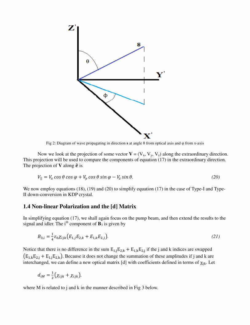
Fig 2: Diagram of wave propagating in direction s at angle θ from optical axis and φ from x-axis

Now we look at the projection of some vector V = (Vx, Vy, Vz) along the extraordinary direction.

This projection will be used to compare the components of equation (17) in the extraordinary direction.

The projection of V along ]2 is

|| � ^ /V& Y /V& W � a /V& Y &5X W b &5X Y. (20)

We now employ equations (18), (19) and (20) to simplify equation (17) in the case of Type-I and Type-

II down-conversion in KDP crystal.

1.4 Non-linear Polarization and the [d] Matrix

In simplifying equation (17), we shall again focus on the pump beam, and then extend the results to the

signal and idler. The ith

component of B3 is given by

P�,* � �Q !"B*CD;E�,CE�,D � E�,DE�,C<. (21)

Notice that there is no difference in the sum E�,HE�,I � E�,IE�,H if the j and k indices are swapped ;E�,IE�,H � E�,HE�,I<. Because it does not change the summation of these amplitudes if j and k are

interchanged, we can define a new optical matrix [d] with coefficients defined in terms of χijk. Let

c*d � �� ;B*CD � B*CD<,

where M is related to j and k in the manner described in Fig 3 below.

jk xx yy zz yz or zy xz or zx xy or yx

M 1 2 3 4 5 6 Fig 3: Prescription for defining index values of the matrix [d].

For the [d] matrix, index i is also typically written as 1, 2, or 3. Note that when j = k, diM = χijk. This

new optical matrix [d] has dimensions 3x6 and takes the place of the 3x3x3 χ tensor, which allows us to

write the B3 in a contracted 2-dimensional matrix notation.

�� 12 !0 fc11 c12 c13c21 c22 c23c31 c32 c33 c14 c15 c16c24 c25 c26c34 c35 c36

jklllllm E1,�E2,�E1,nE2,nE1,oE2,oE1,nE2,o � E1,oE2,nE1,oE2,� � E1,�E2,oE1,�E2,n � E1,nE2,�pq

qqqqr . (22)

Each non-linear crystal has different values of diM based upon their chemical and geometrical structures.

KDP crystals are tetragonal7 crystals of the 42m space group.

4 The optical tensor for KDP in contracted

notation is given by expression (21) below.4

s0 0 00 0 00 0 0 c�Q 0 00 c�Q 00 0 c�tu . (23)

From here, the final form of equation (17) depends upon whether we are studying Type-I or Type-II

down-conversion. We shall first focus on Type-I down-conversion, where both the signal and idler

photons are ordinary waves and the pump is an extraordinary wave. We shall deal with Type-II

afterwards.

Because both the signal and idler are ordinary, E1 and E2 both point in the ordinary direction,

and therefore their components will be determined by equation (18).

E�,` � E� &5X W

E�,` � E� &5X W

E�,a � E� /V& W

E�,a � E� /V& W

E�,b � 0

E�,b � 0.

Using the optical [d] matrix for the KDP crystal (23), expression (22) allows us to calculate the

individual components of B3.

B�,w � 0 (24a)

B�,x � 0 (24b)

B�,y � 12 ε"E1E2d�t sin 2φ. (24c)

The projection of B3 onto the extraordinary direction ]2, according to equation (20), is therefore

P�,|| � 12 !"E1E2c�t &5X 2W &5X Y. (25)

Expression (25) gives us the extraordinary component of B3. This completes the right side of equation

(17) for Type-I down-conversion where n=3. We now focus on A3.

1.5 Coupled Equations for Type-I and Type-II SPDC

A3 is given by

�� 9 k��>� � �� >� � 2ik�,� �� >� i 9�� ⋅ �� >�: �2 � (�� ⋅ >�)�� µεω��>�:. (26)

Firstly, k2 = µεω

2 in matter, so the first and final terms of (26) cancel out. We also make the

approximation that the amplitude E3 varies slowly over s, so that the second derivative terms is dwarfed

by the first derivative terms, and vanishes.

� ��6� E�� « �254�,6 776 E��.

Next, we project (26) onto the extraordinary direction. The term in the 12 direction immediately

vanishes because ]2 and 12 are orthogonal, while any terms in the E3 direction remain unchanged in

magnitude because the pump is assumed to be an extraordinary wave. Given these assumptions, (26)

now takes the form

��,|| � 254�,6 776 E� � 4�,��E� . (27)

Finally, we use the fact that the angle between E3 and D3 (the same angle between k3 and 12) is very

small for KDP (see Appendix), and also make a low-power approximation for E3, so that the second

term of expression (27) becomes much smaller than the first and vanishes. Therefore,

��,|| � 254�,6 776 E�. (28)

Now replace equation (28) and (25) into equation (17) and solve in terms of E3 to attain

776 E� � 54 �.0��D0,� E1E2c�t &5X 2W &5X Y. (29)

If we start again at Section 1.3 with

P�,* � �Q !"B*CD;E�,CE�,DR � E�,DE�,CR<,

in place of equation (21) and

=� � �� 9 4�� 6� �� 254�,6 776 �� 5 9�� ⋅ 776 ��: 12 � (�� ⋅ ��)�� !��:,

in place of equation (26), while repeating the same steps, we attain an equation analogous to (29):

776 E� � 54 �.+��D+,� E3E2Rc�t &5X 2W &5X Y. (30)

Finally, we follow the same steps with

P�,* � �Q !"B*CD;E�,CE�,DR � E�,DE�,CR<,

in place of equation (21) and

=� � �� 9 4�� 6� �� 254�,6 776 �� 5 9�� ⋅ 776 ��: 12 � (�� ⋅ ��)�� !��:,

in place of (26) to achieve a third equation:

776 E� � 54 �.��D0,� E3E1Rc�t &5X 2W &5X Y. (31)

Equations (29), (30), and (31) show the coupled nature of the three plane waves involved in Type-I

down-conversion from a KDP crystal. Similar equations are found in several textbooks on the subject

of non-linear optics.4, 8, 9

Type-II down-conversion has similar coupled equations. The difference is that one of the

outgoing photons is an extraordinary wave. To find the coupled equations for Type-II SPDC, the

components of the electric fields in the matrix equation (22) are determined by using equation (18) for

one of the waves, say E1, and equation (19) for the other, say E2.

E�,` � E� &5X W

E�,` � E� /V& Y /V& W

E�,a � E� /V& W

E�,a � E� /V& Y &5X W

E�,b � 0

E�,b � E� &5X Y.

Using these components and matrix (23) in equation (22), the components of B3 for Type-II are

P�,` � 12 !0E1E2c�Q /V& W &5X Y (32a)

P�,a � 12 !0E1E2c�Q &5X W &5X Y (32b)

P�,a � 12 !0E1E2c�t /V& Y (&5X W� /V& W�). (32c)

To take the projection of B3 along ]2, replace (32) into equation (20).

P�,|| � �� !"E1E2(c�Q � c�t)(/V& W� &5X W�) &5X Y /V& Y. (33)

From equation (33), the derivation is identical to Type-I. The coupled equations for Type-II SPDC are

776 E� � *Q �.0��D0,� E�E�(c�Q � c�t)(/V& W� &5X W�) &5X Y /V& Y (34)

776 E� � *Q �.+��D+,� E�E�R(c�Q � c�t)(/V& W� &5X W�) &5X Y /V& Y (35)

776 E� � *Q �.��D�,� E�E�R(c�Q � c�t)(/V& W� &5X W�) &5X Y /V& Y. (36)

The only difference between the Type-I coupled equations (29), (30), and (31) and the Type-II coupled

equations (34), (35), and (36) is the last constant containing components of the [d] matrix and polar

coordinates. These factors can be condensed into a single constant, deff. For Type-I SPDC,

c�� c�t &5X 2W &5X Y.

For Type-II,

c�� (c�Q � c�t)(/V& W� &5X W�) &5X Y /V& Y.

2.1 Polarization Entanglement for Type-I and Type-II SPDC

Now that a theory has been developed for the creation of polarization-correlated photons using

a single frequency laser (the pump) and a uniaxial crystal, we analyze entanglement of the polarization

states of the signal and idler. This chapter will describe methods for attaining polarization entanglement

for both Type-I and Type-II SPDC.

Quantum mechanics is a fundamentally statistical theory. This means that it does not attempt to

predict what will happen, only the probabilities of certain events. Mathematically, a system that could

be in one of multiple states is represented as a linear combination of those states. For example, if the

polarization of a photon is going to be measured, and can either be polarized horizontally or vertically,

the state of the photon, �, is given by

|�� |�� |�^��,

where a and b are complex numbers which give weight to |��, the horizontal state, and |�^��, the

vertical state, based upon their probabilities, such that |a|2+|b|

2=1. The photon is said to be in a

superposition of horizontal and vertical polarization if neither a nor b is equal to zero.

Quantum entanglement between two particles occurs when the particles are in a quantum

superposition of states, and their states are correlated. Both types of SPDC have correlated photon

polarization. In Type-II down-conversion, photons can be found in a superposition of polarization states

where the signal and idler cones intersect (Fig 4). On one cone lie extraordinarily polarized rays, while

the other has ordinary rays. At the intersection points, it cannot be determined from which cone a

photon originated, and therefore it cannot be determined what the polarization of a photon is before a

measurement is taken. This means a photon at an intersection point is in a superposition of ordinary and

extraordinary (or horizontal and vertical) polarization states. Because the photons produced also have

correlated polarizations, the photons found at the intersection points are entangled. The state of this

system is given by

�|�� |�� |^�� |^�� |��, (37)

Fig 4: Type-II entangled photons from SPDC crystal

photon exists on the other cone with vertical polarization. This is correlation. When a photon exists on an intersection poin

it cannot be said from which cone it came from, and it is thu

correlation and superposition leads to entanglement.

where subscripts A and B refer to photon A and photon B.

In Type-I SPDC, the signal and idler are both ordinarily

polarizations are correlated, neither are in a superposition of states.

produced from Type-I down-conversion, but it requires the use of two crystals with identical optical

axes. When the crystals are placed back to back

about the direction of pump propagation

a basis, the pump will be seen as being in a superposition of ordinary and extraordinary polari

until it interacts with one of the crystals.

extraordinary pump. As long as the pump beam was

it will be unknown through which crystal the pump

must be thin enough so that the cones cannot be distinguished at the detection

mm. For more on the effects of crystal length on down

If two photons, A and B, are

basis of horizontal polarization |H� and vertical polarization written as

An entangled state is said to be

by coefficient a is just as likely to be measured as the state weighted by coefficient

entangled pair is called a Bell state. For Type

incoming photon to have polarization at a 45

entangled photons are always produced in a Bell state in Type

will always have opposite polarizations.

II entangled photons from SPDC crystal. When a photon from one cone has horizontal polarization, another

photon exists on the other cone with vertical polarization. This is correlation. When a photon exists on an intersection poin

it cannot be said from which cone it came from, and it is thus in a superposition of polarization states.

correlation and superposition leads to entanglement.

where subscripts A and B refer to photon A and photon B.

, the signal and idler are both ordinarily polarized, so although t

polarizations are correlated, neither are in a superposition of states. Entangled photons

conversion, but it requires the use of two crystals with identical optical

axes. When the crystals are placed back to back, their axes must be orientated such that one is rotated

about the direction of pump propagation by 90° from the other. Using the two crystal axis directions as

a basis, the pump will be seen as being in a superposition of ordinary and extraordinary polari

until it interacts with one of the crystals. SPDC may occur if one of the crystals “observes” an

s long as the pump beam was not polarized exactly along one of the crystal axes,

it will be unknown through which crystal the pump beam was down-converted (see Fig 5

must be thin enough so that the cones cannot be distinguished at the detection zone, usually about 1

. For more on the effects of crystal length on down-conversion, see Ramirez et. al.

A and B, are entangled through Type-I down-conversion and measured in the and vertical polarization |V�, then the state of the system is .

state is said to be maximally entangled if a = b. In this case,

is just as likely to be measured as the state weighted by coefficient b

entangled pair is called a Bell state. For Type-I entanglement, this can be achieved by setting the

incoming photon to have polarization at a 45° angle relative to both crystal axes. Polarizations

entangled photons are always produced in a Bell state in Type-II SPDC because the signal and idler

e polarizations.

. When a photon from one cone has horizontal polarization, another

photon exists on the other cone with vertical polarization. This is correlation. When a photon exists on an intersection point,

s in a superposition of polarization states. The combination of

, so although their

photons can still be

conversion, but it requires the use of two crystals with identical optical

, their axes must be orientated such that one is rotated

Using the two crystal axis directions as

a basis, the pump will be seen as being in a superposition of ordinary and extraordinary polarizations

if one of the crystals “observes” an

along one of the crystal axes,

see Fig 5). The crystals

, usually about 1

conversion, see Ramirez et. al.10

conversion and measured in the , then the state of the system is (38)

the state weighted

b. This maximally

this can be achieved by setting the

angle relative to both crystal axes. Polarizations

II SPDC because the signal and idler

Fig 5: Type-I entangled photons from two

the pump propagation direction from the 1

ordinarily polarized relative to the 1st crystal axis. I

correlation. The cones are too close together to determine from which

superposition of polarization states. Entangled pairs can be found at any points

The four Bell states for a pair of photon entangled particles

The states are only possible from T

from Type-II down-conversion. Bell states are typically preferable in entanglement experiments

possible results of a measurement are equally likely to occur.

2.2 Bell Inequality and Local

Entanglement, like the superposition of states, is a quantum mechanical effect that is completely

foreign to our classical intuition. For example

of a spin-0 particle, they will have opposite spins

results of these measurements will always be opposites. This means that if the spin of the

measured, the result of a similar spin measurement on the positron will be immediately known to the

observer, even if the positron has yet to be measured.

Quantum effects are known to break fundamental assumptions we make about

universe. One such assumption is known as realism, which is the idea that particles exist in definite

states before being observed. In other words, if a tree falls in a forest and no one is around to hear it, a

realist would say that it does make a sou

information can be transmitted faster than the speed of light (locality), though this idea is backed by

much observation. Together, these ideas are known as local

from two identical uniaxial crystals. The crystal axis of the 2nd

crystal is rotated 90

the pump propagation direction from the 1st crystal axis. If SPDC occurs in crystal #1, both outgoing

crystal axis. If SPDC occurs in crystal #2, they will be ordinary to the 2

The cones are too close together to determine from which crystal the photons originate, so they

superposition of polarization states. Entangled pairs can be found at any points around the cone, opposite

four Bell states for a pair of photon entangled particles are

.

states are only possible from Type-I down-conversion, while the states are only possible

Bell states are typically preferable in entanglement experiments

possible results of a measurement are equally likely to occur.

Local-realism


. For example, when an electron-positron pair is created

have opposite spins. When their spins are measured in the same basis, the

results of these measurements will always be opposites. This means that if the spin of the


observer, even if the positron has yet to be measured.

Quantum effects are known to break fundamental assumptions we make about

One such assumption is known as realism, which is the idea that particles exist in definite


make a sound. Another idea we hold about the universe is that no


much observation. Together, these ideas are known as local-realism. Superposition of states and

crystal is rotated 90° about

outgoing photons will be

be ordinary to the 2nd

axis. This is

crystal the photons originate, so they are in a

, opposite each other.

states are only possible

Bell states are typically preferable in entanglement experiments, as all


positron pair is created from the decay

. When their spins are measured in the same basis, the

results of these measurements will always be opposites. This means that if the spin of the electron is


Quantum effects are known to break fundamental assumptions we make about the nature of the

One such assumption is known as realism, which is the idea that particles exist in definite


nd. Another idea we hold about the universe is that no


uperposition of states and

entanglement, which are not part of our classical world view, create problems for us under these

assumptions.

For some time, the apparent randomness of quantum mechanics was thought to be due to

unknown effects that were not taken into account by quantum theory. The Bell Inequality was the first

rigorous mathematical theory to both challenge our perception of local-realism and hidden variables in

a testable and predictable manner. Bell’s theorem invoked the use of expectation values.

When photons are produced via Type-II down-conversion, they are always measured to have

opposite polarization when measured using similarly oriented polarizers. If there is a local hidden

variable, say §, which hides a deterministic explanation of quantum theory, then there must be

functions of § and polarizer direction which give the polarizations of photons A and B. Let these

functions be defined as �(�, §) and P;�© , §< respectively. Let horizontal polarization be given a value of

+1, and vertical polarization be given -1. Therefore, these functions are limited to:

�(�, §) � ª1 (38a)

and P;�© , §< � ª1. (38b)

Because these photons always have opposite polarization, if they are measured in the same direction �,

�(�, §) � P(�, §). (39)

If p;�, �© < is the expectation value of the products of �(�, §) and P;�© , §<, then

«;�, �© < � ¬ (§)�(�, §) P;�© , §<c§, (40)

where (§) is the probability density for the hidden variable, supposing it exists. Using equation (39), P;�© , §< can be replaced with �;�© , §<. If we introduce another polarizer direction using the unit vector /, we can find a difference value between two different expectation values.

«;�, �© < «(�, /) � ¬ (§)®�(�, §)�;�© , §< �(�, §)�(/, §)¯c§. (41)

Given that the hidden variable function can only result in we see ª1 for any polarizer direction, we see

that ®�;�© , §<¯� � 1. Therefore we are safe to multiply by ®�;�© , §<¯� without changing any values.

«;�, �© < «(�, /) � ¬ (§)®�(�, §)�;�© , §< �(�, §)�(/, §)¯®�;�© , §<¯�c§. (42)

We can now rearrange equation (42) by factoring out �(�, §) and distributing �;�© , §<.

«;�, �© < «(�, /) � ¬ (§)®1 �;�© , §<�(/, §)¯�(�, §)�;�© , §<c§. (43)

From equation (38a), we see that �(�, §)�;�© , §< � ª1. This is also true of �;�© , §<�(/, §). Because (§) is a positive number, it is also true that (§)®1 �;�© , §<�(/, §)¯ ° 0. Therefore, if we take the

absolute value of p;�, �© < p(�, /),

±«;�, �© < «(�, /)± ² ¬ (§)®1 �;�© , §<�(/, §)¯c§. (44)

Substituting P(/, §) for �(/, §), and taking the integration in equation (44), we end up with the Bell

Inequality.

± «;�, �© < «(�, /)± ² 1 � «(�© , /). (45)

This inequality was developed in this form in 196411

by J.S. Bell under the assumptions that the

hidden variable was local (in that information does not travel faster than light) and that the measurable

quantities exist regardless of whether or not a measurement was taken (realism). A violation of this

inequality is therefore a violation of one or both of these assumptions. The same exact inequality can be

derived for Type-I down-conversion as well. The only difference in the derivation is that in Type-I,

polarizations are always the same if measured in the same way, so equation (39) becomes �(�, §) �P(�, §).

After the development of equation (45), a more intuitive formulation was built by Hardy12

upon

the same basic assumptions. Instead of using the expectation value of the product of the measurement

results, Hardy simply used the probabilities of various states.

The state of a photon of unknown polarization can be written as a function of the angle θ

relative to the horizontal direction.

�|Y� � /V& Y �|�� &5X Y �|^�. (46)

The probability to detect photons entangled by Type-I down-conversion in state (θAi ,θBj) can now be

found. By taking the squared absolute value of the dot product of the initial entangled state Eq(3) with

the final state A⟨θi| B⟨θj|, the probability is found to be

A;Y�* , Y�C< � ± ⟨Y�* �|�µY�C �|� � |�� ±� � ±(/V& Y�* ⟨��|� &5X Y�* ⟨^�|);/V& Y�C ⟨��±� &5X Y�C ⟨^�±<(��|�� |�� |^�� |^��)±�

(57)

Simplifying equation (57) we attain

A;Y�* , Y�C< � ±� /V& Y�* /V& Y�C � � &5X Y�* &5X Y�C±�. (58)

Hardys Inequality entangled photons is

A(Y�� , Y��) ° A(Y�� , Y��) A(Y�� ª 90° , Y��) A(Y�� , Y�� ª 90°). (59)

Though the Hardy Test can be used for any general quantum entanglement, in this paper, we apply it

only to down-conversion and polarization states. This expression is derived more rigorously by

Mermin13

. Expression (59) inhibits P(θA2 ,θB2) from going below a certain threshold if local-realism is

to stand. Each individual term of this inequality is experimentally determined using the number of

coincident detections of photons in state (θAi ,θBj), given by N(θAi ,θBj).

A;Y�* , Y�C< � $;\·¸ ,\¹º<$;\·¸ ,\¹º<»$;\·¸ª¼"° ,\¹º<»$;\·¸ ,\¹ºª¼"°<»$;\·¸ª¼"° ,\¹ºª¼"°< . (60)

In order to better understand the Hardys inequality, consider this thought experiment. Imagine a

single photon source that produces pairs of entangled photons that are sent in different directions, such

as a down-conversion crystal. One photon goes to detector A, and is observed by Alice, while the other

goes to B and is observed by Bob. Before reaching their respective detector, the photons must pass

through a respective polarizer. Polarizer A is oriented arbitrarily to either angle θA1 or θA2 just after the

photons are produced and just before measurement. Polarizer B is similarly randomly oriented to either

θB1 or θB2. This constraint is to make sure no information about one polarizer has time to reach the

other before a measurement is taken.

In this experiment, the probability for both Alice to detect a photon with polarization θAi and

Bob to detect a photon with polarization θBj is P(θAi ,θBj). The probability of Alice to detect a photon

with polarization θA1 given Bob detected a photon at θBj is P(θAi | θBj).

After many trials are run, assume that Alice and Bob exchange and compare their data, and the

following observations are made:

1 If detector A is set to θA1 and detector B is set to θB1, there is a nonzero probability for both

Alice and Bob to detect a photon at their counter. A(Y�� , Y��) ½ 0

2 Given that Bob has detected a photon with polarizer θB1, Alice always detects a photon at

angle θA2 A(Y��|Y��) � 1

3 Given that Alice has detected a photon with polarizer θA1, Bob always detects a photon at

angle θB2 A(Y��|Y��) � 1

Applying our classical logic to these three observation, we can extrapolate what should logically be

observed regarding P(θA2 ,θB2). As stated before, we shall assume that polarization states exist

regardless of being measured. Given observation 2 and 3, whenever Bob detects a photon with

polarization θB1 and Alice detects a photon with polarization θA1, had they instead chosen to orientate

their polarizers at θB2 and θA2, they would be at least as likely to detect a photon at those positions as

well.

A(Y�� , Y��) ° A(Y�� , Y��). (61)

This relationship does not take into account the probabilistic nature of the measurements. It could be

that P(θA2 | θB1) and P(θB2 | θA1) are slightly less than 1, but the coincidental measurements simply

happened to be made every time. We account for this possibility by restating observations 2 and 3 in a

logically equivalent manner and then examining the effect of experimental error. According to

observation 2, if Bob’s photon is found polarized along θB1, then Alice always find her photon with

polarization θA2. This means that it would never be the case that Alice finds her photon along θA2 ± 90°

and Bob finds his along θB1.

A(Y��|Y��) � 1 ¾ A(Y�� ª 90° , Y��) � 0.

Similarly, according to observation 3, Bob will never find his photon along θB2 ± 90° if Alice’s is along

θA1.

A(Y��|Y��) � 1 ¾ A(Y�� , Y�� ª 90°) � 0.

We must recognize that it is impossible to experimentally prove that any event has zero

likelihood. Any seemingly impossible event may not occur after millions of trials, and yet it may occur

on the next run. If P(θA2 ± 90° ,θB1) and P(θA1 , θB2 ± 90°) was nonzero, say 0.01 each, then there would

be a reduction of 0.02 from P(θA2 ,θB2). Given this possibility, expression (61) must be modified.

This is the Hardy inequality from expression (59

experimental data, assume that Alice and Bob compare notes regarding

the two measurements never coincide.

.

This result would lead to a violation of the Hardy inequality

classical intuition. Indeed, real world examples of a violation of

down-conversion and other quantum entanglement phenomena.

3.1 Quantum Teleportation using Entangled P

It has long been established that any measurement of a particle in a superposition of states

replaces the probability distribution with a definitive state.

principle, we also know that it is also impossible to know all quantities related to a particle

simultaneously. Given these facts, it seems impossible to scan a group of particles, and reconstruct

them exactly as they were in another location.

teleportation is impossible, but the answer to this problem is found in entanglement.

We start with a source of polarization entangled photons A and B.

Type-I down-conversion, so that they will

using similarly oriented polarizers. Make sure that the entangled pair is in a Bell state, so that the

photons are just as likely to be horizontally or vertically polarized relative to the pump.

another photon (let’s call it photon X) with photon A and measuring the type of entanglement that A

and X share, we can then send that information to B through a classical signal

has the same polarization as X, all without e

Fig 6: Basic diagram for quantum teleportation of photon X. Photons A and B are entangled, usually through SPDC, and

then photons A and X are also entangled. Information about the nature of the entanglement is sent to photon

.

from expression (59). Finally, after calculating each probability using their

Alice and Bob compare notes regarding θA2 and θB2, and they find that

the two measurements never coincide.

to a violation of the Hardy inequality, which would mean a violation of our

classical intuition. Indeed, real world examples of a violation of expression (59) have been verified for

conversion and other quantum entanglement phenomena.14

tum Teleportation using Entangled Photons


replaces the probability distribution with a definitive state. Based upon the Heisenberg uncertainty

know that it is also impossible to know all quantities related to a particle


them exactly as they were in another location. This makes it seem that even non-instantaneous

he answer to this problem is found in entanglement.

We start with a source of polarization entangled photons A and B. Let them be entangled by

conversion, so that they will either both be horizontal or both be vertical when

Make sure that the entangled pair is in a Bell state, so that the

photons are just as likely to be horizontally or vertically polarized relative to the pump.

photon (let’s call it photon X) with photon A and measuring the type of entanglement that A

and X share, we can then send that information to B through a classical signal and change B so that it

has the same polarization as X, all without ever knowing their polarizations (see Fig 6

: Basic diagram for quantum teleportation of photon X. Photons A and B are entangled, usually through SPDC, and

then photons A and X are also entangled. Information about the nature of the entanglement is sent to photon

fter calculating each probability using their

, and they find that

, which would mean a violation of our

) have been verified for


Based upon the Heisenberg uncertainty

know that it is also impossible to know all quantities related to a particle


instantaneous

he answer to this problem is found in entanglement.

Let them be entangled by

ntal or both be vertical when measured

Make sure that the entangled pair is in a Bell state, so that the

photons are just as likely to be horizontally or vertically polarized relative to the pump. By entangling

photon (let’s call it photon X) with photon A and measuring the type of entanglement that A

and change B so that it

r polarizations (see Fig 6).

: Basic diagram for quantum teleportation of photon X. Photons A and B are entangled, usually through SPDC, and

then photons A and X are also entangled. Information about the nature of the entanglement is sent to photon B.

The method of entangling photons A and X can be very difficult, and requires careful timing

and precision. In general however, A and X can interact with a polarizing beam splitter simultaneously,

and through that interaction become entangled in their polarization (see Fig 7). Following the beam

splitter, two detectors can be placed in the paths of the photons (see Fig 8). If photons A and X have are

polarized such that their polarizations will always be measured as orthogonal, then both detectors will

click. If the photons are entangled such that they have the same polarization, only one of the detectors

will click. Photon X could be produced using the same crystals to make sure that their polarizations are

always either aligned or orthogonal. This shows that different Bell states can produce different effects.

If two clicks are detected, rotating B by 90° with a polarization rotating crystal that can be

controlled externally will make B have the same polarization as X. Likewise, if one click is detected, B

is already the same as X. Although photons A and X must be destroyed in this process, the quantum

state of X is transferred to B without ever having to measure it in a way that would give us unique

information of its polarization. All that is measured is which kind of entanglement is shared between

photons A and X. This information would have to be sent through the classical channel before photon B

reached its destination. Information through the classical channel cannot travel faster than light, so

photon B must be delayed in some way. This could be achieved by lengthening its path using mirrors,

or by sending it through a medium which significantly slows its speed. Quantum teleportation could

also be achieved through Type-II down-conversion if B is kept unchanged when two clicks are detected,

and instead rotate B if one click is detected.

Fig 7: Entangled photons interacting with a polarizing beam splitter simultaneously. TOP: When two photons are entangled

such that they always have the same polarization, their probability waves will interfere such that they will only be detected

on the same side of the beam splitter after interacting with it. BOTTOM: When polarized orthogonally, the photons will

always exit on opposite sides of the beam splitter. It is impossible to tell whether they were reflected or if they passed

through.

Fig 8: Photons A and X are sent to a beam splitter si

be detected by either Detector 1, Detector 2, or both depending upon the entanglement relationship between the two photons.

The result will not tell us the state of either photon, but i

3.2 Entanglement Transfer from

Now let us examine what happens when photon X is entangled with another photon before

being entangled with photon A. If X is

was done in section 3.1, then the information of photon X will be transferred to photon B. However, if

X is entangled with photon Y, as in Fig 9, the only information that is know

superposition of polarization states and is correlated to Y.

transferred to B. Similarly, the only information known about A is that it is entangled with B, therefore

that information is transferred to Y. The result is that photons B and Y are

interaction with each other, but through the interactions of A and X. This phenomenon is called

entanglement transfer.1

Fig 9: Diagram for entanglement transfer from photons A and X to photons B and Y. Photons A and B are initi

entangled, as are photons Y and X. Photons A and X are then entangled. Information about the nature of the entanglement is

: Photons A and X are sent to a beam splitter simultaneously and are entangled once exiting. The outgoing photons will


The result will not tell us the state of either photon, but it will give us the entanglement state.

from Photons to Matter


being entangled with photon A. If X is entangled with A without measuring their individual states, as


X is entangled with photon Y, as in Fig 9, the only information that is known about X is that it is in

n states and is correlated to Y. That is exactly the information that


The result is that photons B and Y are now entangled, not through


Diagram for entanglement transfer from photons A and X to photons B and Y. Photons A and B are initi


transferred to photons B and Y.

multaneously and are entangled once exiting. The outgoing photons will


t will give us the entanglement state.


individual states, as


about X is that it is in

t is exactly the information that is


now entangled, not through


Diagram for entanglement transfer from photons A and X to photons B and Y. Photons A and B are initially


Entanglement transfer need not occur exclusively between photons. It has been observed that

entangled photons can interact with plasmons on periodically perforated metal plates, be reradiated on

the other side of their respective plates, and still retain their entanglement (see Fig 10).15

Plasmons are

localized electromagnetic waves formed at a dielectric-metal interface, which are stimulated by

interactions with light, usually heavily dependent on frequency. The propagation of plasmons are

associated with the collective motion of a large number of electrons. The perforations on the metal

plates are periodically spaced and smaller than the wavelength of the incident light, which leads to a

very efficient light transmission where light tunnels through each sub-wavelength aperture. This is an

indication of a cooperative effect where incident photons are scattered off the periodic arrangement of

holes and converted into a surface-plasmon. In the case of plasmons incidnt down-converted photons,

we expect them to pass through the holes to reradiate on the other side of the plate. If an incoming

photon is horizontally polarized, the electron wave will transfer energy horizontally across the metal

through horizontal oscillations. When the plasmons pass through the perforated surface, the direction of

oscillation remains the same. Finally, when the plasmons reradiate another photon, these horizontal

oscillations in the material will produce a horizontally polarized photon. Because entanglement can

easily be destroyed through interactions, and given the collective nature of the surface plasmons, which

involves large numbers of electrons, it seems remarkable that entanglement survives. It can be inferred

that the plasmons on the metal plates retained the entanglement during transition from light to matter.

The entanglement is transferred because the direction of polarization for either individual photon is

unknown, so it is unknown which plate is experiencing horizontal oscillations, and which is

experiencing vertical oscillations.

One application for entanglement has been in quantum computing, where the classical two-state

bit is replaced with the qubit, which can be in multiple states simultaneously. By entangling multiple

qubits, quantum computers are theorized to be able to excel in parallel computing where classical

computers cannot compare. The main limitation has been in both creating many entangled states and

storing them so that their entanglement is stable. While it is easy to entangle a number of photons, it is

very difficult to store them for future use. Also, while even single particles can be contained and

arranged, such as charged particles within ion traps16

, it can be difficult to arrange and manipulate them

after they have been entangled. Transferring entanglement from light to matter could potentially ease

these difficulties, as it combines the simplicity of entangling photons with SPDC with the ease of

storage of particles.

Fig 10: Schematic for photon-to-plasmon entanglement transfer. Down-converted photons stimulate plasmons on

metal plates with regular perforations. Reradiated photons pass through identical polarizers then to photon detectors. The

entanglement is verified using the coincidence counter.

Conclusion

A theory of spontaneous parametric down-conversion has been presented using Maxwell’s

equations to describe electromagnetic wave propagation in quadratic non-linear uniaxial crystals. It has

been shown that through SPDC, quantum entanglement can be achieved via a process that is simple to

implement in a lab and can be understood using classical theory. The polarization entanglement of

photons through SPDC has been shown to violate the Bell and Hardy inequalities, and throw local-

realism into doubt. The simple SPDC methods for entanglement gives way to the possibility that light

to matter entanglement transfer is the preferable method in creating stable and easily containable multi-

particle entangled states, and thus simplifying the production of quantum computers. In general, it is

difficult to localize and store photons, so usually one prefers choosing matter as quantum memory

elements. The interface between quantum carrier and memory is a key component in the realization of

scalable quantum networks. A scheme has been proposed to transfer entanglement from photons to

nano-scale resonators constructed from movable mirror cavities, which oscillate at frequencies

dependent upon the radiation pressure within the cavity when at cryogenic temperatures17

. Each of the

down-converted photons is absorbed into one of the mirror cavities (see Fig 11). This setup takes

advantage of the superposition of frequency states of the signal and idler photons, so it is unknown

which nanoresonator has absorbed ��, and which has absorbed ��.This causes the nanoresonators to

be in a superposition of oscillation modes and be correlated with each other, and therefore be entangled.

The quantum computing industry could benefit from producing and transferring entanglement

from light to matter using the relatively simple process of spontaneous parametric down-conversion.

Further research is required to determine how to best utilize plasmons for quantum computing. Photons

are the fastest carriers of quantum information for transmission, and the transmission of that

information to matter could circumvent difficulties in localizing and storing photons for manipulation

in quantum computers.

Fig 11: Two down-converted photons are each sent to and absorbed by a nanoresonating mirror cavity, which oscillate upon

absorption. The mode of oscillation depends upon the energy (frequency) of the absorbed light. The two photons have

frequencies that are related by �� , but it is unknown which photon is of frequency ��, and which is of ��.

Therefore, the mirror cavities M1 and M2 are entangled in their modes of oscillation.

Acknowledgements

I give thanks to my advisor, Dr. La Rosa, for his guidance and supervision on this piece for the

past year. His dedicated support, time, and resources have been a major factor in the completion of this

thesis. I would also like to thank Mark Beck for providing insight into the nature of entanglement.

Appendix – Vector Orientation Relative to the Principle Axis

In the most general case, E and D in a non-linear material can be related by

¿C � ∑ εHGEG* , where j,i = 1,2,3.

However, in the principle axis reference frame, the relationship can be written using the principal

dielectric permittivities,

� � ;εwEw , εxEx , εyEy <.

In this frame, E and D are always parallel when along the x, y, and z directions. In a uniaxial medium

such as a KDP crystal (KH2PO4), where εw � εx À εy, the z-axis has a different index of refraction

from the other two axes. Therefore, the behavior of light within a uniaxial medium will depend upon

whether or not its polarization has a z-component. Because of this, the z-axis is often referred to as the

extraordinary axis or optical axis. The indices are also given special names:

X� � ÁÂÃÂ� � ÁÂÄÂ� Ordinary refractive index

X� � ÁÂÅÂ� Extraordinary refractive index

Let E and D be plane waves described by

�(,, () � �")*(�⋅,-ÆÇ) (A-1)

�(,, () � �")*(�⋅,-ÆÇ), (A-2)

where Eo and Do are constants, k is the wave vector, and ω is the frequency. Replacing (A-1) and (A-2)

into equation (4) results in

� x (� x �) � µω��,

which shows that D and k are perpendicular, and that E lies in the same plane as D and k. If E and D

lie in the xz-plane, then

¿` � εwEw � ε"X��E` (A-3)

¿b � εyEy � ε"X��Eb. (A-4)

Figure A-1: Several vectors of an extraordinary wave in the principle axis reference frame. Angle ϕ is between E and D,

and θ is between k and z.

If E is an angle ϕ from D, and k is an angle θ from the optical axis as in Fig A-1, then

ÈÉÈÊ � tan θ (A-5)

ÌÉÌÊ � tan(θ � Í). (A-6)

Replacing (A-3) and (A-4) into (A-5),

ÌÉÌÊ � KÎ�

KÏ� tan θ. (A-7)

Replacing (A-6) into (A-7), after some algebra, results in

Í � tan-� 9KÎ�KÏ� tan θ: θ. (A-8)

The values of the ordinary and extraordinary refractive indices can be calculated from the Sellmeier

equations for KDP crystal (Kwiat, pg. 17)18

,

X�� 2.259276 � "."�""Ñ¼ÒtÓ�-"."��¼Q�t�Ò � Ó��.""Ò��Ó�-Q"" (A-9)

X�� 2.132668 � ".""Ñt�ÕQ¼QÓ�-"."��Ñ�"Q� � Ó��.��Õ¼¼�QÓ�-Q"" , (A-10)

where § is the wavelength of light in micrometers. The ratio of the squares of the refractive indices

from (A-9) and (A-10) ranges from 1.05 to 1.06 when § is confined to the visible spectrum. In that case,

according to (A-8), the value of Í is very small in KDP, with a maximum of about 1.67 degrees or 0.03

radians. This result is used in section 1.5 to approximate that the component of k in the direction of E is

negligible when compared to the component of k in the direction of s.

References

1. A. Zeilinger, (2010). “Dance of the Photons: From Einstein to Quantum Teleportaion”. New

York: Straus and Giroux. Print.

2. A. Zavatta, S. Viciani, and M. Bellini, (2004). “Tomographic reconstruction of the single-

photon Fock state by high-frequency homodyne detection”. Phys. Rev. A 70, 053821.

3. M. Beck, (2012). “Quantum Mechanics: Theory and Experiment”. Oxford, New York: Oxford

University Press.

4. A. Yariv and P. Yeh, (2007). “Photonics: Optical Electronics in Modern Communications 6th

edition”. Oxford, New York: Oxford University Press.

5. J. B. Pors, (2011). “Entangling Light in High Dimensions”. Ph.D. thesis, Leiden University.

6. P.G. Kwiat, K. Mattle, H. Weinfurter, and A. Zeilinger, (1995). “New high-intensity source of

polarization-entangled photons”. Phys. Rev. A 75, 4337.

7. Y. Ono, T. Hikita, and T. Ikeda, (1987). "Phase Transitions in Mixed Crystal System K1-

x(NH4)xH2PO4". Journal of the Physics Society Japan 56 (2), 577. doi:10.1143/JPSJ.56.577.

8. F. Zernike and J.E. Midwinter, (1973). “Applied Nonlinear Optics”. John Wiley & Sons Inc.

9. R.W. Boyd, (1992). “Nonlinear Optics”. San Diego, CA: Academic Press Inc.

10. R. Ramirez-Alarcon, H. Cruz-Ramirez and A. B. U’Ren, (2013). “Effects of crystal length on

the angular spectrum of spontaneous parametric downconversion photon pairs”. Laser Phys.

DOI 23 :10.1088/1054-660X/23/5/055204.

11. B. John, (1964). "On the Einstein Podolsky Rosen Paradox". Physics 1 (3): 195–200.

12. L. Hardy, (1993). “Nonlocality for two particles without inequalities for almost all entangled

states”. Phys. Rev. Lett. 71, 1665.

13. N. D. Mermin, (1994). “Quantum mysteries refined”. Am. J. Phys. 62, 880.

14. J.A.Carlson, M.D. Olmstead, and M. Beck, (2006). “Quantum mysteries tested: An experiment

implementing Hardys test of local realism”, American Association of Physics Teachers DOI:

10.1119/1.2167764,

15. E. Altewischer, M.P. van Exter, and J.P. Woerdman, (2002). “Plasmon-assisted transmission of

entangled photons” Nature 418, 304.

16. D. Stick, W. K. Hensinger, S. Olmschenk, M. J. Madsen, K. Schwab and C. Monroe, (2006).

"Ion trap in a semiconductor chip". Nature Physics 2, 36-39.

17. J. Zhang, K. Peng, S. Braunstein, (2003). “Quantum-state transfer from light to macroscopic os-

cillators”. Phys. Rev. A 68, 013808.

18. P. G. Kwiat, (1993). “Nonclassical effects from spontaneous parametric down-conversion:

Advetures in quantum wonderland”. University of California, Berkely.

Documents

Spontaneous Parametric Down-Conversion and Quantum ... · Spontaneous Parametric Down-Conversion and Quantum Entanglement by Jesse Catalano An undergraduate honors thesis submitted