SPLINE TECHNIQUES FOR GENERATING AIRPLANE WINGSWITH PRACTICAL APPLICATIONS

Karl-Heinz BRAKHAGERWTH Aachen, Germany

ABSTRACT: In the present paper we describe the CAGD part of an effort that aimed at the unifi-cation of the whole geometric preprocessing that preceded the wind tunnel readings with a realisticair-plane wing model in a recent research project. This preprocessing includes the automated gener-ation of the CAD models which were used for the manufacturing of the multi-parted wing-fuselageconfiguration and the generation of the numerical grids for the corresponding numerical simulations.Due to the constraints of the project it was decided to employ only exact, watertight, untrimmed B-Spline representations. From this process we describe the methods and algorithms for automatedgeneration of multi-parted airplane wings from one or more cross-sections given by point cloudsand the top view of the wing. A rounded wing tip an several types of winglets can be added. Fur-thermore we can compute and add fuselages to achieve realistic results near the root of the airfoilwing.

Keywords: B-splines, CAGD, approximation, fairing.

. . . . . . . . . . . . . . . . . . . . . . . . . . . . . . . . . . . . . . . . . . . . . . . . . . . . . . . . . . . . . . . . . . . . . . . . . . . . . . . . . . . . . . . . . . .

1 INTRODUCTIONIn the Collaborative Research Center SFB 401,”Modulation of Flow and Fluid-Structure Inter-action at Airplane Wings”, the aerodynamics ofhigh lift and cruise configurations and the in-teraction of structural dynamics and aerodynam-ics are presently being investigated. In the sub-project ”High Reynolds Number Aero-StructuralDynamics” stationary and unsteady wind tunnelreadings with an elastic model have been car-ried out. The experiments were done in the Eu-ropean Transonic Wind-Tunnel (ETW) in De-cember 2006. The wing corresponds to a cruiseconfiguration of scale 1:28, whose supercriticalcross-section (BAC 3-11) is described in twoAGARD reports ([9]). The geometry of the BAC3-11 aerofoil cross-section was numerically de-fined and the design ordinates were provided.The tolerances on the profile were given. Theairfoil is modeled as a three parted back-sweptwing with a rounded tip. To achieve realisticresults a half-body is placed between the air-foil wing and the wind tunnel wall. For a fu-

ture transfer project we are currently working onairfoils with winglets. The developed tools arebased on B-spline representations. Approxima-tion and fairing methods have to fulfill severalconstraints. These depend upon the manufactur-ing and the phenomena of adaptive flow solversfor the Navier-Stokes equations. It turned outthat especially for numerical simulation fairingof the geometry is very important . We use a fi-nite volume method as flow solver. Adaptationand error estimation is based on a multi-scaleanalysis.In this article we describe some details on meth-ods and algorithms for the automated genera-tion of multi-parted airplane wings from one ormore cross-sections given by point clouds andthe top view of the wing with the following prop-erties. The relative thickness of the wing (thick-ness/chord) can be varied from section to section.A rounded tip with design parameters and GC1-continuity at the crossing to the wing is automat-ically computed. Additionally several types ofwinglets can be added at the tip. They are de-

termined by a few user-defined parameters. Con-strained approximation and fairing lead to a verysmooth geometry especially suited for wind tun-nel experiments and numerical simulation. Amounting unit with GC1 fillets to the wing anda simplified half of a fuselage are computed,too. The geometries of those can be modifiedby changing only a few significant parameters.Especially the fuselage part leads to more real-istic results near the airfoil root. Overall, wehad success in the effort to unify the whole ge-ometric preprocessing related with this project.The aim was to produce geometry representa-tions that are well suited for both the manufac-turing process and the grid generation already inthe modeling stage. The basic data exchange be-tween the modeling, grid generation and manu-facturing software was carried out by IGES files.Concretely the milling machine employed hyper-CAD/hyperMill from OpenMind, the inner tech-nical constructions were planed with CATIA, forthe visualization we used Rhino and for the gridgeneration an in-house code has been developedthat is part of the QUADFLOW project (see [3]for more details). A necuron (rigid foamed plas-tic) and a steel model for the ETW have al-ready been manufactured. In December 2006 thewind tunnel readings have been carried out at theETW in Cologne. The data is still under explo-ration. It can be accessed following the URLhttp://www.lufmech.rwth-aachen.de/ and the link”HIRENASD” on that web-page. The remain-der of this article is organized as follows. To getan overview of the desired features of our algo-rithms we summarize the main properties of thegiven data and of the model to be achieved. Fur-thermore we give a brief outline of the construc-tion process. Details on those steps that exhaus-tively use B-spline properties and algorithms aregiven in section 3 and 4. After that we describean extension of the wing model with a wingletthat is planned for future experiments. Our tech-niques for planar and volume meshing are basedon the generation of curvature dependent offset-curves and -surfaces and B-splines, too (see [6]for details).

2 MODEL DESCRIPTIONFirst we have to clarify that in our context herethere are two different meanings of the termchord length. In aviation the chord or chordlength is the wing depth. In CAGD the chordlength parameterization is an approximated arc-length parameterization. The concept of buildinga chord length knot spacing is motivated by thefollowing idea. If a curve follows very closely tothe data polygon of its interpolated points, thenthe length of the curve segment between two ad-jacent data points is very close to the length of thechord of these two data points and the length ofthe interpolating curve would be close to the to-tal length of the data polygon. Thus, if we buildthe knot vector according to chord lengths, theparameters will be an approximation of the arc-length parameterization.

Figure 1:Manufactured model mounted ETW.

In Figure 1 the final manufactured model isshown. The picture shows it mounted inthe European Transonic Wind-tunnel (ETW) incologne. We now give a short overview of thegiven data and the different steps resulting in the

model shown in Figure 1.The main wing for the cruise configuration wasnumerically described by the ordinates of 87points (see [9] for more details). These weretransformed to chord (wing depth) one in a firststep. The cross-sections have to fulfill the follow-ing conditions afterwards: Start and end point is(1,0). The leading edge is crossed vertically at(0,0). Optionally the curve has a given curva-ture at the nose. The relative thicknessrt is 11%.The exact definition at the fuselage will be de-scribed later. The tolerance due to chord length1 is about 1.710−4. From this information wecompute smooth B-splines as reference for thecross-sections. All these computations are donein 2d space. The result is shown in Figure 2. The

smooth spline

smooth spline at fuselage

design ordinates

Figure 2:Design ordinates, spline (rt = 11%)and spline at fuselage (rt = 15%).

next step is to describe the top view of the multi-parted back-swept wing. This can be done withan arbitrary 2d CAD program. We use WinCAG([2], [4]). The only information we need fromthis step is the front position of the cross-sections(Ai), their depth(l i) and the relative position ofRwith respect toAn (= A4 here, compare Figure 3).Rdetermines the shape of the wing tip.The factors thickness/chord for the differentcross-sections can be defined in the 3d module.For our wing these factors are all equal to 11%.At the fuselage the profile is treated in a differentway. The enlargement of the relative thicknesswith respect to the previous section is only donein the lower part of the profile (see bottom plot ofFigure 2). Between the wing and the blend to the

R

A1

l1

A2

l2

A3

l3

A4

l4

Figure 3:Top view of the multi-parted back-swept wing

mounting unit a cylindrical continuation can beadded (see Figure 4 and Figure 5). The mount-

r1

r2

r3

Figure 4:Top and front view of mounting unitwith continuation

ing unit is given by top and front view and somerounding values. From the fillet only the top viewis given. To avoid gaps, the fillet is not computedas a trimmed surface. For this reason the B-splinerepresenting the cross-section at the fuselage hasto be split up into five parts. This is done byknot insertion. The fillet and the mounting unit iscomputed as one block. Figure 5 shows the finalresult near the root. Hereby the main part of thewing is defined by a variable number of cross-sections which are connected by ruled surfaces.The plot shows about twice as many isolines ascontrol points in each direction. Moreover thecontinuation to pass the fuselage and the blend to

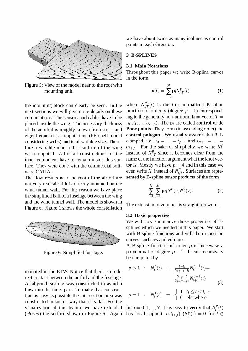
Figure 5:View of the model near to the root withmounting unit.

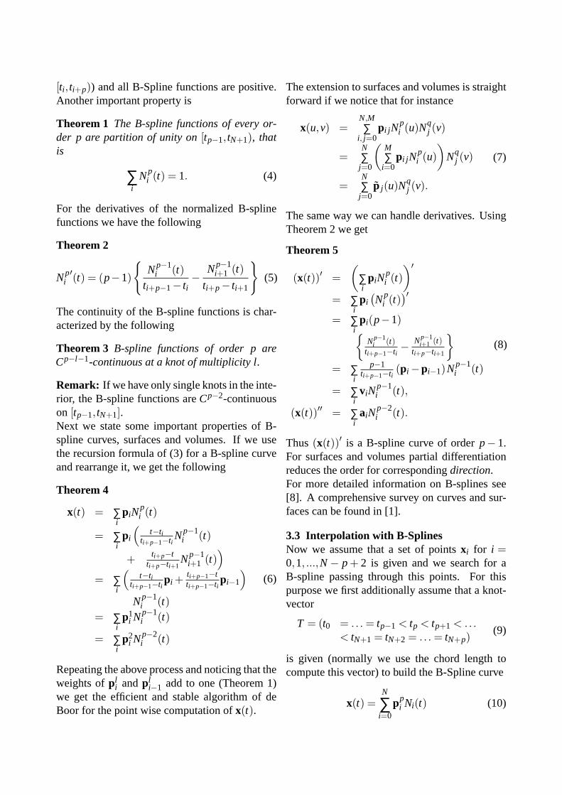
the mounting block can clearly be seen. In thenext sections we will give more details on thesecomputations. The sensors and cables have to beplaced inside the wing. The necessary thicknessof the aerofoil is roughly known from stress andeigenfrequencies computations (FE shell modelconsidering webs) and is of variable size. There-fore a variable inner offset surface of the wingwas computed. All detail constructions for theinner equipment have to remain inside this sur-face. They were done with the commercial soft-ware CATIA.The flow results near the root of the airfoil arenot very realistic if it is directly mounted on thewind tunnel wall. For this reason we have placethe simplified half of a fuselage between the wingand the wind tunnel wall. The model is shown inFigure 6. Figure 1 shows the whole constellation

Figure 6:Simplified fuselage.

mounted in the ETW. Notice that there is no di-rect contact between the airfoil and the fuselage.A labyrinth-sealing was constructed to avoid aflow into the inner part. To make that construc-tion as easy as possible the intersection area wasconstructed in such a way that it is flat. For thevisualization of this feature we have extended(closed) the surface shown in Figure 6. Again

we have about twice as many isolines as controlpoints in each direction.

3 B-SPLINES

3.1 Main NotationsThroughout this paper we write B-spline curvesin the form

x(t) =N

∑i=0

piNpi,T(t) (1)

where Npi,T(t) is the i-th normalized B-spline

function of orderp (degreep− 1) correspond-ing to the generally non-uniform knot vectorT =(t0, t1, . . . , tN+p). Thepi are calledcontrol or deBoor points. They form (in ascending order) thecontrol polygon. We usually assume thatT isclamped, i.e.,t0 = . . . = tp−1 and tN+1 = . . . =tN+p. For the sake of simplicity we writeNp

iinstead ofNp

i,T since it becomes clear from thename of the function argument what the knot vec-tor is. Mostly we havep = 4 and in this case weeven writeNi instead ofNp

i,T . Surfaces are repre-sented by B-spline tensor products of the form

N

∑i=0

M

∑j=0

pi j Npi (u)Nq

j (v). (2)

The extension to volumes is straight foreword.

3.2 Basic propertiesWe will now summarize those properties of B-splines which we needed in this paper. We startwith B-spline functions and will then report oncurves, surfaces and volumes.A B-spline function of orderp is piecewise apolynomial of degreep− 1. It can recursivelybe computed by

p > 1 : Npi (t) = t−ti

ti+p−1−tiNp−1

i (t)+

ti+p−tti+p−ti+1

Np−1i+1 (t)

p = 1 : N1i (t) =

{1 ti ≤ t < ti+1

0 elsewhere

(3)

for i = 0,1, ...,N. It is easy to verify thatNpi (t)

has local support[ti , ti+p) (Npi (t) = 0 for t 6∈

[ti , ti+p)) and all B-Spline functions are positive.Another important property is

Theorem 1 The B-spline functions of every or-der p are partition of unity on[tp−1, tN+1), thatis

∑i

Npi (t) = 1. (4)

For the derivatives of the normalized B-splinefunctions we have the following

Theorem 2

Npi′(t) = (p−1)

{Np−1

i (t)ti+p−1− ti

−Np−1

i+1 (t)ti+p− ti+1

}(5)

The continuity of the B-spline functions is char-acterized by the following

Theorem 3 B-spline functions of order p areCp−l−1-continuous at a knot of multiplicity l.

Remark: If we have only single knots in the inte-rior, the B-spline functions areCp−2-continuouson [tp−1, tN+1].Next we state some important properties of B-spline curves, surfaces and volumes. If we usethe recursion formula of (3) for a B-spline curveand rearrange it, we get the following

Theorem 4

x(t) = ∑i

piNpi (t)

= ∑i

pi

(t−ti

ti+p−1−tiNp−1

i (t)

+ ti+p−tti+p−ti+1

Np−1i+1 (t)

)= ∑

i

(t−ti

ti+p−1−tipi +

ti+p−1−tti+p−1−ti

pi−1

)Np−1

i (t)= ∑

ip1

i Np−1i (t)

= ∑i

p2i Np−2

i (t)

(6)

Repeating the above process and noticing that theweights ofpl

i andpli−1 add to one (Theorem 1)

we get the efficient and stable algorithm of deBoor for the point wise computation ofx(t).

The extension to surfaces and volumes is straightforward if we notice that for instance

x(u,v) =N,M∑

i, j=0pi j N

pi (u)Nq

j (v)

=N∑j=0

(M∑

i=0pi j N

pi (u)

)Nq

j (v)

=N∑j=0

p j(u)Nqj (v).

(7)

The same way we can handle derivatives. UsingTheorem 2 we get

Theorem 5

(x(t))′ =(

∑i

piNpi (t)

)′= ∑

ipi

(Np

i (t))′

= ∑i

pi(p−1){Np−1

i (t)ti+p−1−ti

− Np−1i+1 (t)

ti+p−ti+1

}= ∑

i

p−1ti+p−1−ti

(pi−pi−1)Np−1i (t)

= ∑i

viNp−1i (t),

(x(t))′′ = ∑i

aiNp−2i (t).

(8)

Thus (x(t))′ is a B-spline curve of orderp− 1.For surfaces and volumes partial differentiationreduces the order for correspondingdirection.For more detailed information on B-splines see[8]. A comprehensive survey on curves and sur-faces can be found in [1].

3.3 Interpolation with B-SplinesNow we assume that a set of pointsxi for i =0,1, ...,N− p+ 2 is given and we search for aB-spline passing through this points. For thispurpose we first additionally assume that a knot-vector

T = (t0 = . . . = tp−1 < tp < tp+1 < .. .< tN+1 = tN+2 = . . . = tN+p)

(9)

is given (normally we use the chord length tocompute this vector) to build the B-Spline curve

x(t) =N

∑i=0

ppi Ni(t) (10)

If we want to interpolate at the knots, we get theinterpolating conditions

x(ti+p−1) = xi , i = 0,1, ...,N− p+2. (11)

These areN− p+3 conditions for theN+1 con-trol pointspi . Thus forp = 4 we can formulate2 further conditions. The following four condi-tion sets are of practical use and therefore imple-mented in our system:

a) Vanishing curvature at the beginning and theend of the curve.

b) Given derivatives at the beginning and theend of the curve.

c) Not a knot condition. This means the curveis C3 at the second and last but one interpo-lation point.

d) We construct a periodicC2-continuouscurve (only reasonable ifx0 = xN−2).

Now we place all the control pointspi in a vec-tor of 2D- or 3D-vectorsp and the interpola-tion pointsxi in x. Due to the local support ofthe normalized B-spline functions the conditionx(ti+3) = xi results in a linear equation of theform

αi pi +βi pi+1 + γi pi+2 = xi (12)

with β0 = γ0 = 0 andαN−2 = βN−2 = 0. Vanish-ing curvature yields two equations of the form:

a0p0 +b0p1 +c0p2 = 0aN pN−2 +bN pN−1 +cN pN = 0

(13)

Given derivatives result in:

a0p0 +b0p1 = t0

bN pN−1 +cN pN = tN(14)

If we plug in the equations (13) (or (14) respec-tively) at the second and last but one position weend up with a sparse linear system

Ap = x. (15)

The resulting system matrixA is tridiagonal forthe cases a) and b). The control points can eas-ily be computed from this system inO(N) timeby Gauss-elimination and back substitution after-wards. The not a knot condition results in twoequation with entries for the first five and the lastfive control points. Two pre-elimination steps foreach of them yield a tridiagonal system again.Only for the periodic case d) we have a fill-inin the last column and row during the Gauss-elimination steps. But nevertheless the compu-tation time isO(N) again.For surfaces we get a matrixAu for the u-direction andAv for the v-direction. Now thecollections of control pointsP and interpolationpoints X are matrices of vectors (2D or 3D).Again we have add conditions at the boundarycurves. Notice that at the boundary corners wehave 4 undetermined conditions. This can beresolved by choosing atwist vector(the partialderivativexuv at every corner). In standard litera-ture this is solved the following way: Letvec(S)be the vector obtained by catenating the columnsof a matrix S; first column ofS first, then sec-ond and so on. In MatLab notation this writes asvec(S) = S(:). This concept can be generalized tomatrices of vectors and the 3D case, but there isno direct MatLab notation. By⊗ we denote thestandard tensor product (Kronecker product, see[10] for more details on tensor products). In 2Dthe interpolation conditions result in the follow-ing equivalent equations:

(Av⊗Au)P(:) = X(:). (16)

To avoid tensor product matrices we write the re-sulting interpolation problem in the form

AuPATv = X, (17)

which is equivalent to (16). Now a Gauss-elimination step regardingAu not only works onone column vectorx, but on all columns ofX.Analogous the elimination regardingAv works onall rows ofX. The same is true for back substitu-tion. If we use standard indicesi and j for the ele-ments (3D vectors) ofX we also sayAu acts on all

j andAv on all i. With theL-U-decompositionsAu = LuUu andAv = LvUv this can be written as

AuPATv = LuUuPUT

v LTv = X. (18)

We need the 3D case for the volume grids aroundour models. It is obtained from the tensor prod-uct nature analogous to the 2D case above, butwe cannot use thestandardmatrix notations asin (18). We can only write

(Aw⊗ (Av⊗Au))P(:) = X(:). (19)

Note thatAu, Av andAw are still tridiagonal ma-trices. Now there are the indicesi, j andk for theelements ofX andAu acts on allj,k, Av on all i,kandAw on all i, j of X. Thus our algorithms makeuse of the sparsity of the system matrices in thesame way as above.

3.4 Approximation with B-SplinesIf the data comes from measurements and thusis not exact interpolation leads to non smoothcurves. For this reason we need methods for ap-proximation and fairing. Figure 2 shows an ex-ample obtained with our methods. Since thereare some constraints like fixed points, tangentsand curvature usual CAD Systems can not beused for our approximation task. Thus we haveto develop special algorithms for this stage ofour modeling process. If we have more datapoints and constraints than control points we canno longer fulfill the equations like (15), (18) or(19). Instead we solve the corresponding (lin-ear) least squares problem. If the problem is oftensor product structure we have similar equa-tions as above. But know the systems are ofbandwidth four and over-determined. Thereforewe replace theL-U-decomposition by theQ-R-decomposition. For (15) this is straight foreword

‖Ap− x‖2 = ‖QRp− x‖2

= ‖Rp−QT x‖2.(20)

The upper part (N+1 equations) can be solved byback substitution. In the lower part we have onlyzeros inR and the corresponding right hand sidegives us the residual of the overall problem.

For surfaces and volumes the situation is a lit-tle bit more complicated. We still want to usethe structure of (18) instead of (16) for ourQ-R-decomposition. At a first glance this is a slightmodification of the standard least squares ap-proximation that rapidly brings down computa-tional time and space. In the surface case thiscan still be written in standard matrix notation asfollows: ∥∥AuPAT

v − X∥∥

2 =∥∥QuRuP(QvRv)T − X∥∥

2 =∥∥RuPRTv −QT

u XQv∥∥

2 →min

(21)

P is computed by backward substitution from leftwith Ru and right withRT

v on the upper left part ofQT

u X Qv. Thus we have minimized the 2-norm in-stead of the Frobenius-norm, which correspondsto the standard least squares approximation.The following theorem is known

Theorem 6 Let A∈ IRm×n with m≥ n. Then

‖A‖2≤ ‖A‖F ≤√

n‖A‖2. (22)

But we can proof that for matrices arising fromtensor products like (21) in the above theoremequality holds between the Frobenius- and the 2-norm. Furthermore this result can be extended tothe case of volumes. Thus it leads to algorithmsfor the standard 2-norm approximation. Theircomplexity is nearly proportional to the numberof approximation points.If there is no tensor product structure we switchto an iterative method. We have decided to useCGLS, a Conjugate Gradient method for linearLeast Squares (also called CGNR in [11]). Thecomplexity is governed by two (sparse) matrix-vector multiplications withA and AT . Abovewe have totally avoided the normal equations forleast squares problems, because they are ill con-ditioned (huge condition number ofAT A) veryoften. Using CGLS we still avoid to buildAT Aand having the huge condition number regard-ing precision, but we can not avoid its influenceon the convergence rate. Notice thatA andAT

are sparse matrices, butAT A is not. Using B-splines of orderp = 4 surface points depend on

at most 16 control points and volumes of at most64. These values limit the number of non zero en-tries inA. Therefore CGLS is an efficient methodto solve the least squares problems arising fromB-splines because it makes extensive use of thesparsity of the system matrix.

4 SOME SPECIAL STAGES OF THE THECONSTRUCTION

In this chapter we will give some details on se-lected steps of the construction. The propertiesstated in the previous section will intensively beused.

4.1 The reference cross-sectionIn our case the cross-section was given by mea-surements in form of ordinates for points Thuswe have to start our considerations with a (pla-nar) cloud ofM + 1 sorted pointsx j . For theparameterization we compute the chord length(CAGD meaning) knot spacing of the corre-sponding curvex(t). It gives us an initial guess ofthe parameter valuest j for x j . From the sequencet j we build theN− p+3 interior knotsti in such away that the density of theti accords to that of thet j . The wanted toleranceε (maximum distancebetween given points and final curve) is split intoε = ε1 + ε2, the tolerance for the approximationand that for the fairing process. The number ofcontrol points is adapted in such a way, that ourcurve fulfills

maxj

mint‖x j −x(t)‖2≤ ε1. (23)

This is done for instance by repeatedly solving(20) until we get the smallestN that fulfills (23).Additionally we adjust the parameterization ofthe curve to arc length. It is much easier to ful-fill the constraints on tangents and curvature inthat form. For more details on such approxima-tion problems see [7]. In a second step the fairingis done in such a way that the third derivative isclose to a constant. For this process the move-ments of the control points is restricted by thedistanceε2 to guarantee that the overall error islimited by ε. The results can be found in Fig-ure 2. The last step on the cross-sections is the

split according to Figure 4. After that we canconstruct the blend to the mounting unit. Thecontrol points of the top and bottom surface canbe seen in Figure 7

Figure 7:Control points of blend and mountingunit.

4.2 The simplified fuselageIn Figure 6 we have already seen the shape of asimplified fuselage and the control points of theB-spline surface representing it. We start the con-struction with a 2D sketch of the cross-sections intwo orthogonal directions (see Figure 8). Theyare modeled as B-splines. The next step is tocompute a periodical surface that passes thesecross-sections. We use elliptical arcs for this pur-pose. Then a cylindrical part is place in the mid-dle of the surface. This done by inserting knots,and stretching the parameterization and the con-trol points on a straight line. Finally we take carethat enough control points are planar to guaran-tee that the intersection with the wing is planar(compare section 2).

4.3 Winglet constructionIn [5] algorithms for generating airplane wingsfor numerical simulation and manufacturingwere presented. We have enhanced the methodsgiven there by algorithms for winglet construc-tions. A final result is shown in Figure 9. The ba-sic idea is to determine the necessary parametersin top and front view and then do all computa-tions directly on the control points. The requiredmodifications on the top view (compare Figure 3)are shown in Figure 10. Again WinCAG is usedfor these construction steps. We mark the bend-

fro

nt

curv

e

ba

ck c

urv

e

off

set

for

fron

t a

nd

ba

ck

mid

dle

cu

rve

off

set

mid

dle

cu

rve

20m

m o

rth

og

on

al

Figure 8:Sketches for the fuselage.

ing positionx0 and add an additional dihedral an-glea. From this the new positionsA′4 andA′5 andthe wing chordsl ′4 and l ′5 are determined. Thesuggestion forR′ is to use the same shorteningas in the original case without the winglet. Nextimagine a horizontal wing inx-direction and the(horizontal) plane of the wing chords (z= 0). Inthis plane the control points of our surfaces have(x,y)-coordinates and a certain height (positiveor negative). Bending the plane at an axis iny-direction with radiusr (see Figure 11) we trans-form the (x,y)-coordinates of the control points.Then we add their previous height perpendicularto the bended plane receiving the control pointsof the patches describing the winglet and its tip.

Figure 9:Winglet.

R’

A3

l3

A4’

l4’

x0

a

A5’

l5’

Figure 10:Winglet construction - top view.

To receive satisfactory results several knots haveto be inserted for thex-direction (see Figure 11).

ra/2

x2 x1 x0d

d

c" c

x’2

c’

x’1

C

Figure 11:Winglet construction - front view.

5 CONCLUSIONSIn this paper we have described the use of B-spline techniques for the automated generationof sparse, watertight B-spline models for windtunnel wing-fuselage configurations. Classicaltools have been modified and adapted to the spe-cial requirements of this project. The resulting

geometry can be transferred without conversionsor approximations between the various softwarewhich was used for the manufacturing, techni-cal construction and grid generation by IGESfiles. Moreover, the parameters of the construc-tion, like profile ordinates, bending radii, sweepangle, etc. can easily be modified since the mod-eling algorithms have been automated.

ACKNOWLEDGMENTSThis work has been performed with fundingby the Deutsche Forschungsgemeinschaft in theCollaborative Research Center SFB401 ”FlowModulation and Fluid Structure Interaction atAirplane Wings” of the RWTH Aachen, Univer-sity of Technology, Aachen, Germany.

REFERENCES[1] Bohm, W., Farin, G. and Kahmann, J. A sur-

vey of curves and surface methods in CAGD.Computer Aided Geometric Design 1, 1–60,1984.

[2] Brakhage, K.-H. Ein menugesteuertes, intel-ligentes System zur zwei- und dreidimen-sionalen Computergeometrie, VDI Reihe20 CAD/CAM, Nr. 26 Edition. VDI Ver-lag,1990.

[3] Brakhage, K.-H., Lamby, Ph., Muller, S.et all. H-adaptive multiscale schemes forthe compressible navier-stokes equations —polyhedral discretization, data compressionand mesh generations. In J. Ballmann, ed-itor, Flow Modulation and Fluid-Structure-Interaction at Airplane Wings, volume 84 ofNumerical Notes on Fluid Mechanics, pages125–204. Springer, 2003.

[4] Brakhage, K.-H. Wincag-education softwarefor geometry. In: Proceedings of th 11th In-ternational Conference on Engineering Com-puter Graphics and Descriptive Geometry.Guangzhou, China, August 1-5 2004.

[5] Brakhage, K.-H. and Lamby, Ph. Generatingairplane wings for numerical simulation andmanufacturing. In Soni B.K. et all, editor,9th

International Conference on Numerical GridGeneration in Computational Field Simula-tions, San Jose, USA, June 11-18 2005.

[6] Brakhage, K.-H. and Lamby, Ph. Numeri-cal Grid Generation for Solving the Navier-Stokes Equations using B-Spline Tech-niques. In Soni B.K. et all, editor,9th In-ternational Conference on Numerical GridGeneration in Computational Field Simula-tions, San Jose, USA, June 11-18 2005.

[7] Brakhage, K.-H. and Lamby, Ph. Applicationof B-Spline Techniques to the Modeling ofAirplane Wings and Numerical Grid Genera-tion. Submitted to Computer Aided Geomet-ric Design, (IGPM preprint 2007).

[8] Farin, G., Curves and Surfaces forComputer-Aided Geometric Design.Academic Press, 4th edition (September1996).

[9] Moir, I. Measurements on a two-dimensionalaerofoil with high lift devices. AGARD-AR-303 Vol. I+II, DRA, Farnborough, 1994.

[10] Pitsianis, N.P. The Kronecker Product inApproximation and Fast Transform Genera-tion. Cornell University, 1997, (Dissertation)

[11] Saad, Y. Iterative Methods for Sparse Lin-ear Systems, 2nd Edition. SIAM, 2003.

ABOUT THE AUTHORKarl-Heinz Brakhage is member of the Insti-tute of Geometry and Numerical Mathematicsat the Aachen University of Technology. Hisresearch interests are Computer Aided Geomet-ric Design, CAx Technologies, Grid Genera-tion, Scientific Computing, Computer Graphics,and Development of Education Software. Hecan be reached by e-mail: brakhage@igpm.rwth-aachen.de, by Fax: +49(241)8092317, by phone:+49(241)8096591, the postal address: Inst.of Geometry and Numerical Mathematics /RWTH Aachen / Templergraben 55 / D-52056Aachen, Germany, or through the Web site:www.igpm.rwth-aachen.de/brakhage