Spin glasses in a ﬁeld - Chimera: A WWW Server in Rome

Diluted one-dimensional spin glasses with long-range interactions undergo a phase transition in presence of an external magnetic field

Federico Ricci-Tersenghi!(Università La Sapienza)

Spin glasses in a field

113th Statistical Mechanics Conference!Rutgers University May 10, 2015

in honor of E. Brezin, G. Jona-Lasinio and G. Parisi

Giorgio, me and the computers• 20 years of intense interactions!• Mainly mentoring, thanks Giorgio!!• Computer programming is not writing a code…!

- optimization!- search for new models and tools of analysis!- always with a clear physical picture in mind!

• Uncovering new physics with a computer is an “art”……and Giorgio is an artist ;-)!

• Building most powerful computers: APE100, APEmille, Janus and Janus II!- essential for studying non-perturbative effects

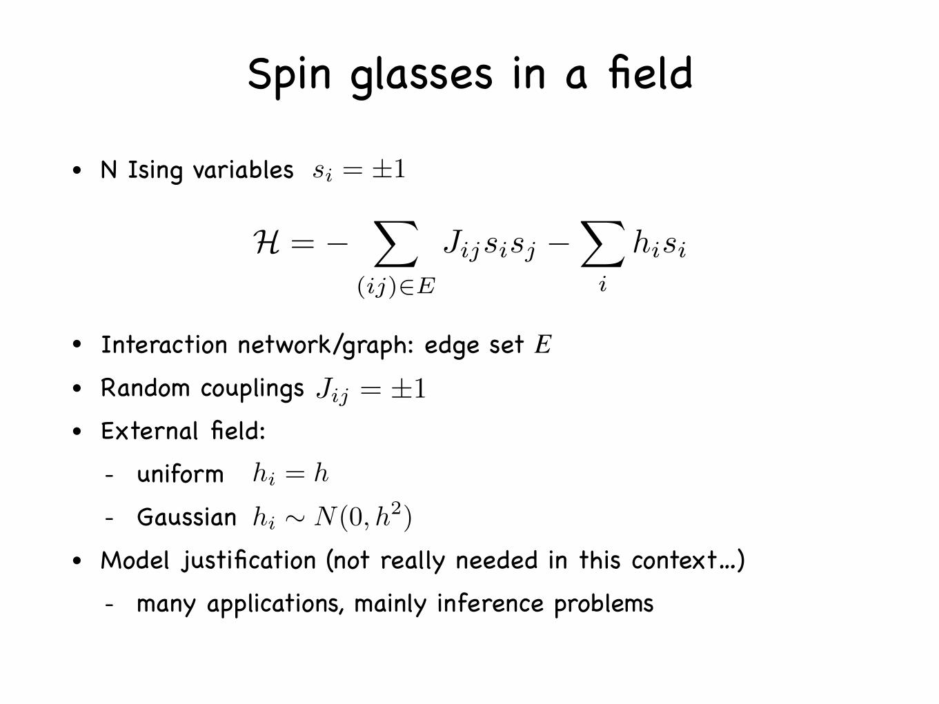
Spin glasses in a field• N Ising variables !

• Interaction network/graph: edge set E!• Random couplings!• External field:!

- uniform!- Gaussian!

• Model justification (not really needed in this context…)!- many applications, mainly inference problems

H = X

(ij)2E

Jijsisj X

i

hisi

si = ±1

Jij = ±1

hi = h

hi N(0, h2)

• E is the complete graph!• rescale J by !• Parisi solution: full replica symmetry breaking (FRSB)!• Overlap between 2 configurations s and t is!• many “states” and broad P(q) below dAT line Tc(h)

Fully connected, SK model

1/pN

P (q) P (q)T > Tc T < Tc

qEA qmin qmax

q N1X

i

siti

Sparse random graphs• Erdos-Renyi (ER), random regular graph (RRG)!• finite degree -> local fluctuations

(more similar to low-dimensional lattices)!• mean-field approx. not valid

-> Bethe-Peierls approx.(Mézard & Parisi, 2001)!

• analytically known:!- RS & 1RSB solutions !- critical properties!- non-diverging dAT line!

• FRSB is a challenging…

We construct the random regular graph in the following way: we attach c legs toeach vertex and then we recursively join a pair of legs, forming a link, until no legsare left or a dead end is reached (this may happen because we avoid self-linking of avertex and double-linking between the same pair of vertices); if a dead end is reached,the whole construction is started from scratch.

Similarly to the Sherrrington–Kirkpatrick model, the model (2) has a continuousspin glass phase transition at a critical temperature Tc which depends both on thevalue of c and H. At variance with the Sherrrington–Kirkpatrick model, the criticalline in the (T,H ) plane does not diverge when T! 0, but rather reaches a finite valueHc (see Figure 1). This is due to the finite number of neighbors each spin has on arandom graph of finite mean degree (while this number is divergent with the systemsize in the Sherrrington–Kirkpatrick model). In this sense the present model is closerto finite dimensional models than the Sherrrington–Kirkpatrick model is.

The replica symmetric (RS) phase of model (2) can be solved analytically by thecavity method [13]. In particular one can find the boundary of the RS phase, beyondwhich the model solution spontaneously breaks the replica symmetry [15,16]. InFigure 1 we show such a critical line in the (T,H ) plane for the model with fixeddegree c¼ 4. The high-temperature and/or high-field region is replica symmetric,while a breaking of the replica symmetry is required in the low-temperature and low-field region. We have checked that the phase boundary behaves likeHc(T )/ (T"Tc)

3/2 close to the zero-field critical point Tc, and the exponent is thesame as that found in the Sherrrington–Kirkpatrick model.

We have carried our Monte Carlo simulations at the point marked with the bigdot in Figure 1, that is H¼ 0.7 and T¼ 0.73536. The uncertainty in the criticaltemperature for H¼ 0.7 is 10"5. At that point the value of the thermodynamicoverlap is q0¼ 0.67658(1). Please note that we have chosen a rather large value of the

0

0.2

0.4

0.6

0.8

1

1.2

1.4

1.6

0 0.2 0.4 0.6 0.8 1 1.2 1.4 1.6

H

T

RS

RSB

Figure 1. (Color online). Phase diagram in the temperature–field plane for the J¼#1 spinglass model defined on a Bethe lattice of fixed degree c¼ 4. In this work we report datacollected at the critical point marked by the big dot.

Philosophical Magazine 343

Dow

nloa

ded

by [B

iblio

teca

Uni

vers

idad

Com

plut

ense

de

Mad

rid] a

t 05:

29 0

6 Se

ptem

ber 2

012

hc(T = 0) < 1

Spin glasses on RRG• Ideal for comparing analytics and numerics!

- Monte Carlo running time O(N)!- estimate of the critical temperature via the crossing of the

scaled susceptibility N 13SG

SG =

Zdr G(r)

G(r) = hs0sri2c

Takahashi, FRT, Kabashima, PRB (2010)

In the last relation, we have used again the scaling relationfor !min, and h!x" is another well-behaved function that isproportional to x for #x#"1 and converges to a certain con-stant as x→#. Combining the two contributions, we obtainthe finite-size scaling relation of $SG as

$SG $ N!1−%"/!1+%"g!tN!1−%"/!1+%"" + t−1h!tN!1−%"/!1+%""

= N!1−%"/!1+%"F!tN!1−%"/!1+%"" , !20"

where F!x"%g!x"+h!x" /x. The properties of g!x" and h!x"guarantee that F!0" is a finite constant and F!x"&1+O!x−1" for x&1.

For H=0 and C'3, %=1 /2 yields the scaling law $SG=N1/3F!tN1/3". This relation was often assumed in earlierstudies on SG models of the mean-field type.9,22,23 However,as far as the authors know, there has been no numerical vali-dation of this relation, in particular, for the scaling exponentwith respect to t= #T−Tc# /Tc, even for the case of H=0. Inaddition, there is no theoretical guarantee that %=1 /2 alwaysholds for H(0 case. As there are only few analyticalschemes available for dealing with SG models of finite di-mension, we need to build up a solid basis for numericalstudies. Circumstantially comparing the results of numericalexperiments and theoretical predictions of Eqs. !6" and !20"for the current system is a great step toward fulfilling thispurpose.

IV. NUMERICAL EXPERIMENTS

In order to verify the above-mentioned behavior aroundthe AT instability, we performed large numerical experimentson systems with C=4 and sizes N=25 ,26 , . . . ,210, using thereplica exchange !parallel tempering" Markov chain MonteCarlo !MC" method.24,25 Apart from some test runs on smallsystems with H=0, we ran extensive simulations on fieldsH=0.1. 0.2, and 0.3 at, respectively, 33, 34, and 36 differenttemperatures distributed around Tc. For equilibrating the sys-tems, we performed 221 MC sweeps !MCSs" and computedthermal averages from 221 more MCSs after the equilibrationtime. Equilibration was tested by comparing the averagesobtained by using half and one quarter of the total MCSs. Toaccelerate equilibration, replicas of adjacent temperatureswere exchanged once every 30 MCSs. We simulated 16 000samples for each size.

Figure 2 shows the results of runs with H=0. The spin-glass susceptibility rescaled by a factor N−1/3 !correspondingto %=1 /2" nicely crosses at the critical temperature, as pre-dicted analytically. The inset should show the scaling func-tion !if finite-size effects were absent" but we can clearly seethat the data collapse is good only in the high temperature!low )=T−1" region.

Next, let us turn to the case of external fields. Expanding!'SiSj(− 'Si('Sj("2 as

'SiSj('SiSj( − 2'SiSj('Si('Sj( + 'Si('Sj('Si('Sj(

and using different real replicas for computing different ther-mal averages at the same time, the above equation becomes

'Si1Sj

1Si2Sj

2( − 2'Si1Sj

1Si2Sj

3( + 'Si1Sj

2Si3Sj

4( ,

we can write the spin-glass susceptibility $SG as

$SG = N!'q122 ( − 2'q12q13( + 'q13q24("

= N!'q122 ( − 2'q12q13( + 'q12(2" , !21"

where qab=N−1)i=1N Si

aSib is the overlap between two replicas.

Actually we computed $SG in Eq. !21" by measuring over-laps from four different replicas a ,b=1,2 ,3 ,4 evolving in-dependently, in order to reduce correlations effects and thenoise-to-signal ratio.

Figure 3 compares the susceptibilities $SG measured nu-merically on systems of sizes N=26 ,28 ,210 with the onescomputed analytically on the Bethe tree for H=0.1, 0.2, and0.3. We see that the numerical data at high temperaturesconverge nicely to the theoretical estimates on the Bethe tree.Note that the diameter of the regular random graph with C=4 is only ln!N" / ln!C−1"$6.3 even for the case of N=210.This indicates that accuracy of the Bethe approximation isnot determined only by the size of the graphs or, more pre-cisely, by the length of the shortest loops. The relativestrength of the self-interactions compared to the size of thegraphs plays a key role in determining the accuracy. In otherwords, even if the graph contains many loops, which maysignificantly contribute to self-interaction terms !that aremissing on trees", the lack of correlation in the topologymakes the net contribution of these loops very small. Thefinal result is that the critical window size for the suscepti-bilities scales as an inverse power of N rather than 1 / ln N.

Figure 3 !top" shows the analytical curves correspondingto H=0 and H=0.1. One can see how the H=0.1 data closelyfollow the H=0 curve as long as T*Tc!H=0". Only belowTc!H=0" does the data change its curvature and acquire thecorrect linear behavior in T−Tc!H=0.1". Unfortunately, thischange happens at very large values of $SG, and thus, theasymptotic scaling behavior may be difficult to observe. Forlarger fields, H=0.2 and H=0.3, the influence of the H=0fixed point is weaker and the theoretical susceptibility curvesare qualitatively similar to the H=0 curve, with the linearpart in T−Tc extending over a wider range. Nonetheless, forthese larger fields, the values of $SG are much smaller, andthus, the asymptotic behavior may be difficult to observe inthis case as well.

0.1

1

10

100

0.5 1 1.5 2 2.5 3 3.5

χ SG

N-1

/3

T

Tc

N=28

N=27

N=26

N=25

0.1

1

10

-2 -1 0 1 2

χ SG

N-1

/3

(β - βc) N1/3

FIG. 2. !Color online" Rescaled spin-glass susceptibility $SGwithout external field.

FINITE-SIZE SCALING OF THE DE ALMEIDA–… PHYSICAL REVIEW B 81, 174407 !2010"

174407-5

c = 4, h = 0

Spin glasses in field on RRG• Strong finite size corrections!

- crossing points of are far from analytical predictions

We tried to identify the critical point, Tc, from the finite-size scaling of the numerical data, by using !=1 /2 for anyfield value. For this, we plotted N−1/3"SG versus temperatureand looked for a crossing point of data sets having differentN, which should correspond to Tc in the thermodynamiclimit. We see from Fig. 4 that finite-size corrections arerather large, especially for H=0.1 and H=0.3, and changesign depending on the value of the field. The insets in Fig. 4zoom in on the region containing the crossings for all data, to

reveal whether or not the crossings move toward the analyti-cal Tc value computed under the tree approximation. TheH=0.1 crossing points move in the right direction but theydo so very slowly; most probably due to the H=0 fixed pointat Tc!H=0"#1.52 in the vicinity. The H=0.3 crossing pointsalso move toward Tc and do so faster than those of H=0.1,although they come from the low-temperature phase. TheH=0.2 crossing points are more complex, because the cross-

0

0.1

0.2

0.3

0.4

0.5

1 1.2 1.4 1.6 1.8 2 2.2 2.4

χ SG

- 1

T

H = 0.1Tc

N = 26

N = 28

N = 210

tree H = 0.1tree H = 0.0

0

0.1

0.2

0.3

0.4

0.5

1 1.2 1.4 1.6 1.8 2 2.2 2.4

χ SG

- 1

T

H = 0.2Tc

N = 26

N = 28

N = 210


0

0.1

0.2

0.3

0.4

0.5

1 1.2 1.4 1.6 1.8 2 2.2 2.4

χ SG

- 1

T

H = 0.3Tc

N = 26

N = 28

N = 210


(b)

(a)

(c)

FIG. 3. !Color online" Inverse of the spin-glass susceptibilityversus temperature for fields H=0.1 !top", H=0.2 !middle", and H=0.3 !bottom".

0.1

1

10

0.8 1 1.2 1.4 1.6 1.8 2 2.2 2.4 2.6

χ SG

N-1

/3

T

H = 0.1

Tc

N = 210

N = 28

N = 26

1.5

2

2.5

3

1.3 1.35 1.4 1.45

Tc

0.1

1

10

0.8 1 1.2 1.4 1.6 1.8 2 2.2 2.4 2.6

χ SG

N-1

/3

T

H = 0.2

Tc

N = 210

N = 28

N = 26

1.5

1.75

2

2.25

1.05 1.1 1.15 1.2

Tc

0.1

1

10

0.8 1 1.2 1.4 1.6 1.8 2 2.2 2.4 2.6

χ SG

N-1

/3

T

H = 0.3

Tc

N = 210

N = 28

N = 26

1

1.25

1.5

1.75

0.8 0.9 1 1.1

Tc

(b)

(a)

(c)

FIG. 4. !Color online" Rescaled spin-glass susceptibility !as-suming !=1 /2" versus temperature for fields H=0.1 !top", H=0.2!middle", and H=0.3 !bottom". Errors are smaller than the symbolsize.

TAKAHASHI, RICCI-TERSENGHI, AND KABASHIMA PHYSICAL REVIEW B 81, 174407 !2010"

174407-6

We tried to identify the critical point, Tc, from the finite-size scaling of the numerical data, by using !=1 /2 for anyfield value. For this, we plotted N−1/3"SG versus temperatureand looked for a crossing point of data sets having differentN, which should correspond to Tc in the thermodynamiclimit. We see from Fig. 4 that finite-size corrections arerather large, especially for H=0.1 and H=0.3, and changesign depending on the value of the field. The insets in Fig. 4zoom in on the region containing the crossings for all data, to

reveal whether or not the crossings move toward the analyti-cal Tc value computed under the tree approximation. TheH=0.1 crossing points move in the right direction but theydo so very slowly; most probably due to the H=0 fixed pointat Tc!H=0"#1.52 in the vicinity. The H=0.3 crossing pointsalso move toward Tc and do so faster than those of H=0.1,although they come from the low-temperature phase. TheH=0.2 crossing points are more complex, because the cross-

0

0.1

0.2

0.3

0.4

0.5

1 1.2 1.4 1.6 1.8 2 2.2 2.4

χ SG

- 1T

H = 0.1Tc

N = 26

N = 28

N = 210


0

0.1

0.2

0.3

0.4

0.5

1 1.2 1.4 1.6 1.8 2 2.2 2.4

χ SG

- 1

T

H = 0.2Tc

N = 26

N = 28

N = 210


0

0.1

0.2

0.3

0.4

0.5

1 1.2 1.4 1.6 1.8 2 2.2 2.4

χ SG

- 1

T

H = 0.3Tc

N = 26

N = 28

N = 210


(b)

(a)

(c)

FIG. 3. !Color online" Inverse of the spin-glass susceptibilityversus temperature for fields H=0.1 !top", H=0.2 !middle", and H=0.3 !bottom".

0.1

1

10

0.8 1 1.2 1.4 1.6 1.8 2 2.2 2.4 2.6

χ SG

N-1

/3

T

H = 0.1

Tc

N = 210

N = 28

N = 26

1.5

2

2.5

3

1.3 1.35 1.4 1.45

Tc

0.1

1

10

0.8 1 1.2 1.4 1.6 1.8 2 2.2 2.4 2.6

χ SG

N-1

/3

T

H = 0.2

Tc

N = 210

N = 28

N = 26

1.5

1.75

2

2.25

1.05 1.1 1.15 1.2

Tc

0.1

1

10

0.8 1 1.2 1.4 1.6 1.8 2 2.2 2.4 2.6

χ SG

N-1

/3

T

H = 0.3

Tc

N = 210

N = 28

N = 26

1

1.25

1.5

1.75

0.8 0.9 1 1.1

Tc

(b)

(a)

(c)

FIG. 4. !Color online" Rescaled spin-glass susceptibility !as-suming !=1 /2" versus temperature for fields H=0.1 !top", H=0.2!middle", and H=0.3 !bottom". Errors are smaller than the symbolsize.

TAKAHASHI, RICCI-TERSENGHI, AND KABASHIMA PHYSICAL REVIEW B 81, 174407 !2010"

174407-6

N 13SG


h=0.1 h=0.3

Spin glasses in field on RRG• Strong finite size corrections are related to local heterogeneities


!SG "1 − !"C − 1#e−#$Gmax

1 − "C − 1#e−# , "13#

since G cannot tend to infinity when the system is finite.Unfortunately, the following considerations indicate thatsuch a correction is not appropriate for describing the behav-ior in the vicinity of Tc. The right-hand side of Eq. "13# givesGmax when the critical condition 1− "C−1#e−#→0 holds.Gmax grows monotonically as N increases. However, thegrowth rate is only O"ln N# since N%C"C−1#Gmax must holdfor satisfying the constraint concerning the number of nodes.This rate is obviously too slow since numerical experimentsshow that the !SG of finite systems grows as O"N1/3# at thecritical condition, at least, for H=0.9

This discrepancy indicates that effects of self-interactions,which are ignored in the Bethe tree approximation, must betaken into account when evaluating the dependence of !SGon the system size N in the vicinity of Tc. Unfortunately,such an evaluation requires a complicated calculation andstill does not lead to an accurate expression in general.Therefore, to avoid these technical difficulties, we shall em-ploy a phenomenological derivation.

Consider the Hessian A=!−1, where ! denotes a suscep-tibility matrix with elements !ij = "&SiSj'− &Si'&Sj'#. As aworking hypothesis, we assume that the eigenvalues of A,$1%$2% . . . %$N, obey a continuous distribution &"$#,which behaves as

&"$# " "$ − $min#', "14#

close to the lower band edge $min for T(Tc and N→).Moreover, we shall assume for the moment that $min is not

heavily modified by finite corrections. For H=0, an analysisof random matrices of fixed weights, in conjunction withThouless-Anderson-Palmer theory,2 implies that the distribu-tion can be expressed as

&"$;*,+# =1

2,

(4"C − 1#*2 − "$ − +#2

C*2 − "$ − +#2/C, "15#

using certain parameters * and +,20 which supports '=1 /2for C-3. However, here, we do not exclude the possibilitythat ' may depend on T and H. Equation "14# provides an-other expression of !SG,

!SG =1N)

k=1

N

$k−2 → *

$min

d$$−2&"$# " $min−"1−'#, "16#

as N→). Assuming that !SG diverges as O"+t+−1# at critical-ity, $min" t1/"1−'# holds as T approaches Tc from above in thelimit of N→).

However, the statistical fluctuations of the eigenvalues arenot negligible around Tc for large but finite N. As a firstapproximation, therefore, let us regard $k "k=1,2 , . . . ,N# asi.i.d. random variables extracted from &"$#. Since $1 is thesmallest value among the N i.i.d. random variables, thetheory of extreme value statistics21 indicates that magnitudeof the fluctuation of $1 can be evaluated by a simple equa-tion,

N*$min

$1

d$&"$# % O"1# , "17#

which yields a scaling relation $1−$min"N−1/"1+'#.Replacing $min by its scaling relation in terms of t1/"1−'#,

Eq. "17# leads to the following expression for the smallesteigenvalue:

$1 = A1t1/"1−'# + N−1/"1+'#.1

= N−1/"1+'#!A1"tN"1−'#/"1+'##1/"1−'# + .1$ , "18#

where A1 is a constant and .1 is a random variable takingvalues O"1#. This derivation also indicates that $k can beexpressed similarly to Eq. "18# as long as k%O"1#. Accord-ingly, all contributions to !SG from $k with k%O"1# can besummed together in a scaling relation like

1N )

k%O"1#$k

−2 % N"1−'#/"1+'#g"tN"1−'#/"1+'## ,

after being averaged with respect to the .k. Here, g"x# is awell-behaved function which returns O"1# constant for x=0and decays polynomially as 1 /x for x/1.

The contribution from all larger eigenvalues, $k with k%O"N#, to !SG can be written in an integral form similar toEq. "16# by substituting the lower band edge $min with $min+O"N−1/"1+'##,

1N )

k%O"N#$k

−2 % *$min+O"N−1/"1+'##

d$$−2&"$#

" !$min + O"N−1/"1+'##$−"1−'#

% t−1h"tN"1−'#/"1+'## . "19#

−1.6 −1.4 −1.2 −1 −0.8 −0.6 −0.4 −0.2 00

0.2

0.4

0.6

0.8

1

1.2

ν

Ω(ν

)+ln

(C−1

)

H=0.2

H=0.3

H=0.1

H=0

FIG. 1. "Color online# Profiles of rate function 0"1# at theAT criticality for several values of external field H in the caseof C=4. Values of the critical temperatures are shown in TableI. In order to evaluate 0"1#, we first computed #"s#=−limG→)"1 /G#ln"&S0SG'− &S0'&SG'#2s by extrapolating numericaldata for G=1,2 , . . . ,20 to G→). Applying a Legendre transforma-tion to this function yields 0"1# as follows: 1=−"! /!s##"s# and0=−s1−#"s#, where 0 has been parametrized by a conjugate vari-able s. For drawing the profiles shown in the figure, we numericallyevaluated "&S0SG'− &S0'&SG'#2s based on 107 samples of Eq. "11#and varied s in the range of −1%s%9. The profiles for H"0 indi-cate that the dominant values of 1 for the AT criticality "dots# areconsiderably larger than the most probable values of 1 "crosses#.The physical implication of this is that the AT instability for H"0 is induced by a small number of atypically large spincorrelations.

TAKAHASHI, RICCI-TERSENGHI, AND KABASHIMA PHYSICAL REVIEW B 81, 174407 "2010#

174407-4

At criticalityhas a broad probability!distribution for h > 0

h=0.1

h=0.2h=0.3

h = 0 =) G(r) = tanh()r

h > 0 =) G(r) exp( r)

h=0

Spin glasses in field on RRG• Strong finite size corrections also in global quantities

Parisi, FRT, PhilMag (2012)

external field, which is roughly half of the largest critical field value Hc(T¼ 0)’ 1.53,in order to avoid crossover effects that could be due to the vicinity of the zero-fieldcritical point.

Monte Carlo simulations have been performed by using the Metropolisalgorithm and the parallel tempering method: we used 20 temperatures equallyspaced between Tmax¼ 2.0 and Tc¼ 0.73536, and we attempted the swap ofconfigurations at nearest temperatures every 30 Monte Carlo sweeps (MCS). Eachsample (of any size) has been thermalized for 224 MCS and then 1024 measurementshave been taken during another 226 MCS: so there are 216 MCS between twosuccessive measurements and we have checked this number to be larger than theautocorrelation time. We study systems of sizes ranging from N¼ 26 to N¼ 214, withthe number of samples ranging from 5120 for N¼ 26 to 1280 for N¼ 214. We aregoing to present only the data for sizes N" 212 for which we have simulated at least2560 samples; indeed the data for N¼ 213 and N¼ 214 are more noisy (due to thelimited number of samples); moreover we fear that some samples may not beperfectly thermalized even after 226 MCS. By restricting to N" 212 we are fullyconfident about the numerical data.

3. Results

We start by showing in Figure 2 the disorder averaged P(q) for different sizes. Theexponential tail on the left side is evident from the plot (which is on a logarithmicscale): this tail goes far into the negative overlap region for small sizes. In thefollowing we are going to show that this exponential tail is not a feature of typicalsamples, but it is completely due to very rare and atypical samples.

The vertical line at q¼ q0 in Figure 2 marks the location of the delta peak in thethermodynamic limit. By looking at the mean and the variance of P(q) we havechecked how finite size effects decay to zero. We see in Figure 3 that while hq2ic

0.0001

0.001

0.01

0.1

1

10

–1 –0.5 0 0.5 1

P(q

)

q

N = 26

N = 28

N = 210

N = 212

Figure 2. (Color online). Disorder averaged overlap probability distributions P(q) show anexponential tail for q< q0.

344 G. Parisi and F. Ricci-Tersenghi

Dow

nloa

ded

by [B

iblio

teca

Uni

vers

idad

Com

plut

ense

de

Mad

rid] a

t 05:

29 0

6 Se

ptem

ber 2

012

qEA

c=4 h=0.7at criticality

Spin glasses in field on RRG

Parisi, FRT, PhilMag (2012)

c=4 h=0.7 at criticality

qEA

shown in the upper right inset this effective field is larger thanH and thus the overlapdistribution is narrower and centered on a value greater than q0, while the atypicalsamples shown in the upper left inset look as if they were below the critical line, i.e.with a field smaller than H.

Since samples with different effective fields will have different critical temper-atures, it is possible that the main source of sample-to-sample fluctuations can bewell described by a random temperature (or field) term in the effective Hamiltonianas in the case of ferromagnets in a random magnetic field [19–21].

It is also worth noticing that the tails of the distributions shown in the insets ofFigure 5 are Gaussian or even steeper, as expected [22,23]. Indeed, the interpolatingcurves superimposed to the bimodal distributions (lower left and upper right insets)have been obtained by assuming q¼ tanh(h) with a Gaussian distributed local field h.The nonlinear transformation is necessary (and sufficient) to take into account thesmall skewness of the distributions.

In Figure 5 we have presented data only for size N¼ 212, but a natural question ishow sample-to-sample fluctuations vary with the system size. We have found that byincreasing the system size the distribution of the moments shrinks towards thethermodynamic limits (hqi¼ q0 and hq2ic¼ 0) with the expected N"1/3 scalingbehavior. However it is not true that all samples become typical in the thermody-namic limit. In other words, the fraction of atypical samples (e.g. those with abimodal distribution) remains roughly constant. In Figure 6 we show the average

0.0001

0.001

0.01

0.1

1

0.5 0.55 0.6 0.65 0.7 0.75 0.8

q

q2 c

0 1 2 3 4 5

0.2 0.4 0.6 0.8 1

0

5

10

15

20

0.2 0.4 0.6 0.8 1

0 2 4 6 8

10

0.2 0.4 0.6 0.8 1

Figure 5. (Color online). Mean and variance of the 2560 samples of size N¼ 212. Insets showthe overlap probability distribution averaged over a small fraction, 1/128, of samples (those inthe corresponding circle). Solid curves in the insets are Gaussian fits to the data (see text fordetails).

Philosophical Magazine 347

Dow

nloa

ded

by [B

iblio

teca

Uni

vers

idad

Com

plut

ense

de

Mad

rid] a

t 05:

29 0

6 Se

ptem

ber 2

012

2560 samples!of size N=4096

SG

D=4 spin glasses in uniform field• !

in the presence of a magnetic field (see Materials and Methodsfor details). Then, ξ is just the characteristic length for the long-distance decay of GðrÞ. In order to arrive at an appropriate de-finition for finite lattice systems, one typically considers the pro-pagator in Fourier space, GðkÞ, and defines the second-momentcorrelation length ξ2 from a truncated Ornstein-Zernike expan-sion -Eqs. 11 and 12.

We have plotted ξ2 in Fig. 1 for all our lattice sizes and h ¼ 0.3.There is a clear change of regime from the high-temperature be-havior, where we can see a finite enveloping curve, to the growthof the correlation length at low temperatures. We intend to showthat this change of regime actually corresponds to a phase transi-tion, using finite-size scaling (26).

In principle, at the transition point there should be scale invar-iance in the system, meaning that

ξ2∕L ¼ f ξðL1∕νtÞ þ…; t ¼ T − TcðhÞTcðhÞ

; [2]

where ν is the thermal critical exponent and the dots representcorrections to leading scaling, expected to be unimportant forlarge lattice sizes. Therefore, the curves of ξ2∕L for large latticesshould intersect at the critical point t ¼ 0. Previous attempts tofind Tc using this approach, however, have generally concludedthat these intersections cannot be found (or, rather, that the ap-parent intersection point goes to T ¼ 0 as L grows) (18, 19). In-deed, if we look at the top box of Fig. 2, we see that either there isno phase transition or ξ2 is completely in a preasymptotic regime.

Some authors, working with D ¼ 1 models with long-range in-teractions, have already offered an explanation for this apparentlack of scale invariance: the propagator behaves anomalously, butonly for the k ¼ 0 mode (25). This irregular behavior resultsin very strong corrections to the leading scaling term of Eq. 2,because the second-moment correlation length depends onGðk ¼ 0Þ. We have checked numerically that this phenomenonis also at play in our D ¼ 4 system, which is probably a generalconsequence of the presence of Goldstone bosons in the system(seeMaterials and Methods for a discussion of this phenomenon).

In order to avoid this issue, in this paper we take a differentapproach, eschewing ξ2∕L in favor of a new dimensionless ratioas the basic quantity for our finite-size scaling study. In particular,we shall consider ratios of higher momenta:

R12 ¼Gðk1ÞGðk2Þ

; [3]

where k1 ¼ ð2π∕L; 0; 0; 0Þ, k2 ¼ ð2π∕L; 2π∕L; 0; 0Þ (and permu-tations) are the smallest nonzero momenta compatible with theperiodic boundary conditions. Notice that, while our use ofR12 asa basic parameter is not standard, this is not in any way a strangequantity. In fact, it is a universal renormalization-group invariant,whose value in the large-L limit for a paramagnetic system shouldbe R12ðT > TcÞ ¼ 1. At the critical point, however, R12ðTcÞ > 1.For instance, using conformal theory relations (27, 28), we havecomputed the critical ratio exactly for the nondisordered D ¼ 2Ising model: RIsing

12 ðTcÞ ¼ 1.694024….To leading order, R12 should have the same scaling behavior as

ξ2∕L, namely,

R12 ¼ f 12ðL1∕νtÞ þ ½scaling corrections&: [4]

However, because this quantity avoids the anomalous k ¼ 0mode, we expect that corrections to scaling be smaller. Indeed,in the bottom box of Fig. 2 we can see that the improvement in thescaling from the ξ2 case is dramatic. Even though corrections toscaling are noticeable, for large sizes the intersections of thecurves seem to converge. Notice as well that the high values ofR12 in the neighborhood of the intersection point are not onlyfar from the paramagnetic limit of R12 ¼ 1, but also above thebound R12 ≤ 2 that would result from a smooth behavior of thepropagator (see the discussion following Eq. 11).

Therefore, it is our working hypothesis that there is a phasetransition, but one that is affected by large corrections to scaling.To substantiate this statement and actually compute the criticalparameters, we must begin by somehow controlling these correc-tions. This analysis is rather technical, but not critical to our

0

2

4

6

1 1.5 2 2.5

2(T,

h =

0.3)

T

L = 5L = 6L = 8L = 10L = 12L = 16

0

0.5

1

0 1 2

h

T

PARAMAGNETICPHASE

SPIN-GLASSPHASE

Fig. 1. Plot of the secondmoment correlation length ξ2 -Eq. 12- against tem-perature in an external field h ¼ 0.3. There is a clear crossover from the con-vergence to a finite envelope at high T to the more rapid growth at low T. Asthis paper shows, this crossover is caused by the onset of a spin-glass transi-tion. The dotted black line is a fit to a critical divergence as ξ∞2 ∝ ½T − T cðhÞ&−ν,where T c and ν are taken from Table 1. The inset is a sketch of the phasediagram (the de Almeida-Thouless line), including a fit to the Fisher-Sompo-linsky scaling h2

c ðTÞ ≃ AjT − T ð0Þc jβ ð0Þþγ ð0Þ (17). The quantities with a superindex

ð0Þ are the values for the h ¼ 0 critical point (33, 34), so the only free para-meter is the amplitude A. In this and all other figures the error bars representone standard deviation.

1.4

1.6

1.8

2.0

2.2

1.2 1.4 1.6 1.8 2.0 2.2

R12

T

L = 5L = 6L = 8L = 10L = 12L = 16

0.2

0.4

0.6

2/L

Fig. 2. Top: plot of ξ2∕L as a function of temperature for all our lattice sizesat h ¼ 0.15. According to leading-order finite-size scaling, the curves for dif-ferent sizes should intersect at the phase transition point, but this behavior isnot seen in the plot. This apparent lack of scale invariance has led someauthors to conclude that there is no phase transition in this system. Bottom:Same plot of the dimensionless ratio R12, Eq. 3, which should have the sameleading-order scaling as ξ2∕L. Unlike the correlation length, however, R12

does exhibit very clear intersections, signalling the presence of a second-or-der phase transition. The dramatic improvement in the scaling, compared tothe top box, is explained by the pernicious effect on ξ2 of the anomalousbehavior in the correlation function for zero momentum.

Baños et al. PNAS ∣ April 24, 2012 ∣ vol. 109 ∣ no. 17 ∣ 6453

PHYS

ICS

Janus collaboration, PNAS (2012)

autocorrelation times is ensured. The final product is a set of thermalized andalmost independent configurations. As an example, each L ¼ 16 sample inh ¼ 0.15 was simulated at least for 5 × 107 heat bath lattice sweeps at eachof the NT ¼ 32 temperatures (we performed a parallel tempering updateevery 10 heat baths). However, the hardest sample required as many as 2.6 ×1010 heat bath sweeps.

The L ¼ 16 lattices were simulated on the Janus computer with an updatespeed (for each of its 256 units) of 86 ps per spin flip with a heat bath scheme.The L ≤ 12 lattices were simulated on Personal Computer (PC) clusters, with aC code that uses multispin coding (40) with 128-bit words (using the stream-ing extensions); the update speed in this case is 350 ps per spin flip using aMetropolis algorithm (on an Intel Core2 processor at 2.40 GHz). With multi-spin coding, the samples whose simulations have to be extended must beextracted from the original 128-sample bundles to construct new bundlesthat are then extended with the same code. Note finally that, becausethe PC spreads the spin flips over 128 samples, the simulation for each sampleis faster on Janus by a factor approximately 500. This difference is significantwhen the equilibration time is large.

The Correlation Functions. The main quantities that we compute are the cor-relation functions. In the presence of a magnetic field, the expectation ofeach spin Sx is nonvanishing. Hence we may consider these two correlationfunctions:

G1ðrÞ ¼1

L4∑

x

ðhSxSxþri − hSxihSxþriÞ2; [9]

G2ðrÞ ¼1

L4∑

x

ðhSxSxþri2 − hSxi2hSxþri2Þ : [10]

In the above, the h⋯i stands for the thermal average in a single sample, whilethe disorder average is indicated by an overline. Note that the Fourier trans-form G1ðk ¼ 0Þ is the spin-glass susceptibility. We simulate four real replicasfSðaÞ

x g (i.e., four systems with the same couplings evolving independently un-der the thermal noise) in order to obtain unbiased estimators of the correla-tion functions. In the main text G stands for either of the G1;2. In the fits wehave combined data from both whenever it was useful to obtain smaller sta-tistical errors.

The correlation functions were computed off-line over stored configura-tions. We note that configurations at different Monte Carlo times can becombined as long as they belong to different replicas (41). This combination

results in small Monte Carlo errors with a modest number of configurations,so the uncertainty on the final result is dominated by the sample-to-samplefluctuations. This step is rather time consuming, so we also use multispin cod-ing to accomplish it.

In order to define the second-moment correlation length (42), we considerthe following Ornstein-Zernike expansion for the propagator in Fourierspace,

1

GðkÞ¼ ξ2

Gð0Þ

!1

ξ2þ k2 þ a4ðk2Þ2 þ…

"; [11]

where k2 ¼ 4∑μ sin2ðkμ∕2Þ. Then, the common second-moment correlationlength ξ2 is obtained by truncating the expansion at the k2 term:

ξ2 ¼1

2 sinðπ∕LÞ

#Gð0ÞGðk1Þ

− 1

$1∕2

: [12]

As we comment in the main text, this definition is not well behaved forour model, due to the anomalous behavior of the k ¼ 0mode. Actually, thereis a simple, yet unexpected explanation for this anomaly. The anomalous be-havior arises whenever soft excitations (Goldstone bosons) are present in thelow-temperature phase, while an external magnetic field splits excitationsinto longitudinal and transversal (43). Familiar examples of Goldstone bosonsare magnons, or the phonons in an acoustical branch. What is most peculiarabout spin glasses is that soft modes are present (44, 45), even if our variablesare discrete.

ACKNOWLEDGMENTS. We thank Davide Rossetti for introducing us to thehandling of the 128-bit registers. We acknowledge partial financial supportfrom Ministerio de Ciencia e Innovación (MICINN), Spain, (contract nos.FIS2009-12648-C03, FIS2010-16587, TEC2010-19207), from Universidad Com-plutense de Madrid (UCM)-Banco de Santander (GR32/10-A/910383), fromJunta de Extremadura, Spain (contract no. GR10158), and from Universidadde Extremadura (contract no. ACCVII-08). B.S. and D.Y. were supported by theFormación de Profesorado Universitario (FPU) program (Ministerio de Educa-ción, Spain); R.A.B. and J.M.-G. were supported by the Formación de PersonalInvestigador (FPI) program (Diputación de Aragón, Spain); finally J.M.G.-N.was supported by the FPI program (Ministerio de Ciencia e Innovación,Spain).

1. Debenedetti PG (1997) Metastable Liquids (Princeton University Press, Princeton).2. Debenedetti PG, Stillinger FH (2001) Supercooled liquids and the glass transition.

Nature 410:259–267.3. Cavagna A (2009) Supercooled liquids for pedestrians. Phys Rep 476:51–124.4. Mydosh JA (1993) Spin Glasses: an Experimental Introduction (Taylor and Francis,

London).5. Hérisson D, Ocio M (2002) Fluctuation-dissipation ratio of a spin glass in the aging

regime. Phys Rev Lett 88:257202.6. Cruz A, et al. (2001) SUE: A special purpose computer for spin glass models. Computer

Physics Communications 133:165–176.7. Ogielski A (1985) Dynamics of three-dimensional Ising spin glasses in thermal equili-

brium. Phys Rev B 32:7384–7398.8. Belletti F, et al. (2008) Simulating spin systems on IANUS, an FPGA-based computer.

Computer Physics Communications 178:208–216.9. Belletti F, et al. (2008) Nonequilibrium spin-glass dynamics from picoseconds to one

tenth of a second. Phys Rev Lett 101:157201.10. Gunnarsson K, et al. (1991) Static scaling in a short-range Ising spin glass. Phys Rev B

43:8199–8203.11. Ballesteros HG, et al. (2000) Critical behavior of the three-dimensional Ising spin glass.

Phys Rev B 62:14237–14245.12. Palassini M, Caracciolo S (1999) Universal finite-size scaling functions in the 3D Ising

spin glass. Phys Rev Lett 82:5128–5131.13. Bray AJ, MooreMA (2011) Disappearance of the de Almeida-Thouless line in six dimen-

sions. Phys Rev B 83:224408.14. Parisi G, Temesvári T (2011) Replica symmetry breaking in and around six dimensions.

Nucl Phys B 858:293–316.15. Bray AJ, Roberts SA (1980) Renormalization-group approach to the spin glass transi-

tion in finite magnetic fields. J Phys C Solid State 13:5405–5412.16. de Almeida JRL, Thouless DJ (1978) Stability of the Sherrington-Kirkpatrick solution of

a spin glass model. J Phys A 11:983–990.17. Fisher DS, Sompolinsky H (1985) Scaling in spin-glasses. Phys Rev Lett 54:1063–1066.18. Young AP, Katzgraber HG (2004) Absence of an Almeida-Thouless line in three-dimen-

sional spin glasses. Phys Rev Lett 93:207203.19. Jörg T, Katzgraber H, Krzakala F (2008) Behavior of Ising spin glasses in a magnetic

field. Phys Rev Lett 100:197202.

20. Jönsson PE, Takayama H, Aruga Jatori H, Ito A (2005) Dynamical breakdown of theIsing spin-glass order under a magnetic field. Phys Rev B 71:180412.

21. Petit D, Fruchter L, Campbell I (1999) Ordering in a spin glass under applied magneticfield. Phys Rev Lett 83:5130–5133.

22. Petit D, Fruchter L, Campbell I (2002) Ordering in Heisenberg spin glasses. Phys Rev Lett88:207206.

23. Tabata Y, et al. (2010) Existence of a phase transition under finite magnetic field in thelong-range RKKY Ising spin glass DyxY1−xRu2Si2. J Phys Soc Japan 79:123704.

24. Moore M, Drossel B (2002) p-spin model in finite dimensions and its relation to struc-tural glasses. Phys Rev Lett 89:217202.

25. Leuzzi L, Parisi G, Ricci-Tersenghi F, Ruiz-Lorenzo JJ (2009) Ising spin-glass transition ina magnetic field outside the limit of validity of mean-field theory. Phys Rev Lett103:267201.

26. Amit DJ, Martin-Mayor V (2005) Field Theory, the Renormalization Group and CriticalPhenomena (World Scientific, Singapore), third edition.

27. Di Francesco P, Saleur H, Zuber JB (1987) Critical Ising correlation functions in the planeand on the torus. Nucl Phys B 290:527–581.

28. Di Francesco P, Saleur H, Zuber JB (1988) Correlation functions of the critical Ising mod-el on a torus. Europhys Lett 5:95–100.

29. Ballesteros HG, Fernandez LA, Martin-Mayor V, Muñoz Sudupe A (1996) New univers-ality class in three dimensions?: the antiferromagnetic RP2 model. Phys Lett B378:207–212.

30. Billoire A, et al. (2011) Finite-size scaling analysis of the distributions of pseudo-criticaltemperatures in spin glasses. J Stat Mech P10019.

31. Baños RA, et al. (2010) Static versus dynamic heterogeneities in the D ¼ 3

Edwards-Anderson-Ising spin glass. Phys Rev Lett 105:177202.32. Yllanes D (2011) Rugged free-energy landscapes in disordered spin systems (UCM,

Madrid).33. Jörg T, Katzgraber HG (2008) Universality and universal finite-size scaling functions in

four-dimensional Ising spin glasses. Phys Rev B 77:214426.34. Marinari E, Zuliani F (1999) Numerical simulations of the 4D Edwards-Anderson spin

glass with binary couplings. J Phys A 32:7447–7462.35. Fisher DS, Huse DA (1988) Equilibrium behavior of the spin-glass ordered phase. Phys

Rev B 38:386–411.


PHYS

ICS





; [2]





; [3]



ξ2∕L, namely,




0

2

4

6

1 1.5 2 2.5

2(T,

h =

0.3)

T

L = 5L = 6L = 8L = 10L = 12L = 16

0

0.5

1

0 1 2

h

T

PARAMAGNETICPHASE

SPIN-GLASSPHASE




1.4

1.6

1.8

2.0

2.2

1.2 1.4 1.6 1.8 2.0 2.2

R12

T

L = 5L = 6L = 8L = 10L = 12L = 16

0.2

0.4

0.6

2/L




PHYS

ICS





; [2]





; [3]



ξ2∕L, namely,




0

2

4

6

1 1.5 2 2.5

2(T,

h =

0.3)

T

L = 5L = 6L = 8L = 10L = 12L = 16

0

0.5

1

0 1 2

h

T

PARAMAGNETICPHASE

SPIN-GLASSPHASE




1.4

1.6

1.8

2.0

2.2

1.2 1.4 1.6 1.8 2.0 2.2

R12

T

L = 5L = 6L = 8L = 10L = 12L = 16

0.2

0.4

0.6

2/L




PHYS

ICS

h = 0.15

Tc(h = 0) = 2.002(10)

D=3 spin glasses in uniform field• Data from Janus supercomputer:!

- best data currently available!- approaching the experimental timescales…!- …and still strong finite size corrections!!

• Standard methods of analysis -> no phase transition in field

0.1

0.3

0.5

0.7

0.9

ξ L/L

h=0.1

L=32L=24L=16L=12L= 8L= 6L=∞, h=0

1.2

1.5

1.8

2.1

R12

h=0.1

0.1

0.2

0.3

0.4

0.5

0.6

0.5 0.9 1.3 1.7

ξ L/L

T

h=0.2

0.5 0.9 1.3 1.7 1

1.3

1.6

1.9

2.2

R12

T

h=0.2Janus collaboration, JSTAT (2014)

D=3 spin glasses in uniform field• The largest size L=32 at the lowest temperature T=0.805128

still shows strong fluctuations (as in RRG)!

• P(q) should be a delta function in the paramagnetic phase!

Janus collaboration, JSTAT (2014)

J.Stat.M

ech.(2014)P05014

The three-dimensional Ising spin glass in an external magnetic field

Figure 2. The probability distribution function P (q) of the overlap q for ourlargest lattices (L = 32) at the lowest simulated temperature (T = 0.805 128) forall our magnetic fields (h = 0.05, 0.1, 0.2, 0.4), see table 1. The order parameterin the Edwards–Anderson model is the overlap q, and it is defined in the [1, 1]interval (see section 4). The supports are wide, with exponential tails similar tothose in the mean-field model at the dAT transition line [47].

Instead, we can see from figure 2 that its distribution P (q) has a very wide support,with tails that, for small enough magnetic fields, even reach negative values of q. This isprecisely what was observed in the mean-field version of the model on the de Almeida–Thouless line, and it was attributed to the contribution of a few samples [47].

From these arguments it becomes reasonable to think that we may not be simulatinglarge enough lattices to observe the asymptotic nature of the system and that there maybe some hidden behaviour that we are not appreciating.

2.4. Giant fluctuations

In fact, we find that the average values we measure are representative of only a small partof the data set. That is, the average of relevant observables (e.g., the spatial correlationfunction) only represents the small number of measurements that are dominating it. Therest of the measurements are not appreciated by using the average.

Clearly, standard finite-size scaling methods are not adequate for these systems, andwe need to find a way to take all the measurements into account. Recalling the widedistributions of figure 2, it seems reasonable to sort our measurements according to someconditioning variable q related to the overlaps between our replicas (see section 6). In thisway, we find that the average values we measure are given by only a small part of themeasurements. For example, in figure 3 we show the correlation function C(r). We plotfour estimators of C(r): the average (which is the standard quantity studied in almost all,if not all, previous work), the C(r) that corresponds to the median of the q distribution,

doi:10.1088/1742-5468/2014/05/P05014 7

D=3 spin glasses in uniform field• Conditioning on the value of the overlap we get surprises!


G(r)

J.Stat.M

ech.(2014)P05014


Figure 3. Di↵erent instances of the normalized correlation function C(r) (9) forL = 32, T = 0.805 128. The field is h = 0.1 on the left, and h = 0.2 in theright plot. We sort the measurements with the help of a conditioning variate q asdescribed in section 6. In this case q is the median overlap q

med

. We show small setsof measurements, namely the ones with the 10% lowest (top curve) and highest(bottom curve) q and those whose q corresponds to the median of the distributionof q (50% lowest/highest q). This sorting reveals extreme di↵erences in the faunaof measurements. The average and median of the correlation functions are verydi↵erent. The average is very similar to the 10% lowest ranked measures, i.e.,it is only representative of a very small part of the data. We normalize C(r)by dividing by C(0) because we measure point-to-plane correlation functions (9).The correlation functions have zero slope at r = L/2 due to the periodic boundaryconditions.

and the measurements with the 10% highest (lowest) values of q. We see that the averageis very close to the 10% lowest q, and very far from the two other curves. Therefore, whenwe plot the average curve, we are only representing the behaviour of that small set ofdata.

Therefore, if we want to understand the behaviour of the whole collection ofmeasurements, we have to be able to find some criterion to sort them and analyse themseparately.

3. Model and simulations

3.1. The model

We consider a 3D cubic lattice of size L with periodic boundary conditions. In each of theV = L3 vertices of the lattice there is a spin

x

= ±1. The spins interact uniquely withtheir nearest neighbours and with an external magnetic field h. The Hamiltonian is

H = X

hx,yiJxy

x

y

hX

x

x

, (1)

doi:10.1088/1742-5468/2014/05/P05014 8

D=3 spin glasses in uniform field• All measurements from different samples together!• Conditional expectation


E[O|q] = E[O q,q]

E[q,q]E[O] =

ZdP (q)E[O|q]

(Oi, qi)

conditioningvariate

V[O] =

ZdP (q)V[O|q] +

ZdP (q)

E[O|q] E[O]

2

D=3 spin glasses in uniform field• All measurements from different samples together!• Conditional expectation


E[O|q] = E[O q,q]

E[q,q]E[O] =

ZdP (q)E[O|q]

(Oi, qi)

conditioningvariate

V[O] =

ZdP (q)V[O|q] +

ZdP (q)

E[O|q] E[O]

2

as small as possible!(and hopefully!self-averaging)

as large as possible

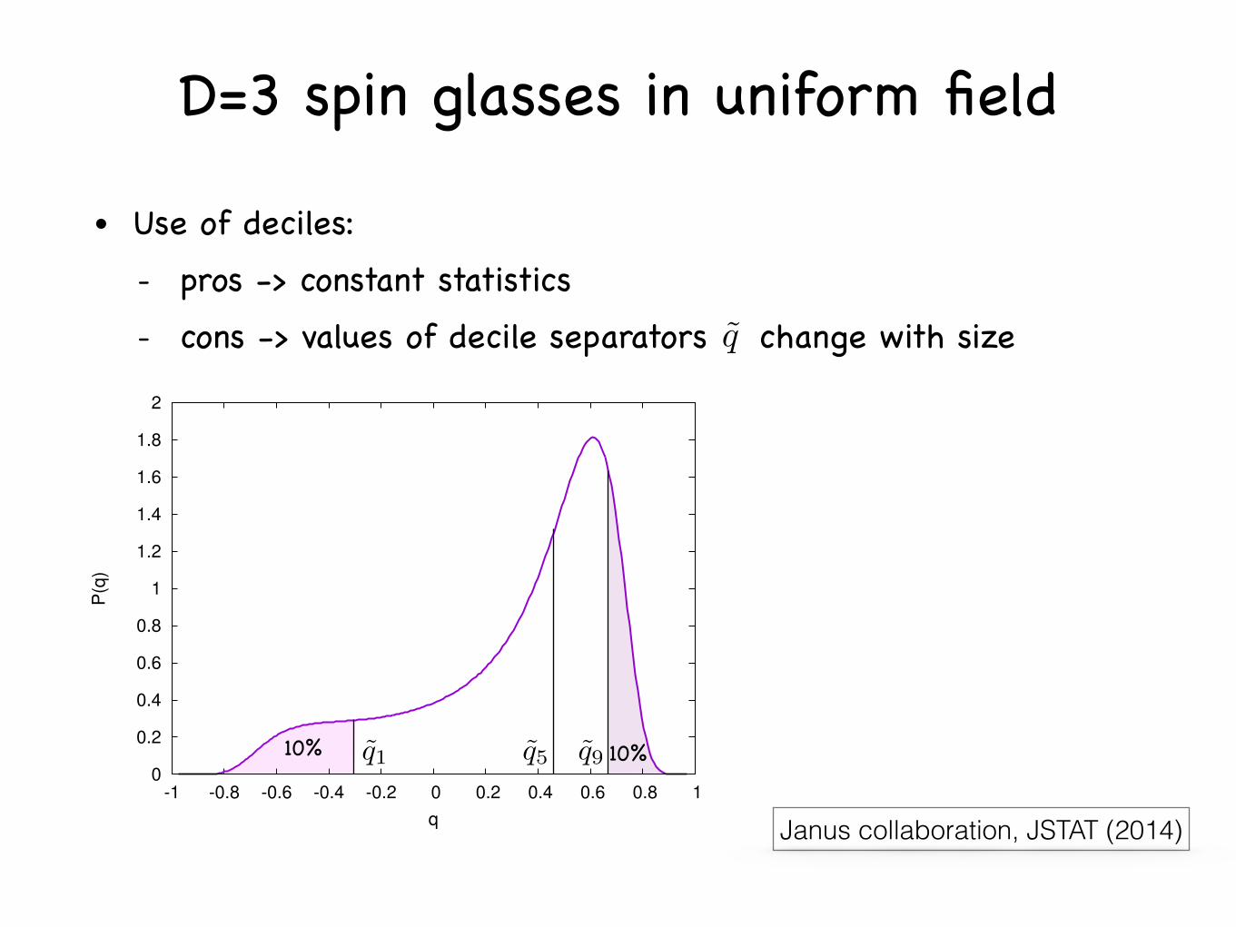
D=3 spin glasses in uniform field• Use of deciles:!

- pros -> constant statistics!- cons -> values of decile separators change with size

0

0.2

0.4

0.6

0.8

1

1.2

1.4

1.6

1.8

2

-1 -0.8 -0.6 -0.4 -0.2 0 0.2 0.4 0.6 0.8 1

P(q

)

q

10% 10%

q

q1 q5 q9


J.Stat.M

ech.(2014)P05014


Figure 8. Finite-size indicators of a phase transition, computed for h = 0.2.On the left side we plot, for quantiles 1 (top), 5 (middle) and 9 (bottom), thecorrelation length in units of the lattice size

L

/L (left) versus the temperature,for all our lattice sizes except L = 6 (we show in appendix D that the quantiledescription is not suitable for L = 6 because there is a double peak in the P (q)).On the right we show analogous plots for R

12

. The vertical line on the left marksthe upper bound T up for a possible phase transition given in [34], while theone on the right marks the zero-field transition temperature T

c

given in [51].Quantile 1 has the same qualitative behaviour of the average

L

/L, shown infigure 1, while quantiles 5 and 9 suggest a scale invariance at some temperatureTh

< T up.

whose qmed

is even lower than q1

. Moreover, one can notice that in figure 1 the indicatorsL

/L and R12

show a di↵erent qualitative behaviour when the lattices are small (R12

showsa crossing). This discrepancy vanishes when we look only at the first quantile: separationof the di↵erent behaviours enhances the consistency between

L

/L and R12

.The behaviour of the fifth quantile is quite di↵erent, since now it appears reasonable

that the curves cross at some T . T up(h). The crossings become even more evident whenwe consider the highest quantile.

doi:10.1088/1742-5468/2014/05/P05014 20

D=3 spin glasses in uniform field

• For T>Tchowever numerical datasensibly depends on the decile!


limL!1

qi = qEA

first decile

median

last decile

J.Stat.M

ech.(2014)P05014


Figure 8. Finite-size indicators of a phase transition, computed for h = 0.2.On the left side we plot, for quantiles 1 (top), 5 (middle) and 9 (bottom), thecorrelation length in units of the lattice size

L

/L (left) versus the temperature,for all our lattice sizes except L = 6 (we show in appendix D that the quantiledescription is not suitable for L = 6 because there is a double peak in the P (q)).On the right we show analogous plots for R

12

. The vertical line on the left marksthe upper bound T up for a possible phase transition given in [34], while theone on the right marks the zero-field transition temperature T

c

given in [51].Quantile 1 has the same qualitative behaviour of the average

L

/L, shown infigure 1, while quantiles 5 and 9 suggest a scale invariance at some temperatureTh

< T up.

whose qmed

is even lower than q1

. Moreover, one can notice that in figure 1 the indicatorsL

/L and R12

show a di↵erent qualitative behaviour when the lattices are small (R12

showsa crossing). This discrepancy vanishes when we look only at the first quantile: separationof the di↵erent behaviours enhances the consistency between

L

/L and R12

.The behaviour of the fifth quantile is quite di↵erent, since now it appears reasonable

that the curves cross at some T . T up(h). The crossings become even more evident whenwe consider the highest quantile.

doi:10.1088/1742-5468/2014/05/P05014 20

D=3 spin glasses in uniform field

• For T>Tchowever numerical datasensibly depends on the decile!


limL!1

qi = qEA

first decile

median

last decile

this minority!dominates theaverage andhides the

phase transition!

Long range interacting D=1 spin glasses • Original proposal (Kotliar, 1983):!

- computationally expensive, running times O(N2)!• Our proposal (Leuzzi, Parisi, FRT, Ruiz-Lorenzo, PRL, 2008)!

- and!- computationally efficient, running times O(N)!- mean-field limit ( ) recovers SG on random graphs

Jij N(0, |i j|)

P[Jij 6= 0] / |i j|Jij = ±1

! 0

no phase transitionmean-field long range

De↵ DU = 61 DL

0 4/3 2

Long range interacting D=1 spin glasses • Original proposal (Kotliar, 1983):!

- computationally expensive, running times O(N2)!• Our proposal (Leuzzi, Parisi, FRT, Ruiz-Lorenzo, PRL, 2008)!

- and!- computationally efficient, running times O(N)!- mean-field limit ( ) recovers SG on random graphs

Jij N(0, |i j|)

P[Jij 6= 0] / |i j|Jij = ±1

! 0

no phase transitionmean-field long range

De↵ DU = 61 DL

0 4/3 2

= 1 + 2/D

Long range interacting D=1 spin glasses • Many pros:!

- very large lattice sizes, up to L = O(104)!- we can increase the effective dimension at no cost

(we are interested in an eventual phase transition for D<6)!- and does not renormalize outside mean-field!- two scaling-invariant

observablesthat cross at the critical point

= 3

/L2

/L

transition vanishes [6], though power-law correlationsmight still be present [14]; this value of the exponent playsthe role of the lower critical dimension in SR systems. Anapproximate relationship between ! and the dimension Dof SR models can be identified as follows. In LR models,the free theory in the replica space is

H ¼ L

4

Z dk

2"ðk!#1 þm2

0ÞX

a!b

j ~QabðkÞj2; (3)

where a and b are replica indices and ~QabðkÞ is the Fouriertransform of the distance-dependent overlap matrix ele-mentQabðrijÞ. Details can be found in Ref. [7]. Comparingthe critical scaling (m0 / jT # Tcj ¼ 0) of Eq. (3) withthat of the free theory for SR spin-glass models in Ddimensions (H & R

dDkk2TrQ2), the following equationturns out to hold close to the upper critical dimension ! ¼1þ 2=D.

We simulate two replicas #ð1;2Þi using the parallel tem-

pering algorithm [16,17]. To study the equilibrium prop-erties, we measure site and link overlaps,

q¼ 1

L

XL

i¼1

#ð1Þi #ð2Þ

i ; ql¼1

zL

X1;L

i;j

J2ij#ð1Þi #ð1Þ

j #ð2Þi #ð2Þ

j ; (4)

and $L ¼ ½%sg=~%ð2"=LÞ # 1(1=ð!#1Þ=½2 sinð"=LÞ(, the

correlation length [18]. %sg ¼ Lhq2i is the spin-glass sus-ceptibility (h) ) )i denotes the thermal average and ) ) )denotes the average over the disorder), and ~%ðkÞ is theFourier transform of the four-point correlation function(~%ð0Þ ¼ %sg). To compute critical properties and finitesize scaling (FSS) corrections, we have used the quotientmethod [19]. We have computed the exponent & from thescaling of the temperature derivative of $L=L and ' fromthe scaling of %sg. As a typical case, we show in Fig. 1 thetemperature and size dependence of %sg and $L. In thequotient method, the estimates of the critical exponent stilldepend on the lattice size: the extrapolation to infinitevolume provides both their asymptotic values and the !exponent of the leading FSS correction, OðL#!Þ. Theresults are summarized in Table II. The ' exponent co-incides with the theoretical prediction ' ¼ 3# ! (' is notrenormalized in the IRD regime [4,7]). Because of strongfinite size effects, this check failed in previous works [8].The & exponent is consistent with the theoretical predic-tion, & ¼ 1=ð!# 1Þ, in the MF case. In the IRD regime,thermodynamic fluctuations dominate and a renormaliza-

tion is necessary: at present only one-loop calculations areavailable [4,7], but their estimates of & are too rough tocompare with numerical data.In the spin-glass phase (T < Tc), site and link overlap

distributions, PðqÞ and PlðqlÞ, can be used as hallmarks todiscriminate among different theories for finite-dimensional spin glasses. Indeed, three cases are contem-plated in the literature. 1. Droplet theory: one state; bothdistributions are delta-shaped. 2. TNT scenario: manystates (q fluctuates), but dropletlike excitations (ql fluctua-tions vanish for large sizes); PðqÞ is broad and PlðqlÞ isdelta-shaped. 3. RSB theory: many states with space-fillingexcitations; both distributions are broad.Distributions PðqÞ and PlðqlÞ for T ’ 0:4Tc are plotted

in Figs. 2 and 3 in a case where MF is exact (! ¼ 5=4) andin an IRD case (! ¼ 3=2), respectively. In both cases, wesee two peaks in the PlðqlÞ for large sizes. Out of MF, sucha result would have been impossible to observe in thismodel with sizes smaller than L ¼ 212.Both distributions seem to be broad, but their thermody-

namic limits must be taken carefully. While it is easy toprove that PðqÞ is not bimodal as L! 1 [lower insets inFigs. 2 and 3 show that Pð0Þ becomes size independent],the limit of PlðqlÞ is more difficult to extract from finitesize data, since its variance converges to a small value, seeupper insets of Figs. 2 and 3 [20]. We provide, thus, analternative method of analysis, testing the hypothesis thatboth q and ql are equivalent measures of the distance

among states [21]. The simplest relation is ql ¼ qaux *Aþ Bq2 þ C

ffiffiffiffiffiffiffiffiffiffiffiffiffiffi1# q2

pz, where z is a normal random vari-

0.1

1

1.55 1.6 1.65 1.7 1.75 1.8 1.85 1.9 1.95

T

κ=8,

10,1

2,14

ρ=3/2χ(

L) L

η-2

10

1

0.1

1.6 1.7 1.8 1.9T

ξ/L

κ=8,

10,1

2,14

FIG. 1. ! ¼ 3=2, IRD regime. Plot of L'#2%sg vs T. Inset:$L=L vs T. Sizes are L ¼ 2(, with ( ¼ 8, 10, 12, 14.

TABLE II. Estimates of critical temperature and exponents.

! ‘‘D’’ Tc 1=& ' ' (th.) !

MF 5=4 8 2.191(5) 0.28(2) 1.751(8) 1.75 0.40(2)IRD 3=2 4 1.758(4) 0.25(3) 1.502(8) 1.5 0.60(6)IRD 5=3 3 1.36(1) 0.19(3) 1.32(1) 1:3!3 0.8(1)

TABLE I. From infinite range to short-range behavior of theSG model defined in Eqs. (1) and (2).

!< 1 Bethe lattice like

1< ! + 4=3 2nd order transition, mean-field (MF)4=3< !< 2 2nd order transition, infrared divergence (IRD)

! ¼ 2 Kosterlitz-Thouless or T ¼ 0 phase transition!> 2 no phase transition

PRL 101, 107203 (2008) P HY S I CA L R EV I EW LE T T E R Sweek ending

5 SEPTEMBER 2008

107203-2

Leuzzi et al. PRL (2008)

Long range D=1 spin glasses with field• Standard tools of analysis:!

- clear phase transition in the mean-field region!- phase transition outside the mean-field region for small fields!- no phase transition for larger fields (e.g. )

affected. FSE are more evident in the large x tail of CðxÞand, thus, at small k in ~CðkÞ, while they decrease as kincreases. The large x part of CðxÞ strongly depends on theaverage overlap order parameter hqi, which is known tohave strong sample-to-sample fluctuations in a field andFSE due to negative overlaps which should disappear in thethermodynamic limit.

With the aim of reducing FSE, we introduce a method

for estimating Tc using ~CðkÞ data with k > 0. We fit ~CðkÞ#1

by a quadratic function Aþ Byþ Cy2 with y ¼½sinðk=2Þ=!'"#1: the resulting fits have a #2=d:o:f: <0:55 (comparable fit qualities have been found in the entireanalysis). As long as T > Tc, we expect limL!1AðL; TÞ ¼##1sg > 0: the inset in Fig. 1 shows the size dependence of~Cð0Þ#1 and AðL; TÞ, with compatible L ! 1 limits.In Fig. 2 we show the best fitting parameter AðL; TÞ for

" ¼ 1:5 and h ¼ 0:1. For each size we compute the tem-perature TcðLÞ by solving the equation AðL; TcðLÞÞ ¼ 0 (inthis way only A > 0 data are used, which are the mostreliable). Finally, we estimate Tc ¼ limL!1TcðLÞ (inset ofFig. 2) and obtain Tc ¼ 1:46ð3Þ. The TcðLÞ scaling in

L#1=$ has an exponent #0:28, in good agreement with1=$ ¼ 0:25ð3Þ for the h ¼ 0 case [15]. On the same data(" ¼ 1:5, h ¼ 0:1) the analysis of the crossing points of#sg=L

2#% and &=L, cf. Eq. (7), is shown in Fig. 3 (rightpanel), yielding no evidence for a phase transition, as inRef. [24]. A very natural explanation is the presence ofstrong corrections to Eq. (7). The case " ¼ 1:4, h ¼ 0:1,provides a still more useful comparison. Our method re-turns a critical temperature Tc ¼ 1:67ð7Þ. Figure 3 shows#sg=L

2#% and &=L vs T: crossings are present, but the

curves seem to merge for T & 1:5 and a precise determi-nation of Tc is practically unfeasible. For " ¼ 1:2, h ¼0:2, the estimate based on the scaling of #sg=L

1=3, Eq. (6),

yields Tc ¼ 1:67ð3Þ, while &=L$=3 curves do not show anycrossing for T > 1:2. Since the transition is MF-like in this

case, the behavior of & is clearly caused by large FSE.Numerical estimates of Tc obtained with the two methodsare reported in Table I and look compatible. It is clear thatfor large " our method works better. As " is decreased, thisnew estimate becomes poorer, because the scaling expo-nent "# 1 [cf. Eq. (8)] is too small to yield a robustextrapolation of AðL; TÞ.Discussion of experimental results.—A possible objec-

tion to the presence of the SG transition (supported by ourresults) is that in experiments on Ising-like SG no dAT linewas detected. Here we consider, in particular, the mostrecent experiments on Fe0:55Mn0:45TiO3 [4], where the acsusceptibilities were accurately measured in the presenceof an external magnetic field. In order to relate externalfields in our model to those used in experiments we look athow much the zero-field-cooled (ZFC) susceptibility atTcðh ¼ 0Þ, #(, decreases as h is increased. In Fig. 4 weplot TcðhÞ=Tcð0Þ vs #(ðhÞ=#(ð0Þ in our model for " ¼ 1:5.In experiments on Fe0:55Mn0:45TiO3 [4] with fields of

4

1

0.4

χ/L1/3

ρ=1.2 (MF) h=0.2

26,....,12

10

0.1

0.001

1.2 1.4 1.6 1.8 2 2.2 T

ξ/Lν/3

ν=5

4

1

0.4

χsg Lη-2

ρ=1.4 2-η=0.4 h=0.1

26,....,12

10

1

0.1

0.01

1.2 1.4 1.6 1.8 2 2.2

ξ/L

T

1

0.4

0.1 ρ=1.5 2-η=0.5 h=0.1

χsg Lη-2

26,....,12

1

0.1

0.01

1.2 1.4 1.6 1.8 2

ξ/L

T

FIG. 3 (color online). Scaling functions vs T. Left panels: " ¼ 1:2, #sg=L1=3 (top) and &=L5=3 (bottom) at h ¼ 0:2. Sizes are L ¼

26; . . . ; 212. Mid panels: " ¼ 1:4, #sg=L0:4 and &=L at h ¼ 0:1. Lower panels: " ¼ 1:5, #sg=L

0:5 and &=L at h ¼ 0:1.

TABLE I. Estimates of Tc: column 4 from Eqs. (6) and (7) andcolumn 5 from the extrapolation of AðL; TÞ by Eq. (8).

" h Tc from #sg Tc from AðL; TÞ1.2 0.0 2.24(1) 2.34(3)1.2 0.1 2.02(2) 1.9(2)

MF 1.2 0.2 1.67(3) 1.4(2)1.2 0.3 1.46(3) 1.5(4)1.25 0.0 2.191(5) 2.23(2)1.4 0.0 1.954(3) 1.970(2)1.4 0.1 )1:5 1.67(7)

IRD 1.4 0.2 )1:1 1.2(2)1.5 0.0 1.758(4) 1.770(5)1.5 0.1 — 1.46(3)1.5 0.15 — 1.20(7)1.5 0.2 — 0.8(2)

PRL 103, 267201 (2009) P HY S I CA L R EV I EW LE T T E R Sweek ending

31 DECEMBER 2009

267201-3

Leuzzi, Parisi, FRT, Ruiz-Lorenzo, PRL (2009)

= 1.4, h = 0.2

Long range D=1 spin glasses with field• A new tool of analysis conditioning on the overlap!

• Claim/conjecture: and are self-averaging!

• At criticality:

bG(k|q) = FT [G(r|q)] bG(k = 0|q) = q2

(q) = bG(k =2

L|q) SG =

ZdP (q)(q)

G(r|q) = hq0qr|qi = E[s0t0srtr|s · t = N q]

P (q) = (q qEA) =) SG = (qEA) / L2

fluctuates much less than(q) SG

G(r|q) (q)

Long range D=1 spin glasses with field• SG phase transition lowering the conditioning overlap!!• Even in the paramagnetic phase!

(q)

L2

0

0.2

0.4

0.6

0.8

1

1.2

-0.8 -0.6 -0.4 -0.2 0 0.2 0.4 0.6 0.8 1

ρ = 1.4 h = 0.2 T = 1.7

q

L = 13L = 12L = 11L = 10

L = 9L = 8

(q)

L2

0

0.5

1

1.5

2

2.5

3

-1 -0.8 -0.6 -0.4 -0.2 0 0.2 0.4 0.6 0.8 1

ρ = 1.4 h = 0.2 T = 1.2

χ(q

) / L

2-η

q

L = 13L = 12L = 11L = 10L = 9L = 8

Long range D=1 spin glasses with field• SG phase transition lowering the conditioning overlap!!• Even in the paramagnetic phase!

(q)

L2

0

0.2

0.4

0.6

0.8

1

1.2

-0.8 -0.6 -0.4 -0.2 0 0.2 0.4 0.6 0.8 1

ρ = 1.4 h = 0.2 T = 1.7

q

L = 13L = 12L = 11L = 10

L = 9L = 8

(q)

L2

0

0.5

1

1.5

2

2.5

3

-1 -0.8 -0.6 -0.4 -0.2 0 0.2 0.4 0.6 0.8 1

ρ = 1.4 h = 0.2 T = 1.2

χ(q

) / L

2-η

q

L = 13L = 12L = 11L = 10L = 9L = 8

qc(T ) qc(T )

Long range D=1 spin glasses with field• Very robust estimate of the critical temperature

0

0.1

0.2

0.3

0.4

0.5

0.6

1.1 1.2 1.3 1.4 1.5 1.6 1.7 1.8 1.9 2

ρ = 1.4 h = 0.2

T

qEAqc

Tc

References to cited works• Diluted one-dimensional spin glasses with power law decaying interactions

L. Leuzzi, G. Parisi, F. Ricci-Tersenghi and J.J. Ruiz-Lorenzo Phys. Rev. Lett. 101, 107203 (2008)

• Ising Spin-Glass Transition in a Magnetic Field Outside the Limit of Validity of Mean-Field Theory L. Leuzzi, G. Parisi, F. Ricci-Tersenghi and J.J. Ruiz-Lorenzo Phys. Rev. Lett 103, 267201 (2009)

• Finite size scaling of the de Almeida-Thouless instability in random sparse networks H. Takahashi, F. Ricci-Tersenghi and Y. Kabashima Phys. Rev. B 81, 174407 (2010)

• A numerical study of the overlap probability distribution and its sample-to-sample fluctuations in a mean-field model G. Parisi and F. Ricci-Tersenghi Phil. Mag. 92, 341 (2012)

• Thermodynamic glass transition in a spin glass without time-reversal symmetry Janus Collaboration PNAS 109, 6452 (2012)

• The three-dimensional Ising spin glass in an external magnetic field: the role of the silent majority Janus Collaboration J. Stat. Mech. P05014 (2014)

Documents

Spin glasses in a ﬁeld - Chimera: A WWW Server in Rome