SPHERICAL BULGE TESTING OF THIN FILM X-RAY WINDOWS by …

SPHERICAL BULGE TESTING OF THIN FILM X-RAY WINDOWS

by

Kyle Larsen

A senior thesis submitted to the faculty of

Brigham Young University - Idaho

in partial fulfillment of the requirements for the degree of

Bachelor of Science

Department of Physics

Brigham Young University-Idaho

December 2013

Copyright © 2013 Kyle Larsen

All Rights Reserved

BRIGHAM YOUNG UNIVERSITY - IDAHO

DEPARTMENT APPROVAL

of a senior thesis submitted by

Kyle Larsen

This thesis has been reviewed by the research committee, senior thesis coor-dinator, and department chair and has been found to be satisfactory.

Date David Oliphant, Advisor

Date Evan Hansen, Senior Thesis Coordinator

Date Richard Hatt, Committee Member

Date Stephen McNeil, Department Chair

ABSTRACT

SPHERICAL BULGE TESTING OF THIN FILM X-RAY WINDOWS

Kyle Larsen

Department of Physics

Bachelor of Science

Bulge testing is a mechanical method used to determine Young’s modulus of

thin films, such as X-ray windows. The deflection of a thin film at a certain

pressure is measured and fit to a model. Results show that Young’s modulus

from the bulge test can be within 5% of the Young’s modulus from a pull test

of the same material, so long as these three assumptions are satisfied: the

bulge is spherical, the film is thin, and the deflection is much greater than the

thickness. This research focused on developing methods for bulge testing thin

film X-ray windows and fitting the data to determine Young’s modulus.

ACKNOWLEDGMENTS

This thesis would not have been possible without the great REU program

at BYU, funded by the NSF. I would like to acknowledge Dr. Robert Davis for

the encouragement and support that he gave during my summer at BYU. Many

thanks to Joseph Rowley for always answering my questions and teaching me

the ways of research. I would also like to acknowledge and thank the rest of

the faculty, staff, and other individuals involved in giving me the opportunity

to do research at BYU. And finally, without the dedication to teaching that

all BYU-Idaho physics professors possess, I would not be where I am today.

Thank you!

Contents

Table of Contents xi

List of Figures xiii

1 Introduction and Background 11.1 Mechanical Testing . . . . . . . . . . . . . . . . . . . . . . . . . . . . 1

1.1.1 Spherical Bulge Equation . . . . . . . . . . . . . . . . . . . . 21.2 Background . . . . . . . . . . . . . . . . . . . . . . . . . . . . . . . . 3

1.2.1 Thin Films as X-ray Detector Windows . . . . . . . . . . . . . 31.2.2 Thin Film Production . . . . . . . . . . . . . . . . . . . . . . 4

1.3 Purpose . . . . . . . . . . . . . . . . . . . . . . . . . . . . . . . . . . 4

2 Methods and Materials 72.1 Materials . . . . . . . . . . . . . . . . . . . . . . . . . . . . . . . . . 72.2 Methods . . . . . . . . . . . . . . . . . . . . . . . . . . . . . . . . . . 82.3 Error Analysis . . . . . . . . . . . . . . . . . . . . . . . . . . . . . . . 112.4 Pull Test . . . . . . . . . . . . . . . . . . . . . . . . . . . . . . . . . . 13

3 Results 153.1 Experimental Results . . . . . . . . . . . . . . . . . . . . . . . . . . . 153.2 MATLAB Fitting Program . . . . . . . . . . . . . . . . . . . . . . . . 173.3 Discussion . . . . . . . . . . . . . . . . . . . . . . . . . . . . . . . . . 18

4 Conclusion 234.1 Conclusion . . . . . . . . . . . . . . . . . . . . . . . . . . . . . . . . . 234.2 Future Work . . . . . . . . . . . . . . . . . . . . . . . . . . . . . . . . 24

Bibliography 25

A MATLAB Fitting Program 27

xi

List of Figures

1.1 Thin film under pressure . . . . . . . . . . . . . . . . . . . . . . . . . 21.2 X-ray detector . . . . . . . . . . . . . . . . . . . . . . . . . . . . . . . 3

2.1 CNT/PI at 20x magnification. . . . . . . . . . . . . . . . . . . . . . . 82.2 An overview of the bulge test setup . . . . . . . . . . . . . . . . . . . 92.3 A close up of the aluminum stage . . . . . . . . . . . . . . . . . . . . 10

3.1 Fit of CNT/PI pressure versus deflection, truncated . . . . . . . . . . 193.2 Pull test of CNT/PI . . . . . . . . . . . . . . . . . . . . . . . . . . . 203.3 Fit of CNT/PI pressure versus deflection . . . . . . . . . . . . . . . . 203.4 Fit of uncured CNT/PI pressure versus deflection . . . . . . . . . . . 213.5 Fit of uncured CNT/PI pressure versus deflection, truncated . . . . . 22

xiii

Chapter 1

Introduction and Background

1.1 Mechanical Testing

Bulge testing is a mechanical method used to test the strength of thin films and to find

important material’s constants. [1] In bulge testing, the film is affixed over an orifice

connected to a regulated pressure source. As the pressure is increased, the film should

deflect upwards. This deflection is measured using an optical microscope. With these

data it is possible to determine constants such as Young’s modulus and intrinsic, or

residual, stress. These constants help in modeling the film and in comparing it with

other materials. In addition, if the film is burst other properties can be determined,

such as stress at fracture. [2]

Other tests exist for determining the mechanical properties of materials. One such

test is a tensile, or pull, test. In such a test a strip of the thin film is pulled apart.

The force and extension is measured until the film breaks. The slope of this force

versus extension line is Young’s modulus. This method is not always practical be-

cause of limitations in forming some thin films into strips. Additionally, applications

exist where the film undergoes pressure changes regularly. Bulge testing is a great

1

2 Chapter 1 Introduction and Background

Figure 1.1 The displacement a circular thin film makes under a pressuredifference can be modeled as a spherical bulge.

method for determining the materials properties while at the same time subjecting

the material to actual working conditions. In this case, the bulge tests are performed

on materials meant to be used in X-ray windows. Such windows go between a mi-

croscope chamber and an X-ray detector. The films must be strong to withstand the

pressure, yet thin enough to allow reasonable X-ray transmission. Bulge testing is a

natural method to test this strength. [2]

1.1.1 Spherical Bulge Equation

The bulge equation used here assumes that the film is wrinkle free, the bulge is

spherical, and the film thickness is much less than the deflection. Several variations

exist for the spherical bulge equation. In their paper [3] on the accuracy of the bulge

test, Small and Nix recommend:

P =4Y t

r2(hi + h)(

2

3r2(hi + h)2 +

σiY

). (1.1)

Here Y is the Young’s modulus, σi is the intrinsic stress, t is the film thickness, r is

the film radius, h is the deflection of the film, and hi is the initial deflection. The

parameters to fit are Y , σi, and hi.

1.2 Background 3

1.2 Background

1.2.1 Thin Films as X-ray Detector Windows

A thin film is a layer of material with a thickness up to several microns. Thin films

have varied applications, including as optical coatings and in semiconductor devices.

Of particular interest is using a thin film as an X-ray window. An X-ray window

is placed in front of an X-ray detector, typically in an electron microscope. The

detector contains a semiconductor under high vacuum that must be protected from

the atmosphere. These windows have several desirable attributes. They should be

thin and made from a low Z material to allow for high X-ray transmission, and they

must be strong enough to withstand a high pressure differential. The challenge is

finding a material that is thin enough for substantial transmission, yet strong enough

to withstand up to an atmosphere of pressure difference. The purpose of this research

is to develop a method for the characterization of various thin films with carbon based

support structures in order to determine mechanical properties useful in comparing

materials.

Figure 1.2 A window protects the X-ray detector (which is under highvacuum) from atmosphere.


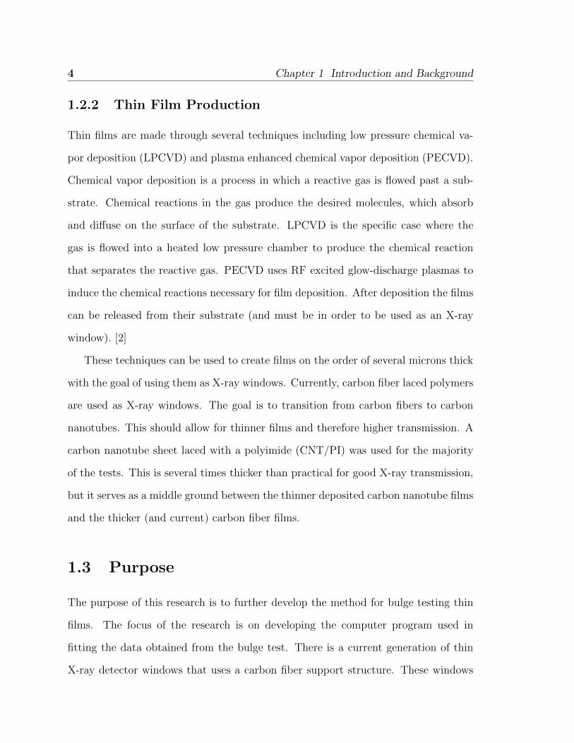
1.2.2 Thin Film Production

Thin films are made through several techniques including low pressure chemical va-

por deposition (LPCVD) and plasma enhanced chemical vapor deposition (PECVD).

Chemical vapor deposition is a process in which a reactive gas is flowed past a sub-

strate. Chemical reactions in the gas produce the desired molecules, which absorb

and diffuse on the surface of the substrate. LPCVD is the specific case where the

gas is flowed into a heated low pressure chamber to produce the chemical reaction

that separates the reactive gas. PECVD uses RF excited glow-discharge plasmas to

induce the chemical reactions necessary for film deposition. After deposition the films

can be released from their substrate (and must be in order to be used as an X-ray

window). [2]

These techniques can be used to create films on the order of several microns thick

with the goal of using them as X-ray windows. Currently, carbon fiber laced polymers

are used as X-ray windows. The goal is to transition from carbon fibers to carbon

nanotubes. This should allow for thinner films and therefore higher transmission. A

carbon nanotube sheet laced with a polyimide (CNT/PI) was used for the majority

of the tests. This is several times thicker than practical for good X-ray transmission,

but it serves as a middle ground between the thinner deposited carbon nanotube films

and the thicker (and current) carbon fiber films.

1.3 Purpose

The purpose of this research is to further develop the method for bulge testing thin

films. The focus of the research is on developing the computer program used in

fitting the data obtained from the bulge test. There is a current generation of thin

X-ray detector windows that uses a carbon fiber support structure. These windows

1.3 Purpose 5

are strong but not very thin. It is believed that by using carbon nanotubes as the

support structure the windows can be made much thinner. Though much research

needs to be done on the development of these new films, the purpose of this research

is to develop the method that will be used in characterizing future films.


Chapter 2

Methods and Materials

2.1 Materials

The films tested were carbon nanotube polyimide infused sheets (CNT/PI) and alu-

minum foil. The CNT/PI sheets were used as a proof of concept. Current X-ray

windows have a carbon fiber based support structure. This does not allow for films

much thinner than about 100 µm. The thickness of a film with grown carbon nan-

otubes could be less than one micron. The CNT/PI sheets used in this experiment

were about 30 µm thick. They were not grown for the purpose of this experiment. As

such they are much too thick for use in an X-ray window, but they serve as a proof

of concept for future development of CNT X-ray windows. To develop the CNT/PI

material a team took carbon nanotube paper (often called buckypaper) clamped be-

tween two 2” copper gaskets to prevent wrinkles and soaked it in a polyimide solution.

It was then baked to remove excess solution, hotpressed, and fully cured.

Aluminum foil was used as a cheaper and faster way to determine if the method

was working properly. The foil had a thickness of about 20 µm, comparable to that

of the CNT/PI. Sample preparation for the aluminum foil was much simpler. A piece

7

8 Chapter 2 Methods and Materials

Figure 2.1 This image is of CNT/PI at 20x magnification. It is difficult todetermine when it is in focus, which contributes to the uncertainty.

of standard vacuum grade aluminum foil was flattened by rolling to remove wrinkles.

It was then cut to size for either the bulge test or the pull test.

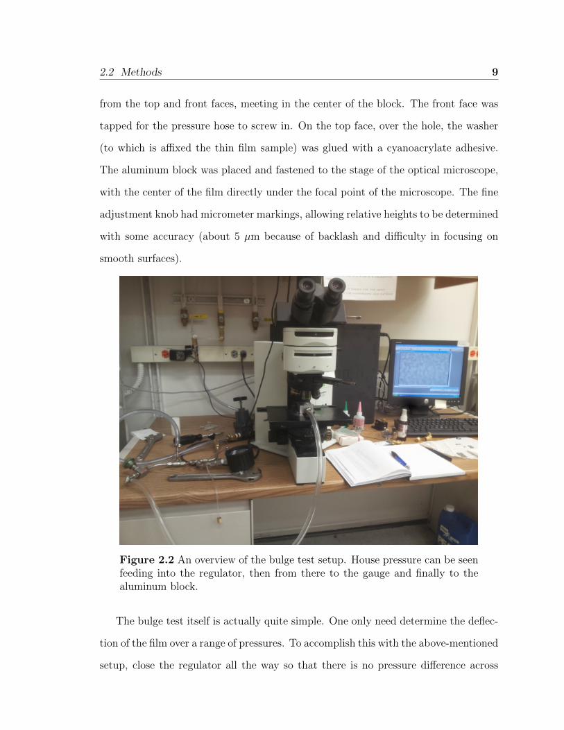
2.2 Methods

The basic bulge testing setup used in this experiment consisted of a pressure regulator,

an electronic pressure gauge, an aluminum stage, and an optical microscope. The

pressure regulator was connected to house pressure source with a maximum pressure

of 100 PSI. The regulator’s range was from 0-65 PSI (about 450 kPa). The pressure

gauge was placed immediately following the regulator. This gauge had an electronic

readout in units of kPa. With care, it was possible to adjust the pressure regulator

to the nearest kPa. Between the gauge and the aluminum stage was a pressure

release valve. The aluminum stage was approximately 1”x2”x3”. Holes were drilled

2.2 Methods 9

from the top and front faces, meeting in the center of the block. The front face was

tapped for the pressure hose to screw in. On the top face, over the hole, the washer

(to which is affixed the thin film sample) was glued with a cyanoacrylate adhesive.

The aluminum block was placed and fastened to the stage of the optical microscope,

with the center of the film directly under the focal point of the microscope. The fine

adjustment knob had micrometer markings, allowing relative heights to be determined

with some accuracy (about 5 µm because of backlash and difficulty in focusing on

smooth surfaces).

Figure 2.2 An overview of the bulge test setup. House pressure can be seenfeeding into the regulator, then from there to the gauge and finally to thealuminum block.

The bulge test itself is actually quite simple. One only need determine the deflec-

tion of the film over a range of pressures. To accomplish this with the above-mentioned

setup, close the regulator all the way so that there is no pressure difference across


Figure 2.3 A close up of the aluminum stage.

the film. Find and focus on the center of the film using the microscope’s stage and

focal adjustment dials. This part is actually rather difficult and is one of the larger

sources of error introduced by the setup. Data collection can begin once the center of

the film is in focus. To start, first record the current number on the fine adjustment

knob (in microns) for 0 kPa. Turning the regulator knob very carefully, increase the

pressure to 1 kPa. If the film has deflected, find the new focus and record the number

of the fine adjustment knob. It is important to know which way to turn the knob and

to not pass the new focus. Turning the adjustment knob in the opposite direction

introduces significant backlash. Sometimes the stiffness of the film is such that 1 kPa

does not cause a large enough deflection to be noticed visually. This is another source

of error introduced by this specific bulge test setup. Once both data are recorded,

increase the pressure again and record the deflection. If the film is not deflecting very

2.3 Error Analysis 11

rapidly, increase the step size. Often times a step size of 10 kPa or 20 kPa is needed in

order to cover the range of the pressure regulator for strong films that do not burst.

Continue this process until the film bursts, the desired pressure is reached, or the

regulator’s limit is reached. After the data are collected, a MATLAB fitting program

can be used to fit this data to the bulge test model, to find Young’s modulus (see

Appendix A). Figure 2.1 shows an example typical of the surfaces that were studied.

It is very difficult to find the focal plane, because of the relative smoothness of the

surface.

Sample preparation for the bulge test was accomplished by gluing (with an epoxy)

the sample of either aluminum foil or CNT/PI in between two washers. Two washers

were used to prevent wrinkles. If the film has wrinkles in it the bulge test equation

does not accurately describe its deflection. After preparation, the washer can be

affixed with a cyanoacrylate glue to the top of the aluminum stage. Cyanoacrylate

glue was used because there are readily available hardeners and release agents for

decreasing curing and sample removal time. The release agents were necessary for

the removal of the washer and the reuse of the aluminum block. Care was taken when

using the release agents, so as to not damage the film.

2.3 Error Analysis

Error analysis was a large part of the purpose of this research, which was to develop

a method for the characterization and comparison of the films. It was previously

mentioned that the two significant sources of error were in finding the center of the

film and in determining the relative height of the film at each deflection point. There

is no measured or calculated uncertainty in how far off the center is (which is perhaps

an improvement that can be made on this model). Most of the measured uncertainty


is in the x direction (height). MATLAB’s fitting functions take into account weights,

or uncertainties, but only in y (pressure). The transformation of the uncertainty of x

into the uncertainty in y is straight forward [4]. First, find the uncertainty in y that

comes from x (called δyI),

δyI = δxdy

dx.

Next, combine this with the measured (direct) uncertainty in y (called δyD),

δ2y = δ2yI + δ2yD.

Uncertainties also exist in the other measured values (radius and thickness) and in

the guess for Poisson’s ratio. These errors are propagated after the fitting is performed

and the parameters found. The function actually fit in MATLAB is

P = (c+ x)(a(c+ x)2 + b), (2.1)

where a = 83Y t/r2, b = 4tσi/r

2, and c = hi. The MATLAB fitting function returns

the calculated parameters along with their standard error. Solving for the desired

variables yields

Ycalc =3

8ar4/t (2.2)

and

σi =1

4br2/t.

This means that the uncertainty in Ycalc is

δY 2calc = (

∂Y

∂rδr)2 + (

∂Y

∂tδt)2 + (

∂Y

∂aδa)2

and likewise for the uncertainty in σi. Small and Nix [3] suggest that the value of Y

calculated from Eq. 2.2 can be made more accurate. Their suggestion is to pass Ycalc

through

Y =Ycalc

1 − 0.24ν − 0.00027(1 − ν)σi, (2.3)

2.4 Pull Test 13

where ν is the guess at Poisson’s ratio. The error is propagated through this equation,

just as above. Doing this gives Young’s modulus, intrinsic stress, and their associated

uncertainties.

2.4 Pull Test

Another mechanical tests exists for determining Young’s modulus, called the pull

test. In this test a strip of material is pulled by a machine that records force and

extension (how far it stretches). The slope of the force (load) versus extension graph

is Young’s modulus. This method offers one main advantage. It is fundamentally less

complicated than bulge testing, allowing for easier error propagation and (possibly)

more accurate measurement of Young’s modulus. The reason this test is not used

exclusively is because the bulge test is nearly identical to the application. An X-ray

window is circular (just like the sample in the circular washers) and it undergoes a

pressure differential in the same direction as the bulge test. The results of the pull

test are useful, though, in determining the accuracy of the bulge test itself.


Chapter 3

Results

3.1 Experimental Results

Approximately 30 bulge tests were performed during the course of this research.

The purpose of this research was to develop a method for testing thin film x-ray

windows to determine certain properties, like Young’s modulus. The method was to

include techniques for sample preparation, bulge testing and recording of the data, and

analysis of the data. Many of the tests were performed during the development of the

method, which make the data obtained therefrom less useful. (The data were useful

in developing the fitting program, but not in determining Young’s modulus.) Some of

the samples failed at low pressures because of improper preparation (discussed briefly

in the next paragraph). Other tests are not useful because they were performed on

a sample that had previously been tested. Once a sample deforms plastically, the

deflection data of any subsequent tests cannot be used to determine Young’s modulus

using the bulge equation. These samples were tested again as a means to practice

data collection and to refine the method. One sample is particularly relevant,though,

because the Young’s modulus obtained from bulge testing was very close to that

15

16 Chapter 3 Results

obtained from its pull test.

The sample was a CNT/PI sheet that had been fully cured at 400℃ (in previous

tests the CNT/PI samples had been cured at a lower temperature). This sample was

cut into enough pieces to perform three bulge tests and two pull tests. The bulge

test for the first sample was successfully performed. The two other samples failed

prematurely. For sample 2, the epoxy between the washers came undone at about

35 kPa. This most likely occurred because the washers were not properly cleaned

beforehand. These particular washers had some type of coating on them that needed

to be removed by sanding. Sample 3 failed in a similar manner at approximately

130 kPa. Upon inspection, it was observed that the sheet had split in two (like

separating two pieces of paper, not like tearing a piece of paper in half). One layer

was approximately 11 µm thick, the other 25 µm. This does not add up to the original

30 µm, but that is probably because the tear was uneven and two non-aligning parts

were measured. In addition to this, the measurement might have included some epoxy

from around the ring where the washer was affixed.

The results of the fully cured CNT/PI sample that survived its test were compared

to the results of the pull test. The sample was approximately 30 µm thick, affixed to

a washer of diameter 7.20 mm. The sample survived up to 400 kPa, which is about

the limit of the pressure regulator. A plot of pressure versus deflection can be seen

in Figure 3.1. This figure shows the deflection over only a portion of the range. One

can easily see how well the model (the line labeled “Fit”) fits the data in this region.

From this fit we find that Young’s modulus is about 3590 ± 160 MPa. The pull test

data for this sample can be seen in Figure 3.2. The average of Young’s modulus for

these two tests is about 3.45 GPa. The pull test is used as a comparison because it

is assumed to be inherently more accurate due to its simplicity.

There is a range of deflection during the bulge test where the model does not fit

3.2 MATLAB Fitting Program 17

the data very well. Generally, this is at the low deflection region. Figure 3.3 shows

the entire range for the same sample as Figure 3.1. As can be easily observed, the

model does not fit the data over the entire range very well.

These results are typical of other bulge tests. Figure 3.4 shows the data for a

CNT/PI sample that was not fully cured. Figure 3.5 shows that same sample where

the low deflection points are discarded. Ignoring these points is justified because of

the assumption of the bulge test that the deflection must be much greater than the

thickness of the film.

3.2 MATLAB Fitting Program

As discussed previously, the purpose of this research was to develop a method for

determining Young’s modulus. At this stage of the research, the method was much

more important than any of the specific results obtained thus far. The most important

part of the method that was developed as part of this research was the MATLAB

program used to fit the data. This program is listed in Appendix A. This program will

allow future research to focus on developing other parts of the method and eventually

on bulge testing thin films to obtain actual results.

The program uses MATLAB’s NonLinearModel.fit() function. This function

was chosen because of the way it returns the results of the fit. Namely, the individual

uncertainties in each parameter are returned. It also allows for the passing in of

weights, which are the experimental uncertainties.

Extensive care has been taken in commenting the code, but perhaps one more

item should be explained. The data parsing function, readData() expects the units

of the items in the data file to be in microns and kilopascals. This is convenient

because those are the units used during measurement. However, the units for pressure


are converted to megapascals to avoid errors in precision associated with doing the

computations in pascals and meters. This is possible because the units of length are

left in microns.

3.3 Discussion

The purpose of this research was to develop the method for bulge testing. As such, the

data obtained from any actual tests was not of very high priority. The real results

were in the MATLAB program, specifically in error propagation and data fitting.

The other parts of the methods, such as the process for bulge testing or sample

preparation, were important to refine for this stage of the research. However, as

the method evolves into being more automated, both of these processes will change.

The data fitting program will continue to be useful, though, as bulge test data is

fundamentally just pressure and displacement.

3.3 Discussion 19

−50 0 50 100 150 200 250 3000

0.05

0.1

0.15

0.2

0.25

0.3

0.35

0.4

0.45

Y = 3592.0867+/−158.6449 MPa

σ0 = 120.8201+/−0.6513 MPa

R2 = 0.99975

(Nix and Small) Nonlinear Fit

Deflection (µm)

Pre

ssure

(M

Pa)

Fit

Upper Conf.

Lower Conf.

Error

Data

Figure 3.1 The results of one bulge test of fully cured CNT/PI with thefitted line plotted to show how well the model fits this data. This plot doesnot include all of the data for the test. The first 21 data points are ignoredbecause they are in the low deflection limit, meaning they do not satisfydeflection >> thickness. Same sample as Figure 3.3.


0 0.2 0.4 0.6 0.8 1 1.2 1.4 1.6 1.8 2

0

5

10

15

20

Extension (mm)

Lo

ad

(N

)

Extension vs Load

Y1 = 3.3634 GPa

Y2 = 3.5395 GPa

Sample 1

Slope 1

Sample 2

Slope 2

Figure 3.2 The results of the pull test on two samples of fully cured CNT/PI.The slope of the force versus extension plot is Young’s modulus.

−50 0 50 100 150 200 250 300 350 400−0.1

0

0.1

0.2

0.3

0.4

0.5

0.6

Y = 16440.5719+/−2011.2332 MPa

σ0 = 40.3476+/−NaN MPa

R2 = 0.97723


Deflection (µm)

Pre

ssure

(M

Pa)

Fit

Upper Conf.

Lower Conf.

Error

Data

Figure 3.3 The results of one bulge test with the fitted line plotted to showthat the model does not fit the data very well. The sample is CNT/PI thatwas fully cured. Same as Figure 3.1.

3.3 Discussion 21

−100 0 100 200 300 400 500 600 700 800−0.1

0

0.1

0.2

0.3

0.4

0.5

0.6

Y = 6281.4758+/−584.813 MPa

σ0 = 209.1033+/−2.315 MPa

R2 = 0.99822


Deflection (µm)

Pre

ssure

(M

Pa)

Fit

Upper Conf.

Lower Conf.

Error

Data

Figure 3.4 This is a CNT/PI sample that was not fully cured. The modeldoes not fit the data over the entire region very well. There is no correspond-ing pull test data for this sample.


−100 0 100 200 300 400 500 6000

0.05

0.1

0.15

0.2

0.25

0.3

0.35

0.4

0.45

0.5

Y = 4726.6512+/−263.1254 MPa

σ0 = 234.5029+/−1.5788 MPa

R2 = 0.99958


Deflection (µm)

Pre

ssure

(M

Pa)

Fit

Upper Conf.

Lower Conf.

Error

Data

Figure 3.5 This is the same sample as in Figure 3.4. The model fits thedata much better over the region that discards the low deflection points.

Chapter 4

Conclusion

4.1 Conclusion

The purpose of this research was to develop a method for determining certain material

properties of thin films. This development focused on being able to programmatically

determine Young’s modulus from bulge test data. In addition to the development of

this a program to fit the data, the bulge test method was used to characterize several

samples of thin polyimide infused carbon nanotube sheets. In one such bulge test,

the Young’s modulus matched that of the pull test to within 5%. Unfortunately, the

other tests could not be correlated with pull test data because of sample failures.

Even though the results could not be verified, it is assumed that the fitting pro-

gram accurately performs the calculations to determine Young’s modulus, because

the same model has been used by previous researchers [3]. With this in mind, it can

also be assumed that any errors in the results are from errors in the data due to the

current system’s inaccuracies. These inaccuracies will be addressed in future work.

The fitting program itself is designed to be modular and modifiable. If the model

does need to be changed, it is as simple as modifying several lines in one function.

23

24 Chapter 4 Conclusion

4.2 Future Work

The bulge test equation makes the assumptions that the film is thin, the deflection is

greater than the thickness, and the bulge is spherical. It is easy to check and verify

that the samples adhere to the first two assumptions. The third, that the bulge is

spherical, is not addressed in this research. Future work for the team conducting

this research includes building an automated bulge test system that uses a laser

triangulation measuring device to determine deflection of the film. By using this

device, the team will be able to more accurately determine the true bulge shape of a

thin film under a pressure differential. This will be very useful. It has been shown

that the low deflection limit is not a spherical bulge, and thus is not accounted for

under the current model. A model that is accurate at these limits will allow for the

testing of films that do not deflect very much (either because they are weak and burst

too soon, or becase they are very stiff).

The new bulge test system will also address several large sources of error in the

current setup. The new system will be able to accurately find the center of the bulge,

measure the displacement, and measure the radius. These are inherently the largest

sources of error with the current system. This system is currently under development

at BYU.

An interesting question that should be asked is, “How does the support structure

affect the measurement of Young’s modulus?” The samples that were tested had

a support structure made of carbon nanotubes. The Young’s modulus of carbon

nanotubes is vastly different than that of the polymer. The current model seems to

work for such a compound film, but is there a more accurate model?

Bibliography

[1] D. R. Huston, W. Sauter, P. S. Bunt, B. Esser. ”Bulge testing of single-and dual-

layer thin films,” 26th Annual International Symposium on Microlithography.

(International Society for Optics and Photonics, 2001).

[2] M. Ohring. Materials science of thin films. (Academic Press, 2002), p. 716.

[3] M. K. Small, W. D. Nix. ”Analysis of the accuracy of the bulge test in deter-

mining the mechanical properties of thin films,” J. Mater. Res., Vol. 7 (No. 6),

1553-1563. (1992).

[4] P. R. Bevington, D. K. Robinson, Data reduction and error analysis for the

physical sciences. (McGraw Hill, New York, 2003), p. 102.

25

26 BIBLIOGRAPHY

Appendix A

MATLAB Fitting Program

The following is the MATLAB code in its entirety, used for determining Young’smodulus from a set of pressure and deflection data.

Listing A.1 Fitting code bulgetest nlm.m% Bulge t e s t data f i t t i n g program% In s t r u c t i o n s : Create a data f i l e with p r e s su r e and he ight data , accord ing% to the c o r r e c t format . Run t h i s program , s e l e c t the data f i l e , and% enjoy . You might get b e t t e r r e s u l t s by ad ju s t i ng the ' s t a r t ' and ' l a s t '% around l i n e 80 so that you can s e l e c t the most we l l behaved data . In% other words , the data that a c tua l l y d e s c r i b e s a s ph e r i c a l bulge .% ( See the comments above the readData ( ) func t i on on the data% f i l e format )% Author : Kyle Larsen ( lar11026@byui . edu )% Date : Summer 2013func t i on bulgetest_nlm

c l c ; c l e a r a l l ; c l o s e a l l ;% Suppress semi−co lon warning so we can pr in t in peace%#ok<∗NOPRT>

% See comment be f o r e ' readData ' f o r s t r u c tu r e o f data f i l e[ filename , pathname ] = u i g e t f i l e ( ' ∗ . csv ' , 'DefaultName ' , ' data/ ' ) ;

% I f cance l i s pressed , e x i ti f isequal ( filename , 0)

r e turnend

% Concatenate the path and f i l e namesdata_file = [ pathname , filename ] ;

% Read in the va lue sdata = readData ( data_file ) ;

% Assign data to v a r i a b l e sr = data (1 , 1) ; % Radius o f washert = data (1 , 2) ; % Thickness o f f i lmv = data (2 , 1) ; % Guess at Poisson ' s r a t i o

27

28 Chapter A MATLAB Fitting Program

% Get the s t a r t po int from the data f i l e , e l s e d e f au l t to some va lues .startPoint = [ data (3 , 1) data (3 , 2) data (3 , 3) ] ;

% Since we want to s t o r e the s t a r t po int in f am i l i a r uni t s , i t must be% transformed here in to what the f i t t i n g func t i on expect s .startPoint = [8∗ t∗startPoint (1 ) /(3∗ r ˆ4) 4∗t∗startPoint (2 ) /rˆ2 startPoint (3 ) ] ;

% I f the s t a r t po in t s aren ' t set , s e t a d e f au l ti f ˜ isempty ( startPoint ( startPoint == 0) )

startPoint = [1000 100 1 ] ;end

left = 11 ;right = length ( data ) − 3 ;% The un i t s used in t h i s program are MPa and microns . Matlab does not% have enough p r e c i s i o n to perform the f i t t i n g s with Pasca l s and% meters ( f o r some reason ) .y = data(3+left :3+right , 1) . / 1000 ;x = data(3+left :3+right , 2) ;

% Errorssyd = data(3+left :3+right , 3) . / 1000 ; % Direc t e r r o r in ysx = data(3+left :3+right , 4) ; % Direc t e r r o r in xsv = data (2 , 2) ; % Estimated e r r o r in Poisson ' s r a t i osr = data (1 , 3) ; % Error in rad iu sst = data (1 , 4) ; % Error in th i c kne s s

% Our s i g n i f i c a n t e r r o r i s in the x va r i ab l e ( d i sp lacement ) .% Bevington d e s c r i b e s a method on pg 102 o f Data Reduction and Error% Analys i s f o r Phys i ca l S c i enc e s that a l l ows the e r r o r in x to be% combined with the e r r o r in y .dx = d i f f ( x ) ;dx ( dx == 0) = eps ; % Replace a l l 0 s to avoid div−by−zeroslope = ( d i f f ( y ) . / dx ) ;

% Repeat l a s t row to get c o r r e c t number o f rowsslope = [ slope ; slope ( end ) ] ;

% Ind i r e c t e r r o r in ysyi = sx .∗ slope ;

% Combined e r r o rsy = sqr t ( syi . ˆ2 + syd . ˆ 2 ) ;

% Limit the area we analyze . This he lp s po s s i b l y because e a r l i e r data% po in t s don ' t d e s c r i b e a s ph e r i c a l bulgestart = 1 ;last = length ( x ) ;x = x ( start : last ) ;y = y ( start : last ) ;sy = sy ( start : last ) ;sx = sx ( start : last ) ;

% Subtract the min so that d e f l e c t i o n s t a r t s at ze ro .x = x − min( x ) ;

mdl = nlm_bulge (x , y , sx , sy , r , t , v , sr , st , sv , startPoint ) ;end

func t i on mdl = nlm_bulge (x , y , sx , sy , r , t , v , sr , st , sv , startPoint )% Create the model func t i on as an anonymous func t i on .% 'b ' i s a vec to r conta in ing a l l o f the parameters ( three in t h i s case )modelfun = @ (b , x ) ( ( b (3 ) + x ( : , 1) ) . ∗ ( b (1 ) . ∗ ( b (3 ) + x ( : , 1) ) .ˆ2+b (2 ) ) ) ;

29

% One improvement i s to make these i n i t i a l gue s s e s more e a s i l y% ad ju s t ab l e .beta0 = startPoint ;mdl = NonLinearModel . fit (x , y , modelfun , beta0 , 'Weights ' , sy ) ;

% Cal l the parameters a , b , and c , to be more c on s i s t e n t with the other% f i t t i n g method . Except here we append 'p ' f o r parameter because a , b ,% and c are used below f o r the adjusted parameters .% Set easy ac c e s s f o r our parameterspa = mdl . Coefficients . Estimate (1 ) ;pb = mdl . Coefficients . Estimate (2 ) ;pc = mdl . Coefficients . Estimate (3 ) ;psa = mdl . Coefficients . SE (1 ) ;psb = mdl . Coefficients . SE (2 ) ;psc = mdl . Coefficients . SE (3 ) ;

% ' psc ' i s o f t en NaN ( not a number ) . I f that ' s the case , s e t i t to the% sma l l e s t number MATLAB knows .i f i snan ( psc )

psc = eps ;end

% Transform the parameters i n to Young ' s modulus and i n t r i n s i c s t r e s sa = 3∗r ˆ4/(8∗ t ) ∗pa ; % c a l l e d Ycalc in Nix and Small ' s paperb = r ˆ2/(4∗ t ) ∗pb ; % This i s sigma0c = pc ;

% This equat ion i s a l s o from the Nix and Small paper . See the paper% f o r the reason why t h i s i s more accurate .Y = a /(1 − 0 .24∗ v − 0 .00027∗ (1 − v ) ∗b ) ;sa = sqr t ( (3∗ r ˆ3/(2∗ t ) ∗pa∗sr ) ˆ2 + (−3∗r ˆ4/(8∗ t ˆ2) ∗pa∗st ) ˆ2 + (3∗ r ˆ4/(8∗ t ) ∗psa )←↩

ˆ2) ;sb = sqr t ( (1∗ r /(2∗ t ) ∗pb∗sr ) ˆ2 + (−r ˆ2/(4∗ t ˆ2) ∗pb∗st ) ˆ2 + ( r ˆ2/(4∗ t ) ∗psb ) ˆ2) ;sc = psc ;

% Propogate the e r r o r from the Y parameter to the modi f i ed YsY = sqr t ( sa ˆ 2 / (1 − 0 .24 ∗ v − 0 .27 e−3 ∗ (1 − v ) ∗ b ) ˆ 2 + Y ˆ 2 ∗ (−0.24←↩

+ 0.27 e−3 ∗ b ) ˆ 2 ∗ sv ˆ 2 / (1 − 0 .24 ∗ v − 0 .27 e−3 ∗ (1 − v ) ∗ b ) ˆ 4 +←↩Y ˆ 2 ∗ (−0.27e−3 + 0.27 e−3 ∗ v ) ˆ 2 ∗ sa ˆ 2 / (1 − 0 .24 ∗ v − 0 .27 e−3 ∗ ←↩

(1 − v ) ∗ b ) ˆ 4) ;

% Construct the l i n e a r l y spaced vec to r s used to c r e a t e the f i t t e d l i n e% and i t s con f idence i n t e r v a l .% Modif ied from :% http ://www. mathworks . com/help / s t a t s / examples /weighted−nonl inear−r e g r e s s i o n .←↩

htmlxx = l i n s p a c e ( x (1 ) , x ( end ) ) ' ;

% Plot f i t and upper and lower boundsp l o t ( xx , modelfun ( [ pa pb pc ] , xx ) , ' r− ' , xx , modelfun ( [ pa+psa pb+psb pc+psc ] , ←↩

xx ) , ' g : ' , xx , modelfun ( [ pa−psa pb−psb pc−psc ] , xx ) , ' g : ' ) ;hold on

% Plot the data with e r r o r bars f o r the x va r i ab l e . The e r r o r in y i s% too smal l to s ee .% http ://www. mathworks . com/mat labcentra l / f i l e e x chang e /22216− p l o t e r rploterr (x , y , sx , [ ] , 'b . ' ) ;

% Get the l im i t s so we can ac cu ra t e l y p lace the t ext on the graph .YLim = get ( gca , 'YLim ' ) ;XLim = get ( gca , 'XLim ' ) ;

% Pr int i n t e r e s t i n g i n f o s t r a i g h t on the graph .t ex t ( XLim (1 ) , YLim (2 )−YLim (2 ) /6 , [ 'Y = ' , num2str ( Y ) , '+/− ' , num2str ( sY ) , ' MPa←↩

' ] ) ;

30 Chapter A MATLAB Fitting Program

t ex t ( XLim (1 ) , YLim (2 )−YLim (2 ) /3 , [ ' \ s igma 0 = ' , num2str ( b ) , '+/− ' , num2str ( sb )←↩, ' MPa ' ] ) ;

t ex t ( XLim (1 ) , YLim (2 )−YLim (2 ) /2 , [ 'Rˆ2 = ' , num2str ( mdl . Rsquared . Adjusted ) ] ) ;

t i t l e ( ' (Nix and Small ) Nonl inear Fi t ' , ' FontSize ' , 14) ;x l ab e l ( ' De f l e c t i on (\mum) ' ) ;y l ab e l ( ' Pressure (MPa) ' ) ;l egend ( ' Fit ' , 'Upper Conf . ' , 'Lower Conf . ' , ' Error ' , 'Data ' , ' Locat ion ' , '←↩

SouthEast ' )

f p r i n t f ( 'Nix and Small (Non l i n e a r ) \n−−−−−−−−−−−−−−−\nY = %g+/−%g MPa; sigma0 =←↩%g+/−%g MPa; h i = %g\n ' , Y , sY , b , sb , pc ) ;

end

% The data s t r u c tu r e now in c l ud e s the radius , th i cknes s , and% guess f o r Poisson ' s r a t i o and t h e i r a s s o c i a t ed e r r o r s . Add i t i ona l ly , the% i n i t i a l gue s s e s at the parameters are inc luded ( but a d e f au l t i s supp l i ed% in the code , i f l e f t 0 .

% The data f i l e i s a comma seperated value f i l e . There are 4% columns . The f i r s t two rows conta in the radius , th i cknes s , and% Poisson ' s r a t i o guess ( a long with t h e i r e r r o s and some unused s l o t s ) .% The th i rd row conta in s the gue s s e s at the i n i t i a l parameters .% The format i s as f o l l ow s :% RADIUS,THICKNESS,ERROR R,ERROR T% POISSON,ERROR POIS,UNUSED,UNUSED% START A,START B,START C,UNUSED% PRESSURE,HEIGHT,ERROR P,ERRORH% PRESSURE,HEIGHT,ERROR P,ERRORH% PRESSURE,HEIGHT,ERROR P,ERRORH% etc , etc , etc , e t c

func t i on data = readData ( data_file )data = dlmread ( data_file ) ;

end

Documents

SPHERICAL BULGE TESTING OF THIN FILM X-RAY WINDOWS by …