Speed Limits Set Lower Than Engineering …...SPEED LIMITS SET LOWER THAN ENGINEERING RECOMMENDATIONS Final Report Prepared by: Eric T. Donnell Professor Vikash V. Gayah Assistant

SPEED LIMITS SET LOWER THAN ENGINEERING RECOMMENDATIONS

Final Reportprepared forTHE STATE OF MONTANADEPARTMENT OF TRANSPORTATION

in cooperation withTHE U.S. DEPARTMENT OF TRANSPORTATIONFEDERAL HIGHWAY ADMINISTRATION

August 2016prepared byEric T. DonnellVikash V. Gayah

Zhengyao YuLingyu LiAnthony DePrator

The Thomas D. Larson Pennsylvania Transportation Institute-Pennsylvania State UniversityState College, PA

FHWA/MT-16-008/8225-001

R E S E A R C H P R O G R A M S

You are free to copy, distribute, display, and perform the work; make derivative works; make commercial use of the work under the condition that you give the original author

and sponsor credit. For any reuse or distribution, you must make clear to others the license terms of this work. Any of these conditions can be waived if you get permission from the sponsor. Your fair use and other rights are in no way affected by the above.

SPEED LIMITS SET LOWER THAN ENGINEERING RECOMMENDATIONS

Final Report

Prepared by:

Eric T. Donnell Professor

Vikash V. Gayah Assistant Professor

Zhengyao Yu, Lingyu Li, Anthony DePrator Graduate Research Assistants

The Thomas D. Larson Pennsylvania Transportation Institute Pennsylvania State University

201 Transportation Research Building University Park, PA 16802

Prepared for:Montana Department of Transportation

August 2016

Technical Report Documentation Page

1. Report No.FHWA/MT-16-008/8225-01

2. Government Accession No. 3. Recipient’s Catalog No.

4. Title and SubtitleSpeed Limits Set Lower than Engineering Recommendations

5. Report DateAugust 2016

6. Performing Organization Code

7. Author(s)Eric T. Donnell, Vikash G. Gayah, Zhengyao Yu, Lingyu Li, and AnthonyDePrator

8. Performing Organization Report No.

LTI Report No. 2017-02

9. Performing Organization Name and AddressThe Thomas D. Larson Pennsylvania Transportation InstituteThe Pennsylvania State University201 Transportation Research BuildingUniversity Park, PA 16802

10. Work Unit No. (TRAIS)

11. Contract or Grant No.MDT Contract 8225-001

12. Sponsoring Agency Name and AddressResearch ProgramsMontana Department of Transportation (SPR)http://dx.doi.org/10.13039/1000092092701 Prospect AvenuePO Box 201001

13. Type of Report and Period CoveredFinal Report: September 2014 – August 2016

14. Sponsoring Agency Code5401

15. Supplementary NotesConducted in cooperation with the U.S. Department of Transportation, Federal Highway Administration. This report can be found athttp://www.mdt.mt.gov/research/projects/traffic/speed_limits_lower.shtml

16. AbstractThe purpose of this project is to provide the Montana Department of Transportation (MDT) with a better understanding of theoperational and safety impacts of setting posted speed limits below engineering recommended values. This practice has beenperformed on Montana roadways for a variety of reasons but the safety and operational impacts are largely unknown. An EmpiricalBayes observational before-after study found that there is a statistically significant reduction in total and fatal and injury crashes atsites with engineering speed limits set 5 mph lower than engineering recommendations. At locations with posted speed limits set10 mph lower than engineering recommendations, there was a decrease in total crash frequency, but an increase in fatal and injurycrash frequency. The safety effects of setting posted speed limits 15 or 25 mph lower than engineering recommendations is lessclear, because the results were not statistically significant, due to the small sample size of sites available for inclusion in theanalysis. An operating speed evaluation found that, when the posted speed limit was set only 5 mph lower than the engineeringposted speed limit, drivers tend to more closely comply with the posted speed limit. Compliance tends to lessen as the differencebetween the engineering recommended posted speed limit and the posted speed limit increases. The practice of light enforcement,which was defined as highway patrol vehicles making frequent passes through locations with posted speed limits set lower thanengineering recommendations, appeared to have only a nominal effect on vehicle operating speeds. Known heavy enforcement,defined as a stationary highway patrol vehicle present within the speed zone, reduced mean and 85 th-percentile vehicle operatingspeeds by approximately 4 mph.

17. Key Words85th percentile speed, Behavior, Best practices, Crash data, Data collection,Design, Design speed, Geometric design, Highway safety, Literature review,Operating speed, Speed, Speed Control, Speed signs, Speeding, Trafficcontrol, Traffic control devices, Traffic law enforcement, Traffic safety, Trafficsigns, Traffic speed, Travel behavior, Speed limits, Safety, Empirical Bayes,Enforcement

18. Distribution StatementNo restrictions. This document is availablefrom the National Technical Information Service,Springfield, VA 22161

19. Security Classif. (of this report)

Unclassified

20. Security Classif. (of this page)

Unclassified

21. No. of Pages

102

22. Price

N/A

http://www.mdt.mt.gov/research/projects/traffic/speed_limits_lower.shtml

iii

Disclaimer Statement This document is disseminated under the sponsorship of the Montana Department of Transportation (MDT) and the United States Department of Transportation (USDOT) in the interest of information exchange. The State of Montana and the United States assume no liability for the use or misuse of its contents.

The contents of this document reflect the views of the authors, who are solely responsible for the facts and accuracy of the data presented herein. The contents do not necessarily reflect the views or official policies of MDT or the USDOT.

The State of Montana and the United States do not endorse products of manufacturers.

This document does not constitute a standard, specification, policy or regulation.

MDT attempts to provide accommodations for any known disability that may interfere with a person participating in any service, program, or activity of the Department. Alternative accessible formats of this information will be provided upon request. For further information, call 406/444.7693, TTY 800/335.7592, or Montana Relay at 711.

iv

v

TABLE OF CONTENTS Table of Contents ............................................................................................................................ v

List of Tables ................................................................................................................................ vii

List of Figures .............................................................................................................................. viii

Introduction and Background ......................................................................................................... 1

Review of Existing Literature ......................................................................................................... 5

Speed ........................................................................................................................................... 5

Posted Speed Limits ................................................................................................................ 5

Design Speed .......................................................................................................................... 6

Operating Speeds .................................................................................................................... 7

State Practices for Setting Posted Speed Limits ................................................................... 15

Conflicting Design Speeds and Speed Limits ....................................................................... 16

Speed Limit Compliance and Enforcement .............................................................................. 20

Speed Choice and Compliance ............................................................................................. 21

Enforcement .......................................................................................................................... 21

Speed and Safety ....................................................................................................................... 25

Speed and Crash Severity ..................................................................................................... 29

Speed Enforcement and Safety ............................................................................................. 30

Summary of Findings ................................................................................................................ 31

Survey of Agency Practices .......................................................................................................... 33

Results ....................................................................................................................................... 35

Notable practices ................................................................................................................... 36

Summary of Findings ................................................................................................................ 37

Data Collection ............................................................................................................................. 39

Speed Data ................................................................................................................................ 39

Data Collection Procedures ................................................................................................... 39

Data Compilation Process ..................................................................................................... 42

Crash Data ................................................................................................................................. 43

Analysis Methodology .................................................................................................................. 46

Operating Speed Analysis ......................................................................................................... 46

Appropriateness of Sample Size ........................................................................................... 46

Comparison of Speed Variances ........................................................................................... 47

vi

Comparison of Speed Proportions ........................................................................................ 47

Modeling Operating Speeds .................................................................................................. 48

Safety Analysis ......................................................................................................................... 50

Step 1 – Prediction of Future Safety Performance ................................................................ 51

Step 2 – Before-After Analysis with Empirical Bayes ......................................................... 52

Step 3 – Compare Predicted and Actual Safety Performance ............................................... 53

Results ........................................................................................................................................... 54

Operating Speed Analysis ......................................................................................................... 54

Summary Statistics of Speed Data ........................................................................................ 54

Models of Operating Speeds and Speed Limit Compliance ................................................. 62

Safety Analysis ......................................................................................................................... 68

Summary Statistics of Crash Data ........................................................................................ 68

Empirical-Bayes Before-After Analysis ................................................................................... 71

Step 1 – Prediction of Future Safety Performance ................................................................ 71

Step 2 – Before-After Analysis with Empirical Bayes ......................................................... 76

Step 3 – Crash Modification Factors .................................................................................... 77

Conclusions ................................................................................................................................... 79

References ..................................................................................................................................... 82

Appendix A: State Transportation Agency Survey .................................................................... A-1

Appendix B: Schematic drawings of speed detector locations ................................................... B-1

vii

LIST OF TABLES Table 1 – V85 Prediction Models for Two-Lane Rural Highways ............................................... 10 Table 2 – Speed Models Developed by Jessen et al. (2001) ......................................................... 12 Table 3 – Summary of Descriptive Statistics for Work Zone Speed Limit Compliance .............. 18 Table 4 – Designs of Speed Limit Enforcement Field Studies ..................................................... 22 Table 5 – Summary of Halo Effects ............................................................................................. 24 Table 6 – Power Model Coefficients from Meta-Analysis ........................................................... 27 Table 7 – Summary of Speed Related CMF Studies (FHWA 2014b) .......................................... 28 Table 8 – Odds Ratio of Injury by Severity and Study Sites Versus Comparison Sites............... 30 Table 10 – Details of Crash Data Available at Treated Sites ....................................................... 44 Table 11 – Details of Crash Data Available at Reference Sites ................................................... 45 Table 12 – Values for Speed Sample Size Determination ............................................................ 47 Table 13 – Summary Statistics For Observed Speeds During “No Enforcement” Period ........... 56 Table 14 – Summary Statistics for Observed Speeds During “Light Enforcement” Period ........ 58 Table 15 – Summary Statistics for Observed Speeds During “Heavy Enforcement” Period ....... 60 Table 16 – Summary Statistics for Operating Speed Data ........................................................... 63 Table 17. ANOVA Test Statistics For Operating Speeds ............................................................. 63 Table 18 – Linear Regression Modeling Output for Mean Operating Speeds ............................. 64 Table 19 – Quantile Regression Modeling Output for 85th Percentile Operating Speeds ............ 66 Table 20 – Logistic Regression Modeling Output for Speed Limit Compliance ......................... 67 Table 21 – Odds Ratios Associated with Logistic Regression Output ......................................... 68 Table 22 – Summary of Crash Frequency and Crash Rates for Treatment Sites ......................... 69 Table 23 – Summary of Crash Frequency and Crash Rates for Reference Sites .......................... 70 Table 24 – Summary Statistics for 2-Lane Roadway Segments Used to Develop SPFs .............. 72 Table 25 – Summary Statistics for 4-Lane Roadway Segments Used to Develop SPFs .............. 73 Table 26 – Statistical Modeling Output for 2-lane Roadway Segments for Total Crash Frequency....................................................................................................................................................... 74 Table 27 – Statistical Modeling Output for 2-lane Roadway Segments for Fatal + Injury Crash Frequency ...................................................................................................................................... 74 Table 28 – Statistical Modeling Output for 4-lane Roadway Segments for Total Crash Frequency....................................................................................................................................................... 75 Table 29 – Statistical Modeling Output for 4-lane Roadway Segments for Fatal + Injury Crash Frequency ...................................................................................................................................... 75 Table 30 – Reported and Expected Crash Frequencies for Treatment Sites After Implementation of Lower Than Engineering Recommended Speed Limits ........................................................... 77 Table 31 – Crash Modification Factors for Implementation of Speed Limits Lower Than Engineering Recommended Values .............................................................................................. 77

viii

LIST OF FIGURES Figure 1 – Depiction of the Relationship Between Inferred Design Speed and Other Speeds ....... 7 Figure 2 – Crash Involvement as a Function of Speed for Daytime and Nighttime Crashes ....... 25 Figure 3 – CMF for Relative Speed Enforcement. ....................................................................... 31 Figure 4 – Flowchart Depicting the Structure of the Survey ........................................................ 34 Figure 5 – States of Which an Agency Representative was Contacted for the Survey ................ 35 Figure 6 – Data Collection Sites (Google 2015) ........................................................................... 40

1

EXECUTIVE SUMMARY The purpose of this project is to provide the Montana Department of Transportation (MDT) with objective information concerning the operational and safety impacts of setting posted speed limits lower than engineering recommended values. This practice has been used on Montana roadways for a variety of reasons, but the safety and operational impacts are largely unknown. The project involved four unique components: a comprehensive literature review, a survey of other state transportation agencies, collection of speed and safety data from a variety of Montana roadways, and an analysis of these data.

The literature review revealed that little published information exists on the practice of setting posted speed limits lower than engineering recommended values. The survey was sent to all state transportation agencies with representation on the AASHTO Subcommittee on Traffic Engineering, which included a total of 71 representatives from 51 states or territories. A total 22 of the 28 responding agencies indicated that they engaged in the practice of setting speed limits lower than engineering recommendations. About half of these agencies had a policy or guidance document describing the practice. Overall, few agencies reported evaluating the changes to operating speed or safety resulting from setting speed limits lower than engineering recommendations. About half of the 28 responding agencies evaluated driver compliance with the lower posted speed limit and found that the compliance was generally poor.

Operating speed data were collected at three sites with posted speed limits set 5 mph lower than engineering recommendations; two sites with posted speed limits set 10 mph lower than engineering recommendations; two sites with posted speed limits set 15 mph lower than engineering recommendations; one site with a posted speed limit set 25 mph lower than engineering recommendations; and, four comparison sites with posted speed limits set equal to the engineering recommended values. Data were collected from each site on three unique days: one with no speed enforcement present; one with light speed enforcement present; and, one with heavy speed enforcement present. Statistical models were developed to describe mean operating speeds, 85th percentile operating speeds and driver compliance with posted speed limits.

The operating speed evaluation produced results that were consistent with other state transportation agency experiences when setting posted speed limits lower than engineering recommendations. When the posted speed limit was set only 5 mph lower than the engineering posted speed limit, drivers tended to more closely comply with the posted speed limit. Compliance tended to lessen as the difference between the engineering recommended posted speed limit and the posted speed limit increased. When the posted speed limit was set 15 to 25 mph lower than the engineering recommended speed limit, there appeared to be a low level of compliance with the posted speed limit. The practice of light enforcement, which was defined as highway patrol vehicles making frequent passes through locations with posted speed limits set lower than engineering recommendations, appeared to have only a nominal effect on vehicle operating speeds. Known heavy enforcement, defined as a stationary highway patrol vehicle present within the speed zone, reduced mean and 85th-percentile vehicle operating speeds by

2

approximately 4 mph. Additionally, known heavy enforcement increased the odds that drivers would comply with the posted speed limit.

The safety evaluation included reported crash frequency data from six sites with posted speed limits set 5 mph lower than engineering recommendations; five sites with posted speed limits set 10 mph lower than engineering recommendations; two sites with posted speed limits set 15 mph lower than engineering recommendations; and, one site with a posted speed limit set 25 mph lower than engineering recommendations. The research team used the empirical Bayes (EB) before-after approach to develop Crash Modification Factors (CMFs) to describe the expected change in crash frequency when setting posted speed limits lower than engineering recommendations. The proposed EB analysis properly accounts for statistical factors such as: regression-to-the-mean, differences in traffic volume, and crash trends (time series effects) between the periods before and after posted speed limits were set lower than engineering recommendations.

While data were only available for a handful of sites that implemented this practice, the before-after analysis found that there is a statistically significant reduction in total and fatal + injury crashes at locations with posted speed limits set 5 mph lower than engineering recommendations. Locations with posted speed limits set 10 mph lower than engineering recommendations experienced a decrease in total crash frequency but an increase in fatal + injury crash frequency. The safety effects of setting speed limits 15 to 25 mph lower than engineering recommendations is less clear as the results were not statistically significant, likely due to the small sample of sites included in the evaluation.

3

INTRODUCTION AND BACKGROUND The Montana Department of Transportation (MDT) generally ensures that posted speed limits are set in accordance with engineering recommendations, which are typically set such that they are about equal to the observed 85th percentile operating speed. However, for a variety of reasons including the presence of school zones, citizen requests, political pressure, and perceived safety issues, posted speed limits on several roadways in Montana have been reduced to values lower than those recommended for the facility by engineering guidelines. However, engineers and decision-makers in the state do not have a good understanding of the operational and safety impacts of implementing speed limits lower than engineering recommendations. Limited field observations suggest that drivers generally do not comply with these lower speed limits, perhaps because the drivers are familiar with the original speed limits or the roadway environment (e.g., alignment and cross-section features) promotes operating speeds that exceed the posted speed limit. Anecdotal local evidence suggests that the presence of law enforcement at these locations may have a positive effect on speed limit compliance (i.e., driver compliance with the posted speed limits increases when police enforcement is present). However, the relationship between the intensity of police presence and compliance with the reduced posted speed limits is not well understood. Furthermore, the crash frequency and severity impacts of posting speed limits lower than engineering recommendations are not well understood.

This study examines the safety and operational effects of posting speed limits lower than engineering recommendations. With regards to safety, crash frequency and severity are considered. The mean, 85th-percentile, pace and speed limit compliance are assessed in the operational evaluation. Specifically, the objectives of this study are as follows:

Quantify the change in mean and 85th percentile vehicle operating speeds, pace and speed limit compliance at sites where posted speed limits are set lower than engineering recommendations for different magnitudes of posted speed limit reductions; Quantify the relationship between speed limit compliance and presence of police enforcement at sites where posted speed limits are set lower than engineering recommendations; and, Quantify the safety performance of roadway segments with posted speed limits set lower than engineering recommendations, measured by the frequency and severity of crashes.

These results will provide the Montana Department of Transportation (MDT) with the requisite information to make more informed decisions about the practice and application of setting posted speed limits lower than engineering recommendations and the minimum level of enforcement required to achieve given levels of speed limit compliance of these facilities.

The remainder of this report is organized into six sections. The first provides a review of the relevant literature on speed concepts, setting of posted speed limits, speed enforcement and safety. The second summarizes a survey of state transportation agency practices with respect to setting speed limits lower than engineering recommendations. The third section describes the data collection that was performed to obtain the operating speed and safety data used in the

4

present study. This is followed by a description of the methodology used to analyze these data. The fifth section provides a detailed discussion of the results, which is organized by operating speed and safety. Finally, the report concludes with a summary of the findings and recommendations to implement the results.

5

REVIEW OF EXISTING LITERATURE Current research regarding the safety and operational effects of setting speed limits lower than engineering recommendations is limited. To account for this limitation in the published literature, this review broadly considers the relationships between various speed measures and how these speed measures impact safety performance. The literature review begins with a discussion of speed concepts, including the relationship between posted speed limits, operating speeds, and design speeds. Issues related to speed compliance and enforcement are then described. The literature review concludes with a brief discussion of the effects of speed on safety.

SPEED This section of the report focuses on the posted speed limit, design speed, and operating speed. The speed limit is the maximum regulatory speed at which a vehicle can legally traverse a roadway. The design speed of a roadway is one of the controlling criteria for a roadway and is used directly and indirectly to establish the geometric features of the roadway (AASHTO 2011). The operating speed is defined as the speed at which vehicles are observed under free-flow conditions. The most common operating speed measure is the 85th percentile of the speed distribution. Each of these speed concepts is described in more detail below.

POSTED SPEED LIMITS Posted speed limits are conveyed by regulatory signs and are established in increments of five miles per hour (mph). The Federal Highway Administration’s (FHWA) SPEED CONCEPTS: INFORMATION GUIDE (Donnell et al. 2009) describes two methods for establishing posted speed limits: legislative/statutory and an engineering study. A statutory (or legislative) speed limit is established by law and often provides maximum posted speed limits based on specific roadway categories (e.g., local street or urban arterial). This method is often criticized for its arbitrary assignment of speed limits independent of site characteristics. Enforcement officials are challenged to manage operating speeds on roadways with statutory speed limits due to their arbitrary assignment (Transportation Research Board 1998).

An engineering study consists of collecting a sample of free-flow vehicle operating speeds, often under favorable conditions (e.g., daylight with no adverse weather conditions), and compiling a speed distribution. The 85th percentile speed of the sample data is most often used to establish the posted speed limit. Being that this speed limit is based on field data, the posted speed limit is much more reliable in identifying drivers travelling at excessive speeds. This process implies that only a limited proportion of vehicles (15 percent) will violate the posted speed limit. In practice, the number of speed limit violators is likely even fewer because enforcement officers typically provide a 5-10 mph allowance over the posted speed limit before offering traffic citations (Transportation Research Board 1998). Specific instructions for undertaking a spot speed study are laid out by the Institute of Transportation Engineers (ITE) in MANUAL OF TRANSPORTATION ENGINEERING STUDIES (Institute of Transportation Engineers 2010). Posted speed limits based

6

on the results of this study are often considered more rational than posted speed limits based on legislative policy.

The definition of a vehicle operating under “free-flow” conditions varies. Most studies classify a vehicle in free-flow conditions based on a minimum time headway. Hauer, Ahlin, and Bowser (1981) selected 4 seconds as the minimum headway value based on previous research, which indicated that drivers adjust speed at headways of less than 3 seconds (Ahlin 1979). Misaghi and Yassan (2005) considered vehicle headways of less than 5 seconds as non-free-flow. The Highway Capacity Manual procedure requires vehicles to have a leading headway of 8 seconds as well as a lagging (or following) headway of 5 seconds (Transportation Research Board 2010).

Two other, but less common, methods for setting speed limits are optimization and the expert system approach (Forbes et al. 2012). Optimization is an approach in which all “costs” associated with transportation (safety, travel time, fuel consumption, noise, and pollution) are considered and the speed limit is selected to minimize the total sum of these costs. The expert system approach utilizes a computer program with an extensive knowledge base to recommend a speed limit based on prior experience. A current example of the expert system approach is FHWA’s USLIMITS2, a tool for communities that lack access to engineers with experience in establishing speed limits. USLIMITS2 has been used in over 3,000 projects with users from a wide range of backgrounds (federal, state, local government, non-profits, consultants, and even law enforcement) (FHWA 2014a). Examples of specific uses of USLIMITS2 include: verifying the findings of an engineering speed study to increase a speed limit in Michigan; using site characteristics to determine if a speed limit should be reduced in Indiana; and, checking the validity of speed limits during a statewide safety analysis in Wisconsin (Warren, Xu, and Srinivasan 2013).

DESIGN SPEED The American Association of State Highway Transportation Officials’ (AASHTO) A POLICY ON GEOMETRIC DESIGN OF HIGHWAYS AND STREETS (AASHTO 2011), commonly referred to as the AASHTO GREEN BOOK, uses the design speed concept to produce design consistency. Using this concept, a design speed is selected for a roadway and then used as a direct or indirect input to establish many geometric design criteria, such as horizontal alignment, vertical alignment, sight distance, and cross-section elements.

The equations that provide design criteria based on the design speed are often conservative. This fact, combined with conservative decision-making in the design process, results in roadway environments that often encourage drivers to travel faster than the intended design speed. This results in an “inferred” design speed being communicated to the driver (Donnell et al. 2009) and operating speeds that are sometimes higher than the design speed of the roadway.

The inferred design speed concept was first introduced as “critical design speed”, which was defined as the minimum calculated design speed from each geometric element along a roadway (Poe, Tarris, and Mason Jr. 1996a). This idea was studied in more detail in SPEED CONCEPTS: INFORMATION GUIDE, which formally defined the inferred design speed as “the maximum speed

7

for which all critical design speed-related criteria are met at a particular location.” The inferred design speed is determined by calculating the speed using the actual geometry of a specific element along the roadway. For instance, the inferred design speed of a crest vertical curve is the maximum speed at which minimum stopping sight distance is provided based on the curve constructed in the field. The inferred design speed is nearly always greater than or equal to the designated design speed used to design the roadway (the inferred design speed will be lower than the designated design speed when lower than minimum values for a specific geometric feature are used), whereas the posted speed limit is often set equal to or below the designated design speed. An example of the relationship between these different speed definitions is depicted graphically in Figure 1.

FIGURE 1 – DEPICTION OF THE RELATIONSHIP BETWEEN INFERRED DESIGN SPEED AND OTHER SPEEDS

SOURCE: DONNELL ET AL. (2009)

OPERATING SPEEDS Operating speed is the speed that drivers choose to operate their vehicle on a highway. The two most common metrics used to describe operating speeds in the published literature are the mean travel speed and the 85th percentile speed (most common) under free-flow operating conditions. Some engineering studies also describe operating speeds by the 10 mph range in which the highest fraction of drivers is observed, defined as the pace. The pace is particularly useful as it

8

provides the range of speeds that are most commonly expected at a particular location. However, the pace is much less commonly used in practice than the 85th percentile or mean free flow speed.

A significant amount of published literature exists concerning the development of models to predict operating speeds based on geometric and other roadway characteristics. Much of this research is focused on producing statistical models of vehicle operating speeds to objectively quantify the design consistency of two-lane rural highways (in place of the AASHTO Green Book design speed concept). Dimaiuta et al. (2011) performed an extensive review of speed models in North America, covering two-lane rural roads, multilane rural highways, freeways, and other road types. The following sections provide a summary of the findings in relation to rural two-lane and multi-lane highways, as these roadway types are included in the speed and safety evaluations for the present study.

OPERATING SPEED MODELS FOR TWO-LANE RURAL HIGHWAYS Most research on two-lane rural highway operating speeds has focused on estimating the 85th percentile speeds of passenger cars on horizontal curves. The majority of studies find that the radius of the horizontal curve is most closely associated with the mean or 85th percentile operating speed (Dimaiuta et al. 2011; McFadden, Yang, and Durrans 2001; McFadden and Elefteriadou 2000; Fitzpatrick et al. 2000; Donnell et al. 2001; Voigt and Krammes 1996; Misaghi and Hassan 2005; Islam and Seneviratne 1994; Krammes et al. 1995). All of the studies covered in Dimaiuta et al. found that the 85th percentile speeds on a horizontal curve decrease as the radius of the curve decreases.

Islam and Seneviratne (1994) measured spot speeds at eight horizontal curves in Utah. The degree of curvature ranged from 4 to 28 degrees. Operating speeds were measured at the start (PC), midpoint (MC), and end (PT) of the curve. The following models were developed for each location along the curve:

85 95.41 1.48 0.012 0.99 (1)

85 103.30 2.41 0.029 0.98 (2)

85 96.11 1.07 0.98 (3)

where

85 = predicted 85th percentile speed at PC (km/h)

85 = predicted 85th percentile speed at the midpoint of the curve (km/h)

85 = predicted 85th percentile speed at PT (km/h)

= degree of curvature (degrees per 30 m of arc)

Voigt and Krammes (1996) modeled simple horizontal curve speeds on 138 curves from New York, Pennsylvania, Oregon, Texas, and Washington. Operating speed models considered the

9

degree of curvature, length of curve, superelevation rate, and deflection angle as independent variables. Linear regression was used to develop the following models:

85 102.0 2.08 40.33 0.81 (4)

85 99.6 1.69 0.014 0.13∆ 71.82 0.84 (5)

where

85 = 85th percentile speed at the midpoint of the curve (km/h)

= superelevation rate (m/m)

= length of curve (m)

∆ = deflection angle (degrees)

McFadden and Elefteriadou (2000) found that the approach tangent and speed also have an effect on horizontal curve speed. Using speeds from 12 curves in Pennsylvania and nine curves in Texas, models of 85th percentile operating speed were developed. Using ordinary least squares (OLS) linear regression, the following model for passenger car operating speeds was estimated:

85 14.90 0.144 85@ 0.153 . 0.71 (6)

where

85 = 85th percentile speed reduction on the curve (km/h)

85@ = 85th percentile speed 200 m prior to PC (km/h)

= horizontal curve radius (m)

= length of approach tangent (m)

These findings are similar to those of Krammes et al. (1995), which modeled 85th percentile speeds on curves from New York, Pennsylvania, Oregon, Texas, and Washington. Linear regression was used to develop three models, finding that the most accurate estimation includes approach tangent speed as an explanatory variable. This model is as follows:

85 41.62 1.29 0.0049 0.12 0.95 0.90 (7)

where

85 = predicted 85th percentile speed on horizontal curves (km/h)

= degree of curvature (degrees per 30 m of arc)

= length of curve (m)

= deflection angle (degrees)

= measured 85th percentile speed on the approach tangent (km/h)

10

Fitzpatrick et al. (2000) combined horizontal and vertical alignment data, and developed statistical models for 7 of 10 alignment conditions using data from six states: Minnesota, New York, Pennsylvania, Oregon, Texas, and Washington. The models developed for this study are shown in Table 1.

TABLE 1 – V85 PREDICTION MODELS FOR TWO-LANE RURAL HIGHWAYS

Equation No. Alignment Condition Formula

No. of

Sites R2 MSE

1 Horizontal Curve on Grade: 9% 4% 85 102.10

3077.13 21 0.58 51.95


3709.90 25 0.76 28.46


3574.51 25 0.76 24.34


2752.19 23 0.53 52.54

5 Horizontal curve on sag vertical curve 85 105.32 3438 25 0.92 10.47

6

Horizontal curve on nonlimited sigh distance crest vertical curve (k>43m/%)

Use lowest speed prediction from Equations 1 or 2 (downgrade) and Equations 3 or 4 (upgrade)

13 n/a n/a

7

Horizontal curve on nonlimited sigh distance crest vertical curve (k 43m/%)a

85 103.243576.51

22 0.74 20.06

8 Sag vertical curve on horizontal tangent V85 = desired speed 7 n/a n/a

9 Vertical crest curve with nonlimited sight distance on horizontal tangent

V85 = desired speed 6 n/a n/a

10 Vertical crest curve with limited sight distance on horizontal tangent

85 105.08149.69

9 0.60 31.10

SOURCE: FITPATRICK ET AL. (2000) AND DIMAIUTA ET AL. (2011) a Check prediction from Equations 1 or 2 (downgrade) and 3 or 4 (upgrade) and use the lowest speed. This ensures the lowest speed will be used and that the inclusion of the vertical curve does not result in a higher speed than solely the horizontal curve would.

11

where

85 = predicted 85th percentile speed of passenger cars at segment midpoint (km/h)

= radius of horizontal curve (m)

= rate of vertical curvature (m/%)

= vertical grade (%)

Operating speed models have also been developed for horizontal tangents (Fitzpatrick et al. 2000; Polus, Fitzpatrick, and Fambro 2000; Jessen et al. 2001). The models presented in Table 1 indicate that only a single type of vertical alignment (crest curves with limited sight distance) is associated with a deviation in the 85th percentile operating speed relative to the desired speed for passenger cars (Fitzpatrick et al. 2000).

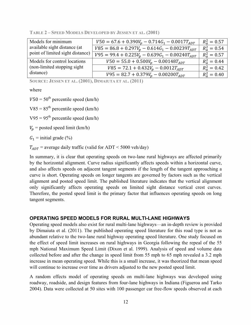
Polus et al. (2000) collected passenger car operating speed data on 162 tangent sections of two-lane rural highways in Minnesota, New York, Pennsylvania, Oregon, Washington, and Texas. Geometric design features at the data collection sites were used to develop 85th percentile operating speed models. The findings indicate that operating speeds on short horizontal tangents are controlled by the radius of the preceding and following curves. However, on long tangents, speed is controlled more by factors such as the posted speed limit and presence of enforcement than by geometric characteristics of the roadway (Polus, Fitzpatrick, and Fambro 2000). Jessen et al. (2001) collected free-flow speed data at crest vertical curves located on horizontal tangents in Nebraska. Individual vehicle operating speeds were measured on limited sight-distance crest curves in dry, daytime conditions using a magnetic vehicle counter and classifier. Comparison sites were also measured, using vertical curves with stopping sight distances that exceed minimum values. Linear regression was used to model the mean, 85th, and 95th percentile speeds. All three models were found to be a function of posted speed limit as well as initial grade and traffic volume. It is clear from Table 2 that grade only influences operating speeds on crest vertical curves if stopping sight distance is limited (Jessen et al. 2001). It is also notable that the influence of the posted speed limit is statistically significant in the models. This is discussed in further detail below.

12

TABLE 2 – SPEED MODELS DEVELOPED BY JESSEN ET AL. (2001)

Models for minimum available sight distance (at point of limited sight distance)

50 67.6 0.390 0.714 0.0017 0.57 85 86.8 0.297 0.614 0.00239 0.54 95 99.4 0.225 0.639 0.00240 0.57

Models for control locations (non-limited stopping sight distance)

50 55.0 0.500 0.00148 0.44 85 72.1 0.432 0.0012 0.42 95 82.7 0.379 0.00200 0.40

SOURCE: JESSEN ET AL. (2001), DIMAIUTA ET AL. (2011)

where

50 = 50th percentile speed (km/h)

V85 = 85th percentile speed (km/h)

V95 = 95th percentile speed (km/h)

= posted speed limit (km/h)

= initial grade (%)

= average daily traffic (valid for ADT < 5000 veh/day)

In summary, it is clear that operating speeds on two-lane rural highways are affected primarily by the horizontal alignment. Curve radius significantly affects speeds within a horizontal curve, and also affects speeds on adjacent tangent segments if the length of the tangent approaching a curve is short. Operating speeds on longer tangents are governed by factors such as the vertical alignment and posted speed limit. The published literature indicates that the vertical alignment only significantly affects operating speeds on limited sight distance vertical crest curves. Therefore, the posted speed limit is the primary factor that influences operating speeds on long tangent segments.

OPERATING SPEED MODELS FOR RURAL MULTI-LANE HIGHWAYS Operating speed models also exist for rural multi-lane highways—an in-depth review is provided by Dimaiuta et al. (2011). The published operating speed literature for this road type is not as abundant relative to the two-lane rural highway operating speed literature. One study focused on the effect of speed limit increases on rural highways in Georgia following the repeal of the 55 mph National Maximum Speed Limit (Dixon et al. 1999). Analysis of speed and volume data collected before and after the change in speed limit from 55 mph to 65 mph revealed a 3.2 mph increase in mean operating speed. While this is a small increase, it was theorized that mean speed will continue to increase over time as drivers adjusted to the new posted speed limit.

A random effects model of operating speeds on multi-lane highways was developed using roadway, roadside, and design features from four-lane highways in Indiana (Figueroa and Tarko 2004). Data were collected at 50 sites with 100 passenger car free-flow speeds observed at each

13

site. Free-flow conditions were identified as having at least a 5 second headway. Using OLS linear regression with panel data (PD) analysis, the following model was estimated:

54.027 4.764 4.492 6.509 1.652 0.00128

0.320 0.034 0.056 5.899 0.464 ∗ 0.464 ∗ 0.00048 ∗ 0.00422 ∗

0.477 ∗ (8)

where

= operating speeds

= 1 if the posted speed limit is 50 mph; 0 otherwise (55 mph baseline)



= 1 if the posted speed limit is 40 or 45 mph; 0 otherwise

= 1 if the road segment is in a rural area; 0 otherwise

= sight distance (ft)

= intersection density (# intersections/mile)

= external clear zone, distance from edge of traveled way to roadside object (ft)

= internal clear zone, distance from inside edge of traveled way to median barrier or opposing traffic lane (ft)

= standardize normal variable corresponding to a selected percentile speed

= total clear zone (ICLR + ECLR, ft)

= 1 of a two-way left-turn lane is present; 0 otherwise

This model indicates that operating speeds increase as posted speed limits increase. The 50 mph, 45 mph, and 40 mph speed limit indicators have coefficients of -4.76, -4.49, and -6.51 mph, respectively. This signifies that 45 and 50 mph posted speed limits are associated with operating speeds that are approximately 5 mph lower than roadway sections that have 55 mph posted speed limits (baseline). The 40 mph posted speed limit indicator suggests that operating speeds on these sections are only 6.51 mph lower than on sections with 55 mph posted speed limits. Another notable observation from the model is that clear zone width increases are associated with operating speed increases. Rural roadway segments are associated with operating speeds that are 1.7 mph higher than other areas. Finally, intersection density can significantly affect operating speeds—as the number of intersections within a segment increases, operating speeds decrease.

14

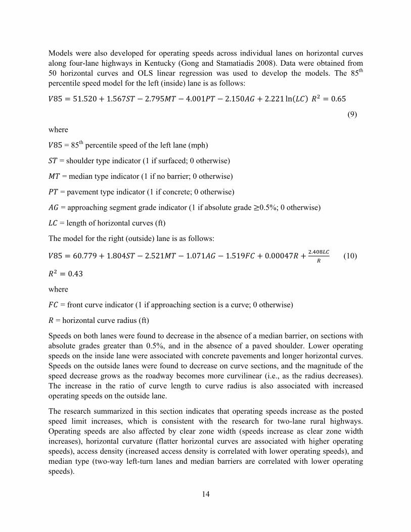
Models were also developed for operating speeds across individual lanes on horizontal curves along four-lane highways in Kentucky (Gong and Stamatiadis 2008). Data were obtained from 50 horizontal curves and OLS linear regression was used to develop the models. The 85th percentile speed model for the left (inside) lane is as follows:

85 51.520 1.567 2.795 4.001 2.150 2.221 ln 0.65

(9)

where

85 = 85th percentile speed of the left lane (mph)

= shoulder type indicator (1 if surfaced; 0 otherwise)

= median type indicator (1 if no barrier; 0 otherwise)

= pavement type indicator (1 if concrete; 0 otherwise)

= approaching segment grade indicator (1 if absolute grade 0.5%; 0 otherwise)

= length of horizontal curves (ft)

The model for the right (outside) lane is as follows:

85 60.779 1.804 2.521 1.071 1.519 0.00047 . (10)

0.43

where

= front curve indicator (1 if approaching section is a curve; 0 otherwise)

= horizontal curve radius (ft)

Speeds on both lanes were found to decrease in the absence of a median barrier, on sections with absolute grades greater than 0.5%, and in the absence of a paved shoulder. Lower operating speeds on the inside lane were associated with concrete pavements and longer horizontal curves. Speeds on the outside lanes were found to decrease on curve sections, and the magnitude of the speed decrease grows as the roadway becomes more curvilinear (i.e., as the radius decreases). The increase in the ratio of curve length to curve radius is also associated with increased operating speeds on the outside lane.

The research summarized in this section indicates that operating speeds increase as the posted speed limit increases, which is consistent with the research for two-lane rural highways. Operating speeds are also affected by clear zone width (speeds increase as clear zone width increases), horizontal curvature (flatter horizontal curves are associated with higher operating speeds), access density (increased access density is correlated with lower operating speeds), and median type (two-way left-turn lanes and median barriers are correlated with lower operating speeds).

15

ROLE OF POSTED SPEED LIMIT IN OPERATING SPEED MODELS Operating speed models that have included posted speed limit as an explanatory variable have found positive correlations between posted speed limit and operating speeds (Aljanahi, Rhodes, and Metcalfe 1999; Figueroa and Tarko 2004; Jessen et al. 2001; Polus, Fitzpatrick, and Fambro 2000). The relative lack of studies that include posted speed limit is due to the belief that significant correlation exists between the posted speed limit and other explanatory variables (such as horizontal curvature). This correlation occurs because the posted speed limit is related to the design speed, which affects the roadway alignment. However, omission of the posted speed limit from an operating speed model can result in omitted variable bias that is more damaging to a speed prediction model than the effects of serial correlation (Himes, Donnell, and Porter 2013). Himes, Donnell, and Porter (2013) also noted that the inclusion of the posted speed limit in an operating speed model only affects the efficiency of the explanatory variables but causes little to no bias in the coefficients. However, omission of the posted speed limit severely biases the coefficient estimates. This can lead to confusion for practitioners as they may overestimate their ability to control operating speeds with geometry and other roadway characteristics (Himes, Donnell, and Porter 2013).

STATE PRACTICES FOR SETTING POSTED SPEED LIMITS Very little information regarding speed limits set lower than engineering recommendation was found during an investigation of various state transportation agency speed limit policies. Closely related studies examined the opposite practice—raising posted speed limits (Kockelman et al, 2006), or increasing statewide maximum posted speed limits (Farmer 2016). The findings from these studies suggest that vehicle operating speeds increase in association with an increase in the posted speed limit, but do so by an amount less than the speed limit increase. Furthermore, increased speed limits are associated with a higher frequency of crashes and an increase in crash severity. However, opposite trends cannot necessarily be expected for posting speed limits lower than engineering recommendations.

Most states have statutory speed limits based on roadway classification, the presence of which implies that some roadways have posted speeds that are set lower than the designated design speed. However, states allow for changes to these speed limits based on site conditions, specifically based on operating speeds. The most common finding regarding the relationship between design speed and speed limit was the mention that design speed should be considered during an engineering study (Caltrans 2014; FDOT 2010; TXDOT 2012). Other state transportation agencies fail to make any mention of design speed, stressing that engineers consider the 85th percentile speed as well as the roadway environment when setting posted speed limits (Maryland Department of Transportation 2014; ODOT 2014; WSDOT 2014; State of Minnesota 2013). The most common finding that can be drawn from various state transportation agency practices is the emphasis on actual operating speeds of the roadway when setting posted speed limits. Perhaps this is not without merit, as the findings of NCHRP REPORT 504: DESIGN SPEED, OPERATING SPEED, AND POSTED SPEED PRACTICES found no noteworthy relationship

16

between design speed and either posted speed or operating speed, while a relationship between operating speed and posted speed limit was found to be statistically significant (Fitzpatrick et al. 2003). These operating speed models were developed using free flow speed data from 78 urban and suburban locations in Arkansas, Massachusetts, Missouri, Oregon, Tennessee, and Texas. In developing these models, vehicles were considered in a free-flow state if they had headways greater than five seconds and lags (headways of following vehicle) greater than three seconds. The following models for 85th percentile speed were estimated using linear regression:

85 7.675 0.98 0.90 (11)

85 16.089 0.831 0.054 0.92 (12)

where

85 = 85th percentile operating speed (mph)

= posted speed limit (mph)

= access density (pts/mile)

Fitzpatrick et al. (2003) also developed a model for rural multi-lane arterials. The model was estimated as follows:

85 36.453 0.517 0.81 (13)

A survey of state design speed practices was also part of NCHRP 504. Survey findings, representing 45 completed surveys from 40 states, indicated that most states used the functional classification or statutory speed limit as the basis for the design speed of a new roadway. Some states also considered predicted operating speeds when choosing a design speed.

Design Speed and Speed Limit Discord It is not uncommon for the posted speed limit to be set at levels that are not in harmony with the design speed of a roadway. A review of the literature on these scenarios can provide some insight into selecting speed limits lower than engineering recommendations. Three scenarios are discussed in which the posted speed limit is lower than the design speed of a roadway. Research investigating operating speeds and speed compliance under these scenarios is discussed in this section of the report. Speed limit transition zones are also described, as these represent scenarios in which the driver is aware that the roadway can be traveled at a higher speed but the posted speed limit is lower.

NATIONAL MAXIMUM SPEED LIMIT One well-known example of posted speed limits below design speeds is the implementation of the National Maximum Speed Limit (NMSL). In an effort to increase fuel efficiency and reduce

17

oil usage during the oil embargo of the 1970’s, the U.S. federal government enacted legislation that established a maximum speed limit of 55 mph on all Interstates (Friedman, Hedeker, and Richter 2009). This meant that many Interstates were constructed with geometric design features that had 70 mph design speeds. In many instances the posted speed limit on these roadways was higher than 55 mph before implementing the NMSL. Complying with the lower posted speed limit was likely difficult for drivers for several reasons. First, these drivers likely had prior experience traveling Interstates at higher speeds, and thus would have felt comfortable driving at these speeds. Second, Interstates were designed using uniform criteria that were the most “forgiving” (e.g., wider travel lanes, flatter horizontal curves) among criteria used for other roadway types. Due to this forgiving design, the inferred design speed of these facilities was likely much higher than 55 mph. This may confuse drivers as the roadway geometry provided no indication concerning compliance with the new posted speed limit of 55 mph.

Viewing speed limit compliance from a public policy standpoint, Meier and Morgan (1982) analyzed speed data from all 50 states to model the percent non-compliance based on environmental variables. Linear regression models were developed for two metrics: percent vehicles exceeding 55 mph (i.e., percent of non-compliance) and 85th percentile speed. Within a compliance theory framework, six variables were used to explain the speed variation of different states on NMSL facilities: miles driven per capita, size of the state (square miles), percent of Interstate highways, days of precipitation, altitude variation, and minimum driving age. The first three variables were found to be positively correlated in both models, while the last three were negatively correlated. Residuals for each state were used to discuss a true level of non-compliance. Instead of simply viewing a state’s 85th percentile operating speed and percent non-compliance on NMSL freeways, the authors suggest comparing the state’s metrics to those predicted by the models developed. States with highly positive residuals (i.e., those in which their actual speed metrics are much greater than those predicted) are those that had significant non-compliance issues with the NMSL. The data showed that Montana had a +3 percent residual for percent of vehicles exceeding a 55 mph speed limit and +0.93 mph residual for 85th percentile operating speed, suggesting non-compliance issues with respect to the NMSL (Meier and Morgan 1982). A similar national maximum speed limit existed in Israel (90 kilometers per hour or kph), and it was hypothesized that roughly half of the drivers exceeded the limit (Shinar 2007). The NMSL is likely the best example of posted speed limits that are lower than design and engineering recommended speeds.

WORK ZONE SPEED LIMITS Another common example of posted speed limits set lower than engineering recommendations occurs in work zones. Although work zone speed limits are temporary, vehicles often exceed them and travel at speeds near the permanent posted speed limit of the roadway. Research has shown that vehicles speeding prior to entering a work zone still travel at high speeds and violate the temporary speed limit, although they do reduce their speeds (Benekohal and Wang 1994).

In an attempt to understand speed limit compliance in work zones, tobit models were developed to model speed limit compliance at three separate, characteristically different work zones in

18

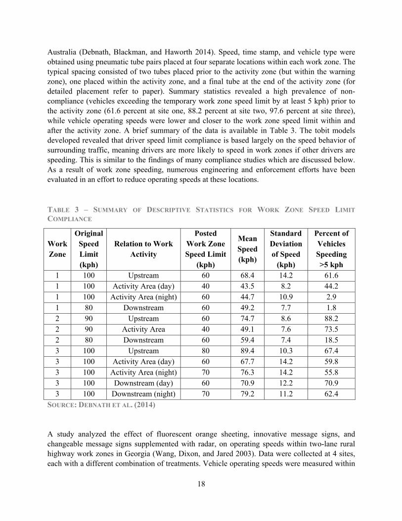
Australia (Debnath, Blackman, and Haworth 2014). Speed, time stamp, and vehicle type were obtained using pneumatic tube pairs placed at four separate locations within each work zone. The typical spacing consisted of two tubes placed prior to the activity zone (but within the warning zone), one placed within the activity zone, and a final tube at the end of the activity zone (for detailed placement refer to paper). Summary statistics revealed a high prevalence of non-compliance (vehicles exceeding the temporary work zone speed limit by at least 5 kph) prior to the activity zone (61.6 percent at site one, 88.2 percent at site two, 97.6 percent at site three), while vehicle operating speeds were lower and closer to the work zone speed limit within and after the activity zone. A brief summary of the data is available in Table 3. The tobit models developed revealed that driver speed limit compliance is based largely on the speed behavior of surrounding traffic, meaning drivers are more likely to speed in work zones if other drivers are speeding. This is similar to the findings of many compliance studies which are discussed below. As a result of work zone speeding, numerous engineering and enforcement efforts have been evaluated in an effort to reduce operating speeds at these locations.

TABLE 3 – SUMMARY OF DESCRIPTIVE STATISTICS FOR WORK ZONE SPEED LIMIT COMPLIANCE

Work Zone

Original Speed Limit (kph)

Relation to Work Activity

Posted Work Zone Speed Limit

(kph)

Mean Speed (kph)

Standard Deviation of Speed

(kph)

Percent of Vehicles Speeding >5 kph

1 100 Upstream 60 68.4 14.2 61.6 1 100 Activity Area (day) 40 43.5 8.2 44.2 1 100 Activity Area (night) 60 44.7 10.9 2.9 1 80 Downstream 60 49.2 7.7 1.8 2 90 Upstream 60 74.7 8.6 88.2 2 90 Activity Area 40 49.1 7.6 73.5 2 80 Downstream 60 59.4 7.4 18.5 3 100 Upstream 80 89.4 10.3 67.4 3 100 Activity Area (day) 60 67.7 14.2 59.8 3 100 Activity Area (night) 70 76.3 14.2 55.8 3 100 Downstream (day) 60 70.9 12.2 70.9 3 100 Downstream (night) 70 79.2 11.2 62.4

SOURCE: DEBNATH ET AL. (2014)

A study analyzed the effect of fluorescent orange sheeting, innovative message signs, and changeable message signs supplemented with radar, on operating speeds within two-lane rural highway work zones in Georgia (Wang, Dixon, and Jared 2003). Data were collected at 4 sites, each with a different combination of treatments. Vehicle operating speeds were measured within

19

the work zone and upstream of the work zone. Analysis of the data revealed small speed reductions (less than 3 mph) when fluorescent orange sheeting and innovative message signs were used. The novelty effect (i.e., adjustment of behavior based on the introduction of a new treatment) reduced the impact of the sheeting at some sites, while the innovative message signs failed to maintain any speed reduction. The biggest speed reduction was associated with changeable message signs with radar (CMSRs), which resulted in operating speed reductions up to 8 mph. A novelty effect was not found when using CMSRs in work zones. It should be noted that no information concerning the difference between the work zone speed limit and upstream speed limit , meaning there is no context for viewing these speed reductions in terms of a change in the regulatory speed limit. It is clear from this study that speed compliance with signage is challenging, yet possible. General guidelines for the design of work zones, including discussion on speed enforcement, are discussed in NCHRP REPORT 581 (Mahoney et al. 2007).

SEASONAL SPEED LIMITS Another scenario that considers the impacts of speed limit reductions on vehicle operating speeds is the use of seasonal speed limits. Separate studies have investigated the effect of seasonal posted speed limit reductions in Finland. Finland has consistently experimented with lower winter speed limits from November to February with the goal of reducing crashes related to poor roadway conditions during the winter. Peltola (2000) found that a reduction of the speed limit from 100 km/h to 80 km/h using static speed limit signs reduced mean operating speeds of all vehicles by 3.8 km/h (compared to a 3.3 km/h reduction on control roads with no changed speed limit). Passenger car operating speeds were reduced by more than 5 km/h. Also, the variation in individual speeds was reduced, primarily at sites with higher posted speed limits. Data were obtained by measuring point speeds with radar at a set of locations per month for a two-year data collection period that began one month prior to the first speed limit reduction. Data collection resulted in 140,000 individual vehicle speed measurements. This study was performed using an observational before-after design with comparison sites with 100 treatment and 147 control sites (Peltola 2000).

Similarly, Rämä (2001) found a mean speed reduction of 3.4 km/h for a seasonal speed limit reduction of 120 km/h to 100 km/h using variable message speed limit signs, along with a reduction of speed variance. Speed data for this study were obtained using loop sensors. While both of these reductions were found to be statistically significant, the practical significance is nominal, considering the posted speed limit reduction was 20 km/h.

The studies discussed above reveal issues with speed limit compliance. It is clear that when faced with a speed limit reduction, drivers tend to disregard the lower posted speed limit. This is likely due to drivers feeling that the reduced posted speed is not rational when considering the surrounding roadway environment. One factor these studies did not consider is enforcement. The effect of enforcement is discussed in a subsequent section, as well as how a driver chooses an operating speed and how speed limit compliance plays into this decision.

20

SPEED LIMIT TRANSITION ZONES Speed transition zones are common on rural two-lane highways. These zones occur when a high-speed facility traverses through a town or area with many conflicts for which the original speed limit is no longer appropriate. NCHRP REPORT 737 provides design guidelines for agencies implementing high-to-low speed transition zones (Torbic et al. 2012). Research has demonstrated the factors that affect operating speed changes in transition zones (Cruzado and Donnell 2009; Cruzado and Donnell 2010). Cruzado and Donnell (2009) studied the effectiveness of dynamic speed display signs on free-flow operating speeds on two-lane rural highway transition zones in Pennsylvania. These signs consist of a speed limit sign and a dynamic message sign. The dynamic message sign reports the speed measured by the radar device to the driver of the oncoming vehicle, providing drivers with real-time feedback regarding their compliance. Data were collected before implementation, during implementation, and after the signs were removed. Analysis of the data revealed that dynamic speed display signs reduced operating speeds by about 6 mph during implementation, but this reduction diminished upon removal of the devices.

Cruzado and Donnell (2010) examined how various site characteristics affected speed reduction in transition zones on two-lane rural highways in Pennsylvania. Twenty potential sites were identified based on the following criteria:

1. Presence of a Reduced Speed Ahead (W3-5) sign 2. No major signalized or stop-controlled intersections 3. Low percentage of heavy vehicles (less than 10 percent) 4. Low traffic volumes (to maximize free-flow observations) 5. Smooth pavement surface with good pavement markings

At each site, at least 100 free-flow vehicle observations were obtained from the following three locations: 500 feet prior to the Reduced Speed Ahead sign, at the Reduced Speed Ahead Sign, and at the lowered posted speed limit sign. Linear and multilevel regression models were used to predict speed reduction in the transition zone. These findings indicate that all factors considered (except the presence of a curve ahead warning sign) increase the speed reduction in the transition zone. This suggests that numerous countermeasures can be implemented to reduce speeds in transition zones and improve compliance with the lowered posted speed limit, including: introducing a curb, installing an intersection ahead warning sign, installing a curve ahead warning sign and using a longer transition zone.

SPEED LIMIT COMPLIANCE AND ENFORCEMENT Extensive research has been performed by both psychologists and engineers attempting to understand driver speed choice and the likelihood of compliance with the posted speed limit. There have also been numerous studies investigating how enforcement determines driver speed choice, compliance, and operating speeds.

21

SPEED CHOICE AND COMPLIANCE When selecting a speed on a given roadway segment, a driver considers many factors. These include roadway characteristics (i.e., width, speed curvature), vehicle characteristics (i.e., power, comfort), surrounding traffic (i.e., average speed, percentage of heavy vehicles), and the environment (i.e., weather, lighting, speed limit) (WHO 2004). Upon inclusion of internal factors (i.e., age, risk acceptance, driving history), both consciously and subconsciously, a driver then selects a desired speed. While all of these factors play into speed choice, they affect the decision at different magnitudes. A survey conducted by the Transport Research Laboratory found that site characteristics had the biggest impact on driver speed choice (Quimby et al. 1999). This is evidenced by the relationship between operating speeds and geometric characteristics previously shown in the operating speed models. Other research has found that driver speed choice, especially in relation to a willingness to exceed the posted speed limit, is based largely on the speed of other vehicles (Haglund and Aberg 2000; C. Wang, Dixon, and Jared 2003). It has also been shown that drivers who have experience violating the speed limit are more likely to continue this behavior in the future as a result of developing a speeding habit (Elliott, Armitage, and Baughan 2003; De Pelsmacker and Janssens 2007). A more detailed discussion of this topic can be found in TRAFFIC SAFETY AND HUMAN BEHAVIOR (D. Shinar 2007).

ENFORCEMENT Speed enforcement is one of the few ways to ensure compliance with a posted speed limit. Most speed enforcement is performed by police officers, but some agencies utilize tools such as speed cameras.

Washington, D.C., implemented speed cameras mounted on police cruisers (Retting and Farmer 2003). These cameras use Doppler radar to monitor vehicle speeds and a violation of the speed limit triggered the camera to take a picture of the vehicle exceeding the regulatory speed. Sixty enforcement sites were identified, and from August 1 to October 1, speed cameras were deployed twice per week. Implementation of this program was preceded by a public awareness campaign and the enforcement sites were signed to warn drivers of the use of speed cameras. Seven of the 60 sites were randomly selected for the study, with eight similar comparison sites selected in Baltimore, Maryland. Speed data were collected using the speed camera equipment utilized by the police both before and after implementation. Analysis of the data revealed a statistically significant reduction in average speed of 14 percent and a reduction in non-compliance, compared to no reduction on the comparison sites.

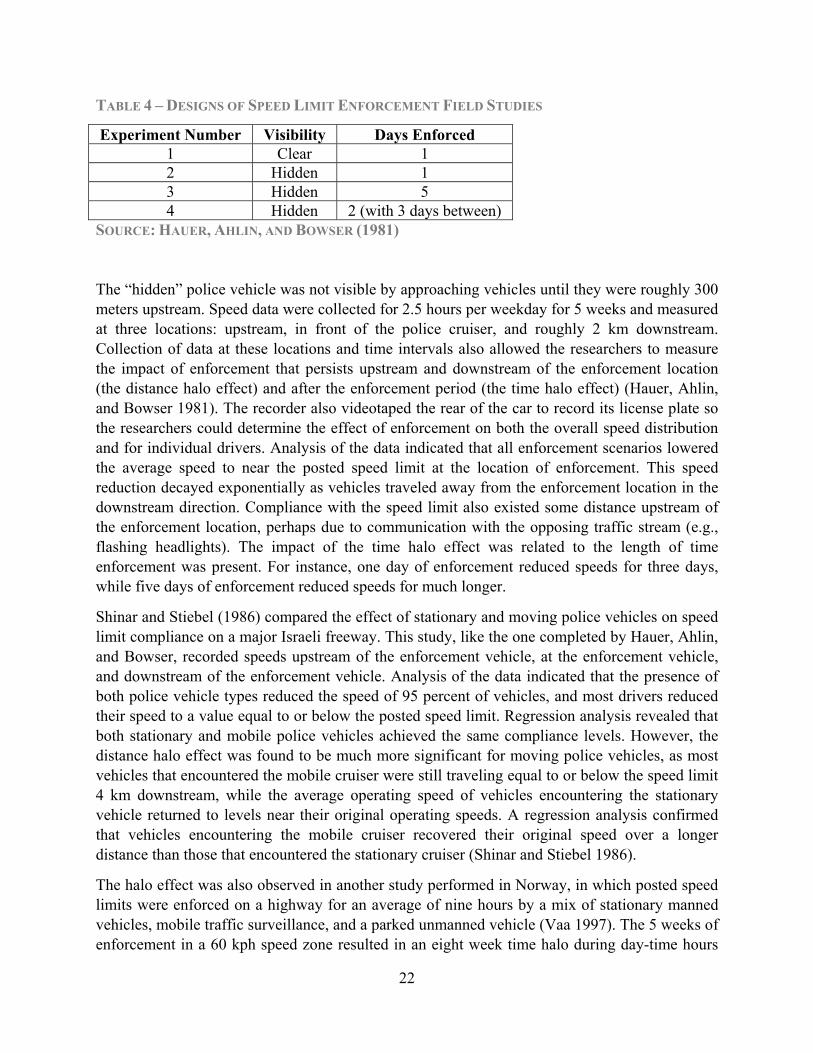
A study of semi-rural highways in Canada by Hauer, Ahlin, and Bowser (1981) examined four enforcement scenarios using a single police car with radar in four separate field studies. Details of the four scenarios are shown in Table 4.

22

TABLE 4 – DESIGNS OF SPEED LIMIT ENFORCEMENT FIELD STUDIES

Experiment Number Visibility Days Enforced 1 Clear 1 2 Hidden 1 3 Hidden 5 4 Hidden 2 (with 3 days between)

SOURCE: HAUER, AHLIN, AND BOWSER (1981)

The “hidden” police vehicle was not visible by approaching vehicles until they were roughly 300 meters upstream. Speed data were collected for 2.5 hours per weekday for 5 weeks and measured at three locations: upstream, in front of the police cruiser, and roughly 2 km downstream. Collection of data at these locations and time intervals also allowed the researchers to measure the impact of enforcement that persists upstream and downstream of the enforcement location (the distance halo effect) and after the enforcement period (the time halo effect) (Hauer, Ahlin, and Bowser 1981). The recorder also videotaped the rear of the car to record its license plate so the researchers could determine the effect of enforcement on both the overall speed distribution and for individual drivers. Analysis of the data indicated that all enforcement scenarios lowered the average speed to near the posted speed limit at the location of enforcement. This speed reduction decayed exponentially as vehicles traveled away from the enforcement location in the downstream direction. Compliance with the speed limit also existed some distance upstream of the enforcement location, perhaps due to communication with the opposing traffic stream (e.g., flashing headlights). The impact of the time halo effect was related to the length of time enforcement was present. For instance, one day of enforcement reduced speeds for three days, while five days of enforcement reduced speeds for much longer.

Shinar and Stiebel (1986) compared the effect of stationary and moving police vehicles on speed limit compliance on a major Israeli freeway. This study, like the one completed by Hauer, Ahlin, and Bowser, recorded speeds upstream of the enforcement vehicle, at the enforcement vehicle, and downstream of the enforcement vehicle. Analysis of the data indicated that the presence of both police vehicle types reduced the speed of 95 percent of vehicles, and most drivers reduced their speed to a value equal to or below the posted speed limit. Regression analysis revealed that both stationary and mobile police vehicles achieved the same compliance levels. However, the distance halo effect was found to be much more significant for moving police vehicles, as most vehicles that encountered the mobile cruiser were still traveling equal to or below the speed limit 4 km downstream, while the average operating speed of vehicles encountering the stationary vehicle returned to levels near their original operating speeds. A regression analysis confirmed that vehicles encountering the mobile cruiser recovered their original speed over a longer distance than those that encountered the stationary cruiser (Shinar and Stiebel 1986).

The halo effect was also observed in another study performed in Norway, in which posted speed limits were enforced on a highway for an average of nine hours by a mix of stationary manned vehicles, mobile traffic surveillance, and a parked unmanned vehicle (Vaa 1997). The 5 weeks of enforcement in a 60 kph speed zone resulted in an eight week time halo during day-time hours

23

(9am-3pm) while the 80 kph speed zone experienced a six week time halo during all hours except 6am-3pm. This study also found a statistically significant reduction in speeding vehicles, indicating a reduction in speed variance.

An observational before-after study of speed and safety on a 22 km long corridor of freeway in British Columbia was performed to estimate the effect of 12 stationary speed cameras (Chen, Meckle, and Wilson 2002). These speed cameras operated from 6 am to 11 pm and were programmed to photograph offenders violating the posted speed limit by greater than 11 kph. After collecting speed data from millions of vehicles using both the speed cameras and induction loops, it was found that mean speeds at individual speed camera locations dropped to or below the posted speed limit, while a speed reduction of more than 2 kph was found along the entire corridor. This indicates that these individual cameras have a significant distance halo. Researchers also found a statistically significant reduction of speed variance on the corridor of 0.5 (kph)2. Since enforcement was not removed, it was not possible to evaluate the existence of a time halo effect. However, the researchers noted that the drop in speed was consistent over the two year study period. An Empirical Bayes before-after study was also performed to determine the safety effect of the enforcement system. The results of this analysis found an expected crash reduction of 16 percent (standard deviation of 7 percent) over the entire corridor. A summary of the halo effects is shown in Table 5. Overall, it is clear that speed limit enforcement can reduce vehicle operating speeds to levels consistent with posted the speed limit. However, the distance and time halo effects indicate that the speed reduction is not permanent unless the enforcement is permanent (e.g., as would occur with speed cameras).

24

TABLE 5 – SUMMARY OF HALO EFFECTS

Study Enforcement Type

Enforcement Duration

Distance Halo,

Upstream

Distance Halo,

Downstream Time Halo

Hauer, Ahlin, Bowser (1981)

Visible Police Cruiser 1 day

Reduction reported, but no quantity

given

Effect reduced by half every 900 meters

from enforcement

n/a


Hidden Police Cruiser 1 day


given


from enforcement

2 days


Hidden Police Cruiser 5 days (M-F)


given


from enforcement

6 days


Hidden Police Cruiser

2 days (with three days separating)


given


from enforcement

3 days

Shinar and Stiebel (1986)

Stationary Police Cruiser 1 day Not

Measured SR=-

3.4+0.6*SE1 Not

Measured Shinar and

Stiebel (1986) Mobile Police

Cruiser 1 day Not Measured

SR=-6.7+0.3*SE

Not Measured

Vaa (1997) (80 kph speed

zones)

Mixed Cruisers 6 weeks Not

Measured Not Measured 8 weeks

(from 9 am-3 pm)

Vaa (1997) (60 kph speed

zones)

Mixed Cruisers 6 weeks Not

Measured Not Measured 6 weeks (all hours but 6 am – 3 pm)

Chen, Meckle, Wilson (2002)

Mounted Speed

Cameras

2 years (entire study

period)

Speeds reduced over entire corridor, not just camera

locations

Not Measured

SR = Speed Resumption (recovery of initial as speed), SE = Speed Excess (speed limit excess measured upstream of enforcement)

THE HANDBOOK OF ROAD SAFETY MEASURES (Rune Elvik et al. 2009) contains a full chapter (Part II, Chapter 8) on the effects of police enforcement and sanctions. The chapter indicates that

25

enforcement is effective in reducing operating speeds as well as improving safety. Benefit-cost (B/C) ratios are supplied for numerous enforcement practices. Two notable B/C ratios are tripling stationary speed enforcement (B/C = 1.5) and automatic speed enforcement (B/C ranges from 2 to 27). These indicate that typical enforcement strategies do see a return on investment, mainly from safety benefits.

SPEED AND SAFETY As mentioned earlier, it has long been hypothesized that increases in speeds should be correlated with increases in both crash frequency and crash severity. However, there seems to be a lack of empirical evidence on the relationship between speed and safety, exemplified by the fact that there are no crash modification factors (CMFs) included in AASHTO’s HIGHWAY SAFETY MANUAL related to speed (AASHTO 2010). This is due to a lack of consistent empirical findings in regards to the relationship between speed and crash frequency. The oft cited Solomon curve (Solomon 1964), a U-shaped curve depicting a unimodal, convex relationship between speed and crash frequency, suggests that crash frequencies are minimized at about 60 mph (see Figure 2). However, this curve cannot be trusted due to a failure to remove slow-moving turning vehicles from the database, which unfairly increases crash frequencies at the low-end of the speed curve (Hauer 2009). Based on these data, Solomon (1964) also concluded that speed variance is a predictor of the probability of a crash occurring, proposing that as a vehicle’s speed deviates from the mean speed on a roadway, the probability of the vehicle being involved in a crash increases exponentially. However, this conclusion suffers from the same errors mentioned earlier (failure to remove turning vehicles from the data set).

FIGURE 2 – CRASH INVOLVEMENT AS A FUNCTION OF SPEED FOR DAYTIME AND NIGHTTIME CRASHES

SOURCE: SOLOMON (1964)

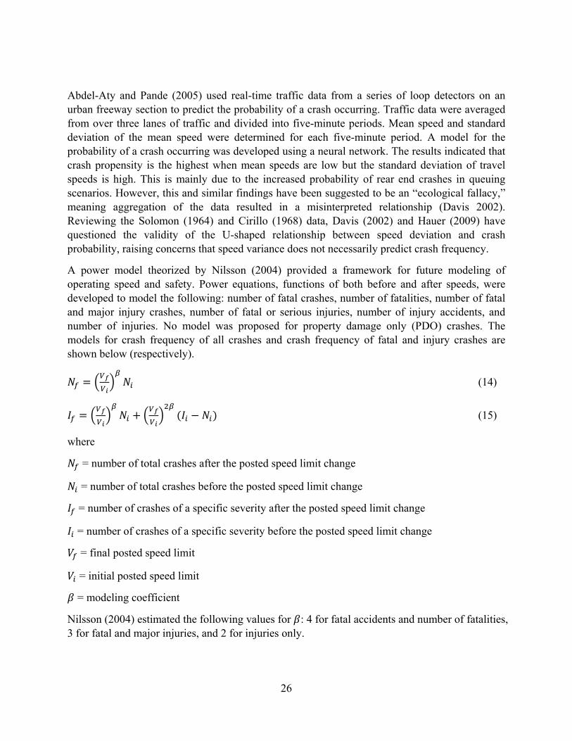
26

Abdel-Aty and Pande (2005) used real-time traffic data from a series of loop detectors on an urban freeway section to predict the probability of a crash occurring. Traffic data were averaged from over three lanes of traffic and divided into five-minute periods. Mean speed and standard deviation of the mean speed were determined for each five-minute period. A model for the probability of a crash occurring was developed using a neural network. The results indicated that crash propensity is the highest when mean speeds are low but the standard deviation of travel speeds is high. This is mainly due to the increased probability of rear end crashes in queuing scenarios. However, this and similar findings have been suggested to be an “ecological fallacy,” meaning aggregation of the data resulted in a misinterpreted relationship (Davis 2002). Reviewing the Solomon (1964) and Cirillo (1968) data, Davis (2002) and Hauer (2009) have questioned the validity of the U-shaped relationship between speed deviation and crash probability, raising concerns that speed variance does not necessarily predict crash frequency.

A power model theorized by Nilsson (2004) provided a framework for future modeling of operating speed and safety. Power equations, functions of both before and after speeds, were developed to model the following: number of fatal crashes, number of fatalities, number of fatal and major injury crashes, number of fatal or serious injuries, number of injury accidents, and number of injuries. No model was proposed for property damage only (PDO) crashes. The models for crash frequency of all crashes and crash frequency of fatal and injury crashes are shown below (respectively).

(14)

(15)

where

= number of total crashes after the posted speed limit change

= number of total crashes before the posted speed limit change

= number of crashes of a specific severity after the posted speed limit change

= number of crashes of a specific severity before the posted speed limit change

= final posted speed limit

= initial posted speed limit

= modeling coefficient

Nilsson (2004) estimated the following values for : 4 for fatal accidents and number of fatalities, 3 for fatal and major injuries, and 2 for injuries only.

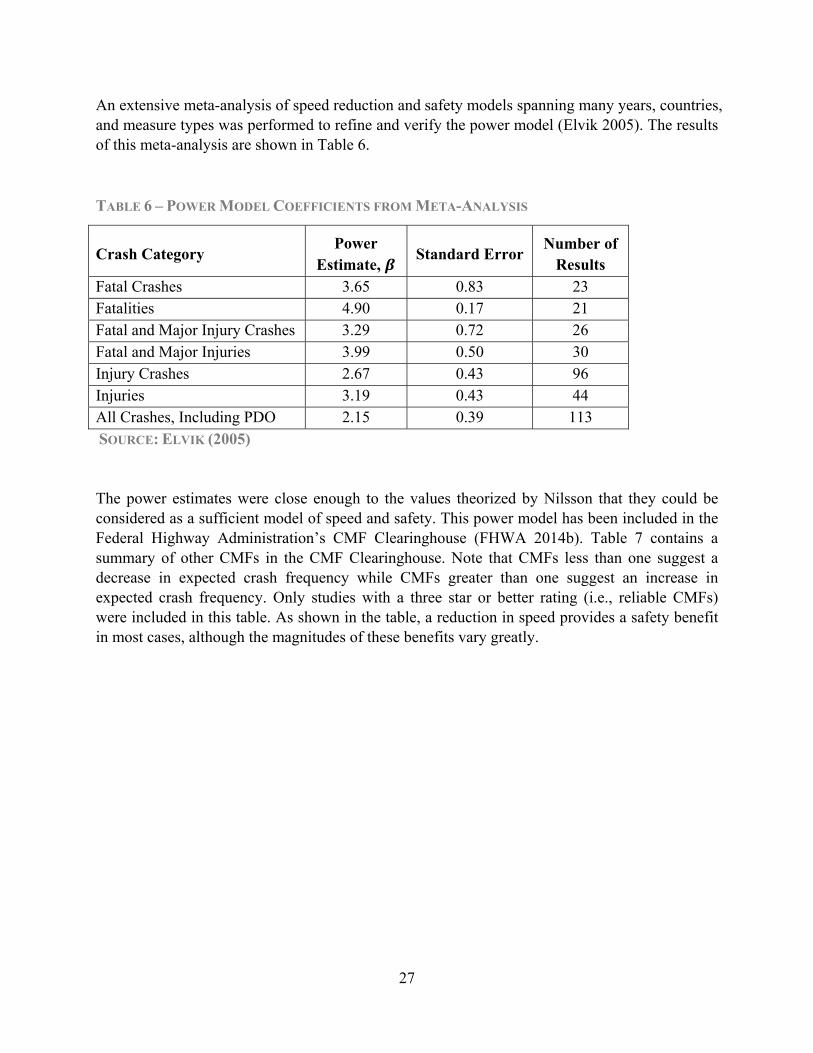
27

An extensive meta-analysis of speed reduction and safety models spanning many years, countries, and measure types was performed to refine and verify the power model (Elvik 2005). The results of this meta-analysis are shown in Table 6.

TABLE 6 – POWER MODEL COEFFICIENTS FROM META-ANALYSIS

Crash Category Power

Estimate, Standard Error Number of

Results Fatal Crashes 3.65 0.83 23 Fatalities 4.90 0.17 21 Fatal and Major Injury Crashes 3.29 0.72 26 Fatal and Major Injuries 3.99 0.50 30 Injury Crashes 2.67 0.43 96 Injuries 3.19 0.43 44 All Crashes, Including PDO 2.15 0.39 113 SOURCE: ELVIK (2005)

The power estimates were close enough to the values theorized by Nilsson that they could be considered as a sufficient model of speed and safety. This power model has been included in the Federal Highway Administration’s CMF Clearinghouse (FHWA 2014b). Table 7 contains a summary of other CMFs in the CMF Clearinghouse. Note that CMFs less than one suggest a decrease in expected crash frequency while CMFs greater than one suggest an increase in expected crash frequency. Only studies with a three star or better rating (i.e., reliable CMFs) were included in this table. As shown in the table, a reduction in speed provides a safety benefit in most cases, although the magnitudes of these benefits vary greatly.

28

TABLE 7 – SUMMARY OF SPEED RELATED CMF STUDIES (FHWA 2014B)

Study Treatment Quality

(5 is highest)

CMF Crash Type Severity Area

Elvik, Christensen, and Amundsen (2004)

10% reduction, mean speed

5 0.85 All Injury All 4 0.68 All Fatal All 3 0.9 All PDO All


4 0.56 All Fatal All 4 0.78 All Injury All 3 0.85 All PDO All

5% increase, mean speed




Ksaibati and Evans (2009)

Change 85th percentile speed from x to y

3 e^0.0111(y-x) All Rural

H. Chen et al. (2011) Change freeway speed Limit from x to y mph

3 e^-0.017(y-x) All Fatal and

Major Injury

N/A

Acqua and Russo (2011)

Change mean speed (kph) 3 e^0.24556(y-x) All Fatal and

Injury Rural

Park, Park, and Lomax (2010)

Decrease posted speed limit on expressways

4 0.8553 All All N/A

4 0.9123 Speed Related All N/A

4 1.0358 All Fatal and

Major Injury

N/A

4 0.7915 All Minor Injury N/A

Wei and Tarko (2011) Increase speed

limit from x to y (mph)

3 100(1-e^0.158(y-x)) Rear End All Urban and

Suburban

Z. Wang et al. (2011) 3 e^(-0.0136(y-x)) Truck Related All N/A

Dixon, Abdel-Rahim, and Elbassuoni (2012)

Install 10 mph differential speed limit on rural interstate highways

3 0.914 All,

Truck Related

All Rural

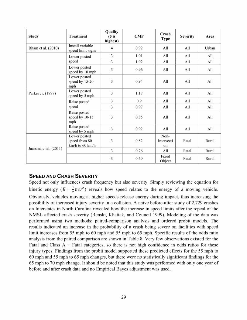
29

Study Treatment Quality

(5 is highest)

CMF Crash Type Severity Area

Bham et al. (2010) Install variable speed limit signs 4 0.92 All All Urban

Parker Jr. (1997)

Lower posted speed

3 1.01 All All All 3 1.02 All All All

Lower posted speed by 10 mph 3 0.96 All All All

Lower posted speed by 15-20 mph

3 0.94 All All All

Lower posted speed by 5 mph 3 1.17 All All All

Raise posted speed

3 0.9 All All All 3 0.97 All All All

Raise posted speed by 10-15 mph

3 0.85 All All All

Raise posted speed by 5 mph 3 0.92 All All All

Jaarsma et al. (2011)

Lower posted speed from 80 km/h to 60 km/h

3 0.82 Non-

Intersection

Fatal Rural

3 0.76 All Fatal Rural

3 0.69 Fixed Object Fatal Rural

SPEED AND CRASH SEVERITY Speed not only influences crash frequency but also severity. Simply reviewing the equation for kinetic energy ( ) reveals how speed relates to the energy of a moving vehicle. Obviously, vehicles moving at higher speeds release energy during impact, thus increasing the possibility of increased injury severity in a collision. A naïve before-after study of 2,729 crashes on Interstates in North Carolina revealed how the increase in speed limits after the repeal of the NMSL affected crash severity (Renski, Khattak, and Council 1999). Modeling of the data was performed using two methods: paired-comparison analysis and ordered probit models. The results indicated an increase in the probability of a crash being severe on facilities with speed limit increases from 55 mph to 60 mph and 55 mph to 65 mph. Specific results of the odds ratio analysis from the paired comparison are shown in Table 8. Very few observations existed for the Fatal and Class A + Fatal categories, so there is not high confidence in odds ratios for these injury types. Findings from the probit model supported these predicted effects for the 55 mph to 60 mph and 55 mph to 65 mph changes, but there were no statistically significant findings for the 65 mph to 70 mph change. It should be noted that this study was performed with only one year of before and after crash data and no Empirical Bayes adjustment was used.

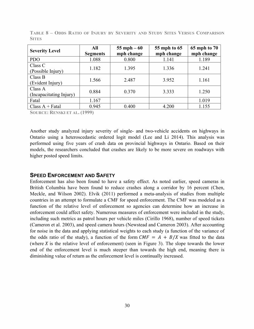
30

TABLE 8 – ODDS RATIO OF INJURY BY SEVERITY AND STUDY SITES VERSUS COMPARISON SITES

Severity Level All Segments

55 mph – 60 mph change

55 mph to 65 mph change

65 mph to 70 mph change

PDO 1.088 0.800 1.141 1.189 Class C (Possible Injury) 1.182 1.395 1.336 1.241

Class B (Evident Injury) 1.566 2.487 3.952 1.161

Class A (Incapacitating Injury) 0.884 0.370 3.333 1.250

Fatal 1.167 1.019 Class A + Fatal 0.945 0.400 4.200 1.155 SOURCE: RENSKI ET AL. (1999)

Another study analyzed injury severity of single- and two-vehicle accidents on highways in Ontario using a heteroscedastic ordered logit model (Lee and Li 2014). This analysis was performed using five years of crash data on provincial highways in Ontario. Based on their models, the researchers concluded that crashes are likely to be more severe on roadways with higher posted speed limits.

SPEED ENFORCEMENT AND SAFETY Enforcement has also been found to have a safety effect. As noted earlier, speed cameras in British Columbia have been found to reduce crashes along a corridor by 16 percent (Chen, Meckle, and Wilson 2002). Elvik (2011) performed a meta-analysis of studies from multiple countries in an attempt to formulate a CMF for speed enforcement. The CMF was modeled as a function of the relative level of enforcement so agencies can determine how an increase in enforcement could affect safety. Numerous measures of enforcement were included in the study, including such metrics as patrol hours per vehicle miles (Cirillo 1968), number of speed tickets (Cameron et al. 2003), and speed camera hours (Newstead and Cameron 2003). After accounting for noise in the data and applying statistical weights to each study (a function of the variance of the odds ratio of the study), a function of the form / was fitted to the data (where is the relative level of enforcement) (seen in Figure 3). The slope towards the lower end of the enforcement level is much steeper than towards the high end, meaning there is diminishing value of return as the enforcement level is continually increased.

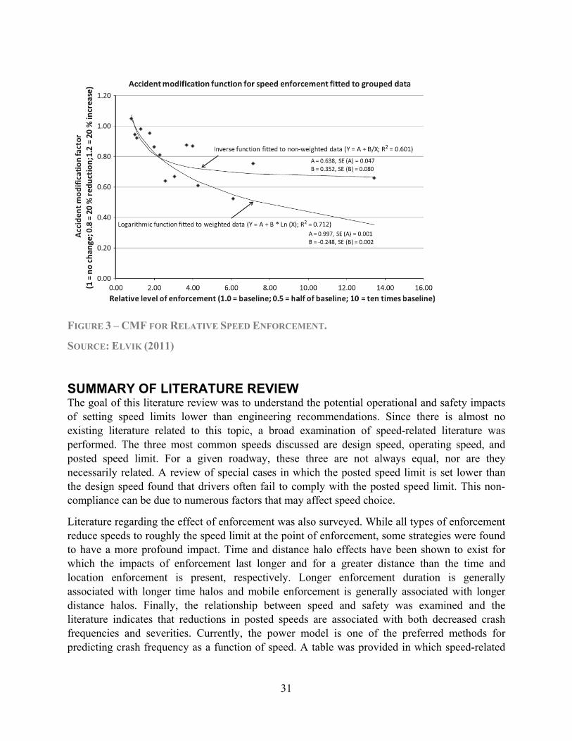
31

FIGURE 3 – CMF FOR RELATIVE SPEED ENFORCEMENT.

SOURCE: ELVIK (2011)

SUMMARY OF LITERATURE REVIEW The goal of this literature review was to understand the potential operational and safety impacts of setting speed limits lower than engineering recommendations. Since there is almost no existing literature related to this topic, a broad examination of speed-related literature was performed. The three most common speeds discussed are design speed, operating speed, and posted speed limit. For a given roadway, these three are not always equal, nor are they necessarily related. A review of special cases in which the posted speed limit is set lower than the design speed found that drivers often fail to comply with the posted speed limit. This non-compliance can be due to numerous factors that may affect speed choice.

Literature regarding the effect of enforcement was also surveyed. While all types of enforcement reduce speeds to roughly the speed limit at the point of enforcement, some strategies were found to have a more profound impact. Time and distance halo effects have been shown to exist for which the impacts of enforcement last longer and for a greater distance than the time and location enforcement is present, respectively. Longer enforcement duration is generally associated with longer time halos and mobile enforcement is generally associated with longer distance halos. Finally, the relationship between speed and safety was examined and the literature indicates that reductions in posted speeds are associated with both decreased crash frequencies and severities. Currently, the power model is one of the preferred methods for predicting crash frequency as a function of speed. A table was provided in which speed-related

32

crash modification factors from the CMF Clearinghouse were explained. Finally, the safety benefits of enforcement were covered.

The findings of this literature review informed the data collection plan, which is described in a subsequent section of this report. Free-flow operating speed studies seem to be the main tool for assessing operating speeds on a facility. Speeds in these studies can be measured using various methods including radar, pneumatic road tubes, and on-pavement sensors. Previous studies indicate that a vehicle is in “free-flow” conditions if its lead headway is at least five seconds and a trail headway of three seconds. The operating speed models discussed in this section of the report indicate that posted speed limits, design speed, and geometric design features are associated with operating speeds. Therefore, the treatment sites in the present study (locations with speed limits set lower than engineering recommendations) should be similar to reference group sites with regards to geometric features and engineering-recommended speed limits.

33

SURVEY OF AGENCY PRACTICES This section documents the results of a survey administered to representatives from each state transportation agency on current practices with respect to setting speed limits lower than engineering recommendation. The goal of the survey was to determine if other state transportation agencies have experience setting posted speed limits lower than engineering recommendations and, if so, to identify any guidance that might exist for this practice. The survey was hosted through Penn State and Qualtrics, an online survey software (Qualtrics 2014). Figure 4 depicts the structure of the survey as a flowchart. Each respondent was asked which state agency he or she represents and if his or her state agency sets posted speed limits lower than engineering recommendations. If the response to this question was yes, the respondent was asked if the representative’s state has evaluated the impacts of this practice; if the agency has any documentation that may be helpful for the analysis; if the state has guidelines to determine the level of enforcement required to achieve a desired level of compliance on these roadways; and if there were any issues related to this practice. If the respondent indicated that his or her agency did not practice setting speed limits lower than engineering recommendations, the respondent was asked if there were any conditions that the agency would consider such a practice; if the agency had experience quantifying speed limit compliance in the presence of enforcement; and, requested any documentation on speed limit compliance and enforcement. Documentation could either be uploaded through the survey platform or emailed directly to the research team. The full, text-based version of the survey can be found in Appendix A.

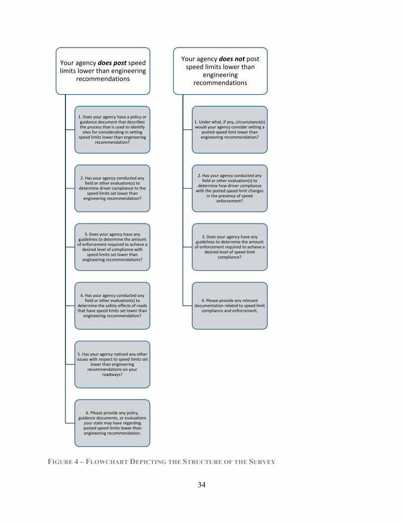
34

FIGURE 4 – FLOWCHART DEPICTING THE STRUCTURE OF THE SURVEY

Your agency does post speed limits lower than engineering

recommendations

1. Does your agency have a policy or guidance document that describes the process that is used to identify sites for considerating in setting

speed limits lower than engineering recommendation?

2. Has your agency conducted any field or other evaluation(s) to

determine driver compliance to the speed limits set lower than

engineering recommendation?

3. Does your agency have any guidelines to determine the amount of enforcement required to achieve a

desired level of compliance with speed limits set lower than

engineering recommendations?


determine the safety effects of roads that have speed limits set lower than

engineering recommendation?

5. Has your agency noticed any other issues with respect to speed limits set

lower than engineering recommendations on your

roadways?

6. Please provide any policy, guidance documents, or evaluations

your state may have regarding posted speed limits lower than engineering recommendation.

Your agency does not post speed limits lower than

engineering recommendations

1. Under what, if any, circumstance(s) would your agency consider setting a

posted speed limit lower than engineering recommendation?


determine how driver compliance with the posted speed limit changes

in the presence of speed enforcement?

3. Does your agency have any guidelines to determine the amount of enforcement required to achieve a

desired level of speed limit compliance?

4. Please provide any relevant documentation related to speed limit

compliance and enforcement.

35

State agency representatives selected as potential survey respondents were obtained through the AASHTO Subcommittee on Traffic Engineering (AASTHO 2014). All members that represented a state agency (including the District of Columbia and Puerto Rico, and excluding Montana) were included in the distribution list for the survey. A link to the survey was e-mailed to each contact. A total of 71 representatives from 51 states and territories were contacted to participate in the survey.

RESULTS Of the 71 representatives contacted, representatives from 28 of 51 (55 percent) states and territories responded to the survey. Of these responding agencies, 22 (79 percent) indicated that their agency has posted speed limits set lower than the engineering recommended speed limits. Figure 5 shows the responses from the state transportation agencies.

FIGURE 5 – STATES OF WHICH AN AGENCY REPRESENTATIVE WAS CONTACTED FOR THE SURVEY

36

As Figure 5 shows, few agencies (6 of 28 responding agencies) indicated that setting speed limits lower than engineering recommendations is not practiced in their state. Of these agencies, only one has conducted an evaluation to determine compliance with posted speed limit changes in the presence of law enforcement. Also, no agencies indicated that they have guidelines to determine the amount of enforcement required to gain a desired level of speed limit compliance.

Of the agencies that indicated they do set posted speed limits lower than engineering recommendations, 50 percent indicated they have some sort of policy or guidance document that can be applied to these locations. About half of the agencies that practice setting speed limits lower than engineering recommendations (55 percent) stated that the agency has evaluated driver compliance with these speed limits. However, no reporting agencies have any guidance to determine the amount of enforcement required at these sites, and only 23 percent have conducted a study of the safety effects of these situations.

Survey respondents were also asked if any issues were noted at sites with posted speed limits set lower than engineering recommendations. The Maryland State Highway Administration indicated that pedestrian safety issues have led to some posted speed limits being set lower than the 85th percentile operating speed. The Maine Department of Transportation indicated that speed limits do get set lower than the 85th percentile operating speed, but no more than seven mph lower. The Kentucky Transportation Cabinet indicated that speed limits set lower than engineering recommendations are rare in the state; however, political pressure does sometimes lead to such practices. The Oklahoma Department of Transportation noted that this is a common situation that arises in school zones. Lastly, the Oregon Department of Transportation noted that a posted speed limit must be within 10 mph of the measured 85th percentile operating speed following an engineering study.

Several notable practices resulting from the survey responses are discussed in the next section.

NOTABLE PRACTICES A few state transportation agencies provided notable feedback regarding the practice of setting speed limits lower than engineering recommendations. The Idaho Department of Transportation provided speed and safety data that were collected as part of a city wide speed limit change. The New York State Department of Transportation explained their process of handling communities that desire lowered posted speed limits. The Missouri Department of Transportation mentioned their ability to override local jurisdictions that use this practice to generate revenue. Feedback from these agencies is described in this section.

IDAHO The Idaho Department of Transportation provided observational before-after speed data on roadways after a city-imposed speed limit change was implemented. Operating speed data were collected on 62 roadways within the city. Speeds were observed prior to the posted speed limit change, immediately after the change, and one year after the change. Throughout the city, there

37

was an average reduction in posted speed limit of 11.7 mph. However, this only coincided with a 4.9 mph reduction in 85th percentile operating speeds immediately following the change, and a 6.4 mph reduction one year following the change. Prior to the change, the average difference between 85th percentile operating speeds and posted speed limit was 1.7 mph. Immediately following the change (i.e., lowering the posted speed limit citywide), this difference was 8.4 mph, and, after one year, the difference was 7.2 mph. This is consistent with the findings noted in the literature review, in which reductions in posted speed limit often do not result in the desired reduction in operating speeds. Changes in collision rates were monitored, and results were mixed. Some sites experienced increased crash rates, some experienced decreased crash rates, and some had no change. However, the analysis performed was a naïve before-after analysis using simple crash rates, so the results are not reliable (Gross, Persaud, and Lyon 2010).

NEW YORK STATE The New York State Department of Transportation (NYSDOT) is willing to support local jurisdiction speed limits as low as the 50th percentile operating speed, provided the community agrees to strict enforcement. However, if after one year the new 85th percentile operating speed is not equal to or less than the previous 50th percentile operating speed, the roadway posted speed limit is returned to the original posted speed. This practice has been applied at several sites within the state; however, in general, communities typically do not agree to this practice. As a compromise, the NYSDOT and communities use the 67th percentile operating speed as the posted speed limit.

MISSOURI The Missouri Department of Transportation noted their authority to override local speed limit jurisdiction. Specifically, Missouri law allows the Missouri DOT to change posted speed limits if local jurisdictions use these sites to generate significant revenue from speeding citations. Anecdotally, locations with these conditions are considered “speed traps” by the public if heavily enforced, while the posted speed limit is widely violated under light or no enforcement.

MINNESOTA The Minnesota Department of Transportation (MnDOT) has received numerous requests from local officials to lower posted speed limits because they disagree with those recommended by the agency. Speed studies performed following these speed limit change requests have revealed no changes in operating speeds. This has led the MnDOT to maintain the use of 85th percentile speeds for posted speed limits unless a safety issue has arisen.

SUMMARY OF SURVEY FINDINGS Based on the responses to the state transportation agency survey, it is clear that posting speed limits lower than engineering recommendations is a common practice. The motivations for this

38

practice vary; however, the most common theme was political pressure. Few states have evaluated the safety and operational effects of setting posted speed limits lower than engineering recommendations. Only half of the responding agencies indicated that they have guidance concerning a process for setting posted speed limits lower than engineering recommendations. Approximately half of the responding agencies indicated that they have evaluated driver compliance with posted speed limits set lower than engineering recommendations – these agencies indicated poor driver compliance with speed limits set lower than engineering recommendations. No state transportation agency has guidance concerning speed enforcement at locations with posted speed limits set lower than engineering recommendations. The feedback provided in this survey underscores the need to understand the impacts of posting speed limits lower than engineering recommendations.

39

DATA COLLECTION The review of existing literature and survey of state transportation agency practices reveals that there is little quantitative information to describe the operational and safety impacts of setting posted speed limits lower than engineering recommendations. In this project, the research team collected operating speed and crash data on roadways with posted speed limits set equal to engineering recommendations and roadways with posted speed limits set lower than engineering recommendations to quantify the operational and safety impacts of this practice. The remainder of this section is divided into two parts. The first describes the speed data that were collected and used in this project, while the second describes the safety data.

SPEED DATA This section describes the speed data that were collected as a part of this project. The first subsection describes the data collection protocol, including when and where the data were collected. The second subsection describes the data compilation process that was used to screen the observed speed data for analysis.

DATA COLLECTION PROCEDURES The research team collected operating speed data at the 12 sites listed in Table 9. Eight sites, designated as treatment sites, had posted speed limits set lower than engineering recommendations. These eight treatment sites were selected to maintain diversity in the difference between the engineering recommended and posted speed limits. Three sites had a posted speed limit 5 mph lower than the engineering recommended speed limit (Rocky Point Road, Sloway Frontage Road, and Canyon Ferry Road), two sites had a posted speed limit that was 10 mph lower than the engineering recommended speed limit (Continental Drive and Helena W), two sites had a posted speed limit that was 15 mph lower than the engineering recommended speed limit (Kalispell W and MT-200), and one site had a posted speed limit that was 25 mph lower than the engineering recommended speed limit (Lolo West). The remaining four sites were comparison sites suggested by MDT that had posted speed limits set equal to engineering recommendations.

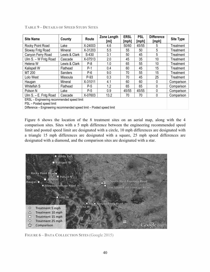
40

TABLE 9 – DETAILS OF SPEED STUDY SITES

Figure 6 shows the location of the 8 treatment sites on an aerial map, along with the 4 comparison sites. Sites with a 5 mph difference between the engineering recommended speed limit and posted speed limit are designated with a circle, 10 mph differences are designated with a triangle 15 mph differences are designated with a square, 25 mph speed differences are designated with a diamond, and the comparison sites are designated with a star.

FIGURE 6 – DATA COLLECTION SITES (Google 2015)

Site Name County Route Zone Length [mi]

ERSL [mph]

PSL [mph]

Difference [mph] Site Type

Rocky Point Road Lake X-24003 4.6 50/60 45/55 5 Treatment Sloway Fntg Road Mineral X-31203 5.5 55 50 5 Treatment Canyon Ferry Road Lewis & Clark S-430 3.1 50 45 5 Treatment Ulm S. – W Fntg Road Cascade X-07513 2.0 45 35 10 Treatment Helena W Lewis & Clark P-8 1.0 65 55 10 Treatment Kalispell W Flathead P-1 0.4 60 45 15 Treatment MT 200 Sanders P-6 9.0 70 55 15 Treatment Lolo West Missoula P-93 0.3 70 45 25 Treatment Haugan Mineral X-31011 4.1 60 60 0 Comparison Whitefish S Flathead P-5 1.2 65 65 0 Comparison Polson N Lake P-5 0.9 45/55 45/55 0 Comparison Ulm S. – E. Fntg Road Cascade X-07603 13.2 70 70 0 Comparison ERSL – Engineering recommended speed limit PSL – Posted speed limit Difference – Engineering recommended speed limit – Posted speed limit

41

Speed data were collected using Nu-metrics, Hi-star on-pavement sensors. These sensors measure 6.5 x 5.5 x 0.63 inches and were used because they are less conspicuous than other data collection equipment. A previous study compared the potential measurement errors of various speed collection devices and found these on-pavement sensors to provide accurate average speeds (Poe, Tarris, and Mason 1996b). All sensors were temporarily fastened to the asphalt pavement surface using a 22-caliber nail gun and covered using a black, rubber mat to further conceal it and protect it from traffic.

Four sensors were installed at each treatment site: two within the segment with a posted speed limit set lower than engineering recommendations and two outside of the segment. The two within the segment were placed either at the location previously used by MDT for speed data collection at these sites or the least-restrictive geometric feature to capture the highest operating speeds in both travel directions. The two sensors placed outside of the segment were designated as control sensors and used to capture operating speeds in both directions on the same roadway to account for daily fluctuations in the speed data. At comparison locations, a single detector was installed at the least-restrictive geometric feature to capture the highest speeds at these locations. Schematic drawings of the detector locations are provided in Appendix B for reference.

Speed data were collected at three different time periods at each site. Each of the three data collection trips represented a different level of speed enforcement present at the treatment and control locations:

July 20-23, 2015: no enforcement period August 10-13, 2015: light enforcement period October 26-29, 2015: heavy enforcement period.

The research team coordinated closely with the Montana Highway Patrol to ensure that the level of enforcement was consistent across all sites during these periods. During the no enforcement period, marked enforcement vehicles were not present at any of the treatment, control or comparison locations during the data collection period. During the light enforcement period, regular speed patrols were made at the treatment and control sites by marked enforcement vehicles during the data collection period. Enforcement vehicles were asked to stay clear of the comparison locations to provide a baseline with no enforcement. The heavy enforcement period consisted of either frequent patrols by enforcement vehicles or the presence of manned or unmanned vehicles parked within the study area at the treatment and control sites. Again, enforcement vehicles were asked to stay clear of the comparison locations to provide a baseline with no enforcement. The research team received verification of the presence of enforcement vehicles during the heavy enforcement period at only a few sites during the third data collection trip. These locations and time periods were:

Ulm SE Frontage Road: 10:30 AM – 12:30 PM Ulm SW Frontage Road: 12:20 PM – 1:50 PM

The research team differentiated these known heavy enforcement periods from other heavy enforcement periods to see if there was a difference in operating speeds between the two periods.

42

All sensors were installed for an 8-12 hour period at each site. Speed data were collected during daylight hours only. The following data were recorded from each sensor:

Timestamp of vehicle passage Vehicle length Vehicle speed Pavement temperature Pavement conditions (e.g., dry or wet)

DATA COMPILATION PROCESS Upon collecting the data, the research team examined all measured speed measurements and removed erroneous data that did not reflect free flow travel speeds at each site during each data collection period. The data compilation process consisted of four steps that are described in more detail below:

1. Identification and removal of incomplete observations 2. Identification and removal of vehicles affected by presence of other vehicles 3. Identification and removal of speeds from large vehicles 4. Identification and removal of speed outliers

In the first step, incomplete observations recorded by the speed sensors were removed. These were observations that were either missing the vehicle length or vehicle speeds. In the second step, observations with small headways were identified and removed. These observations represent vehicles whose travel speeds are likely to be influenced by the preceding vehicle (e.g., vehicles traveling in a platoon) and that might not be traveling in free flow. Based on a previous study (Mahoney et al, 2003), a critical headway of 4 seconds was identified as the threshold between free flow and non-free flow conditions. Vehicles with headways (identified using the timestamp) less than 4 seconds were removed from the dataset. In the third step, larger vehicles (those that were not likely to be passenger cars or single axle trucks) were identified and removed from the dataset. This was done since large vehicles typically travel at slower speeds and would introduce bias into the observed operating speeds on the roadway. A critical length of 20 feet was identified as the cutoff to identify larger trucks. Vehicles with a measured length larger than 20 feet were removed from the dataset.

In the fourth step, individual speed observations during each data collection period and at each measurement location were manually examined to identify outliers that might influence the speed results. For instance, a large number of low speeds were observed that did not seem indicative of free flow travel conditions. At some locations, speed data collection equipment had to be placed near driveways or other locations near which vehicles might be likely to slow down. Some of the measured speeds were up to 40 mph below the posted speed limit. Conversely, extremely high speeds were also observed in which vehicles traveled at up to 40 mph over the posted speed limit. These (few) low-speed and high-speed outliers were removed from the dataset to provide a more accurate depiction of realistic free flow travel speeds at the data

43

collection locations. Specifically, the research team removed measured speeds that were lower than 10 mph under the posted speed limit or 20 mph above the posted speed limit. The low-speed cutoff of 10 mph under the posted speed limit was selected because this seemed representative of the lowest free flow travel speed expected at the data collection locations. The high-speed cutoff was selected because 20 mph above the posted speed limit was considered the largest reasonable travel speeds expected. The low-speed observations removed represented about 6.6% of the measured speeds while the high-speed observations removed represented about 2.2% of the measured speeds.

CRASH DATA The research team requested and received electronic crash data from numerous sites in Montana with speed limits set lower than engineering recommendations (treatment sites) and with speed limits set equal to engineering recommendations (comparison sites). This crash data facilitated a comprehensive safety analysis that allowed the research team to develop models to estimate the safety effects of setting speed limits lower than engineering recommendations. Table 10 provides a summary of the data available to the research team for this analysis for treated sites (those with posted speed limits set lower than engineering recommendations) while Table 11 provides details for comparison sites (those with posted speed limits set equal to engineering recommendations).

44

TABLE 10 – DETAILS OF CRASH DATA AVAILABLE AT TREATED SITES

Site No. City Route Data PSL changed

Length [mi]

ERSL [mph]

PSL [mph]

Beginning of

Analysis Period

End of Analysis Period

Type

10101 Rocky Point Rd. X-24003 31-Jan-13 4.6 50/60 45/55 1-Jan-09 31-Dec-15 Treatment

10201 Kalispell W. P-1 6-Dec-07 0.4 60 45 1-Jan-04 1-Jul-14 Treatment 10301 Lolo West P-93 24-Mar-11 0.3 70 45 1-Jan-05 31-Dec-14 Treatment

10401 Sloway Fntg Rd X-31203 27-Sep-12 5.5 55 50 1-Jan-08 31-Dec-15 Treatment

10501 St Regis P-35 12-Feb-09 1.3 35/45/60 30/40/55 1-Jan-05 1-Jul-14 Treatment

10601 MT 200 (MP56-65) P-6 26-Sep-13 9.0 70 55 1-Jan-08 31-Dec-15 Treatment

10701 Valley Center Rd S-235 31-Oct-13 4.4 50 45 1-Jan-10 31-Dec-15 Treatment

10801 MT City-Clancy

S-282/X-22925 30-Apr-07 5.6 60 55 1-Jan-98 1-Jul-14 Treatment

10901 Continental Dr. U-1807 24-Mar-11 0.6 45 35 1-Jan-07 31-Dec-14 Treatment

11001 Helena W P-8 24-Feb-05 1.0 65 55 1-Jan-00 1-Jul-14 Treatment

11101 Canyon Ferry RD S-430 24-Apr-08 3.1 50 45 1-Jan-05 1-Jul-14 Treatment

11201 Cut Bank E P-1 29-Jul-10 0.3 35 25 1-Jan-06 1-Jul-14 Treatment

11301 ULM S - W FNTG Rd X-07513 29-Jul-10 2.0 45 35 1-Jan-06 1-Jul-14 Treatment

11401 Billings NW P-53 24-Apr-08 2.9 60 50 1-Jan-04 1-Jul-14 Treatment ERSL – Engineering recommended speed limit PSL – Posted speed limit

45

TABLE 11 – DETAILS OF CRASH DATA AVAILABLE AT REFERENCE SITES

County Site Route Length [mi]

ERSL [mph]

Beginning of Analysis Period

End of Analysis Period

Gallatin Amsterdam Rd S-347 2.2 55 1-Jan-05 1-Jul-14 Jefferson/LC Ashgrove Rd S-518 2.8 65 1-Jan-98 1-Jul-14 Yellowstone Blue Creek Rd S-416 3.4 50 1-Jan-09 1-Jul-14

Jefferson Boulder S P-69 0.9 45 1-Jan-05 1-Jul-14 Powder River Broadus E P-23 0.4 50 1-Jan-05 1-Jul-14

Lincoln Bull Lake P-56 3.3 55 1-Jan-08 1-Jul-14 Blaine Chinook P-1 0.6 30 1-Jan-08 1-Jul-14 Teton Choteau S P-3 0.7 30 1-Jan-05 1-Jul-14

Gallatin Cottonwood Rd S-345 3.0 55 1-Jan-05 1-Jul-14 Missoula East Broadway U-8112 1.0 45 1-Jan-07 1-Jul-14 Madison Ennis W P-29 1.3 60 1-Jan-05 1-Jul-14 Flathead Foys Lake S-503 9.9 30 1-Jan-09 1-Jul-14 Cascade Great Falls N P-10 1.2 55 1-Jan-04 1-Jul-14

Lewis & Clark Green Meadow Rd S-231 5.5 55 1-Jan-08 1-Jul-14 Ravalli Hamilton N P-7 1.7 65 1-Jan-00 1-Jul-14 Ravalli Hamilton S P-7 2.8 60 1-Jan-00 1-Jul-14 Mineral Haugan X-31011 4.1 60 1-Jan-07 1-Jul-14

Jefferson Jefferson City-Clancy X-22925 4.7 60 1-Jan-01 1-Jul-14 Yellowstone King Ave W/Buffalo Trail Rd S-532 10.5 60 1-Jan-08 1-Jul-14

Fergus Lewistown E P-57 0.4 55 1-Jan-05 1-Jul-14 Phillips Malta W P-1 0.2 35 1-Jan-06 1-Jul-14

Missoula Missoula SW P-7 5.9 65 1-Jan-04 1-Jul-14 Cascade NE Bypass (GE) U-5205 1.6 45 1-Jan-07 1-Jul-14 Cascade NW Bypass (GF) U-5206 0.9 45 1-Jan-07 1-Jul-14

Toole Oilmont W S-343 0.8 45 1-Jan-06 1-Jul-14 Lake Polson N P-5 0.9 70 1-Jan-10 1-Jul-14

Flathead Reserve Dr W S-548 2.8 55 1-Jan-08 1-Jul-14 Lincoln Rexford Area P-33 7.7 60 1-Jan-08 1-Jul-14

Yellowstone Rimrock Rd S-302 2.1 55 1-Jan-05 1-Jul-14 Missoula Salmon Lake N P-83 8.7 55 1-Jan-08 1-Jul-14

Toole Shelby W P-1 0.7 60 1-Jan-04 1-Jul-14 Mineral Tarkio X-31070 14.3 60 1-Jan-08 1-Jul-14

Missoula Turah-Clinton S-210 6.6 60 1-Jan-98 1-Jul-14 Cascade Ulm S - E Fntg Rd X-07603 13.2 70/45 1-Jan-06 1-Jul-14 Meagher White Sulphur S P-14 0.7 45/35/25 1-Jan-05 1-Jul-14 Flathead Whitefish NW P-5 3.1 60 1-Jan-04 1-Jul-14 Flathead Whitefish S P-5 1.2 65 1-Jan-00 1-Jul-14 Jefferson Whitehall E P-69 0.2 35 1-Jan-07 1-Jul-14

ERSL – Engineering recommended speed limit

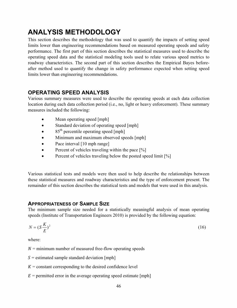
46

ANALYSIS METHODOLOGY This section describes the methodology that was used to quantify the impacts of setting speed limits lower than engineering recommendations based on measured operating speeds and safety performance. The first part of this section describes the statistical measures used to describe the operating speed data and the statistical modeling tools used to relate various speed metrics to roadway characteristics. The second part of this section describes the Empirical Bayes before-after method used to quantify the change in safety performance expected when setting speed limits lower than engineering recommendations.

OPERATING SPEED ANALYSIS Various summary measures were used to describe the operating speeds at each data collection location during each data collection period (i.e., no, light or heavy enforcement). These summary measures included the following:

Mean operating speed [mph] Standard deviation of operating speed [mph] 85th percentile operating speed [mph] Minimum and maximum observed speeds [mph] Pace interval [10 mph range] Percent of vehicles traveling within the pace [%] Percent of vehicles traveling below the posted speed limit [%]

Various statistical tests and models were then used to help describe the relationships between these statistical measures and roadway characteristics and the type of enforcement present. The remainder of this section describes the statistical tests and models that were used in this analysis.

APPROPRIATENESS OF SAMPLE SIZE The minimum sample size needed for a statistically meaningful analysis of mean operating speeds (Institute of Transportation Engineers 2010) is provided by the following equation:

2)(EKSN (16)

where:

= minimum number of measured free-flow operating speeds

= estimated sample standard deviation [mph]

= constant corresponding to the desired confidence level

= permitted error in the average operating speed estimate [mph]

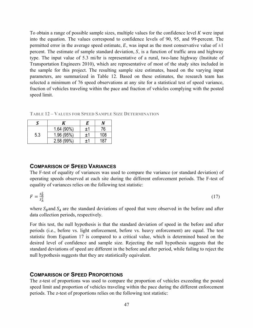
47

To obtain a range of possible sample sizes, multiple values for the confidence level were input into the equation. The values correspond to confidence levels of 90, 95, and 99-percent. The permitted error in the average speed estimate, , was input as the most conservative value of ±1 percent. The estimate of sample standard deviation, , is a function of traffic area and highway type. The input value of 5.3 mi/hr is representative of a rural, two-lane highway (Institute of Transportation Engineers 2010), which are representative of most of the study sites included in the sample for this project. The resulting sample size estimates, based on the varying input parameters, are summarized in Table 12. Based on these estimates, the research team has selected a minimum of 76 speed observations at any site for a statistical test of speed variance, fraction of vehicles traveling within the pace and fraction of vehicles complying with the posted speed limit.

TABLE 12 – VALUES FOR SPEED SAMPLE SIZE DETERMINATION

5.3 1.64 (90%) ±1 76 1.96 (95%) ±1 108 2.58 (99%) ±1 187

COMPARISON OF SPEED VARIANCES The F-test of equality of variances was used to compare the variance (or standard deviation) of operating speeds observed at each site during the different enforcement periods. The F-test of equality of variances relies on the following test statistic:

(17)

where and are the standard deviations of speed that were observed in the before and after data collection periods, respectively.

For this test, the null hypothesis is that the standard deviation of speed in the before and after periods (i.e., before vs. light enforcement, before vs. heavy enforcement) are equal. The test statistic from Equation 17 is compared to a critical value, which is determined based on the desired level of confidence and sample size. Rejecting the null hypothesis suggests that the standard deviations of speed are different in the before and after period, while failing to reject the null hypothesis suggests that they are statistically equivalent.

COMPARISON OF SPEED PROPORTIONS The z-test of proportions was used to compare the proportion of vehicles exceeding the posted speed limit and proportion of vehicles traveling within the pace during the different enforcement periods. The z-test of proportions relies on the following test statistic:

48

AA

AB

nnPP

PPZ11)1(

(18)

where PB and PA are the sample proportions from the before and after data collection periods, respectively; nB and nA are sample sizes for the corresponding proportions in the before and after periods; and, P is the combined proportion in both samples.

For this test, the null hypothesis is that the proportions in the before and after periods (i.e., before vs. light enforcement, before vs. heavy enforcement) are equal. The samples are assumed independent. The test statistic from Equation 18 is compared to a critical value, which is determined based on the desired level of confidence and sample size. Rejecting the null hypothesis indicates that the sample proportions differ, while failing to reject the null hypothesis indicates that the samples are equal.

MODELING OPERATING SPEEDS Analysis of variance (ANOVA) was used to examine the impacts of various roadway and enforcement characteristics—such as posted speed limit, difference between engineering recommended and posted speed limits, and presence of enforcement—on mean operating speeds. In general, ANOVA is used to test main and interaction effects of categorical independent variables on a dependent variable. The main objective of ANOVA is to determine if the group means formed by values of the independent variables differ significantly and thus influence the dependent variable. The assumptions of normality, homogeneity of variance and independent observations were evaluated using appropriate statistical tests and plots. Outliers were carefully evaluated to determine if they should be retained or excluded from the analysis. F-statistics for each factor included (main effects and interactions) in the ANOVA were assessed, and retained in the model if statistically significant. Multiple comparison tests were performed to identify which variables influenced operating speed and compliance data when a factor or interaction term was deemed statistically significant. These statistically significant factors were considered eligible to be included in the statistical models that were developed for:

Mean operating speed 85th percentile operating speed Compliance with the posted speed limit

The statistical modeling approach for each of these metrics is described below.

LINEAR REGRESSION MODELS FOR MEAN OPEARTING SPEEDS Linear regression was used to relate expected mean operating speed to the roadway characteristics considered in the ANOVA. This linear regression model is proposed as a prediction tool that will allow MDT engineers to estimate the expected mean operating speed at

49

other roadways in Montana based on their specific characteristics. Linear regression models take the form:

⋯ (19)

where are coefficients to be estimated, are observed explanatory variables associated with observation , is the dependent variable to be modeled and is the error term (a random error with a mean value of zero). In a linear model, the effects of all variables are assumed to be additive. That is, the change in any independent variable of one unit corresponds with an additive change in the prediction of the dependent variable by an amount equal to the associated model coefficient, . These model coefficients are typically estimated using the ordinary least squares procedure, which selects the coefficients that minimize errors between actual observations and those predicted by the model.

These models can provide the expected value (point estimate) of the independent variable for a given set of independent variables:

| ̅ ∑ . (20)

QUANTILE REGRESSION MODELS FOR 85TH PERCENTILE OPERATING SPEEDS Quantile regression was used to relate 85th percentile operating speeds to various roadway characteristics. Quantile models are similar to linear models in that they assume an additive relationship between the dependent and independent variables. However, while linear models can only be used to predict a mean value, quantile models can be used to predict any percentile value that is desired. In this report, we consider the 85th percentile speed at each of the data collection locations. The quantile model takes the same form as Equation 20 and coefficients are interpreted in a similar way; however, the model is estimated by selecting the parameters that minimize a weighted average of positive and negative error terms:

min∈ ∑

1∈ ∑

(21)

where is a number between 0 and 1 that represents the specific quantile being considered. All other notation is defined in relation to Equation 19.

LOGISTIC REGRESSION MODELS FOR SPEED LIMIT COMPLIANCE A binary logistic regression model was used to describe the probability that individual vehicles were observed traveling below the posted speed limit (i.e., speed limit compliance). The binary logistic regression model takes the following form:

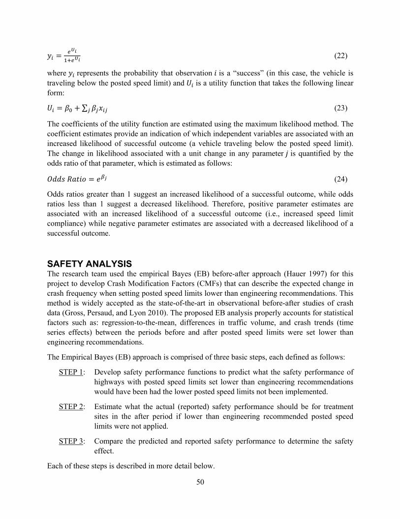
50

(22)

where represents the probability that observation is a “success” (in this case, the vehicle is traveling below the posted speed limit) and is a utility function that takes the following linear form:

∑ (23)

The coefficients of the utility function are estimated using the maximum likelihood method. The coefficient estimates provide an indication of which independent variables are associated with an increased likelihood of successful outcome (a vehicle traveling below the posted speed limit). The change in likelihood associated with a unit change in any parameter is quantified by the odds ratio of that parameter, which is estimated as follows:

(24)

Odds ratios greater than 1 suggest an increased likelihood of a successful outcome, while odds ratios less than 1 suggest a decreased likelihood. Therefore, positive parameter estimates are associated with an increased likelihood of a successful outcome (i.e., increased speed limit compliance) while negative parameter estimates are associated with a decreased likelihood of a successful outcome.

SAFETY ANALYSIS The research team used the empirical Bayes (EB) before-after approach (Hauer 1997) for this project to develop Crash Modification Factors (CMFs) that can describe the expected change in crash frequency when setting posted speed limits lower than engineering recommendations. This method is widely accepted as the state-of-the-art in observational before-after studies of crash data (Gross, Persaud, and Lyon 2010). The proposed EB analysis properly accounts for statistical factors such as: regression-to-the-mean, differences in traffic volume, and crash trends (time series effects) between the periods before and after posted speed limits were set lower than engineering recommendations.

The Empirical Bayes (EB) approach is comprised of three basic steps, each defined as follows:

STEP 1: Develop safety performance functions to predict what the safety performance of highways with posted speed limits set lower than engineering recommendations would have been had the lower posted speed limits not been implemented.

STEP 2: Estimate what the actual (reported) safety performance should be for treatment sites in the after period if lower than engineering recommended posted speed limits were not applied.

STEP 3: Compare the predicted and reported safety performance to determine the safety effect.

Each of these steps is described in more detail below.

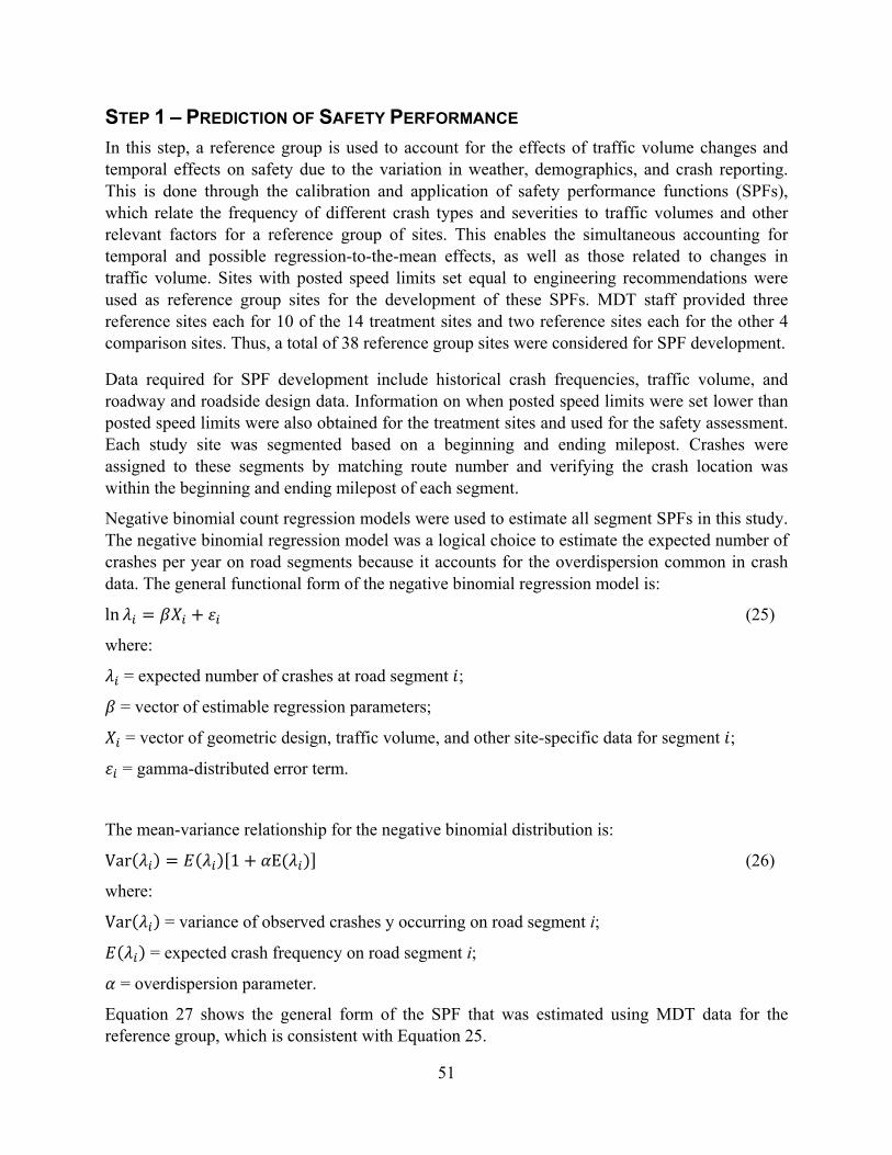
51

STEP 1 – PREDICTION OF SAFETY PERFORMANCE In this step, a reference group is used to account for the effects of traffic volume changes and temporal effects on safety due to the variation in weather, demographics, and crash reporting. This is done through the calibration and application of safety performance functions (SPFs), which relate the frequency of different crash types and severities to traffic volumes and other relevant factors for a reference group of sites. This enables the simultaneous accounting for temporal and possible regression-to-the-mean effects, as well as those related to changes in traffic volume. Sites with posted speed limits set equal to engineering recommendations were used as reference group sites for the development of these SPFs. MDT staff provided three reference sites each for 10 of the 14 treatment sites and two reference sites each for the other 4 comparison sites. Thus, a total of 38 reference group sites were considered for SPF development.

Data required for SPF development include historical crash frequencies, traffic volume, and roadway and roadside design data. Information on when posted speed limits were set lower than posted speed limits were also obtained for the treatment sites and used for the safety assessment. Each study site was segmented based on a beginning and ending milepost. Crashes were assigned to these segments by matching route number and verifying the crash location was within the beginning and ending milepost of each segment.

Negative binomial count regression models were used to estimate all segment SPFs in this study. The negative binomial regression model was a logical choice to estimate the expected number of crashes per year on road segments because it accounts for the overdispersion common in crash data. The general functional form of the negative binomial regression model is:

ln (25)

where:

= expected number of crashes at road segment ;

= vector of estimable regression parameters;

= vector of geometric design, traffic volume, and other site-specific data for segment ;

= gamma-distributed error term.

The mean-variance relationship for the negative binomial distribution is:

Var 1 E (26)

where:

Var = variance of observed crashes y occurring on road segment i;

= expected crash frequency on road segment i;

= overdispersion parameter.

Equation 27 shows the general form of the SPF that was estimated using MDT data for the reference group, which is consistent with Equation 25.

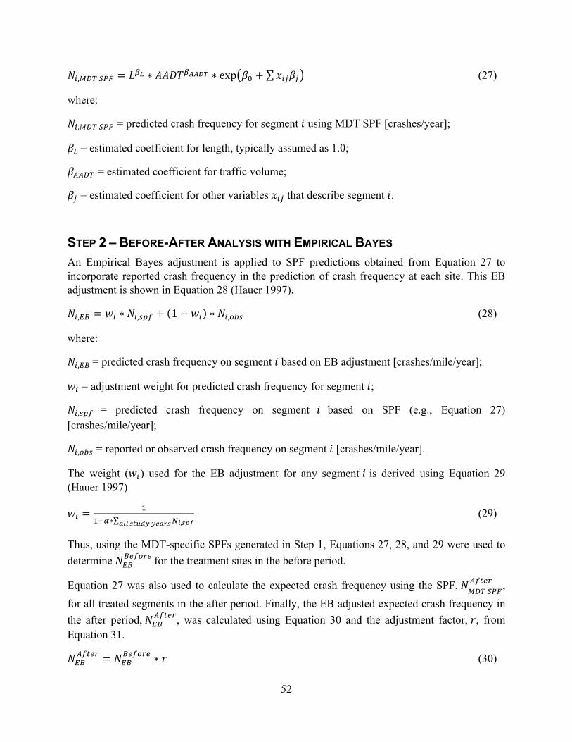
52

, ∗ ∗ exp ∑ (27)

where:

, = predicted crash frequency for segment using MDT SPF [crashes/year];

= estimated coefficient for length, typically assumed as 1.0;

= estimated coefficient for traffic volume;

= estimated coefficient for other variables that describe segment .

STEP 2 – BEFORE-AFTER ANALYSIS WITH EMPIRICAL BAYES An Empirical Bayes adjustment is applied to SPF predictions obtained from Equation 27 to incorporate reported crash frequency in the prediction of crash frequency at each site. This EB adjustment is shown in Equation 28 (Hauer 1997).

, ∗ , 1 ∗ , (28)

where:

, = predicted crash frequency on segment based on EB adjustment [crashes/mile/year];

= adjustment weight for predicted crash frequency for segment ;

, = predicted crash frequency on segment based on SPF (e.g., Equation 27) [crashes/mile/year];

, = reported or observed crash frequency on segment [crashes/mile/year].

The weight ( ) used for the EB adjustment for any segment is derived using Equation 29 (Hauer 1997)

∗∑ , (29)

Thus, using the MDT-specific SPFs generated in Step 1, Equations 27, 28, and 29 were used to determine for the treatment sites in the before period.

Equation 27 was also used to calculate the expected crash frequency using the SPF,

, for all treated segments in the after period. Finally, the EB adjusted expected crash frequency in the after period, , was calculated using Equation 30 and the adjustment factor, , from Equation 31.

∗ (30)

53

∑

∑

(31)

where:

= adjustment factor for differences in duration and traffic volume between before and after periods

= EB adjusted crash frequency prediction during the after period.

This EB adjusted value obtained from Equation 30 provides the expected crash frequency if no treatment was applied. This expected crash frequency is then compared with the reported crash frequency after the treatment was applied to assess the safety effects of the treatment.

STEP 3 – COMPARE PREDICTED AND ACTUAL SAFETY PERFORMANCE An unbiased estimate of the safety effect ( ) of the treatment or countermeasure is obtained using Equations 32 and 33.

(32)

∑ 1 (33)

where:

= unbiased estimate of safety effect of the countermeasure;

= reported or observed crashes on the segment during the after period.

Finally, the standard error associated with this safety effect estimate is then computed using Equations 34 and 35.

(34)

∑ (35)

54

RESULTS This section provides the results of the operating speed and safety analyses. First, the operating speed analysis is discussed. Then, the safety analysis is provided.

OPERATING SPEED ANALYSIS The operating speed analysis is divided into two parts. The first part provides the summary statistics of the speed data, including the statistical tests of equality between the no enforcement period and the light and heavy enforcement periods, respectively. The second provides the statistical models that can be used to relate the various roadway and enforcement characteristics to mean operating speed, 85th percentile operating speed and speed limit compliance.

SUMMARY STATISTICS OF SPEED DATA Summary statistics were calculated for observed speeds at each location and during each data collection period after the data were compiled as described earlier. The follow summary measures were determined:

Number of observations Mean operating speed (mph) Standard deviation of observed speeds (mph) 85th-percentile operating speed (mph) Minimum operating speed (mph) Maximum operating speed (mph) Pace interval (10 mph range) Percent of observations within pace Percent of observations traveling below posted speed limit

The summary statistics are provided in Table 13 through Table 15. Please note that the posted speed limits and engineering recommended speed limit values included in the tables for the control sites are values for the associated treatment sites (control points were on same roadway as treatment sites). Several sites did not have an adequate sample of observed operating speeds after the data cleaning and compilation process based on the minimum level of significance provided in Table 12; these sites are identified by the darker shaded rows in the tables. These sites include both treatment and control locations on Sloway Frontage Road (both direction) and Ulm SW Frontage Road (both direction), as well as the Ulm SE Frontage Road and Haugin comparison locations. These locations all represent extremely low-volume roads for which very few vehicles were observed during the data collection periods. The Lolo West WB control location also had very few observations during the heavy enforcement period. Although summary statistics are provided for these locations, care should be taken when using these summary statistics as they might not be fully representative of operating speeds at these sites.

The F-tests were performed to determine if the standard deviation of speed changed by a statistically significant amount at each of the sites from the no enforcement to the light and heavy enforcement periods, respectively. Statistically significant differences between the light or heavy

55

enforcement periods, relative to the no enforcement period, are noted in Table 14 and Table 15, respectively. All statistically significant differences were associated with a reduction in standard deviation of operating speed during one of the enforcement periods (relative to the no enforcement period). However, in most cases these reductions were less than 1 mph lower than the no enforcement period.

56

TABLE 13 – SUMMARY STATISTICS FOR OBSERVED SPEEDS DURING “NO ENFORCEMENT” PERIOD

Site Site Type PSL ERSL Direction Number of observations

Mean [mph]

Std.Dev [mph]

85th [mph]

Min [mph]

Max [mph]

Pace [mph]

% within Pace

% below PSL

Canyon Ferry Road Treatment 45 50 EB 1181 46.01 4.28 50 35 64 42 - 52 77.73 36.07 Canyon Ferry Road Treatment 45 50 WB 1484 43.88 4.18 48 35 65 39 - 49 78.64 59.23 Helena West Treatment 55 65 EB 1239 53.69 4.75 58 45 74 49 - 59 73.45 61.26 Helena West Treatment 55 65 WB 933 54.08 4.81 59 45 74 49 - 59 71.81 55.63 Kalispell W. Treatment 45 60 EB 1084 50.46 5.7 56 35 65 46 - 56 62.08 14.85 Kalispell W. Treatment 45 60 WB 1193 48.54 5.62 54 35 65 44 - 54 64.54 24.48 Lolo West Treatment 45 70 EB 393 48.34 6.26 55 35 65 41 - 51 55.73 30.03 Lolo West Treatment 45 70 WB 387 49.84 5.47 55 35 65 46 - 56 68.48 14.47 MT 200 Treatment 55 70 EB 249 59.64 5.61 65 45 75 54 - 64 71.08 13.25 MT 200 Treatment 55 70 WB 410 57.86 6.37 65 45 75 51 - 61 62.44 32.93 Rocky Point Rd Treatment 45 50 EB 526 47.35 5.26 53 35 63 42 - 52 68.63 32.13 Rocky Point Rd Treatment 45 50 WB 364 48.65 5.51 54 35 65 45 - 55 64.01 21.70 Sloway Frontage Road Treatment 50 55 EB 17 45.59 4.77 47 41 56 38 - 48 82.35 82.35 Sloway Frontage Road Treatment 50 55 WB 21 50.19 8.72 61 40 68 36 - 46 42.86 42.86 Ulm S W Frontage Road Treatment 35 45 EB 67 38.75 6.35 45 26 54 35 - 45 65.67 17.91 Ulm S W Frontage Road Treatment 35 45 WB 62 41.89 6.64 48 27 53 39 - 49 58.06 14.52 Canyon Ferry Road Control 45 50 EB 1253 45.93 4.72 50 35 65 41 - 51 75.34 41.98 Canyon Ferry Road Control 45 50 WB 795 49.02 5.25 54 35 65 43 - 53 67.55 19.5 Helena West Control 55 65 EB 575 60.33 6.42 67 45 75 56 - 66 56.87 19.13 Helena West Control 55 65 WB 784 57.32 5.68 63 45 74 53 - 63 61.86 31.63 Kalispell W. Control 45 60 EB 989 57.38 4.71 62 36 65 54 - 64 75.73 1.52 Kalispell W. Control 45 60 WB 331 54.49 4.88 59 38 64 50 - 60 75.23 4.23 Lolo West Control 45 70 EB 286 56.37 6.5 63 35 65 56 - 66 61.19 5.94 Lolo West Control 45 70 WB 626 56.6 6.46 63 35 65 56 - 66 63.42 5.43 MT 200 Control 55 70 EB 214 56.73 5.43 62 46 75 52 - 62 65.42 37.38 MT 200 Control 55 70 WB 410 57.81 5.51 64 45 75 52 - 62 67.56 27.80 Rocky Point Rd Control 45 50 EB 300 53.57 5.99 60 35 65 49 - 59 59.67 6.67 Rocky Point Rd Control 45 50 WB 201 55.26 6.21 61 35 65 53 - 63 67.66 7.96

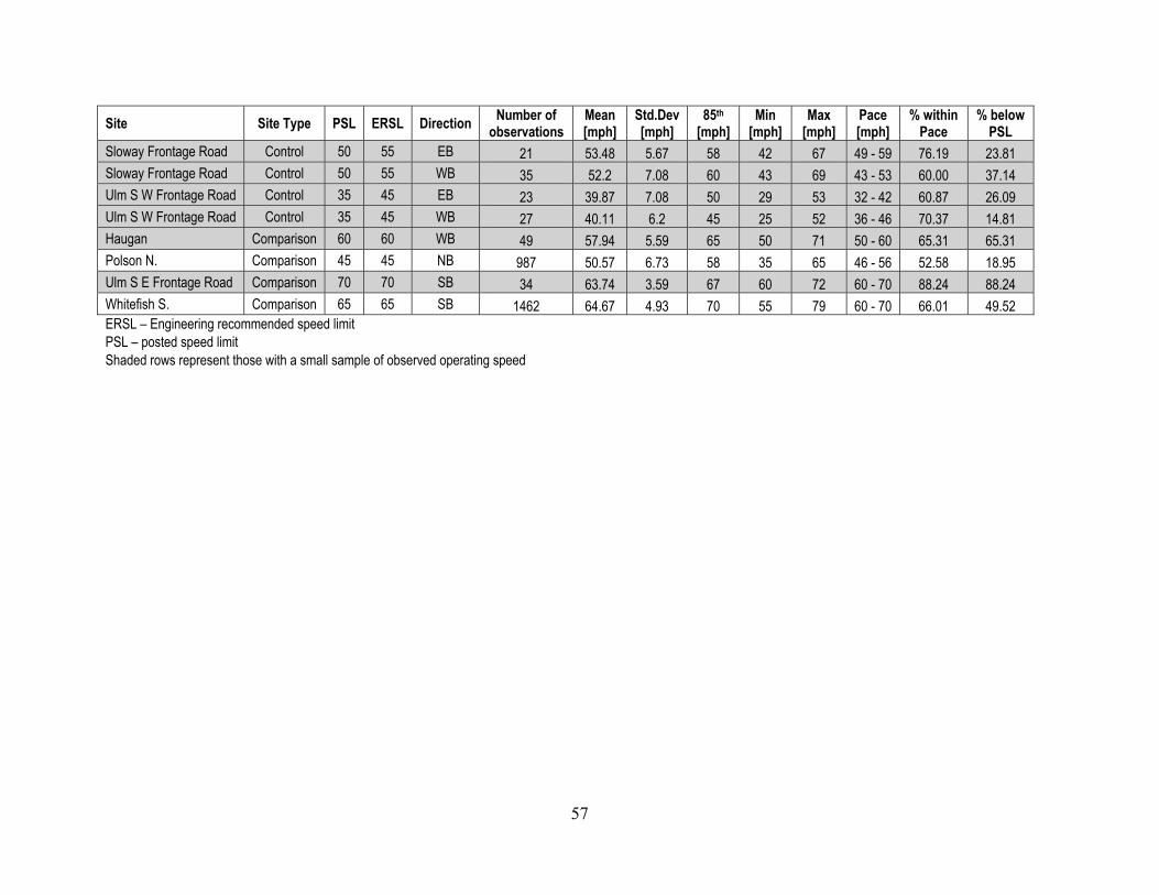
57


Mean [mph]

Std.Dev [mph]

85th [mph]

Min [mph]

Max [mph]

Pace [mph]

% within Pace

% below PSL

Sloway Frontage Road Control 50 55 EB 21 53.48 5.67 58 42 67 49 - 59 76.19 23.81 Sloway Frontage Road Control 50 55 WB 35 52.2 7.08 60 43 69 43 - 53 60.00 37.14 Ulm S W Frontage Road Control 35 45 EB 23 39.87 7.08 50 29 53 32 - 42 60.87 26.09 Ulm S W Frontage Road Control 35 45 WB 27 40.11 6.2 45 25 52 36 - 46 70.37 14.81 Haugan Comparison 60 60 WB 49 57.94 5.59 65 50 71 50 - 60 65.31 65.31 Polson N. Comparison 45 45 NB 987 50.57 6.73 58 35 65 46 - 56 52.58 18.95 Ulm S E Frontage Road Comparison 70 70 SB 34 63.74 3.59 67 60 72 60 - 70 88.24 88.24 Whitefish S. Comparison 65 65 SB 1462 64.67 4.93 70 55 79 60 - 70 66.01 49.52 ERSL – Engineering recommended speed limit PSL – posted speed limit Shaded rows represent those with a small sample of observed operating speed

58

TABLE 14 – SUMMARY STATISTICS FOR OBSERVED SPEEDS DURING “LIGHT ENFORCEMENT” PERIOD


Mean [mph]

Std.Dev [mph]

85th [mph]

Min [mph]

Max [mph]

Pace [mph]

% within Pace

% below PSL

Canyon Ferry Road Treatment 45 50 EB 1333 46.17 4.22 50 35 65 42 - 52 78.92 35.26 Canyon Ferry Road b Treatment 45 50 WB 1184 44.11 4.2 48 35 60 40 - 50 78.04 55.07 Helena West p, b Treatment 55 65 EB 1057 52.97 4.61 57 45 75 48 - 58 77.20 68.50 Helena West b Treatment 55 65 WB 940 55.64 5.04 60 45 75 50 - 60 69.57 41.28 Kalispell W. s, p Treatment 45 60 EB 1379 51.34 5.32 56 36 65 47 - 57 67.08 10.66 Kalispell W. s Treatment 45 60 WB 1558 48.47 5.14 54 35 65 43 - 53 67.27 22.21 Lolo West b Treatment 45 70 EB 539 46.09 6.02 52 35 65 40 - 50 61.60 44.34 Lolo West b Treatment 45 70 WB 664 47.59 5.46 53 35 65 43 - 53 64.01 28.77 MT 200 Treatment 55 70 EB 111 59.32 5.35 65 45 75 54 - 64 66.67 17.12 MT 200 s, b Treatment 55 70 WB 332 58.91 5.73 65 45 75 53 - 63 65.36 21.39 Rocky Point Rd b Treatment 45 50 EB 508 48.27 5.32 53 35 65 44 - 54 67.32 24.02 Rocky Point Rd Treatment 45 50 WB 422 49.18 5.42 55 36 65 44 - 54 66.11 19.19 Sloway Frontage Road Treatment 50 55 EB 20 53.5 7.57 63 41 68 49 - 59 60.00 25.00 Sloway Frontage Road Treatment 50 55 WB 15 50.53 7.07 59 40 62 44 - 54 53.33 46.67 Ulm S W Frontage Road Treatment 35 45 EB 11 39.45 4.89 44 31 45 36 - 46 81.82 18.18 Ulm S W Frontage Road Treatment 35 45 WB 22 39.73 5.74 45 27 48 39 - 49 63.64 27.27 Canyon Ferry Road s Control 45 50 EB 1402 45.7 4.43 50 35 65 41 - 51 77.25 42.01 Canyon Ferry Road b Control 45 50 WB 1384 47.61 5.28 53 35 64 42 - 52 66.55 27.38 Helena West s Control 55 65 EB 1048 59.63 5.94 66 45 75 55 - 65 60.5 19.37 Helena West b Control 55 65 WB 789 58.83 5.99 65 45 75 54 - 64 59.19 23.07 Kalispell W. Control 45 60 EB 1238 57.13 4.81 62 35 65 54 - 64 74.23 1.62 Kalispell W. p Control 45 60 WB 1426 54.54 5.15 60 35 65 51 - 61 67.60 3.37 Lolo West Control 45 70 EB 392 55.65 7.3 63 35 65 56 - 66 61.22 9.69 Lolo West p Control 45 70 WB 471 55.21 6.85 62 35 65 55 - 65 56.48 8.07 MT 200 p Control 55 70 EB 170 58.35 4.76 63 45 72 52 - 62 75.29 20.00 MT 200 s, p, b Control 55 70 WB 332 61.37 5.91 68 46 75 56 - 66 59.04 12.65 Rocky Point Rd Control 45 50 EB 276 54.41 5.81 60 37 65 49 - 59 64.13 5.07 Rocky Point Rd Control 45 50 WB 252 56.1 5.59 62 38 65 54 - 64 67.46 3.97

59


Mean [mph]

Std.Dev [mph]

85th [mph]

Min [mph]

Max [mph]

Pace [mph]

% within Pace

% below PSL

Sloway Frontage Road Control 50 55 EB 14 47.43 4.27 51 40 53 42 - 52 78.57 50.00 Sloway Frontage Road Control 50 55 WB 14 49.29 8.6 59 40 70 40 - 50 71.43 71.43 Ulm S W Frontage Road Control 35 45 EB 86 39.09 6.57 46 25 53 36 - 46 52.33 29.07 Ulm S W Frontage Road Control 35 45 WB 53 39.81 7.8 47 25 54 36 - 46 50.94 28.30 Haugan Comparison 60 60 WB 35 58.89 7.28 64 50 78 50 - 60 57.14 57.14 Polson N. s , p, b Comparison 45 45 NB 1252 50.86 6.1 57 35 65 47 - 57 60.86 15.65 Ulm S E Frontage Road Comparison 70 70 SB 60 65.08 4.26 69 60 75 60 - 70 86.67 86.67 Whitefish S. Comparison 65 65 EB 1637 64.78 4.81 70 55 79 60 - 70 68.97 46.43 ERSL – Engineering recommended speed limit PSL – posted speed limit Shaded rows represent those with a small sample of observed operating speed s – statistically significant difference between standard deviation of observed speeds compared to the “no enforcement” period p – statistically significant difference between percent of vehicles traveling within the pace compared to the “no enforcement” period b – statistically significant difference between percent of vehicles traveling below the posted speed limit compared to the “no enforcement” period

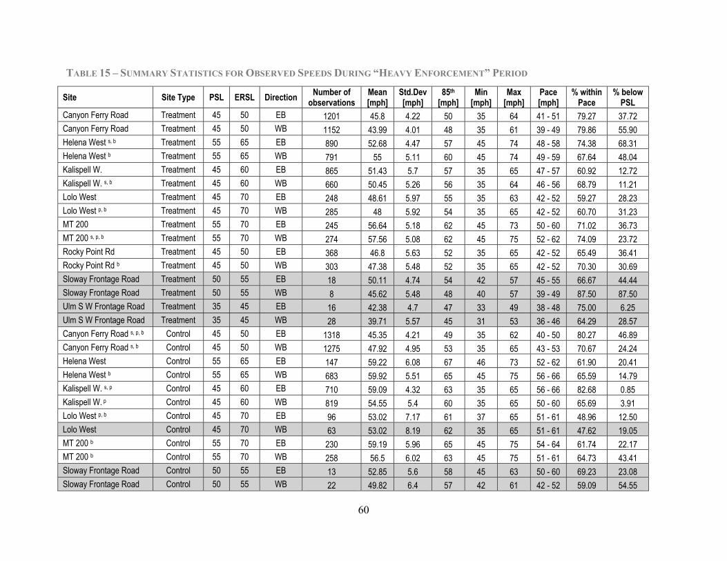
60

TABLE 15 – SUMMARY STATISTICS FOR OBSERVED SPEEDS DURING “HEAVY ENFORCEMENT” PERIOD


Mean [mph]

Std.Dev [mph]

85th [mph]

Min [mph]

Max [mph]

Pace [mph]

% within Pace

% below PSL

Canyon Ferry Road Treatment 45 50 EB 1201 45.8 4.22 50 35 64 41 - 51 79.27 37.72 Canyon Ferry Road Treatment 45 50 WB 1152 43.99 4.01 48 35 61 39 - 49 79.86 55.90 Helena West s, b Treatment 55 65 EB 890 52.68 4.47 57 45 74 48 - 58 74.38 68.31 Helena West b Treatment 55 65 WB 791 55 5.11 60 45 74 49 - 59 67.64 48.04 Kalispell W. Treatment 45 60 EB 865 51.43 5.7 57 35 65 47 - 57 60.92 12.72 Kalispell W. s, b Treatment 45 60 WB 660 50.45 5.26 56 35 64 46 - 56 68.79 11.21 Lolo West Treatment 45 70 EB 248 48.61 5.97 55 35 63 42 - 52 59.27 28.23 Lolo West p, b Treatment 45 70 WB 285 48 5.92 54 35 65 42 - 52 60.70 31.23 MT 200 Treatment 55 70 EB 245 56.64 5.18 62 45 73 50 - 60 71.02 36.73 MT 200 s, p, b Treatment 55 70 WB 274 57.56 5.08 62 45 75 52 - 62 74.09 23.72 Rocky Point Rd Treatment 45 50 EB 368 46.8 5.63 52 35 65 42 - 52 65.49 36.41 Rocky Point Rd b Treatment 45 50 WB 303 47.38 5.48 52 35 65 42 - 52 70.30 30.69 Sloway Frontage Road Treatment 50 55 EB 18 50.11 4.74 54 42 57 45 - 55 66.67 44.44 Sloway Frontage Road Treatment 50 55 WB 8 45.62 5.48 48 40 57 39 - 49 87.50 87.50 Ulm S W Frontage Road Treatment 35 45 EB 16 42.38 4.7 47 33 49 38 - 48 75.00 6.25 Ulm S W Frontage Road Treatment 35 45 WB 28 39.71 5.57 45 31 53 36 - 46 64.29 28.57 Canyon Ferry Road s, p, b Control 45 50 EB 1318 45.35 4.21 49 35 62 40 - 50 80.27 46.89 Canyon Ferry Road s, b Control 45 50 WB 1275 47.92 4.95 53 35 65 43 - 53 70.67 24.24 Helena West Control 55 65 EB 147 59.22 6.08 67 46 73 52 - 62 61.90 20.41 Helena West b Control 55 65 WB 683 59.92 5.51 65 45 75 56 - 66 65.59 14.79 Kalispell W. s, p Control 45 60 EB 710 59.09 4.32 63 35 65 56 - 66 82.68 0.85 Kalispell W. p Control 45 60 WB 819 54.55 5.4 60 35 65 50 - 60 65.69 3.91 Lolo West p, b Control 45 70 EB 96 53.02 7.17 61 37 65 51 - 61 48.96 12.50 Lolo West Control 45 70 WB 63 53.02 8.19 62 35 65 51 - 61 47.62 19.05 MT 200 b Control 55 70 EB 230 59.19 5.96 65 45 75 54 - 64 61.74 22.17 MT 200 b Control 55 70 WB 258 56.5 6.02 63 45 75 51 - 61 64.73 43.41 Sloway Frontage Road Control 50 55 EB 13 52.85 5.6 58 45 63 50 - 60 69.23 23.08 Sloway Frontage Road Control 50 55 WB 22 49.82 6.4 57 42 61 42 - 52 59.09 54.55

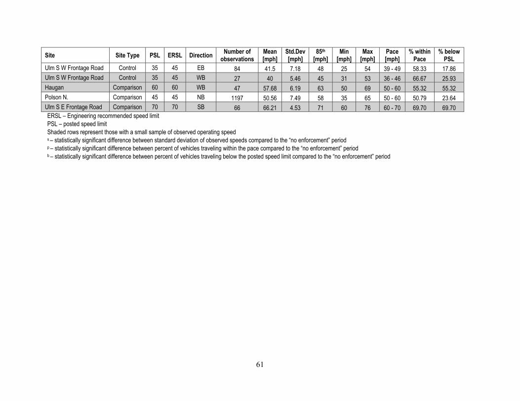
61


Mean [mph]

Std.Dev [mph]

85th [mph]

Min [mph]

Max [mph]

Pace [mph]

% within Pace

% below PSL

Ulm S W Frontage Road Control 35 45 EB 84 41.5 7.18 48 25 54 39 - 49 58.33 17.86 Ulm S W Frontage Road Control 35 45 WB 27 40 5.46 45 31 53 36 - 46 66.67 25.93 Haugan Comparison 60 60 WB 47 57.68 6.19 63 50 69 50 - 60 55.32 55.32 Polson N. Comparison 45 45 NB 1197 50.56 7.49 58 35 65 50 - 60 50.79 23.64 Ulm S E Frontage Road Comparison 70 70 SB 66 66.21 4.53 71 60 76 60 - 70 69.70 69.70 ERSL – Engineering recommended speed limit PSL – posted speed limit Shaded rows represent those with a small sample of observed operating speed s – statistically significant difference between standard deviation of observed speeds compared to the “no enforcement” period p – statistically significant difference between percent of vehicles traveling within the pace compared to the “no enforcement” period b – statistically significant difference between percent of vehicles traveling below the posted speed limit compared to the “no enforcement” period

62

Similarly, the percentage of vehicles traveling within the pace and below the posted speed limit were compared between the no enforcement period and the light and heavy enforcement periods, respectively, using the proportions test. Statistically significant differences between the light and heavy enforcement periods, relative to the no enforcement period, are noted n Table 14 and Table 15, respectively. For the percent of vehicles traveling within the pace, the range of statistically significant changes observed ranged from 12 percent fewer vehicles traveling within the pace (Lolo West control site during the heavy enforcement period) to 12 percent more vehicles traveling within the pace (MT 200 during the heavy enforcement period). For the percent of vehicles traveling below the posted speed limit, the range of statistically significant changes ranged between 17 percent fewer vehicles to 14 percent more vehicles during the light enforcement period, and 17 percent fewer vehicles to 23 percent more vehicles during the heavy enforcement period.

MODELS OF OPERATING SPEEDS AND SPEED LIMIT COMPLIANCE After the data cleaning and compilation process, a total of 55,845 unique speed observations were obtained from the entire set of treatment, control and comparison sites. These speed observations were put into a single analysis database to model the impacts of the following roadway characteristics on mean operating speed, 85th percentile operating speed and speed limit compliance:

Site type: treatment, control or comparison Enforcement type: none, light, heavy or known heavy Posted speed limit Difference between posted speed limit and engineering recommended speed limit

Table 16 provides summary statistics for each of these characteristics across the entire analysis dataset. As shown in Table 16, the majority of speed data were collected at treatment locations where the posted speed limit was set below the engineering recommended value. Most of these lower than engineering recommended speed limits were 5 to 15 mph below the engineering recommended value. The majority of posted speed limits were 45 or 55 mph. The level of enforcement was fairly balanced, although more data were collected during the no and light enforcement periods than the heavy enforcement period. Very few speeds were observed during the known heavy enforcement period, during which the Montana State Highway Patrol verified the presence of law enforcement at the data collection locations.

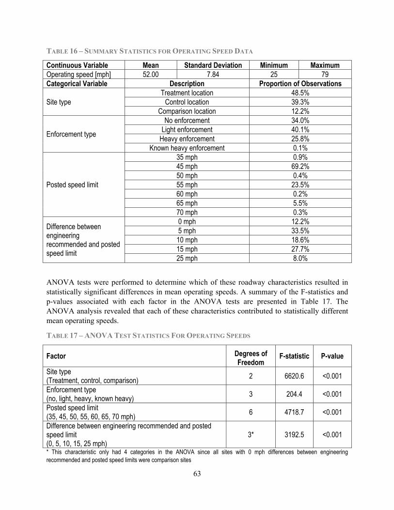
63

TABLE 16 – SUMMARY STATISTICS FOR OPERATING SPEED DATA

Continuous Variable Mean Standard Deviation Minimum Maximum Operating speed [mph] 52.00 7.84 25 79 Categorical Variable Description Proportion of Observations

Site type Treatment location 48.5%

Control location 39.3% Comparison location 12.2%

Enforcement type

No enforcement 34.0% Light enforcement 40.1%

Heavy enforcement 25.8% Known heavy enforcement 0.1%

Posted speed limit

35 mph 0.9% 45 mph 69.2% 50 mph 0.4% 55 mph 23.5% 60 mph 0.2% 65 mph 5.5% 70 mph 0.3%

Difference between engineering recommended and posted speed limit

0 mph 12.2% 5 mph 33.5% 10 mph 18.6% 15 mph 27.7% 25 mph 8.0%

ANOVA tests were performed to determine which of these roadway characteristics resulted in statistically significant differences in mean operating speeds. A summary of the F-statistics and p-values associated with each factor in the ANOVA tests are presented in Table 17. The ANOVA analysis revealed that each of these characteristics contributed to statistically different mean operating speeds.

TABLE 17 – ANOVA TEST STATISTICS FOR OPERATING SPEEDS

Factor Degrees of Freedom

F-statistic P-value

Site type (Treatment, control, comparison) 2 6620.6 <0.001

Enforcement type (no, light, heavy, known heavy) 3 204.4 <0.001

Posted speed limit (35, 45, 50, 55, 60, 65, 70 mph) 6 4718.7 <0.001

Difference between engineering recommended and posted speed limit (0, 5, 10, 15, 25 mph)

3* 3192.5 <0.001

* This characteristic only had 4 categories in the ANOVA since all sites with 0 mph differences between engineering recommended and posted speed limits were comparison sites

64

Based on these findings, a linear regression model was developed to relate mean operating speed to each of the roadway characteristics that had a statistically significant impact on mean operating speeds. All variables were included in the model as indicator variables that took the value of 1 if the characteristic was present and 0 if the characteristic was not present. The model was then refined by eliminating independent variables that were not statistically significant at the 95 percent confidence level. The final model output is provided in Table 18. The base conditions for the final model were:

Comparison location No enforcement or light enforcement Posted speed limit 45 mph or lower Posted speed limit equal to engineering recommended speed limit

TABLE 18 – LINEAR REGRESSION MODELING OUTPUT FOR MEAN OPERATING SPEEDS

Variable Coefficient Standard Error

t-statistic

p-value

Constant 50.8 0.10 508.1 <0.001 Control location 4.0 0.05 76.8 <0.001 Heavy enforcement -0.3 0.06 -5.5 <0.001 Known heavy enforcement -4.6 0.85 -5.4 <0.001 Posted speed limit of 50 or 55 mph 7.1 0.10 72.0 <0.001 Posted speed limit of 60, 65 or 75 mph 13.7 0.14 98.0 <0.001 5 mph difference in engineering recommended and posted speed limit -5.9 0.11 -54.1 <0.001

10 mph difference in engineering recommended and posted speed limit of 10 mph -3.8 0.15 -25.6 <0.001

15 or 25 mph difference in engineering recommended and posted speed limit -0.3 0.11 -3.0 0.002

Adjusted R2 = 0.4626

The model output in Table 18 suggests that operating speeds are generally higher at control locations than comparison locations. As expected, operating speeds were higher at locations with higher posted speed limits. Consistent with engineering expectation, enforcement was found to be associated with lower operating speeds. This effect was modest for locations where enforcement was not verified but practically significant for locations where known heavy enforcement took place. Light enforcement was found to have no statistically significant association with observed operating speeds. Finally, operating speeds were found to be lower at treatment locations for which posted speed limits were less than engineering recommended speed limits. The magnitude of the operating speed difference is greatest when the difference between the engineering recommended and actual posted speed limit is smallest, relative to the baseline condition of no difference between the engineering recommended speed limit and actual posted speed limit. Intuitively, this suggests that drivers obey the lower than engineering recommended

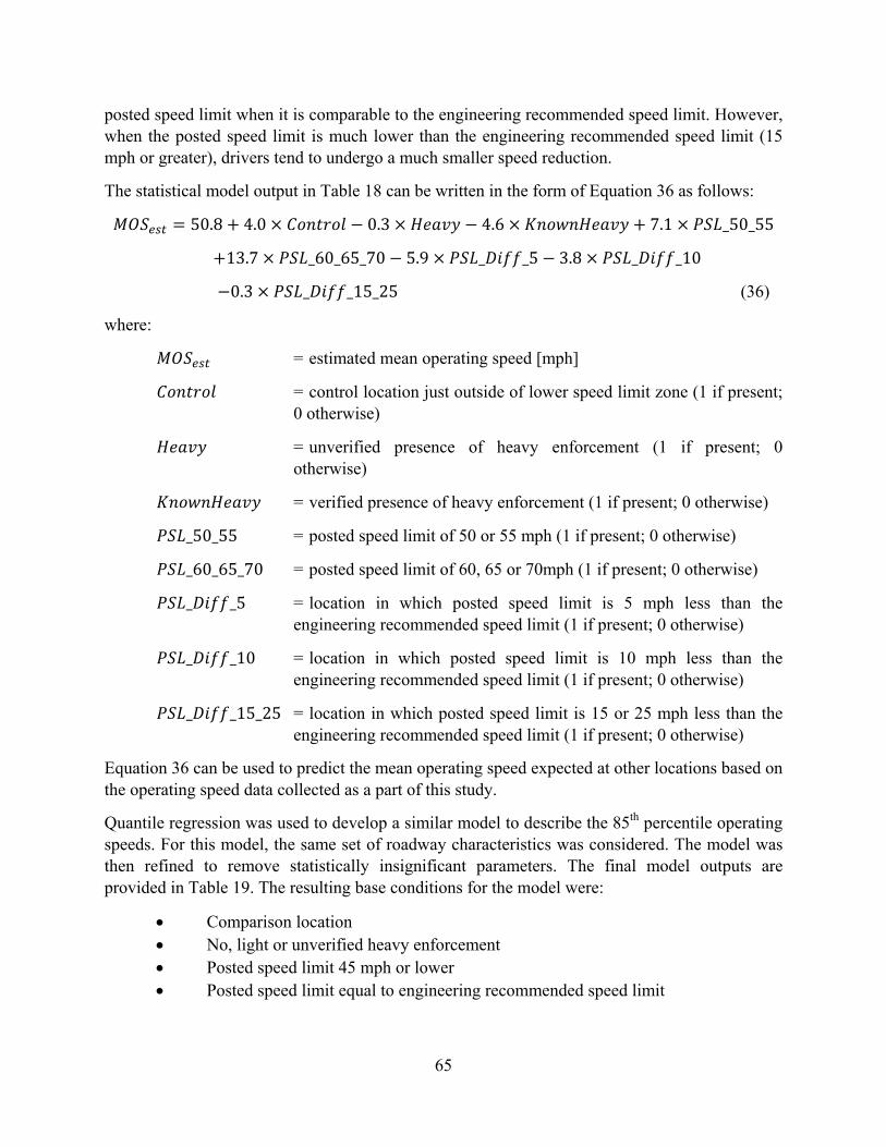
65

posted speed limit when it is comparable to the engineering recommended speed limit. However, when the posted speed limit is much lower than the engineering recommended speed limit (15 mph or greater), drivers tend to undergo a much smaller speed reduction.

The statistical model output in Table 18 can be written in the form of Equation 36 as follows:

50.8 4.0 0.3 4.6 7.1 _50_55

13.7 _60_65_70 5.9 _ _5 3.8 _ _10

0.3 _ _15_25 (36)

where:

= estimated mean operating speed [mph]

= control location just outside of lower speed limit zone (1 if present; 0 otherwise)

= unverified presence of heavy enforcement (1 if present; 0 otherwise)

= verified presence of heavy enforcement (1 if present; 0 otherwise)

_50_55 = posted speed limit of 50 or 55 mph (1 if present; 0 otherwise)

_60_65_70 = posted speed limit of 60, 65 or 70mph (1 if present; 0 otherwise)

_ _5 = location in which posted speed limit is 5 mph less than the engineering recommended speed limit (1 if present; 0 otherwise)


_ _15_25 = location in which posted speed limit is 15 or 25 mph less than the engineering recommended speed limit (1 if present; 0 otherwise)

Equation 36 can be used to predict the mean operating speed expected at other locations based on the operating speed data collected as a part of this study.

Quantile regression was used to develop a similar model to describe the 85th percentile operating speeds. For this model, the same set of roadway characteristics was considered. The model was then refined to remove statistically insignificant parameters. The final model outputs are provided in Table 19. The resulting base conditions for the model were:

Comparison location No, light or unverified heavy enforcement Posted speed limit 45 mph or lower Posted speed limit equal to engineering recommended speed limit

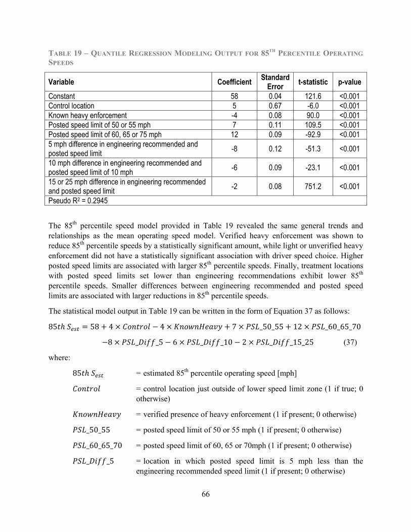
66

TABLE 19 – QUANTILE REGRESSION MODELING OUTPUT FOR 85TH PERCENTILE OPERATING SPEEDS

Variable Coefficient Standard Error t-statistic p-value

Constant 58 0.04 121.6 <0.001 Control location 5 0.67 -6.0 <0.001 Known heavy enforcement -4 0.08 90.0 <0.001 Posted speed limit of 50 or 55 mph 7 0.11 109.5 <0.001 Posted speed limit of 60, 65 or 75 mph 12 0.09 -92.9 <0.001 5 mph difference in engineering recommended and posted speed limit -8 0.12 -51.3 <0.001

10 mph difference in engineering recommended and posted speed limit of 10 mph -6 0.09 -23.1 <0.001

15 or 25 mph difference in engineering recommended and posted speed limit -2 0.08 751.2 <0.001

Pseudo R2 = 0.2945

The 85th percentile speed model provided in Table 19 revealed the same general trends and relationships as the mean operating speed model. Verified heavy enforcement was shown to reduce 85th percentile speeds by a statistically significant amount, while light or unverified heavy enforcement did not have a statistically significant association with driver speed choice. Higher posted speed limits are associated with larger 85th percentile speeds. Finally, treatment locations with posted speed limits set lower than engineering recommendations exhibit lower 85th percentile speeds. Smaller differences between engineering recommended and posted speed limits are associated with larger reductions in 85th percentile speeds.

The statistical model output in Table 19 can be written in the form of Equation 37 as follows:

85 58 4 4 7 _50_55 12 _60_65_70

8 _ _5 6 _ _10 2 _ _15_25 (37)

where:

85 = estimated 85th percentile operating speed [mph]

= control location just outside of lower speed limit zone (1 if true; 0 otherwise)

= verified presence of heavy enforcement (1 if present; 0 otherwise)

_50_55 = posted speed limit of 50 or 55 mph (1 if present; 0 otherwise)

_60_65_70 = posted speed limit of 60, 65 or 70mph (1 if present; 0 otherwise)


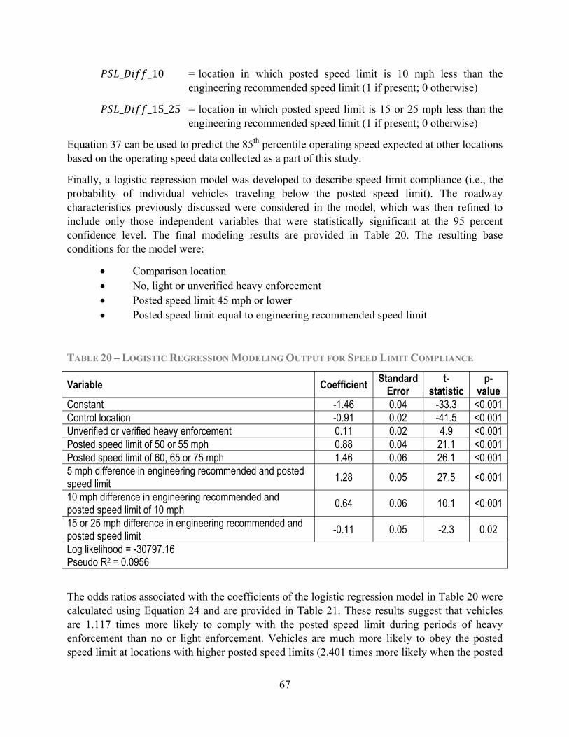
67


_ _15_25 = location in which posted speed limit is 15 or 25 mph less than the engineering recommended speed limit (1 if present; 0 otherwise)

Equation 37 can be used to predict the 85th percentile operating speed expected at other locations based on the operating speed data collected as a part of this study.

Finally, a logistic regression model was developed to describe speed limit compliance (i.e., the probability of individual vehicles traveling below the posted speed limit). The roadway characteristics previously discussed were considered in the model, which was then refined to include only those independent variables that were statistically significant at the 95 percent confidence level. The final modeling results are provided in Table 20. The resulting base conditions for the model were:

Comparison location No, light or unverified heavy enforcement Posted speed limit 45 mph or lower Posted speed limit equal to engineering recommended speed limit

TABLE 20 – LOGISTIC REGRESSION MODELING OUTPUT FOR SPEED LIMIT COMPLIANCE

Variable Coefficient Standard Error

t-statistic

p-value

Constant -1.46 0.04 -33.3 <0.001 Control location -0.91 0.02 -41.5 <0.001 Unverified or verified heavy enforcement 0.11 0.02 4.9 <0.001 Posted speed limit of 50 or 55 mph 0.88 0.04 21.1 <0.001 Posted speed limit of 60, 65 or 75 mph 1.46 0.06 26.1 <0.001 5 mph difference in engineering recommended and posted speed limit 1.28 0.05 27.5 <0.001

10 mph difference in engineering recommended and posted speed limit of 10 mph 0.64 0.06 10.1 <0.001

15 or 25 mph difference in engineering recommended and posted speed limit -0.11 0.05 -2.3 0.02

Log likelihood = -30797.16 Pseudo R2 = 0.0956

The odds ratios associated with the coefficients of the logistic regression model in Table 20 were calculated using Equation 24 and are provided in Table 21. These results suggest that vehicles are 1.117 times more likely to comply with the posted speed limit during periods of heavy enforcement than no or light enforcement. Vehicles are much more likely to obey the posted speed limit at locations with higher posted speed limits (2.401 times more likely when the posted

68

speed limit is 50 or 55 mph compared with the base case of less than 50 mph and 4.285 more likely when the posted speed limit is between 60 and 70 mph). Vehicles are also more likely to obey the posted speed limit at treatment locations for which the posted speed limit is only 5 or 10 mph less than the engineering recommended speed limit. When the posted speed limit is 15 mph or more lower than the engineering recommended speed limit, vehicles are more likely to travel in excess of the posted speed limit. These findings are consistent with the mean operating speed and 85th percentile operating speed models presented earlier.

TABLE 21 – ODDS RATIOS ASSOCIATED WITH LOGISTIC REGRESSION OUTPUT

Variable Odds Ratio Control location 0.402 Unverified or verified heavy enforcement 1.117 Posted speed limit of 50 or 55 mph 2.401 Posted speed limit of 60, 65 or 75 mph 4.285 5 mph difference in engineering recommended and posted speed limit 3.604 10 mph difference in engineering recommended and posted speed limit of 10 mph 1.887 15 or 25 mph difference in engineering recommended and posted speed limit 0.892

SAFETY ANALYSIS The safety analysis is divided into two parts. The first part provides the summary statistics of the safety data, including mean annual crash frequencies and crash rates for total and fatal + injury crashes. The second provides the results of the Empirical Bayes analysis and the associated crash modification factors for the practice of setting speed limits lower than engineering recommendations.

SUMMARY STATISTICS OF CRASH DATA The research team merged the available crash data to existing roadway inventory data to facilitate the safety analyses. The average annual daily traffic, total and fatal + injury crash frequencies, and total and fatal + injury crash rates for the treatment and reference group sites are shown in Table 22 and Table 23, respectively.

69

TABLE 22 – SUMMARY OF CRASH FREQUENCY AND CRASH RATES FOR TREATMENT SITES

Site Route # of years

Mean AADT

[veh/day]

Mean total crashes

[crash/yr]

Crash rate for total crashes

[crash/mil. VMT]

Mean fatal + injury crashes

[crash/yr]

Crash rate for fatal +

injury crashes

[crash/mil. VMT]

Before implementation of speed limit lower than engineering recommendations Billings NW P-53 4 3384 3.3 0.91 2.0 0.56 Canyon Ferry Rd S-430 3 3070 8.7 2.67 4.0 1.23 Continental Dr U-1807 4 4990 0.0 0.00 0.0 0.00 Cut Bank E P-1 4 1889 0.0 0.00 0.0 0.00 Helena West P-8 5 4338 4.4 2.78 0.0 0.00 Kalispell W P-1 3 6553 2.3 2.44 0.7 0.70 Lolo West P-93 6 2561 1.2 4.17 0.5 1.78 MT 200 P-6 5 1528 7.0 1.39 2.4 0.48 MT City-Clancy S-282/X-22925 9 773 4.4 2.81 0.9 0.56 Rocky Point Rd X-24003 4 1385 2.8 1.18 1.3 0.54 Sloway Fntg Rd X-31203 4 90 0.5 2.77 0.0 0.00 St Regis P-35 4 2776 1.8 1.23 0.8 0.53 Ulm S - W Fntg Rd X-07513 4 100 0.8 11.11 0.5 7.40 Valley Center Rd* S-235 3 2550 1.33 0.33 0.66 0.16

After implementation of speed limit lower than engineering recommendations Billings NW P-53 6 4108 3.2 0.73 1.7 0.38 Canyon Ferry Rd S-430 6 4335 3.0 0.65 1.2 0.26 Continental Dr U-1807 3 5063 0.0 0.00 0.0 0.00 Cut Bank E P-1 4 2408 0.0 0.00 0.0 0.00 Helena West P-8 9 6174 4.3 1.92 0.7 0.30 Kalispell W P-1 7 8211 0.9 0.72 0.1 0.12 Lolo West P-93 3 2793 1.3 4.25 0.7 2.19 MT 200 P-6 2 1684 7.6 1.37 4.0 0.72 MT City-Clancy S-282/X-22925 7 1123 2.3 1.00 0.7 0.31 Rocky Point Rd X-24003 2 1323 2.0 0.90 0.0 0.00 Sloway Fntg Rd X-31203 3 90 0.0 0.00 0.0 0.00 St Regis P-35 5 2624 1.2 0.89 0.4 0.30 Ulm S - W Fntg Rd X-07513 4 100 0.0 0.00 0.0 0.00 Valley Center Rd S-235 2 3460 2.5 0.45 1.0 0.18

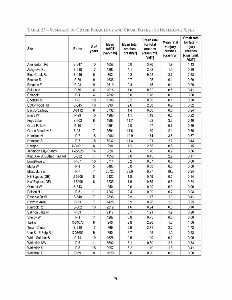
70

TABLE 23 – SUMMARY OF CRASH FREQUENCY AND CRASH RATES FOR REFERENCE SITES

Site Route # of years

Mean AADT

[veh/day]

Mean total crashes

[crash/yr]

Crash rate for total crashes

[crash/mil. VMT]

Mean fatal + injury crashes

[crash/yr]

Crash rate for fatal +

injury crashes

[crash/mil. VMT]

Amsterdam Rd S-347 10 1658 5.0 3.76 1.9 1.43 Ashgrove Rd S-518 17 1362 4.1 2.92 1.1 0.80 Blue Creek Rd S-416 6 802 9.2 9.22 2.7 2.68 Boulder S P-69 9 1636 0.7 1.25 0.1 0.20 Broadus E P-23 9 2610 0.4 1.15 0.1 0.29 Bull Lake P-56 6 1016 1.0 0.82 0.5 0.41 Chinook P-1 4 2892 0.8 1.18 0.0 0.00 Choteau S P-3 10 1305 0.2 0.60 0.1 0.30 Cottonwood Rd S-345 10 999 2.6 2.38 0.9 0.82 East Broadway U-8112 8 5732 1.4 0.66 0.5 0.24 Ennis W P-29 10 1960 1.1 1.18 0.2 0.22 Foys Lake S-503 6 1993 11.7 1.62 3.3 0.46 Great Falls N P-10 11 4261 2.0 1.07 0.6 0.29 Green Meadow Rd S-231 7 3594 11.6 1.60 2.1 0.30 Hamilton N P-7 15 10061 10.9 1.74 3.5 0.57 Hamilton S P-7 15 6032 11.8 1.91 2.7 0.44 Haugan X-31011 8 290 1.1 2.58 0.5 1.15 Jefferson City-Clancy X-22925 14 220 0.6 1.70 0.2 0.56 King Ave W/Buffalo Trail Rd S-532 7 4358 7.6 0.45 2.9 0.17 Lewistown E P-57 10 3714 0.2 0.37 0.0 0.00 Malta W P-1 5 3493 0.0 0.00 0.0 0.00 Missoula SW P-7 11 20725 39.0 0.87 10.6 0.24 NE Bypass (GE) U-5205 8 6122 1.8 0.49 0.5 0.14 NW Bypass (GF) U-5206 8 6235 1.6 0.79 0.5 0.24 Oilmont W S-343 1 250 0.0 0.00 0.0 0.00 Polson N P-5 11 7262 2.4 0.99 0.2 0.08 Reserve Dr W S-548 7 2396 2.9 1.17 1.0 0.41 Rexford Area P-33 7 1425 3.9 0.96 1.0 0.25 Rimrock Rd S-302 10 2212 1.6 0.94 0.3 0.18 Salmon Lake N P-83 7 2117 8.1 1.21 1.9 0.28 Shelby W P-1 11 4267 0.8 0.75 0.0 0.00 Tarkio X-31070 6 240 2.8 2.26 1.3 1.06 Turah-Clinton S-210 17 769 6.9 3.71 3.2 1.72 Ulm S - E Fntg Rd X-07603 9 390 3.7 1.95 1.0 0.53 White Sulphur S P-14 10 1628 0.5 1.20 0.0 0.00 Whitefish NW P-5 11 6692 6.1 0.80 2.6 0.34 Whitefish S P-5 15 9957 5.2 1.19 1.8 0.41 Whitehall E P-69 8 1629 0.0 0.00 0.0 0.00

71

EMPIRICAL-BAYES BEFORE-AFTER ANALYSIS

STEP 1 – PREDICTION OF FUTURE SAFETY PERFORMANCE The reference site data shown in Table 23 were used to develop SPFs to predict total and fatal + injury crash frequency for inclusion in the Empirical Bayes (EB) evaluation. A total of 409 unique roadway segments were available for the development of these SPFs: 376 for 2-lane roadway segments and 33 for 4-lane roadway segments. Because multiple years (between 1 and 17) of crash data were available for each location, the analysis database consisted of 3,053 total observations for 2-lane roadway segments and 382 total observations for 4-lane roadway segments. Table 24 and Table 25 show summary statistics for the 2-lane and 4-lane roadway segments, respectively. As shown in these tables, there are more property damage only crashes than fatal + injury crashes per year per segment. Traffic volumes are generally higher on 4-lane roadway segments than 2-lane roadway segments, as expected. Posted speed limits range from 25 to 70 mph, with 60 and 65 mph being the most common posted speed limits observed.

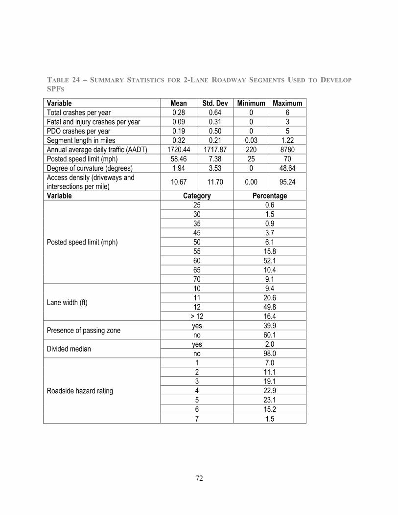
72

TABLE 24 – SUMMARY STATISTICS FOR 2-LANE ROADWAY SEGMENTS USED TO DEVELOP SPFS

Variable Mean Std. Dev Minimum Maximum Total crashes per year 0.28 0.64 0 6 Fatal and injury crashes per year 0.09 0.31 0 3 PDO crashes per year 0.19 0.50 0 5 Segment length in miles 0.32 0.21 0.03 1.22 Annual average daily traffic (AADT) 1720.44 1717.87 220 8780 Posted speed limit (mph) 58.46 7.38 25 70 Degree of curvature (degrees) 1.94 3.53 0 48.64 Access density (driveways and intersections per mile) 10.67 11.70 0.00 95.24

Variable Category Percentage

Posted speed limit (mph)

25 0.6 30 1.5 35 0.9 45 3.7 50 6.1 55 15.8 60 52.1 65 10.4 70 9.1

Lane width (ft)

10 9.4 11 20.6 12 49.8

> 12 16.4

Presence of passing zone yes 39.9 no 60.1

Divided median yes 2.0 no 98.0

Roadside hazard rating

1 7.0 2 11.1 3 19.1 4 22.9 5 23.1 6 15.2 7 1.5

73

TABLE 25 – SUMMARY STATISTICS FOR 4-LANE ROADWAY SEGMENTS USED TO DEVELOP SPFS

Variable Mean Std. Dev Minimum Maximum Total crashes per year 2.38 2.45 0 14 Fatal and injury crashes per year 0.68 1.11 0 10 PDO crashes per year 1.70 1.82 0 9 Segment length in miles 0.47 0.27 0.16 1.20 Annual average daily traffic (AADT) 12057.13 7505.99 649 2524 Posted speed limit (mph) 60.00 7.24 45 65 Degree of curvature (degrees) 1.53 2.11 0.00 7.07 Access density (driveways and intersections per mile) 14.62 14.82 0.00 83.87

Variable Category Percentage

Posted speed limit (mph)

45 13.5 50 7.7 60 22.7 65 56.1

Lane width (ft) 12 3.1 >12 96.9

Divided median yes 90.4 no 9.6

Roadside hazard rating

1 0.0 2 4.1 3 20.7 4 33.4 5 32.6 6 9.1 7 0.0

Based on the data available, SPFs were developed for 2-lane and 4-lane roadway segments separately, since the research team expected different relationships between crash frequency and the various roadway characteristics on these two unique roadway types. Two SPFs were developed for each: one SPF for total crash frequency and one SPF for combined fatal + injury crash frequency. Each of the characteristics included in Table 24 and Table 25 with sufficient variability in observations were included in the SPFs. All SPFs were in the form of Equation 27 above. Those variables with the expected sign that were either statistically significant ( 0.05) or marginally significant (0.05 0.30 ) were retained in the final model. Categorical variables were also combined into larger groupings where appropriate (e.g., similar regression coefficients for adjacent categories or to increase the sample size of among categories). For example, adjacent roadside hazard ratings were combined due to insufficient number of observations within each individual category or if similar safety trends were apparent across individual or combined categories.

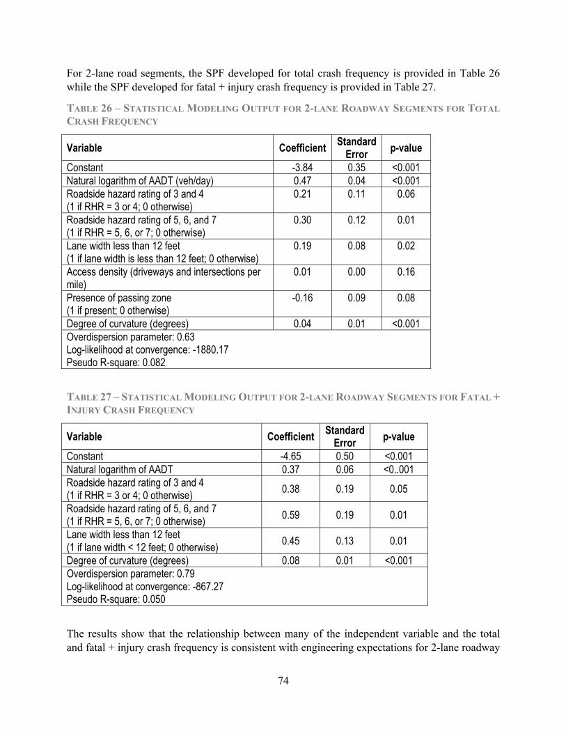
74

For 2-lane road segments, the SPF developed for total crash frequency is provided in Table 26 while the SPF developed for fatal + injury crash frequency is provided in Table 27.

TABLE 26 – STATISTICAL MODELING OUTPUT FOR 2-LANE ROADWAY SEGMENTS FOR TOTAL CRASH FREQUENCY

Variable Coefficient Standard Error p-value

Constant -3.84 0.35 <0.001 Natural logarithm of AADT (veh/day) 0.47 0.04 <0.001 Roadside hazard rating of 3 and 4 (1 if RHR = 3 or 4; 0 otherwise)

0.21 0.11 0.06

Roadside hazard rating of 5, 6, and 7 (1 if RHR = 5, 6, or 7; 0 otherwise)

0.30 0.12 0.01

Lane width less than 12 feet (1 if lane width is less than 12 feet; 0 otherwise)

0.19 0.08 0.02

Access density (driveways and intersections per mile)

0.01 0.00 0.16

Presence of passing zone (1 if present; 0 otherwise)

-0.16 0.09 0.08

Degree of curvature (degrees) 0.04 0.01 <0.001 Overdispersion parameter: 0.63 Log-likelihood at convergence: -1880.17 Pseudo R-square: 0.082

TABLE 27 – STATISTICAL MODELING OUTPUT FOR 2-LANE ROADWAY SEGMENTS FOR FATAL + INJURY CRASH FREQUENCY


Constant -4.65 0.50 <0.001 Natural logarithm of AADT 0.37 0.06 <0..001 Roadside hazard rating of 3 and 4 (1 if RHR = 3 or 4; 0 otherwise) 0.38 0.19 0.05

Roadside hazard rating of 5, 6, and 7 (1 if RHR = 5, 6, or 7; 0 otherwise) 0.59 0.19 0.01

Lane width less than 12 feet (1 if lane width < 12 feet; 0 otherwise) 0.45 0.13 0.01

Degree of curvature (degrees) 0.08 0.01 <0.001 Overdispersion parameter: 0.79 Log-likelihood at convergence: -867.27 Pseudo R-square: 0.050

The results show that the relationship between many of the independent variable and the total and fatal + injury crash frequency is consistent with engineering expectations for 2-lane roadway

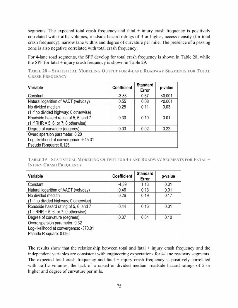
75

segments. The expected total crash frequency and fatal + injury crash frequency is positively correlated with traffic volumes, roadside hazard ratings of 3 or higher, access density (for total crash frequency), narrow lane widths and degree of curvature per mile. The presence of a passing zone is also negative correlated with total crash frequency.

For 4-lane road segments, the SPF develop for total crash frequency is shown in Table 28, while the SPF for fatal + injury crash frequency is shown in Table 29.

TABLE 28 – STATISTICAL MODELING OUTPUT FOR 4-LANE ROADWAY SEGMENTS FOR TOTAL CRASH FREQUENCY


Constant -3.83 0.67 <0.001 Natural logarithm of AADT (veh/day) 0.55 0.08 <0.001 No divided median (1 if no divided highway; 0 otherwise)

0.25 0.11 0.03


0.30 0.10 0.01

Degree of curvature (degrees) 0.03 0.02 0.22 Overdispersion parameter: 0.20 Log-likelihood at convergence: -645.31 Pseudo R-square: 0.126

TABLE 29 – STATISTICAL MODELING OUTPUT FOR 4-LANE ROADWAY SEGMENTS FOR FATAL + INJURY CRASH FREQUENCY


Constant -4.39 1.13 0.01 Natural logarithm of AADT (veh/day) 0.46 0.13 0.01 No divided median (1 if no divided highway; 0 otherwise)

0.26 0.19 0.17


0.44 0.16 0.01

Degree of curvature (degrees) 0.07 0.04 0.10 Overdispersion parameter: 0.32 Log-likelihood at convergence: -370.01 Pseudo R-square: 0.090

The results show that the relationship between total and fatal + injury crash frequency and the independent variables are consistent with engineering expectations for 4-lane roadway segments. The expected total crash frequency and fatal + injury crash frequency is positively correlated with traffic volumes, the lack of a raised or divided median, roadside hazard ratings of 5 or higher and degree of curvature per mile.

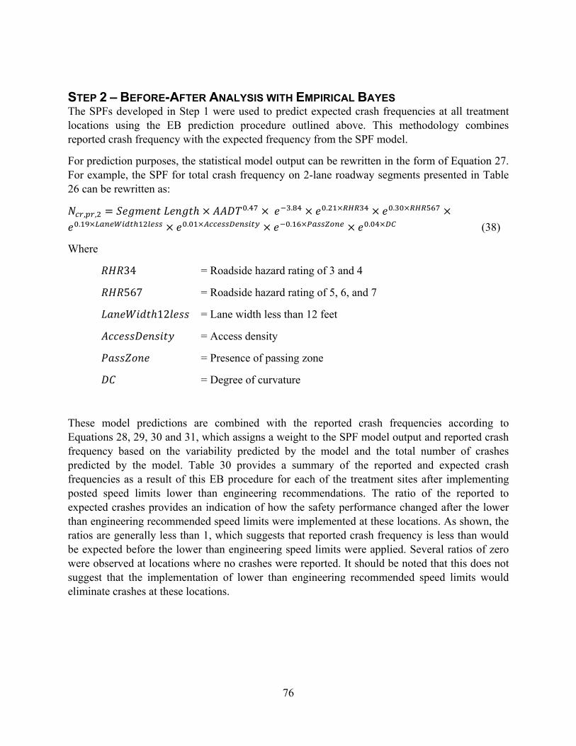
76

STEP 2 – BEFORE-AFTER ANALYSIS WITH EMPIRICAL BAYES The SPFs developed in Step 1 were used to predict expected crash frequencies at all treatment locations using the EB prediction procedure outlined above. This methodology combines reported crash frequency with the expected frequency from the SPF model.

For prediction purposes, the statistical model output can be rewritten in the form of Equation 27. For example, the SPF for total crash frequency on 2-lane roadway segments presented in Table 26 can be rewritten as:

, , . . . .

. . . . (38)

Where

34 = Roadside hazard rating of 3 and 4

567 = Roadside hazard rating of 5, 6, and 7

12 = Lane width less than 12 feet

= Access density

= Presence of passing zone

= Degree of curvature

These model predictions are combined with the reported crash frequencies according to Equations 28, 29, 30 and 31, which assigns a weight to the SPF model output and reported crash frequency based on the variability predicted by the model and the total number of crashes predicted by the model. Table 30 provides a summary of the reported and expected crash frequencies as a result of this EB procedure for each of the treatment sites after implementing posted speed limits lower than engineering recommendations. The ratio of the reported to expected crashes provides an indication of how the safety performance changed after the lower than engineering recommended speed limits were implemented at these locations. As shown, the ratios are generally less than 1, which suggests that reported crash frequency is less than would be expected before the lower than engineering speed limits were applied. Several ratios of zero were observed at locations where no crashes were reported. It should be noted that this does not suggest that the implementation of lower than engineering recommended speed limits would eliminate crashes at these locations.

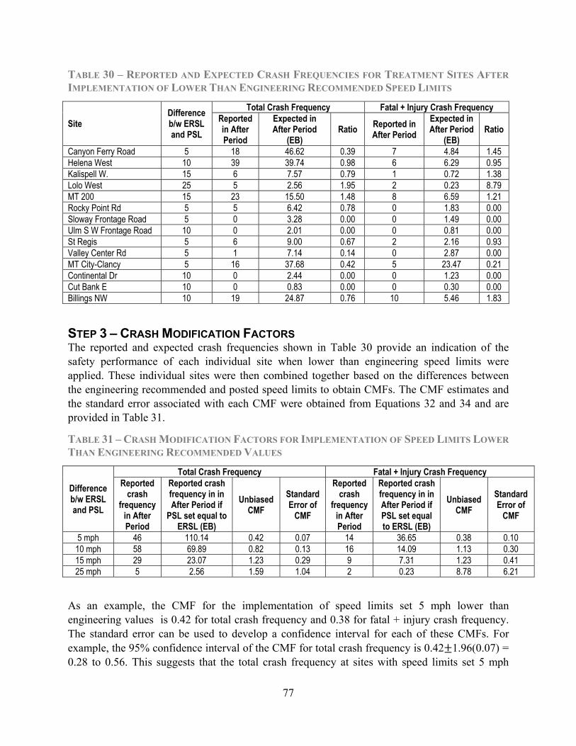
77

TABLE 30 – REPORTED AND EXPECTED CRASH FREQUENCIES FOR TREATMENT SITES AFTER IMPLEMENTATION OF LOWER THAN ENGINEERING RECOMMENDED SPEED LIMITS

Site Difference b/w ERSL and PSL

Total Crash Frequency Fatal + Injury Crash Frequency Reported in After Period

Expected in After Period

(EB) Ratio Reported in

After Period Expected in After Period

(EB) Ratio

Canyon Ferry Road 5 18 46.62 0.39 7 4.84 1.45 Helena West 10 39 39.74 0.98 6 6.29 0.95 Kalispell W. 15 6 7.57 0.79 1 0.72 1.38 Lolo West 25 5 2.56 1.95 2 0.23 8.79 MT 200 15 23 15.50 1.48 8 6.59 1.21 Rocky Point Rd 5 5 6.42 0.78 0 1.83 0.00 Sloway Frontage Road 5 0 3.28 0.00 0 1.49 0.00 Ulm S W Frontage Road 10 0 2.01 0.00 0 0.81 0.00 St Regis 5 6 9.00 0.67 2 2.16 0.93 Valley Center Rd 5 1 7.14 0.14 0 2.87 0.00 MT City-Clancy 5 16 37.68 0.42 5 23.47 0.21 Continental Dr 10 0 2.44 0.00 0 1.23 0.00 Cut Bank E 10 0 0.83 0.00 0 0.30 0.00 Billings NW 10 19 24.87 0.76 10 5.46 1.83

STEP 3 – CRASH MODIFICATION FACTORS The reported and expected crash frequencies shown in Table 30 provide an indication of the safety performance of each individual site when lower than engineering speed limits were applied. These individual sites were then combined together based on the differences between the engineering recommended and posted speed limits to obtain CMFs. The CMF estimates and the standard error associated with each CMF were obtained from Equations 32 and 34 and are provided in Table 31.

TABLE 31 – CRASH MODIFICATION FACTORS FOR IMPLEMENTATION OF SPEED LIMITS LOWER THAN ENGINEERING RECOMMENDED VALUES

Difference b/w ERSL and PSL

Total Crash Frequency Fatal + Injury Crash Frequency Reported

crash frequency

in After Period

Reported crash frequency in in After Period if

PSL set equal to ERSL (EB)

Unbiased CMF

Standard Error of

CMF

Reported crash

frequency in After Period

Reported crash frequency in in After Period if PSL set equal to ERSL (EB)

Unbiased CMF

Standard Error of

CMF

5 mph 46 110.14 0.42 0.07 14 36.65 0.38 0.10 10 mph 58 69.89 0.82 0.13 16 14.09 1.13 0.30 15 mph 29 23.07 1.23 0.29 9 7.31 1.23 0.41 25 mph 5 2.56 1.59 1.04 2 0.23 8.78 6.21

As an example, the CMF for the implementation of speed limits set 5 mph lower than engineering values is 0.42 for total crash frequency and 0.38 for fatal + injury crash frequency. The standard error can be used to develop a confidence interval for each of these CMFs. For example, the 95% confidence interval of the CMF for total crash frequency is 0.42 1.96(0.07) = 0.28 to 0.56. This suggests that the total crash frequency at sites with speed limits set 5 mph

78

lower than engineering recommendations is expected to be 0.28 to 0.56 times the crash frequency expected if the speed limit was set in accordance with engineering recommendations. Since 1.0 is not within the confidence interval, the effect is statistically significant. The 95% confidence interval for the CMF for fatal + injury crash frequency is 0.18 to 0.58, which also suggests a statistically significant reduction in fatal + injury crash frequency when setting posted speed limits 5 mph lower than engineering recommendations.

Table 31 reveals that the CMF increases with the difference between the engineering recommended and posted speed limits. The CMFs suggest that setting speed limits only 5 mph below the engineering recommended value is associated with a statistically significant reduction in total and fatal + injury crash frequency. Setting speed limits 10 mph below the engineering recommended value is associated with a reduction in total crash frequency and an increase in fatal + injury crash frequency; however, neither of these changes is statistically significant as the confidence interval for both CMFs includes 1.0. Setting speed limits 15 mph or more below the engineering recommended value is associated with an increase in total and fatal + injury crash frequency; however, again, neither of these estimates is statistically significant.

79

CONCLUSIONS AND RECOMMENDATIONS FOR IMPLEMENTATION This study considered the safety and operational effects of setting speed limits lower than engineering recommendations in the state of Montana. A survey of state transportation agencies found that this a common practice among responding agencies. Among the responding agencies who have established posted speed limits lower than engineering recommendations, the maximum difference between the posted speed limit and the engineering recommended speed limit was 10 mph. A citywide reduction in the posted speed limit in Idaho found that operating speed reductions were not commensurate with the posted speed limit reduction, and that the difference between the 85th-percentile operating speed and posted speed limit increased (operating speeds were higher than the posted speed limit) after the speed limits were reduced. New York State will allow local transportation agencies to post speed limits that are consistent with 67th-percentile operating speeds.

The operating speed evaluation conducted in the present study produced results that were consistent with other state transportation agency experiences when setting posted speed limits lower than engineering recommendations. When the posted speed limit was set only 5 mph lower than the engineering posted speed limit, drivers tend to more closely comply with the posted speed limit. Compliance tends to lessen as the difference between the engineering recommended posted speed limit and the posted speed limit increases. When the posted speed limit is set 15 to 25 mph lower than the engineering recommended speed, there appears to be a low level of compliance with the posted speed limit. The practice of light enforcement, which was defined as highway patrol vehicles making frequent passes through locations with posted speed limits set lower than engineering recommendations, appeared to have only a nominal effect on vehicle operating speeds. Known heavy enforcement, defined as a stationary highway patrol vehicle present within the speed zone, reduced mean and 85th-percentile vehicle operating speeds by approximately 4 mph. Additionally, known heavy enforcement increased the odds that drivers would comply with the posted speed limit.

The safety evaluation included 6 sites with posted speed limits set 5 mph lower than engineering recommendations; 5 sites with posted speed limits set 10 mph lower than engineering recommendations; 2 sites with posted speed limits set 15 mph lower than engineering recommendations; and one site with a posted speed limit set 25 mph lower than engineering recommendations. While this is a small number of sites, the before-after analysis found that there is a statistically significant reduction in total and fatal + injury crashes at locations with posted speed limits set 5 mph lower than engineering recommendations. Locations with posted speed limits set 10 mph lower than engineering recommendations experienced a decrease in total crash frequency but an increase in fatal + injury crash frequency. The safety effects of setting speed limits 15 to 25 mph lower than engineering recommendations is less clear as the results were not statistically significant, likely due to the small sample of sites included in the evaluation.

When considering other state transportation agency practices, and the speed and safety evaluation results from the present study, it appears that setting posted speed limits 5 mph lower than the engineering recommended practice may produce total and fatal + injury crash benefits,

80

presumably because drivers appear to more closely comply with the speed limits in these locations. While known heavy enforcement was found to reduce mean and 85th-percentile operating speeds while the patrol vehicles were positioned within the speed zone, this effect likely diminishes when the enforcement period concludes. The practice of setting posted speed limits 15 or 25 mph lower than engineering recommended speed limits does not appear to produce operating speeds consistent with the posted speed limit. While the sample size is small, there is preliminary evidence to suggest that setting speed limits 15 or 25 mph below the engineering recommended level may not offer safety benefits.

As noted above, a limitation of the present study was few sites that had posted speed limits set 15 or 25 mph below engineering recommended levels. If Montana is to continue this practice, and plans to post speed limits that are 15 or 25 mph below engineering recommendations, the speed and safety evaluations conducted as part of this study should be expanded to include the additional locations. More sites will afford an opportunity to include more site-years of data in an observational before-after safety study so that the confidence level associated with the CMF is narrowed. Further, this practice will offer additional sites to assess the value of known heavy enforcement programs. Finally, the small number of sites that currently implement posted speed limits lower than engineering recommendations in Montana made it difficult to identify statistically significant changes in the crash type distribution as a result of this practice. If this practice is implemented at additional sites, future research should seek to identify if statistically significantly changes to the crash type distribution are observed.

81

PRACTICAL APPLICATION OF FINDINGS Based on the findings from the present study, the practice of setting speed limits lower than engineering-recommended values appears to be most prudent when the difference is 5 mph. Among the 5, 10, 15, and 25 mph differences evaluated, driver compliance is greatest when the speed limit is set 5 mph lower than the engineering-recommended value. Similarly, safety benefits were associated with this practice when considering both total and fatal + injury crashes. Driver speed compliance appears to diminish as the magnitude of the difference between the posted speed limit and engineering-recommended speed limit increases. There does appear to be a reduction in total crashes when the posted speed limit is set 10 mph below the engineering-recommended speed limit, but this is offset by an expected increase in fatal + injury crashes associated with this practice. Setting posted speed limits 15 or 25 mph below the engineering-recommended speed limit produces a low level of driver speed compliance, and the sample of sites included in this study found safety disbenefits associated with this practice.

82

REFERENCES

AASHTO (American Association of State Highway Transportation Officials). Highway Safety Manual 1st Edition. (2010).

AASHTO (American Association of State Highway Transportation Officials). A Policy on the Geometric Design of Highways and Streets. (2011).

AASHTO (American Association of State Highway Transportation Officials), “AASHTO Subcommittee on Traffic Engineering.” (2014) http://scote.transportation.org/Pages/Members.aspx.

Abdel-Aty, M. and Pande, A., “Identifying Crash Propensity Using Specific Traffic Speed Conditions.” Journal of Safety Research, Vol. 36 (2005) pp. 97-108.

Acqua, G. D. and Russo, F., “Safety Performance Functions for Low-Volume Roads.” Proceedings, 90th Annual Meeting of the Transportation Research Board, Washington, D.C. (2011).

Ahlin, F. J. “An Investigation in the Consistency of Driver’s Speed Choice.” Doctoral Dissertation, University of Toronto, Toronto, ON. (1979).

Aljanahi, A. A. M., Rhodes, A. H., and Metcalde, A. V., “Speed, Speed Limits and Road Traffic Accidents under Free Flow Conditions.” Accident Analysis & Prevention, Vol. 31, Nos. 1-2 (1999) pp. 161-168.

Benekohal, R. F. and Wang, L., “Relationship between Initial Speed and Speed inside a Highway Work Zone.” Transportation Research Record: Journal of the Transportation Research Board, No. 1441 (1994) pp. 41-48.

Bham, G. H., Long, S., Baik, H., Ryan, T., Gentry, L., Lall, K., Arezoumandi, M., Liu, D., Li, T., and Schaeffer, B., “Evaluation of Variable Speed Limits on I-270/I-255 in St. Louis”. TRyy0825, RI 08‐025, Missouri Department of Transportation, Rolla, MO (2010) pp. 1-39.

Caltrans, “2014 California Manual for Setting Speed Limits.” California Department of Transportation (2014) pp. 1-91.

Cameron, M. H., Newstead, S., Diamantopoulou, K., and Oxley, P., “The Interaction between Speed Camera Enforcement and Speed-Related Mass Media Publicity in Victoria.” Proceedings, 47th Annual Proceedings of the Association for the Advancement of Automotive Medicine, Lisbon, Portugal (2003) pp. 267-282.

Chen, H., Zhang, Y., Wang, Z., and Lu, J., “Identifying Crash Distributions and Prone Locations by Lane Groups at Freeway Diverging Areas.” Accident Analysis & Prevention, Vol. 32, No. 2 (2002) pp. 129-138.

83

Cirillo, J. A. “Interstate System Accident Research Study II, Interim Report II.” Public Roads, Vol. 35, No. 3 (1968) pp. 71-75.

Cruzado, I. and Donnell, E. T., “Evaluating Effectiveness of Dynamic Speed Display Signs in Transition Zones of Two-Lane Rural Highways in Pennsylvania.” Transportation Research Record: Journal of the Transportation Research Board, No. 2112 (2009) pp. 1-8.

Cruzado, I. and Donnell, E. T., “Factors Affecting Driver Speed Choice along Two-Lane Rural Highway Transition Zones.” Journal of Transportation Engineering, Vol. 136, No. 8 (2010) pp. 755-764.

Davis, G. A., “Is the Claim that ‘Variance Kills’ an Ecological Fallacy?” Accident Analysis & Prevention, Vol. 32, No. 3 (2002) pp. 343-346.

De Pelsmacker, P., and Janssens, W., “The Effect of Norms, Attitudes and Habits on Speeding Behavior: scale Development and Model Building Estimation.” Accident Analysis & Prevention, Vol. 39, No. 1 (2007) pp. 6-15.

Debnath, A. K., Blackman, R., and Haworth, N. “A Tobit Model for Analyzing Speed Limit Compliance in Work Zones.” Safety Science, Vol. 70 (2014) pp. 367-377.

Dimaiuta, M., Donnell, E. T., Himes, S. C., and Porter, R. J., “Speed Models in North America.” TRB E-Circular 151 – Modeling Operating Speed: Synthesis Report, Washington, D.C., Transportation Research Board, National Research Council (2011) pp. 3-42.

Dixon, K. K., Wu, C. H., Sarasua, W., and Daniels, J., “Posted and Free-Flow Speeds for Rural Multilane Highways in Georgia.” Journal of Transportation Engineering, Vol. 125, No. 6 (1999) pp. 487-494.

Donnell, E. T., Himes, S. C., Mahoney, K. M., Porter, R. J., and McGee, H., “Speed Concepts: Informational Guide.” FHWA-SA-10-001, Federal Highway Administration, U.S. Department of Transportation, Washington, D.C. (2009) pp. 1-50.

Donnell, E. T., Ni, Y., Adolini, M., Elefteriadou, L., “Speed Prediction Models for Trucks on Two-Lane Rural Highways.” Transportation Research Record: Journal of the Transportation Research Board, No. 1751, (2001) pp. 44-55.

Elliot, M. A., Armitage, C. J., Baughan, C. J., “Drivers’ Compliance with Speed Limits: An Application of the Theory of Planned Behavior.” The Journal of Applied Psychology, Vol. 88, No. 5 (2003) pp. 964-972.

Elvik, R., “Speed and Road Safety: Synthesis of Evidence from Evaluation Studies.” Transportation Research Record: Journal of the Transportation Research Board, No. 1908, (2005) pp. 59-69.

Elvik, R., Christensen, P., Amundsen, A., “Speed and Road Accidents: An Evaluation of the Power Model.” TØI report 740, Transportokonomisk Institutt, Oslo, Norway (2004) pp. 1-134.

84

Elvik, R., Hoye, A., Vaa, T., and Sorensen, M., The Handbook of Road Safety Measures. Emerald Group Publishing Limited, Bingley, U.K., 2nd Edition (2009), pp. 1-1124.

Farmer, C. M. “Relationship of Traffic Fatality Rates to Maximum State Speed Limits.” Insurance Institute for Highway Safety, Arlington, VA, April 2016.

FDOT (Florida Department of Transportation), “Speed Zoning for Highways, Roads and Streets in Florida.” Topic No. 750-010-002, Traffic Engineering & Operations Office, Florida Department of Transportation, Tallahassee, FL (2010) pp. 1.1-16.6.

FHWA (Federal Highway Administration), USLIMITS2: A Web-Based Tool for Setting Appropriate Speed Limits. Washington, D.C.: Federal Highway Administration, U.S. Department of Transportation, (2014a). Informational flyer. http://safety.fhwa.dot.gov/uslimits/documents/uslimits2_flyer_lowres121012.pdf

FHWA (Federal Highway Administration), “CMF Clearinghouse.” (2014b) hhtp://www.cmfclearinghouse.org/index.cfm. Accessed: 10/1/2014

Figueroa, A. and Tarko, A., “Reconciling Speed Limits with Design Speeds.” FHWA/IN/JTRP-2004/26, Purdue University, West Lafayette, Ind. (2004) pp. 1-165.

Fitzpatrick, K., Carlson, P., Brewer, M. A., Wooldridge, M. D., and Miaou, S., “Design Speed, Operating Speed, and Posted Speed Practices.” NCHRP Report 504, Transportation Research Board, National Research Council, Washington, D.C. (2003) pp. 1-92.

Fitzpatrick, K., Elefteriadou, L., Harwood, D. W., Collins, J., McFadden, J., Anderson, I. B., Krammes, R. A., Irizarry, N., Parma, K., Bauer, K. M., Passetti, K., “Speed Prediction Models for Two-Lane Rural Highways.” Report FHWA-RD-99-171, Federal Highway Administration, U.S. Department of Transportation, Washington, D.C. (2000) pp. 1-213.

Forbes, G. J., Gardner, T., McGee, H., and Srinivasan, R., “Methods and Practices for Setting Speed Limits.” FHWA-SA-12-004, Federal Highway Administration, U.S. Department of Transportation, Washington, D.C. (2012) pp. 1-109.

Friedman, L. S., Hedeker, D., and Richter, E. D., “Long-Term Effects of Repealing the National Maximum Speed Limit in the United States.” American Journal of Public Health, Vol. 99, No. 9 (2009) pp. 1626-1631.

Gong, H. and Stamatiadis, N., “Operating Speed Prediction Models for Horizontal Curves on Rural Four-Lane Highways.” Proceedings of the 87th Annual Meeting of the Transportation Research Board, Washington, D.C., (2008).

Google. “Google Earth”. (2015).

Gross, F., Persaud, B., Lyon, C., “A Guide to Developing Quality Crash Modification Factors.” FHWA-SA-10-032, Federal Highway Administration, U.S. Department of Transportation, Washington, D.C. (2010) pp. 1-64.

85

Haglund, M. and Aberg, L., “Speed Choice in Relation to Speed Limit and Influences from Other Drivers.” Transportation Research Part F: Traffic Psychology and Behavior 3 (2000) pp. 39-51.

Hauer, E. Observational Before-After Studies in Road Safety: Estimating the Effect of Highway and Traffic Engineering Measures in Road Safety. Emerald Group Publishing Limited, Bingley, UK (1997).

Hauer, E., “Speed and Safety.” Transportation Research Record: Journal of the Transportation Research Board, No. 2103 (2009) pp. 10-17.

Hauer, E., Ahlin, F. J., and Bowser, J. S., “Speed Enforcement and Speed Choice.” Accident Analysis & Prevention, Vol. 14, No. 4 (1981) pp. 267-278.

Himes, S. C., Donnell, E. T., and Porter, R. J., “Posted Speed Limit: To Include or Not to Include in Operating Speed Models.” Transportation Research Part A: Policy and Practice, Vol. 52 (2013) pp. 23-33.

Institute of Transportation Engineers, Manual of Transportation Engineering Studies. Prentice Hall, Englewood (2010) 2nd Edition pp. 1-514

Islam, M. N. and Seneviratne, P. N., “Evaluation of Design Consistency of Two-Lane Rural Highways.” ITE Journal, Vol. 64, No. 2 (1994) pp. 28-31.

Jaarsma, R., Louwerse, R., Dijkstra, A., and de Vries, J., “Making Minor Rural Road Networks Safer: The Effects of 60 km/h-Zones.” Accident Analysis & Prevention, Vol. 43, No. 4 (2011) pp. 1508-1515.

Jessen D. R., Schurr, K. S., McCoy, P.T., Pesti, G., and Huff, R. R., “Operating Speed Prediction on Crest Vertical Curves of Rural Two-Lane Highways in Nebraska.” Transportation Research Record: Journal of the Transportation Research Board, No. 1751 (2001) pp. 67-75.

Kockelman, K., Bottom, J., Kweon, Y.J., Ma, J. and Wang, X. “Safety Impacts and Other Implications of Raised Speed Limits on High-Speed Roads.” NCHRP Web-Only Document 90, Project 17-23. (2006).

Krammes, R. A., Brackett, R. Q., Shafer, M. A., Ottesen, J. L., Anderson, I. B., Fink, K. L., Collins, K. M., Pendleton, O. J., and Messer, C. J., “Horizontal Alignment Design Consistency for Rural Two-Lane Highways.” FHWA-RD-94-034, Federal Highway Administration, U.S. Department of Transportation, Washington, D.C. (1995) pp. 1-127.

Ksaibati, K. and Evans, B., “WRRSP: Wyoming Rural Road Safety Program.” FHWA-WY-09/06F, Wyoming Department of Transportation, Federal Highway Administration, U.S. Department of Transportation, Washington, D.C. (2009) pp.1-272.

Lee, C. and Li, X., “Analysis of Injury Severity of Drivers Involved in Single- and Two-Vehicle Crashes on Highways in Ontario.” Accident Analysis & Prevention, Vol. 71, October (2014) pp. 286-295.

86

Mahoney, K. M., Porter, R. J., Donnell, E. T., Lee, D., and Pietrucha, M. T., “Evaluation of Centerline Rumble Strips on Lateral Vehicle Placement and Speed on Two-Lane Highways.” FHWA-PA-2002-034-97-04, Pennsylvania Transportation Institute, Penn State University, University Park, PA (2003).

Mahoney, K. M., Porter, R. J., Taylor, D. R., and Kulakowski, B. R., “Design of Construction Work Zones.” NCHRP Report 581, Transportation Research Board, National Research Council, Washington, D.C. (2007) pp. 1-65.

Maryland Department of Transportation, “Speed Limits.” (2014) http://www.sha.maryland.gov/Index.aspx?PageId=295. Accessed: 10/1/2014.

McFadden, J. and Elefteriadou, L., “Evaluating Horizontal Alignment Design Consistency of Two-Lane Rural Highways.” Transportation Research Record: Journal of the Transportation Research Board, No. 1737 (2000) pp. 9-16.

McFadden, J., Yang, W. T., and Durrans, S. R., “Application of Artificial Networks to Predict Speeds on Two-Lane Rural Highways.” Transportation Research Record: Journal of the Transportation Research Board, No. 1751 (2001) pp. 9-17.

Meier, K. J. and Morgan, D. R., “Citizen Compliance with Public Policy: The National Maximum Speed Law.” The Western Political Quarterly, Vol. 35, No. 2 (1982) pp. 258-273.

Misaghi, P. and Hassan, Y., “Modeling Operating Speed and Speed Differential on Two-Lane Rural Roads.” Journal of Transportation Engineering, Vol. 131, No. 6 (2005) pp. 408-417.

Newstead, S. and Cameron, M. H., “Evaluation of the Crash Effects of the Queensland Speed Camera Program.” Report 204, Monash University Accident Research Centre, Victoria, Australia (2003) pp. 1-35.

Nilsson, G., “An Investigation in the Consistency of Driver’s Speed Choice.” Doctoral Dissertation, Lund Institute of Technology, Lund, Sweden (2004).

ODOT (Ohio Department of Transportation), “Speed Zones – Ohio Speed Limits.” (2014) http://www.dot.state.oh.us/districts/D01/PlanningPrograms/trafficstudies/SpeedZoens/Pages/default.aspx Accessed: 10/1/2014

Park, E. S., Park, J., and Lomax, T. J., “A Fully Bayesian Multivariate Approach to Before-After Safety Evaluation.” Accident Analysis & Prevention, Vol. 42, No. 4 (2010) pp. 1118-1127.

Parker, M. R., “Effects of Raising and Lowering Speed Limits on Selected Roadway Sections.” FHWA-RD-92-084, Federal Highway Administration, U.S. Department of Transportation, Washington, D.C. (1997) pp. 1-166.

87

Peltola, H., “Seasonally Changing Speed Limits Effects on Speeds and Accidents.” Transportation Research Record: Journal of the Transportation Research Board, No. 1734 (2000) pp. 46-51.

Persaud, B., and Lyon, C., “Empirical Bayes Before-After Studies: Lessons Learned from Two Decades of Experience and Future Directions.” Accident Analysis & Prevention, Vol. 39 (2007) pp. 546-555.

Poe, C. M., Tarris, J. P., and Mason Jr., J. M., “Operating Speed Approach to Geometric Design of Low-Speed Urban Streets.” PTI Report 9606, Pennsylvania Transportation Institute, Penn State University, University Park, PA (1996a) pp. 10.1-10.9.

Poe, C.M., J.P. Tarris and J.M. Mason, Jr. “Relationship of operating speeds to roadway geometric design speeds.” FHWA-RD-96-024. Pennsylvania Transportation Institute, University Park, PA (1996b).

Polus, A., Fitzpatrick, K., and Fambro, D. B., “Predicting Operating Speeds on Tangent Sections of Two-Lane Rural Highways.” Transportation Research Record: Journal of the Transportation Research Board, No. 1737 (2000) pp.50-57.

Qualtrics, “Qualtrics.” (2014) http://www.qualtrics.com/.

Quimby, A., Maycock, G., Palmer, C., and Buttress, S., “The Factors That Influence a Driver’s Choice of Speed – A Questionnaire Study.” TRL Report 325, Transport Research Laboratory, U.K. (1999) pp. 1-34.

Rämä, P., “Effects of Weather-Controlled Variable Message Signing on Driver Behaviour.” Doctoral Dissertation, VTT Technical Research Centre of Finland, Helsinki University of Technology, Helsinki, Finland (2004) pp.1-55.

Renski, H., Khattak, A. J., Council, F. M., “Effects of Speed Limit Increases on Crash Injury Severity: Analysis of Single-Vehicle Crashes on North Carolina Interstate Highways.” Transportation Research Record: Journal of the Transportation Research, No. 1665 (1999) pp. 100-108.

Retting, R. A. and Farmer, C. M., “Evaluation of Speed Camera Enforcement in the District of Columbia.” Transportation Research Record: Journal of the Transportation Research Board, No. 1830 (2003) pp. 34-37.

Shinar, D. and Stiebel, J., “The Effectiveness of Stationary versus Moving Police Vehicles on Compliance with Speed Limit.” Human Factors: The Journal of the Human Factors and Ergonomics Society, Vol. 28, No. 3 (1986) pp. 365-371.

Shinar, D., Traffic Safety and Human Behavior. Emerald Group Publishing Limited, Bingley, U.K. (2007) 2nd Edition pp. 1-776.

Snedecor, G. W., and Cochran, W. G., Statistical Methods, Iowa State University Press, Ames, IA, 8th Edition. (1989).

88

Solomon, D., Accidents on Main Rural Highways Related to Speed, Driver, and Vehicle. US Department of Commerce, Federal Bureau of Highways, Washington DC. (1964)

State of Minnesota, “2013 Minnesota Statutes.” The Office of the Revisor of Statutes. (2013) http://www.revisor.mn.gov/statutes/?id=169.14 Accessed: 10/1/2014.

Torbic, D. J., Gilmore, D. K., Bauer, K. M., Bokenroger, C. D., Harwood, D. W., Lucas, L. M., Frazier, R. J., Kinzel, C. S., Petree, D. L., and Forsberg, M. D., “Design Guidance for High-Speed to Low-Speed Transition Zones for Rural Highways.” NCHRP Report 737, Transportation Research Board, National Research Council, Washington, D.C. (2012) pp. 1-88.

Transportation Research Board, Managing Speed: Review of Current Practice for Setting and Enforcing Speed Limits. Transportation Research Board, National Research Council, Washington, D.C. (1998) pp. 1-427.

Transportation Research Board, Highway Capacity Manual 2010. Transportation Research Board, National Research Council, Washington, D.C. (2010).

TXDOT (Texas Department of Transportation), “Procedures for Establishing Speed Zones.” Texas Department of Transportation (2012) pp. 1.1-5.24.

Vaa, T., “Increased Police Enforcement: Effects on Speed.” Accident Analysis & Prevention, Vol. 29, No. 3 (1997) pp. 373-385.

Voigt, A. P. and Krammes, R. A., “An Operational and Safety Evaluation of Alternative Horizontal Curve Design Approaches on Rural Two-Lane Highways.” Transportation Research Circular, E-C003, No. 11 (1998) pp. 1-8.

Wang, C., Dixon, K. K., and Jared, D., “Evaluation of Speed Reduction Strategies.” Transportation Research Record: Journal of the Transportation Research Board, No. 1824 (2003) pp. 44-53.

Wang, Z. B., Cao, B., Deng, W., Lu, J., and Zhang, Z., “Safety Evaluation of Truck-Related Crashes at Freeway Diverge Areas.” Proceedings, 90th Annual Meeting of the Transportation Research Board, Washington, D.C. (2011).

Warren, D., Xu, G., and Srinivasan, R., “Setting Speed Limits for Safety.” Public Roads, Vol. 77, No. 2 (2013).

Wei, L. and Tarko, A., “Safety Effect of Arterial Signal Coordination.” Proceedings, 90th Annual Meeting of the Transportation Research Board, Washington, D.C. (2011).

WHO (World Health Organization), “World Report on Road Traffic Injury Prevention.” World Health Organization, Geneva, Switzerland (2004).

WSDOT (Washington State Department of Transportation), “Speed Limits.” Washington State Department of Transportation (2014). http://www.wsdot.wa.gov/Operations/Traffic/speedlimits.htm Accessed: 10/1/2014.

A - 1

APPENDIX A: STATE TRANSPORTATION AGENCY SURVEY

A - 2

Default Question Block

Instructions:

As part of a Montana Department of Transportation (MDT) study titled "Speed Limits Set Lower than Engineering Recommendations," our research team is interested in your feedback to a short survey. The survey will help us to meet the project objectives, which are to:

Quantify mean vehicle speeds and the level of compliance with posted speed limits that are below engineering recommendations under various levels of law enforcement presence.

Determine the minimum level of enforcement necessary to achieve a specific target posted speed limit compliance rate.

Quantify the impacts of lower-than-engineering recommended posted speed limits on traffic safety, measured by the frequency and severity of crashes.

Identify other potential safety or operational impacts of lower-than-engineering recommended posted speed limits.

The survey is organized into two parts based on the objectives listed above. The survey should take approximately 5 minutes to complete. Thank you for your time and thoughtful consideration.

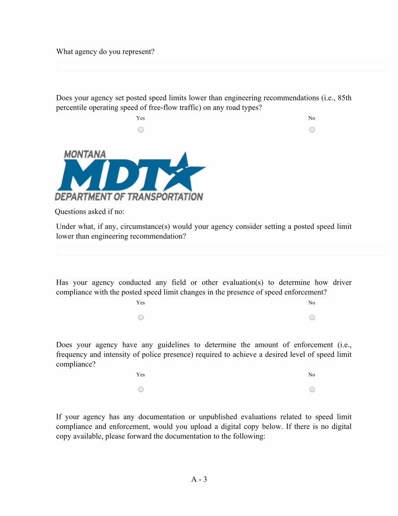
A - 3

What agency do you represent?

Does your agency set posted speed limits lower than engineering recommendations (i.e., 85th percentile operating speed of free-flow traffic) on any road types?

Yes No

Questions asked if no:

Under what, if any, circumstance(s) would your agency consider setting a posted speed limit lower than engineering recommendation?

Has your agency conducted any field or other evaluation(s) to determine how driver compliance with the posted speed limit changes in the presence of speed enforcement?

Yes No

Does your agency have any guidelines to determine the amount of enforcement (i.e., frequency and intensity of police presence) required to achieve a desired level of speed limit compliance?

Yes No

If your agency has any documentation or unpublished evaluations related to speed limit compliance and enforcement, would you upload a digital copy below. If there is no digital copy available, please forward the documentation to the following:

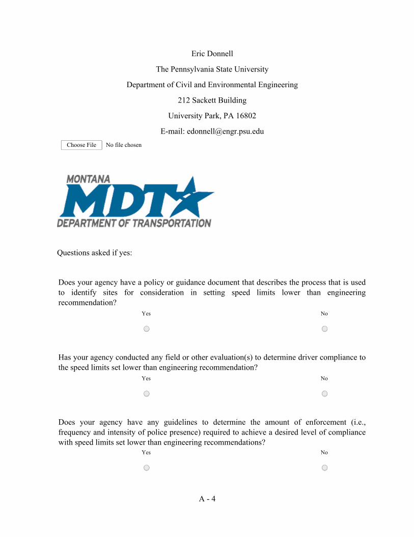
A - 4

Eric Donnell

The Pennsylvania State University

Department of Civil and Environmental Engineering

212 Sackett Building

University Park, PA 16802

E-mail: [email protected] Choose File No file chosen

Questions asked if yes:

Does your agency have a policy or guidance document that describes the process that is used to identify sites for consideration in setting speed limits lower than engineering recommendation?

Yes No

Has your agency conducted any field or other evaluation(s) to determine driver compliance to the speed limits set lower than engineering recommendation?

Yes No

Does your agency have any guidelines to determine the amount of enforcement (i.e., frequency and intensity of police presence) required to achieve a desired level of compliance with speed limits set lower than engineering recommendations?

Yes No

A - 5

Has your agency conducted any field or other evaluation(s) to determine the safety effects of roads that have speed limits set lower than engineering recommendations?

Yes No

Has your agency noticed any other issues with respect to speed limits set lower than engineering recommendations on your roadways?

If your agency has a policy, guidance documentation, or any unpublished evaluations of roads that contain posted speed limits set lower than engineering recommendation, please upload a digital copy below. If a digital copy is unavailable, please forward a paper copy to the following:

Eric Donnell

The Pennsylvania State University

Department of Civil and Environmental Engineering

212 Sackett Building

University Park, PA 16802

E-mail: [email protected] Choose File No file chosen

B - 1

APPENDIX B: SCHEMATIC DRAWINGS OF SPEED DETECTOR

LOCATIONS

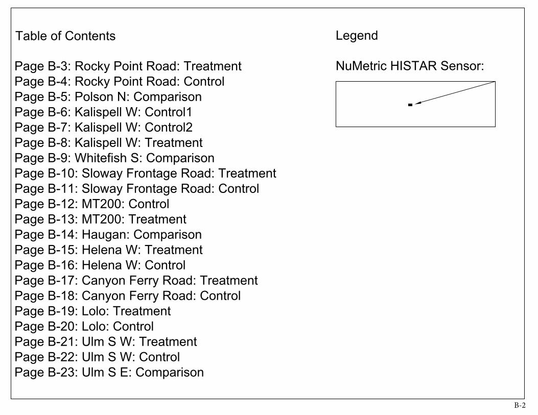
Legend

NuMetric HISTAR Sensor:

Table of Contents

Page B-3: Rocky Point Road: TreatmentPage B-4: Rocky Point Road: ControlPage B-5: Polson N: ComparisonPage B-6: Kalispell W: Control1Page B-7: Kalispell W: Control2Page B-8: Kalispell W: TreatmentPage B-9: Whitefish S: ComparisonPage B-10: Sloway Frontage Road: Treatment Page B-11: Sloway Frontage Road: Control Page B-12: MT200: ControlPage B-13: MT200: TreatmentPage B-14: Haugan: ComparisonPage B-15: Helena W: TreatmentPage B-16: Helena W: ControlPage B-17: Canyon Ferry Road: Treatment Page B-18: Canyon Ferry Road: Control Page B-19: Lolo: TreatmentPage B-20: Lolo: ControlPage B-21: Ulm S W: TreatmentPage B-22: Ulm S W: ControlPage B-23: Ulm S E: Comparison

B-2

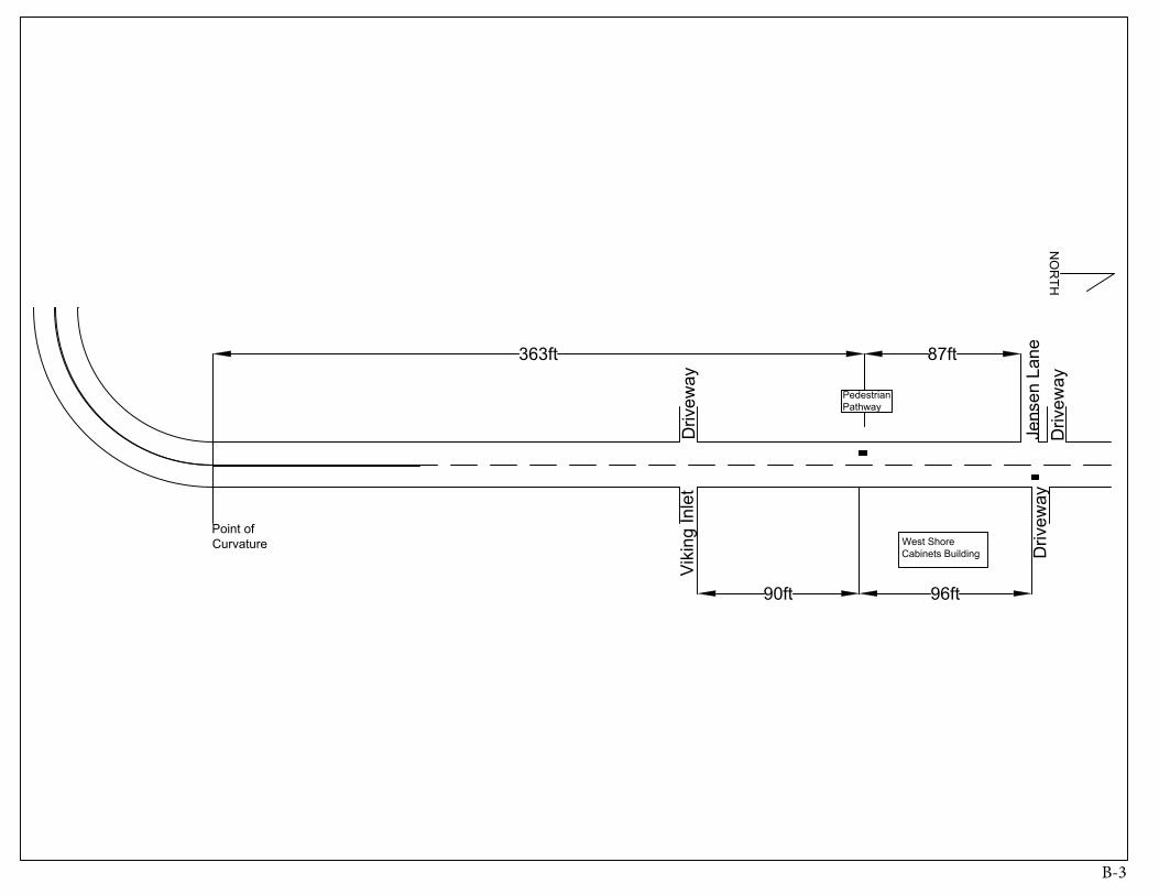
West ShoreCabinets Building

PedestrianPathway

Vik

ing

Inle

t

Jens

en L

ane

Driv

eway

Driv

eway

Driv

eway

Point ofCurvature

363ft 87ft

90ft 96ft

NO

RTH

B-3

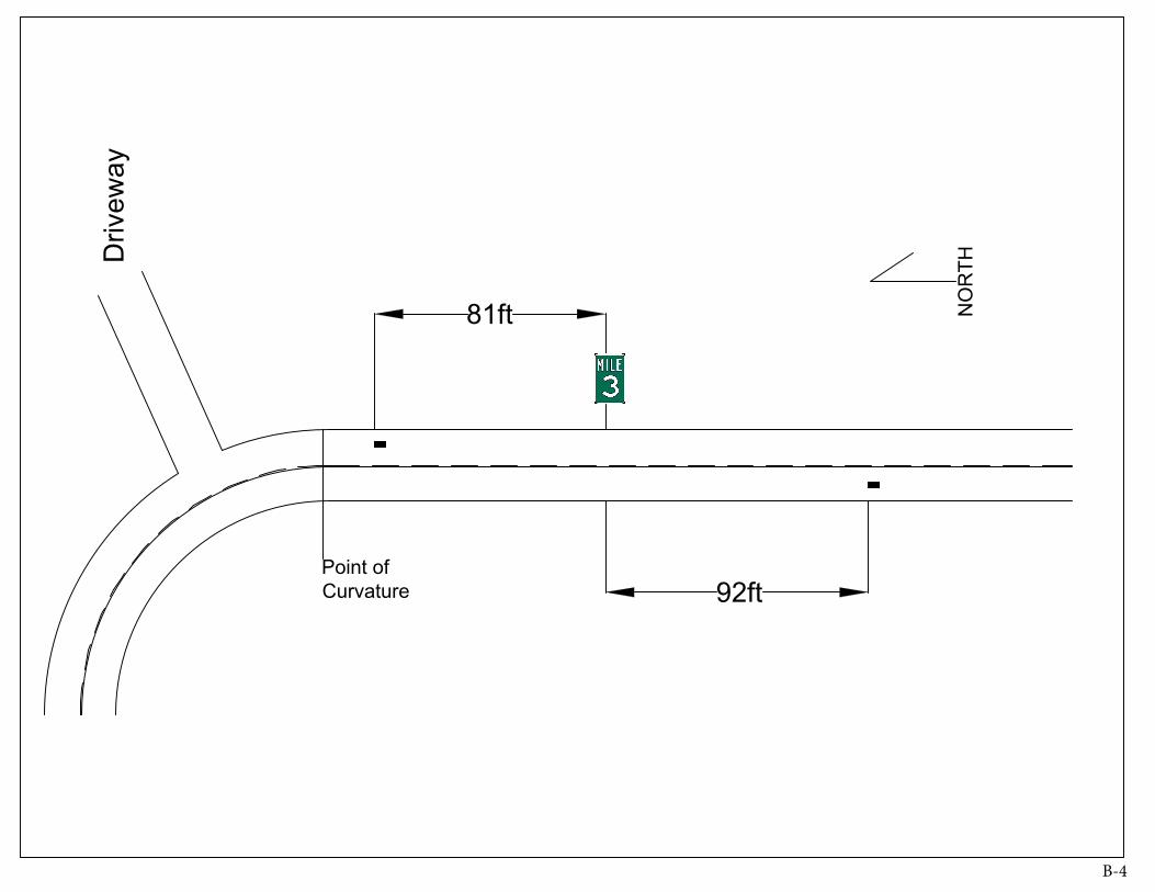
81ft

92ft

Driv

eway

Point ofCurvature

NO

RTH

B-4

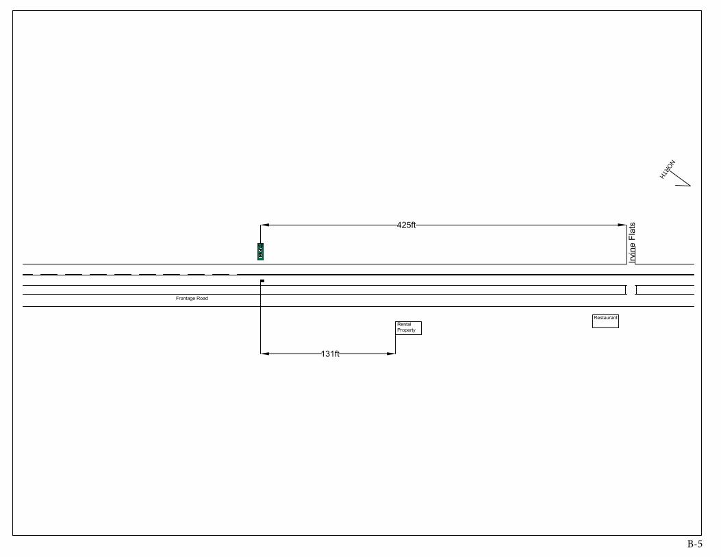
Irvin

e Fl

ats

Restaurant

Frontage Road

425ft

RentalProperty

131ft

NORTH

B-5

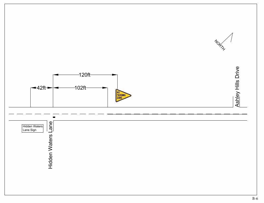
Hid

den

Wat

ers

Lane

Ash

ley

Hill

s D

rive

120ft

42ft 102ft

Hidden WatersLane Sign

NORTH

B-6

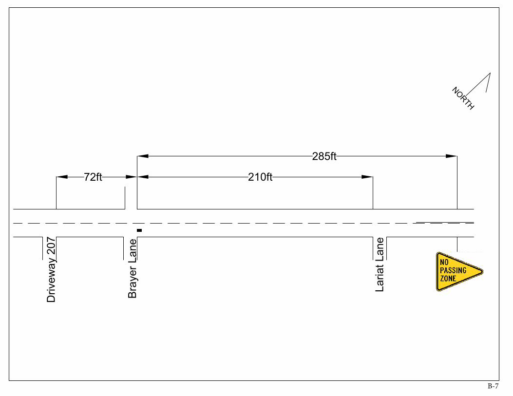
Laria

t Lan

e

Bra

yer L

ane

Driv

eway

207

72ft

285ft

210ft

NORTH

B-7

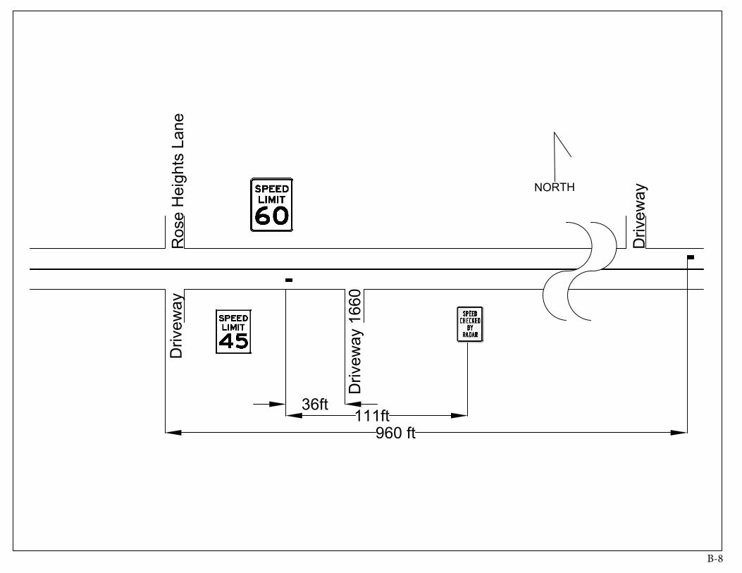
Driv

eway

Driv

eway

166

0

Ros

e H

eigh

ts L

ane

111ft36ft

NORTH

960 ft

Driv

eway

B-8

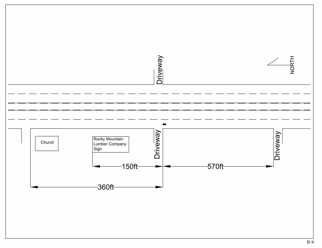
Driv

eway

Driv

eway

Driv

eway

ChurchRocky MountainLumber CompanySign

360ft

570ft150ft

NO

RTH

B-9

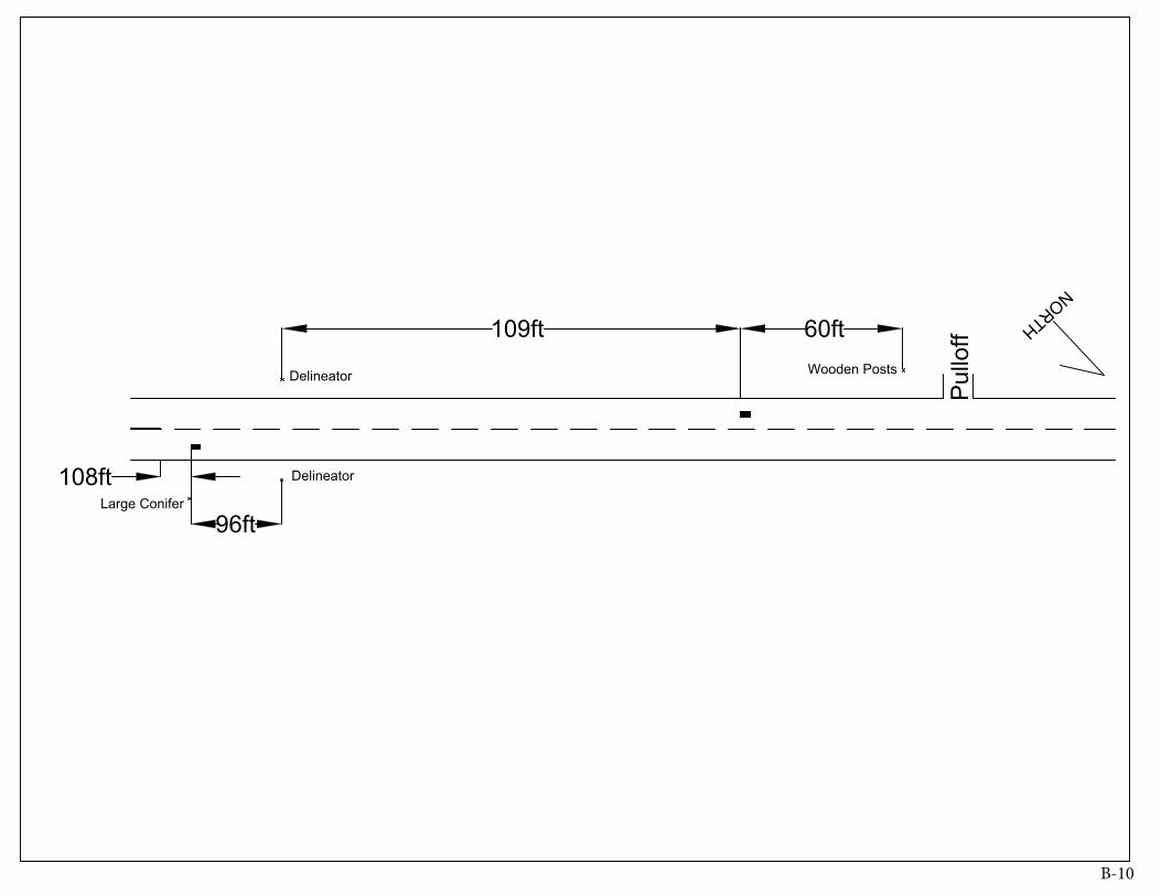
Pul

loff

Wooden Posts

Delineator

Delineator

Large Conifer

109ft 60ft

108ft

96ft

NORTH

B-10

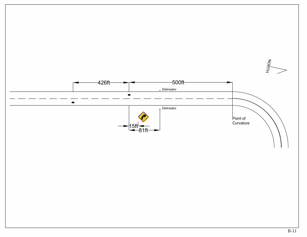
500ft

15ft81ft

Point ofCurvature

Delineator

Delineator

426ft

NO

RTH

B-11

Delineator

Pulloff

118ft

60ft

36ft

280ft153ft

66ft

NORTH

B-12

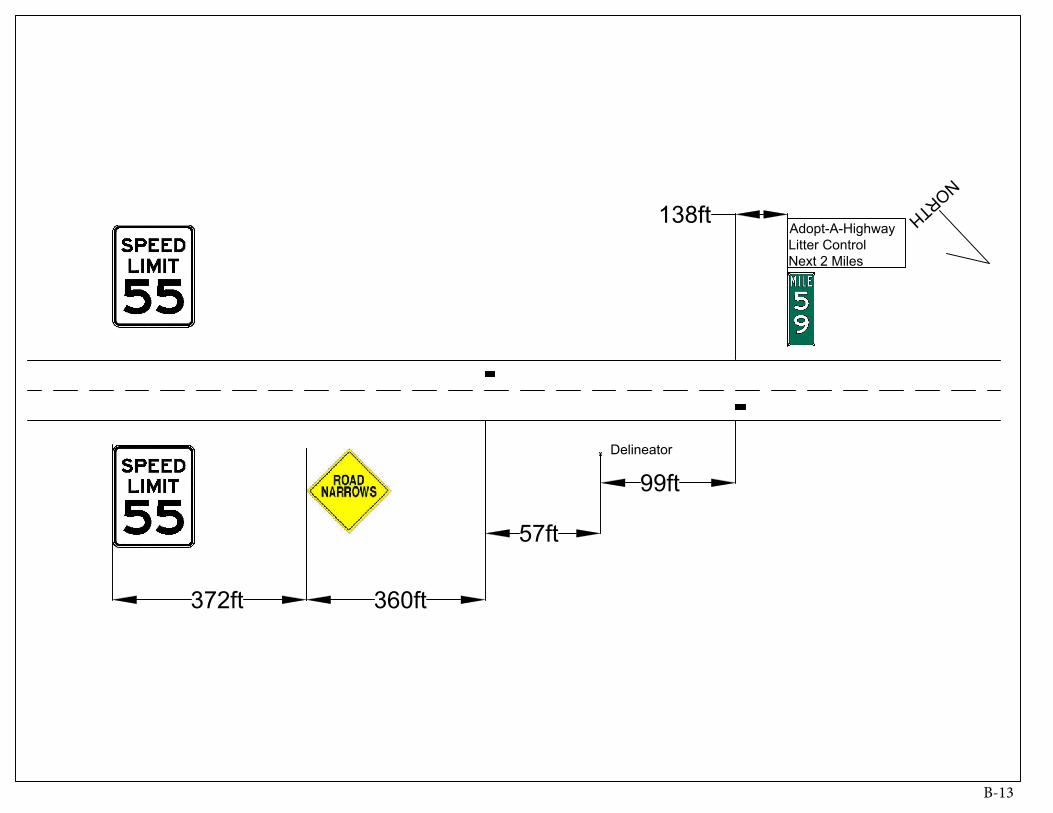
Adopt-A-HighwayLitter ControlNext 2 Miles

Delineator

138ft

99ft

57ft

360ft372ftNORTH

B-13

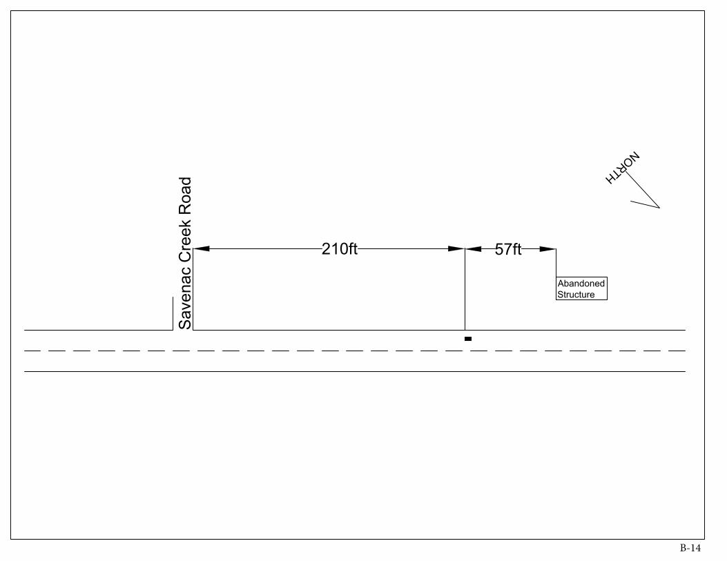
AbandonedStructure

Sav

enac

Cre

ek R

oad

57ft210ft

NORTH

B-14

Driv

eway

Driv

eway

Driv

eway

Driveway

36ft90ft

63ft

106ft

54ft21ft

Tree

NORTH

B-15

DrivewayDriveway

Old

Bro

adw

ater

Lane



57ft

195ft

78ft

Driveway

NORTH

B-16

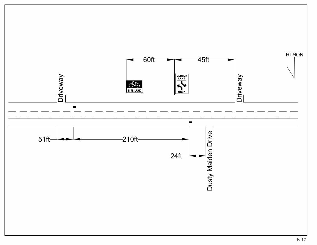
45ft

24ft

210ft

60ft

51ft

Dus

ty M

aide

n D

rive

Driv

eway

Driv

eway

NORTH

B-17

Bal

dy D

rive

Driv

eway

Driv

eway

126ft

24ft

93ft

42ft

120ft

60ft

NORTH

B-18

UtilityPole

Delineator

Delineator

111ft 159ft

120ft

33ft

30ft84ft

180ft100ft 30ft

Driv

eway

Driv

eway

Driv

eway

Driv

eway

NORTH

B-19

Delineator

Delineator

210ft75ft

120ft

123ft 231ft

63ft

Ste

lla B

lue

Driv

e

Ste

lla B

lue

Driv

e

Wes

t Acr

es L

oop

Driv

eway

NORTH

B-20

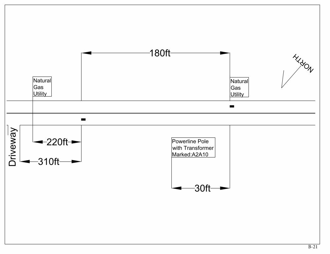
NaturalGasUtility

NaturalGasUtility

Powerline Polewith TransformerMarked:A2A10

180ft

220ft

310ft

30ft

Driv

eway

NORTH

B-21

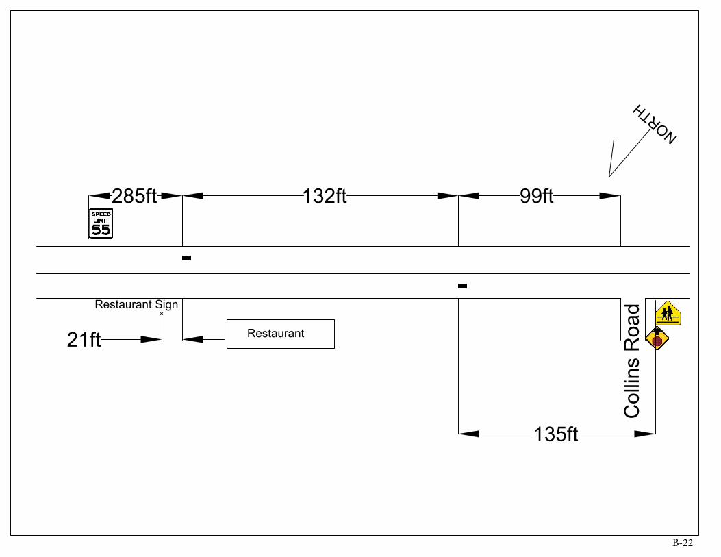
Col

lins

Roa

d

Restaurant

Restaurant Sign

21ft

135ft

285ft 132ft 99ft

NORTH

B-22

Driv

eway

#12

2

Driv

eway

#13

0

Delineator

165ft

334ft

30ft

NORT

H

B-23

This public document was published in electronic

format at no cost for printing and distribution.

Documents

Speed Limits Set Lower Than Engineering …...SPEED LIMITS SET LOWER THAN ENGINEERING RECOMMENDATIONS Final Report Prepared by: Eric T. Donnell Professor Vikash V. Gayah Assistant