Embed Size (px)
Citation preview

Speech Recognition Using
Features Extracted from Phase Space
Reconstructions
by
Andrew Carl Lindgren, B.S.
A THESIS
SUBMITTED TO THE FACULTY OF THE GRADUATE SCHOOL
IN PARTIAL FULFILLMENT OF THE REQUIREMENTS
for the degree of
MASTER OF SCIENCE
Field of Electrical and Computer Engineering
Marquette University
Milwaukee, Wisconsin
May 2003

iii
Preface
A novel method for speech recognition is presented, utilizing nonlinear/chaotic signal
processing techniques to extract time-domain based, reconstructed phase space derived
features. By exploiting the theoretical results derived in nonlinear dynamics, a distinct
signal processing space called a reconstructed phase space can be generated where sali-
ent features (the natural distribution and trajectory of the attractor) can be extracted for
speech recognition. These nonlinear methodologies differ strongly from the traditional
linear signal processing techniques typically employed for speech recognition. To dis-
cover the discriminatory strength of these reconstructed phase space derived features, iso-
lated phoneme classification experiments are executed using the TIMIT corpus and are
compared to a baseline classifier that uses Mel frequency cepstral coefficient features,
which are the typical benchmark. Statistical methods are implemented to model these fea-
tures, e.g. Gaussian Mixture Models and Hidden Markov Models. The results demon-
strate that reconstructed phase space derived features contain substantial discriminatory
power, even though the Mel frequency cepstral coefficient features outperformed them on
direct comparisons. When the two feature sets are combined, improvement is made over
the baseline, suggesting that the features extracted using the nonlinear techniques contain
different discriminatory information than the features extracted from linear approaches.
These nonlinear methods are particularly interesting, because they attack the speech rec-
ognition problem in a radically different manner and are an attractive research opportu-
nity for improved speech recognition accuracy.

iv
Acknowledgments
There have been several people who encouraged, supported, and gave invaluable advice
to me during my graduate work. First, I thank my wife, Amy, for her love and support the
last two years. I appreciate the encouragement that my parents, in-laws, and friends have
given me. I would like to acknowledge my thesis committee: Mike Johnson, Richard
Povinelli, and James Heinen. I especially want to thank my advisor, Mike Johnson, for
his guidance and solid mentoring. Also, Richard Povinelli, for our vast and tireless dis-
cussions on the topic of this research. Finally, I am grateful to the members of the ITR
group, the Speech and Signal Processing Laboratory, and the KID Laboratory at Mar-
quette for our awesome, thought provoking debates.

v
Table of Contents
LIST OF FIGURES .....................................................................................................VIII
LIST OF TABLES .......................................................................................................... IX
LIST OF ACRONYMS ................................................................................................... X
1. INTRODUCTION..................................................................................................... 1
1.1 OVERVIEW OF SPEECH RECOGNITION TECHNOLOGY AND RESEARCH.................. 1
1.1.1 Speech processing for recognition.................................................................. 1
1.1.2 Historical background of ASR ........................................................................ 5
1.1.3 Current research in ASR................................................................................. 6
1.2 DESCRIPTION OF RESEARCH................................................................................. 6
1.2.1 Problem statement .......................................................................................... 6
1.2.2 Speech and nonlinear dynamics...................................................................... 7
1.2.3 Previous work in speech and nonlinear dynamics.......................................... 9
1.2.4 Summary ....................................................................................................... 10
2. BACKGROUND ..................................................................................................... 13
2.1 CEPSTRAL ANALYSIS FOR FEATURE EXTRACTION............................................... 13
2.1.1 Introduction to cepstral analysis .................................................................. 14
2.1.2 Mel frequency Cepstral Coefficients (MFCCs) ............................................ 17
2.1.3 Energy, deltas, and, delta-deltas................................................................... 18
2.1.4 Assembling the feature vector....................................................................... 19
2.2 STATISTICAL MODELS FOR PATTERN RECOGNITION............................................ 20
2.2.1 Gaussian Mixture Models ............................................................................. 20

vi
2.2.2 Hidden Markov Models................................................................................. 25
2.2.3 Practical issues ............................................................................................. 26
2.3 SUMMARY.......................................................................................................... 28
3. NONLINEAR SIGNAL PROCESSING METHODS ......................................... 29
3.1 THEORETICAL BACKGROUND AND TAKENS’ THEOREM ..................................... 29
3.2 FEATURES DERIVED FROM THE RPS................................................................... 33
3.2.1 The natural distribution ................................................................................ 33
3.2.2 Trajectory information.................................................................................. 34
3.2.3 Joint feature vector ....................................................................................... 36
3.3 MODELING TECHNIQUE AND CLASSIFIER............................................................ 38
3.3.1 Modeling the RPS derived features............................................................... 38
3.3.2 Modeling of the joint feature vector.............................................................. 39
3.3.3 Classifier ....................................................................................................... 41
3.4 SUMMARY.......................................................................................................... 41
4. EXPERIMENTAL SETUP AND RESULTS ....................................................... 42
4.1 SOFTWARE ......................................................................................................... 42
4.2 DATA ................................................................................................................. 43
4.3 TIME LAGS AND EMBEDDING DIMENSION ........................................................... 46
4.4 NUMBER OF MIXTURES....................................................................................... 48
4.5 BASELINE SYSTEMS............................................................................................ 49
4.6 DIRECT COMPARISONS ....................................................................................... 50
4.7 STREAM WEIGHTS .............................................................................................. 51
4.8 JOINT FEATURE VECTOR COMPARISON ............................................................... 53

vii
4.8.1 Accuracy results............................................................................................ 53
4.8.2 Statistical tests .............................................................................................. 53
4.9 SUMMARY.......................................................................................................... 54
5. DISCUSSION, FUTURE WORK, AND CONCLUSIONS................................. 55
5.1 DISCUSSION ....................................................................................................... 55
5.2 KNOWN ISSUES AND FUTURE WORK ................................................................... 56
5.2.1 Feature extraction......................................................................................... 56
5.2.2 Pattern recognition ....................................................................................... 58
5.2.3 Continuous speech recognition..................................................................... 59
5.3 CONCLUSIONS.................................................................................................... 59
6. BIBLIOGRAPHY AND REFERENCES ............................................................. 61
APPENDIX A – CONFUSION MATRICES ............................................................... 66
APPENDIX B – CODE EXAMPLES ........................................................................... 71

viii
List of Figures
Figure 1: Block diagram of speech production mechanism................................................ 2
Figure 2: Block diagram of ASR system ............................................................................ 4
Figure 3: Example of reconstructed phase space for a speech phoneme............................ 8
Figure 4: Block diagram of speech production model...................................................... 14
Figure 5: Block diagram of the source-filter model.......................................................... 15
Figure 6: Cepstral analysis for a speech phoneme............................................................ 16
Figure 7: Hamming window ............................................................................................. 17
Figure 8: Block diagram of feature vector computation................................................... 20
Figure 9: Visualization of a GMM for randomly generated data ..................................... 23
Figure 10: Diagram of HMM with GMM state distributions ........................................... 26
Figure 11: Two dimensional reconstructed phase spaces of speech phonemes................ 31
Figure 12: RPS of a typical speech phoneme demonstrating the natural distribution and
the trajectory information ......................................................................................... 35
Figure 13: Relationship between indices for the joint feature vector ............................... 37
Figure 14: GMM modeling of the RPS derived features for the phoneme '/aa/' .............. 38
Figure 15: Time lag comparison in RPS........................................................................... 46
Figure 16: False nearest neighbors for 500 random speech phonemes ............................ 47
Figure 17: Classification accuracy vs. number of mixtures for RPS derived features ..... 49
Figure 18: Accuracy vs. stream weight............................................................................. 52

ix
List of Tables
Table 1: List of notation used in section 2.1..................................................................... 13
Table 2: Notation used for section 2.2 .............................................................................. 20
Table 3: Notation for Chapter 3 ........................................................................................ 29
Table 4: Notation used in Chapter 4 ................................................................................. 42
Table 5: List of phonemes, folding and statistics ............................................................. 45
Table 6: Direct performance comparison of the feature sets ............................................ 51
Table 7: Comparisons for different stream weights.......................................................... 53
Table 9: Example of a confusion matrix........................................................................... 66
Table 10: Confusion matrix for ( )5,6nx ................................................................................ 67
Table 11: Confusion matrix for ( )10,6nx ............................................................................... 67
Table 12: Confusion matrix for ( )5,6,& fdnx ........................................................................... 68
Table 13: Confusion matrix for ( )5,6,&n
∆x ............................................................................ 68
Table 14: Confusion matrix for ct .................................................................................... 69
Table 15: Confusion matrix for Ot ................................................................................... 69
Table 16: Confusion matrix for , 0n ρ =y ........................................................................ 70
Table 17: Confusion matrix for , 0 .25n ρ =y .................................................................. 70

x
List of Acronyms
ANN Artificial Neural Networks
ASR Automatic Speech Recognition
DCT Discrete Cosine Transform
DFT Discrete Fourier Transform
DTW Dynamic Time Warping
EM Expectation Maximization
FFT Fast Fourier Transform
GMM Gaussian Mixture Model
HMM Hidden Markov Model
HTK Hidden Markov Modeling Toolkit
IDFT Inverse Discrete Fourier Transform
LPC Linear Predicative Coding
MFCC Mel Frequency Cepstral Coefficients
PDF Probability Density Function
RPS Reconstructed Phase Space
TIMIT Texas Instruments & Massachusetts Institute of Technology speech corpus
Z Z Transform

1
1. Introduction
1.1 Overview of Speech Recognition Technology and Research
1.1.1 Speech processing for recognition
Speech processing is the mathematical analysis and application of electrical signals
for information storage and/or retrieval that results from the transduction of acoustic
pressure waves gathered from human vocalizations. The teleology of speech processing
generally can be subdivided into the broad overlapping categories of speech analysis,
coding, enhancement, synthesis and recognition. Speech analysis is the study of the
speech production mechanism in order to generate a mathematical model of the physical
phenomena. The study of coding endeavors to store speech information for subsequent
recovery. Enhancement, in contrast, is the process of improving the intelligibility and
quality of noise-corrupted speech signals. The generation of speech from coded instruc-
tions is known as speech synthesis. Speech recognition, though, is the process of synthe-
sis in reverse; namely, given a speech signal, produce the code that generated it. Speech
recognition is the task that will be addressed in this work.
For the vast majority of applications, the code that speech recognition systems strive
to identify is the units of language, usually phonemes (set of unique sound categories for
a language) or words, which can be compiled into text [1]. Speech recognition can then
be formulated as a decoding problem, where the goal is to map speech signals to their
underlying textual representations. The potential applications of automatic speech recog-
nition (ASR) systems include computer speech-to-text dictation, automatic call routing,
and machine language translation. ASR is a multi-disciplinary area that draws theoretical
knowledge from mathematics, physics, engineering, and social science. Specific topics

2
include signal processing, information theory, random processes, machine learning / pat-
tern recognition, psychoacoustics, and linguistics.
The development of speech recognition systems begins with the processing of a
given speech signal for the purposes of obtaining the discriminatory acoustic information
about that utterance. The discriminatory information is represented by computed numeri-
cal quantities called features. Current speech processing techniques are based on model-
ing speech as a linear stochastic process [2].The underlying speech production model is
what is known as a source-filter model, where the vocal tract is excited by a series of
pitch pulses (e.g. vowels) or Gaussian white noise (e.g. fricatives), which ultimately re-
sults in certain frequency spectra that humans recognize as sounds [2].
EXCITATION FROM VOCAL FOLDS
MOUTH
VOCALCORDS
TRACHEA
LUNGS
LARYNX
PHARYNX
NOSE
SPEECH
VOCAL TRACTFILTER SPEECHEXCITATION FROM
VOCAL FOLDS
MOUTH
VOCALCORDS
TRACHEA
LUNGS
LARYNX
PHARYNX
NOSE
SPEECH
MOUTH
VOCALCORDS
TRACHEA
LUNGS
LARYNX
PHARYNX
NOSE
SPEECH
VOCAL TRACTFILTER SPEECH
Figure 1: Block diagram of speech production mechanism

3
Features are extracted with the goal of capturing the characteristic frequency spectrum of
a particular phoneme. One feature set typically used in ASR are cepstral coefficients
(usually Mel frequency cepstral coefficients) [2]. Using the acoustic features, speech
recognition algorithms are employed to accomplish the undertaking. The process starts at
the phoneme or acoustic level where consecutive, overlapping, short portions (called
frames) of speech (~10-30 ms) are assumed to be approximately stationary, and fre-
quency domain-based features are extracted such as Mel frequency cepstral coefficients
(MFCCs) [2].
Following feature extraction, machine learning techniques are employed to use the
features for recognition. There are many machine learning algorithms that can be utilized
for the speech recognition task. A common approach is to use statistical pattern recogni-
tion methodologies.
In this paradigm, a probability density function (PDF) of these features is generated
from the training examples [2-5]. The PDF is usually a continuous, parametric function
that is a sum of weighted Gaussian functions, which is called a Gaussian Mixture Model
(GMM). In order to track the rapid changes of the vocal tract as a human utters several
sounds (phonemes) consecutively, another model must be employed called a Hidden
Markov Model (HMM). A HMM is finite state machine where each state has an associ-
ated GMM which represents one possible configuration of the vocal tract. HMMs also
have parameters called transition probabilities that represent the likelihood of transition-
ing from one vocal tract configuration to another. The parameters of these statistical
models are learned or optimized using training data.

4
After model training is complete, previously unseen test data is presented to the rec-
ognizer. The recognizer outputs the most likely language units associated with that test
data given the trained models. A more detailed and mathematically rigorous explanation
of ASR systems will be given in subsequent chapters.
The pattern recognition algorithms utilized must be robust to the inherent variabili-
ties of speech such as changing speech rates, coarticulation effects, different speakers,
and large vocabulary sizes[1, 2]. Other knowledge sources that have discriminatory
power, in addition to the acoustic data, can also be incorporated into the recognizer such
as language models. The final output of the system can be the single phoneme, a se-
quence of phonemes, an isolated word, an entire sentence, etc. depending on the specific
application and problem domain.
Accuracy Evaluation
(5)
Parameter Learning
(2)
Databases
Feature Extraction
(1)
Recognition
(4)
Parameters
(3)
Figure 2: Block diagram of ASR system

5
1.1.2 Historical background of ASR
The first speech recognition system was built at Bell Labs in the early 1950’s [1]. The
task of the system was to recognize digits separated by pauses spoken from a single
speaker. The system was built using analog electronics and it performed recognition by
detecting the resonant frequency peaks (called formants) of the uttered digit. Despite its
crudeness, the system was able to achieve 98% accuracy, and it proved the concept that a
machine could recognize human speech [1].
Research continued into the 1960’s and 1970’s fueled by the advent of digital com-
puting technology with focus both on the signal processing and the pattern recognition
aspects of developing a speech recognizer. The most significant contributions to speech
analysis included to the development of the Fast Fourier Transform (FFT), cepstral
analysis, and linear predictive coding (LPC), which replaced the antiquated method of
filter banks used in the past. Pattern recognition algorithms such as artificial neural net-
works (ANN), dynamic time warping (DTW), and Hidden Markov Models (HMM) were
successfully applied to speech. These methodologies resulted in several functional and
useful systems for a variety of applications [1].
In the 1980’s and early 1990’s, research focused on expanding the capabilities of
ASR systems to more complex tasks including speaker independent data sets, larger vo-
cabularies, and noise robust recognition. Progress was made by incorporating speech-
tailored signal processing methods for feature extraction such as Mel frequency cepstral
coefficients (MFCC). HMM methods were further refined and became the prevailing
ASR technology. Also, the research community became more organized for facilitation
of data and software sharing so that comparisons among researchers could be made.

6
Standard speech data was compiled and distributed such as the TIMIT corpus and the Re-
source Management corpus. Also, speech software toolkits with open source code were
made available; the Hidden Markov Modeling Toolkit (HTK) being one example [5]. The
period was punctuated by the release of several commercial products; the most famous
being personal computer dictation systems including IBM ViaVoice and Dragon Sys-
tems Naturally Speaking [1].
1.1.3 Current research in ASR
Current research efforts are focused on several different task dependent categories as
well as on the different aspects of ASR systems. The task complexities include speaker
independent data sets, large vocabulary recognition, spontaneous speech recognition,
noise robust recognition, and speaker verification / identification. Additionally, new
methodologies have been under investigation, such as rapid speaker adaptation, discrimi-
native training techniques, vocal tract normalization, multi-modal ASR, and improved
language modeling. Despite the increased popularity of ASR as a research area, progress
over the last 10-15 years has been largely incremental. Most of the ASR literature that
describes and implements new methods report small improvements (< 3% increased ac-
curacy) over baseline recognizers on standard corpora.
1.2 Description of Research
1.2.1 Problem statement
The problem addressed in this thesis concerns the investigation of novel acoustic
modeling techniques that exploit the theoretical results of nonlinear dynamics, and ap-
plies them to the problem of speech recognition. The assessment of ASR systems is
driven by results and this concept reduces the problem to the following question: “Does

7
the use of nonlinear signal processing techniques improve the accuracy of current state-
of-the-art (baseline) computer speech-to-text systems?” Although this is the central ques-
tion addressed in this work, this research also seeks to further the understanding of the
nonlinear methods employed, as well as to ascertain the limitations of the current tech-
niques conventionally used in ASR. In summary, therefore, this research will endeavor to
boost the results of current methodologies, while concurrently extending the knowledge
of these new nonlinear techniques.
1.2.2 Speech and nonlinear dynamics
There are two distinct but related research fields that are addressed in this work:
nonlinear dynamics and speech recognition. In the nonlinear dynamics community, a
budding interest has emerged in the application of theoretical results to experimental time
series data; the most significant being Takens’ Theorem and Sauer and Yorke’s extension
of this theorem [6, 7]. Takens’ theorem states that under certain assumptions, the state
space (also called phase space or lag space) of a dynamical system can be reconstructed
through the use of time-delayed versions of the original signal. This new state space is
commonly referred to in the literature as a reconstructed phase space (RPS), and has been
proven to be topologically equivalent to the original phase space of the dynamical sys-
tem, as if all the state variables of that system would have been measured simultaneously
[6, 7]. A RPS can be exploited as a powerful signal processing domain, especially when
the dynamical system of interest is nonlinear or even chaotic [8, 9]. Conventional linear
digital signal processing techniques often utilize the frequency domain as the primary
processing space, which is obtained through the Discrete Fourier Transform (DFT) of a
time series [10]. For a linear dynamical system, structure appears in the frequency do-
8
main that takes the form of sharp resonant peaks in the spectrum. However for a nonlin-
ear or chaotic system, structure does not appear in the frequency domain, because the
spectrum is usually broadband and resembles noise [8]. In the RPS, though, structure
does emerge in the form of complex, dense orbits that form patterns known as attractors.
These attractors contain the information about the time evolution of the system, which
means that features derived from a RPS can potentially contain more and/or different in-
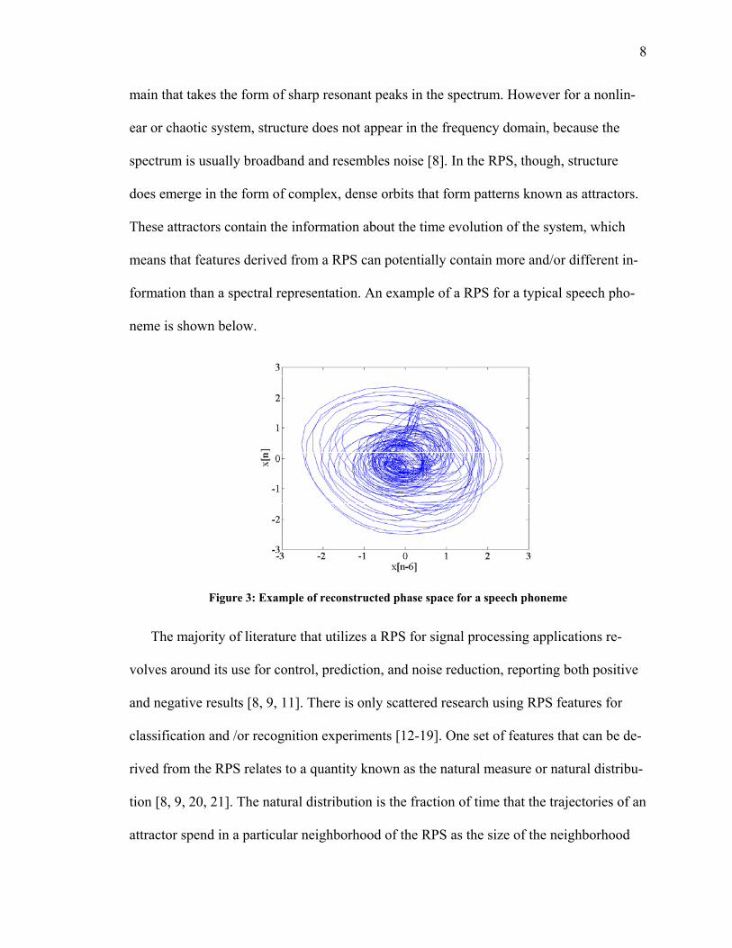
formation than a spectral representation. An example of a RPS for a typical speech pho-
neme is shown below.
Figure 3: Example of reconstructed phase space for a speech phoneme
The majority of literature that utilizes a RPS for signal processing applications re-
volves around its use for control, prediction, and noise reduction, reporting both positive
and negative results [8, 9, 11]. There is only scattered research using RPS features for
classification and /or recognition experiments [12-19]. One set of features that can be de-
rived from the RPS relates to a quantity known as the natural measure or natural distribu-
tion [8, 9, 20, 21]. The natural distribution is the fraction of time that the trajectories of an
attractor spend in a particular neighborhood of the RPS as the size of the neighborhood

9
goes to zero and time goes to infinity, or simply the distribution of points in the RPS [22].
For an experimental time series such as speech, the signal is of finite length so the natural
distribution can only be estimated via a numerical algorithm or model. Previous work has
shown that accurate estimates of the natural distribution can be obtained through both
histogram methods and Gaussian Mixture Models [12, 17]. This work has demonstrated
that estimations of the natural distribution can be robust, accurate, and useful for recogni-
tion/classification, which is the central focus of this thesis.
1.2.3 Previous work in speech and nonlinear dynamics
There have been only a few publications that have examined the possibilities of ap-
plying nonlinear signal processing techniques to speech, all of which have been published
within the last ten years [12-15, 18, 23-34]. Work by Banbrook et al. [23], Kumar et al.
[27], and Narayanan et al. [31] has attempted to use nonlinear dynamical methods to an-
swer the question: “Is speech chaotic?” These papers focused on calculating theoretical
quantities such as Lyapunov exponents and Correlation dimension. Their results are
largely inconclusive and even contradictory. Other papers by Petry et al. and Pitsikalis et
al. have used Lyapunov exponents and Correlation dimension in unison with traditional
features (cepstral coefficients) and have shown minor improvements over baseline speech
recognition systems. Central to both sets of these papers is the importance of Lyapunov
exponents and Correlation dimension, because they are invariant metrics that are the
same regardless of initial conditions in both the original and reconstructed phase space
[8]. Despite their significance, there are several issues that exist in the measuring of these
quantities on real experimental data. The most important issue is that these measurements
are very sensitive to noise [35]. Secondarily, the automatic computation of these quanti-

10
ties through a numerical algorithm is not well established and this can lead to drastically
differing results. The overall performance of these quantities as salient features remains
an open research question.
In addition to these speech analysis and recognition applications, nonlinear methods
have also been applied to speech enhancement. Papers by Hegger et al. [24, 25] demon-
strated the successful application of what is known as local nonlinear noise reduction to
sustained vowel utterances. In our previous work [13], we extended this algorithm into a
complete speech enhancement algorithm. The results showed mild success and demon-
strated some of the potential limitations of the algorithm despite the optimistic claims
made in the papers by Hegger et al.
With the exception of our work [12], the use of the natural distribution as a feature set
derived from the RPS is yet to be exploited for speech recognition, which is the primary
focus of this thesis.
1.2.4 Summary
As described, nonlinear signal processing techniques have several potential advan-
tages over traditional linear signal processing methodologies. They are capable of recov-
ering the nonlinear dynamics of the signal of interest possibly preserving more and /or
different information. Furthermore, they are not constrained by strong linearity assump-
tions. Despite these facts, the use of nonlinear signal processing techniques also have dis-
advantages as well, which is why they have not been widely used in the past. Primarily,
they are not as well understood as conventional linear methods. Additionally, the RPS
can be difficult to interpret, because little is understood in the way of attaching physical
meaning to particular attractor characteristics that appear in the RPS. Salient features for
11
classification/recognition have yet to be firmly established, and this work is clearly in the
early stages, which is what motivates this research pursuit. Moreover, researchers have
just begun to study nonlinear signal processing techniques for a variety of engineering
tasks with mixed success. The use of nonlinear methodologies especially as it applies to
speech recognition is truly in its infancy with very little work published, most of which
has been in the last three years. Therefore, this thesis constitutes some of the very first
work performed on the subject.
In order to ascertain the feasibility of the nonlinear techniques, discover the discrimi-
natory power of the RPS derived features, and expand the knowledge of these nonlinear
signal processing methods, work was conducted on the task of isolated phoneme classifi-
cation. The motivation for restricting the scope of the research to isolated phoneme clas-
sification was two-fold. The first reason is that isolated phoneme classification allows
one to focus in on the performance of the features, because the classification is performed
using the acoustic data alone, and in turn, makes comparisons among different feature
sets as “fair” as possible. Secondly, the task is less complex than continuous speech rec-
ognition, where issues of phoneme duration modeling create additional difficulties. The
topic of phoneme duration will be discussed in full detail later.
The statistical model employed in this work was a one state Hidden Markov Model
with a Gaussian Mixture Model state distribution. Again, this model was chosen to make
comparisons “reasonable” and to keep the focus on the acoustic data.
Experiments were performed on both baseline MFCC feature sets, RPS derived fea-
ture sets, and joint MFCC and RPS feature sets. The choice of these feature sets allows

12
investigation into the discriminatory and representational power of each set as well as the
sets used in unison.
The remainder of the thesis is outlined as follows. Chapter 2 summarizes conven-
tional methods used in speech recognition, namely cepstral analysis and the statistical
models typically used in speech: Hidden Markov Models and Gaussian Mixture Models.
Chapter 3 develops the nonlinear methods employed in this research along with the fea-
ture extraction schemes utilized. Chapter 4 describes the experimental setup and the re-
sults of this work. Finally, Chapter 5 details the discussion of the results, draws conclu-
sions, and proposes several different possible future research avenues in this area.

13
2. Background 2.1 Cepstral analysis for feature extraction
n time index
[ ]s n signal in the time domain
[ ]e n excitation signal in the time domain
[ ]h n linear time invariant filter in time domain
[ ]fs n frame of a signal in time do-main
ω frequency index
( )S ω signal in the frequency domain
( )E ω excitation signal in the fre-quency domain
( )H ω linear time invariant filter in frequency domain
( )fS ω frame of a signal in the fre-quency domain
q quefrency index
( )C q cepstral coefficients in the que-frency domain
melF Mel frequency scale
HzF linear frequency scale
t index of frames
c MFCC of a frame
E energy measure
∆ delta vector
∆∆ delta-delta vector
O composite feature vector
Table 1: List of notation used in section 2.1

14
2.1.1 Introduction to cepstral analysis
The aim of cepstral analysis methods is to extract the vocal tract characteristics from
the excitation source, because the vocal tract characteristics are what contain the informa-
tion about the phoneme utterance [2]. Cepstral analysis is a form of homomorphic signal
processing, where nonlinear operations are used to give the equations the properties of
linearity [2].
One typical model used to represent the entire speech production mechanism is given
in figure below.
Impulse Generator
GlottalFilter
Noise Generator
Gain
Gain
Vocal Tract Filter
Lip Radiation
FilterUnvoiced
Voiced
Switch
Speech Signal
Impulse Generator
GlottalFilter
Noise Generator
Gain
Gain
Vocal Tract Filter
Lip Radiation
FilterUnvoiced
Voiced
Switch
Speech Signal
Figure 4: Block diagram of speech production model
Although this model is accurate, the analysis can be made simpler by replacing the glot-
tal, vocal tract, and lip radiation filters, by a single vocal tract filter given in the next fig-
ure. This model is obtained by collapsing all these separate filters into a vocal tract filter
by the convolution operation.

15
EXCITATION FROM VOCAL FOLDS
VOCAL TRACTFILTER
SPEECHEXCITATION FROM VOCAL FOLDS
VOCAL TRACTFILTER
SPEECH
Figure 5: Block diagram of the source-filter model
An analytical model of this block diagram can be formulated in the following way.
According to the conventional source-filter model representation, a speech signal is com-
posed of an excitation source convolved with the vocal tract filter.
[ ] [ ] [ ]{ }
( ) ( ) ( )DFT
s n h n e n S H Eω ω ω= ∗ =⇒i
(2.1.1)
By taking the logarithm of the magnitude of both sides, the equation is converted from a
multiplication to an addition.
( ) ( ) ( ) ( ) ( )log log log logS H E H Eω ω ω ω ω= = + (2.1.2)
Then, by taking the inverse discrete Fourier Transform (IDFT) of ( )log S ω , the cep-
strum is obtained in what is known as the quefrency domain [2].
( ) { } ( ){ } ( ){ }log ( ) log logC q IDFT S IDFT H IDFT Eω ω= = + ω (2.1.3)
The cepstrum then allows the excitation signal to be completely isolated from the vo-
cal tract characteristics, because the multiplication in the frequency domain has been
converted to an addition in the quefrency domain.
A visual demonstration of the computation of the cepstrum for a frame of speech data
is shown in the following figure. Notice that the ripple in log spectral magnitude, which
is due to the excitation source, is isolated from the spectral envelope of the vocal tract.

16
Figure 6: Cepstral analysis for a speech phoneme
Cepstral coefficients, C q , can be used as features for speech recognition for sev-
eral reasons. First, they represent the spectral envelope, which is the vocal tract. The vo-
cal tract characteristics are understood to contain information about the phoneme that is
produced. Second, cepstral coefficients have the property that they are uncorrelated with
one another, which simplifies subsequent analysis [1, 2]. Third, their computation can be
done in a reasonable amount of time. The last and most important reason is that cepstral
coefficients have empirically demonstrated excellent performance as features for speech
recognition for many years [2].
( )

17
2.1.2 Mel frequency Cepstral Coefficients (MFCCs)
The most popular form of cepstral coefficients are known as Mel frequency cepstral
coefficients (MFCCs). MFCCs are computed in a similar way as the methods described
in section 2.1.1, but have been slightly modified. The procedure is as follows:
a) The signal is filtered using a pre-emphasis filter to accentuate the high-
frequency content. This is also performed to compensate for the spectral tilt
that is present in most speech phoneme spectra.
(2.1.4) [ ] [ ] [ ]{ }
( ) ( ) ( )Z
f f fs n h n s n S z H z S z′ ′= ∗ ⇒ =i
f
( ) 11 0.97H z z−= − (2.1.5)
b) The signal is multiplied by overlapping windows and divided into frames
usually using ~20-30 ms windows with ~10-15ms of overlap between win-
dows.
[ ] [ ] [ ]f fs n s n w n′′ ′= ⋅ (2.1.6)
A hamming window is typically used for [ ]w n .
[ ] ( )0.54 0.46cos 2 / , 00, otherwise
n N n Nw n
π − ≤=
≤ (2.1.7)
0 100 200 300 400 5000
0.1
0.2
0.3
0.4
0.5
0.6
0.7
0.8
0.9
1
time index Figure 7: Hamming window

18
c) The discrete Fourier Transform (DFT) is taken of every frame ( )fs′′ followed
by the logarithm.
( ) [ ]{ }logfS DFT sω′′′ ′′= f n (2.1.8)
d) Twenty-four triangular-shaped filter banks with approximately logarithmic
spacing (called Mel banks) are applied to ( )fS ω′′′ . The energy in each of these
bands is integrated to give 24 coefficients in the spectrum. The Mel scale is a
warping of the frequency axis that models the human auditory system and
has been shown to empirically improve recognition accuracy. A curve fit is
usually used to approximate the empirically derived scale given below.
102595log 1700
Hzmel
FF = +
(2.1.9)
e) The Discrete Cosine Transform (DCT) is taken to give the cepstral coeffi-
cients.
( ){ }c DCT S ω′′′= (2.1.10)
f) The first 12 coefficients (excluding the 0th coefficient) are the features that
are known as MFCCs ( )tc .
2.1.3 Energy, deltas, and, delta-deltas
In addition to MFCC’s, typically other elements are appended to the feature vector.
One prominent measure is the energy. The energy can be an important metric for distin-
guishing among different phonemes [5]. Although the 0th cepstral coefficient can be used

19
as an energy measure, it is usually preferred to use the energy in the framed time series as
given below.
(2.1.11) [ ]2
1log
N
fn
E s=
′= ∑ n
The temporal change of cepstral coefficients over a sequence a frames is also a valu-
able feature. This temporal change or derivative has boosted the accuracy of ASR sys-
tems for many applications [3, 12]. One way to estimate the derivative of the MFCCs is
to use a simple linear regression formula [5].
( )
1
2
12
t t
t
θ θθ
θ
θ
θ
Θ
+ −=
Θ
=
−∑=
∑∆
c c (2.1.12)
The second derivatives are estimated simply by taking the linear regression formula given
in equation (2.1.12) and applying to t∆ [5].
( )
1
2
12
t t
t
θθ
θ
θ
θ
Θ
+ −=
Θ
=
−∑=
∑
∆ ∆∆∆
θ
tE
(2.1.13)
These derivative estimates are refered to as deltas and delta-deltas respectively. The de-
rivative estimates of the energy are computed using the same formulas as for the MFCCs.
2.1.4 Assembling the feature vector
After all the analysis is performed on every frame, the computed elements can be
compiled into a feature vector (given below) and then as input to an ASR system.
| | | | |t t tEt t t t t t tE=
c cO c ∆ ∆ ∆∆ ∆∆ (2.1.14)
The feature vector is composed as follows: i.) 12 MFCCs ii.) energy iii.) deltas of the 12
MFCCs iv.) delta of the energy v.) delta-deltas of the 12 MFCCs vi.) delta-delta of the

20
energy. The total number of elements in the feature vector is then 39. A illustration of the
the computation of the feature in block diagram form is displayed next.
Speech Signal
Energy Measure
Windowed FFT
DCT 12 CepstralCoefficients
. . .
Mel-spaced Filterbanks
Deltas and delta-deltas
39 Element Feature Vector
Figure 8: Block diagram of feature vector computation
2.2 Statistical models for pattern recognition 2.2.1 Gaussian Mixture Models
( )p i probability density function
x an arbitrary feature vector
m mixture index
w mixture weight
µ mean vector
∑ covariance matrix
k index of training vectors
λ set of parameters of a statistical model
i iterative index
ω class
c class index
q index of testing vectors
Table 2: Notation used for section 2.2

21
The first step in building a statistical pattern recognition system is choosing an appro-
priate model to capture the distribution of the underlying features. Gaussian Mixture
Models (GMM) are an excellent choice, because they have several desirable properties.
Their primary advantage is that they are flexible and robust, because they can accurately
model a multitude of different distributions including multi-modal data. In fact, they can
represent any arbitrary probability density function (PDF) in the limit as the number of
mixtures go to infinity [36]. The equations for a GMM are given below. (M → ∞)
( ) (1
M
mm
)p w p m=
= ∑x x (2.2.1)
( ) ( ) ( ) ( ) (1 † 122
12 exp ; ,2
d
m m m mp m Nπ −− − = − − − =
x Σ x )m mµ Σ x µ x µ Σ (2.2.2)
Frequently, there is no prior knowledge of the distribution of the data and consequently, a
GMM will be a suitable model for the task.
After the model has been chosen, the parameters of that PDF have to be learned from
training data. The typical data-driven method used to estimate these model parameters is
to discover the parameters that maximize the data likelihood, known as the Maximum
Likelihood method. Assuming that the data points (feature vectors) are statistically inde-
pendent from one another, the objective or criterion function can be formulated known as
the likelihood function ( or the log likelihood function ) ( )L .
( ) ( )11log
K K
kkk
p L p==
= ⇒ = ∑∏ x kx (2.2.3)
This objective function is optimized through the well-known Expectation Maximization
(EM) algorithm [36-38]. EM Maximization is usually formulated as a “missing data”
problem. The missing information in the case of a GMM is what mixture component a
22
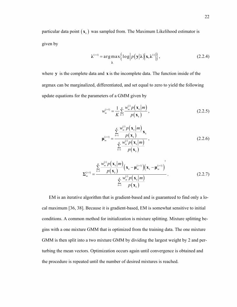
particular data point was sampled from. The Maximum Likelihood estimator is
given by
( kx )
( ) ( ) ( ){ }1 arg max log , ,i p+ =λ
λ y λ x λ i (2.2.4)
where y is the complete data and is the incomplete data. The function inside of the
argmax can be marginalized, differentiated, and set equal to zero to yield the following
update equations for the parameters of a GMM given by
x
( )( ) ( )
( )1
1
1 ,i
K m kim
kk
w p mw
K p+
== ∑
xx
(2.2.5)
( )
( ) ( )( )
( ) ( )( )
11
1
,
iK m k
kki k
m iK m k
kk
w p mp
w p mp
=+
=
∑=
∑
xx
xµ
xx
(2.2.6)
( )
( ) ( )( )
( )( ) ( )( )( ) ( )
( )
†
1 1
11
1
.
iK m k i i
k m k mki k
m iK m k
kk
w p mp
w p mp
+ +
=+
=
− −∑=
∑
xx µ x µ
xΣ
xx
(2.2.7)
EM is an iterative algorithm that is gradient-based and is guaranteed to find only a lo-
cal maximum [36, 38]. Because it is gradient-based, EM is somewhat sensitive to initial
conditions. A common method for initialization is mixture splitting. Mixture splitting be-
gins with a one mixture GMM that is optimized from the training data. The one mixture
GMM is then split into a two mixture GMM by dividing the largest weight by 2 and per-
turbing the mean vectors. Optimization occurs again until convergence is obtained and
the procedure is repeated until the number of desired mixtures is reached.

23
In addition to EM’s sensitivity to initial conditions, there is no well-established
method for setting the number of mixtures in a GMM. The number of mixtures in the
GMM is related to the complexity of the model and data; the more mixtures in the GMM
the more complex the model, and consequently, the more complex the data distribution.
Care must be taken in setting the number of mixtures; too few mixtures can lead to in-
adequate representations of the data, ultimately resulting in poor classification accuracy.
Too many mixtures leads to over-fitting and data memorization, which results in high
training accuracy, but poor testing performance [37]. This is due to the fact that there is
not enough training data available to properly estimate all the parameters of the model. In
general, the number of mixtures should be set appropriately between these two extremes,
so that the models have superior performance and generalize well to unseen test data.
A visualization of a GMM for random data is shown below.
Figure 9: Visualization of a GMM for randomly generated data

24
The mean vector is represented as the center of each ellipse, while the covariance matri-
ces are represented as the ellipses. The figure reveals the ability of a GMM to find the
clusters in the data and demonstrates the model’s capability to represent complex data
distributions.
Parameter estimation is carried out for each GMM, ( )cp ωx , associated with every
class, cω , using the corresponding labeled training data. Following parameter estimation,
a decision rule must be formulated in order to classify the previously unseen test data, i.e.
associate the correct test data with its estimated class. The typical decision rule utilized in
statistical pattern recognition is known as Bayes’ decision rule [37]. Bayes’ Theorem is
given by
( ) ( ) ( )( )
.c cc
p Pp
Pω ω
ω =x
xx
(2.2.8)
Bayes’ Theorem is able to connect the probability of a certain class model given the data,
( cp ω x) , with the data likelihood under that class model, ( )cp ωx , weighted by the
prior probability, ( cP )ω , and the probability of the data, ( )P x . The probability of data is
a constant for every class in the set and one can assume that the prior probabilities for
each class are equal. Making this assumption leads to the following maximum likelihood
decision rule,
( ){ } ( ){ }11
1,2,3,1,2,3,
arg max arg max logQ Q
q c q cqq
c Cc C
p pω ω ω∗ ∗
====
= ⇒ = ∑∏ x x……
ω (2.2.9)
A unique property of the Bayes’ decision rule is that if the PDFs of the classes are
truly known and the prior probabilities are equal, this decision rule is the optimal classi-
fier; meaning that no other classifier can outperform it [37]. This fact makes the use of

25
GMMs in unison with Bayes’ decision rule amenable to a wide variety of classification
problems including speech recognition.
2.2.2 Hidden Markov Models
Hidden Markov Models (HMM) are statistical models used to track the temporal
changes of non-stationary times series or in case of ASR, sequences of various vocal tract
configurations. One could interpret the position of the vocal tract as represented by a par-
ticular GMM. The HMM then links these GMMs together into a specific time sequence.
HMMs are particularly important in continuous speech recognition where the goal is to
classify a sequence of phonemes as they proceed in time. Although this is not the explicit
task here, the general concept of an HMM is presented to connect this work with that
used in continuous speech. HMMs have their origin in theory of Markov Chains and
Markov Processes [39]. HMMs, similar to GMMs, are formulated as “missing data”
models [5, 37, 40]. In the case of a HMM, the “missing data” is knowing what state a par-
ticular observation originated from.
There are three main algorithms that are typically discussed in the literature when
dealing with HMMs [40]. All of the algorithms rely heavily on dynamic programming
concepts. The first is how to compute the probability of a particular observation sequence
given an HMM model, which is solved by the forward-backward algorithm. The next is
how to estimate the parameters of a HMM model given a sequence of observations. A
version of the EM algorithm called the Baum-Welch algorithm is used to perform this
parameter optimization. The final is how to find the most likely sequence of states that a
given an observation sequence traversed. An algorithm called Viterbi is executed to find
that sequence.

26
Using these algorithms, the Maximum Likelihood estimators for the parameters can
then be derived as recursive update equations for the state transition probabilities as well
as the parameters of the associated GMMs. The update equations for the GMM parame-
ters are very similar to the equations described in section 2.2.1 except they contain addi-
tional weighting factors for the state occupancy likelihoods. After parameter learning is
finalized, the final output of the recognizer can be performed using the Viterbi algorithm.
A rigorous derivation and explanation of HMMs can be found in [2, 5, 40].
Feature Vectors
a35 a24a13
a44a33a22
a45 a34a23a12
End StateStart State p4(•) p3(•)p2(•)
S2 S3 S4 S5S1
Figure 10: Diagram of HMM with GMM state distributions
2.2.3 Practical issues
The statistical pattern recognition methods presented here perform “soft-decisions”.
Soft-decision algorithms reserve all classification decisions until the very end of the
process. Other “hard-decision” machine learning algorithms make decisions about classi-

27
fication throughout the entire process. In general, soft-decision methods are superior to
schemes that rely on hard decisions [36, 41, 42].
For the remainder of this work, a one state HMM will be used with a GMM state dis-
tribution for the task of isolated phoneme classification. A one state HMM is nearly
equivalent to a GMM except for the fact that the single self-transition probability adds a
weight to the update equations of the parameters of its associated GMM state distribu-
tion; though for all practical purposes, they are equivalent.
The covariance matrices for all experimentation were constrained to be diagonal. Di-
agonal matrices were used to ensure that they could be inverted as is necessary for
evaluation of equation (2.2.2). If the covariance matrices were left to be arbitrary or full,
a situation could arise where after EM optimization, the matrix might become ill condi-
tioned or singular. In such cases, there are no well-established methods or “work
arounds” to resolve this issue, and further progress halted. Therefore, in order to avoid
completely the possibility of this problem occurring, the off-diagonal elements were set
to zero and only the diagonal elements were optimized. This constraint does limit the
flexibility of the GMM to some extent, but such a sacrifice is prudent to circumvent this
potential computational pitfall that crops up quite frequently in practice.
Another key pragmatic issue is the methods used during the training process. As ex-
plained beforehand, the typical method used to increment the number of mixtures in a
GMM model is to use binary splitting to reach the desired number of mixtures, while si-
multaneously executing EM after every increment until convergence. The question is
this: when do you know that the GMM converged or what is the practical stopping crite-
rion? There are two typical stopping criteria: the parameter change from one iteration to

28
the next is smaller then some adjustable and arbitrary tolerance threshold, or until a cer-
tain arbitrary number of iterations is performed. In this work, an arbitrary number of it-
erations of EM were performed, after which, the models were assumed to have con-
verged. Changing the number of iterations performed can and will effect the final testing
accuracy in unpredictable ways, if the parameters are far from convergence. It is impor-
tant therefore to set the number of iterations reasonably large so as to ensure some con-
vergence, but small enough to be computationally feasible. In practice, though, it is diffi-
cult to know where the models are in the convergence process. Consequently, one strong
caveat that precipitates from this issue is that results can differ slightly depending on the
specific training strategy employed.
2.3 Summary
This chapter has presented a condensed review of the fundamental elements used in
ASR systems. A typical ASR system will use MFCC features as the “front end” with an
HMM that has GMM state distributions as the statistical models. The Baum-Welch algo-
rithm is employed for parameter optimization, and the final classification is performed
using the Viterbi algorithm and Bayes’ decision rule. If the task is continuous word rec-
ognition, additional language models can be utilized such as bigram or trigram models [2,
5].

29
3. Nonlinear Signal Processing Methods
n time index
[ ] nx n or x time series
nx row vector in RPS
d dimension of embedding
τ time lag
X trajectory matrix
xµ mean vector (centroid)
rσ standard deviation of the radius
η number of points in overlap
ρ stream weight
t index for cepstral features
i iterative index
s stream index
( )b i stream model of GMMs
dV volume of a neighborhood region in the RPS
Table 3: Notation for Chapter 3
3.1 Theoretical background and Takens’ Theorem
The study of the nonlinear signal processing techniques employed in this research be-
gins with phase space reconstruction, also called phase space embedding. Phase space
reconstruction has its origin in the field of mathematics known as topology, and the de-
tails of the theorems in their historical context can be found in [6, 7, 43, 44]. The princi-

30
ple thrust of these theorems is that the original phase space of the dynamical system can
be reconstructed by observing a single state variable of the system of interest. Further-
more, reconstructed phase spaces (RPS) are assured, with probability one, to be topologi-
cally equivalent to the original phase space of the system if the embedding dimension is
large enough; meaning that the dimension of the RPS must be greater than twice the di-
mension of the original phase space to ensure full reconstruction. This property also
guarantees that certain invariants of the system will also be identical.
It is important at this point to clearly define the nomenclature used when referring to
phase spaces. The term phase space usually refers to an analytical state space model
where the state variables and possibly their derivatives are plotted against one another
[45]. A reconstructed phase space, on the contrary, is formed from experimental meas-
urements of the state variables themselves, because the analytical state space model is
complex and /or not available. There are many potential methods for forming a RPS from
a measured time series. The most common way is through the use of time-delayed ver-
sions of the original signal. Another method would use linear combinations of the time-
delayed versions of the original signal. The final method would be to experimentally
measure multiple state variables simultaneously. Additionally, any mixture of these, be it
time-delay, linear combination, or multiple state variables, also can constitute a RPS.
A RPS can be produced from a measured state variable, [ ] , 1, 2,3nx n or x n N= … ,
via the method of delays by creating vectors in given by d
2 ( 1) , 1 ( 1) , 2 ( 1) ,3 ( 1)n n n n n dx x x x n d d dτ τ τ τ τ τ− − − − = = + − + − + − x …N (3.1.1)
The row vector, , defines the position of a single point in the RPS. These row vectors
are completely causal so that all the delays are referenced time samples that occurred in
nx

31
the past and not the future, although it is also common to make the row vectors non-
causal by referencing time samples that are future values. The row vectors then can be
compiled into a matrix (called a trajectory matrix) to completely define the dynamics of
the system and create a RPS.
(3.1.2)
( ) ( ) ( )
( ) ( ) ( )
( ) ( ) ( )
11 1 1 2 1 3
22 1 2 2 2 3
33 1 3 2 3 3
2 (
d d d
d d d
d d d
N N N N d
x x x x
x x x x
x x x x
x x x x
τ τ τ
τ τ τ
τ τ τ
τ τ
+ − + − + −
+ − + − + −
+ − + − + −
− − − −
=
X
1)τ
By plotting the row vectors of the trajectory matrix, a visual representation of the system
dynamics becomes evident as shown below.
Figure 11: Two dimensional reconstructed phase spaces of speech phonemes
Upon qualitative examination of the figure above, it is obvious that different phonemes
demonstrate differing structure in the RPS. The RPS of vowels seem to exhibit circular

32
orbits which is indicative of periodicity likely originating from a voicing source excita-
tion, while the fricatives are a bubble of orbits indicative of noise probably due to the un-
correlated white noise excitation.
Although Takens’ theorem gives the sufficient condition for the size of the dimension
of the embedding, the theorem does not specify a time lag. Furthermore, the precise di-
mension of the original phase space is unknown, which means that it is also unknown in
what dimension to embed the signal to make the RPS. Methods to determine appropriate
time lags and embedding dimension will be discussed in depth later.
When performing linear signal processing, the analytical focus is on the frequency
domain characteristics such as the resonant peaks of the system [8]. The RPS-based
nonlinear methods, though, concentrate on geometric structures that appear in the RPS.
The orbits or trajectories that the row vectors of the trajectory matrix form produce these
geometric patterns. These orbits can be loosely called attractors. Attractors are defined as
a bounded subset of the phase space in which the orbits or trajectories reside as
[22]. A particular pattern in a RPS can only be an ‘attractor’ in the strict sense
if it can be shown mathematically via a proof. A proof can in general only be created for
systems where the dynamics are known and not for experimental time series data. Re-
gardless of this formalism, it is common to refer to the geometric patterns that appear in
the RPS generated from experimental time series data as attractors.
t ime → ∞
There are three types of invariant measures that exist for nonlinear systems: metric
(Lyapunov exponents and dimensions), natural measure or distribution, and topological.
The focus of this work is on the natural distribution and the use of it as features for
speech recognition.

33
3.2 Features derived from the RPS 3.2.1 The natural distribution
The primary feature set developed is the natural distribution or natural measure. As
aforementioned the natural distribution is the fraction of time that the trajectories of the
attractor reside in a particular neighborhood of the RPS as and as V or
simply the distribution of row vectors, , in the RPS.
t ime → ∞ 0d →
nx
For implementation then, the feature vector is given by
( ), , 1 ( 1) , 2 ( 1) ,3 ( 1)d nn
r
n d d dτ τ τ τσ−
= = + − + − + −xx µx … ,N (3.2.1)
where xµ (centroid) and rσ (standard deviation of the radius) are defined by
( ) ( )1 1
1 ,1
N
nn dN d ττ = + −
∑− −xµ x (3.2.2)
( ) ( )
2
1 1
1 .1
N
rn dN d τ
στ = + −
−∑− − xx µn (3.2.3)
The xµ in equation (3.2.1) serves to zero-mean the distribution in the RPS. Usually
speech signals are close, if not exactly zero-meaned anyway, but this subtraction ensures
it. The rσ serves to “normalize” the distribution in the RPS. The reasons for doing this
have their origin in the fact that the natural distribution is subject to translation and scal-
ing effects of the original amplitude of the signal. The normalization is performed via
rσ to realign natural distributions that have similar shape, but differing amplitude ranges.
Upon examination of equation (3.2.1), it is obvious that this normalization procedure is
similar to a z-score normalization [39], but this is done using a multidimensional mo-

34
ment, the standard deviation of the radius ( )rσ , instead of the one-dimensional classic
standard deviation ( )xσ .
The motivation for using this natural distribution feature set is well founded. Upon
inspection of equation (3.2.1), it is clear that the natural distribution features endeavor to
capture the time evolution of the attractor in the RPS as the distinguishing characteristic
of speech phonemes. This feature set affirms that the natural distribution and its attractor
structure (or part of it anyway), remains consistent for utterances of the same phoneme,
while differing in an appreciable way among utterances of different phonemes. It is rea-
sonable to assert this, because it makes sense to consider the fact that the system dynam-
ics of the speech production mechanism as captured through the natural distribution
would represent a particular phoneme utterance, and that some part of the dynamics
would approximately remain constant for a particular utterance of the same phoneme. It
is precisely this conjecture that this research seeks to examine.
3.2.2 Trajectory information
In addition to the natural distribution of the RPS, trajectory information can be incor-
porated into the feature vector to capture the motion or temporal change as time in-
creases.
As evident from the figure below, the trajectory information could have substantial
discriminatory power in cases where two utterances may have similar natural distribu-
tions in the sense that the row vectors visit similar neighborhoods of the RPS, but take
radically different paths as the attractors evolve.

35
-2000 -1500 -1000 -500 0 500 1000 1500 2000 2500 3000-2000
-1500
-1000
-500
0
500
1000
1500
2000
2500
3000
-2000 -1500 -1000 -500 0 500 1000 1500 2000 2500 3000-2000
-1500
-1000
-500
0
500
1000
1500
2000
2500
3000
-2000 -1500 -1000 -500 0 500 1000 1500 2000 2500 3000-2000
-1500
-1000
-500
0
500
1000
1500
2000
2500
3000
-2000 -1500 -1000 -500 0 500 1000 1500 2000 2500 3000-2000
-1500
-1000
-500
0
500
1000
1500
2000
2500
3000
Figure 12: RPS of a typical speech phoneme demonstrating the natural distribution and the trajec-tory information
In order to capture this trajectory information, two different augmented feature vec-
tors can be assembled. One method uses first difference information to compute the time
change of two consecutive row vectors in the RPS.
( ) ( ) ( ) ( ), ,& , , ,1|d fd d d d
n n nτ τ τ
−nτ = − x x x x (3.2.4)
This method is easy to compute and relatively straightforward, but is susceptible to noise
amplification due to the vector-by-vector subtraction. Another method would be to com-
pute the deltas as described in 2.1.3. Because this method performs a linear regression, it
tends to smooth out the effects of noise.
( ) ( ), ,& , |d dn n
τ τn =
∆x x ∆ (3.2.5)
( ) ( )( ), ,
1
2
12
d dn n
n
τ τθ θ
θ
θ
θ
θ
Θ
+ −=
Θ
=
−∑=
∑
x x∆ (3.2.6)
Regardless of the method used, the augmented feature vector still constitutes an RPS as
described in section 3.1, and will possibly increase the discriminatory power of a classi-
fier built using these features.

36
3.2.3 Joint feature vector
The RPS derived features can also be used in unison with the MFCC feature set to
create a joint or composite feature vector. The motivation for such a feature vector would
be two-fold. The first reason is that MFCC feature set has been successful for speech rec-
ognition in the past, and utilizing them with the RPS derived feature set will increase
classification accuracy, if the information content between the two is not identical. The
second reason is that it will be interesting to see how the incorporation of two different
sets of features extracted from radically dissimilar processing spaces and methodologies
will fuse together to help ascertain the precise information content and discriminatory
power of the RPS derived feature set when compared to the MFCC feature set.
There are two central issues that arise when assembling this joint feature vector:
probability scaling and feature vector time speed mismatch. The first issue will be han-
dled using different probability streams and will be discussed further in the next section.
The feature vector time speed mismatch issue arises due to the fact the RPS derived
feature vectors change at a rapid rate (one feature vector per time sample). The MFCC
feature set, however, requires an analysis window in order to perform the necessary sig-
nal processing steps. The typical overlap size ( )η of the analysis windows is usually
around 10ms in length, or 160 time samples for 16 KHz sampling rate. This implies that
for every MFCC feature vector, there are approximately 160 RPS derived feature vectors.
To address this problem, the MFCC features were replicated for 160 time samples and
then time aligned to the RPS derived features. Replication and alignment gives the fol-
lowing joint feature vector using the delta method for the trajectory information given
below by

37
( ), ,& |dn n t
τ , = ∆y x O (3.2.7)
where is defined in equation (3.2.5) and O is defined in equation (2.1.14). The
indices are given by
( , ,&dn
τ ∆x )
i se
N
t
( ) ( ) ( )( )( )
1
1 ( 1) , 2 ( 1) ,3 ( 1) ,1, i f 1 ( 1)
1, i f ( 1) 1 .
, otherw
i i i
i
n d d dn d
t t n d t
t
τ τ ττ
τ η+
= + − + − + −
= + −
= + − − ≥ +
…
(3.2.8)
The total number of elements in ny would be 49; the first 10 elements are the RPS de-
rived features, while the next 39 would be MFCCs, energy, deltas, and delta-deltas. The
recursive equation for defines the replication of the MFCC feature vectors every m η
time samples to ensure time alignment. In cases where the number of time samples were
not a multiple of η , zero padding was performed so that the analysis window was the
correct length. The zero padding was only used in the computation of the MFCC features
and not performed for the RPS derived features.
0 100 200 300 400 500 600 700 8000
1
2
3
4
5
6
n
t
Figure 13: Relationship between indices for the joint feature vector Now that all the RPS derived feature vectors have been formulated the next step is to
build models and design a classifier.

38
3.3 Modeling technique and classifier
3.3.1 Modeling the RPS derived features
The primary modeling technique utilized for the RPS derived features were statistical
models. The model was a one state HMM with a GMM state PDF as described in sec-
tions 2.2 and 2.3. As aforesaid, this model choice is flexible, robust, and particularly well
suited to the RPS derived features, because the goal, in the end, is to estimate the natural
distribution of the RPS as represented by the feature vectors. Furthermore, the GMM pa-
rameters, when viewed as a clustering algorithm, gravitate towards the attractor, attempt-
ing to adhere to its shape. From this perspective, it is straightforward to interpret the
function of the GMM, and how it is working to represent the attractor structure. An ex-
ample of the GMM modeling technique for the RPS derived features is shown below.
Figure 14: GMM modeling of the RPS derived features for the phoneme '/aa/' The attractor is the dotted line, while the solid lines are one standard deviation of each
mixture in the model, and the crosshairs are the mean vectors of each mixture. This plot

39
demonstrates the ability of the GMM to model the complex natural distribution of the
RPS as well as its ability to capture the characteristic attractor structure.
As stated earlier, the chief issue that arises when using a GMM is choosing the cor-
rect number of mixtures, which is directly related to the complexity of the model. In gen-
eral, the mixture number must be large enough to capture all the salient patterns present
in the training data. The number of mixtures needed to attain a high-quality estimate of
the RPS derived features far exceeds the usual number used for MFCC features (typically
~8-16 mixtures). The reason for the large number of mixtures is that attractor patterns can
be quite complex, because just one attractor includes a substantial amount of data (~300-
3000 row vectors). Obviously, data insufficiency issues that cause over-fitting are not
relevant here; by way of comparison, there is roughly 160 times more data for the RPS
derived features than for the MFCC features. The precise method to determine the correct
number of mixtures for the RPS derived features will be covered in detail in the next
chapter.
3.3.2 Modeling of the joint feature vector
The key question when modeling the joint feature vector ( )ny is how to develop a
modeling technique that properly unites the two different knowledge sources; namely the
RPS derived features and the MFCC features. A naïve approach would be to simply build
a joint distribution of the entire composite feature vector ( )ny such as a 49 dimensional
GMM. Although this method seems logical, there is a major problem of feature set
weighting that is involved. Implicit to this approach is the fact that each of the feature
sets has equally weighted importance for classification. This implicit assumption of

40
equality of features is almost certainly incorrect, because the RPS derived features and
the MFCC features were extracted from the data in radically different ways.
A possible solution to this weighting problem would be to introduce another method for
knowledge source combination that allows the flexibility of differing weights.
One such model entails two different GMM models each built over the different fea-
ture sets, which are then reweighted and combined. This method uses streams, and the
composite stream model is given below
( ) ( ){ }, , , ,11
; ,sS M
n m s m s m s mms
b w N .s
ρ
=== ∑∏y y µ ∑ (3.3.1)
In this case, S ( is the RPS derived features, while 2= 1s = 2s = is the MFCC features),
and therefore, equation (3.3.1) can be further simplified by taking the logarithm,
( ) ( ) ( ) ( )1 2
,1 ,1 ,1 ,1 ,2 ,2 ,2 ,21 1
log 1 log ; , log ; ,M M
n m n m m m n mm m
b w N w Nρ ρ= =
= − +∑ ∑y y µ y∑ ∑mµ (3.3.2)
The interpretation of equation (3.3.2) is rather straightforward, where ρ is simply a
weighting factor (called a stream weight) of the log probability of each GMM for the two
sets of features. The stream weight, ρ , is constrained to be 0 1ρ≤ ≤ to ensure proper
normalization. The parameters of each GMM in the stream model can be learned via EM
using modified update equations. A more detailed discussion of the stream models can be
found in [5].
Although update equations for the GMM parameters in a stream model can be formu-
lated, the choice of an appropriate stream weight, ρ , remains an open question [5]. In
general, there is no well-established method to estimate ρ , because it is difficult to solve
for the re-estimation equation using Maximum Likelihood. One reasonable method that
can be utilized to ascertain ρ would be examination of empirical classification accuracy

41
as ρ varies. Because this approach is straightforward, it was adopted here, and the precise
methodologies used will be discussed in the next chapter.
3.3.3 Classifier
The classifier used in conjunction with these models was a Bayes’ Maximum Likeli-
hood classifier as described in section 2.2.1. A GMM or stream model is built and learned
as described in sections 3.3.1 and 3.3.2 for every class in the set using available training
data. After parameter optimization, the unseen test data is classified according to equation
(2.2.9).
3.4 Summary
Chapter 3 has provided the theoretical framework and methodologies for the novel
nonlinear techniques described in this work. The central premise is that the nonlinear
methods can recover the full dynamics of the generating system through the RPS. Salient
features can be extracted from the RPS that have substantive discriminability for speech
phonemes. GMMs offer accurate and elegant modeling of these features. Subsequent
classification can be carried out using these GMMs in an unambiguous manner to com-
plete the entire ASR system architecture.

42
4. Experimental Setup and Results
( )5,6nx
RPS derived features capturing natural distribu-tion ( 5, 6d τ= = , Total = 5 elements)
( )10,6nx
RPS derived features capturing natural distribu-tion ( 10, 6d τ= = , Total = 10 elements)
(5,6,& )fdnx
RPS derived features capturing natural distribu-tion with first difference trajectory information appended ( 5, 6d τ= = & first difference, Total = 10 elements)
(5,6,&n
∆x ) RPS derived feature capturing natural distribution with delta trajectory information appended
Total = 10 elements) ( 5, 6 & ,nd τ= = ∆
tc 12 MFCC features (Total = 12 elements)
tO 12 MFCCs, energy, delta 12 MFCCs, delta en-ergy, delta-delta 12 MFCCs, delta-delta energy (Total = 39 elements)
ny
Joint feature vector: RPS derived feature captur-ing natural distribution with delta trajectory in-formation appended & 12 MFCCs, energy, delta 12 MFCCs, delta energy, delta-delta 12 MFCCs, delta-delta energy (Total = 49 elements)
Table 4: Notation used in Chapter 4
4.1 Software Most of the experiments carried out in this work were performed using HTK [5].
HTK is a software package that has been used in the ASR research community for almost
15 years. The software has become, to some extent, “standard” in the community for
most types of research in ASR. The software is free and available at
http://htk.eng.cam.ac.uk/. Also, some of the software for front-end processing as well as
file parsing was performed using MATLAB [46], PERL, and DOS batch files. Some ex-

43
ample scripts and codes used in this work are available in the appendix so that results can
be duplicated.
4.2 Data
The data set used for the experiments was taken from the TIMIT database [47].
TIMIT is a well-known corpus in the speech community that has been used for numerous
studies over the last 15 years. TIMIT is a medium-size, speaker independent database
containing dialect regions all across the United States. It consists of 630 speakers that
have read 10 prompted sentences. TIMIT is also a unique corpus, because it contains ex-
pertly labeled, phonetic transcriptions/segmentations performed by linguists that most
other corpora do not possess. This makes TIMIT ideal for performing isolated phoneme
classification experiments, although it can be used for continuous recognition as well. All
of the data in the corpus was digitized using 16 bits and sampled at frequency of a16 kHz
(62.5 µs per time sample).
Using the expertly labeled, time-stamped phoneme boundaries present in TIMIT, all
the phoneme exemplars from the “SI” and “SX” marked sentences were extracted accord-
ing to these segmental boundaries. The “SI” and “SX” sentences were chosen, while the
“SA” sentences were omitted, because the “SI” and “SX” sentences are phonetically bal-
anced and different among speakers, whereas all the speakers spoke the “SA” sentences.
It is a common practice in the literature to use only the “SI” and “SX” sentences when
performing recognition/classification experiments over TIMIT [48]. Additionally, the
training data was taken as the predefined training partition, and likewise, the testing data
was taken as the predefined testing partition.

44
TIMIT is a speaker-independent corpus, which means that the speakers in the training
set are not the same as the speakers in the testing set. This aspect of the task challenges
the ability of ASR systems to generalize to other speakers.
The original phonetic transcriptions contain a total of 64 phonetic labels. For most
practical purposes, this phoneme set is too large to perform recognition over, so common
methods have been developed to reduce this set. The methodology adopted in this work
for phoneme set folding can be found in [48]. The set of 64 was reduced to a set of 48 for
training, and then further reduced for testing to 39. The following table summarizes the
folding procedure.
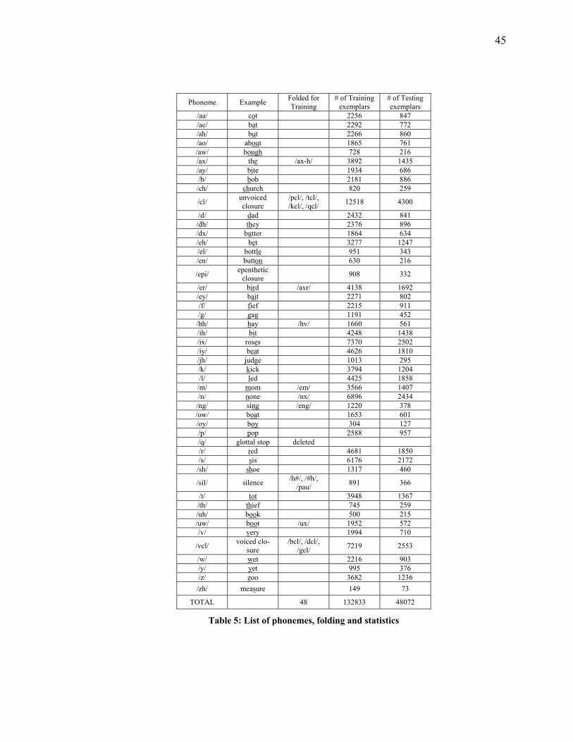
45
Phoneme Example Folded for Training
# of Training exemplars
# of Testing exemplars
/aa/ cot 2256 847 /ae/ bat 2292 772 /ah/ but 2266 860 /ao/ about 1865 761 /aw/ bough 728 216 /ax/ the /ax-h/ 3892 1435 /ay/ bite 1934 686 /b/ bob 2181 886 /ch/ church 820 259
/cl/ unvoiced closure
/pcl/, /tcl/, /kcl/, /qcl/ 12518 4300
/d/ dad 2432 841 /dh/ they 2376 896 /dx/ butter 1864 634 /eh/ bet 3277 1247 /el/ bottle 951 343 /en/ button 630 216
/epi/ epenthetic closure 908 332
/er/ bird /axr/ 4138 1692 /ey/ bait 2271 802 /f/ fief 2215 911 /g/ gag 1191 452
/hh/ hay /hv/ 1660 561 /ih/ bit 4248 1438 /ix/ roses 7370 2502 /iy/ beat 4626 1810 /jh/ judge 1013 295 /k/ kick 3794 1204 /l/ led 4425 1858 /m/ mom /em/ 3566 1407 /n/ none /nx/ 6896 2434
/ng/ sing /eng/ 1220 378 /ow/ boat 1653 601 /oy/ boy 304 127 /p/ pop 2588 957 /q/ glottal stop deleted /r/ red 4681 1850 /s/ sis 6176 2172 /sh/ shoe 1317 460
/sil/ silence /h#/, /#h/, /pau/ 891 366
/t/ tot 3948 1367 /th/ thief 745 259 /uh/ book 500 215 /uw/ boot /ux/ 1952 572 /v/ very 1994 710
/vcl/ voiced clo-sure
/bcl/, /dcl/, /gcl/ 7219 2553
/w/ wet 2216 903 /y/ yet 995 376 /z/ zoo 3682 1236
/zh/ measure 149 73
TOTAL 48 132833 48072
Table 5: List of phonemes, folding and statistics

46
During recognition, errors or confusions among the following phonemes were ig-
nored: {/sil/, /cl/, /vcl/, /epi/}, {/el/, /l/}, {/en/, /n/}, {/sh/, /zh/}, {/ao/, /aa/}, {/ih/, /ix/},
and {/ah/, /ax/}. Performing these foldings gives a total of 39 classes.
4.3 Time lags and embedding dimension
As described in section 3.1, Takens’ theorem gives the sufficient condition for the
size of the embedding, but does not specify a time lag. In practice, the determination of
the time lag can be difficult, because there is no theoretically well-founded method to as-
certain it, where an obvious criterion function can be formulated. Despite this caveat, two
heuristics have been developed in the literature for establishing a time lag: the first zero
of the autocorrelation function and the first minimum of the auto-mutual information
curve [8]. These heuristics are premised on the principle that it is desirable to have as lit-
tle information redundancy between the lagged versions of the time series as possible. If
the time lag is too small, the attractor structure will be compressed and the dynamics will
not be apparent. If the time lag is too large, the attractor will spread out immensely,
which also obscures the structure as evident from the figure below.
τ = 1 τ = 6 τ = 24τ = 1 τ = 6 τ = 24
Figure 15: Time lag comparison in RPS
Utilizing qualitative inspection of many phoneme attractors and by looking at the first
zero of the autocorrelation and first minimum of the auto-mutual information curves for

47
these phonemes, a time lag of 6 ( )6τ = was determined to be appropriate for all subse-
quent analysis [49]. This choice also is consistent with the results in [50] . A time lag of 6
is equal to 375 µs delay for data sampled at 16 kHz.
As explained previously, the proper embedding dimension must also be chosen to en-
sure accurate recovery of the dynamics, since the original dimension of the phase space
of speech phonemes is unknown. Again, there is no theoretically proven scheme for
discovering it, but a common heuristic known as false nearest neighbors is typically used
as explained in [8]. The false nearest neighbors algorithm calculates the percentage of
false crossings of the attractor as a function of the embedding dimension. False crossings
indicate that the attractor is not completely unfolded. The algorithm works by increasing
the dimension of the embedding until the percentage of false crossings drop below some
threshold.
Five hundred random phonemes were selected from the training partition of the cor-
pus. The false nearest neighbors algorithm given in [51] was executed on them using a
threshold of 0.1 % and a time lag of 6 ( )6τ = resulting in the histogram shown below.
Figure 16: False nearest neighbors for 500 random speech phonemes

48
The mode of this distribution is at an embedding dimension of 5 ( )5d = , and this was
the embedding dimension chosen. In addition, this choice is consistent with the results in
[23]. Incidentally, the ( )5,6,& fdnx and ( )5,6,&
n∆x actually constitute a 10 dimensional RPS, be-
cause the trajectory information is simply linear combinations of time delayed versions of
time series. For comparison, a ( )6d 10,τ= = feature vector, ( ),610nx was used as well.
The choice of time lag and embedding dimension are not independent. In practicality,
certain time lags will permit the attractor to unfold at a lower dimension than others. This
allows for a smaller embedding, which is advantageous for subsequent analysis. Further-
more, a RPS may be embedded at a dimension less than the sufficient condition of greater
than , if the dynamics of interest reside on a manifold of a lower dimension. Although
proper reconstruction of the dynamics is in general a relevant issue, the goal of this work
is to find a time lag and embedding dimension that yield favorable classification accuracy
in the final analysis.
2d
4.4 Number of mixtures
In order to determine how many mixtures are necessary to model the RPS derived
features, isolated phoneme classification experiments were performed. The feature vec-
tor, , described in section 3.2.1, was modeled using a one state HMM with a GMM
state distribution. Training was conducted using the training set for a particular number of
GMM mixtures, and then testing was performed over the testing set described in section
4.2. A classification experiment was carried out after each mixture increment and pa-
rameter retraining. The method employed to increment the number of mixtures was the
( )5,6nx

49
binary split scheme explained in section 2.2.1. The empirical classification accuracy can
then be plotted as a function of the number of mixtures as displayed below.
(%)
(%)
Figure 17: Classification accuracy vs. number of mixtures for RPS derived features Upon inspection of the graph, it is evident that the classification accuracy asymptotes at
approximately 128 mixtures, where the ‘elbow’ of the plot is located. If the number of
mixtures were further increased past 256 mixtures, test accuracy would at some point
drop due to overfitting. The number of mixtures was therefore set at 128 for all following
experimentation. A 128 mixture GMM appears to retain a balance between the complexi-
ties of the distribution of the RPS derived features and the overfitting issue elucidated in
section 2.2.1.
4.5 Baseline systems
Whenever a novel experimental system, especially in ASR, is designed, built, and
implemented, it must be compared to a baseline system. Ideally, the baseline system

50
should be the state-of-the-art system available at that time and the architecture of that sys-
tem should be well known in the research community at large. In this case, the baseline
system that is used for comparison was very similar to the one described in sections 1.1
and 2.3. This baseline system is familiar and frequently considered as the standard in
most of the literature [1-4], although it is not necessarily “state-of-the-art” in the sense
that it incorporates all known methods ever shown to boost accuracy.
A summary of the parameters used for MFCC feature computation is as follows: a
pre-emphasis coefficient of 0.97, a Hamming window with a size of 25 ms (400 time
samples), frame-speed/overlap size of 10 ms (160 time samples), and 24 triangular filter-
banks. It should be noted that these parameter choices are common. The precise HTK
configuration file can be found is the appendix. The model used was a one state HMM
with a GMM state distribution. The mixture number was set to 16 in all experiments us-
ing the MFCC features, which is quite typical. Mixture incrementing for these baseline
systems was executed by increasing the number of mixtures in the model by one. Follow-
ing this, incremental retraining was performed until 16 mixtures were reached.
4.6 Direct comparisons To test the performance of the classifier systems that use the RPS derived features
and the MFCC features, experiments were carried out using the respective feature vectors
alone. Performance is evaluated by simply examining the number of correct classifica-
tions each system achieved using the various features with their appropriate classifier sys-
tems lay out beforehand. The summary of the performance is displayed below. Confusion
matrix information on these experiments is given in appendix.

51
Feature set
Test set accuracy (48,072 total test ex-
emplars)
( )5,6nx 31.43 % (15017)
( )10,6nx 34.02 % (16353)
( )5,6,& fdnx
38.06 % (18296)
R
PS d
eriv
ed fe
atur
e se
ts (1
28
mix
ture
GM
M)
( )5,6,&n
∆x
39.19 % (18840)
tc
50.34 % (26372)
Bas
elin
e fe
a-tu
re se
ts
(16
mix
ture
G
MM
)
tO
54.86 % (24199)
Table 6: Direct performance comparison of the feature sets
As apparent from the table, the RPS derived feature sets attained approximately ~75
% the accuracy of the baseline, which translates into ~9182- 7532 more correct classifica-
tions for the baseline. Adding the extra 5 dimensions to ( )5,6nx , improved the accuracy by
~2.5 %. The appended RPS derived features that contained additional trajectory informa-
tion elements boost the x feature vector accuracy by more than ~7 %. ( )5,6n
4.7 Stream weights
In order to determine the correct stream weights to model the joint feature vector, ny ,
the testing accuracy was measured as a function of the stream weight, ρ , in equation
(3.3.2). The mixtures in the stream model 1 ( )1s = , which contained the RPS derived
features, were incremented using the binary split method, while the other stream model

52
( 2s = ) , which contained the MFCC feature set was incremented one mixture at a time
simultaneously with stream model 1. The stream model was initially trained up to the de-
sired number of mixtures, which was 1 2128, 16M M= = using 0.5ρ = . For all the other
values of ρ that were tested, ρ was varied and then retraining took place using the pa-
rameters from the 0.5ρ = model as the seed. Doing the training in this manner elimi-
nates the need to retrain each model from a flat start, since the mixture clusters are ap-
proximately in an acceptable location anyway [5]. As apparent from equation (3.3.2),
when 0ρ = , the model is essentially equivalent to the classifier system that uses ( )5,6,&n
∆x ,
and when 1ρ = , it is approximately equal to the MFCC feature set, O , except the
MFCCs were replicated according to equation (3.2.8). This makes the
t
1ρ = stream
model in effect on par as the baseline.
ρ
0.2 0.4 0.6ρ
Acc
urac
y (%
)
The plot of the testing accuracy versus is shown below.
0 0.8 135
40
45
50
55
60
65
Baseline
peak at 0.25
Figure 18: Accuracy vs. stream weight

53
As labeled in the figure, the peak of the plot is at 0.25ρ = . 4.8 Joint feature vector comparison
4.8.1 Accuracy results
The table below summarizes the comparisons made for values of ρ , the stream
weight.
ρ Test set accuracy (48,072 total test exemplars)
Peak value of joint feature vector 0.25 57.85 % (27810)
Baseline 1 55.04 % (26460)
Table 7: Comparisons for different stream weights
The higher accuracy was 57.85 % when 0.25ρ = . This ultimately results in a difference
of 1350 more training exemplars correctly classified by the joint feature beyond those of
the baseline.
4.8.2 Statistical tests
Two statistical tests were executed over the joint feature vector results on the
0.25ρ = and 1ρ =
5
classifiers. The first statistical test poses the question: Is the true er-
ror of 0.2ρ = classifier smaller then the error for the 1ρ = classifier under the as-
sumptions that the testing exemplars are independent and drawn from the same distribu-
tion as the training exemplars? Using the confidence interval methods described in [41,
42], the error is different to a significance level . 0 .99
The other statistical test poses the question: Which classifier will achieve better accu-
racy on a new set of testing exemplars drawn from the same task and problem domain

54
(e.g. performance on more hypothetical data collected identically in the manner in which
TIMIT was acquired, under the same conditions, equipment, etc.)? Using this test out-
lined in [42], the 0.25ρ = classifier will perform better than the 1ρ = classifier to a
significance level . 0 .99
4.9 Summary
This chapter presented the experimental framework and results for the isolated pho-
neme classification experiments that were run using both RPS derived features and base-
line MFCC features. The software and data (HTK and TIMIT) utilized are well known in
the community. The time lag, embedding dimension, mixture weights, and stream
weights were determined using empirical methods. Direct comparisons and joint feature
vector comparisons were made using overall accuracy, confusion matrices, and other sta-
tistical tests. The next chapter will interpret these results, draw conclusions, and propose
possible future work in this area.
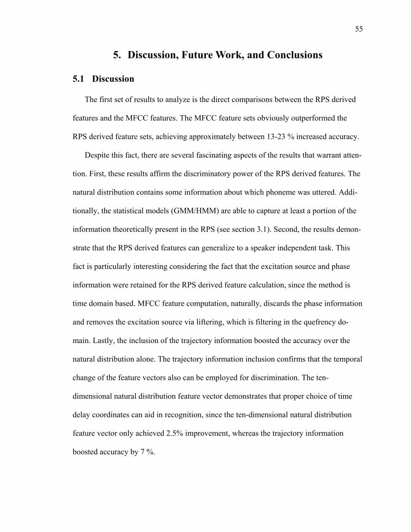
55
5. Discussion, Future Work, and Conclusions
5.1 Discussion
The first set of results to analyze is the direct comparisons between the RPS derived
features and the MFCC features. The MFCC feature sets obviously outperformed the
RPS derived feature sets, achieving approximately between 13-23 % increased accuracy.
Despite this fact, there are several fascinating aspects of the results that warrant atten-
tion. First, these results affirm the discriminatory power of the RPS derived features. The
natural distribution contains some information about which phoneme was uttered. Addi-
tionally, the statistical models (GMM/HMM) are able to capture at least a portion of the
information theoretically present in the RPS (see section 3.1). Second, the results demon-
strate that the RPS derived features can generalize to a speaker independent task. This
fact is particularly interesting considering the fact that the excitation source and phase
information were retained for the RPS derived feature calculation, since the method is
time domain based. MFCC feature computation, naturally, discards the phase information
and removes the excitation source via liftering, which is filtering in the quefrency do-
main. Lastly, the inclusion of the trajectory information boosted the accuracy over the
natural distribution alone. The trajectory information inclusion confirms that the temporal
change of the feature vectors also can be employed for discrimination. The ten-
dimensional natural distribution feature vector demonstrates that proper choice of time
delay coordinates can aid in recognition, since the ten-dimensional natural distribution
feature vector only achieved 2.5% improvement, whereas the trajectory information
boosted accuracy by 7 %.

56
The results obtained from the joint feature vector provide insight into the information
content of it. The 0.25ρ = classifier attained a 2.81 % increase in accuracy over
the 1ρ = system (baseline). This result suggests that the RPS derived features contain
discriminatory information not present in the MFCC features, otherwise the result would
have been the same or lower. The statistical tests further affirm these results by providing
knowledge about the bounds on the error and the expected performance of the classifiers
on more testing data.
Another interesting characteristic of these results is the shape of the curve. The curve
implies that as soon as RPS derived features are incorporated, the accuracy increases over
the baseline. This fact, along with where the peak accuracy occurs, shows that additional
information, beyond that contained in the MFCC features, is actually present, but that it
needs to be combined in an intelligent way.
5.2 Known issues and future work
5.2.1 Feature extraction
There are two main but related issues that arise when computing the RPS derived fea-
tures: amplitude scaling and the absence of an energy measure. Due to the nature of the
technique, the features are based in the time domain, and therefore, the dynamic range of
the time series affects the range of the data in the RPS. The dynamic range or amplitude
of the signal is known to be irrelevant to the classification process, because the amplitude
is affected by experimental nuances such as the distance the speaker is from the micro-
phone during data collection. One advantage of the MFCC features is that they are totally
invariant to this issue, because the energy is normalized out on a frame-by-frame basis. In
the case of the RPS derived features though, the problem is partially solved by using the

57
normalization procedure described in section 3.2, but future work could include discover-
ing a robust method to make this approach independent of amplitude scaling effects. This
issue is of particular concern when performing continuous recognition, because there is
no way to normalize the data on a phoneme-by-phoneme basis, since the time boundary
information would not be present. This concern seriously hampers effective implementa-
tion for a continuous speech task.
The other related issue is that of computing an energy measure. Again, the MFCC
features incorporate an energy measure by computing it for each frame, given in equation
(2.1.10). For the proposed RPS derived features though, there is no analysis window, and
therefore, no way to compute a meaningful energy measure that can be incorporated di-
rectly into the feature vector. One method would be to compute the energy over an entire
phoneme, and then replicate it for each feature vector. But, once again, for continuous
recognition, phoneme boundaries are unknown, and computing such a measure may be
difficult. To reiterate then, both of these issues must be addressed in order for the RPS
derived features to have long-term success for speech recognition applications.
Another notion that warrants further study is whether a higher dimensional RPS
would improve classification accuracy. All of the experiments presented here utilized a
five and ten dimensional RPS, whereas a larger dimensional RPS could further expand
out the characteristic attractor structure. The premise is that a larger dimensional RPS
may produce bigger differences between phoneme attractors that would have been per-
haps overlapping in a smaller dimensional RPS. Further experimentation could be per-
formed on time lags as well especially on how they relate to speaker variability.

58
All of the methods presented here can be applied to any arbitrary time series that has
originated from a dynamical system. Investigation into the implementation of speech
models, similar to the source-filter model employed in the linear regime, but applied to
the RPS may produce valuable results. Also, features could be extracted from a frame
that uses a RPS as processing space such as higher-order statistical moments. Such a fea-
ture set could be integrated into the existing frame based ASR systems with relative ease.
5.2.2 Pattern recognition
In addition to modifications that could be made in the feature extraction process, spe-
cific pattern recognition improvements could be employed to further expand the methods.
One such method would be the implementation of a fully connected HMM. By substitut-
ing the simple one state HMM model (128 mixture GMM state distribution), with a 128
state HMM (single mixture GMM state distribution), the trajectory information could be
captured through the convenient statistical framework of the transition probabilities. The
transition probability parameters would represent the probability of attractor moving from
one neighborhood of the RPS to another. The initial experimentation into this approach
found that the method can be effective, but the computational cost is very high, because
the model is complex. The computation time of such an approach would have to be re-
duced to make the method feasible. Also on the topic of trajectory, higher-order trajec-
tory information such as delta-deltas could boost accuracy similar to the result of the first
delta presented here.
The method of data fusion or classifier combination implemented was a stream
model. Although this method is well founded, it is rather naïve and does not necessarily

59
do the best job of unifying the knowledge extracted from radically different processing
spaces. An improved method of fusing the data would be desirable.
5.2.3 Continuous speech recognition
In addition to the isolated phoneme classification experiments presented and de-
scribed here, the task of continuous speech recognition using the RPS derived features
was examined. Above and beyond the issues of amplitude scaling and energy measure
calculation, there is another difficulty that occurs when attempting to employ the RPS
derived features for a continuous speech recognition task. The issue is state duration. Im-
plicit to the approach of the MFCC features is the use of an analysis window, which
automatically enforces a duration during continuous speech recognition; the fastest transi-
tion that the recognizer can make is ~10 ms, since that is the speed at which the feature
vector changes in time. A ~10 ms speed generally coincides with the amount of time that
any particular speech phoneme is stationary and relates to the rate at which phonemes
change in time. This implicit duration then makes the classic left-to-right HMM with
constant self-transition probabilities functional. In case of the RPS derived features,
though, the feature vector changes on a time sample-by-time sample basis, and therefore
this implicit duration that is present in the MFCC features no longer exists. Some resolu-
tion to the issue of state duration must be instituted in order for the RPS derived features
to have ultimate success in the future for continuous speech recognition applications.
5.3 Conclusions
This thesis has presented a novel technique for speech recognition using features ex-
tracted from phase space reconstructions. The methods have a sound theoretical justifica-
tion provided by the nonlinear dynamics literature. The specific approach transfers the

60
analytical focus from the frequency domain to the time domain, which presents a radi-
cally unique way of viewing the speech recognition problem and offers an opportunity to
capture the nonlinear dynamical information present in the speech production mecha-
nism. The features derived from the RPS are created using the natural distribution and
trajectory information of phoneme attractors. By using statistical models (GMM/HMM),
the salient information contained in the RPS derived features can be captured for subse-
quent classification.
The experiments that were run affirm the discriminatory power of the RPS derived
features. The direct comparisons demonstrated the potential of these features for speech
recognition applications. The joint feature vector results imply that the information con-
tent between the RPS derived features and the MFCC feature sets are not identical, be-
cause the accuracy was boosted over the baseline.
As a direct outcome of this work, several possible future research avenues were dis-
covered in conjunction with issues that are inherent to the method. Questions of ampli-
tude scaling, energy measures, better modeling techniques, and state duration present a
number of interesting areas of continued investigation.
Overall, this work deviates strongly from mainstream research in speech recognition.
This research has extended the fundamental understanding of the speech recognition
problem and simultaneously expanded the knowledge of the nonlinear techniques pre-
sented for classification applications. In conclusion, reconstructed phase space analysis is
an attractive research avenue for increasing speech recognition accuracy as demonstrated
through the results, and future work will determine its overall feasibility and long-term
success for both isolated and continuous speech recognition applications.

61
6. Bibliography and References
[1] B. Gold and N. Morgan, Speech and Audio Signal Processing. New York: John Wiley & Sons Inc., 2000.
[2] J. R. Deller, J. H. L. Hansen, and J. G. Proakis, Discrete-Time Processing of Speech Signals, vol. IEEE Press, Second ed. New York, 2000.
[3] C. Becchetti and L. P. Ricotti, Speech Recognition. Chichester: John Wiley & Sons, Inc., 1999.
[4] F. Jelinek, Statistical Methods for Speech Recognition. Cambridge: The MIT Press, 1997.
[5] S. Young, G. Evermann, D. Kershaw, G. Moore, J. Odell, D. Ollason, V. Valtchev, and P. Woodland, The HTK Book: Microsoft Corporation, 2001.
[6] T. Sauer, J. A. Yorke, and M. Casdagli, "Embedology," Journal of Statistical Physics, vol. 65, pp. 579-616, 1991.
[7] F. Takens, "Dynamical systems and turbulence," in Lecture Notes in Mathemat-ics, vol. 898, D. A. Rand and L. S. Young, Eds. Berlin: Springer, 1981, pp. 366-81.
[8] H. D. I. Abarbanel, Analysis of Observed Chaotic Data, softcover ed. New York: Springer-Verlag, 1996.
[9] H. Kantz and T. Schreiber, Nonlinear Time Series Analysis, vol. 7, Paperback ed. Cambridge: Cambridge University Press, 1997.
[10] A. V. Oppenheim, R. W. Shafer, and J. R. Buck, Discrete-Time Signal Process-ing, second ed. Upper Saddle River: Prentice Hall, 1999.
[11] W. V. d. Water and J. D. Weger, "Failure of chaos control," Physical Review E, vol. 62, pp. 6398-408, 2000.

62
[12] A. C. Lindgren, M. T. Johnson, and R. J. Povinelli, "Speech recognition using phase space features," presented at IEEE International Conference on Acoustics, Speech, and Signal Processing, Hong Kong, China, 2003.
[13] M. T. Johnson, A. C. Lindgren, R. J. Povinelli, and X. Yuan, "Performance of nonlinear speech enhancement using phase space reconstruction," presented at IEEE International Conference on Acoustics, Speech, and Signal Processing, Hong Kong, China, 2003.
[14] A. Petry, D. Augusto, and C. Barone, "Speaker Identification using nonlinear dy-namical features," Chaos, Solitons, and Fractals, vol. 13, pp. 221-231, 2002.
[15] V. Pitsikalis and P. Maragos, "Speech analysis and feature extraction using cha-otic models," presented at EEE International Conference on Acoustics, Speech, and Signal Processing, Orlando, Florida, 2002.
[16] R. J. Povinelli, J. F. Bangura, N. A. O. Demerdash, and R. H. Brown, "Diagnos-tics of bar and end-ring connector breakage faults in polyphase induction motors through a novel dual track of time-series data mining and time-stepping coupled FE-state space modeling," IEEE Transactions on Energy Conversion, vol. 17, pp. 39-46, 2002.
[17] F. M. Roberts, R. J. Povinelli, and K. M. Ropella, "Identification of ECG ar-rhythmias using phase space reconstruction," presented at Principles and Practice of Knowledge Discovery in Databases (PKDD'01), Freiburg, Germany, 2001.
[18] D. M. Tumey, P. E. Morton, D. F. Ingle, C. W. Downey, and J. H. Schnurer, "Neural network classification of EEG using chaotic preprocessing and phase space reconstruction," presented at IEEE Seventh Annual Northeast Bioengineer-ing Conference, 1991.
[19] L. I. Eguiluz, M. Manana, and J. C. Lavandero, "Disturbance classification based on the geometrical properties of signal phase space representation," presented at International Conference on Power System Technology, 2000.
[20] Y. C. Lai, Y. Nagai, and C. Grebogi, "Characterization of natural measure by un-stable periodic orbits in chaotic attractors," Physical Review Letters, vol. 79, pp. 649-52, 1997.

63
[21] C. Grebogi, E. Ott, and J. A. Yorke, "Unstable periodic orbits and the dimensions of multifractal chaotic attractors," Physical Review A, vol. 37, pp. 1711-24, 1988.
[22] E. Ott, Chaos in Dynamical Systems. Cambridge: Cambridge University Press, 1993.
[23] M. Banbrook, S. McLaughlin, and I. Mann, "Speech characterization and synthe-sis by nonlinear methods," IEEE Transactions on Speech and Audio Processing, vol. 7, pp. 1-17, 1999.
[24] R. Hegger, H. Kantz, and L. Matassini, "Denoising human speech signals using chaoslike features," Physical Review Letters, vol. 84, pp. 3197-3200, 2000.
[25] R. Hegger, H. Kantz, and L. Matassini, "Noise reduction for human speech sig-nals by local projections in embedding spaces," IEEE Transactions on Circuits and Systems - I: Fundamental Theory and Applications, vol. 48, pp. 1454-1461, 2001.
[26] G. Kubin, "Nonlinear speech processing," in Speech Coding and Synthesis, W. B. Kleijn and K. K. Paliwal, Eds.: Elsevier Science, 1995.
[27] A. Kumar and S. K. Mullick, "Nonlinear dynamical analysis of speech," Journal of the Acoustical Society of America, vol. 100, pp. 615-629, 1996.
[28] A. Langi and W. Kinsner, "Consonant characterization using correlation fractal dimension for speech recognition," presented at IEEE WESCANEX, 1995.
[29] C. Liang, C. Yanxin, and Z. Xiongwei, "Research on speech recognition on phase space reconstruction theory," presented at Advances in Multimodal Interfaces-ICMI 2000, Berlin, Germany, 2000.
[30] I. Mann and S. McLaughlin, "Synthesizing natural sounding vowels using a nonlinear dynamical model," Signal Processing, vol. 81, pp. 1743-56, 2001.
[31] S. S. Narayanan and A. A. Alwan, "A nonlinear dynamical systems analysis of fricative consonants," Journal of the Acoustical Society of America, vol. 97, pp. 2511-2524, 1995.

64
[32] W. Rodriguez, H.-N. Teodorescu, F. Grigoras, A. Kandel, and H. Bunkell, "A fuzzy information space approach to speech signal nonlinear analysis," Interna-tional Journal of Intelligent Systems, vol. 15, pp. 343-363, 2000.
[33] S. Sabanal and M. Nakagawa, "The fractal properties of vocal sounds and their application in the speech recognition model," Chaos, Solitons, & Fractals, vol. 7, pp. 1825-1843, 1996.
[34] N. Tishby, "A dynamical systems approach to speech processing," presented at IEEE International Conference on Acoustics, Speech, and Signal Processing, Al-buquerque, New Mexico, 1990.
[35] E. Kostelich and T. Schreiber, "Noise reduction in chaotic time series: a survey of common methods," Physical Review E, vol. 48, pp. 1752-1763, 1993.
[36] I. T. Nabney, NETLAB: Algorithms for Pattern Recognition. London: Springer, 2001.
[37] R. O. Duda, P. E. Hart, and D. G. Stork, Pattern Classification, Second ed. New York: John Wiley & Sons, Inc., 2001.
[38] A. P. Dempster, N. M. Laird, and D. B. Rubin, "Maximium likelihood from in-complete data via the EM algorithm," Journal of the Royal Statistical Society, Se-ries B, vol. 39, pp. 1-38, 1977.
[39] A. Papoulis and A. U. Pillai, Probability, Random Variables, and Stochastic Processes, Fourth ed. Boston: McGraw Hill, 2002.
[40] L. R. Rabiner, "A tutorial on Hidden Markov Models and selected application in speech recognition," Proceedings of the IEEE, vol. 77, pp. 257-286, 1989.
[41] T. M. Mitchell, Machine Learning. Boston: McGraw-Hill, 1997.
[42] A. Webb, Statistical Pattern Recognition. London: Arnold Publishing, 1999.
[43] H. Whitney, "Differentiable manifolds," The Annals of Mathematics, 2nd Series, vol. 37, pp. 645-680, 1936.

65
[44] N. H. Packard, J. P. Crutchfield, J. D. Farmer, and R. S. Shaw, "Geometry from a time series," Physical Review Letters, vol. 45, pp. 712-716, 1980.
[45] P. Blanchard, R. L. Devaney, and G. R. Hall, Differential Equations. Pacific Grove: Brooks/Cole Publishing Company, 1998.
[46] "MATLAB," 6.2 ed: The MathWorks Inc., 2003.
[47] J. Garofolo, L. Lamel, W. Fisher, J. Fiscus, D. Pallet, N. Dahlgren, and V. Zue, "TIMIT Acoustic-Phonetic Continuous Speech Corpus," Linguistic Data Consor-tium 1993.
[48] K. F. Lee and H. W. Hon, "Speaker-independent phone recognition using Hidden Markov Models," IEEE Transactions on Acoustics, Speech, and Signal Process-ing, vol. 37, pp. 1641-1648, 1989.
[49] C. Merkwirth, U. Parlitz, I. Wedekind, and W. Lauterborn, "TS Tools," http://www.physik3.gwdg.de/tstool/index.html, 2001.
[50] M. A. Jackson and I. S. Burnett, "Phase-space portraits of speech employing mu-tual information and perceptual masking," presented at IEEE Workshop on Speech Coding: Models, Coders, and Error Criteria, 1999.
[51] R. Hegger, H. Kantz, and T. Schreiber, "Practical implementation of nonlinear time series methods: The TISEAN Package," Chaos, vol. 413, pp. 413-435, 1999.

66
Appendix A – Confusion Matrices
In addition to inspection of the raw accuracy numbers (e.g. # of correct classifica-
tions/# of attempted classifications), other, more detailed results can be compiled, which
give supplementary information on the performance of the classifier system. On such rep-
resentation that reveals the specific classification errors or class confusions is a confusion
matrix.
A confusion matrix is formed by creating rows and columns for each class in the set.
The rows represent the expert labels or true classes of the testing exemplars, while the
columns correspond to the classifier system’s output or it’s hypothesized class label. The
confusions are then tabulated and inserted into the correct position in the matrix. For ex-
ample, looking at the table below, the phoneme ‘/p/’ was classified correctly twelve
times, and classified as ‘/r/’ twice, ‘/s/’ once, and ‘/sh/’ never. It is clear therefore, that
the main diagonal of the matrix, displayed in table form, are the correct classifications,
while the off-diagonal elements are the errors. Consequently, the confusion matrix un-
covers correlated errors and further illustrates how a classifier is performing on each class
individually. The confusion matrices present here were generated automatically using
HTK.
/p/ /r/ /s/ /sh/ /p/ 12 2 1 0 /r/ 4 24 6 1 /s/ 0 1 32 5
/sh/ 0 3 7 21
Table 8: Example of a confusion matrix
Note: The notation for the various feature vectors labeled in following confusion matrices
is given in Chapter 4.

67
------------------------ Overall Results -------------------------- SENT: %Correct=31.24 [H=15017, S=33055, N=48072] WORD: %Corr=31.24, Acc=31.24 [H=15017, D=0, S=33055, I=0, N=48072] ------------------------ Confusion Matrix ------------------------- d j c s s z f t v d m n e r w y h e i i e e a a a a a o o u u e s d k g t b p x h h h h h g n h l y h h y e w y h o y w h w r i l Del [ %c / %e] dx 103 1 0 1 6 3 0 0 81 24 32 13 32 6 11 26 12 3 35 24 10 22 2 0 1 8 1 1 0 11 30 21 72 1 4 8 1 27 1 0 [16.2/1.1] jh 3 8 26 33 65 22 6 6 0 15 0 0 1 0 1 3 9 0 0 0 0 0 0 0 0 0 0 0 0 0 0 0 20 31 21 4 16 3 2 0 [ 2.7/0.6] ch 1 2 54 43 40 20 1 10 0 10 0 0 1 0 0 0 3 0 0 0 0 0 0 0 0 0 0 0 0 0 0 0 20 16 15 0 21 1 1 0 [20.8/0.4] s 0 50 245 744 552 244 39 28 0 6 0 0 0 0 0 0 9 1 0 0 0 0 2 2 0 1 2 1 1 0 1 0 76 15 115 0 29 3 6 0 [34.3/3.0] sh 2 4 44 128 216 33 4 5 0 18 0 0 0 0 0 1 15 0 0 0 0 0 1 0 0 0 0 0 0 0 1 0 22 16 16 1 1 5 0 0 [40.5/0.7] z 6 18 83 191 469 200 22 13 0 14 0 0 1 0 0 4 19 0 1 3 0 0 2 1 2 2 1 0 0 0 11 0 56 14 80 6 15 1 1 0 [16.2/2.2] f 0 4 27 57 158 149 260 14 2 1 0 0 0 0 0 0 39 0 0 0 0 0 0 0 0 0 0 0 0 0 0 0 105 3 66 4 8 0 14 0 [28.5/1.4] th 0 2 8 5 40 16 19 24 0 2 0 0 1 0 0 0 10 0 0 0 0 1 0 0 0 0 0 0 0 0 0 0 100 6 13 3 2 5 2 0 [ 9.3/0.5] v 52 1 4 1 17 1 10 1 235 27 22 21 44 4 22 22 44 12 13 7 0 2 0 1 0 9 0 0 0 1 19 7 98 0 9 1 0 3 0 0 [33.1/1.0] dh 75 0 5 2 19 2 11 13 58 54 20 15 65 1 4 27 31 0 23 24 1 6 0 0 1 4 0 0 0 5 30 6 181 51 14 23 5 109 11 0 [ 6.0/1.8] m 59 0 0 1 10 0 0 0 81 8 420 106 360 3 7 62 25 5 54 17 1 0 2 0 1 11 1 0 0 0 14 2 149 1 0 1 0 6 0 0 [29.9/2.1] ng 10 0 0 0 1 0 0 0 18 5 25 90 107 0 2 23 3 4 30 17 3 1 0 0 1 1 0 0 0 2 11 1 21 0 0 0 0 2 0 0 [23.8/0.6] en 81 0 0 1 9 1 0 0 122 27 289 409 881 14 8 113 33 10 149 71 11 10 10 7 1 38 2 4 1 5 54 24 243 3 2 5 0 11 1 0 [33.2/3.7] r 31 0 0 1 7 2 1 0 41 1 1 14 5 162 40 26 19 57 38 87 123 86 79 72 58 148 170 20 41 91 80 312 9 0 9 7 1 10 1 0 [ 8.8/3.5] w 23 0 0 0 3 0 0 0 24 3 4 13 2 7 235 16 7 129 60 47 10 35 11 5 4 16 57 23 6 45 75 9 7 0 0 0 0 27 0 0 [26.0/1.4] y 15 0 0 0 0 0 0 0 6 5 17 25 45 2 4 99 4 1 79 17 0 13 0 0 0 0 0 0 0 5 25 0 11 0 0 1 1 1 0 0 [26.3/0.6] hh 2 0 6 35 50 32 50 0 24 14 5 17 32 0 1 8 164 2 11 3 0 1 2 3 1 5 2 0 0 0 5 0 57 0 24 1 1 0 3 0 [29.2/0.8] el 37 0 0 0 2 0 0 1 44 7 13 42 20 24 154 24 17 446 89 136 79 113 59 52 51 92 298 72 20 133 110 39 14 1 1 0 0 11 0 0 [20.3/3.7] iy 59 0 0 0 2 0 0 0 31 11 22 98 122 5 35 280 2 5 616 168 7 111 2 0 0 12 0 0 0 11 181 6 18 1 0 0 0 5 0 0 [34.0/2.5] ih 106 0 0 0 12 1 0 1 106 27 9 134 61 52 55 105 15 27 438 810 187 546 63 8 3 188 1 8 13 284 471 165 9 3 1 7 0 24 0 0 [20.6/6.5] eh 1 0 0 0 0 0 0 0 6 0 0 5 0 42 5 0 6 11 8 51 364 210 173 24 14 129 22 15 21 73 5 58 1 0 2 0 1 0 0 0 [29.2/1.8] ey 5 0 0 0 0 0 0 1 9 0 0 10 0 11 11 0 3 10 68 83 92 360 37 3 2 26 0 1 1 27 20 15 0 0 0 0 0 7 0 0 [44.9/0.9] ae 1 0 0 0 3 0 0 0 4 1 0 4 0 4 1 0 9 7 0 15 129 51 294 82 42 56 62 1 3 1 0 0 0 0 1 0 1 0 0 0 [38.1/1.0] aw 0 0 1 1 1 0 0 0 0 0 0 0 0 1 0 0 1 1 0 0 7 2 22 48 24 17 86 0 1 1 0 0 1 0 1 0 0 0 0 0 [22.2/0.3] ay 0 0 0 2 0 3 1 0 0 0 0 0 0 1 0 0 8 3 0 0 27 9 88 120 140 81 186 3 7 1 0 1 1 0 3 0 0 1 0 0 [20.4/1.1] ah 22 1 4 5 24 6 1 0 46 11 3 34 23 57 30 13 33 82 49 183 233 151 175 90 61 303 168 33 51 157 77 108 24 2 12 4 1 18 0 0 [13.2/4.1] ao 0 0 0 5 3 1 0 0 1 0 0 0 0 10 7 0 9 122 0 3 24 5 78 169 78 79 910 50 16 21 2 5 1 0 8 1 0 0 0 0 [56.6/1.5] oy 0 0 0 0 0 0 0 0 0 0 0 0 0 5 2 0 1 14 0 0 18 3 6 4 2 12 14 30 4 7 0 4 0 0 1 0 0 0 0 0 [23.6/0.2] ow 0 0 0 0 1 0 0 0 0 1 0 1 0 20 14 0 3 97 1 8 67 52 35 24 12 42 77 49 25 48 4 17 0 0 1 0 0 1 1 0 [ 4.2/1.2] uh 4 0 0 0 0 0 0 0 0 0 0 1 0 5 2 0 0 12 8 24 9 25 0 0 0 9 7 2 4 50 32 19 0 0 1 0 0 1 0 0 [23.3/0.3] uw 12 0 0 0 4 0 0 0 5 0 6 13 28 3 11 82 0 4 104 58 4 11 0 0 0 10 0 2 0 27 172 12 3 0 0 0 0 1 0 0 [30.1/0.8] er 42 0 0 0 8 0 0 0 49 6 0 16 3 114 28 4 9 32 28 155 85 107 55 35 14 86 32 26 27 167 92 432 8 2 7 15 0 8 0 0 [25.5/2.6] sil 104 1 33 60 366 96 178 46 169 186 130 18 268 1 4 70 490 3 28 22 1 3 5 3 1 3 1 1 0 0 18 3 4806 22 288 48 20 40 15 0 [63.6/5.7] d 58 1 9 11 67 14 11 8 12 29 3 3 14 2 3 8 48 3 8 21 0 4 2 0 1 7 0 2 1 2 11 5 39 152 38 48 19 164 13 0 [18.1/1.4] k 4 2 16 31 55 31 57 31 9 40 0 0 0 0 1 0 57 2 0 0 0 0 1 2 1 1 4 1 0 0 0 0 106 102 431 115 36 25 43 0 [35.8/1.6] g 25 0 1 5 12 4 4 3 7 33 1 2 11 2 8 17 12 2 6 2 0 1 0 0 0 1 2 0 0 1 3 2 32 39 50 114 7 38 5 0 [25.2/0.7] t 3 12 70 72 149 82 80 34 2 24 0 0 4 1 0 0 68 0 0 0 0 0 2 0 1 1 1 0 0 0 0 0 104 141 214 62 162 31 47 0 [11.9/2.5] b 52 0 0 5 19 1 3 11 41 39 13 10 27 9 15 17 22 13 6 20 4 8 0 0 3 12 3 0 2 13 11 7 80 68 14 21 1 306 10 0 [34.5/1.2] p 4 4 11 69 49 44 101 40 12 31 1 0 1 1 1 2 80 0 0 0 0 0 2 2 1 3 2 0 0 1 0 1 83 54 127 46 27 60 97 0 [10.1/1.8] Ins 0 0 0 0 0 0 0 0 0 0 0 0 0 0 0 0 0 0 0 0 0 0 0 0 0 0 0 0 0 0 0 0 0 0 0 0 0 0 0 ===================================================================
Table 9: Confusion matrix for ( )5,6nx
------------------------ Overall Results -------------------------- SENT: %Correct=34.02 [H=16353, S=31718, N=48071] WORD: %Corr=34.02, Acc=34.02 [H=16353, D=0, S=31718, I=0, N=48071] ------------------------ Confusion Matrix ------------------------- d j c s s z f t v d m n e r w y h e i i e e a a a a a o o u u e s d k g t b p x h h h h h g n h l y h h y e w y h o y w h w r i l Del [ %c / %e] dx 141 1 0 0 5 2 0 0 65 33 42 7 26 10 10 26 9 8 17 45 12 12 3 0 0 6 0 0 2 13 30 18 57 7 4 8 0 15 0 0 [22.2/1.0] jh 2 24 25 34 71 15 3 7 0 10 0 0 1 0 0 0 3 0 0 0 0 0 0 0 0 0 0 0 0 0 0 0 16 27 27 3 23 1 3 0 [ 8.1/0.6] ch 0 13 62 47 44 6 6 10 0 5 0 0 0 0 0 0 0 0 0 0 0 0 0 0 0 0 0 0 0 0 0 0 11 7 16 0 31 0 1 0 [23.9/0.4] s 0 50 250 933 443 131 65 34 0 1 0 0 0 0 0 0 8 0 0 0 0 0 0 0 0 0 0 0 0 0 1 0 56 6 158 3 25 5 3 0 [43.0/2.6] sh 0 13 47 136 226 22 2 9 0 6 0 0 0 0 0 0 7 0 0 0 0 0 0 0 0 0 0 0 0 0 1 0 17 8 31 1 1 6 0 0 [42.4/0.6] z 5 33 98 225 421 169 32 19 1 7 0 0 1 0 0 5 15 0 1 2 0 0 1 0 0 0 0 0 0 0 6 0 30 13 113 11 21 3 4 0 [13.7/2.2] f 0 7 33 151 85 38 347 24 0 1 0 0 0 0 0 0 20 0 0 0 0 0 0 0 0 0 0 0 0 0 0 0 99 4 49 2 27 1 23 0 [38.1/1.2] th 0 4 8 13 36 6 23 44 0 5 0 0 1 0 0 0 8 0 0 0 0 0 0 0 0 0 0 0 0 0 0 0 72 5 11 4 11 3 5 0 [17.0/0.4] v 34 0 4 3 12 2 10 1 290 31 27 22 38 0 16 23 39 5 2 15 0 1 0 1 0 7 0 0 1 4 14 6 80 2 8 1 3 4 4 0 [40.8/0.9] dh 64 2 5 2 20 0 15 20 69 84 27 15 56 0 3 26 21 0 12 29 3 3 0 0 0 9 0 0 0 9 32 4 130 72 18 34 7 87 18 0 [ 9.4/1.7] m 35 0 0 0 8 1 0 0 64 13 551 120 327 0 5 73 14 2 32 12 0 0 1 1 0 8 1 0 0 0 25 1 112 0 0 0 0 1 0 0 [39.2/1.8] ng 5 0 0 0 1 0 0 0 20 6 39 93 100 0 8 17 3 4 16 23 1 1 0 0 0 1 1 1 0 1 19 1 17 0 0 0 0 0 0 0 [24.6/0.6] en 52 0 0 0 6 0 0 1 129 27 513 408 795 4 21 104 28 11 97 84 5 7 11 7 0 34 0 0 1 4 88 27 166 5 3 6 0 5 1 0 [30.0/3.9] r 19 0 0 3 6 4 0 0 37 2 1 12 7 160 44 20 6 58 26 104 112 73 67 79 44 196 119 31 74 99 110 313 1 3 4 3 0 12 1 0 [ 8.6/3.5] w 18 0 0 1 3 0 2 0 17 7 1 12 5 3 299 22 3 119 18 48 10 21 12 5 3 17 48 29 20 45 96 7 1 1 0 0 0 10 0 0 [33.1/1.3] y 12 0 0 0 0 0 0 0 6 5 29 19 38 1 2 102 4 1 40 30 0 7 0 0 0 2 0 0 0 5 62 0 8 1 0 0 1 1 0 0 [27.1/0.6] hh 3 0 7 38 38 2 38 3 15 6 4 10 22 0 0 6 216 1 3 9 0 1 3 4 0 5 0 1 0 0 9 0 60 1 35 0 5 1 15 0 [38.5/0.7] el 20 0 0 1 0 0 0 1 28 8 19 33 20 19 151 32 15 466 44 170 69 60 47 59 21 129 282 59 91 145 150 46 5 0 1 1 2 7 0 0 [21.2/3.6] iy 40 0 0 0 2 0 0 0 38 9 46 102 67 6 44 293 5 2 344 244 9 83 3 0 0 16 0 0 0 37 404 8 4 1 0 0 0 3 0 0 [19.0/3.0] ih 53 0 0 0 16 0 0 0 100 22 12 131 55 24 58 73 19 31 1441022 213 300 61 8 1 229 1 17 27 501 571 218 3 5 1 3 1 20 0 0 [25.9/6.1] eh 1 0 0 0 0 0 0 0 2 0 0 3 0 23 4 1 7 14 0 52 407 122 184 23 12 170 14 20 37 82 5 62 0 0 2 0 0 0 0 0 [32.6/1.7] ey 4 0 0 0 0 0 0 1 5 0 0 4 0 11 21 1 4 14 8 119 117 275 39 3 0 41 0 5 15 59 34 18 0 0 0 0 0 4 0 0 [34.3/1.1] ae 1 0 0 1 0 0 0 0 3 0 0 2 0 5 0 1 9 10 0 20 116 11 336 78 57 70 38 2 2 1 0 2 0 2 2 0 0 3 0 0 [43.5/0.9] aw 0 0 0 1 0 1 0 0 0 0 0 0 0 1 0 0 1 1 0 0 6 0 21 57 43 18 62 0 1 1 0 0 0 0 2 0 0 0 0 0 [26.4/0.3] ay 0 0 0 0 0 4 0 0 0 0 0 0 0 1 0 0 5 1 1 0 27 6 96 110 219 81 122 1 5 1 0 1 0 0 5 0 0 0 0 0 [31.9/1.0] ah 14 1 2 9 15 5 1 0 36 15 1 39 24 34 22 9 34 55 12 224 234 102 164 94 41 413 139 34 102 162 77 121 23 4 12 7 1 12 1 0 [18.0/3.9] ao 0 0 0 4 0 2 0 0 1 0 0 0 0 12 10 0 10 134 0 4 22 2 98 179 90 96 839 43 33 17 2 2 0 0 6 2 0 0 0 0 [52.2/1.6] oy 0 0 0 0 0 0 0 0 1 0 0 0 0 4 3 0 0 11 0 1 14 2 10 2 2 9 11 39 11 5 0 2 0 0 0 0 0 0 0 0 [30.7/0.2] ow 0 0 0 0 0 0 1 0 0 0 0 1 0 13 6 0 2 80 1 7 69 44 23 17 5 65 71 48 75 48 3 21 0 0 1 0 0 0 0 0 [12.5/1.1] uh 1 0 0 0 0 0 0 0 0 1 0 0 0 3 0 0 0 11 3 27 8 19 0 0 0 10 4 3 8 63 32 22 0 0 0 0 0 0 0 0 [29.3/0.3] uw 3 0 0 0 1 0 0 0 4 2 13 13 14 1 14 87 2 3 56 60 2 6 1 0 0 6 0 2 2 44 222 12 0 0 0 1 0 1 0 0 [38.8/0.7] er 29 0 0 0 4 2 0 0 42 10 0 8 4 102 20 8 6 30 14 207 91 79 36 35 6 117 16 27 56 159 86 476 3 1 4 8 0 6 0 0 [28.1/2.5] sil 102 14 32 91 412 29 314 73 120 208 174 17 159 1 10 72 197 4 17 15 0 2 6 1 1 4 0 1 0 3 15 1 4934 34 266 78 45 21 78 0 [65.3/5.4] d 28 9 4 7 56 8 16 4 7 36 4 4 9 1 3 12 28 0 6 19 0 3 1 1 1 8 0 2 1 1 10 6 36 231 40 64 27 125 22 0 [27.5/1.3] k 0 11 17 25 45 8 50 18 1 17 0 0 0 0 0 0 50 0 0 0 0 0 0 1 2 2 0 1 0 0 0 0 90 112 452 163 51 32 56 0 [37.5/1.6] g 12 1 0 1 9 1 1 1 4 34 1 2 3 0 5 14 7 1 7 3 0 1 0 0 0 4 2 0 0 0 7 1 26 59 43 164 6 26 6 0 [36.3/0.6] t 1 36 54 64 94 32 94 26 1 16 0 0 2 0 0 0 61 1 0 0 1 0 2 1 0 1 0 0 0 0 0 1 83 164 179 75 292 20 66 0 [21.4/2.2] b 46 5 0 4 17 0 3 8 26 31 8 11 21 6 17 14 27 13 5 27 6 7 2 1 3 14 2 7 6 11 14 8 55 81 16 38 2 302 22 0 [34.1/1.2] p 1 8 14 54 32 3 73 30 9 20 0 0 1 0 0 0 77 0 0 2 0 0 3 0 0 1 0 0 1 0 0 2 64 76 155 44 28 70 189 0 [19.7/1.6] Ins 0 0 0 0 0 0 0 0 0 0 0 0 0 0 0 0 0 0 0 0 0 0 0 0 0 0 0 0 0 0 0 0 0 0 0 0 0 0 0 ===================================================================
Table 10: Confusion matrix for ( )10,6
nx
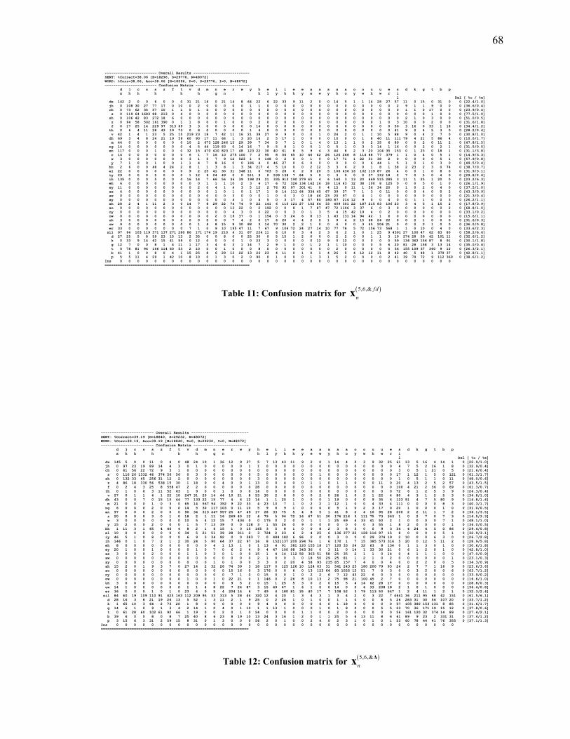
68
------------------------ Overall Results -------------------------- SENT: %Correct=38.06 [H=18296, S=29776, N=48072] WORD: %Corr=38.06, Acc=38.06 [H=18296, D=0, S=29776, I=0, N=48072] ------------------------ Confusion Matrix ------------------------- d j c s s z f t v d m n e r w y h e i i e e a a a a a o o u u e s d k g t b p x h h h h h g n h l y h h y e w y h o y w h w r i l Del [ %c / %e] dx 142 2 0 0 6 0 0 0 31 21 16 0 21 14 8 64 22 6 22 33 9 11 2 0 0 14 5 1 1 14 28 27 57 11 0 15 0 31 0 0 [22.4/1.0] jh 0 108 30 27 77 17 0 10 0 2 0 0 0 0 0 1 1 0 0 0 0 0 0 0 0 0 0 0 0 0 0 0 2 9 1 1 9 0 0 0 [36.6/0.4] ch 0 73 62 35 57 10 1 1 0 1 0 0 0 0 0 0 0 0 0 0 0 0 0 0 0 0 0 0 0 0 0 0 0 1 1 0 17 0 0 0 [23.9/0.4] s 0 119 64 1683 88 213 0 4 0 0 0 0 0 0 0 0 0 0 0 0 0 0 0 0 0 0 0 0 0 0 0 0 0 0 0 0 1 0 0 0 [77.5/1.0] sh 0 106 42 83 272 18 6 0 0 0 0 0 0 0 0 0 0 0 0 0 0 0 0 0 0 0 0 0 0 0 0 0 0 2 1 0 3 0 0 0 [51.0/0.5] z 0 94 58 502 161 390 0 1 1 8 0 0 1 0 0 0 2 0 2 0 0 0 0 0 0 0 0 0 0 0 1 0 3 10 0 0 2 0 0 0 [31.6/1.8] f 0 17 25 14 229 97 313 69 3 3 0 0 0 0 0 0 14 0 0 0 0 0 0 0 0 0 0 0 0 0 0 0 56 3 16 0 33 1 18 0 [34.4/1.2] th 0 6 4 11 28 43 19 73 0 8 0 0 0 0 0 1 4 0 0 0 0 0 0 0 0 0 0 0 0 0 0 0 41 9 0 4 5 3 0 0 [28.2/0.4] v 42 1 4 1 23 5 25 15 219 23 18 7 42 11 16 21 38 27 9 9 0 0 0 1 0 24 2 0 1 1 10 5 88 9 0 4 2 7 0 0 [30.8/1.0] dh 69 3 4 8 24 21 19 59 60 90 17 11 66 1 3 20 16 2 5 17 1 0 0 0 0 10 0 0 1 8 40 11 111 79 4 21 5 86 4 0 [10.0/1.7] m 44 0 0 0 0 0 0 0 10 2 673 128 246 15 29 39 7 34 5 7 1 0 1 4 0 13 1 1 0 2 35 6 89 0 0 2 0 11 2 0 [47.8/1.5] ng 14 0 0 0 0 0 0 0 4 5 44 119 83 0 14 16 7 9 5 8 1 0 0 1 0 5 1 0 3 3 14 1 16 0 0 2 0 2 1 0 [31.5/0.5] en 117 0 0 0 1 0 0 0 32 15 470 410 823 17 48 123 22 30 40 61 8 5 9 4 3 44 8 2 3 20 104 35 153 0 1 23 0 18 1 0 [31.1/3.8] r 14 0 0 0 0 0 0 0 6 1 7 16 10 275 100 7 2 95 8 56 65 10 46 42 26 120 266 8 114 88 77 379 1 1 0 4 0 5 1 0 [14.9/3.3] w 3 0 0 0 0 0 0 0 3 1 5 7 9 12 523 1 0 148 0 2 0 0 1 0 0 17 71 1 22 31 38 2 0 0 0 0 0 5 1 0 [57.9/0.8] y 7 1 0 0 1 0 0 1 1 4 7 8 16 0 0 186 4 0 46 27 0 6 0 0 0 0 0 0 0 6 44 1 5 1 0 1 0 3 0 0 [49.5/0.4] hh 2 6 0 0 48 4 24 2 8 1 1 3 8 1 3 34 217 4 5 10 0 0 2 12 3 3 6 2 0 1 8 1 38 2 23 2 3 0 74 0 [38.7/0.7] el 22 0 0 0 0 0 0 0 9 2 25 41 30 31 348 11 0 703 5 28 6 2 8 20 5 106 436 16 102 119 87 26 4 0 0 1 0 8 0 0 [31.9/3.1] iy 29 0 0 0 5 0 0 0 1 12 9 24 49 0 0 511 9 0 539 138 7 84 5 0 0 3 0 0 0 37 312 18 2 7 0 5 0 4 0 0 [29.8/2.6] ih 135 0 0 0 5 0 0 0 16 14 7 66 56 36 39 198 29 21 335 913 190 279 65 4 6 160 3 13 20 469 515 285 3 11 1 25 1 20 0 0 [23.2/6.3] eh 6 0 0 0 0 0 0 0 0 0 1 1 1 10 2 3 4 17 6 72 326 134 162 16 18 116 43 32 38 100 8 125 0 0 0 5 0 1 0 0 [26.1/1.9] ey 11 0 0 0 0 0 0 0 0 2 0 4 1 4 3 5 12 2 76 95 97 301 41 0 4 15 0 11 1 56 34 20 0 1 0 2 0 4 0 0 [37.5/1.0] ae 4 0 0 0 0 0 0 0 0 0 0 1 0 1 0 1 17 1 8 14 111 64 334 45 67 39 37 7 1 3 0 11 0 0 0 4 0 0 2 0 [43.3/0.9] aw 0 0 0 0 0 0 0 0 0 0 0 0 0 3 0 0 0 1 0 0 3 0 18 46 23 20 97 0 4 1 0 0 0 0 0 0 0 0 0 0 [21.3/0.4] ay 0 0 0 0 0 0 0 0 0 0 0 0 0 4 1 0 4 5 0 3 17 4 57 80 180 87 214 12 9 0 0 4 0 0 1 1 0 0 3 0 [26.2/1.1] ah 28 2 4 1 11 2 3 0 14 7 8 29 22 74 74 9 22 141 6 115 121 27 102 64 33 409 301 22 187 215 83 106 23 3 4 5 1 15 2 0 [17.8/3.9] ao 0 0 0 0 0 0 0 0 0 0 0 0 0 13 22 0 2 192 0 0 8 1 7 87 47 72 1106 3 37 6 0 3 0 0 0 0 0 0 2 0 [68.8/1.0] oy 0 0 0 0 0 0 0 0 0 0 0 0 0 4 3 0 0 22 0 0 3 0 1 3 5 4 15 42 19 4 0 2 0 0 0 0 0 0 0 0 [33.1/0.2] ow 0 0 0 0 0 0 0 0 0 0 0 2 0 19 37 0 1 154 0 5 24 6 8 13 1 43 131 14 94 42 1 6 0 0 0 0 0 0 0 0 [15.6/1.1] uh 3 0 0 0 0 0 0 0 0 0 0 0 0 7 4 2 0 17 6 20 4 4 2 0 1 9 4 2 15 68 24 22 0 0 0 1 0 0 0 0 [31.6/0.3] uw 9 0 0 0 0 0 0 0 0 1 9 8 15 8 30 88 3 14 70 30 2 2 1 0 0 6 0 0 3 45 206 21 0 0 0 0 1 0 0 0 [36.0/0.8] er 33 0 0 0 0 0 0 0 7 1 0 9 10 195 47 11 7 67 9 104 72 24 27 14 10 77 78 5 72 156 73 568 1 1 0 10 0 4 0 0 [33.6/2.3] sil 97 94 103 119 571 137 271 280 86 171 174 19 210 4 31 87 224 11 6 10 0 3 4 2 3 6 2 1 0 1 25 9 4391 27 100 47 62 83 80 0 [58.2/6.6] d 27 25 5 8 59 23 15 13 2 35 0 0 8 0 0 25 30 0 5 15 1 2 0 0 0 2 2 0 0 1 1 3 19 274 28 59 42 101 11 0 [32.6/1.2] k 0 33 9 14 62 15 41 59 0 12 0 0 0 0 1 0 23 3 0 0 0 0 0 12 9 0 12 0 0 0 0 0 59 136 362 156 87 8 91 0 [30.1/1.8] g 12 7 0 0 8 1 4 11 1 17 3 4 4 3 1 14 7 2 9 1 0 0 1 2 1 1 10 0 0 0 5 6 20 81 28 158 3 13 14 0 [35.0/0.6] t 0 78 81 94 146 114 60 53 2 10 0 0 1 0 0 0 8 0 0 0 0 0 0 0 0 2 0 0 0 0 0 0 36 155 109 37 360 9 12 0 [26.3/2.1] b 41 1 0 0 8 0 4 1 15 25 8 6 29 13 22 13 26 23 4 11 0 1 0 1 4 26 5 4 12 12 11 8 42 40 5 48 1 379 37 0 [42.8/1.1] p 5 5 11 4 29 1 42 10 8 10 0 1 3 0 2 0 90 0 1 0 0 0 1 3 1 5 2 0 0 0 0 2 41 39 79 72 9 112 369 0 [38.6/1.2] Ins 0 0 0 0 0 0 0 0 0 0 0 0 0 0 0 0 0 0 0 0 0 0 0 0 0 0 0 0 0 0 0 0 0 0 0 0 0 0 0 ===================================================================
Table 11: Confusion matrix for ( )5,6,& fdnx
------------------------ Overall Results -------------------------- SENT: %Correct=39.19 [H=18840, S=29232, N=48072] WORD: %Corr=39.19, Acc=39.19 [H=18840, D=0, S=29232, I=0, N=48072] ------------------------ Confusion Matrix ------------------------- d j c s s z f t v d m n e r w y h e i i e e a a a a a o o u u e s d k g t b p x h h h h h g n h l y h h y e w y h o y w h w r i l Del [ %c / %e] dx 145 5 0 0 11 0 4 0 48 24 10 1 36 12 9 37 5 7 13 43 11 9 2 0 1 14 4 0 3 9 32 25 61 13 5 16 4 14 1 0 [22.9/1.0] jh 0 97 23 19 89 14 4 3 0 1 0 0 0 0 0 1 1 0 0 0 0 0 0 0 0 0 0 0 0 0 0 0 4 7 5 2 16 1 8 0 [32.9/0.4] ch 0 61 56 22 72 9 3 1 0 0 0 0 0 0 0 0 0 0 0 0 0 0 0 0 0 0 0 0 0 0 0 0 3 0 5 1 21 0 5 0 [21.6/0.4] s 0 116 26 1332 46 374 56 56 0 3 0 0 0 0 0 0 5 0 0 0 0 0 0 1 0 0 0 0 0 0 0 0 17 1 12 1 5 0 121 0 [61.3/1.7] sh 0 132 33 45 256 31 12 2 0 0 0 0 0 0 0 0 3 0 0 0 0 0 0 0 0 0 0 0 0 0 0 0 1 0 5 1 1 0 11 0 [48.0/0.6] z 4 86 18 330 56 538 15 30 1 18 0 0 4 0 0 1 13 0 0 4 0 0 1 1 0 1 1 0 0 0 11 0 20 4 13 2 5 2 57 0 [43.5/1.5] f 0 2 4 3 25 8 558 47 2 2 0 0 0 0 0 0 28 0 0 0 0 0 0 0 0 0 0 0 0 0 0 0 100 4 21 2 36 0 69 0 [61.3/0.7] th 0 1 0 6 3 11 52 63 1 9 0 0 1 0 0 0 14 0 0 0 0 0 0 0 0 0 0 0 0 0 0 0 72 6 1 2 5 3 9 0 [24.3/0.4] v 27 0 1 1 4 1 22 10 247 31 20 14 44 10 21 8 53 30 2 8 0 0 0 2 0 26 1 0 2 1 22 4 80 4 3 1 2 5 3 0 [34.8/1.0] dh 43 0 0 7 0 15 15 44 77 133 22 15 77 4 6 12 14 1 1 20 1 0 0 0 1 19 0 0 0 9 35 6 123 91 4 7 5 80 9 0 [14.8/1.6] m 21 0 0 0 1 0 3 0 65 14 567 94 352 9 22 33 4 23 10 7 1 0 2 2 1 12 1 0 0 4 33 4 111 0 0 0 0 8 3 0 [40.3/1.7] ng 6 0 0 0 2 0 0 0 14 5 30 117 103 0 11 10 5 9 6 9 1 0 0 0 0 5 1 0 2 3 17 0 20 1 0 0 0 1 0 0 [31.0/0.5] en 97 0 0 0 2 0 0 0 90 34 313 447 957 25 47 49 17 28 33 75 5 4 8 5 1 41 8 2 4 10 95 28 200 2 2 11 1 7 2 0 [36.1/3.5] r 20 0 0 0 3 0 1 0 18 2 1 11 16 269 40 12 4 79 5 96 72 16 67 51 30 176 214 5 111 75 73 363 1 0 2 7 0 7 3 0 [14.5/3.3] w 3 0 0 0 0 0 0 0 10 5 4 12 15 7 434 0 0 175 0 2 0 0 1 1 1 25 69 4 33 41 50 2 1 0 0 0 0 7 1 0 [48.1/1.0] y 15 2 0 0 2 0 0 0 1 5 7 13 39 0 0 128 3 1 55 26 0 9 0 0 0 0 0 0 0 3 55 1 8 2 0 0 0 0 1 0 [34.0/0.5] hh 1 11 3 1 65 4 46 4 8 2 1 6 15 1 3 15 165 3 5 8 1 0 0 8 2 3 8 3 0 0 9 3 34 4 24 4 5 0 86 0 [29.4/0.8] el 10 0 0 0 0 0 0 0 34 5 21 51 39 28 311 2 3 724 2 23 6 2 4 25 6 136 377 22 128 116 97 15 8 0 0 0 0 5 1 0 [32.9/3.1] iy 46 5 1 0 8 0 0 0 6 9 3 34 92 0 0 383 7 0 484 182 6 96 2 0 0 3 0 0 0 29 374 19 2 10 0 0 6 3 0 0 [26.7/2.8] ih 146 0 1 0 7 2 1 2 30 24 5 90 64 37 22 97 16 8 1521137 200 294 76 1 6 170 1 7 15 385 573 316 5 20 0 12 5 11 2 0 [28.9/5.8] eh 8 0 0 0 0 0 0 0 0 0 0 4 1 13 1 0 1 13 4 91 381 120 155 18 17 120 33 24 32 63 8 134 0 1 1 3 0 1 0 0 [30.6/1.8] ey 20 1 0 0 1 0 0 0 0 1 0 7 0 6 2 4 9 4 47 100 98 343 36 0 3 11 0 14 1 33 30 21 0 6 1 2 0 1 0 0 [42.8/1.0] ae 3 0 0 0 2 0 0 0 1 1 0 3 0 1 0 0 15 1 4 14 112 58 363 51 58 25 35 2 1 1 0 14 0 4 1 1 1 0 0 0 [47.0/0.9] aw 0 0 0 0 0 0 0 0 0 0 0 0 0 0 0 0 2 1 0 0 3 0 18 50 29 25 81 1 2 1 0 2 0 0 0 0 0 0 1 0 [23.1/0.3] ay 0 0 0 0 0 0 0 0 0 0 0 1 0 1 0 0 3 3 0 2 20 4 58 93 235 85 157 7 4 0 0 4 0 0 2 2 0 0 5 0 [34.3/0.9] ah 15 2 0 1 9 3 7 0 27 14 2 32 26 74 39 3 18 117 0 125 126 10 124 63 31 541 243 25 180 200 79 93 24 2 7 7 1 16 9 0 [23.6/3.6] ao 0 0 0 0 0 0 0 0 0 0 0 0 0 15 16 0 3 176 0 0 6 0 13 123 64 83 1025 12 51 7 0 3 0 0 3 2 0 0 6 0 [63.7/1.2] oy 0 0 0 0 0 0 0 0 0 0 0 0 0 7 1 0 0 15 0 0 1 0 2 2 6 7 12 43 22 6 0 3 0 0 0 0 0 0 0 0 [33.9/0.2] ow 0 0 0 0 0 0 0 0 1 0 0 1 0 22 21 0 1 146 0 2 26 8 10 13 2 75 98 21 100 45 2 7 0 0 0 0 0 0 0 0 [16.6/1.0] uh 3 0 0 0 0 0 0 0 0 0 0 0 0 9 5 2 0 15 1 25 5 3 0 2 0 15 5 4 14 62 28 17 0 0 0 0 0 0 0 0 [28.8/0.3] uw 14 1 0 0 0 0 0 0 1 1 4 8 22 7 24 87 3 15 49 47 1 6 1 0 0 14 0 0 4 33 208 18 2 1 0 1 0 0 0 0 [36.4/0.8] er 36 0 0 0 1 0 1 0 23 4 0 5 4 204 14 6 7 49 4 180 81 35 40 17 7 108 52 3 79 113 50 547 1 2 4 11 1 2 1 0 [32.3/2.4] sil 84 60 19 109 110 91 423 163 112 209 95 33 313 5 28 44 320 12 4 20 1 3 4 3 1 3 4 2 0 3 22 7 4641 36 211 95 68 42 151 0 [61.5/6.1] d 28 16 3 8 21 19 26 13 5 52 1 3 11 2 1 9 25 0 2 26 1 0 1 0 0 1 1 0 0 0 8 5 26 283 31 30 56 107 20 0 [33.7/1.2] k 1 65 10 3 64 2 73 20 1 8 0 0 0 0 0 0 9 4 0 0 0 0 0 6 0 1 18 0 0 0 0 0 57 105 380 153 131 8 85 0 [31.6/1.7] g 14 6 1 0 9 1 3 4 2 14 1 0 4 0 1 10 1 1 13 1 0 0 0 1 0 1 8 0 0 0 5 5 23 70 36 171 19 15 12 0 [37.8/0.6] t 0 61 28 60 102 61 92 66 1 19 0 0 2 0 1 0 24 0 0 0 0 1 1 0 0 2 0 0 0 0 0 0 56 161 120 32 374 14 89 0 [27.4/2.1] b 39 6 0 0 8 0 8 7 25 40 8 6 23 8 19 10 13 24 3 16 1 2 0 1 1 25 5 4 13 11 8 6 61 89 9 23 2 331 31 0 [37.4/1.2] p 3 15 6 3 31 2 59 15 8 31 0 1 3 0 0 0 56 2 0 1 0 0 2 4 0 2 3 1 0 1 0 1 53 60 78 44 41 76 355 0 [37.1/1.3] Ins 0 0 0 0 0 0 0 0 0 0 0 0 0 0 0 0 0 0 0 0 0 0 0 0 0 0 0 0 0 0 0 0 0 0 0 0 0 0 0 ===================================================================
Table 12: Confusion matrix for ( )5,6,&n
∆x

69
------------------------ Overall Results -------------------------- SENT: %Correct=50.34 [H=24199, S=23873, N=48072] WORD: %Corr=50.34, Acc=50.34 [H=24199, D=0, S=23873, I=0, N=48072] ------------------------ Confusion Matrix ------------------------- d j c s s z f t v d m n e r w y h e i i e e a a a a a o o u u e s d k g t b p x h h h h h g n h l y h h y e w y h o y w h w r i l Del [ %c / %e] dx 291 4 0 0 7 3 0 1 11 16 6 3 17 16 1 18 2 4 5 36 1 3 0 0 0 32 0 0 2 2 6 1 31 24 2 27 2 58 2 0 [45.9/0.7] jh 1 83 79 10 97 6 1 0 0 0 0 0 0 0 0 0 2 0 0 0 0 0 0 0 0 0 0 0 0 0 0 1 0 2 1 1 9 2 0 0 [28.1/0.4] ch 0 34 110 9 88 1 1 0 0 0 0 0 0 0 0 0 0 0 0 0 0 0 0 0 0 0 0 0 0 0 0 0 0 0 0 0 16 0 0 0 [42.5/0.3] s 0 70 68 1536 63 313 7 64 0 0 0 0 0 0 0 0 0 0 0 0 0 0 0 0 0 0 0 0 0 0 0 0 0 0 3 0 48 0 0 0 [70.7/1.3] sh 0 90 101 20 298 7 4 1 0 0 0 0 0 0 0 1 0 0 0 0 0 0 0 0 0 0 0 0 0 0 0 0 0 0 0 0 11 0 0 0 [55.9/0.5] z 2 58 21 297 59 718 3 29 1 11 0 0 1 0 0 0 1 0 0 1 0 0 0 0 0 0 0 0 0 0 0 0 1 5 0 3 25 0 0 0 [58.1/1.1] f 0 1 1 3 4 0 695 110 8 5 0 0 0 0 0 0 2 0 0 0 0 0 0 0 0 0 0 0 0 0 0 0 32 2 3 0 22 3 20 0 [76.3/0.4] th 0 0 1 9 0 3 18 161 1 10 0 1 1 0 0 0 1 0 0 0 0 0 0 0 0 0 0 0 0 0 0 0 34 2 0 0 12 1 4 0 [62.2/0.2] v 32 0 0 0 0 0 40 12 397 36 9 1 13 7 14 0 2 5 1 10 0 0 0 0 0 18 0 0 0 1 7 2 53 8 1 9 2 27 3 0 [55.9/0.7] dh 26 0 0 15 0 11 13 66 56 300 16 6 34 0 1 2 1 5 0 24 1 0 0 0 0 26 0 0 0 3 1 0 71 68 0 17 19 97 17 0 [33.5/1.2] m 37 0 0 0 0 0 0 0 44 19 711 123 266 13 14 1 3 10 0 18 0 0 3 3 0 16 1 0 3 4 39 7 49 1 0 10 0 12 0 0 [50.5/1.4] ng 4 0 0 0 0 0 0 0 5 1 47 183 84 0 8 2 1 3 2 9 0 1 2 0 0 7 1 0 1 0 2 0 9 2 0 2 0 2 0 0 [48.4/0.4] en 189 0 0 0 0 1 0 0 34 46 271 3611206 7 36 23 16 30 15 100 14 5 5 3 0 81 4 2 5 6 34 4 95 15 0 24 0 18 0 0 [45.5/3.0] r 45 0 0 0 1 0 0 0 32 2 7 3 0 874 22 11 1 8 8 49 23 6 14 13 11 49 81 23 13 8 9 518 0 1 0 4 0 14 0 0 [47.2/2.0] w 3 0 0 0 0 0 0 0 14 1 6 16 9 19 514 0 0 118 0 1 0 0 0 1 0 35 45 43 28 15 19 0 0 0 0 1 0 13 2 0 [56.9/0.8] y 8 0 0 0 1 0 0 0 0 0 2 8 3 1 0 170 6 0 95 28 0 22 0 0 0 1 0 0 0 0 12 2 2 2 2 5 1 5 0 0 [45.2/0.4] hh 5 4 0 0 3 1 2 1 4 2 2 3 8 1 1 13 309 3 10 10 1 5 2 3 0 7 0 0 1 0 0 3 21 17 37 13 24 1 44 0 [55.1/0.5] el 7 0 0 0 0 0 0 0 20 27 26 24 13 11 152 0 1 1136 2 30 5 1 4 23 3 175 206 95 128 61 26 1 3 2 1 1 0 16 1 0 [51.6/2.2] iy 8 0 0 0 0 0 0 0 1 0 1 29 13 3 0 367 11 1 852 166 7 176 8 0 0 2 0 3 0 11 124 25 1 0 0 1 0 0 0 0 [47.1/2.0] ih 202 0 0 0 1 2 0 0 27 53 11 54 84 60 3 107 21 14 1941325 260 401 113 8 14 329 0 28 29 197 192 129 7 27 0 24 2 20 2 0 [33.6/5.4] eh 5 0 0 0 0 0 0 0 1 0 1 6 5 35 0 0 4 7 6 111 313 136 196 19 39 176 19 35 20 20 3 90 0 0 0 0 0 0 0 0 [25.1/1.9] ey 0 0 0 0 0 0 0 0 0 0 0 11 3 5 0 2 4 0 59 106 69 417 71 3 2 1 0 11 1 14 13 9 1 0 0 0 0 0 0 0 [52.0/0.8] ae 0 0 0 0 0 0 0 0 0 0 0 1 0 10 0 0 12 0 1 29 107 57 392 37 81 27 9 3 0 1 0 4 0 0 0 0 0 0 1 0 [50.8/0.8] aw 0 0 0 0 0 0 0 0 0 0 0 0 0 4 0 0 1 3 0 0 6 0 18 52 44 25 56 3 1 2 0 1 0 0 0 0 0 0 0 0 [24.1/0.3] ay 0 0 0 0 0 0 0 0 0 0 0 0 0 14 0 0 1 2 0 2 29 7 85 134 241 76 80 9 1 2 0 3 0 0 0 0 0 0 0 0 [35.1/0.9] ah 49 2 0 0 1 5 0 0 28 30 7 8 33 74 24 3 9 155 0 148 105 7 59 83 57 796 173 57 125 126 18 22 11 19 5 11 3 33 9 0 [34.7/3.1] ao 0 0 0 0 0 0 0 0 0 0 0 1 0 98 88 0 1 81 0 1 5 0 15 149 99 85 831 97 45 2 2 8 0 0 0 0 0 0 0 0 [51.7/1.6] oy 0 0 0 0 0 0 0 0 0 0 0 0 0 1 2 0 0 5 0 0 3 1 0 12 1 5 9 63 19 2 0 4 0 0 0 0 0 0 0 0 [49.6/0.1] ow 4 0 0 0 0 0 0 0 0 0 0 0 1 10 28 0 0 102 0 10 10 0 2 18 9 80 52 92 133 40 7 3 0 0 0 0 0 0 0 0 [22.1/1.0] uh 4 0 0 0 0 0 0 0 2 0 1 1 2 3 2 0 0 19 0 38 6 4 0 0 2 41 3 10 19 34 15 8 0 0 0 1 0 0 0 0 [15.8/0.4] uw 11 0 0 0 0 0 0 0 4 0 10 4 6 9 21 49 2 15 53 67 2 15 3 0 0 18 0 3 8 41 204 23 1 0 0 2 0 1 0 0 [35.7/0.8] er 24 0 0 0 0 0 0 0 11 1 1 1 6 484 11 5 4 3 5 77 37 13 17 4 9 27 30 13 9 25 15 855 3 0 1 0 0 1 0 0 [50.5/1.7] sil 232 76 22 34 73 78 54 161 199 318 98 56 184 14 25 29 69 15 10 21 2 1 0 0 1 9 0 0 0 2 10 12 5196 128 67 115 72 77 91 0 [68.8/4.9] d 98 11 5 5 18 9 11 6 11 36 0 1 1 0 0 6 14 0 0 14 2 1 0 0 0 5 0 0 0 2 0 0 23 325 13 47 69 86 22 0 [38.6/1.1] k 1 10 7 4 9 8 6 3 1 10 0 0 0 0 0 1 49 1 0 1 0 0 2 0 0 0 1 0 0 0 0 0 34 40 682 195 43 8 88 0 [56.6/1.1] g 16 6 0 0 1 2 0 1 3 9 1 0 1 2 1 7 7 1 5 5 1 0 0 0 0 2 2 0 0 0 0 5 12 11 75 234 7 29 6 0 [51.8/0.5] t 10 52 60 60 54 32 25 45 2 20 0 0 1 0 0 1 17 1 0 1 1 0 0 0 0 2 0 0 0 0 1 0 40 216 23 13 620 14 56 0 [45.4/1.6] b 55 3 2 0 0 0 3 0 43 36 1 1 2 5 7 6 8 13 1 7 1 1 0 1 0 20 1 0 2 3 0 0 33 57 3 23 9 505 34 0 [57.0/0.8] p 7 4 5 2 3 3 18 11 7 22 0 1 1 2 0 0 65 1 0 2 0 0 0 0 0 5 0 0 0 0 0 2 46 50 37 19 51 156 437 0 [45.7/1.1] Ins 0 0 0 0 0 0 0 0 0 0 0 0 0 0 0 0 0 0 0 0 0 0 0 0 0 0 0 0 0 0 0 0 0 0 0 0 0 0 0 ===================================================================
Table 13: Confusion matrix for c t
------------------------ Overall Results -------------------------- SENT: %Correct=54.86 [H=26372, S=21700, N=48072] WORD: %Corr=54.86, Acc=54.86 [H=26372, D=0, S=21700, I=0, N=48072] ------------------------ Confusion Matrix ------------------------- d j c s s z f t v d m n e r w y h e i i e e a a a a a o o u u e s d k g t b p x h h h h h g n h l y h h y e w y h o y w h w r i l Del [ %c / %e] dx 383 1 0 0 2 2 0 1 2 9 1 1 6 8 3 15 1 0 0 16 0 0 0 0 0 13 0 0 0 1 1 0 14 41 0 19 0 91 3 0 [60.4/0.5] jh 4 112 66 7 40 7 1 1 0 0 0 0 0 0 0 0 1 0 0 1 0 0 0 0 0 0 0 0 0 0 0 0 5 31 2 3 14 0 0 0 [38.0/0.4] ch 0 49 157 11 28 2 1 0 0 0 0 0 0 0 0 0 0 0 0 0 0 0 0 0 0 0 0 0 0 0 0 0 0 2 0 0 9 0 0 0 [60.6/0.2] s 0 37 37 1621 96 285 22 28 0 0 0 0 0 0 0 0 0 0 0 0 0 0 0 0 0 0 0 0 0 0 0 0 4 13 0 0 28 0 1 0 [74.6/1.1] sh 0 25 51 28 406 12 6 0 0 0 0 0 0 0 0 0 0 0 0 0 0 0 0 0 0 0 0 0 0 0 0 0 1 0 0 0 3 0 1 0 [76.2/0.3] z 2 50 12 272 65 744 5 16 6 7 0 0 0 0 0 0 3 0 0 0 0 0 0 0 0 0 0 0 0 0 0 0 21 19 1 2 9 0 2 0 [60.2/1.0] f 2 2 1 2 2 2 698 116 11 5 0 0 0 0 0 0 1 0 0 0 0 0 0 0 0 0 0 0 0 0 0 0 19 14 2 2 12 3 17 0 [76.6/0.4] th 3 1 0 8 0 2 41 153 1 5 0 0 0 0 0 0 1 0 0 0 0 0 0 0 0 0 0 0 0 0 0 0 24 9 0 0 6 4 1 0 [59.1/0.2] v 48 0 0 0 2 3 28 6 370 43 11 7 10 4 7 0 9 4 1 10 0 0 0 0 0 28 0 0 1 3 2 1 54 15 0 1 0 42 0 0 [52.1/0.7] dh 110 0 0 6 0 4 10 38 55 156 7 4 23 0 4 1 4 0 0 9 0 0 0 0 0 20 0 0 0 0 0 0 51 120 1 29 11 228 5 0 [17.4/1.5] m 81 0 0 0 0 0 0 0 35 9 706 97 285 8 13 2 2 7 1 18 1 1 5 0 0 34 1 0 5 6 19 4 27 1 0 5 0 34 0 0 [50.2/1.5] ng 17 0 0 0 0 0 0 0 2 2 18 191 93 1 1 4 0 7 1 10 2 0 1 0 0 7 2 0 1 1 5 1 8 0 0 1 0 2 0 0 [50.5/0.4] en 336 1 0 0 0 0 0 0 19 32 210 3441150 7 16 17 5 21 5 100 4 5 6 1 2 98 1 0 3 7 22 6 79 10 0 47 0 95 1 0 [43.4/3.1] r 100 0 0 0 0 0 0 0 15 1 9 1 4 1056 27 10 0 21 5 59 15 10 12 5 18 81 44 10 8 7 7 281 2 0 1 19 0 22 0 0 [57.1/1.7] w 24 0 0 0 0 0 0 0 12 2 8 3 13 16 619 0 0 65 0 1 1 0 0 1 1 43 13 20 3 9 13 0 3 1 0 3 0 29 0 0 [68.5/0.6] y 33 0 0 0 0 0 0 0 1 0 1 2 6 0 0 225 3 0 38 38 3 2 2 0 0 0 0 0 0 0 3 0 3 5 1 7 0 3 0 0 [59.8/0.3] hh 18 4 0 1 5 2 4 3 9 3 3 2 6 1 3 10 302 7 9 11 1 1 0 2 2 6 3 0 0 0 0 0 19 31 16 20 8 8 41 0 [53.8/0.5] el 41 0 0 0 0 0 0 0 7 11 26 22 23 21 219 1 1 1150 4 23 2 2 0 29 17 256 96 14 132 40 14 0 5 3 2 5 0 35 0 0 [52.2/2.2] iy 16 0 0 0 0 0 0 0 1 0 4 25 20 2 0 158 0 1 1156 154 4 172 1 0 3 1 0 20 1 2 58 6 5 0 0 0 0 0 0 0 [63.9/1.4] ih 367 1 0 0 0 2 0 0 11 21 17 38 102 63 4 137 10 18 1811636 213 245 49 4 29 318 2 24 46 95 127 66 14 17 0 41 0 42 0 0 [41.5/4.8] eh 5 0 0 0 0 0 0 0 0 0 0 5 3 31 2 9 5 4 3 169 388 71 196 48 31 119 24 9 33 19 9 63 0 0 0 0 0 0 1 0 [31.1/1.8] ey 0 0 0 0 0 0 0 0 0 0 0 1 4 1 0 5 0 0 74 48 22 546 26 0 31 0 0 29 0 4 6 4 1 0 0 0 0 0 0 0 [68.1/0.5] ae 0 0 0 0 0 0 0 0 0 0 0 2 1 0 0 0 1 1 6 39 122 19 428 56 45 28 9 0 4 0 4 6 1 0 0 0 0 0 0 0 [55.4/0.7] aw 0 0 0 0 0 0 0 0 0 0 0 0 0 0 0 0 0 3 0 0 3 0 27 123 5 14 32 0 7 0 0 2 0 0 0 0 0 0 0 0 [56.9/0.2] ay 0 0 0 0 0 0 0 0 0 0 0 0 0 3 0 0 0 1 0 1 3 11 32 19 491 28 74 18 1 0 0 4 0 0 0 0 0 0 0 0 [71.6/0.4] ah 140 0 0 0 1 2 0 1 11 15 9 7 20 57 39 0 7 109 1 150 91 10 68 55 83 907 133 35 92 71 14 22 15 29 1 35 2 62 1 0 [39.5/2.9] ao 1 0 0 0 0 0 0 0 0 0 0 0 0 28 36 0 3 65 0 1 3 1 22 99 92 66 1078 33 40 4 1 32 0 0 1 2 0 0 0 0 [67.0/1.1] oy 0 0 0 0 0 0 0 0 0 0 0 0 0 0 1 0 0 0 0 0 0 3 0 0 5 0 5 110 0 0 0 3 0 0 0 0 0 0 0 0 [86.6/0.0] ow 0 0 0 0 0 0 0 0 0 0 0 0 1 5 4 0 0 111 0 4 18 2 8 49 5 48 38 8 276 8 8 7 1 0 0 0 0 0 0 0 [45.9/0.7] uh 1 0 0 0 0 0 0 0 0 0 1 0 2 5 2 0 0 15 1 38 15 6 0 0 0 48 12 8 9 38 8 6 0 0 0 0 0 0 0 0 [17.7/0.4] uw 20 0 0 0 0 0 0 0 1 0 11 4 16 9 10 41 0 16 36 79 4 6 4 0 0 11 1 7 18 10 250 16 1 0 0 0 0 1 0 0 [43.7/0.7] er 22 0 0 0 0 0 0 0 2 0 2 4 3 289 2 4 2 8 7 102 54 18 15 4 10 55 27 16 9 6 18 1002 7 0 0 3 0 1 0 0 [59.2/1.4] sil 560 38 1 6 6 17 67 136 125 97 87 63 168 11 17 16 56 13 8 21 1 0 0 0 3 26 0 0 1 1 3 7 4884 430 37 170 117 234 124 0 [64.7/5.5] d 89 12 2 0 2 1 2 3 1 13 0 0 4 0 0 2 2 0 0 1 1 0 0 0 0 2 0 0 0 0 0 0 16 390 7 47 32 203 9 0 [46.4/0.9] k 5 7 4 3 4 2 4 2 0 2 0 0 0 0 1 0 25 2 1 2 0 1 0 0 0 1 0 1 0 0 0 0 20 123 597 296 45 25 31 0 [49.6/1.3] g 20 2 0 0 1 0 0 0 0 1 0 0 2 5 2 10 2 1 0 1 0 0 0 1 0 1 0 0 0 0 0 0 7 70 30 217 4 74 1 0 [48.0/0.5] t 8 41 39 22 9 11 21 12 0 11 0 0 1 0 0 1 4 1 0 0 0 0 0 0 0 2 0 0 0 0 0 0 32 402 44 31 608 39 28 0 [44.5/1.6] b 92 1 0 0 0 0 1 0 0 5 0 0 1 1 21 1 0 0 0 0 0 0 0 0 0 3 0 0 0 0 0 0 9 74 0 32 0 631 14 0 [71.2/0.5] p 15 3 0 0 5 1 15 11 1 9 0 0 0 2 0 0 27 0 0 0 0 0 0 0 0 4 0 0 0 0 0 0 34 101 25 47 15 225 417 0 [43.6/1.1] Ins 0 0 0 0 0 0 0 0 0 0 0 0 0 0 0 0 0 0 0 0 0 0 0 0 0 0 0 0 0 0 0 0 0 0 0 0 0 0 0 ===================================================================
Table 14: Confusion matrix for O t

70
------------------------ Overall Results -------------------------- SENT: %Correct=55.04 [H=26460, S=21612, N=48072] WORD: %Corr=55.04, Acc=55.04 [H=26460, D=0, S=21612, I=0, N=48072] ------------------------ Confusion Matrix ------------------------- d j c s s z f t v d m n e r w y h e i i e e a a a a a o o u u e s d k g t b p x h h h h h g n h l y h h y e w y h o y w h w r i l Del [ %c / %e] dx 216 0 0 0 1 0 0 0 2 14 4 1 13 8 3 9 7 2 1 12 0 0 0 0 0 11 0 0 0 2 0 0 30 119 1 162 3 12 1 0 [34.1/0.9] jh 2 118 54 10 53 3 1 1 0 1 0 0 0 0 0 0 2 0 0 0 0 0 0 0 0 0 0 0 0 0 0 1 2 23 0 3 21 0 0 0 [40.0/0.4] ch 0 29 152 14 39 2 0 0 0 0 0 0 0 0 0 0 0 0 0 0 0 0 0 0 0 0 0 0 0 0 0 0 0 3 0 0 20 0 0 0 [58.7/0.2] s 0 21 40 1634 90 309 16 26 1 0 0 0 0 0 0 0 0 0 0 0 0 0 0 0 0 0 0 0 0 0 0 0 3 8 0 0 24 0 0 0 [75.2/1.1] sh 0 27 57 36 394 10 3 0 0 0 0 0 0 0 0 0 0 0 0 0 0 0 0 0 0 0 0 0 0 0 0 0 1 0 0 0 5 0 0 0 [73.9/0.3] z 2 27 21 297 51 742 9 10 3 20 1 0 0 0 0 0 4 0 1 1 0 0 0 0 0 0 0 0 0 0 0 0 16 8 0 0 23 0 0 0 [60.0/1.0] f 1 0 1 3 3 0 709 84 7 20 0 0 0 0 0 0 4 0 0 0 0 0 0 0 0 0 0 0 0 0 0 0 34 6 2 1 27 1 8 0 [77.8/0.4] th 1 1 1 10 0 4 41 130 2 24 0 0 0 0 0 0 1 0 0 0 0 0 0 0 0 0 0 0 0 0 0 0 26 3 0 5 10 0 0 0 [50.2/0.3] v 17 0 0 0 1 4 32 6 317 95 31 0 15 2 10 0 17 5 3 7 1 0 0 0 0 10 0 0 1 3 3 3 66 24 0 27 3 7 0 0 [44.6/0.8] dh 49 0 0 0 0 5 8 33 15 235 22 2 21 1 1 2 12 2 0 2 1 0 0 0 0 15 0 0 0 0 0 0 105 230 0 101 12 22 0 0 [26.2/1.4] m 24 0 0 0 0 0 0 0 17 14 793 56 290 11 6 1 5 7 1 16 0 0 2 0 0 19 0 1 0 4 13 4 46 20 0 48 0 8 1 0 [56.4/1.3] ng 0 0 0 0 0 0 0 0 1 1 42 136 126 1 1 1 4 6 5 9 0 0 0 0 0 5 1 0 4 0 8 1 7 4 0 15 0 0 0 0 [36.0/0.5] en 127 0 0 0 0 0 0 0 11 23 279 1711319 4 7 12 16 21 6 88 6 3 3 1 1 69 3 1 7 8 21 4 110 79 3 228 1 18 0 0 [49.8/2.8] r 50 0 0 0 0 0 0 0 14 8 13 2 4 925 20 10 2 18 10 34 14 12 16 14 19 66 65 12 8 6 11 373 2 18 0 101 0 3 0 0 [50.0/1.9] w 8 0 0 0 0 0 0 0 7 7 18 1 10 19 627 0 3 63 0 0 1 0 0 0 2 9 26 28 4 6 15 1 1 4 0 36 0 7 0 0 [69.4/0.6] y 18 1 0 0 0 0 0 0 0 2 0 2 7 0 0 220 6 0 41 18 1 2 1 0 0 1 0 1 0 0 8 2 3 7 0 34 1 0 0 0 [58.5/0.3] hh 6 2 0 0 0 2 2 1 5 13 7 1 3 2 2 11 370 2 6 7 0 1 0 2 1 3 4 0 1 0 0 0 30 22 6 17 11 1 20 0 [66.0/0.4] el 17 0 0 0 0 0 0 0 7 11 61 15 27 23 214 3 5 1196 11 19 1 6 2 26 19 130 118 21 132 31 16 5 10 15 0 55 0 5 0 0 [54.3/2.1] iy 1 0 0 0 0 0 0 0 0 0 4 12 33 1 0 165 4 2 1149 148 7 182 3 0 1 0 0 18 1 5 54 9 5 1 0 5 0 0 0 0 [63.5/1.4] ih 114 0 0 0 0 1 0 0 9 20 28 29 135 43 5 103 22 7 1691665 241 240 56 8 37 266 5 36 51 117 125 96 14 79 1 210 0 8 0 0 [42.3/4.7] eh 3 0 0 0 0 0 0 0 0 1 0 5 5 20 2 8 8 4 6 166 428 54 148 51 28 123 22 6 42 19 5 92 0 1 0 0 0 0 0 0 [34.3/1.7] ey 0 0 0 0 0 0 0 0 0 0 0 5 5 1 0 4 0 0 73 57 24 546 18 0 30 0 0 28 0 2 4 4 1 0 0 0 0 0 0 0 [68.1/0.5] ae 0 0 0 0 0 0 0 0 0 0 0 1 5 2 0 0 3 1 9 32 131 13 416 59 42 26 18 0 5 0 2 6 1 0 0 0 0 0 0 0 [53.9/0.7] aw 0 0 0 0 0 0 0 0 0 0 0 0 0 0 0 0 0 4 0 0 3 0 25 131 2 12 32 0 7 0 0 0 0 0 0 0 0 0 0 0 [60.6/0.2] ay 0 0 0 0 0 0 0 0 0 0 0 0 0 3 0 0 1 1 0 0 7 16 16 11 478 53 73 18 3 2 0 4 0 0 0 0 0 0 0 0 [69.7/0.4] ah 29 1 0 0 0 3 0 0 15 11 14 4 36 45 14 0 13 117 1 183 89 7 82 63 66 869 138 34 117 78 14 24 28 51 1 132 2 14 0 0 [37.9/3.0] ao 0 0 0 0 0 0 0 0 0 0 0 0 0 35 36 0 2 88 0 2 2 0 22 115 90 64 1036 33 44 6 3 27 0 0 0 3 0 0 0 0 [64.4/1.2] oy 0 0 0 0 0 0 0 0 0 0 0 0 0 2 2 0 0 0 0 1 0 1 0 0 3 4 5 109 0 0 0 0 0 0 0 0 0 0 0 0 [85.8/0.0] ow 0 0 0 0 0 0 0 0 0 0 0 0 1 2 1 0 0 121 0 5 11 2 11 39 4 59 45 6 269 12 5 7 1 0 0 0 0 0 0 0 [44.8/0.7] uh 1 0 0 0 0 0 0 0 0 0 4 0 2 2 0 0 0 19 0 42 9 2 0 0 1 43 8 9 9 49 7 7 0 0 0 1 0 0 0 0 [22.8/0.3] uw 5 0 0 0 0 0 0 0 1 0 15 1 18 10 10 25 1 19 44 70 9 6 2 1 0 13 2 6 20 9 260 18 2 0 0 5 0 0 0 0 [45.5/0.6] er 11 0 0 0 0 0 0 0 7 2 4 2 10 259 3 1 4 8 7 99 53 10 20 7 14 38 24 15 8 6 10 1052 5 3 0 10 0 0 0 0 [62.2/1.3] sil 107 10 7 8 10 24 59 83 79 149 129 42 209 7 15 8 126 17 4 22 1 0 0 0 2 17 0 0 1 0 7 5 5279 666 24 342 42 14 36 0 [69.9/4.7] d 12 8 1 2 1 2 2 0 1 14 0 0 1 1 0 2 10 0 0 3 0 0 0 0 0 0 0 0 0 0 2 0 39 539 8 147 40 5 1 0 [64.1/0.6] k 2 6 4 3 2 1 7 3 1 19 0 0 0 0 0 0 80 0 0 1 0 0 0 0 0 3 0 1 0 0 0 0 34 140 539 242 91 3 22 0 [44.8/1.4] g 5 1 0 0 0 0 0 0 0 6 2 0 0 2 0 5 18 2 0 2 0 0 0 0 0 3 0 0 0 0 0 0 15 81 35 265 4 4 2 0 [58.6/0.4] t 2 25 25 22 8 13 13 18 1 20 0 0 1 0 0 0 11 1 0 0 0 0 0 0 0 1 0 0 0 0 0 0 55 388 19 60 663 4 17 0 [48.5/1.5] b 22 0 0 0 0 0 1 0 2 12 0 0 0 1 11 0 6 5 0 0 0 0 0 0 0 6 0 0 0 0 0 0 77 396 0 182 2 158 5 0 [17.8/1.5] p 6 2 0 0 3 1 21 7 3 33 0 0 0 0 0 0 101 0 0 0 0 0 0 0 0 1 0 0 0 0 0 1 91 187 16 86 38 33 327 0 [34.2/1.3] Ins 0 0 0 0 0 0 0 0 0 0 0 0 0 0 0 0 0 0 0 0 0 0 0 0 0 0 0 0 0 0 0 0 0 0 0 0 0 0 0 ===================================================================
Table 15: Confusion matrix for , 0n ρ =y
------------------------ Overall Results -------------------------- SENT: %Correct=57.85 [H=27810, S=20262, N=48072] WORD: %Corr=57.85, Acc=57.85 [H=27810, D=0, S=20262, I=0, N=48072] ------------------------ Confusion Matrix ------------------------- d j c s s z f t v d m n e r w y h e i i e e a a a a a o o u u e s d k g t b p x h h h h h g n h l y h h y e w y h o y w h w r i l Del [ %c / %e] dx 280 0 0 0 1 0 0 0 3 14 4 2 14 15 7 26 2 3 0 27 0 0 0 0 0 27 0 0 0 0 2 1 41 70 0 79 2 14 0 0 [44.2/0.7] jh 1 129 53 11 51 6 1 1 0 0 0 0 0 0 0 0 1 0 0 0 0 0 0 0 0 0 0 0 0 0 0 1 2 17 1 0 20 0 0 0 [43.7/0.3] ch 0 32 145 18 38 4 0 0 0 0 0 0 0 0 0 0 0 0 0 0 0 0 0 0 0 0 0 0 0 0 0 0 0 1 0 0 21 0 0 0 [56.0/0.2] s 0 32 42 1639 100 295 21 14 0 0 0 0 0 0 0 0 0 0 0 0 0 0 0 0 0 0 0 0 0 0 0 0 1 6 1 0 21 0 0 0 [75.5/1.1] sh 0 31 44 50 391 10 3 0 0 0 0 0 0 0 0 0 1 0 0 0 0 0 0 0 0 0 0 0 0 0 0 0 0 0 0 0 3 0 0 0 [73.4/0.3] z 1 35 26 292 60 748 8 11 3 19 0 0 0 0 0 1 2 0 1 1 0 0 0 0 0 0 0 0 0 0 0 0 10 5 0 0 13 0 0 0 [60.5/1.0] f 1 0 1 3 3 0 709 80 5 9 0 0 0 0 0 0 7 0 0 0 0 0 0 0 0 0 0 0 0 0 0 0 45 6 0 1 26 1 14 0 [77.8/0.4] th 1 1 0 9 0 3 43 137 1 17 0 0 1 0 0 0 1 0 0 0 0 0 0 0 0 0 0 0 0 0 0 0 27 6 0 3 9 0 0 0 [52.9/0.3] v 18 0 0 0 1 4 36 9 347 61 22 1 18 5 13 1 13 14 2 8 0 0 0 0 0 15 0 0 1 1 5 2 75 19 0 11 2 6 0 0 [48.9/0.8] dh 58 0 0 0 0 4 7 40 18 240 18 1 50 0 2 3 9 2 0 8 1 0 0 0 0 20 0 0 0 1 0 0 100 204 0 62 12 35 1 0 [26.8/1.4] m 25 0 0 0 0 0 0 0 22 10 805 47 328 5 16 6 2 10 0 11 0 0 1 1 0 14 0 1 1 0 14 1 49 10 0 19 0 9 0 0 [57.2/1.3] ng 2 0 0 0 0 0 0 0 1 1 39 161 113 0 2 1 3 5 6 9 1 0 0 0 0 7 1 0 2 0 4 0 12 3 0 4 0 1 0 0 [42.6/0.5] en 138 0 0 0 0 0 0 0 13 26 261 2041486 7 10 14 12 24 9 83 5 1 2 0 0 73 5 0 2 7 24 2 122 37 1 69 0 13 0 0 [56.1/2.4] r 36 0 0 0 0 0 0 0 10 8 11 0 6 911 27 19 1 33 10 70 21 20 28 12 28 78 114 5 11 10 15 321 3 12 1 22 0 7 0 0 [49.2/2.0] w 7 0 0 0 0 0 0 0 7 9 11 2 10 23 633 1 0 78 0 1 1 0 0 0 0 19 36 20 1 9 20 0 1 1 0 3 0 10 0 0 [70.1/0.6] y 14 1 0 0 0 0 0 0 0 1 0 3 9 0 0 257 2 0 39 25 0 2 0 0 0 2 0 0 0 0 9 1 3 1 0 6 1 0 0 0 [68.4/0.2] hh 5 3 0 0 0 0 2 1 4 7 2 0 4 2 3 15 369 4 8 7 0 1 0 0 1 3 5 0 1 0 1 0 31 22 7 10 12 1 30 0 [65.8/0.4] el 24 0 0 0 0 0 0 0 7 6 48 15 36 20 229 2 1 1160 10 25 2 8 2 27 19 136 205 12 97 44 40 0 9 4 0 11 0 2 0 0 [52.7/2.2] iy 3 0 0 0 0 0 0 0 0 0 2 18 32 1 0 154 2 0 1183 150 4 167 1 0 0 0 0 13 1 2 65 8 3 0 0 1 0 0 0 0 [65.4/1.3] ih 114 0 0 0 0 1 0 1 6 18 8 34 88 51 6 100 13 11 1751948 222 231 46 5 20 274 2 24 36 120 165 102 13 36 0 64 0 6 0 0 [49.4/4.1] eh 1 0 0 0 0 0 0 0 0 0 0 2 0 21 1 4 3 6 5 170 464 61 139 44 17 135 15 7 35 19 1 97 0 0 0 0 0 0 0 0 [37.2/1.6] ey 0 0 0 0 0 0 0 0 0 0 0 3 0 0 0 4 1 0 79 70 33 533 19 0 21 1 0 18 0 3 6 10 1 0 0 0 0 0 0 0 [66.5/0.6] ae 0 0 0 0 0 0 0 0 0 0 0 1 0 2 0 0 4 0 8 30 122 19 435 62 37 27 17 0 2 0 2 4 0 0 0 0 0 0 0 0 [56.3/0.7] aw 0 0 0 0 0 0 0 0 0 0 0 0 0 1 0 0 0 1 0 0 5 0 21 117 1 10 52 0 8 0 0 0 0 0 0 0 0 0 0 0 [54.2/0.2] ay 0 0 0 0 0 0 0 0 0 0 0 0 0 3 0 0 2 0 0 0 10 15 22 18 466 46 85 15 2 0 0 2 0 0 0 0 0 0 0 0 [67.9/0.5] ah 28 2 0 0 1 3 2 0 10 16 4 5 24 44 20 1 11 114 1 190 114 5 83 52 60 944 171 28 117 79 19 31 28 29 0 48 2 9 0 0 [41.1/2.8] ao 0 0 0 0 0 0 0 0 0 0 0 0 0 29 40 0 2 71 0 0 1 0 10 103 77 66 1150 26 17 4 2 10 0 0 0 0 0 0 0 0 [71.5/1.0] oy 0 0 0 0 0 0 0 0 0 0 0 0 0 2 2 0 0 0 0 0 1 1 0 0 6 4 5 104 0 0 0 2 0 0 0 0 0 0 0 0 [81.9/0.0] ow 0 0 0 0 0 0 0 0 0 0 0 0 0 3 3 0 0 130 0 8 21 2 8 31 0 67 62 4 233 16 6 7 0 0 0 0 0 0 0 0 [38.8/0.8] uh 0 0 0 0 0 0 0 0 0 0 0 0 0 2 3 0 0 18 0 43 6 3 1 0 0 37 10 6 9 60 11 6 0 0 0 0 0 0 0 0 [27.9/0.3] uw 6 0 0 0 0 0 0 0 0 0 4 2 17 5 18 31 0 15 49 65 6 2 3 0 0 18 0 1 14 8 287 19 2 0 0 0 0 0 0 0 [50.2/0.6] er 9 0 0 0 1 0 0 0 6 3 2 3 3 271 7 1 5 16 6 140 56 11 21 7 10 49 42 8 10 15 11 966 8 2 0 3 0 0 0 0 [57.1/1.5] sil 105 24 8 10 10 14 95 97 55 112 104 36 242 11 18 18 127 11 4 16 0 0 0 1 0 9 1 0 0 0 2 6 5650 437 36 181 43 15 53 0 [74.8/4.0] d 19 8 2 2 1 1 1 1 1 16 0 0 0 0 0 4 9 0 0 3 0 0 0 0 0 0 0 0 0 0 2 0 32 575 6 98 41 18 1 0 [68.4/0.6] k 0 10 3 1 4 1 5 4 0 12 0 0 0 0 0 0 59 1 0 0 0 0 0 0 0 0 2 0 0 0 0 0 30 139 561 239 110 0 23 0 [46.6/1.3] g 14 1 0 0 0 0 1 0 0 8 1 0 0 1 0 6 6 2 0 2 0 0 0 0 0 0 0 0 0 0 0 1 18 97 37 249 0 4 4 0 [55.1/0.4] t 2 38 30 21 9 14 14 14 0 11 0 0 2 0 1 0 11 1 0 0 0 0 0 0 0 1 0 0 0 0 0 0 49 379 23 48 680 3 16 0 [49.7/1.4] b 19 1 0 0 0 0 0 0 1 12 0 0 0 2 8 0 3 4 0 0 0 0 0 0 0 7 0 0 0 0 0 0 52 381 0 108 2 279 7 0 [31.5/1.3] p 3 5 0 0 2 0 22 6 3 23 0 0 1 0 0 0 71 0 0 0 0 0 0 1 0 1 0 0 0 0 0 0 85 178 21 72 39 45 379 0 [39.6/1.2] Ins 0 0 0 0 0 0 0 0 0 0 0 0 0 0 0 0 0 0 0 0 0 0 0 0 0 0 0 0 0 0 0 0 0 0 0 0 0 0 0 ===================================================================
Table 16: Confusion matrix for , 0 .2n 5ρ =y

71
Appendix B – Code Examples
This appendix provides some of the important computer files and code used in this
work. Most of the experiments were carried out using HTK and MATLAB. The first
script was used to generate the MFCC feature set using HTK. This script can be used for
the purposing of duplicating the baseline.
SOURCEKIND = WAVEFORM SOURCEFORMAT = HTK SOURCERATE = 625 ZMEANSOURCE = FALSE TARGETKIND = MFCC_E_D_A TARGETFORMAT = HTK TARGETRATE = 100000 SAVEWITHCRC = TRUE WINDOWSIZE = 250000.0 USEHAMMING = TRUE PREEMCOEF = 0.97 USEPOWER = FALSE NUMCHANS = 24 LOFREQ = -1.0 HIFREQ = -1.0 LPCORDER = 12 CEPLIFTER = 22 NUMCEPS = 12 RAWENERGY = TRUE ENORMALISE = TRUE ESCALE = 1.0

72
The following code is written in MATLAB and can be used to generate the RPS de-
rived features. The highest level call would be to “normalize(• )” after embedding the
time series.
function y = normalize(x); global dim; % global variable for the dimension of the RPS centerOfMass = cm(x); % centroid or mean for i = 1:dim x(:,i) = x(:,i)-centerOfMass(i); % subtract off the mean vector end RadialMoment = rg(x); % calculate the standard deviation of the radius y = x./RadialMoment; % divide off the standard deviation of the radius return; function phaseSpace = embed(timeSeries,lags) N = length(timeSeries); % Determine total number of points in original time series lags = [0 lags]; % Put the zero delay for the first element Q = length(lags); % Determine total number of dimensions maxLag = max(lags); % Determine the maximum lag pointsInPhaseSpace = N - maxLag; %number of points in reconstructed %phase space % Create the reconstructed phase space for i = 1:Q, lag = maxLag - lags(Q-i+1); %lags are subtracted from time index phaseSpace(i,(1:pointsInPhaseSpace)) = ... timeSeries(1+lag:pointsInPhaseSpace+lag); end return; function y = rg(x) y = sqrt(sum(sum((x.^2)'))./length(x(:,1))); return; function y = cm(x) global dim n = length(x(:,1)); y = zeros(1,dim); for i = 1:dim y(i) = sum(x(:,i)); end y = y./n; return;

73