Speech Analysis and Synthesis by Linear Prediction of …courses.cs.tamu.edu/rgutier/cpsc689_s07/atalHanauer1971lpc.pdf · Received 2 April 1971; revised 21 April 1971 9.8, 9.3 Speech

Received 2 April 1971; revised 21 April 1971 9.8, 9.3

Speech Analysis and Synthesis by Linear Prediction of the Speech Wave

B. S. ATAL AND SUZANNE L. HANAUER

Bdl Telephone ]•aboralor•e.s, Ineorporaled, Murray Hill, IVew Jersey 07974

We describe a procedure for effÉcient encoding of the speech wave by representing it in terms of time-varying parameters related to the transfer function of the vocal tract and the characteristics of the excitation. The speech wave, sampled at l0 kHz, is analyzed by predicting the present speech sample as a linear combination of the 12 previous samples. The t2 predictor coefficients are determined by minimizing the mean-squared error between the actual and the predicted values of the speech samples. Fifteen parameters--namely, the 12 predictor coefficients, the pitch period, a binary parameter indicating whether the speech is voiced or unvoiced, and the rms value of the speech samples--are derived by analysis of the speech wave, encoded and transmitted to the synthesizer. The speech wave is synthesized as the output of a linear recursire filter excited by either a sequence of quasiperiodic pulses or a white-noise source. Application of this method for efficient transmission and storage of speech signals as well as procedures for determining other speech characteristics, such as formant frequencies and bandwidths, the spectral envelope, and the autocorrelation function, are discussed.

INTRODUCTION

Efficient representation of speech signals in terms of a small number of slowly varying parameters is a problem of considerable importance in speech research. Most methods for analyzing speech start by transforming the acoustic data into spectral form by performing a short- time Fourier analysis of the speech wave. • Although spectral analysis is a well-known technique for studying signals, its application to speech signals suffers from a number of serious limitations arising from the nonstationary as well as the quasiperiodic properties of the speech wave.: As a result, methods based on spectral analysis often do not provide a sufficiently accurate description of speech articulation. We present in this paper a new approach to speech analysis and synthesis in which we represent the speech waveform directly in terms of time-varying parameters related to the transfer function of the vocal tract and the characteristics of the

source function. a-s By modeling the speech wave itself, rather than its spectrum, we avoid the problems inherent in frequency-domain methods. For instance, the traditional Fourier analysis methods require a relatively long speech segment to provide adequate spectral resolu- tion. As a result, rapidly changing speech events cannot be accurately followed. Furthermore, because of the periodic nature of voiced speech, little information about

the spectrum between pitch harmonics is available; consequently, the frequency-domain techniques do not perform satisfactorily for high-pitched voices such as the voices of women and children. Although pitCh-gynchro- nous analysis-by-synthesis techniques can provide a partial solution to the above diffiulties, such techniques are extremely cumbersome and time consuming even for modern digital computers and are therefore unsuit- able for automatic processing of large amounts of speech data? .? In contrast, the techniques presented in this paper are shown to avoid these problems completely.

The speech analysis-synthesis technique described in this paper is applicable to a wide range of research problems in speech production and perception. One of the main objectives of our method is the synthesis of speech which is indistinguishable from normal human speech. Much can be learned about the information-carrying structure of speech by selectively altering the properties of the speech signal. These techniques can thus serve as a tool for modifying the acoustic properties of a given speech signal without degrading the speech quality. Some other potential applications of these techniques are in the areas of efficient storage and transmission of speech, automatic formant and pitch extraction, and speaker and speech recognition.

In the rest of the paper, we describe a parametric model for representing the speech signal in the time

The Journal of the Acoustical Society of America 637

ATAL AND HANAUER

vo,o t t t t UNVOICED •

P Sn •_• k•%Sn-kJ TIME-VARYING LINEAR

PREDICTOR P

Srl ß Fro. 1. Block diagram of a functiomd model

of speech production based on the linear prediction representation of the speech w•ve.

domain; we discuss methods for analyzing the speech wave to obtain these parameters and for synthesizing the speech wave from them. Finally, we discuss applications for efficient coding of speech, estimation of the spectral envelope, formant analysis, and for modifying the acoustic properties of the speech signal.

The paper is organized such that most of the mathematical details are discussed in a set of appendixes. The main body of the paper is nearly complete in itself, and those readers who are not interested in the mathematical

or computational aspects may skip the appendixes.

I. MODEL FOR PARAMETRIC REPRESENTATION

OF THE SPEECH WAVE

In modem signal-processing techniques, the procedures for analyzing a signal make use of all the information that can be obtained in advance about the structure

of that signal. The first step in signal analysis is thus to make a model of the signal.

Speech sounds are produced as a result of acoustical excitation of the human vocal tract. During the production of voiced sounds, the vocal tract is excited by a series of nearly periodic pulses generated by the vocal cords. In the case of unvoiced sounds, the excitation is provided by air passing turbulently through constric- tions in the tract. A simple model of the vocal tract can be made by representing it as a discrete time-varying linear filter. If we assume that the variations with time

of the vocal-tract shape can be approximated with sufficient accuracy by a succession of stationary shapes, it is possible to define a transfer function in the complex z domain for the vocal tract. The transfer function of a linear network can always be represented by its poles and zeros. It is well known that for nonnasal voiced

speech sounds the transfer function of the vocal tract has no zeros. s For these sounds, the vocal tract can therefore be adequately represented by an all-pole (recursive) filter. A representation of the vocal tract for unvoiced and nasal sounds usually includes the antiresonances (zeros) as well as the resonances (poles) of the vocal tract. Since the zeros of the transfer function of the vocal tract for unvoiced and nasal sounds lie

within the unit circle in the z plane, 9 each factor in the

638 Volume 50 Number 2 (Part 2) 1971

numerator of the transfer function can be approximated by multiple poles in the denominator of the transfer function2 ø In addition, the location of a pole is considerably more important perceptually than the location of a zero; the zeros in most cases contribute only to the spectral balance. Thus, an explicit representation of the antiresonances by zeros of the linear filter is not necessary. An all-pole model of the vocal tract can approxi- mate the effect of antiresonances on the speech wave in the frequency range of interest to any desired accuracy.

The z transform of the glottal volume flow during a single pitch period can also be assumed to have poles only and no zeros. With this approximation, the z transform of the glottal flow can be represented by

K•

Uo(z) = (1 --z,,•'-') (1 --za-')' (1) where K• is a constant related to the amplitude of the glottal flow and % zb are poles on the real axis inside the unit circle. In most cases, one of the poles is very close to the unit circle. If the radiation of sound from the

mouth is approximated as radiation from a simple spherical source, then the ratio between the sound pressure at the microphone and the volume velocity at the lips is represented in the z-transform notation as Ka(1--x-•), where Ks is a constant related to the amplitude of the volume flow at the lips and the distance from the lips to the microphone. n The contribution of the glottal volume flow, together with the radiation, can thus be represented in the transfer function by the factor

KIKa(1 --Z -x)

(1 --z•,z-')(1 which, in turn, can be approximated as

K•Ka (2)

The error introduced by this approximation is given by

K•K•z-2(1 --z•)

SPEECH ANALYSIS AND SYNTHESIS BY LINEAR PREDICTION

FIG. 2. Block diagram of the pitch pulse detector.

(, -- )• LOW-PASS • PEAK

TiME_VARYiNGi T I F•LTER I I PICKER LINEAR [

PRED'CTOR I

PITCH

PU LSE•S

The contribution of this error to the transfer function

in the frequency range of interest can be assumed to be small, since z,• 1.

One of the important features of our model is that the combined contributions of the glottal flow, the vocal tract, and the radiation are represented by a single recursire filter. The difficult problem of separating the contribution of the source function from that of the

vocal tract is thus completely avoided. This representation of the speech signal is illustrated

in sampled-data form in Fig. 1. The vocal-cord excitation for voiced sounds is produced by a pulse generator with adjustable period and axnplitude. The noise-like excitation of unvoiced sounds is produced by a white- noise source. The linear predictor P, a transversal filter with p delays of one sample interval each, forms a weighted sum of the past p samples at the input of the predictor. The output of the linear filter at the nth sampling instant is given by

s• = • a•s•_•+•, (3)

where the "predictor coefficients" a• account for the filtering action of the vocal tract, the radiation, and the glottal flow; and /i, represents the nth sample of the excitation.

The transfer function of the linear filter of Fig. 1 is given by

T(z) = 1/(1-- • a•z-•). (4)

The poles of T(z) are the (reciprocal) zeros of the polynomial (in z -1) in the denominator on the right side of Eq. 4. The linear filter thus has a total of p poles which are either real or occur in conjugate pairs. Moreover, for the linear filter to be stable, the poles must be inside the unit circle.

The number of coefficients p required to represent any speech segment adequately is determined by the number of resonances and antiresonances of the vocal

tract in the frequency range of interest, the nature of the glottal volume flow function, and the radiation. As discussed earlier, two poles are usually adequate to represent the influence of the glottal flow and the radiation on the speech wave. It is shown in Appendix B that, in order to represent the poles of the vocal-tract transfer function adequately, the linear predictor memory must be equal to twice the time required for sound waves to

travel from the glottis to the lips (nasal opening for nasal sounds). For example, if the vocal tract is 17 cm in length, the memory of the predictor should be roughly I msec in order to represent the poles of transfer function of the vocal tract. The corresponding value of p is then 10 for a sampling interval of 0. I msec. With the two poles required for the glottal flow and the radiation added, p should be approximately 12. These calculations are meant to provide only a rough estimate of p and will depend to some extent on the speaker as well as on the spoken material. The results based on speech synthesis experiments (see Sec. IV) indicate that, in most cases, a value of p equal to 12 is adequate at a sampling frequency of 10 kHz. p is, naturally, a function of the sampling frequency f, and is roughly proportional to

The predictor coefficients ate, together with the pitch period, the rms value of the speech samples, and a binary parameter indicating whether the speech is voiced or unvoiced, provide a complete representation of the speech wave over a time interval during which the vocal-tract shape is assumed to be constant. During speech production, of course, the vocal-tract shape changes continuously in time. In most cases, it is sufficient to readjust these parameters periodically, for example, once every 5 or 10 msec.

II. SPEECH ANALYSIS

A. Determination of the Predictor Parameters

Going back to Fig. 1, we see that, except for one sample at the beginning of every pitch period, samples of voiced speech are linearly predictable in terms of the past p speech samples. We now use this property of the speech wave to determine the predictor coefficients. Let us define the prediction error E, as the difference between the speech sample s, and its predicted value g, given by

S,, = • a•s,,_•. (5) k--!

E, is then given by

We define the mean-squared prediction error (E•a),, as the average of E• 2 over all the sampling instances n in the speech segment to be analyzed except those at the


ATAL AND HANAUER

Fro. 3. Waveform of the speech signal together with the positions of the pitch pulses (shown by vertical lines).

beginning of each pitch period, i.e.,

(E,2)av=((s. -- E aks,-•)2)•v. (7)

The predictor coefficients a• of Eq. 3 are chosen so as to minimize the mean-squared prediction error The same procedure is used to determine the predictor parameters for unvoiced sounds, too.

The coeffÉcients a• which minimize the mean-squared prediction error are obtained by setting the partial derivative of (E.2)•v with respect to each a• equal to zero. It can then be shown s that the coefficients a• are obtained as solutions of the set of equations

• q•}a}= •oj.0, j= 1, 2, -.., p, (8)

where

•,• = (s•_ss•_•)•.. (9)

In general, the solution of a set of simultaneous linear equations requires a great deal of computation. How- ever, the set of linear equations given by Eq. 8 is a special one, since the matrix of coefficients is symmetric and positive definite. There are several methods of solving such equations. x•.•a A computationally efficient method of solving Eq. 8 is outlined in Appendix C.

Occasionally, the coefficients a• obtained by solving Eq. 8 produce poles in the transfer function which are outside the unit circle. This can happen whenever a pole of the transfer function near the unit circle appears out-

side the unit circle, owing to approximations in the model. The locations of all such poles must be corrected. A simple computational procedure to determine if any pole of the transfer function is outside the unit circle and a method for correcting the predictor coefficients are described in Appendix D.

B. l•itch Analysis

Although any reliable pitch-analysis method can be used to determine the pitch of the speech signal, we outline here briefly two methods of pitch analysis which are sufficiently reliable and accurate for our purpose.

In the first method, TM the speech wave is filtered through a 1-kHz low-pass filter and each filtered speech sample is raised to the third power to emphasize the high-amplitude portions of the speech waveform. The duration of the pitch period is obtained by performing a pitch-synchronous correlation analysis of the cubed speech. The voiced-unvoiced decision is based on two factors, the density of zero crossings in the speech wave and the peak value of the correlation function. This method of pitch analysis is described in detail in Ref. 14.

The second method of pitch analysis is based on the linear prediction representation of the speech wave. •a It follows from Fig. 1 that, except for a sample at the beginning of each pitch period, every sample of the voiced speech waveform can be predicted from the past sample values. Therefore, the positions of individual pitch pulses can be determined by computing the prediction error E• given by Eq. 6 and then locating the



PITCH

• 5•kH z LOW-PASS FIG. 4. Block diagram of the speech FILTER

synthesizer.

NOISE [ GENERATOR .-

•__lOkSn-k •

ADAPTIVE LINEAR

PREDICTOR

PREDICTOR PARAMETERS

Ok

SEECp S(t)

samples for which the prediction error is large. The latter function is easily accomplished by a suitable peak- picking procedure. This procedure is illustrated in Fig. 2. In practice, the prediction error was found to be large at the beginning of the pitch periods and a relatively simple peak-picking procedure was found to be effective. The voiced-unvoiced decision is based on the

ratio of the mean-squared value of the speech samples to the mean-squared value of the prediction error samples. This ratio is considerably smaller for unvoiced speech sounds than for voiced speech sounds--typically, by a factor of 10. The result of the pitch analysis on a short segment of the speech wave is illustrated in Fig. 3. The positions of the individual pitch pulses, shown by vertical lines, are superimposed on the speech waveform for easy comparison.

III. SPEECH SYNTHESIS

The speech signal is synthesized by means of the same parametric representation as was used in the analysis. A block diagram of the speech synthesizer is shown in Fig. 4. The control parameters supplied to the synthesizer are the pitch period, a binary voiced-unvoiced parameter, the rms value of the speech samples, and the p predictor coefficients. The pulse generator produces a pulse of unit amplitude at the beginning of each pitch period. The white-noise generator produces uncorrelated uniformly distributed random samples with standard deviation equal to 1 at each sampling instant. The selection between the pulse generator and the white-noise generator is made by the voiced-unvoiced switch. The amplitude of the excitation signal is adjusted by the amplifier G. The linearly predicted value g• of the speech signal is combined with the excitation signal $• to form the nth sample of the synthesized speech signal. The speech samples are finally low-pass filtered to provide the continuous speech wave s(t).

It may be pointed out here that, although for time- invariant networks the synthesizer of Fig. 4 will be

equivalent to a traditional formant synthesizer with variable formant bandwidths, its operation for the time- varying case (which is true in speech synthesis) differs significantly from that of a formant s•nthesizer. For instance, a formant synthesizer has separate filters for each formant and, thus, a correct labeling of formant frequendes is essential for the proper functioning of a formant synthesizer. This is not necessary for the synthesizer of Fig. 4, since the formants are synthesized together by one recursive filter. Moreover, the amplitude of the pitch pulses as well as the white noise is adjusted to provide the correct rms value of the synthetic speech samples.

The synthesizer control parameters are reset to their new values at the beginning of every pitch period for voiced speech and once every 10 msec for unvoiced speech. If the control parameters are not determined pitch-synchronously in the analysis, new parameters are computed by suitable interpolation of the original parameters to allow pitch-synchronous resetting of the synthesizer. The pitch period and the rms value are interpolated "geometrically" (linear interpolation on a logarithmic scale). In interpolating the predictor coefficients, it is necessary to ensure the stability of the recursive filter in the synthesizer. The stability cannot, in general, be ensured by direct linear interpolation of the predictor parameters. One suitable method is to interpolate the first p samples of the autocorrelation function of the impulse response of the recursive filter. The autocorrelation function has the important advantage of having a one-to-one relationship with the predictor coefficients. Therefore, the predictor coefficients can be recomputed from the autocorrelation function. Moreover, the predictor coefficients derived from the autocorrelation function always result in a stable filter in the synthesizer. '• The relationship between the predictor coefficients and the autocorrelation function can be derived as follows:


ATAL AND HANAUER

1.0

o

z o

0.8

0.6

0.4

0.2

-. • / UNVOICED SPEECH

o i i i 0 4 8 12 16

P

SPEECH

20

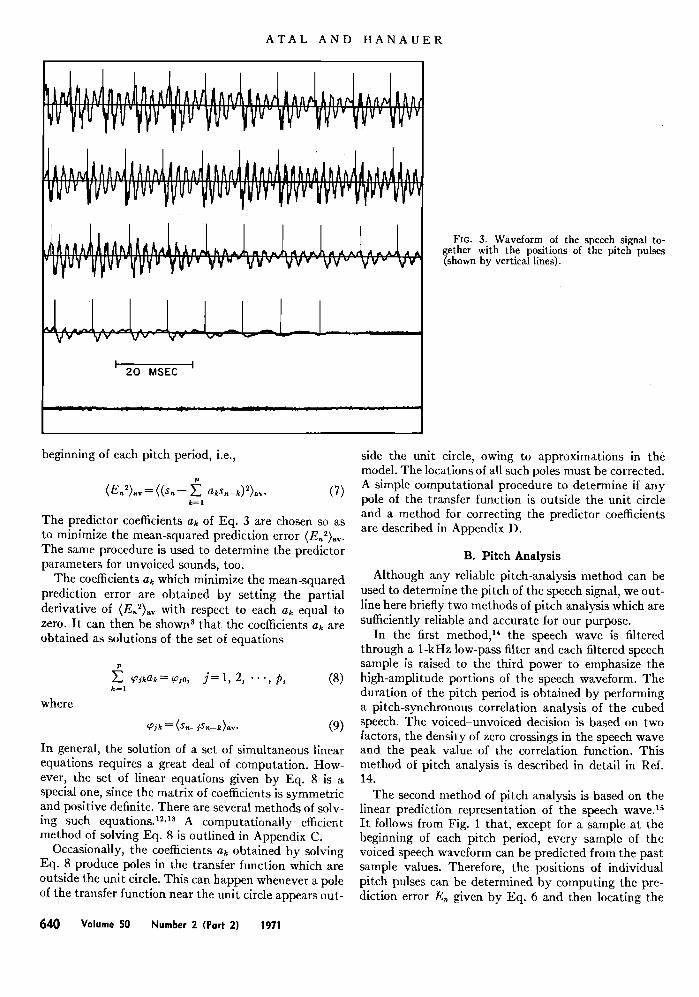
FIo. 5. Variation ot the minimum value of the rms prediction error with p, the number of predictor coefficients. Solid line shows the curve for voiced speech. Dotted line shows the curve for unvoiced speech.

From Eq. 3, the impulse response of the linear recursive filter of Fig. 1 satisfies the equation

s,.= • a•s._•, n> 1, (10)

with the initial conditions So= 1 and s, =0 for n<0. The autocorrelation function of the impulse response is, by definition, given by

r•il = • s,•s,•+14. (11)

Let us multiply both sides of Eq. 10 by s•+• and perform a sum over n from 0 to oo. We then obtain

and

ri= 5' anrfi_}f, i> 1, (12) k I

to= • a•r•q-l. (13)

Equations 12 and 13 enable us to compute the stunpies of the a•tocorrelation function from the predictor coefficients, and the predictor coefficients from the autocorrelation function. A computational procedure for performing the above operations is outlined in Appendix E.

The gain of the amplifier G is adjusted to provide the correct power in the synthesized speech signal. In any speech segment, the amplitude of the nth synthesized speech sample s• can be decomposed into two parts: one

part q• contributed by the memory of the linear predictor carried over from the previous speech segments and the other part v, contributed by the excitation from the current speech segment. Thus, s•=q,-{-v• =q•q-gu,, where g is the gain of the amplifier G. Let us assume that n = 1 is the first sample and n = M the last sample of the current speech segment. The first part q, is given by

q,= • a•q•_•, l<n<M, (14)

where qo, q-•, '", q•-v represent the memory of the predictor carried over from the previous synthesized speech segments. In addition, u• is given by

u•= 5•. a•u•_•+e•, l<n<M, (15)

where u•=0 for nonpositive values of n, and e• is the nth sample at the output of the voiced-unvoiced switch as shown in Fig. 4. Let P, be the mean-squared value of the speech samples. Then P, is given by

1

P, =-- • (q•-kgu,) •= (q•-k-gu•) •. (16)

On further rearrangement of terms, Eq. 16 is rewritten as

g•u•q - 2gq,u • Jrq,, • -- P, = O. (I 7 )

Equation 17 is solved for g such that g is real and non-


SPEECH ANALYSIS AND

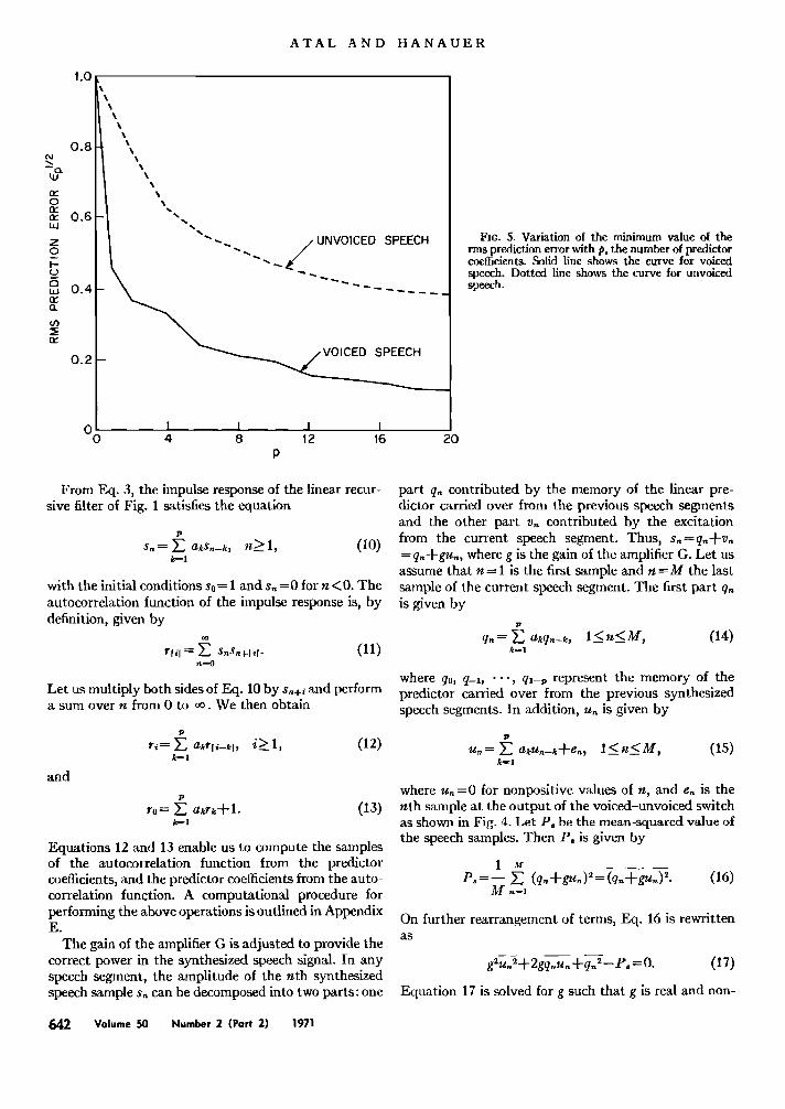
_FIG. 6. Comparison o[ wide-band sound spectrograms for synthetic and original speech signals for the utterance "May we all learn a yellow lion roar," spoken by a male speaker: (a) synthetic speech, and (b) original speech.

4

SYNTHESIS BY LINEAR PREDICTION

SYNTHETIC SPEECH

ORIGINAL SPEECH

0.5 1.5 2.0

I

TIME (SECONDS)

negative. In case such a solution does not exist, g is set to zero. The nth sample of the synthesized wave is finally obtained by adding q,, to gu,,.

IV. COMPUTER SIMULATION OF THE

ANALYSIS-SYNTHESIS SYSTEM

In order to assess the subjective quality of the synthesized speech, the speech analysis and synthesis system described above was simulated on a digital computer. The speech wave was first low-pass filtered to 5 kHz and then sampled at a frequency of 10 kHz. The analysis segment was set equal to a pitch period for voiced speech and equal to 10 msec for unvoiced speech. The various parameters were then determined for each analysis segment according to the procedure described in Sec. I I. These parameters were finally used to control the speech synthesizer shown in Fig. 4.

The optimum v,'due for the number of predictor parameters p was determined as follows: The speech wave was synthesized for various values of p between 2 and 18. Informal listening tests revealed no significant differences between synthetic speech samples for p larger than 12. There was slight degradation in speech qualit)- at p equal to 8. However, even for # as low as 2, the synthetic speech was intelligible althongh poor in qualit)-. The influence of decreasing p to values less than 10 was most noticeable on nasal consonants. Further-

more, the effect of decreasing p was less noticeable on female voices than on male voices. This could be ex-

pected in view of the fact that the length of the vocal tract for female speakers is generally shorter than for male speakers and that the nasal tract is slightly longer

than the oral tract. From these results, it was concluded that a wdue of p equal to 12 was required to provide an adequate representation of the speech signal. It may be worthwhile at this point to compare these results with the objective results based on an examination of the variation of the prediction error as a function of p. In Fig. 5, we have plotted the minimum value of the rms prediction error as a function of several values of p. The speech power in each case was normalized to unity. The results are presented separately for voiced and unvoiced speech. As can be seen in the figure, the prediction error crave is relatively flat for values of p greater than 12 for voiced speech and for p greater than 6 for unvoiced speech. These results suggest again that p equal to 12 is adequate for voiced speech. For unvoiced speech, a lower value of p, e.g., p equal to 6, should be adequate. For those readers who wish to listen to the quality of synthesized speech at various values of p, a recording accompanies this article. Appendix A gives the contents of the record. The reader should listen at this point to the first section of the record.

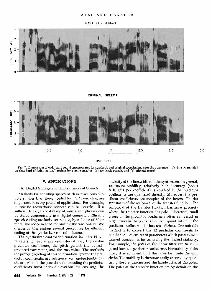
In informal listening tests, the qualit)- of the synthetic speech was found to be very close to that of the original speech for a wide range of speakers and spoken material. No significant differences were observed between the s•nthetic speech samples of male and female speakers. The second section of the record includes examples of synthesized speech for several utterances of different speakers. In each case, p was set to equal to 12. The spectrograms of the synthetic and the original speech for two of these utterances are compared in Figs. 6 and 7. As can be seen, the spectrogram of the synthetic speech closely resembles that of the original speech.


,I

'I 'l '" I

I I'

JJ' ,

•1111tl' , . ,'

ATAL AND HANAUER

SYNTHETIC SPEECH

i I

I

:11' ,

, Ih

ORIGINAL SPEECH

"I . I ! .

%0 t.5 2.O 2.5 3.O I I I I i

TIME (SEC)

Fro. 7. Comparison of wide-band sound spectrograms for synthetic and original speech signals for the utterance "It's time we rounded up that herd of Asian cattle," spoken by a male speaker: (a) synthetic speech, and (b) original speech.

V. APPLICATIONS

A. Digital Storage and Transmission of Speech

Methods for encoding speech at data rates considerably smaller than those needed for PCM encoding are important in many practical applications. For example, automatic answerhack services can be practical if a sufficiently large vocabulary of words and phrases can be stored economically in a digital computer. Efficient speech coding methods can rednee, by a factor of 30 or more, the space needed for storing the vocabulary. We discuss in this section several procedures for efficient coding of the synthesizer control information.

The synthesizer control information includes 15 parameters for every analysis interval, i.e., the twelve predictor coefficients, the pitch period, the voiced unvoiced parameter, and the rms value. The methods for proper encoding of this information, except the predictor coefficients, are relatively well nnderstood? On the other hand, the procedure for encoding the predictor coefficients must include provision for ensuring the

644 Volume 50 Number 2 (Port 2) 1971

stahility of the linear filter in the synthesizer. In general, to ensure stability, relatively high accuracy (about 8-10 bits per coefficient) is required if the predictor coefficients are quantized directly. Moreover, the predictor coefficients are samples of the inverse Fourier transform of the reciprocal of the transfer function. The reciprocal of the transfer function has zeros precisely where the transfer function has poles. Therefore, small errors in the predictor coefficients often can result in large errors in the poles. The direct quantization of the predictor coefficients is thus not efficient. One suitable method is to convert the 12 predictor coefficients to another equivalent set of parameters which possess well- defined constraints for achieving the desired stability. For example, the poles of the linear filter can be computed from the predictor coefficients. For stability of the filter, it is snfficient that the poles be inside the unit circle. The stability is therefore easily ensured by quantizing the frequencies and the bandwidths of the poles. The poles of the transfer function are by definition the


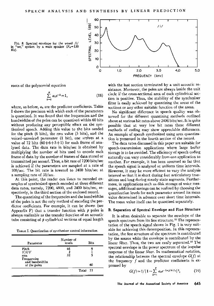
Fxo. 8. Spectral envelope for the vowel /i/ in "we," spoken by a male speaker (Fo=120 Hz).

• 60 5O

._1

"' 40

_1 •o

•: 20 I-

lO

I I I I I I I I I

/i/

I

1.0 2.0 3.0 4.0

FREQUENCY (kHz)

5.0

roots of the polynomial equation

Y•. akz-•= 1, (18) k•l

where, as before, a• are the predictor coefficients. Table I shows the precision with which each of the parameters is quantized. It was found that the frequencies and the bandwidths of the poles can be quantizod within 60 bits without producing any perceptible effect on the synthesized speech. Adding this value to the bits needed for the pitch (6 bits), the rms value (5 bits), and the voiced-unvoiced parameter (1 bit), one arrives at a value of 72 bits (60+6+5+1) for each frame of analyzed data. The data rate in bits/see is obtained by multiplying the number of bits used to encode each frame of data by the number of frames of data stored or transmitted per second. Thus, a bit rate of 7200 bits/see is achieved if the parameters are sampled at a rate of 100/sec. The bit rate is lowered to 2400 bits/see at a sampling rate of 33/sec.

At this point, the reader can listen to recorded examples of synthesized speech encoded at three different data rates, namely, 7200, 4800, and 2400 bits/see, respectively, in the third section of the enclosed record.

The quantizing of the frequencies and the bandwidths of the poles is not the only method of encoding the predictor coefficients. For example, it can be shown (see Appendix F) that a transfer function with p poles is always realizable as the transfer function of an acoustic tube consisting of p cylindrical sections of equal length

TABLE I. Quantization of synthesizer control information.

Number of Parameter levels Bits

Pitch 64 6 g/uv 2 1 rms 32 5 Frequencies

and bandwidths of the poles 60

Total 72

with the last section terminated by a unit acoustic resistance. Moreover, the poles are always inside the unit circle if the cross-sectional area of each cylindrical section is positive. Thus, the stability of the synthesizer filter is easily achieved by quantizing the areas of the sections or any other suitable function of the areas.

No significant difference in speech quality was observed for the different quantizing methods outlined above at various bit rates above 2400 bits/sec. It is quite possible that at very low bit rates these different methods of coding may show appreciable differences. An example of speech synthesized using area quantization is presented in the fourth section of the record.

The data rates discussed in this paper are suitable for speech-transmission applications where large buffer storage is to be avoided. The efficiency of speech coding naturally can vary considerably from one application to another. For example, it has been assumed so far that the speech signal is analyzed at uniform time intervals. However, it may be more efficient to vary the analysis interval so that it is short during fast articulatory tran- sitions and long during steady-state segments. Further- more, in applications such as disk storage of voice mes- sages, additional savings can be realized by choosing the quantization levels for each parameter around its mean value determined in advance over short time intervals. The mean value itself can be quantized separately.

B. Separation of Spectral Envelope and Fine Structure

It is often desirable to separate the envelope of the speech spectrum from its fine structure. ]s The representation of the speech signal shown in Fig. 1 is very suitable for achieving this decomposition. In this representation, the fine structure of the spectrum is contributed by the source while the envelope is contributed by the linear filter. ThuS, the two are easily separated? The spectral envelope is the power spectrum of the impulse response of the linear filter. In mathematical notation, the relationship between the spectral envelope G(f) at the frequency f and the predictor coefficients is expressed by

G(/)--1/I 1- E a*e-•'•Jz*'z'l ', (19)


ATAL AND HANAUER

60

• 5o 'El

-J •0 uJ

bJ

-J 30

bJ a_ •0 03

o o

I I I I I I . I I I

I I I I I I I I I i

1.o 2.0 3,0 4.0 5.0

FREQUENCY (kHz)

F[o. 9. Spectral envelope for the vowel /i/ in "we," spoken by a female speaker (F0--200 Hz).

where ak, as before, are the predictor coeffidents and f, is the sampling frequency. Two examples of the spectral envelope obtained in the above manner for the vowel /i/ belonging to the word "we" in the utterance "May we all learn a yellow lion roar" spoken by a male and a female speaker are illustrated in Figs. 8 and 9, respectively. We would like to add here that a spectral section obtained on a sound spectrograph failed to separate the third formant from the second formant for the female speaker both in the wide-band and the nar- row-band analysis. The spectral section showed one broad peak for the two formants. On the other hand, the spectral envelope of Fig. 9 shows the two formants without any ambiguity. Of course, it is difficult to evaluate the accuracy of this method from results based on real speech alone. Results with synthetic speech, where the spectral envelope is known precisely, indicate that the spectral envelope is accurately determined over a wide range of pitch values (from 50 to 300 Hz).

It also follows from Eq. 19 that, although the Fourier transform of G(J) is not time limited, the Fourier transform of I/G(/) is time limited to 2p/l, sec. Thus, spectral samples of G(/), spaced/s/2p Hz apart, are sufficient for reconstruction of the spectral envelope. For p=12 and f,=10 kHz, this means that a spacing of roughly 400 Hz between spectral samples is adequate.

In some applications, it may be desired to compute the Fourier transform of G(/), namely, the autocorrelation function. The autocorrelation function can be determined directly from the predictor coefficients without computing G(/). The relationship between the predictor coefficients and the autocorrelation function is given in Eqs. 12 and 13, and a computational method for performing these operations is outlined in Appendix E.

C. Formant Analysis

The objective of formant analysis is to determine the complex natural frequencies of the vocal tract as they change during speech production. If the vocal-tract configuration were known, these natural frequencies could be computed. However, the speech signal is in- fluenced both by the properties of the source and by the

vocal tract. For example, if the source spectrum has a zero close to one of the natural frequencies of the vocal tract, it will be extremely difficult, if not impossible, to determine the frequency or the bandwidth of that particular formant. A side-branch element such as the nasal

cavity creates a similar problem. In determining formant frequencies and bandwidths from the speech signal, one can at best hope to obtain such information which is not obscured or lost owing to the influence of the source.

Present methods of formant analysis usually start by transforming the speech signal into a short-time Fourier spectrum, and consequently suffer from many additional problems which are inherent in short-time Fourier transform techniques? o.2øa• Such problems, of course, can be completely avoided by determining the formant frequencies and bandwidths directly from the speech wave. 2

In the representation of the speech wave shown in Fig. 1, the linear filter represents the combined contributions of the vocal tract and the source to the spectral envelope. Thus, the poles of the transfer function of the filter include the poles of the vocal tract as well as the source. So far, we have made no attempt to separate these two contributions. For formant analysis, however, it is necessary that the poles of the vocal tract be separated out from the transfer function. In general, it is our experience that the poles contributed by the source either fall on the real axis in the unit circle or produce a relatively small peak in the spectral envelope. The magnitude of the spectral peak produced by a pole can easily be computed and compared with a threshold to determine whether a pole of the transfer function is indeed a natural frequency of the vocal tract. This is accomplished as follows:

From Eq. 4, the poles of the transfer function are the roots of the polynomial equation

• a•z-•= 1. (20)

Let there be n complex conjugate pairs of roots zt, z•*; z•, z2*; ß ß -; •, •*. The transfer function due to these

64• Volume 50 Number 2 (Port 2) 1971

SPEECH ANALYSIS AND

Fro. 10. Formant frequencies for the utterance "We were away a year ago," spoken by a male speaker (F0= 120 Hz). (a) Wide- band sound spectrogram for the above utterance, and (b) formants determined by the computer program.

4

0 o

SYNTHESIS BY LINEAR PREDICTION

WE WERE AWAY A YEAR AGO

.. u ;I [:

0.4 0.8 1.2

TIME (SEC)

(o)

o o 0.4 O.8 1.2 LG

TIME (SEC)

i

J

I

(b)

roots is given by

v½)=lrI (2]) i•l i•l

where the additional factors in the numerator set the transfer function at dc (•= 1) eqnal to 1. The specmd peak produced by the kth complex conjugate pole pair is given by

;1• (1-•)(1-•*) : l(7--zr,)(z--z•*-•-• I"' (22) where z = exp(2•rjf•T), a• = [ z•[ exp(2•rjf•T), and T is the sampling intervalß The threshold value of A} was set equal to 1.7. Finally, the formant frequency F• and

the bandwidth (two-sided root zu by

and

B• are related to the z-plane

F• = (1/2•rT) Im(lnz•), (23)

(') B• = (l/•rT) Re -- . lnz,,,

(24)

Examples of the formant frequencies determined according to the above procedure are illustrated in Figs. 10-12. Each figure consists of (a) a wide-band sonnd spectrogram of the utterance, and (b) formant data as determined by the above method. The results are presented for three different utterances. The first utterance, "We were away a year ago," was spoken by a male speaker (average fundamental frequency F0= 120 Hz).


ATAL AND HANAUER

MAY WE ALL LEARN A YELLOW LION ROAR

J ,( {

4

o o

0.5 t.o

TIME (SEC)

(o)

- 7 .', . ß ':: ' ß ..

ß .. : : ':. . ".. % :

0.5 t.0 1.5 2.0

TIME

2.0

Fro. ll. Formant frequencies for the utterance "May we all learn a yellow lion roar," spoken by a female speaker (Fo = 200 Hz). (a) Wide-band sound spectrogram for the above utterance, and (b) formants determined by the computer program.

(b)

The second utterance, "May we all learn a yellow lion roar," was spoken by a female speaker (F0=200 Hz). The third utterance, "Why do I owe you a letter?" was spoken by a male speaker (F0 = 125 Hz). Each point in these plots represents the results from a single frame of the speech signal which was equal to a pitch period in Figsß 10 and 11 and eqnal to 10 msec in Fig. 12. No

T•n,•E II. Factor by which each parameter was scaled for simulating a female voice from parameters derived from a male voiceß

Parameter Scaling factor

Pitch period T 0.58 Formant frequencies Fi 1.14 Formant bandwidths B, 2--Fi/5000


smoothing of the formant data over adjacent frames was done.

Again, in order to obtain a better estimate of the accuracy of this method of formant analysis, speech was synthesized with a known formant structure. The cor- respondence between the actual formant frequencies and bandwidths and the computed ones was found to be extremely close.

D. Re-forming the Speech Signals

The ability to modify the acoustical characteristics of a speech signal without degrading its quality is important for a wide variety of applications. For example, information regarding the relative importance of various acoustic variables in speech perception can be obtained by listening to speech in which some particular

SPEECH ANALVS1S AND SYNTHESIS BY LINEAR PIkEDICTION

WHY DO I OWE YOU A LETTER

Fro. 12. Formant frequencies for the utterance "Why do I owe you a letter?" spoken by a male speaker (Fo= 125 Hz). (a) Wide-band sound spectrogram for the above utterance, and (b) formants determined 1)y the computer program.

I

o o

i i i i

(a)

2

0 0.4 0.8

TIME (SFC.)

(b)

acoustic variables have been altered in a controlled

manner. The speech analysis and synthesis lechniques described in this paper can be used as a ttexible and convenient method for condncting snch speech-perception experiments. We wonld like to point oul here that the synthesis procedure allows independent control of such speech characteristics as spectral envdope, relative durations, pitch, and intensity. Thus, the speaking rate of a given speech signal may be ahered, e.g., for producing fast speech for blind persons or for producing slow speech for learning foreign languages. Or, in an application such as the recovery of "hdium speech," lhe frequencies of the spectral envelope can be scaled, leaving the fundamental frequency unchanged. Moreover, in

synthesizing seutence-length utterances from stored data about individual words, the method can be used to reshape the intonation and stress contours so that the speech sounds natural.

Iœxamples of speech in which selected acoustical characteristics have been altered are presented in the fifth section of the enclosed record. First, the listener can hear the utterance at the normal speaking rate. Next, the speaking rate is increased by a factor of 1.5. As the third item, the same utterance with the speaking rate reduced by a factor of 1.5 is presented. Finally, an example of a speech signal in which the pitch, the formant frequencies, and their bandwidths were changed from their original values, obtained from a male voice, to


ATAL AND HANAUER

TABLE III. Computation times needed to perform various operations discussed in the paper on the GE 635 (p = 10, fa = 10 kHz).

Operation Computation time Predictor coefficients

from speech samples (No. of samples = 100)

Spectral envelope (500 spectral samples) from predictor coefficients

Formant frequencies and bandwidths from predictor coefficients

p samples of autocorrelation function from predictor coefficients

Speech from predictor coefficients

Pitch analysis

75 msec/frame

250 msec/frame

60 msec/frame

t0 msec/frame

8 times real time 10 times real time

simulate a "female" voice is presented. The factor by which each parameter was changed from its original value is shown in Table II.

VI. COMPUTATIONAL EFFICIENCY

The computation times needed to perform several of the operations described in this paper are summarized in Table III. The programs were run on a GE 635 computer having a cycle time of 1 •sec. As can be seen, this method of speech analysis and synthesis is computationally efficient. In fact, the techniques are about five to 10 times faster than the ones needed to perform equivalent operations by fast-Fourier-transform methods. For instance, both the formant frequencies and their bandwidths are determined in 135 msec for each frame of the

speech wave 10 msec long. Assuming that the formants are analyzed once every 10 msec, the program will run in about 13 times real time; by comparison, fast-Fourier- transform techniques need about 100 times real time. Even for computing the spectral envelope, the method based on predictor coefficients is at least three times faster than the fast-Fourier-transform methods. The

complete analysis and synthesis procedure was found to run in approximately 25 times real time. Real-time operation could easily be achieved by using special hard- ware to perform some of the functions.

VII. CONCLUSIONS

We have presented a method for automatic analysis and synthesis of speech signals by representing them in terms of time-varying parameters related to the transfer function of the vocal tract and the characteristics of the

excitation. An important property of the speech wave, namely, its linear predictability, forms the basis of both the analysis and synthesis procedures. Unlike past speech analysis methods based on Fourier analysis, the method described here derives the speech parameters from a direct analysis of the speech wave. Consequently, various problems encountered when Fourier analysis is

applied to nonstationary and quasiperiodic signals like speech are avoided. One of the main advantages of this method is that the analysis procedure requires only a short segment of the speech wave to yield accurate results. This method is therefore very suitable for follow- ing rapidly changing speech events. It is also suitable for analyzing the speech of speakers with high-pitched voices, such as women or children. As an additional advantage, the analyzed parameters are rigorously related to other well-known speech characteristics. Thus, by first representing the speech signal in terms of the predictor coefficients, other speech characteristics can be determined as desired without much additional

computation. The speech signal is synthesized by a single recursive

filter. The synthesizer, thus, does not require any information about the individual formants and the for-

mants need not be determined explicitly during analysis. Moreover, the synthesizer makes use of the formant bandwidths of real speech, in contrast to formant syn- thesizers, which use fixed bandwidths for each formant. Informal listening tests show very little or no perceptible degradation in the quality of the synthesized speech. These results suggest that the analyzed parameters retain all the perceptually important features of the speech signal. Furthermore, the various parameters used for the synthesis can be encoded efficiently. It was found possible to reduce the data rate to approximately 2400 bits/sec without producing significant degradation in the speech quality. The above bit rate is smaller by a factor of about 30 than that for direct PCM encoding of the speech waveform. The latter bit rate is approximately 70 000 bits (70 000 bits = 7 bits/sampleX 10 000 samples/sec).

In addition to providing an efficient and accurate description of the speech signal, the method is computationally very fast. The entire analysis and synthesis procedure runs at about 25 times real time on a GE 635 digital computer. The method is thus well suited for analyzing large amounts of speech data automatically on the computer.

APPENDIX A: DESCRIPTION OF ENCLOSED RECORDED MATERIAL

Side 1

Section 1. Speech analysis and synthesis for various values of p, the number of predictor coefficients:

(a) p=2, (b) p=6, (c) p = 10, (d) p= 14, (e) p= 18, (f) original speech.

Section 2. Comparison of synthesized speech with the original, p= 12. Synthetic--original. Five utterances.



Section 3. Synthesized speech encoded at different bit rates, the parameters quantized as shown in Table I, p=12. Original--unquantized--7200 bits/sec--4800 bits/sec--2400 bits/sec. Three utterances.

Section 4. Synthesized speech obtained by quantizing the areas of an acoustic tube, p=12. Bit rate=7200 bits/sec.

(1) Frequencies and bandwidths quantized into 60-bit frames.

(2) Areas quantized into 60-bit frames.

The rest of the parameters are quantized as shown in Table I.

Section 5. Fast and slow speech, p= 14:

(a) Original speech. (b) Speaking rate = 1.5 times the original. (c) Speaking rate=0.67 times the original.

Section 6. Manipulation of pitch, formant frequencies, and their bandwidths, p= 10:

(a) Pitch, formant frequencies, and bandwidths altered as shown in Table II.

(b) Original voice.

APPENDIX B: RELATIONSHIP BETWEEN THE

LENGTH OF THE VOCAL TRACT AND THE NUMBER OF PREDICTOR COEFFICIENTS

Below about 5000 Hz, the acoustic properties of the vocal tract can be determined by considering it as an acoustic tube of variable cross-sectional area. The

relationship between sound pressure P, and volume velocity Uo at the glottis and the corresponding quan- tities P,, U, at the lips is best described in terms of the ABCD matrix parameters (chain matrix) of the acoustic tube. These parameters are defined by the matrix equation (see Fig. B-I):

qr,l

We now prove that the inverse Fourier transforms of these parameters in the time domain have finite duration r = 21/c, where l is the length of the tube and c is the velocity of sound. Let S(x) be the area function of the vocal tract, where x is the distance from the glottis to the point at which the cross-sectional area is specified. Consider a small element of tube of length dx at a distance x from the glottis. The ABCD matrix parameters of the tube element dx are given by m

A = D = cosh Fdx = 1/2(e r•+e-

B = --Z0 sinhPdx = --Zo(erax--e-ra•)/2, (B2)

C = -- sinh rdx/Zo = -- (e ra• _ e- r d-•)/2Zo,

where Z0 is the characteristic impedance of the tube element dx=oc/S(x), P is the propagation constant =jco/c, p is the density of air, c is the velocity of sound, and w is the angular frequency in radians. The ABCD matrix of the complete tube is given by the product of the ABCD matrices of the individual tube elements of

length dx spaced dx apart along the length of the tube. Let l=ndx. It is now easily verified that each of the ABCD parameters of the tube can be expressed as a power series in e ra• of the form

• olke kFdx.

The ABCD parameters are thus Fourier transforms of functions of time each with duration r=2n.dx/½. Taking the limit as dx--•O, n--}o•, and n.dx=l, we obtain r = 21/c.

From Eq. B1, the relationship between the glottal and the lip volume velocities is expressed in terms of the ABCD parameters by

Uo=CP,+DU•. (B3)

Since Pt•fioKUt, K being a constant related to the mouth area, Eq. B3 is rewritten as

U •-----(jco KC + D) U,. (B4)

Fro. B-I. Nonuniform acoustic tube.

GLOTTIS

P0,Ug

ß --.1•.!.:1-,-- d x {•[I [4'1

x LIPS

DISTANCE FROM GLOTTIS


ATAL AND HANAUER

The memory of the linear predictor (see Fig. 1) is by definition equal to the duration of the inverse Fourier transform of the reciprocal of the transfer function between the lip and the glottM volume velocities. There- fore, from Eq. B4, the memory of the linear predictor is equal to r--21/c.

APPENDIX C: DETERMINATION OF THE

PREDICTOR PARAMETERS FROM THE COVARIANCE MATRIX ß

Equation 8 can be written in matrix notation as

4,a = ½, (C1)

where •=[(qo•i)-I is a positive definite (or positive semidefinite) symmetric matrix, and a=l-(ai)-I and 4 = [(;oi0)] are column vectors. Since ß is positive definite (or semidefinite) and symtnetric, it can be expressed as the product of a triangular matrix V with real elements and its transpose V t . Thus,

4, = V V'. (C2)

Equation C1 can now be resolved into two simpler equations:

Vx = t•, (C3)

V'a =x. (C4)

Since V is a triangular matrix, Eqs. C$ and C4 can be solved recursively. m

Equations C3 and C4 provide a simple method of computing the minimum value of the prediction error (E•2),v as a function of p, the number of predictor coefficients. It is easily verified from Eqs. 7-9 that the minimum value of the mean-squared prediction error is given by

•p= •00-a% (C5)

On substituting for a from Eq. C4 into Eq. C5, we obtain

• = •00--x t V -• •,

which on substitution from Eq. C3 for • yields

• = •Ooo-X•. (C6)

Thus, the minimum value of the mean-squared prediction error is given as

q,= •,00- • x•. (C7) k 1

The advaxttage of using Eq. C7 lies in the fact that a single computation of the vector x for one value of p is sufficient. After the vector x is determined for the largest value of p at which the error is desired, % is calculated for smaller values of p from Eq. C7.

APPENDIX D: CORRECTION OF THE

PREDICTOR COEFFICIENTS

Let us denote by f(z) a polynomial defined by

J(z) =zV--a•z v-• ..... a•,, (DI)

where the polynomial coefficients a& are the predictor coefficients of Eq. 3. Associated with the polynomial f(z), we define a reciprocal polynomial ]*(z) by

f*(Z) -- -•-a•z•-• ..... •.• 1.

Let us construct the sequence of polynomials f•_•(z), f•_2(•), ..., f,(z), .- -, f•(z), where f=(s) is a polynomial of degree n, according to the formula

f,,(z) =k,,+,f=+,*(z) --l,,•_lfn+t(z), (D3)

where f•(z)=if(z), k• is the coefficient of z '• in f,(z), and l• is the constant term in f•(z). It can then be shown that the polynomial f(z) has all its zeros inside the unit circle if and only if I I•l > I k, I for each n_<p. D1

When one or more of the zeros of f(•) are outside the unit circle, let us set

f(z) = 1'I (s--z&). (D4) k 1

For every k for which [ z• I > 1, we replace z• by z•/I z• [ in Eq. D4 and construct a new polynonfial which has all of its zeros either inside or on the unit circle.

The above procedure is also suitable for testing that all the zeros of f(z) are within any given circle I zl =r. In this case, we replace a• by r-aa, in Eq. D1 and proceed as before.

The roots of the polynomial f(s) are determined by an iterative procedure based on the Newton Raphson method. m We start with a trial value of the root and

then construct successively better approximations. The iteration formula has the form

f[•"•] gk ("1) =Jgi (a) (DS)

where z•{• is the approximation of the/th root at the nth iteration. The iteration process is continued until either f(z)=0 or the absolute difference between the roots in two successive iterations is less than a fixed

threshold value. If convergence is not reached within lO0 iterations, a new starting value is selected. The starting value is chosen randomly on the unit circle. Furthermore, the starting value never lies on the real axis.

APPENDIX E: DETERMINATION OF THE PRE-

DICTOR COEFFICIENTS FROM THE AUTO-

CORRELATION FUNCTION AND THE

AUTOCORRELATION FUNCTION FROM

THE PREDICTOR COEFFICIENTS

We outline first a method of solving Eq. 12 for the predictor coefficients. Consider the set of equations

r,.=ka•)r!i_&t, for n>i>l. (El)

652 Volume 50 Number 2 (Port 2) 19'/I


Equation E1 is identical to Eq. 12 for n=p. In matrix form the above equation becomes

•'1 F 0 ß ß ß Fn_9 0•2 (n)

i, : i i = . (E2) [r•_x r• .-. r0 [ a?) J

Let R• be the nXn matrix on the left side of Eq. E2, a• <•) an m-dimensional vector whose kth component is a• (•>, and r• an n-dimensional vector whose kth com- •nent is r•_•. Let us define, for every vector, a reciprocal vector by the relationship

a•(•)*[ •=a•r•) [ •-•+x. (E3)

Equation E2 can now be rewritten as

R,.4a._x (") +a. (•')r._• = r,_x*, (E4)

r._•a._xr")+roa? ) =r.. (ES)

On multiplying Eq. E4 through by R,• -• and rearrang- ing terms, we obtain

a._• t") =R._ff•r._•*--a.(")R._ctr._•. (E6)

It is easily verified from Eq. E2 that

R._f•r._• * =a._• (•-•). (E7)

Inserting Eq. E7 into Eq. E6 gives

a._• (") =a._• ("-•) -- a?)[a._•("-o ] *. (E8)

Next, we multiply Eq. E8 through by r,-d and insert the result in Eq. E5. After rearrangement of the terms, we find that

n--I n--1

a?)[r0-E r•a•("-•)•=r. -- E r.-•a• (•-•). (E9) k•l

Equations E8 and E9 provide a complete recursire mlution of Eq. El. We start with n = 1. The solution is obviously

• •r•/ro. (El0)

Next, a• (•) and a•_• (•) are computed for successively increasing values of n until n=p. Furthermore, if R• is nonsingular, the expression inside the brackets on the left side of Eq. E9 is always positive. Therefore, a• (•) is always finite.

To determine the autocorrelation function from the

predictor coefficients, we proceed as follows: From Eq. E8,

[a•_•{•* = Ea•_•t•-"]*-a?•a•_•(•-< (Ell)

Therefore, after eliminating [a•_•(•-•)] * from Eqs. E8 and Ell, one obtains

Starting with n=p, we compute a? ) for successively smaller values of n until n=l. The autocorrelation

function at the nth sampling instant is given from Eq. E1 by

r,,=• a•(")r•,_k, for l_<n_<p. (El3) k=l

The samples of the autocorrelation function are computed recursively for successively larger values of n starting with n = 1. Note that, on the right side of Eq. El3, only samples up to r._• appear in the sum. Thus, r, can be computed recursively. Equation El3 is used to determine all the samples of the autocorrelation function with r0 normalized to 1. The value of r0 is finally determined from Eq. 13.

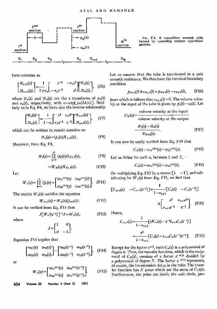
APPENDIX F: TRANSFER FUNCTION OF A NONUNIFORM ACOUSTIC TUBE

We consider sound transmission in an acoustic tube

formed by cascading N uniform cylindrical sections, each of length A as shown in Fig. F-1. Let the cross-sectional area of the nth section be S,. Let p,(t) and v,•(t) be the components of the volume velocity due to the forward- and the backward-traveling waves, respectively, at the input of the nth section. Let us assume that there is a sound source of constant volume

velocity at the input of the first section. Consider now the sound transmission between two adjacent sections, e.g., n and n+ 1. On applying the boundary conditions for the continuity of volume velocity and sound pressure across the junction, we obtain

A A

(F1)

=[p•+x(t)+v•+•(t)•----, (F2) Sn+l

where pc is the characteristic impedance of air. Equa- tions F1 and F2 can be solved for p,,+t(t) and v•+;(t). We then obtain

p.+fft) = Fp.(t---•-r.v•(t+--•l, (F3) l+r•L \ c l \ c l A

1 A A

1 +r. \ c / \ c/_1

where

S•--S.+• = -- (FS)

It is convenient to write Eqs. F3 and F4 in the z-trans-


ATAL AND HANAUER

section

2nd section

I Pn(t) I

Un(t)

SI $2 S3 Sn

i

•_ .... 1 Nth section

Sn+l $N

Fta. F-1. A nonuniform acoustic tube formed by cascading uniform cylindrical sectious.

form notation as

1 ' [ -• t , (F6) Lx•+t(,.)J- • +,•L-,•z-• z 3L•dz)J where •(z) and •(z) are the z transforms of and u,(t), respectively, with z=exp[j•(2•/•)]. Simi- larly as in Eq. F6, we have • the inverse relationship

f '"'IV • , (•7) whi• c•n be written in matrix notation •s

Mor•ver, •rom •q. FS,

:w•½)N•+,½). (•0) Let

•-• -Fwn(• )(z) w'2(")(z)]. (Fll) W•(z) = fi Qk(z) - Cw2• (>(z) The matrix IV,(,) satisfies the equation

W,+•(z) = W,(z)p,q4(z). (F12)

It can be verified from Eq. FI1 that

JEW,/(z-•)]-tJ = IV. (z), (F13) where

EquatiQn F13 implies that

w2,(z) w._(z)-I-Lwn(*'-9 or


Let us assume that the tube is terminated in a unit acoustic resistance. We then have the terminal boundary condition

p•r+t(t)-Futv+•(t) = p•+•(t) -u•t(/), (F16)

from which it follows that us+t(t) =0. The volume velocity at the input of the tube is given by pt(t)--•(t). Let

volume velocity at the input C•r(z)

volume velocity at the output

_ (F17) •t,-+,(z)

It can now be easily verified from Eq. F10 that

Cx,(z) =wn(m(z)--w2,(m(z). (F18)

Let us define for each n, between 1 and N, ß

C.(z) = wnt")(z) --w2•(")(z). (F19)

On multiplying Eq. F12 by a vector [1 --1], and substituting for W,(a) from Eq. F15, we find that

1

[c.+, (•.) - c.+t(,- ') ] = •[c. ½) - c. ½- ') ]

Xr %{1_, :an+ lg«l. (F20) Hence,

1

- --.[C, (z) --r.+tC.(z-')z-']. (F21) 1 --rn+l

Except for the factor a,n, each C,(a) is a polynomial of degree n. Thus, the transfer function, which is the reciprocal of C•(z), consists of a factor z -m2 divided by a polynomial of degree N. The factor z -m• represents, of course, the transmission delay in the tube. The transfer function has N poles which are the zeros of C•(z). Furthermore, the poles are inside the unit circle, pro-


vided that rn satisfies the condition TM

Ir,,I <Z, (F22)

which, together with Eq. F5, implies that

Sn>0, l<n<N. (F23)

We now show that every all-pole transfer function having poles inside the unit circle is always realizable, except for a constant multiplying factor and a delay, as the transfer function of an acoustic tube.

It follows from Eq. F20 that

C,(z) = [C,+ffz)+rn+.•C,,+,(z-1)]. (F24) l+r,+•

Furthermore, for each C•(z), the ratio of the coefficients of z -•/2 and z •t2 is r,. Given CN(z), one can compute C,(z) for successively decreasing values of n starting with n=N from Eq. F24. In each case, the coefficient r, is always defined as the ratio of the coefficients of z -n/: and z "/2. A sequence of numbers, r•, rz, ..., rN, obtained in the above manner, defines a tube with areas S•, S=, ß ß., S• according to Eq. FS, provided that each of the areas is positive, i.e., [r,[ <1 for l<n<N. This is, however, assured if the original polynomial CN(Z) has all its roots inside the unit circle (see Appendix D). Since the poles of the transfer function are inside the unit circle, it is indeed true.

•J. L. Flanagan, Speech Analysis Synthesis and Perception (Academic, New York, 1965), p. 119.

* E. N. Pinson, "Pitch-Synchronous Time-Domain Estimation of Formant Frequencies and Bandwidths," J. Acoust. Soc. Amer. 35, 1264-1273 (1963).

a B. S. Atal and M. R. Schroeder, "Adaptive Predictive Coding of Speech Signals," Bell System Tech. J. 49, 1973-1986 (1970).

4 B. S. Atal, "Speech Analysis and Synthesis by Linear Predic- tion of the Speech Wave," J. Acoust. Soc. Amer. 47, 65 (A) (1970).

[B. S. Atal, "Characterization of Speech Signals by Linear Prediction of the Speech Wave," Proc. IEEE Syrup. on Feature

Extraction and Selection in Pattern Recognition, Argonne, Ill. (Oct. 1970), pp. 202-209.

• M. V. Mathews, J. E. Miller, and E. E. David, Jr., "Pitch Synchronous Analysis of Voiced Sounds," J. Acoust. Soc. Amer. 33, 179-186 (1961).

? C. G. Bell, H. Fujisaki, J. M. Heinz, K. N. Stevens, and A. S. House, "Reduction of Speech Spectra by Analysis-by-Synthesis Techniques," J. Acoust. Soc. Amer. 33, 1725-1736 (1961).

e G. Fant, Acoustic Theory of Speech Production (Mouton, The Hague, 1960), p. 42.

• B. S. Atal, "Sound Transmission in the Vocal Tract with Applications to Speech Analysis and Synthesis," Proc. Int. Congr. Acoust., 7th, Budapest, Hungary (Aug. 1971).

•0 Each factor of the form (1-az -•) can be approximated by [1/(l+az-X+a•z'-:+...)] if Ja[<l, which is the case if the zeros are inside the unit circle.

n Ref. 1, p. 33. ta C. E. Fr0berg, Introduction to Numerical Analysis (Addison-

Wesley, Reading, Mass., 1969), 2nd ed., pp. 81-101. u j.p. Ellington and H. McCallion, "The Determination of

Control System Characteristics from a Transient Response," Proc. IEE 105, Part C, 370-373 (1958).

1• B. S. Atal, "Automatic Speaker Recognition Based on Pitch Contours," PhD thesis, Polytech. Inst. Brooklyn (1968).

xs B. S. Atal, "Pitch-Period Analysis by Inverse Filtering" (to be published).

• U. Grenander and G. Szeg6, Toeplltz Forms and Their Ap- plications (Univ. California Press, Berkeley, 1958), p. 40.

• L. G. Stead and R. C. Weston, "Sampling and Quantizing the Parameters of a Formant-Tracking Vocoder System," Proc. Speech Commun. Seminar, R.I.T., Stockholm (29 Aug.-1 Sept. 1962).

X•M. R. Schroeder, "Vocoders: Analysis and Synthesis of Speech," Proc. IEEE S4, 720-734 (1966).

l•The problem of separating the spectral envelope from the fine structure of the speech spectrum should be distinguished from the problem of separating the influence of the source from the speech spectrum. The latter problem is far more difficult and is discussed partially in the next subsection.

:• R. W. Schafer and L. R. Rabiner, "System for Automatic Formant Analysis of Voiced Speech," J. Acoust. Soc. Amer. 47, 634-648 (1970).

• J.P. Olive, "Automatic Formant Tracking by a Newton- Raphson Technique," J. Acoust. Soc. Amer. 50, 661-670 (1971).

mi. Malecki, Physical Foundations of Technical Acoustics, English transl. by I. Bellerr (Pergamon, Oxford, England, 1969), p. 475.

cx D. K. Faddeer and V. N. Faddeeva, Computational Methods of Linear Algebra, English transl. by R. C. Williams (W. H. Freeman, San Francisco, 1963), pp. 144-147.

m Ref. 16, pp. 4041. See also L. Ya. Geronimus, Orthogonal Polynomials (Consultants Bureau, New York, 1961), p. 156.

m Ref. 12, pp. 21-28.


Documents

Speech Analysis and Synthesis by Linear Prediction of …courses.cs.tamu.edu/rgutier/cpsc689_s07/atalHanauer1971lpc.pdf · Received 2 April 1971; revised 21 April 1971 9.8, 9.3 Speech