Spectrum Chapter Representation - eas.uccs.edumwickert/ece2610/lecture_notes/ece2610_chap3.pdfECE 2610 Signal and Systems 3–1 Spectrum Representation • Extending the investigation

er
Spectrum Representation• Extending the investigation of Chapter 2, we now consider
signals/waveforms that are composed of multiple sinusoidshaving different amplitudes, frequencies, and phases

(3.1)

where here is real, is complex, and is the frequency in Hz

• We desire a graphical representation of the parameters in(3.1) versus frequency

The Spectrum of a Sum of Sinusoids

• An alternative form of (3.1), which involves the use of theinverse Euler formula’s, is to expand each real cosine intotwo complex exponentials

(3.2)

x t A0 Ak 2fkt k+ cos

k 1=

N

+=

X0 Re Xkej2fkt

k 1=

N

+=

X0 A0= Xk Akejk= fk

x t X0

Xk2-----e

j2fkt Xk*

2------e

j– 2fkt+

k 1=

N

+=

Chapt

3

ECE 2610 Signal and Systems 3–1


– Note that we now have each real sinusoid expressed as asum of positive and negative frequency complex sinusoids

Two-Sided Sinusoidal Signal Spectrum: Express as in(3.2) and then the spectrum is the set of frequency/amplitudepairs

(3.3)

• The spectrum can be plotted as vertical lines along a fre-quency axis, with height being the magnitude of each orthe angle (phase), thus creating either a two-sided magnitudeor phase spectral plot, respectively

– The text first introduces this plot as a combination of mag-nitude and phase, but later uses distinct plots

Example: Constant + Two Real Sinusoids

(3.4)

• We expand into complex sinusoid pairs

(3.5)

x t

0 X0 f1 X1 2 f– 1 X1* 2

fk Xk 2 f– k Xk*

2

fN XN 2 f– N XN*

2

Xk

x t 5 3 2 50 t 8+ cos+=

6 2 300 t 2+ cos+

x t

x t 532---ej 250t

8---+

32---e

j– 250t 8---+

+ +=

62---ej 2300t

2---+

62---e

j– 2300t 2---+

+ +

ECE 2610 Signals and Systems 3–2


• The frequency pairs that define the two-sided line spectrumare

(3.6)

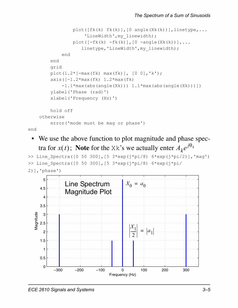
• We can now plot the magnitude phase spectra, in this casewith the help of a MATLAB custom function

function Line_Spectra(fk,Xk,mode,linetype)% Line_Spectra(fk,Xk,range,linetype)%% Plot Two-sided Line Spectra for Real Signals%----------------------------------------------------% fk = vector of real sinusoid frequencies% Xk = magnitude and phase at each positive frequency in fk% mode = 'mag' => a magnitude plot, 'phase' => a phase % plot in radians % linetype = line type per MATLAB definitions%% Mark Wickert, September 2006; modified February 2009 if nargin < 4 linetype = 'b';end my_linewidth = 2.0; switch lower(mode) % not case sensitive case {'mag','magnitude'} % two choices work k = 1; if fk(k) == 0 plot([fk(k) fk(k)],[0 abs(Xk(k))],linetype,... 'LineWidth',my_linewidth); hold on else Xk(k) = Xk(k)/2; plot([fk(k) fk(k)],[0 abs(Xk(k))],linetype,...

0 5 50 1.5ej 8 50– 1.5e

j– 8 ,

300 3ej 2 300 3e

j– 2 –



'LineWidth',my_linewidth); hold on plot([-fk(k) -fk(k)],[0 abs(Xk(k))],linetype,... 'LineWidth',my_linewidth); end for k=2:length(fk) if fk(k) == 0 plot([fk(k) fk(k)],[0 abs(Xk(k))],linetype,... 'LineWidth',my_linewidth); else Xk(k) = Xk(k)/2; plot([fk(k) fk(k)],[0 abs(Xk(k))],linetype,... 'LineWidth',my_linewidth); plot([-fk(k) -fk(k)],[0 abs(Xk(k))],linetype,... 'LineWidth',my_linewidth); end end grid axis([-1.2*max(fk) 1.2*max(fk) 0 1.05*max(abs(Xk))]) ylabel('Magnitude') xlabel('Frequency (Hz)') hold off case 'phase' k = 1; if fk(k) == 0 plot([fk(k) fk(k)],[0 angle(Xk(k))],linetype,... 'LineWidth',my_linewidth); hold on else plot([fk(k) fk(k)],[0 angle(Xk(k))],linetype,... 'LineWidth',my_linewidth); plot([-fk(k) -fk(k)],[0 -angle(Xk(k))],linetype,... 'LineWidth',my_linewidth); hold on end for k=2:length(fk) if fk(k) == 0 plot([fk(k) fk(k)],[0 angle(Xk(k))],linetype,... 'LineWidth',my_linewidth); else



plot([fk(k) fk(k)],[0 angle(Xk(k))],linetype,... 'LineWidth',my_linewidth); plot([-fk(k) -fk(k)],[0 -angle(Xk(k))],... linetype,'LineWidth',my_linewidth); end end grid plot(1.2*[-max(fk) max(fk)], [0 0],'k'); axis([-1.2*max(fk) 1.2*max(fk) -1.1*max(abs(angle(Xk))) 1.1*max(abs(angle(Xk)))]) ylabel('Phase (rad)') xlabel('Frequency (Hz)') hold off otherwise error('mode must be mag or phase')end

• We use the above function to plot magnitude and phase spec-tra for ; Note for the Xk’s we actually enter

>> Line_Spectra([0 50 300],[5 3*exp(j*pi/8) 6*exp(j*pi/2)],'mag')

>> Line_Spectra([0 50 300],[5 3*exp(j*pi/8) 6*exp(j*pi/

2)],'phase')

x t Akejk

−300 −200 −100 0 100 200 3000

0.5

1

1.5

2

2.5

3

3.5

4

4.5

5

Mag

nitu

de

Frequency (Hz)

Line SpectrumMagnitude Plot

X0 a0=

X1

2------ a1=



A Notation Change

• The conversion to frequency/amplitude pairs is a bit cumber-some since the factor of must be carried for all termsexcept , therefore the text advocates a more compact spec-tral form where replaces according to the rule

(3.7)

• We can then write more compactly the general expression for as

(3.8)

−300 −200 −100 0 100 200 300

−1.5

−1

−0.5

0

0.5

1

1.5P

hase

(ra

d)

Frequency (Hz)

Line SpectrumPhase Plot

X1 a1=

Xk 2X0

ak Xk

ak

X0, k 0=

12---Xk, k 0

=

x t

x t akej2fkt

k N–=

N

=


Beat Notes

• The new notations are overlaid in the previous example

• In some cases all of the frequencies in the above sum arerelated to a common or fundamental frequency, via integermultiplication

Beat Notes

• A special case that occurs when we have at least two sinu-soids present, is an audio/musical effect known as a beat note

• A beat note occurs when we hear the sum of two sinusoidsthat are very close in frequency, e.g.,

(3.9)

where and

• In this definition

(3.10)

we further assume that

Beat Note Spectrum

x t 2f1t cos 2f2t cos+=

f1 fc f–= f2 fc f+=

fc12--- f1 f2+ center frequency= =

f12--- f2 f1– deviation frequency= =

f fc«


Beat Notes

• Consider Line_Spectra([95 105],[1 1],'mag')

• Through the trig double angle formula, or by direct complexsinusoid expansion, we can write that

(3.11)

• If is small compared to , then appears to have aslowly varying envelope controlled by filled bythe rapidly varying sinusoid

−100 −50 0 50 1000

0.05

0.1

0.15

0.2

0.25

0.3

0.35

0.4

0.45

0.5

Mag

nitu

de

Frequency (Hz)

f1 95 Hz= f2 105 Hz=

fc 100 Hz= f 5 Hz=

x t 2f1t cos 2f2t cos+=

Re ej2 fc f– t

ej2 fc f+ t

+ =

Re ej2fct e

j2ft–ej2ft+ =

Re ej2fct 2 2ft cos

=

2 2ft 2fct coscos=

f fc x t 2ft cos

2fct cos


Beat Notes

Beat Note Waveform

• Consider Hz and Hz>> t = 0:1/(50*100):2/5;>> x = 2*cos(2*pi*5*t).*cos(2*pi*100*t);>> plot(t,x)>> grid>> xlabel('Time (s)')>> ylabel('Amplitude')

• As approaches zero, the envelope fluctuations becomeslower and slower, and the beat note becomes a steady tone/note; only a single frequency is heard and the line spectrumbecomes a single pair of lines at just

• With two musicians tuning their instruments, the process ofgetting is called in-tune

fc 100= f 5=

0 0.05 0.1 0.15 0.2 0.25 0.3 0.35 0.4−2

−1.5

−1

−0.5

0

0.5

1

1.5

2

Time (s)

Am

plitu

de

Envelope(red dash)

f

fc

f 0


Beat Notes

Multiplication of Sinusoids

• In the study of beat notes we indirectly encountered sinusoi-dal multiplication

• Formally we may be interested in

(3.12)

• Using trig identity 5 from the notes Chapter 2, we know that

(3.13)

• Using this result to expand (3.12) we have that

(3.14)

• In words, multiplying two sinusoids of different frequencyresults in two sinusoids, one at the sum frequency and one atthe difference frequency

• For the case where the frequencies are the same, we get

(3.15)

Amplitude Modulation

• Multiplying sinusoids also occurs in a fundamental radiocommunications modulation scheme known as amplitudemodulation (AM)

– Today AM broadcasting is mostly sports and talk radio

x t 2f1t 2f2t coscos=

coscos12--- + cos – cos+ =

x t 2f1t 2f2t coscos=

12--- 2 f1 f2– t cos 2 f1 f2+ t cos+ =

x t cos2

2f0t 12--- 1 2 2f0 t cos+ = =


Beat Notes

• To form an AM signal we let

(3.16)

where is a message or information bearing signal, isthe carrier frequency, and is the modulation index

• The spectral content of would be say, speech or music(typically low fidelity), such that is much greater that thehighest frequencies in

• If the envelope of never crosses through zero, andthe means to recover from at a receiver is greatlysimplified (so-called envelope detection)

>> t = 0:1/(50*100):2/5;>> x = (1+.5*cos(2*pi*5*t)).*cos(2*pi*100*t);>> plot(t,x)

x t Ac 1 m t + 2fct cos=

v t in text

m t fc0 1

m t fc

m t

1 x t m t x t

0 0.05 0.1 0.15 0.2 0.25 0.3 0.35 0.4−1.5

−1

−0.5

0

0.5

1

1.5

Time (s)

Am

plitu

de

AM Modulation with Ac = 1, = 0.5

f 5 Hz=

fc 100Hz=


Beat Notes

• The spectrum of an AM signal, for a single sinusoid,can be obtained by expanding as follows

(3.17)

• Continuing the AM example with and , wehave

(3.18)

>> Line_Spectra([95 100 105],[1/4 1 1/4],'mag')

m t x t

x t Ac 1 2ft cos+ 2fct cos=

Ac 2fct cos=

Ac

2--------- 2 fc f– t cos 2 fc f+ t cos+ +

Ac 1= 0.5=

x t 2100t cos=

14--- 2 95 t cos 2 105 t cos+ +

−100 −50 0 50 1000

0.05

0.1

0.15

0.2

0.25

0.3

0.35

0.4

0.45

0.5

Mag

nitu

de

Frequency (Hz)

AM Modulation Ampl. Spectra with Ac = 1, = 0.5

Carrier

Information bearingsidebands

95 105


Periodic Waveforms

Periodic Waveforms

• We have been talking about signals composed of multiplesinusoids, but until now we have not mentioned anythingabout these signals being periodic

• Recall that a signal is periodic if there exists some suchthat

– The smallest that satisfies this condition is the funda-mental period of

Example:

• Expanding we have

, (3.19)

which has component sinusoids at 2 Hz and 18 Hz

• The fundamental period is s, withHz being the fundamental frequency

• Since , we refer to the 18 Hz term as the 9th har-monic

• When a signal composed of multiple sinusoids is periodic,the component frequencies are integer multiples of the funda-mental frequency, i.e., , in the expression

(3.20)

• The fundamental frequency is the largest such that

T0x t T0+ x t =

T0x t

x t 2 28t cos 210t cos=

x t 218t cos 22t cos+=

T0 0.5=f0 1 T0 2= =

18 9 2=

fk kf0=

x t A0 Ak 2fkt k+ cosk 1=

N

+=

f0


Periodic Waveforms

, m an integer, , or in mathematicalterms the greatest common divisor

(3.21)

• In the example with and the largest divisorof {2,18} is 2, since 2/2 and 18/2 both result in integers, butthere is no larger value that works

Example: Suppose Hz

• The fundamental is Hz since 7 is a prime number

Nonperiodic Signals

• In the world of signal modeling both periodic and nonperi-odic signals are found

• In music, or least music that is properly tuned, periodic sig-nals are theoretically what we would expect

• It does not take much of a frequency deviation among thevarious components to make a periodic signal into a nonperi-odic signal

Example: Three Term Approximation to a Square Wave1

• This signal is composed of 1st, 3rd, and 5th harmonic com-ponents; fundamental is 100 Hz

1.More on this later in the chapter.

fk mf0= k 1 2 N =

f0 gcd fk = k 1 2 N =

f1 2= f2 18=

fk 3 7 9 =

f0 1=

xp t 2 100 t 13--- 2 300 t 1

5--- 2 500 t sin+sin+sin=


Periodic Waveforms

• We plot this waveform using MATLAB

>> t = 0:1/(50*500):0.1;>> x_per = sin(2*pi*100*t)+1/3*sin(2*pi*300*t)+...

1/5*sin(2*pi*500*t);>> strips(x_per,.1,50*500)>> xlabel('Time (s)')>> ylabel('Start Time of Each Strip')

• To make this signal nonperiodic we tweak the frequencies ofthe 3rd and 5th harmonics

>> x_nper = sin(2*pi*100*t)+...

0 0.01 0.02 0.03 0.04 0.05 0.06 0.07 0.08 0.09 0.1

0.4

0.3

0.2

0.1

0

Time (s)

Sta

rt T

ime

of E

ach

Str

ip

Clearly periodic

xnp t 2 100 t 13--- 2 89999 t sin+sin=

15---+ 2 249999 t sin


Periodic Waveforms

1/3*sin(2*pi*sqrt(89999)*t)+...1/5*sin(2*pi*sqrt(149999)*t);

>> strips(x_nper,.1,50*500)>> xlabel('Time (s)')>> ylabel('Start Time of Each Strip')

• It is interesting to note that the line spectra of both signals isvery similar, in particular the magnitude spectra as shownbelow

>> subplot(211)>> Line_Spectra([100 300 500],[1 1/3 1/5],'mag')>> subplot(212)>> Line_Spectra([100 sqrt(89999) sqrt(249999)],...

[1 1/3 1/5],'mag')

0 0.01 0.02 0.03 0.04 0.05 0.06 0.07 0.08 0.09 0.1

0.4

0.3

0.2

0.1

0

Time (s)

Sta

rt T

ime

of E

ach

Str

ip

No evidence of being periodic


Fourier Series

Fourier Series

Through the study of Fourier1 series we will learn how any peri-odic signal can be represented as a sum of harmonically relatedsinusoids.

• The synthesis formula is

(3.22)

where is the period

• The analysis formula will determine the from

1.French mathematician who wrote a thesis on this topic in 1807.

−600 −400 −200 0 200 400 6000

0.1

0.2

0.3

0.4

Mag

nitu

de

Frequency (Hz)

−600 −400 −200 0 200 400 6000

0.1

0.2

0.3

0.4

Mag

nitu

de

Frequency (Hz)89999 249999

300 500

x t akej 2 T0 kt

k –=

=

T0

ak x t


Fourier Series

• For a real signal, we see that andthen we can write that

(3.23)

Fourier Series: Analysis

• To obtain a Fourier series representation of periodic signal we need to evaluate the Fourier integral

(3.24)

where is the fundamental period

• As a special case note that the DC component of , givenby , is

(3.25)

– We call the average value since it finds the area under over one period divided (normalized) by

Fourier Series Derivation

• Since working with complex numbers is a relatively new con-cept, it might seem that proving (3.24) which involves com-plex exponentials, is out of reach for this course; not so

• The result of (3.24) can be established through a careful step-by-step process

x t a k– ak* conj ak = =

x t A0 Ak 2 T0 kt k+ cos

k 1=

+ Xk Akejk= =

x t

ak1T0----- x t e

j 2 T0 kt–td

0

T0

=

T0

x t a0

a01T0----- x t td

0

T0

=

a0x t T0


Fourier Series

• We begin with the property that integration of a complexexponential over an integer number of periods is identicallyzero, i.e.,

(3.26)

– Verify Version #1:

since for any integer

– Verify Version #2: Expand the integrand using Euler’s for-mula

since integrating over one or more complete cycles of sin/cos is always zero

• Regardless of the harmonic number k, all complex exponen-tials of the form , repeat withperiod , i.e.,

ej 2 T0 kt

td

0

T0

0=

ej 2 T0 kt

td0

T0

ej 2 T0 kt

j 2k T0 --------------------------

0

T0

ej 2 T0 kT0 1–j 2k T0

------------------------------------ 0= = =

ej2k

1= k 1 2 =

ej 2 T0 kt

td0

T0

2T0------ kt

j2T0------ kt

sin+cos

td0

T0

=

0 j0+ 0==

vk t j 2k T0 t exp=T0


Fourier Series

Orthogonality Property

(3.27)

– Note:

– Proof:

– When the exponent is zero and the integral reducesto

vk t T0+ ej

2kT0

--------- t T0+

=

ej

2kT0

--------- t

ej

2kT0

--------- T0

=

ej

2kT0

--------- t

ej2k

=

vk t =

1

vk t vl* t td

0

T0

0, k lT0, k l=

=

vl* t j 2l T0 t exp * j– 2l T0 t exp= =

vk t vl* t td

0

T0

ej

2T0

------ kt

ej–

2T0

------ lt

td0

T0

=

ej

2T0

------ k l– t

td0

T0

=

k l=


Fourier Series

– When , but rather some integer, say m, we have

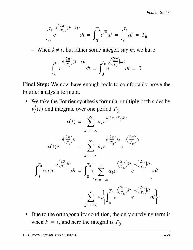
Final Step: We now have enough tools to comfortably prove theFourier analysis formula.

• We take the Fourier synthesis formula, multiply both sides by and integrate over one period

• Due to the orthogonality condition, the only surviving term iswhen , and here the integral is

ej

2T0

------ k l– t

td0

T0

ej0td

0

T0

td0

T0

T0= = =

k l

ej

2T0

------ k l– t

td0

T0

ej

2T0

------ mt

td0

T0

0= =

vl* t T0

x t akej 2 T0 kt

k –=

=

x t ej–

2T0

------ lt

akej

2T0

------ kt

ej–

2T0

------ lt

k –=

=

x t ej–

2T0

------ lt

td0

T0

akej

2T0

------ kt

ej–

2T0

------ lt

k –=

td0

T0

=

ak ej

2T0

------ kt

ej–

2T0

------ lt

td0

T0

k –=

=

k l= T0


Spectrum of the Fourier Series

• We are left with

or

and we have completed the proof!

Summary

(3.28)


• The spectrum associated with a Fourier series representationis consistent with the earlier discussion of two-sided linespectra

• The frequency/amplitude pairs are

(3.29)

x t ej–

2T0

------ lt

td0

T0

alT0=

al1T0----- x t e

j–2T0

------ lt

td0

T0

=

ak1T0----- x t e

j–2T0

------ kt

td0

T0

Analysis=

x t akej 2 T0 kt

k –=

Synthesis=

0 a0 f0 a 1 2f0 a 2 kf0 a k



Example:

• This signal has a Fourier series representation that we canobtain directly by expanding

• By comparing the above with the general Fourier series syn-thesis formula, we see that relative to Hz

x t cos2

2 1500 t =

cos2

cos2

2 1500 t ej21500t

ej– 21500t

+2

--------------------------------------------------

2

=

ej23000t

2 ej– 23000t

+ +4

----------------------------------------------------------- =

12---

14---ej23000t 1

4---e

j– 23000t+ +=

k 0= k 2= k 2–=Fourier Series Coeff.

f0 1 T0 1500= =

ak

1 2 , k 0=

1 4 , k 2=

0, otherwise

=

1/2

1/41/4

f (Hz)

3000-3000 0

Magnitude Spectrum f01T0----- 1500 Hz= =


Fourier Analysis of Periodic Signals


We can synthesize an approximation to some periodic oncewe have an expression for the Fourier coefficients using thefirst N harmonics

. (3.30)

• We can then implement the plotting of this approximationusing MATLAB

The Square Wave

• Here we consider a signal which over one period is given by

(3.31)

– This is actually called a 50% duty cycle square wave, sinceit is on for half of its period

x t ak

xN t akej 2 T0 kt

k N–=

N

=

s t 1, 0 t T0 2

0, T0 2 t T0

=

one periods t

0 T0T0

2------

1

a0 1 2=

3T0

2---------

T0

2------–

T– 0

t



• We solve for the Fourier coefficients via integration (the Fou-rier integral)

(3.32)

• Notice that , so

(3.33)

and for we have

(DC value) (3.34)

– This is the average value of the waveform, which is depen-dent upon the 50% aspect (i.e., halfway between 0 and 1)

• In summary,

(3.35)

ak1T0----- 1 e

j 2 T0 kt–td

0

T0 2

0+=

1T0----- e

j 2 T0 kt–

j 2 T0 k–-----------------------------

0

T0 2

1 ejk–

–j2k

--------------------==

ej–

1–=

ak1 1– k–j2k

----------------------= for k 0

k 0=

a01T0----- 1 e j0–

td0

T0 2

12---= =

ak

12--- , k 0=

1jk-------- , k 1 3 5 =

0, k 2 4 6 =

=



Spectrum for a Square Wave

• We can plot the square wave amplitude spectrum using theLine_Spectrum() function, by converting the coeffi-cients from back to

>> N = 15; k = 1:2:N; % odd frequencies>> Xk = 2./(j*pi*k); % Xk’s at odd freqs, Xk = 2*ak>> k = [0 k]; % augment with DC value>> Xk = [1/2 Xk]; % X0 = a0>> subplot(211)>> Line_Spectra(1*k,Xk,'mag')>> subplot(212)>> Line_Spectra(1*k,Xk,'phase')

ak Xk

−15 −10 −5 0 5 10 150

0.1

0.2

0.3

0.4

0.5

Mag

nitu

de

Frequency (Hz)

−15 −10 −5 0 5 10 15

−1

0

1

Pha

se (

rad)

Frequency (Hz)

f0 1 Hz=Square waveMagnitudeLine Spectra

Square wavePhaseLine Spectra

Only the odd harmonicspresent, i.e., k = 1, 3, 5, ..

......

...

...



Synthesis of a Square Wave

• We can synthesize a square wave by forming a partial sum,say up to the 15th harmonic; in (3.30)

• First we modify syn_sin() for Fourier series modelingfunction [x,t] = fs_synth(fk, ak, fs, dur, tstart)% [x,t] = fs_synth(fk, ak, fs, dur, tstart)%% Mark Wickert, September 2006 if nargin < 5, tstart = 0;end t = tstart:1/fs:dur;x = zeros(size(t));for k=1:length(fk) x = x + ak(k)*exp(j*2*pi*fk(k)*t);end

• The code used to produce simulation results for :>> N = 15; k = -N:2:N;>> ak = 1./(j*pi*k);>> fk = 1*[0 k];>> ak = [1/2 ak];>> [x,t] = fs_synth(fk, ak, 50*15, 3);>> plot(t,real(x)) % note x is not purely real>> grid % due to numerical imperfections>> xlabel('Time (s)')>> ylabel('Amplitude')

N 15=

x15 t



• With the approximation, we observe that there isringing or ears as the waveform makes discontinuous stepsfrom 0 to 1 and 1 back to 0

• This behavior is known as the Gibbs phenomenon, and comesabout due to the discontinuity of the ideal square wave

• The next plot shows that regardless of N, the ringing persistswith about a 9% overshoot/undershoot at the transition points

• The frequency of the rings increases as N increases>> N = 3; k = -N:2:N;>> ak = 1./(j*pi*k); ak = [1/2 ak];>> fk = 1*[0 k];>> [x3,t] = fs_synth(fk, ak, 50*15, 3);>> N = 7; k = -N:2:N;

0 0.5 1 1.5 2 2.5 3−0.2

0

0.2

0.4

0.6

0.8

1

1.2

Time (s)

Am

plitu

de

N 15=

f0 1 Hz=x15 t

N 15=



>> ak = 1./(j*pi*k); ak = [1/2 ak];>> fk = 1*[0 k];>> [x7,t] = fs_synth(fk, ak, 50*15, 3);>> N = 15; k = -N:2:N;>> ak = 1./(j*pi*k); ak = [1/2 ak];>> fk = 1*[0 k];>> [x15,t] = fs_synth(fk, ak, 50*15, 3);>> subplot(311); plot(t,real(x3))>> ylabel('x_3(t)')>> subplot(312); plot(t,real(x7))>> ylabel('x_7(t)')>> subplot(313); plot(t,real(x15))>> ylabel('x_15(t)')>> xlabel('Time (s)')

0 0.5 1 1.5 2 2.5 3−1

0

1

2

x 3(t)

0 0.5 1 1.5 2 2.5 3−1

0

1

2

x 7(t)

0 0.5 1 1.5 2 2.5 3−1

0

1

2

x 15(t

)

Time (s)

N 3=

N 7=

N 15=



• A limitation of Fourier series is that it cannot handle disconti-nuities very well, real physical waveforms do not have dis-continuities to the extreme found in mathematical models

Example: Frequency Tripler

• Suppose we have a sinusoidal signal

and we would like to obtain a sinusoidal signal of the form

• The systems aspect of this example is that we can convert into a square wave centered about zero, by passing the

signal through a limiter (like a comparator)

• The output signal is very similar to , that is

• The Fourier series coefficients of the square wave andthe square wave are related via an amplitude shifting andtime shifting property

• Without going into the details, it can be said that the coefficients for still only exist for k odd, and have ascale factor of the form

x t A 2f0t cos=

y t B 2 3f0 t cos=

x t

x t A 2f0t cos=

y t t

T0 1 f0=

1

-1

t1

-1

y t s t

y t 2s t T0 4+ 1–=

y t s t

ak k 0

C k



• Note that why?

• The Fourier coefficients that contribute to are at k = -3 and 3

• Knowing that the line spectra consists of all of the odd har-monics, means that in order to obtain just the 3rd harmonicwe need to design a filter that will allow just this signal topass (a bandpass filter)

• A system block diagram with waveforms and line spectra isshown below

Triangle Wave

• Another waveform of interest is the triangle wave

(3.36)

a0 0=

B 2 3f0 t cos

BandpassFilterat 3f0

f0f– 0

LineSpectra

3f03f– 0 3f03f– 0

f f f

t t t

x t y t xlim t

LineSpectra

LineSpectraRetain

This

1 12

3------Time

DomainTimeDomain

TimeDomain

Limiter

x t 2t T0 , 0 t T0 2

2 T0 t– T0 , T0 2 t T0

=



• We use the Fourier analysis formula to obtain the coef-ficients, starting with the DC term

(3.37)

• The remaining terms are found using integration

(3.38)

• To evaluate this integral we must use integration by parts, orfrom a mathematical handbook1 lookup the result that

1.Murray R. Spiegel, Mathematical Handbook of Formulas and Tables, 2nded., Schaum’s Outlines, McGraw Hill, New York, 1999.

one periodx t

0 T0T0

2------

1

a0 1 2=

3T0

2---------

T0

2------–

T– 0t

ak

a01T0----- x t td

0

T0

1T0----- area 1

T0-----

T0

2----- 1

2---= = = =

ak1T0----- 2t

T0-----

ej 2 T0 kt–

td0

T0 2

=

1T0-----

2 T0 t– T0

---------------------

ej 2 T0 kt–

tdT0 2

T0

+

xeaxxd e

ax

a------- x 1

a---–

=



• The symbolic engine of Mathematica can also solve this

• From the above Mathematica result, we note that and , so

(3.39)

since when k is odd and zero other-wise

Triangle Wave Spectrum

• Compare the line spectra for a triangle wave and square wave

I1 �1

T�Integrate�

2�t

T�Exp��

2 Π

T�k t�, �t, 0,

T

2��

�� k Π ��1 � �� k Π � � k Π�

2 k2 Π2

I2 �1

T�Integrate�

2��T � t�T

�Exp��2 Π

T�k t�, �t,

T

2, T��

��2 � k Π ��1 � �� k Π �1 � � k Π��2 k2 Π2

ak � FullSimplify�I1 � I2

�� k Π ��1 � Cos�k Π��

k2 Π2

ejk–

1– k= k cos 1– k=

ak1– k 1– k 1–

k22

----------------------------------------–

2

k22

----------- , k 1 3 5 =

1 2 , k 0=

0, k 2 4 6 =

= =

1– k 1– k 1– 2=



out to the 15th harmonic>> N = 15; k = 1:2:N;>> Xk = 2./(j*pi*k); Xk = [1/2 Xk];>> k = [0 k];>> subplot(211)>> Line_Spectra(1*k,Xk,'mag')>> N = 15; k = 1:2:N;>> Xk = -4./(pi^2*k.^2); Xk = [1/2 Xk];>> k = [0 k];>> subplot(212)>> Line_Spectra(1*k,Xk,'mag')

• Note that the spectral lines drop off with for the trian-gle wave, compared with just for the square wave

−15 −10 −5 0 5 10 150

0.1

0.2

0.3

0.4

0.5

Mag

nitu

de

Frequency (Hz)

−15 −10 −5 0 5 10 150

0.1

0.2

0.3

0.4

0.5

Mag

nitu

de

Frequency (Hz)

Square Wave

Triangle Wave

f0 1=

f0 1=

1 k2

1 k



• The relative smoothness of the triangle wave results in thefaster spectrum decrease

Synthesis of a Triangle Wave

• As with the square wave, we can synthesize size a trianglewave by forming a partial sum, say for

>> N = 3; k = -N:2:N;>> ak = -2./(pi^2*k.^2); ak = [1/2 ak];>> fk = 1*[0 k];>> [x3,t] = fs_synth(fk, ak, 50*15, 3);>> subplot(311); plot(t,real(x3)); grid>> ylabel('x_3(t)')>> N = 7; k = -N:2:N;>> ak = -2./(pi^2*k.^2); ak = [1/2 ak];>> fk = 1*[0 k];>> [x7,t] = fs_synth(fk, ak, 50*15, 3);>> subplot(312); plot(t,real(x7)); grid>> ylabel('x_7(t)')>> N = 15; k = -N:2:N;>> ak = -2./(pi^2*k.^2); ak = [1/2 ak];>> fk = 1*[0 k];>> [x15,t] = fs_synth(fk, ak, 50*15, 3);>> subplot(313); plot(t,real(x15))>> grid>> ylabel('x_{15}(t)'); xlabel('Time (s)')

• The triangle wave is continuous, so we expect the conver-gence of the partial sum to be much better than for thesquare wave

N 3 7 15 =

xN t



Convergence of Fourier Series

• For both the square wave and the triangle wave we have con-sidered synthesis via the approximation

• We know that the approximation is not perfect, in particularfor the square wave with the discontinuities, increasing N didnot seem to result in that much improvement

• We can define the error between the true signal and theapproximation , as

• The worst case error can be defined as

0 0.5 1 1.5 2 2.5 30

0.5

1x 3(t

)

0 0.5 1 1.5 2 2.5 30

0.5

1

x 7(t)

0 0.5 1 1.5 2 2.5 30

0.5

1

x 15(t

)

Time (s)

N 3=

N 7=

N 15=

f0 1=

xN t

x t xN t eN t x t xN t –=


Time–Frequency Spectrum

(3.40)

• We can then plot this for various N values

• For the square wave the maximum error is always 1/2 the sizeof the jump, and the overshoot, either side of the jump, isalways 9% of the jump


• The past modeling and analysis has dealt with signals havingparameters such as amplitude, frequency, and phase that donot change with time

• Most real world signals have parameters, such as frequency,that do change with time

Eworst maxt 0 T0

x t xN t –=

Square Wave Worst Case Error

9%

9%



• Speech and music are prime examples in our everyday life

Stepped Frequency

• A piano has 88 keys, with 12 keys per octave

– An octave corresponds to the doubling of pitch/frequency

– From one octave to the next there are 8 pitch steps, butthere are also half steps (flats and sharps)

• A constant frequency ratio is maintained between all notes

• The note A above middle C is at 440 Hz (tuning fork fre-quency) and is key number 49 of 88, so

• The C one octave above middle C is at key number 52, so

• A time-frequency plot can be used to display playing the

one octave

40 42 44 45 47 49 51 52

C4 D4 E4 F4 G4 A4 B4 C5Note Name

Note Number

r12

2= r 21 12

1.0595= =

fmiddle C fC4440 2

40 49– 12 261.6 Hz= =

fC5440 2

52 49– 12 523.3 Hz 2 261.6= =



notes in the C-major scale

Spectrogram Analysis

• The spectrogram is used to perform a time–frequency analy-sis on a signal, that is a plot of frequency content versus time,for a signal that has possibly time-varying frequencies

• When using MATLAB’s signal processing toolbox, the func-tion specgram() and spectrogram() are available forthis purpose

– The spfirst toolbox also has the function plotspec()

– Both specgram() and plotspec() plot frequency versustime, whereas spectrogram() plots time versus frequency

– The basic function interface to specgram() and plotspec is>> specgram(x,N_window,fsamp)>> plotspec(x,N_window,fsamp)

where N_window is the length of the spectrum analysiswindow, typically 256, 512, or 1024, depending upon thedesired frequency resolution and the rate at which the fre-quency content is changing

523 Hz494440392349330294262 Hz

TheoreticalTime-FrequencyPlot



Example: C–Major Scale

• The MATLAB function C_scale.m, given below, is used tocreate the C–major scale running from middle C to oneoctave above middle C

function [x,t] = C_scale(fs,note_dur)% [x,t_final] = C_scale()%% Mark Wickert % Generate octave middle Cpitch = [262 294 330 349 392 440 494 523];N_pitch = length(pitch); % Create a vector of frequenciesf = pitch(1)*ones(1,fix(note_dur*fs));for k=2:N_pitch f = [f pitch(k)*ones(1,fix(note_dur*fs))];endt = [0:length(f)-1]/fs;x = cos(2*pi*f.*t);

• We now call the function and plot the results using thespecgram function

>> [x,t] = C_scale(8000,.5);>> specgram(x,1024,8000);>> axis([0 4 0 1000]) % reduce the frquency axis



• In this example the note duration is 0.5 s

• There is also a large smear of spectral information seen as thescale progression steps from note-to-note

• This is due to the way the spectrogram is computed

– The analysis window straddles note changes, so a transientis captured where the pitch is jumping from one frequencyto the next

Time

Fre

quen

cy

0 0.5 1 1.5 2 2.5 3 3.5 40

100

200

300

400

500

600

700

800

900

1000

(s)

(Hz)


Frequency Modulation: Chirp Signals


In the previous example we have seen how a sinusoidal wave-form can have time varying frequency by stepping the frequency.Frequency modulation or angle modulation, provides anotherview on this subject within a particular mathematical framework.

Chirped or Linearly Swept Frequency

• A chirped signal is created when we sweep the frequency,according to some function, from a starting frequency to anending frequency

• A constant frequency sinusoid is of the form

(3.41)

• The argument of (3.41) is a time varying angle, , that iscomposed a linear term and a constant, i.e.,

(3.42)

• The units of is radians

• If we differentiate we obtain the instantaneous fre-quency

rad/s (3.43)

or by dividing by the instantaneous frequency in Hz

x t Re Aej 0t +

A 0t + cos= =

t

t 0t + 2f0t += =

t

t

i t d t dt

-------------- 0= =

2



Hz (3.44)

• The function can take on different forms, but in particu-lar it may be quadratic, i.e.,

rad (3.45)

which has corresponding instantaneous frequency

Hz (3.46)

• In this case we have a linear chirp, since the instantaneousfrequency varies linearly with time

Example: Chirping from 100 to 1000 Hz in 1 s

• The beginning and ending times are s and s

• We need to have

(3.47)

so

• Finally,

(3.48)

• The phase, , is

rad (3.49)

• We can implement this in MATLAB as follows:>> t = 0:1/8000:1;

fi t 1

2------d t

dt-------------- f0= =

t

t 2t2 2f0t + +=

fi t 2t f0+=

t1 0= t2 1=

fi 0 f0 100 Hz= =

fi 1 2 1 100+ 1000 Hz= =

900 2 450= =

fi t 900t 100 Hz 0 t 1 s +=

t

t 2 450t2 2 100t ++=



>> x = cos(2*pi*450*t.^2 + 2*pi*100*t + 2*pi*rand(1,1));>> plot(t,x)>> strips(x,.2,8000)>> xlabel('Time (s)')>> ylabel('Start Time of Each Strip (s)')

• Using the specgram function we can obtain the time–fre-quency relationship

>> specgram(x,512,8000);

0 0.01 0.02 0.03 0.04 0.05 0.06 0.07 0.08 0.09 0.1

0.9

0.8

0.7

0.6

0.5

0.4

0.3

0.2

0.1

0

Time (s)

Sta

rt T

ime

of E

ach

Str

ip (

s)

Linear Chirp from 100 Hz to 1000 Hz in 1 s


Summary

Summary

• The spectral representation of signals composed of sums ofsinusoids was the main focus of this chapter

• The two-sided line spectra is the means to graphically displaythe spectra

• The concept of fundamental period and frequency was intro-duced, along with harmonic number

• The Fourier series was found to be a power tool for both anal-ysis and synthesis of periodic signals

Time

Fre

quen

cy

0.1 0.2 0.3 0.4 0.5 0.6 0.7 0.8 0.90

500

1000

1500

2000

2500

3000

3500

4000

100

1000

(s)

(Hz)


Summary

• For sinusoids with time-varying parameters, in particular fre-quency, the spectrogram is a useful graphical display tool

• Stepped frequency signals, such as a scale being played on akeyboard, is particularly clear when viewed as a spectrogram

• Frequency modulation, in particular linear chirp signals werebriefly introduced


Documents

Spectrum Chapter Representation - eas.uccs.edumwickert/ece2610/lecture_notes/ece2610_chap3.pdfECE 2610 Signal and Systems 3–1 Spectrum Representation • Extending the investigation