HEWLETTPACKARD

Spectrum Analysis

Application Note 150

Spectrum AnalysisBasics

Application Note 150Spectrum Analysis Basics

@Hewlett-PackardCompany, 19741212 Valley House DriveRohnert Park, California, U.S.A.

All Rights Reserved. Reproduc-tion, adaptation, or translationwithout prior written permissionis prohibited, except as allowedunder the copyright laws.

November 1,1989

Hewlett-Packard Signal Analysis Division would like to acknowledgethe author, Blake Peterson, for more than 30 years of outstandingservice in engineering applications and technical education for HPand our customers.

Chapter 1 IntroductionWhat is a Spectrum?Why measure spectra?

112

Chapter 2 The Superheterodyne Spectrum AnalyzerTuning EquationResolutionAnalog FiltersDigital FiltersResidual FMPhase NoiseSweep TimeAnalog Resolution FiltersDigital Resolution FiltersEnvelope DetectorDisplay SmoothingVideo FilteringVideo AveragingAmplitude MeasurementsCRT DisplaysDigital DisplaysAmplitude AccuracyRelative UncertaintyAbsolute AccuracyImproving Overall UncertaintySensitivityNoise FigurePreamplifiersNoise as a SignalPreamplifier for Noise MeasurementsDynamic RangeDefinitionDynamic Range versus Internal DistortionAttenuator TestNoiseDynamic Range versus Measurement UncertaintyMixer CompressionDisplay Range and Measurement RangeFrequency MeasurementsSummaryFootnotes

4699

111212131314151616171818192121232324262731333434353838394041424445

Chapter 3 Extending the Frequency RangeHarmonic MixingAmplitude CalibrationPhase NoiseSignal IdentificationPreselectionImproved Dynamic RangeMultiband TuningPluses and Minuses of PreselectionWideband Fundamental MixingSummaryFootnotes

464649495052545656575959

Glossary of Terms 60Index 67

Chapter 1 Introduction

This application note is intended to serve as a primer on super-heterodyne spectrum analyzers. Such analyzers can also be de-scribed as frequency-selective, peak-responding voltmeters cali-brated to display the rms value of a sine wave. It is important tounderstand that the spectrum analyzer is not a power meter, al-though we normally use it to display power directly. But as long aswe know some value of a sine wave (for example, peak or average)and know the resistance across which we measure this value, wecan calibrate our voltmeter to indicate power.

What is a Spectrum?Before we get into the details of describing a spectrum analyzer, wemight first ask ourselves: just what is a spectrum and why wouldwe want to analyze it?

Our normal frame of reference is time. We note when certain eventsoccur. This holds for electrical events, and we can use an oscillo-scope to view the instantaneous value of a particular electricalevent (or some other event converted to volts through an appropri-ate transducer) as a function of time; that is, to view the waveformof a signal in the time domain.

Enter Fourier.’ He tells us that any time-domain electrical phe-nomenon is made up of one or more sine waves of appropriatefrequency, amplitude, and phase. Thus with proper filtering we candecompose the waveform of Figure 1 into separate sine waves, orspectral components, that we can then evaluate independently.Each sine wave is characterized by an amplitude and a phase. Inother words, we can transform a time-domain signal into its fre-quency-domain equivalent. In general, for RF and microwavesignals, preserving the phase information complicates this transfor-mation process without adding significantly to the value of theanalysis. Therefore, we are willing to do without the phase informa-tion. If the signal that we wish to analyze is periodic, as in our casehere, Fourier says that the constituent sine waves are separatedin the frequency domain by I/T, where T is the period of the signal.2

To properly make the transformation from the time to the fre-quency domain, the signal must be evaluated over all time, that is,over + infinity. However, we normally take a shorter, more practicalview and assume that signal behavior over several seconds orminutes is indicative of the overall characteristics of the signal.The transformation can also be made from the frequency to the timedomain, according to Fourier. This case requires the evaluation ofall spectral components over frequencies to + infinity, and the phaseof the individual components is indeed critical. For example, asquare wave transformed to the frequency domain and back againcould turn into a sawtooth wave if phase were not preserved.

1

So what is a spectrum in the context of this discussion? A collectionof sine waves that, when combined properly, produce the time-domain signal under examination. Figure 1 shows the waveform ofa complex signal. Suppose that we were hoping to see a sine wave.Although the waveform certainly shows us that the signal is not apure sinusoid, it does not give us a definitive indication of thereason why.

Figure 2 shows our complex signal in both the time and frequencydomains. The frequency-domain display plots the amplitude versusthe frequency of each sine wave in the spectrum. As shown, thespectrum in this case comprises just two sine waves. We now knowwhy our original waveform was not a pure sine wave. It contained asecond sine wave, the second harmonic in this case.

Are time-domain measurements out? Not at all. The time domain isbetter for many measurements, and some can be made only in thetime domain. For example, pure time-domain measurementsinclude pulse rise and fall times, overshoot, and ringing.

Why Measure Spectra?The frequency domain has its measurement strengths as well. We

have already seen in Figures 1 and 2 that the frequency domain isbetter for determining the harmonic content of a signal. Communi-cations people are extremely interested in harmonic distortion. Forexample, cellular radio systems must be checked for harmonics ofthe carrier signal that might interfere with other systems operatingat the same frequencies as the harmonics. Communications peopleare also interested in distortion of the message modulated onto acarrier. Third-order intermodulation (two tones of a complex signalmodulating each other) can be particularly troublesome because thedistortion components can fall within the band of interest and so

Fig. 2. Relationship betweentime and frequency domain

Time Domain Frequency DomainMeasurements Measurements

2

Spectral occupancy is another important frequency-domain meas-urement. Modulation on a signal spreads its spectrum, and toprevent interference with adjacent signals, regulatory agenciesrestrict the spectral bandwidth of various transmissions. Electro-magnetic interference (EMI) might also be considered a form ofspectral occupancy. Here the concern is that unwanted emissions,either radiated or conducted (through the power lines or otherinterconnecting wires), might impair the operation of other sys-tems. Almost anyone designing or manufacturing electrical orelectronic products must test for emission levels versus frequencyaccording to one regulation or another.

So frequency-domain measurements do indeed have their place.Figures 3 through 6 illustrate some of these measurements.

Fig. 3. Harmonic distortion teat. Fig. 4. Two-tone test on SSBtransmitter.

Fig. 6. Conducted emmissions plottedagainst ME limits as part of EMItest.

Fig. 6. Digital radio signal andmask showing limits of spectraloccupancy.

‘Jean Baptiste Joseph Fourier, 1768-1830, French mathematician and physicist.21f the time signal occurs only once, then T is infinite, and the frequency representa-tion is a continuum of sine waves:

3

Chapter 2The Superheterodyne Spectrum Analyzer

While we shall concentrate on the superheterodyne spectrumanalyzer in this note, there are several other spectrum analyzerarchitectures. Perhaps the most important non-superheterodynetype is that which digitizes the time-domain signal and thenperforms a Fast Fourier Transform (FFT) to display the signal inthe frequency domain. One advantage of the FFT approach is itsability to characterize single-shot phenomena. Another is thatphase as well as magnitude can be measured. However, at thepresent state of technology, FFT machines do have some limita-tions relative to the superheterodyne spectrum analyzer, particu-larly in the areas of frequency range, sensitivity, and dynamicrange.

Figure 7 is a simplified block diagram of a superheterodyne spec-trum analyzer. Heterodyne means to mix - that is, to translatefrequency - and super refers to super-audio frequencies, or frequen-cies above the audio range. Referring to the block diagram inFigure 7, we see that an input signal passes through a low-passfilter (later we shall see why the filter is here) to a mixer, where itmixes with a signal from the local oscillator (LO). Because themixer is a non-linear device, its output includes not only the twooriginal signals but also their harmonics and the sums and differ-ences of the original frequencies and their harmonics. If any of themixed signals falls within the passband of the intermediate-fre-quency (IF) filter, it is further processed (amplified and perhapslogged), essentially rectified by the envelope detector, digitized (inmost current analyzers), and applied to the vertical plates of acathode-ray tube (CRT) to produce a vertical deflection on the CRTscreen (the display). A ramp generator deflects the CRT beamhorizontally across the screen from left to right.* The ramp alsotunes the LO so that its frequency changes in proportion to theramp voltage.

LP IFFilter

I IMixer

Filter EnvelopeDetector

Fig. 7. Superheterodyne spectrumanalyzer.

RAMPGenerator

4

If you are familiar with superheterodyne AM radios, the type thatreceive ordinary AM broadcast signals, you will note a strongsimilarity between them and the block diagram of Figure 7. Thedifferences are that the output of a spectrum analyzer is the screenof a CRT instead of a speaker, and the local oscillator is tuned elec-tronically rather than purely by a front-panel knob.

Since the output of a spectrum analyzer is an X-Y display on a CRTscreen, let’s see what information we get from it. The display ismapped on a grid (graticule) with ten major horizontal divisionsand generally eight or ten major vertical divisions. The horizontalaxis is calibrated in frequency that increases linearly from left toright. Setting the frequency is usually a two-step process. First weadjust the frequency at the center line of the graticule with theCenter Frequency control. Then we adjust the frequency range(span) across the full ten divisions with the Frequency Span con-trol. These controls are independent, so if we change the centerfrequency, we do not alter the frequency span. Some spectrumanalyzers allow us to set the start and stop frequencies as analternative to setting center frequency and span. In either case, wecan determine the absolute frequency of any signal displayed andthe frequency difference between any two signals.

The vertical axis is calibrated in amplitude. Virtually all analyzersoffer the choice of a linear scale calibrated in volts or a logarithmicscale calibrated in dB. (Some analyzers also offer a linear scalecalibrated in units of power.) The log scale is used far more oftenthan the linear scale because the log scale has a much wider usablerange. The log scale allows signals as far apart in amplitude as 70to 100 dB (voltage ratios of 3100 to 100,000 and power ratios of10,000,000 to 10,000,000,000) to be displayed simultaneously. Onthe other hand, the linear scale is usable for signals differing by nomore than 20 to 30 dB (voltage ratios of 10 to 30). In either case, wegive the top line of the graticule, the reference level, an absolutevalue through calibration techniques2 and use the scaling perdivision to assign values to other locations on the graticule. So wecan measure either the absolute value of a signal or the amplitudedifference between any two signals.

In older spectrum analyzers, the reference level in the log modecould be calibrated in only one set of units. The standard set wasusually dBm (dB relative to 1 mW). Only by special request couldwe get our analyzer calibrated in dBmV or dBuV (dB relative to amillivolt or a microvolt, respectively). The linear scale was alwayscalibrated in volts. Today’s analyzers have internal microproces-sors, and they usually allow us to select any amplitude units (dBm,dBuV, dBmV, or volts) on either the log or the linear scale.

Scale calibration, both frequency and amplitude, is shown either bythe settings of physical switches on the front panel or by annotationwritten onto the display by a microprocessor. Figure 8 shows thedisplay of a typical microprocessor-controlled analyzer.

Fig. 8. Typical spectrum analyzerdisplay with control settings.

But now let’s turn our attention back to Figure 7.

5

Tuning EquationTo what frequency is the spectrum analyzer of Figure 7 tuned?That depends. Tuning is a function of the center frequency of theIF filter, the frequency range of the LO, and the range of frequen-cies allowed to reach the mixer from the outside world (allowed topass through the low-pass filter). Of all the products emerging fromthe mixer, the two with the greatest amplitudes and therefore themost desirable are those created from the sum of the LO and inputsignal and from the difference between the LO and input signal. Ifwe can arrange things so that the signal we wish to examine iseither above or below the LO frequency by the IF, one of thedesired mixing products will fall within the pass-band of the IFfilter and be detected to create a vertical deflection on the display.

How do we pick the LO frequency and the IF to create an analyzerwith the desired frequency range? Let us assume that we want atuning range from 0 to 2.9 GHz. What IF should we choose? Sup-pose we choose 1 GHz. Since this frequency is within our desiredtuning range, we could have an input signal at 1 GHz. And sincethe output of a mixer also includes the original input signals, aninput signal at 1 GHz would give us a constant output from themixer at the IF. The 1 GHz signal would thus pass through thesystem and give us a constant vertical deflection on the displayregardless of the tuning of the LO. The result would be a hole inthe frequency range at which we could not properly examinesignals because the display deflection would be independent of theLO.

So we shall choose instead an IF above the highest frequency towhich we wish to tune. In Hewlett-Packard spectrum analyzersthat tune to 2.9 GHz, the IF chosen is about 3.6 (or 3.9) GHz. Nowif we wish to tune from 0 Hz (actually from some low frequencybecause we cannot view a to O-Hz signal with this architecture) to2.9 GHz, over what range must the LO tune? If we start the LO atthe IF (LO - IF = 0) and tune it upward from there to 2.9 GHzabove the IF, we can cover the tuning range with the LO-minus-IFmixing product. Using this information, we can generate a tuningequation:

fBi, = f, - frr

where fmi, = signal frequency,f = local oscillator frequency, and!i = intermediate frequency (IF).

If we wanted to determine the LO frequency needed to tune theanalyzer to a low-, mid-, or high-frequency signal (say, 1 kHz, 1.5GHz, and 2.9 GHz), we would first restate the tuning equation interms of fLo:

fLO = fBi, + fW.

6

Then we would plug in the numbers for the signal and IF:

fL O

= 1 kHz + 3.6 GHz = 3.600001 GHz,f

L O= 1.5 GHz + 3.6 GHz = 5.1 GHz, and

fL O

= 2.9 GHz + 3.6 GHz = 6.5 GHz.

Figure 9 illustrates analyzer tuning. In the figure, fL, is not quitehigh enough to cause the f, - f+, mixing product to fall in the IFpassband, so there is no response on the display. If we adjust theramp generator to tune the LO higher, however, this mixingproduct will fall in the IF passband at some point on the ramp(sweep), and we shall see a response on the display.

Since the ramp generator controls both the horizontal position ofthe trace on the display and the LO frequency, we can now cali-brate the horizontal axis of the display in terms of input-signal fre-quency.

Freq Range-,- - -;’ of Analyzer ---- 1

1 Fig. 9. The LO must be tuned1I

to f, + fd. to produce a

Iresponse on the display.

II

f LO’f sig

'LO f

f LO+ f sig

We are not quite through with the tuning yet. What happens if thefrequency of the input signal is 8.2 GHz? As the LO tunes throughits 3.6-to-6.5-GHz range, it reaches a frequency (4.6 GHz) at whichit is the IF away from the 8.2-GHz signal, and once again we havea mixing product equal to the IF, creating a deflection on thedisplay. In other words, the tuning equation could just as easilyhave been

f,, = f, + f,.

This equation says that the architecture of Figure 7 could alsoresult in a tuning range from 7.2 to 10.1 GHz. But only if we allowsignals in that range to reach the mixer. The job of the low-passfilter in Figure 7 is to prevent these higher frequencies fromgetting to the mixer. We also want to keep signals at the inter-.mediate frequency itself from reaching the mixer, as described

7

above, so the low-pass filter must do a good job of attenuatingsignals at 3.6 GHz as well as in the range from 7.2 to 10.1 GHz.

In summary we can say that for a single-band RF spectrum ana-lyzer, we would choose an IF above the highest frequency of thetuning range, make the LO tunable from the IF to the IF plus theupper limit of the tuning range, and include a low-pass filter infront of the mixer that cuts off below the IF.

To separate closely spaced signals (see Resolution below), somespectrum analyzers have IF bandwidths as narrow as 1 kHz;others, 100 Hz; still others, 10 Hz. Such narrow filters are difficultto achieve at a center frequency of 3.6 GHz. So we must add addi-tional mixing stages, typically two to four, to down-convert fromthe first to the final IF. Figure 10 shows a possible IF chain basedon the architecture of the HP 71100. The full tuning equation forthe HP 71100 is

fig = fLOl - (fL02 + fL03 + fL04 + ffinalIF)”

However,

fLO2 + f-Lo3 + fLO4 + ffinm

= 3.3 GHz + 300 MHz + 18.4 MHz + 3 MHz= 3.6214 GHz, the first IF.

So simplifying the tuning equation by using just the first IF leadsus to the same answers. Although only passive filters are shown inthe diagram, the actual implementation includes amplification inthe narrower IF stages, and a logarithmic amplifier is part of thefinal IF section.3

Most RF analyzers allow an LO frequency as low as and even belowthe first IF. Because there is not infinite isolation between the LOand IF ports of the mixer, the LO appears at the mixer output.When the LO equals the IF, the LO signal itself is processed by thesystem and appears as a response on the display. This response iscalled LO feedthrough. LO feedthrough actually can be used as aO-Hz marker.

3 GHz 3.6214 GHz 321.4 MHz 21.4 MHz 3 MHz

3c, cx, 3cI 3c, ry/c)c/ Cv - -- 3L, cy, ry, z

3.62-6.52 GHz 6

1 3.3 GHz 300 MHz 16.4 MHz

I I

LRAMP

Generator

CRT

--+tj

Fig. 10. Most spectrum analyzers usetwo to four mixing steps to reach thefinal IF.

8

An interesting fact is that the LO feedthrough marks 0 Hz with noerror. When we use an analyzer with non-synthesized LOS, fre-quency uncertainty can be &5 MHz or more, and we can have atuning uncertainty of well over 100% at low frequencies. However,if we use the LO feedthrough to indicate 0 Hz and the calibratedfrequency span to indicate frequencies relative to the LO feed-through, we can improve low-frequency accuracy considerably. Forexample, suppose we wish to tune to a lo-kHz signal on an ana-lyzer with ~-MHZ tuning uncertainty and 3% span accuracy. If werely on the tuning accuracy, we might find the signal with theanalyzer tuned anywhere from -4.99 to 5.01 MHz. On the otherhand, if we set our analyzer to a 20-kHz span and adjust tuning toset the LO feedthrough at the left edge of the display, the lo-kHzsignal appears within f0.15 division of the center of the displayregardless of the indicated center frequency.

Resolution

Analog FiltersFrequency resolution is the ability of a spectrum analyzer toseparate two input sinusoids into distinct responses. But whyshould resolution even be a problem when Fourier tells us that asignal (read sine wave in this case> has energy at only one fre-quency? It seems that two signals, no matter how close in fre-quency, should appear as two lines on the display. But a closer lookat our superheterodyne receiver shows why signal responses havea definite width on the display. The output of a mixer includes thesum and difference products plus the two original signals (inputand LO). The intermediate frequency is determined by a bandpassfilter, and this filter selects the desired mixing product and rejectsall other signals. Because the input signal is fixed and the localoscillator is swept, the products from the mixer are also swept. If amixing product happens to sweep past the IF, the characteristics ofthe bandpass filter are traced on the display. See Figure 11. Thenarrowest filter in the chain determines the overall bandwidth, and Fig. lleAs a mixing product

sweeps past the IF filter, thein the architecture of Figure 10, this filter is in the ~-MHZ IF. filter shape is traced on thedisplay.

9

Let’s try the 3-kHz filter. At 60 dB down it is about 33 kHz widebut only about 16.5 kHz from center frequency to the skirt. At anoffset of 4 kHz, the filter skirt is down

-3 - [(4 - 3/2)/(33/2 - 3/2>1*(60 - 3) = -12.5 dB,

not far enough to allow us to see the smaller signal. If we usenumbers for the l-kHz filter, we find that the filter skirt is down

-3 - 14 - l/2)/(11/2 - l/2)1*(60 - 3) = -42.9 dB,

and the filter resolves the smaller signal. See Figure 15. Figure 16shows a plot of typical resolution versus signal separation forseveral resolution bandwidths in the HP 8566B.

Digital FiltersSome newer spectrum analyzers such as the HP 856OA, 8561B, and8563A use digital techniques to realize their narrowest two or threeresolution-bandwidth filters (10,30, and 100 Hz in the case of theseanalyzers). As shown in Figure 17, the linear analog signal ismixed down to 4.8 kHz and passed through a bandpass filter only300 Hz wide. This IF signal is then amplified, sampled at a 6.4-kHzrate, and digitized.

Fig. 15. The 3 kHz filter does notresolve smaller signal, the 1 kHzfilter does.

Once in digital form, the signal is put through a 0

Fast Fourier Transform algorithm. To transform g lothe appropriate signal, the analyzer must be fixed-tuned (not sweeping); that is, the transform must

e z

be done on a time-domain signal. Thus the ana-6 40

lyzer steps in 300-Hz increments, instead of9 5.s

sweeping continuously, when we select one of the Earne r.digital resolution bandwidths. This stepped tuningcan be seen on the display, which is updated in

8.lOHZ 100Hz 1kHz 1OkM 1COkHz 1MHz 10MHz 1OOMM

300-Hz increments as the digital processing is Offset Frequency

completed. Fig. 16. Resolution versus offset forHP 8566B.

An advantage of digital processing as done in the two analyzersabove is a bandwidth selectivity of 5:1.5 And this selectivity isavailable on the narrowest filters, the ones we would choose toseparate the most closely spaced signals.

10.7 MHz Lo9

b Linear

Ln r!

r”-..-..-..-.‘-“-.

!-I-p

; 8!II

Fig. 17. Digital implementationof 10,30, and 100 Hz resolutionfilters in HP 856OA, 8561B, and8563A.

3rd LO !I

I 4 . 8 kHzCF j

Sample and Hold@ 6.4 kHz

300Hz BW j!!

11

Residual FMIs there any other factor that affects the resolution of a spectrumanalyzer? Yes, the stability of the LOS in the analyzer, particularlythe first LO. The first LO is typically a YIG-tuned oscillator (tuningsomewhere in the 2 to 6 GHz range), and this type of oscillator hasa residual FM of 1 kHz or more. This instability is transferred toany mixing products resulting from the LO and incoming signals,and it is not possible to determine whether the signal or LO is thesource of the instability.

The effects of LO residual FM are not visible on wide resolutionbandwidths. Only when the bandwidth approximates the peak-to-peak excursion of the FM does the FM become apparent. Then wesee that a ragged-looking skirt as the response of the resolutionfilter is traced on the display. If the filter is narrowed further,multiple peaks can be produced even from a single spectral compo-

‘I% ml 8% vn IiTS Is1 ST E.S(lll am

nent. Figure 18 illustrates the point. The widest response is created Fig. 18. LO residual FM is seen only

with a 3-kHz bandwidth; the middle, with a l-kHz bandwidth; the when the resolution bandwidth is less

innermost, with a IOO-Hz bandwidth. Residual FM in each case is than the peak-to-peak FM.

about 1 kHz.

So the minimum resolution bandwidth typically found in a spec-trum analyzer is determined at least in part by the LO stability.Low-cost analyzers, in which no steps are taken to improve uponthe inherent residual FM of the YIG oscillators, typically have aminimum bandwidth of 1 kHz. In mid-performance analyzers, thefirst LO is stabilized and lOO-Hz filters are included. Higher-performance analyzers have more elaborate synthesis schemes tostabilize all their LOS and so have bandwidths down to 10 Hz orless. With the possible exception of economy analyzers, any in-stability that we see on a spectrum analyzer is due to the incomingsignal.

Phase NoiseEven though we may not be able to see the actual frequency jitterof a spectrum analyzer LO system, there is still a manifestation ofthe LO frequency or phase instability that can be observed: phasenoise (also called sideband noise). No oscillator is perfectly stable.All are frequency- or phase-modulated by random noise to some ex-tent. As noted above, any instability in the LO is transferred to anymixing products resulting from the LO and input signals, so the LOphase-noise modulation sidebands appear around any spectralcomponent on the display that is far enough above the broadbandnoise floor of the system (Figure 19). The amplitude differencebetween a displayed spectral component and the phase noise is afunction of the stability of the LO. The more stable the LO, the KNTER 5R&i%l 1 @!t em 1ilR.B WI

farther down the phase noise. The amplitude difference is also a‘RU t,ns MI2 *VII 3118 Hz 51 l.e&3 B@C

function of the resolution bandwidth. If we reduce the resolution Fig. 19. Phase noise is displayed only

bandwidth by a factor of ten, the level of the phase noise decreases when a signal is displayed far enough

by 10 dB.6 above the system noise floor.

12

The shape of the phase-noise spectrum is a function of analyzerdesign. In some analyzers the phase noise is a relatively flat pedes-tal out to the bandwidth of the stabilizing loop. In others, the phasenoise may fall away as a function of frequency offset from thesignal. Phase noise is specified in terms of dBc or dB relative to acarrier. It is sometimes specified at a specific frequency offset; atother times, a curve is given to show the phase-noise characteris-tics over a range of offsets.

Generally, we can see the inherent phase noise of a spectrumanalyzer only in the two or three narrowest resolution filters, whenit obscures the lower skirts of these filters. The use of the digitalfilters described above does not change this effect. For wider filters,the phase noise is hidden under the filter skirt just as in the case oftwo unequal sinusoids discussed earlier.

In any case, phase noise becomes the ultimate limitation in ananalyzer’s ability to resolve signals of unequal amplitude. As shownin Figure 20, we may have determined that we can resolve twosignals based on the 3-dB bandwidth and selectivity, only to findthat the phase noise covers up the smaller signal.

Fig. 20. Phase noise can preventresolution of unequal signals.

Sweep Time

Analog Resolution FiltersIf resolution was the only criterion on which we judged a spectrumanalyzer, we might design our analyzer with the narrowest possibleresolution (IF) filter and let it go at that. But resolution affectssweep time, and we care very much about sweep time. Sweep timedirectly affects how long it takes to complete a measurement.

Resolution comes into play because the IF filters are band-limitedcircuits that require finite times to charge and discharge. If themixing products are swept through them too quickly, there will bea loss of displayed amplitude as shown in Figure 21. (See EnvelopeDetector below for another approach to IF response time.) If wethink about how long a mixing product stays in the passband of theIF filter, that time is directly proportional to bandwidth and in-versely proportional to the sweep in Hz per unit time, or

Time in Passband = (RBW)/l(Span)/(ST)] = [(RBW)(ST)l/(Span),

where RBW = resolution bandwidth andST = sweep time.

Fig. 21. Sweeping an analyzer toofast causes a drop in displayedamplitude and a shift in indicatedfrequency.

13

On the other hand, the rise time of a filter is inversely proportionalto its bandwidth, and if we include a constant of proportionality, k,then

Rise Time = WCRBW).

If we make the times equal and solve for sweep time, we have

k/(RBW) = [(RBW)(ST)l/(Span),or

ST = k(SpanY(RBW)2 .

The value of k is in the 2 to 3 range for the synchronously-tuned,near-gaussian filters used in HP analyzers. For more nearlysquare, stagger-tuned filters, k is 10 to 15.

The important message here is that a change in resolution has adramatic effect on sweep time. Some spectrum analyzers haveresolution filters selectable only in decade steps, so selecting thenext filter down for better resolution dictates a sweep time thatgoes up by a factor of 100!

How many filters, then, would be desirable in a spectrum analyzer?The example above seems to indicate that we would want enoughfilters to provide something less than decade steps. Most HPanalyzers provide values in a 1,3,10 sequence or in ratios roughlyequalling the square root of 10. So sweep time is affected by afactor of about 10 with each step in resolution. Some series of HPspectrum analyzers offer bandwidth steps of just 10% for an evenbetter compromise among span, resolution, and sweep time.

Most spectrum analyzers available today automatically couplesweep time to the span and resolution-bandwidth settings. Sweeptime is adjusted to maintain a calibrated display. If a sweep timelonger than the maximum available is called for, the analyzerindicates that the display is uncalibrated. We are allowed to over-ride the automatic setting and set sweep time manually if the needarises.

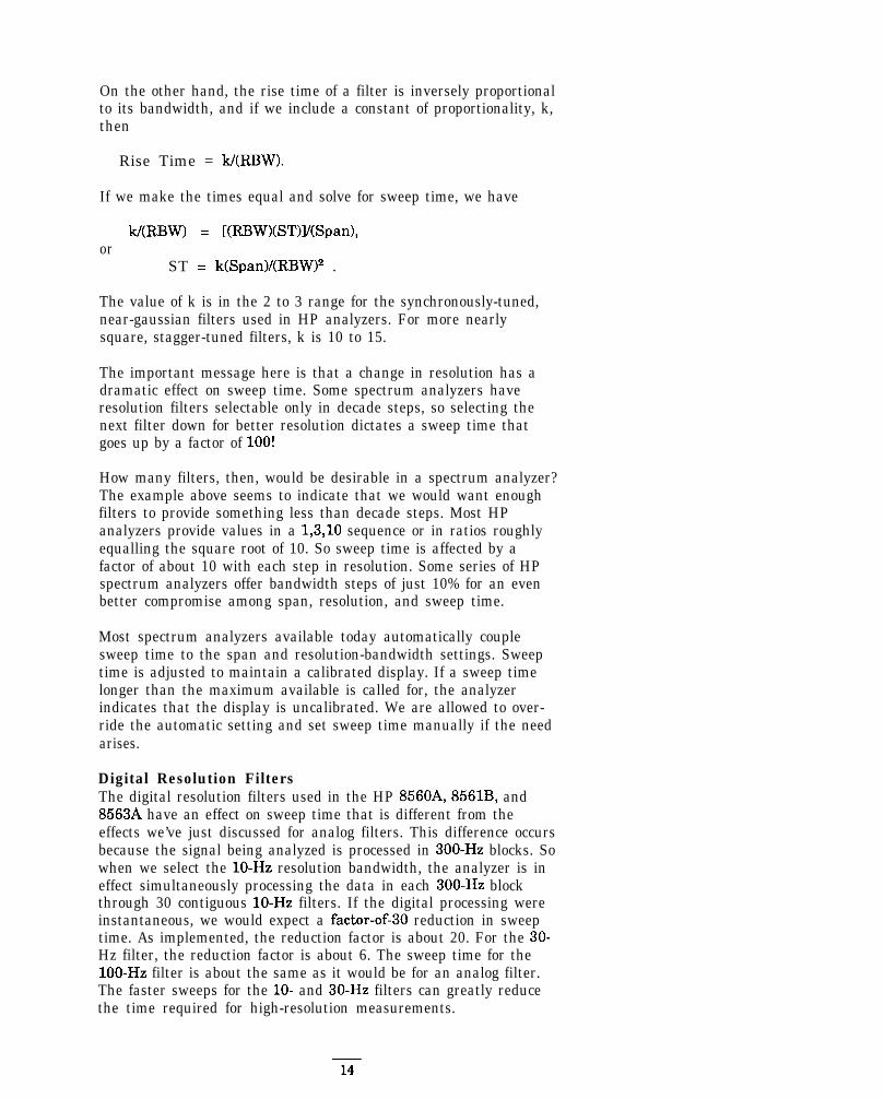
Digital Resolution FiltersThe digital resolution filters used in the HP 8560A, 8561B, and8563A have an effect on sweep time that is different from theeffects we’ve just discussed for analog filters. This difference occursbecause the signal being analyzed is processed in 300-Hz blocks. Sowhen we select the lo-Hz resolution bandwidth, the analyzer is ineffect simultaneously processing the data in each 300-Hz blockthrough 30 contiguous lo-Hz filters. If the digital processing wereinstantaneous, we would expect a factor-of-30 reduction in sweeptime. As implemented, the reduction factor is about 20. For the 30-Hz filter, the reduction factor is about 6. The sweep time for thelOO-Hz filter is about the same as it would be for an analog filter.The faster sweeps for the lo- and 30-Hz filters can greatly reducethe time required for high-resolution measurements.

Envelope DetectorSpectrum analyzers typically convert the IF signal to video’ with

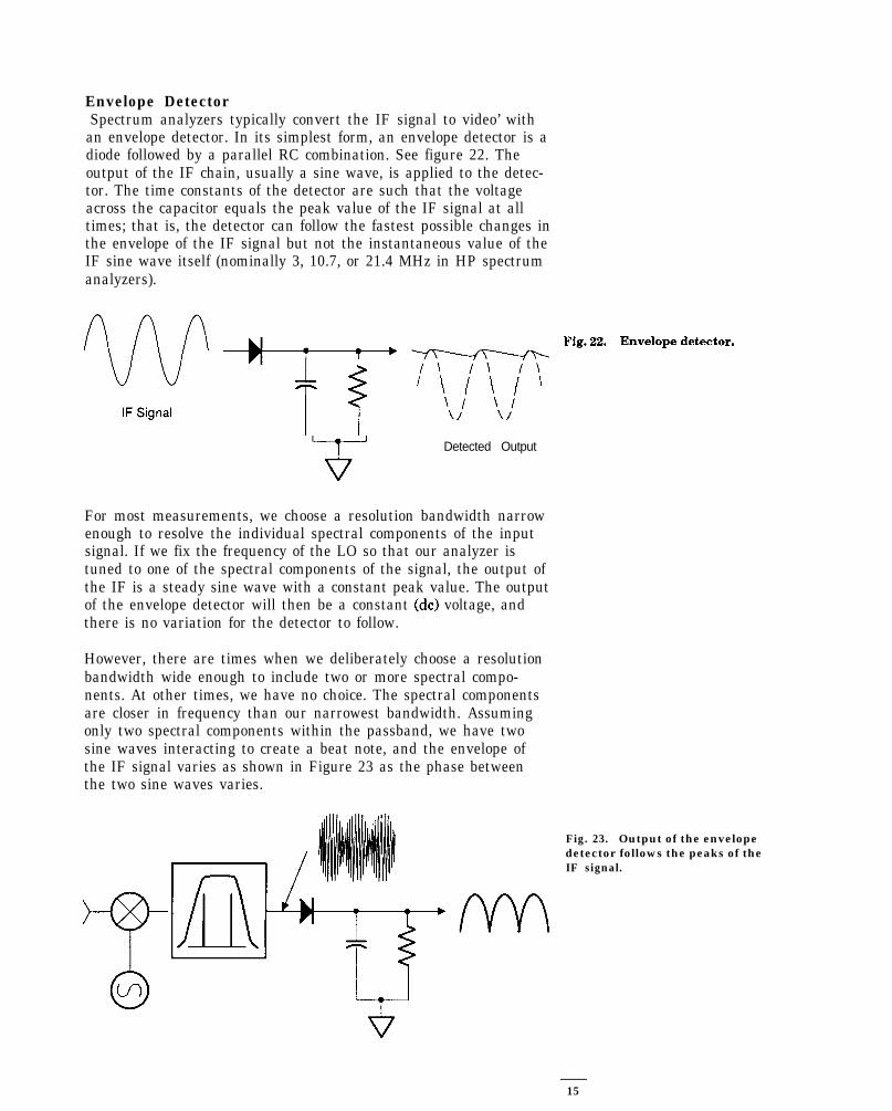
an envelope detector. In its simplest form, an envelope detector is adiode followed by a parallel RC combination. See figure 22. Theoutput of the IF chain, usually a sine wave, is applied to the detec-tor. The time constants of the detector are such that the voltageacross the capacitor equals the peak value of the IF signal at alltimes; that is, the detector can follow the fastest possible changes inthe envelope of the IF signal but not the instantaneous value of theIF sine wave itself (nominally 3, 10.7, or 21.4 MHz in HP spectrumanalyzers).

qp +-f---y qT$fy Fig.22. Envelopedetector.

Detected Output

For most measurements, we choose a resolution bandwidth narrowenough to resolve the individual spectral components of the inputsignal. If we fix the frequency of the LO so that our analyzer istuned to one of the spectral components of the signal, the output ofthe IF is a steady sine wave with a constant peak value. The outputof the envelope detector will then be a constant (dc) voltage, andthere is no variation for the detector to follow.

However, there are times when we deliberately choose a resolutionbandwidth wide enough to include two or more spectral compo-nents. At other times, we have no choice. The spectral componentsare closer in frequency than our narrowest bandwidth. Assumingonly two spectral components within the passband, we have twosine waves interacting to create a beat note, and the envelope ofthe IF signal varies as shown in Figure 23 as the phase betweenthe two sine waves varies.

Fig. 23. Output of the envelopedetector follows the peaks of theIF signal.

15

What determines the maximum rate at which the envelope of theIF signal can change? The width of the resolution (IF) filter. Thisbandwidth determines how far apart two input sinusoids can beand, after the mixing process, be within the filter at the sametime.8 If we assume a 21.4-MHz final IF and a lOO-kHz bandwidth,two input signals separated by 100 kHz would produce, with theappropriate LO frequency and two or three mixing processes,mixing products of 21.35 and 21.45 MHz and so meet the criterion.See Figure 23. The detector must be able to follow the changes inthe envelope created by these two signals but not the nominal 21.4MHz IF signal itself.

The envelope detector is what makes the spectrum analyzer avoltmeter. If we duplicate the situation above and have two equal-amplitude signals in the passband of the IF at the same time, whatwould we expect to see on the display? A power meter wouldindicate a power level 3 dB above either signal; that is, the totalpower of the two. Assuming that the two signals are close enoughso that, with the analyzer tuned half way between them, there isnegligible attenuation due to the roll-off of the filter, the analyzerdisplay will vary between a value twice the voltage of either (6 dBgreater) and zero (minus infinity on the log scale). We must re-member that the two signals are sine waves (vectors) at differentfrequencies, and so they continually change in phase with respectto each other. At some time they add exactly in phase; at another,exactly out of phase.

So the envelope detector follows the changing amplitude values ofthe peaks of the signal from the IF chain but not the instantaneousvalues. And gives the analyzer its voltmeter characteristics.

Although the digitally-implemented resolution bandwidths do nothave an analog envelope detector, one is simulated for consistency

l Fte 1.06 nllz *V!J 0.60 tlHz

with the other bandwidths. Fig. 24. Spectrum analyzers displaysignal plus noise.

Display Smoothing

Video FilteringSpectrum analyzers display signals plus their own internal noise,gas shown in Figure 24. To reduce the effect of noise on the dis-played signal amplitude, we often smooth or average the display, asshown in Figure 25. All HP superheterodyne analyzers include avariable video filter for this purpose. The video filter is a low-passfilter that follows the detector and determines the bandwidth of thevideo circuits that drive the vertical deflection system of the dis-play. As the cutoff frequency of the video filter is reduced to thepoint at which it becomes equal to or less than the bandwidth ofthe selected resolution (IF) filter, the video system can no longerfollow the more rapid variations of the envelope of the signal(s) .RS 1.18 m ST 266.7 1IBBC

passing through the IF chain. The result is an averaging orsmoothing of the displayed signal. Fig. 26. Display of Fig. 24 after full

smoothing.

16

choose permanent storage, or we could erase the display and startover. Hewlett-Packard pioneered a variable-persistence mode inwhich we could adjust the fade rate of the display. When properlyadjusted, the old trace would just fade out at the point where thenew trace was updating the display. The idea was to provide adisplay that was continuous, had no flicker, and avoided confusingoverwrites. The system worked quite well with the correct trade-offbetween trace intensity and fade rate. The difficulty was that theintensity and the fade rate had to be readjusted for each new meas-urement situation.

When digital circuitry became affordable in the mid-1970s, it wasquickly put to use in spectrum analyzers. Once a trace had beendigitized and put into memory, it was permanently available fordisplay. It became an easy matter to update the display at a flicker-free rate without blooming or fading. The data in memory wasupdated at the sweep rate, and since the contents of memory werewritten to the display at a flicker-free rate, we could follow theupdating as the analyzer swept through its selected frequency spanjust as we could with analog systems.

Digital DisplaysBut digital systems were not without problems of their own. Whatvalue should be displayed? As Figure 30 shows, no matter howmany data points we use across the CRT, each point must repre-sent what has occurred over some frequency range and, althoughwe usually do not think in terms of time when dealing with aspectrum analyzer, over some time interval. Let us imagine thesituation illustrated in Figure 30: we have a display that contains asingle CW signal and otherwise only noise. Also, we have an analogsystem whose output we wish to display as faithfully as possibleusing digital techniques.

As a first method, let us simply digitize the instantaneous value ofthe signal at the end of each interval (also called a cell or bucket).This is the sample mode. To give the trace a continuous look, wedesign a system that draws vectors between the points. From theconditions of Figure 30, it appears that we get a fairly reasonabledisplay, as shown in Figure 31. Of course, the more points in thetrace, the better the replication of the analog signal. The number ofpoints is limited, with 1,000 being the maximum typically offeredon any spectrum analyzer. As shown in Figure 32, more points doindeed get us closer to the analog signal.

While the sample mode does a good job of indicating the random-ness of noise, it is not a good mode for a spectrum analyzer’s usualfunction: analyzing sinusoids. If we were to look at a loo-MHzcomb on the HP 71210, we might set it to span from 0 to 22 GHz.Even with 1,000 display points, each point represents a span of 22GHz, far wider than the maximum ~-MHZ resolution bandwidth.

m lSrSl:36 RGG 3 , 1989

1 2 5 4 5 6 7 8 9 1 0

Fig. 30. When digitizing an analogsignal, what value should be dis-played at each point?

1 2 3 4 5 6 7 8 9 1 0

Fig. 31. The sample display modeusing ten points to display thesignal of Figure 30.

Fig. 32. More points produce adisplay closer to an analog display.

19

As a result, the true amplitude of a comb tooth is shown only if itsmixing product happens to fall at the center of the IF when thesample is taken. Figure 33 shows a 5-GHz span with a l-MHzband-width; the comb teeth should be relatively equal in amplitude.Figure 34 shows a 500-MHz span comparing the true comb with theresults from the sample mode; only a few points are used to exag-gerate the effect. (The sample trace appears shifted to the leftbecause the value is plotted at the beginning of each interval.)

One way to insure that all sinusoids are reported is to display themaximum value encountered in each cell. This is the positive-peakdisplay mode, or pos peak. This display mode is illustrated inFigure 35. Figure 36 compares pos peak and sample display modes.Pos peak is the normal or default display mode offered on manyspectrum analyzers because it ensures that no sinusoid is missed,regardless of the ratio between resolution bandwidth and cellwidth. However, unlike sample mode, pos peak does not give a goodrepresentation of random noise because it captures the crests of thenoise. So spectrum analyzers using the pos peak mode as theirprimary display mode generally also offer the sample mode as analternative.

Fig. 34. The actual comb and resultsof the sample display mode over a500-MHz span. When resolutionbandwidth is narrower than thesample interval, the sample mode cangive erroneous results. (The sampletrace has only 20 points to exagger-ate the effect.)

Fig. 33. A 6-GHx span of a lOO-MHzcomb in the sample display mode.The actual comb values are relativelyconstant over this range.

Fig. 35. Pos peak display modeversus actual comb.

Fig. 36. Comparison of sample andpos peak display modes.

To provide a better visual display of random noise than pos peakand yet avoid the missed-signal problem of the sample mode, therosenfell display mode is offered on many spectrum analyzers.Rosenfell is not a person’s name but rather a description of thealgorithm that tests to see if the signal rose and fell within the cellrepresented by a given data point. Should the signal both rise andfall, as determined by pos-peak and neg-peak detectors, then thealgorithm classifies the signal as noise. In that case, an odd-num-bered data point indicates the maximum value encountered duringits cell. On the other hand, an even-numbered data point indicatesthe minimum value encountered during its cell. Rosenfell andsample modes are compared in Figure 37.

Fig. 37. Comparison of rosenfell andsample display modes.

20

What happens when a sinusoidal signal is encountered? We knowthat as a mixing product is swept past the IF filter, an analyzertraces out the shape of the filter on the display. If the filter shape isspread over many display points, then we encounter a situation inwhich the displayed signal only rises as the mixing product ap-proaches the center frequency of the filter and only falls as themixing product moves away from the filter center frequency. Ineither of these cases, the pos-peak and neg-peak detectors sense anamplitude change in only one direction, and, according to therosenfell algorithm, the maximum value in each cell is displayed.See Figure 38.

What happens when the resolution bandwidth is narrow relative toa cell? If the peak of the response occurs anywhere but at the veryend of the cell, the signal will both rise and fall during the cell. Ifthe cell happens to be an odd-numbered one, all is well. The maxi- 1% CHz VB 338 91 10.08 w**t

mum value encountered in the cell is simply plotted as the nextdata point. However, if the cell is even-numbered, then the mini-

Fig. 38. When detected signal onlyrises or falls, as when mixing product

mum value in the cell is plotted. Depending on the ratio of resolu- sweeps past resolution filter, rosenfell

tion bandwidth to cell width, the minimum value can differ from displays maximum values.

the true peak value (the one we want displayed) by a little or a lot.In the extreme, when the cell is much wider than the resolutionbandwidth, the difference between the maximum and minimumvalues encountered in the cell is the full difference between thepeak signal value and the noise. Since the rosenfell algorithm callsfor the minimum value to be indicated during an even-numberedcell, the algorithm must include some provision for preserving themaximum value encountered in this cell.

To ensure no loss of signals, the pos-peak detector is reset onlyafter the peak value has been used on the display. Otherwise, thepeak value is carried over to the next cell. Thus when a signal bothrises and falls in an even-numbered cell, and the minimum value isdisplayed, the pos-peak detector is not reset. The pos-peak value iscarried over to the next cell, an odd-numbered cell. During this cell,the pos-peak value is updated only if the signal value exceeds thevalue carried over. The displayed value, then, is the larger of theheld-over value and the maximum value encountered in the new,odd-numbered cell. Only then is the pos-peak detector reset.

This process may cause a maximum value to be displayed one datapoint too far to the right, but the offset is usually only a smallpercentage of the span. Figure 39 shows what might happen insuch a case. A small number of data points exaggerates the effect.

The rosenfell display mode does a better job of combining noise anddiscrete spectral components on the display than does pos peak. Weget a much better feeling for the noise with rosenfell. However,

Fig. 39. Rosenfell when signal peakfalls between data points (fewer trace

because it allows only maxima and minima to be displayed, rosen-fell does not give us the true randomness of noise as the samplemode does. For noise signals, then, the sample display mode is thebest.

pointa exaggerate the effect).

21

HP analyzers that use rosenfell as their default, or normal, displaymode also allow selection of the other display modes - pos peak, negpeak, and sample.

As we have seen, digital displays distort signals in the process ofgetting them to the screen. However, the pluses of digital displaysgreatly outweigh the minuses. Not only can the digital informationbe stored indefinitely and refreshed on the screen without flicker,blooming, or fade, but once data is in memory, we can add capabili-ties such as markers and display arithmetic or output data to acomputer for analysis or further digital signal processing.

Amplitude Accuracy

Now that we have our signal displayed on the CRT, let’s look atamplitude accuracy. Or, perhaps better, amplitude uncertainty.Most spectrum analyzers these days are specified in terms of bothabsolute and relative accuracy. However, relative performanceaffects both, so let us look at those factors affecting relative meas-urement uncertainty first.

Relative UncertaintyWhen we make relative measurements on an incoming signal, weuse some part of the signal as a reference. For example, when wemake second-harmonic distortion measurements, we use the funda-mental of the signal as our reference. Absolute values do not comeinto play;12 we are interested only in how the second harmonicdiffers in amplitude from the fundamental.

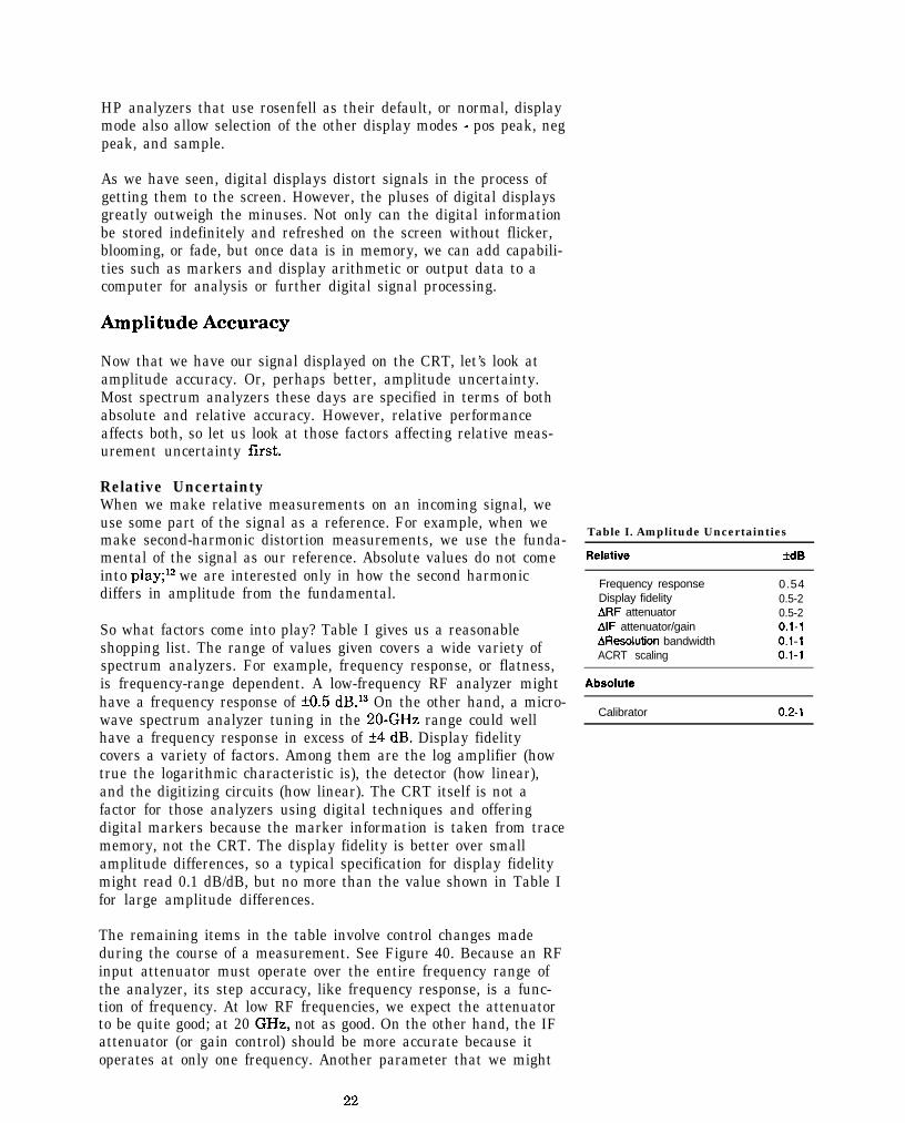
So what factors come into play? Table I gives us a reasonableshopping list. The range of values given covers a wide variety ofspectrum analyzers. For example, frequency response, or flatness,is frequency-range dependent. A low-frequency RF analyzer mighthave a frequency response of +0.5 dB.13 On the other hand, a micro-wave spectrum analyzer tuning in the 20-GHz range could wellhave a frequency response in excess of ?4 dB. Display fidelitycovers a variety of factors. Among them are the log amplifier (howtrue the logarithmic characteristic is), the detector (how linear),and the digitizing circuits (how linear). The CRT itself is not afactor for those analyzers using digital techniques and offeringdigital markers because the marker information is taken from tracememory, not the CRT. The display fidelity is better over smallamplitude differences, so a typical specification for display fidelitymight read 0.1 dB/dB, but no more than the value shown in Table Ifor large amplitude differences.

The remaining items in the table involve control changes madeduring the course of a measurement. See Figure 40. Because an RFinput attenuator must operate over the entire frequency range ofthe analyzer, its step accuracy, like frequency response, is a func-tion of frequency. At low RF frequencies, we expect the attenuatorto be quite good; at 20 GHz, not as good. On the other hand, the IFattenuator (or gain control) should be more accurate because itoperates at only one frequency. Another parameter that we might

Table I. Amplitude Uncertainties

Relative MB

Frequency response 0.54Display fidelity 0.5-2ARF attenuator 0.5-2AIF attenuator/gain 0.1-lAResolution bandwidth 0.1-lACRT scaling 0.1-l

Absolute

Calibrator 0.2-l

22

change during the course of a measurement is resolution band-width. Different filters have different insertion losses. Generally wesee the greatest difference when switching between inductor-capacitor (LC) filters, typically used for the wider resolution band-widths, and crystal filters. Finally, we may wish to change displayscaling from, say, 10 dB/div to 1 dB/div or linear.

A factor in measurement uncertainty not covered in the table isimpedance mismatch. Analyzers do not have perfect input imped-ances, nor do most signal sources have ideal output impedances.However, in most cases uncertainty due to mismatch is relativelysmall. Improving the match of either the source or analyzer reducesuncertainty. Since an analyzer’s match is worst with its inputattenuator set to 0 dB, we should avoid the 0-dB setting if we can. Ifneed be, we can attach a well-matched pad (attenuator) to theanalyzer input and so effectively remove mismatch as a factor.

3c/ Fig. 40. Controls that affectr>L/ amplitude accuracy.rL

1IR.F. IF RES

ATTEN Anen/Gain SW

Absolute AccuracyThe last item in Table I is the calibrator, which gives the spectrumanalyzer its absolute calibration. For convenience, calibrators aretypically built into today’s spectrum analyzers and provide a signalwith a specified amplitude at a given frequency. We then rely onthe relative accuracy of the analyzer to translate the absolute cali-bration to other frequencies and amplitudes.

Improving Overall UncertaintyIf we are looking at measurement uncertainty for the first time, wemay well be concerned as we mentally add up the uncertaintyfigures. And even though we tell ourselves that these are worst-case values and that almost never are all factors at their worst andin the same direction at the same time, still we must add thefigures directly if we are to certify the accuracy of a specific meas-urement.

There are some things that we can do to improve the situation.First of all, we should know the specifications for our particularspectrum analyzer. These specifications may be good enough overthe range in which we are making our measurement. If not, Table Isuggests some opportunities to improve accuracy.

Before taking any data, we can step through a measurement to seeif any controls can be left unchanged. We might find that a givenRF attenuator setting, a given resolution bandwidth, and a givendisplay scaling suffice for the measurement. If so, all uncertaintiesassociated with changing these controls drop out. We may be able to

23

trade off IF attenuation against display fidelity, using whichever ismore accurate and eliminating the other as an uncertainty factor.We can even get around frequency response if we are willing to goto the trouble of characterizing our particular analyzer.14 The sameapplies to the calibrator. If we have a more accurate calibrator, orone closer to the frequency of interest, we may wish to use that inlieu of the built-in calibrator.

Finally, many analyzers available today have self-calibrationroutines. These routines generate error coefficients (for example,amplitude changes versus resolution bandwidth) that the analyzeruses later to correct measured data. The smaller values shown inTable I, 0.5 dB for display fidelity and 0.1 dB for changes in IF at-tenuation, resolution bandwidth, and display scaling, are based oncorrected data. As a result, these self-calibration routines allow usto make good amplitude measurements with a spectrum analyzerand give us more freedom to change controls during the course of ameasurement.

SensitivityOne of the primary uses of a spectrum analyzer is to search out andmeasure low-level signals. The ultimate limitation in these meas-urements is the random noise generated by the spectrum analyzeritself. This noise, generated by the random electron motionthroughout the various circuit elements, is amplified by the variousgain stages in the analyzer and ultimately appears on the displayas a noise signal below which we cannot make measurements. Alikely starting point for noise seen on the display is the first stageof gain in the analyzer. This amplifier boosts the noise generatedby its input termination plus adds some of its own. As the noisesignal passes on through the system, it is typically high enough inamplitude that the noise generated in subsequent gain stages addsonly a small amount to the noise power. It is true that the input at-tenuator and one or more mixers may be between the input connec-tor of a spectrum analyzer and the first stage of gain, and all ofthese components generate noise. However, the noise that theygenerate is at or near the absolute minimum of -174 dBm/Hz (LTB),the same as at the input termination of the first gain stage, so theydo not significantly affect the noise level input to, and amplified by,the first gain stage.

While the input attenuator, mixer, and other circuit elementsbetween the input connector and first gain stage have little effecton the actual system noise, they do have a marked effect on theability of an analyzer to display low-level signals because theyattenuate the input signal. That is, they reduce the signal-to-noiseratio and so degrade sensitivity.

We can determine sensitivity simply by noting the noise levelindicated on the display with no input signal applied. This level isthe analyzer’s own noise floor. Signals below this level are maskedby the noise and cannot be seen or measured. However, the dis-played noise floor is not the actual noise level at the input butrather the effective noise level. An analyzer display is calibrated to

24

reflect the level of a signal at the analyzer input, so the displayednoise floor represents a fictitious (we have called it an effective)noise floor at the input below which we cannot make measure-ments. The actual noise level at the input is a function of the inputsignal. Indeed, noise is sometimes the signal of interest. Like anydiscrete signal, a noise signal must be above the effective (dis-played) noise floor to be measured. The effective input noise floorincludes the losses (attenuation) of the input attenuator, mixer(s),etc., prior to the first gain stage.

We cannot do anything about the conversion loss of the mixers, butwe do have control over the RF input attenuator. By changing thevalue of input attenuation, we change the attenuation of the inputsignal and so change the displayed signal-to-noise-floor ratio, thelevel of the effective noise floor at the input of the analyzer, and thesensitivity. We get the best sensitivity by selecting minimum (zero)RF attenuation.

Different analyzers handle the change of input attenuation indifferent ways. Because the input attenuator has no effect on theactual noise generated in the system, some analyzers simply leavethe displayed noise at the same position on the display regardless ofthe input-attenuator setting. That is, the IF gain remains constant.This being the case, the input attenuator will affect the location ofa true input signal on the display. As we increase input attenu-ation, further attenuating the input signal, the location of thesignal on the display goes down while the noise remains stationary.To maintain absolute calibration so that the actual input signalalways has the same reading, the analyzer changes the indicatedreference level (the value of the top line of the graticule). Thisdesign is used in older HP analyzers.

In newer HP analyzers, starting with the HP 85688, an internalmicroprocessor changes the IF gain to offset changes in the inputattenuator. Thus, true input signals remain stationary on thedisplay as we change the input attenuator, while the displayednoise moves up and down. In this case, the reference level remainsunchanged. See Figures 41 and 42. In either case, we get the bestsignal-to-noise ratio (sensitivity) by selecting minimum inputattenuation.

Resolution bandwidth also affects signal-to-noise ratio, or sensitiv-ity. The noise generated in the analyzer is random and has aconstant amplitude over a wide frequency range. Since the resolu-tion, or IF, bandwidth filters come after the first gain stage, thetotal noise power that passes through the filters is determined bythe width of the filters. This noise signal is detected and ultimatelyreaches the display. The random nature of the noise signal causesthe displayed level to vary as

lO*log(bw.jbw,),where bw 1 = starting resolution bandwidth and

bw 2 = ending resolution bandwidth.

Fig. 41. Some spectrum analyzerschange reference level when RFattenuator is changed, so an inputsignal moves on the display, but theanalyzeis noise does not.

Fig. 42. Other analyzers keepreference level constant by changingIF gain, so as RF attenuator ischanged, the analyzer’s noise moves,but an input signal does not.

25

So if we change the resolution bandwidth by a factor of 10, thedisplayed noise level changes by 10 dBi5, as shown in Figure 43.We get best signal-to-noise ratio, or best sensitivity, using the mini-mum resolution bandwidth available in our spectrum analyzer.

A spectrum analyzer displays signal plus noise, and a low signal-to-noise ratio makes the signal difficult to distinguish. We notedabove that the video filter can be used to reduce the amplitude fluc-tuations of noisy signals while at the same time having no effect onconstant signals. Figure 44 shows how the video filter can improveour ability to discern low-level signals. It should be noted that thevideo filter does not affect the average noise level and so does not,strictly speaking, affect the sensitivity of an analyzer.

In summary, we get best sensitivity by selecting the minimumresolution bandwidth and minimum input attenuation. Thesesettings give us best signal-to-noise ratio. We can also select mini-mum video bandwidth to help us see a signal at or close to thenoise level.16 Of course, selecting narrow resolution and video band-widths does lengthen the sweep time.

Noise FigureMany receiver manufacturers specify the performance of theirreceivers in terms of noise figure rather than sensitivity. As weshall see, the two can be equated. A spectrum analyzer is a re-ceiver, and we shall examine noise figure on the basis of a sinu-soidal input.

IR 9.s *.*

Fig. 43. Displayed noise level changesas lO*log(BW,/BW,).

Noise figure can be defined as the degradation of signal-to-noiseratio as a signal passes through a device, a spectrum analyzer inour case. We can express noise figure as

F = (S,/N,Y(So/N,,),where F = noise figure as power ratio,

Si = input signal power,Ni = true input noise power,so = output signal power, andNo = output noise power.

If we examine this expression, we can simplify it for our spectrumanalyzer. First of all, the output signal is the input signal times the

Fig. 44. Video filtering makes low-1eve1 signals more discernable. (The

gain of the analyzer. Second, the gain of our analyzer is unity average trace was offset for visibility.)

because the signal level at the output (indicated on the display) isthe same as the level at the input (input connector). So our expres-sion, after substitution, cancellation, and rearrangement, becomes

F = No/N,.

This expression tells us that all we need to do to determine thenoise figure is compare the noise level as read on the display to thetrue (not the effective) noise level at the input connector. Noisefigure is usually expressed in terms of dB, or

NF = lO*log(F) = 10*log(NO) - lO*log(N,).

26

We use the true noise level at the input rather than the effectivenoise level because our input signal-to-noise ratio was based on thetrue noise. Now we can obtain the true noise at the input simply byterminating the input in 50 ohms. The input noise level thenbecomes

N, = kTB,

where k = Boltzmann’s constant,T = absolute temperature in degrees kelvin, andB = bandwidth.

At room temperature and for a l-Hz bandwidth,

kTB = -174 dBm.

We know that the displayed level of noise on the analyzer changeswith bandwidth. So all we need to do to determine the noise figureof our spectrum analyzer is to measure the noise power in somebandwidth, calculate the noise power that we would have measuredin a l-Hz bandwidth using lO*log(bwJbw,), and compare that to-174 dBm. For example, if we measured -110 dBm in a lo-kHzresolution bandwidth, we would get

NF = (measured noise),m,, - lO*log(RBW/l) - kTB,_,

= -110 dBm - 10*1og(10,000/1) - (-174 dBm)= -110 - 40 + 174= 24 dB.

Noise figure is independent of bandwidth17. Had we selected adifferent resolution bandwidth, our results would have been exactlythe same. For example, had we chosen a l-kHz resolution band-width, the measured noise would have been -120 dBm andlO*log(RBW/l) would have been 30. Combining all terms wouldhave given -120 - 30 + 174 = 24 dB, the same noise figure as above.

The 24-dB noise figure in our example tells us that a sinusoidalsignal must be 24 dB above kTB to be equal to the average dis-played noise on this particular analyzer. Thus we can use noisefigure to determine sensitivity for a given bandwidth or to comparesensitivities of different analyzers on the same bandwidth.18

PreamplifiersOne reason for introducing noise figure is that it helps us deter-mine how much benefit we can derive from the use of a preampli-fier. A 24-dB noise figure, while good for a spectrum analyzer, isnot so good for a dedicated receiver. However, by placing an appro-priate preamplifier in front of the spectrum analyzer, we can obtaina system (preamplifier/spectrum analyzer) noise figure that islower than that of the spectrum analyzer alone. To the extent thatwe lower the noise figure, we also improve the system sensitivity.

27

the preamplifier less 2.5 dB, or 5.5 dB. In a lo-kHz resolution band-width our preamplifier/analyzer system has a sensitivity of

kTB,_, + lO*log(RBW/ll + NF,,,

= -174 dBm + 40 dB + 5.5 dB= -128.5 dBm.

This is an improvement of 18.5 dB over the -110 dBm noise floorwithout the preamplifier.

Is there any drawback to using this preamplifier? That dependsupon our ultimate measurement objective. If we want the bestsensitivity but no loss of measurement range, then this preampli-tier is not the right choice. Figure 45 illustrates this point. Aspectrum analyzer with a 24-dB noise figure will have an averagedisplayed noise level of -110 dBm in a lo-kHz resolution band-width. If the l-dB compression pointlg for that analyzer is -10 dBm,the measurement range is 100 dB. When we connect the preamp-lifier, we must reduce the maximum input to the system by thegain of the pre-amplifier to -46 dBm. However, when we connectthe preamplifier, the noise as displayed on the CRT will rise byabout 17.5 dB because the noise power out of the preamplifier isthat much higher than the analyzer’s own noise floor, even after ac-counting for the 2.5-dB factor. It is from this higher noise level thatwe now subtract the gain of the preamplifier. With the preamplifierin place, our measurement range is 82.5 dB, 17.5 dB less thanwithout the preamplifier. The loss in measurement range equalsthe change in the displayed noise when the preamplifier is con-nected.

SpectrumAnalyzer

-10 dBm-t dS csmprassion

1OOdBSpa&urnAnalyzer

Range

1

Avg. noteson CRT

-110 d&n/l0 kHz

Spectrum Analyzer& Preamplifier

--------

}QPm

82.5 dSSystemRange

System 1 dS-46 dSm

cDmprsssion

Avg. noiseon CRT

Systemsensitivity

Is there a preamplifier that will give us better sensitivity withoutcosting us measurement range? Yes. But it must meet the second ofthe above criteria; that is, the sum of its gain and noise figure mustbe at least 10 dB less than the noise figure of the spectrum ana-lyzer. In this case the displayed noise floor will not change notice-ably when we connect the preamplifier, so although we shift thewhole measurement range down by the gain of the preamplifier, weend up with the same overall range that we started with.

Fig. 45. If the displayed noise goesup when a preamplifier is connected,measurement range is diminished bythe amount the noise changes.

29

If we use 10*log(bwz/bw,l to adjust the displayed noise level to whatwe would have measured in a noise power bandwidth of the samenumeric value as our 3-dB bandwidth, we find that the adjustmentvaries from

10*1og(10,000/10,500) = -0.21 dB to10*1og(10,000/11,300) = -0.53 dB.

In other words, if we subtract something between 0.21 and 0.53 dBfrom the indicated noise level, we shall have the noise level in anoise-power bandwidth that is convenient for computations.

Let’s consider all three factors and calculate a total correction:

Rayleigh distribution (linear mode): 1.05 dBlog amplifier (log mode): 1.45 dB

3-dB/noise power bandwidths: -0.5 dB- - - - - - - -

total correction: 2.0 dB

Here we use -0.5 dB as a reasonable compromise for the bandwidthcorrection. The total correction is thus a convenient value.

Many of today’s microprocessor-controlled analyzers allow us toactivate a noise marker. When we do so, the microprocessorswitches the analyzer into the sample display mode, computes themean value of the 32 display points about the marker, adds theabove 2-dB amplitude correction, normalizes the value to a l-Hznoise-power bandwidth, and displays the normalized value.

The analyzer does the hard part. It is reasonably easy to convertthe noise-marker value to other bandwidths. For example, if wewant to know the total noise in a ~-MHZ communication channel,we add 66 dB to the noise-marker value (60 dB for the 1,000,000/1and another 6 dB for the additional factor of four).

Preamplifier for Noise MeasurementsSince noise signals are typically low-level signals, we often need apreamplifier to have sufficient sensitivity to measure them. How-ever, we must recalculate sensitivity of our analyzer first. Above,we defined sensitivity as the level of a sinusoidal signal that isequal to the displayed average noise floor. Since the analyzer iscalibrated to show the proper amplitude of a sinusoid, no correctionfor the signal was needed. But noise is displayed 2.5 dB too low, soan input noise signal must be 2.5 dB above the analyzer’s displayednoise floor to be at the same level by the time it reaches the display.The input and internal noise signals add to raise the displayednoise by 3 dB, a factor of two in power. So we can define the noisefigure of our analyzer for a noise signal as

NFB,,, = (noise floor)dBmm, - lO*log(RBW/l) - kTB,_, + 2.5 dB.

33

If we use the same noise floor as above, -110 dBm in a lo-kHzresolution bandwidth, we get

NF,, = -110 dBm - 10*1og(10,000/1)- (174 dBm)+2.5 dB = 26.5 dB.

As was the case for a sinusoidal signal, NF,,, is independent ofresolution bandwidth and tells us how far above kTB a noise signalmust be to be equal to the noise floor of our analyzer.

When we add a preamplifier to our analyzer, the system noisefigure and sensitivity improve. However, we have accounted for the2.5-dB factor in our definition of NF,,, so the graph of systemnoise figure becomes that of Figure 49. We determine system noisefigure for noise the same way that we did for a sinusoidal signalabove.

System NoiseFigureWI

NFwNjGp+ 3 dB

NFw, jGpre+ 2 dB

NFw,,).Gm+ 1 dB

NFSA(NjGpe-10 -5 0 +5

NFp. + Gpe-NFwNj NW

+lO

NFpm + 3 dB

NFp, + 2 dB

NFp,e + 1 d8

NFpe

Dynamic Range

DefinitionDynamic range is generally thought of as the ability of an analyzerto measure harmonically related signals and the interaction of twoor more signals; for example, to measure second- or third-harmonicdistortion or third-order intermodulation. In dealing with suchmeasurements, remember that the input mixer of a spectrumanalyzer is a non-linear device and so always generates distortionof its own. The mixer is non-linear for a reason. It must be non-linear to translate an input signal to the desired IF. But the un-wanted distortion products generated in the mixer fall at the samefrequencies as do the distortion products we wish to measure on theinput signal.

So we might define dynamic range in this way: it is the ratio,expressed in dB, of the largest to the smallest signals simul-taneously present at the input of the spectrum analyzer that allowsmeasurement of the smaller signal to a given degree of uncertainty.

Fig. 49. System noise figure forsignals.

Notice that accuracy of the measurement is part of the definition.We shall see how both internally generated noise and distortionaffect accuracy below.

34

Dynamic Range versus Internal DistortionTo determine dynamic range versus distortion, we must first deter-mine just how our input mixer behaves. Most analyzers, particu-larly those utilizing harmonic mixing to extend their tuning range,21use diode mixers. (Other types of mixers would behave similarly.)The current through an ideal diode can be expressed as

i = IS(evkT - 11,

where q = electronic charge,v = instantaneous voltage,k = Boltzmann’s constant, andT = temperature in degrees Kelvin.

We can expand this expression into a power series

i = J(k,v + k2v2 + k3v3 + . ..).

where k, = q/kTk, = ki2/2!,k, = ki3/3!, etc.

Let’s now apply two signals to the mixer. One will be the inputsignal that we wish to analyze; the other, the local oscillator signalnecessary to create the IF:

v = V,,sin(w,,t) + V,sin(w,t).

If we go through the mathematics, we arrive at the desired mixingproduct that, with the correct LO frequency, equals the IF:

k2VLoV,cd(w,, - wiltI.

A k,V,oV,cos[(w,, + wilt1 term is also generated, but in our dis-cussion of the tuning equation, we found that we want the LO to beabove the IF, so (wLo + wi) is also always above the IF.

With a constant LO level, the mixer output is linearly related to theinput signal level. For all practical purposes, this is true as long asthe input signal is more than 15 to 20 dB below the level of the LO.There are also terms involving harmonics of the input signal:

(3k~4lV,oV,2sin(w,, - 2w,)t,(k,/8)V,,V,3sin(w,o - 3w,)t, etc.

These terms tell us that dynamic range due to internal distortion isa function of the input signal level at the input mixer. Let’s see howthis works, using as our definition of dynamic range the differencein dB between the fundamental tone and the internally generateddistortion.

35

The argument of the sine in the first term includes 2w1, so it repre-sents the second harmonic of the input signal. The level of thissecond harmonic is a function of the square of the voltage of thefundamental, Vi2. This fact tells us that for every dB that we dropthe level of the fundamental at the input mixer, the internallygenerated second harmonic drops by 2 dB. See Figure 50. Thesecond term includes 3wl, the third harmonic, and the cube of theinput-signal voltage, V,3. So a l-dB change in the fundamental atthe input mixer changes the internally generated third harmonicby 3 dB.

2AdB3AdB

3AdB

AdB I

i

hdB

W 2w 3W 2w1-w2 Wl w2 2w2-w 1

Distortion is often described by its order. The order can be deter-mined by noting the coefficient associated with the signal frequencyor the exponent associated with the signal amplitude. Thus second-harmonic distortion is second order and third harmonic distortionis third order. The order also indicates the change in internallygenerated distortion relative to the change in the fundamental tonethat created it.

Now let us add a second input signal:

v = V,,sin(w,ot) + V,sin(w,t) + V,sin(w,t).

This time when we go through the math to find internally gener-ated distortion, in addition to harmonic distortion, we get

(k(8WLoV,2V2cos[w,o - (2w, - w,llt,

(k,/8)VLoV,V22cos[w,o - (2w, - w,)lt, etc.

These represent intermodulation distortion, the interaction of thetwo input signals with each other. The lower distortion product,2w, - w2, falls below wr by a frequency equal to the differencebetween the two fundamental tones, w2 - wi. The higher distortionproduct, 2w, - wr, falls above wp by the same frequency.See Figure 50.

Fig. 50. Changing the level offundamental tone (w) or tones (w,,WJ at the mixer affects internallygenerated distortion.

3AdB

Once again, dynamic range is a function of the level at the inputmixer. The internally generated distortion changes as the productof V,2 and V, in the first case, of V, and V22 in the second. If V, andV, have the same amplitude, the usual case when testing for distor-

36

tion, we can treat their products as cubed terms (VI3 or VZ3). Thus,for every dB that we simultaneously change the level of the twoinput signals, there is a 3-dB change in the distortion componentsas shown in Figure 50.

This is the same degree of change that we saw for third harmonicdistortion above. And in fact, this, too, is third-order distortion. Inthis case, we can determine the degree of distortion by summing thecoefficients of w1 and w2 or the exponents of V, and V,.

All this says that dynamic range depends upon the signal level atthe mixer. How do we know what level we need at the mixer for aparticular measurement? Many analyzer data sheets now includegraphs to tell us how dynamic range varies. However, if no graph isprovided, we can draw our own.

We do need a starting point, and this we must get from the datasheet. We shall look at second-order distortion first. Let’s assumethe data sheet says that second-harmonic distortion is 70 dB downfor a signal -40 dBm at the mixer. Because distortion is a relativemeasurement, and, at least for the moment, we are calling ourdynamic range the difference in dB between fundamental tone ortones and the internally generated distortion, we have our startingpoint. Internally generated second-order distortion is 70 dB down,so we can measure distortion down 70 dB. We plot that point on agraph whose axes are labeled distortion (dBc) versus level at themixer (level at the input connector minus the input-attenuatorsetting). See Figure 51. What happens if the level at the mixerdrops to -50 dBm? As noted above (Figure 501, for every dB changein the level of the fundamental at the mixer there is a 2-dB changein the internally generated second harmonic. But for measurementpurposes, we are only interested in the relative change, that is, inwhat happened to our measurement range. In this case, for everydB that the fundamental changes at the mixer, our measurementrange aIso changes by 1 dB. In our second-harmonic example, then,when the level at the mixer changes from -40 to -50 dBm, theinternal distortion, and thus our measurement range, changes from-70 to -80 dBc. In fact, these points fall on a line with a slope of 1that describes the dynamic range for any input level at the mixer.

We can construct a similar line for third-order distortion. Forexample, a data sheet might say third-order distortion is -70 dBc fora level of -30 dBm at this mixer. Again, this is our starting point,and we would plot the point shown in Figure 51. If we now drop thelevel at the mixer to -40 dBm, what happens? Referring again toFigure 50, we see that both third-harmonic distortion and third-order inter-modulation distortion fall by 3 dB for every dB that thefundamental tone or tones fall. Again it is the difference that isimportant. If the level at the mixer changes from -30 to -40 dBm,the difference between fundamental tone or tones and internallygenerated distortion changes by 20 dB. So the internal distortion is-90 dBc. These two points fall on a line having a slope of 2, giving usthe third-order performance for any level at the mixer.

Ol-10

s

8

TOI

I

-60 -50 4 0 -30 -20 -10 0 +lO

Mixer Level (dBm)

Fig. 51. Dynamic range versusdistortion and noise.

37

of -40 dBm at the mixer, it is 70 dB above the average noise, so wehave 70 dB signal-to-noise ratio. For every dB that we reduce thesignal level at the mixer, we lose 1 dB of signal-to-noise ratio. Ournoise curve is a straight line having a slope of -1, as shown inFigure 51.

Under what conditions, then, do we get the best dynamic range?Without regard to measurement accuracy, it would be at the inter-section of the appropriate distortion curve and the noise curve.Figure 51 tells us that our maximum dynamic range for second-order distortion is 70 dB; for third-order distortion, 77 dB.

Figure 51 shows the dynamic range for one resolution bandwidth.We certainly can improve dynamic range by narrowing the resolu-tion bandwidth, but there is not a one-to-one correspondencebetween the lowered noise floor and the improvement in dynamicrange. For second-order distortion the improvement is one half thechange in the noise floor; for third-order distortion, two thirds thechange in the noise floor. See Figure 52.

The final factor in dynamic range is the phase noise on our spec-trum analyzer LO, and this affects only third-order distortionmeasurements. For example, suppose we are making a two-tone,third-order distortion measurement on an amplifier, and our testtones are separated by 10 kHz. The third-order distortion com-ponents will be separated from the test tones by 10 kHz also. Forthis measurement we might find ourselves using a 1-kHz resolutionbandwidth. Referring to Figure 52 and allowing for a lo-dB de-crease in the noise curve, we would find a maximum dynamicrange of about 84 dB. However, what happens if our phase noise ata lo-kHz offset is only -75 dBc? Then 75 dB becomes the ultimatelimit of dynamic range for this measurement, as shown in Fig. 53.

In summary, the dynamic range of a spectrum analyzer is limitedby three factors: the distortion performance of the input mixer, thebroadband noise floor (sensitivity) of the system, and the phasenoise of the local oscillator.

Dynamic Range versus Measurement UncertaintyIn our previous discussion of amplitude accuracy, we included onlythose items listed in Table I plus mismatch. We did not cover thepossibility of an internally generated distortion product (a sinusoid)being at the same frequency as an external signal that we wishedto measure. However, internally generated distortion componentsfall at exactly the same frequencies as the distortion componentswe wish to measure on external signals. The problem is that wehave no way of knowing the phase relationship between the exter-nal and internal signals. So we can only determine a potentialrange of uncertainty:

Uncertainty (in dB) = 2O*log(l+ 10dno),

where d = difference in dB between larger and smallersinusoid (a negative number).

Ol-10

I. Noise

/ \ (10 kHz BW)

,-508P

-60

-70

-80

-90

60 -50 -40 30 -20 -10 0 +lO

Mxer Level (dBm)

Fig. 52. Reducing resolutionbandwidth improves dynamic range.

/3 rdO&Jr

1

-60 -50 4 0 -30 -20 -10 0 +lO

Mixer Level (dBm)

Fig. 53. Phase noise can limit third-order intermodulation tests.

39

See Figure 54. For example, if we set up conditions such that theinternally generated distortion is equal in amplitude to the distor-tion on the incoming signal, the error in the measurement couldrange from +6 dB (the two signals exactly in phase) to -infinity (thetwo signals exactly out of phase and so cancelling). Such uncer-tainty is unacceptable in most cases. If we put a limit of 1 dB on themeasurement uncertainty, Figure 54 shows us that the internallygenerated distortion product must be about 18 dB below the distor-tion product that we wish to measure. To draw dynamic-rangecurves for second- and third-order measurements with no morethan 1 dB of measurement error, we must then offset the curves ofFigure 51 by 18 dB as shown in Figure 55.

Next let’s look at uncertainty due to low signal-to-noise ratio. Thedistortion components we wish to measure are, we hope, low-levelsignals, and often they are at or very close to the noise level of ourspectrum analyzer. In such cases we often use the video filter tomake these low-level signals more discernable. Figure 56 shows theerror in displayed signal level as a function of displayed signal-to-noise for a typical spectrum analyzer. Note that the error is only inone direction, so we could correct for it. However, we usually donot. So for our dynamic-range measurement, let’s accept a 0.5-dBerror due to noise and offset the noise curve in our dynamic-rangechart by 5 dB as shown in Figure 55. Where the distortion andnoise curves intersect, the maximum error possible would be lessthan 1.5 dB.

Let’s see what happened to our dynamic range as a result of ourconcern with measurement error. As Figure 55 shows, second-order-distortion dynamic range changes from 70 to 56.5 dB, achange of 11.5 dB. This is one half the total offsets for the twocurves (18 dB for distortion; 5 dB for noise). Third-order distortionchanges from 77 dB to about 68 dB for a change of about 9 dB. Inthis case the change is one third of the 1%dB offset for the distor-tion curve plus two thirds of the 5-dB offset for the noise curve.

Mixer CompressionIn our discussion of dynamic range, we did not concern ourselveswith how accurately the larger tone is displayed, even on a relativebasis. As we raise the level of a sinusoidal input signal, eventuallythe level at the input mixer becomes so high that the desiredoutput mixing product no longer changes linearly with respect tothe input signal. The mixer is in saturation, and the displayedsignal amplitude is too low.

Saturation is gradual rather than sudden. To help us stay awayfrom the saturation condition, the 0.5-dB or 1-dB compression pointis usually specified. A mixer level of -10 to -5 dBm is typical. Thuswe can determine what input attenuator setting to use for accuratemeasurement of high-level signals.22

Max

Error

W

Fig. 54. Uncertainty versus differencein amplitude between two sinusoids atthe same frequency.

B

Q

40 -50 -40 -30 -20 -10 0 +I0

Mixer Level (dBm)

Fig. 56. Dynamic range for 1.5-dBmaximum error.

-6.0 dB

4.0 d0

-2.0 d!3

02.0 dB 4OdB 6.0 d0 9.0 dB

Oiqlplayed 6/N (de)

Fig. 56. Error in displayed signalamplitude due to noise.

40

Actually, there are three different methods of evaluating com-pression. The traditional method, called CW compression, measuresthe change in gain of a device (amplifier or mixer or system) as theinput signal power is swept upward. This method is the one justdescribed. Note that the CW compression point is considerablyhigher than the levels for the fundamentals indicated above foreven moderate dynamic range. So we were correct in not concern-ing ourselves with the possibility of compression of the largersignal(s).

A second method, called two-tone compression, measures thechange in system gain for a small signal while the power of a largersignal is swept upward. Two-tone compression applies to themeasurement of multiple CW signals, such as sidebands and inde-pendent signals. The threshold of compression of this method isusually a few dB lower than that of the CW method.

A final method, called pulse compression, measures the change insystem gain to a narrow (broadband) RF pulse while the power ofthe pulse is swept upward. When measuring pulses, we often use aresolution bandwidth much narrower than the bandwidth of thepulse, so our analyzer displays the signal level well below the peakpulse power.= As a result, we could be unaware of the fact that thetotal signal power is above the mixer compression threshold. A highthreshold improves signal-to-noise ratio for high-power, ultra-narrow or widely chirped pulses. The threshold is about 12 dBhigher than for two-tone compression in the HP 856OA, 8561A/B,and 8562ALEVC analyzers. Nevertheless, because different compres-sion mechanisms affect CW, two-tone, and pulse compressiondifferently, any of the compression thresholds can be lower thanany other.

Display Range and Measurement RangeThere are two additional ranges that are often confused withdynamic range: display range and measurement range. Displayrange, often called display dynamic range, refers to the calibratedamplitude range of the CRT display. For example, a display witheight divisions would seem to have an 80-dB display range whenwe select 10 dB per division. However, in most cases, as with HP,the bottom division is not calibrated. The bottom line of the gratic-ule represents a signal amplitude of zero, so the bottom division ofthe display covers the range from -70 dB to infinity relative to thereference level (top line)24 The bottom division of ten-division.displays are also typically uncalibrated. Another factor is the rangeof the log amplifier. Typical ranges are 70 and 90 dB for analyzerswith eight and ten divisions, respectively. Some analyzers do havelog amplifiers, or use autoranging, to utilize the full 10 divisions oftheir displays. The HP 8560A and 8561B use a combination ofdigital signal processing and autoranging for a full lOO-dB displaywhen we select one of the digitally-implemented resolution band-widths (10, 30, 100 Hz).

41

The question is, can the full display range be used? From thediscussion of dynamic range above, we know that the answer isgenerally yes. In fact, dynamic range often exceeds display range orlog amplifier range. What then? To bring the smaller signals intothe calibrated area of the display, we must increase IF gain. But inso doing, we move the larger signals off the top of the display,above the reference level. In HP analyzers, we can move signals atleast 20 dB above the reference level without affecting the accuracywith which the smaller signals are displayed. So we can indeedtake advantage of the full dynamic range of an analyzer even whenthe dynamic range exceeds the display range.

Measurement range is the ratio of the largest to the smallest signalthat can be measured under any circumstances. The upper limit isdetermined by the maximum safe input level, +30 dBm (1 watt) formost analyzers. These analyzers have input attenuators settable to60 or 70 dB, so we can reduce +30-dBm signals to levels well belowthe compression point of the input mixer and measure them accu-rately. Sensitivity sets the other end of the range. Depending onthe minimum resolution bandwidth of the particular analyzer,sensitivity typically ranges from -115 to -135 dBm. Measurementrange, then, can vary from 145 to 160 dB. Of course, we cannotview a -135 dBm signal while a +30 dBm signal is also present atthe input.

Frequency MeasurementsSo far, we have focused almost exclusively on amplitude measure-ments. What about frequency measurements? Up until the late197Os, absolute frequency uncertainty was measured in megahertzbecause the first LO was a high-frequency oscillator operatingabove the RF range of the analyzer, and there was no attempt to tiethe LO to a more accurate reference oscillator. (An exception wasthe HP 8580, an automatic spectrum analyzer based on the HP8555A, in which an external synthesizer was substituted for theinternal LO. However, the cost of the system prevented its use as ageneral-pur-pose analyzer.) Many analyzers of this type are stillavailable and in general use. Examples are the HP 8590 and 8592.

Absolute frequency uncertainty of even many megahertz is not ahinderance in many cases. For example, many times we are meas-uring an isolated signal. Or we need just enough accuracy to beable to identify the signal of interest among other signals. Absolutefrequency is often listed under the Frequency Readout Accuracyspecification and refers to center frequency and, for analyzers withmicroprocessors and digital displays, start, stop, and markerfrequencies.

More important, usually, is relative frequency uncertainty. How farapart are spectral components? What is the modulation frequency?Here the span accuracy comes into play. For HP analyzers, spanaccuracy generally means the uncertainty in the indicated separa-tion of any two spectral components on the display. For example,suppose span accuracy is 3% and we have two signal separated by

42

two divisions on a l-MHz span (100 kHz per division). The uncer-tainty of the signal separation would be 6 kHz. The uncertaintywould be the same if we used delta markers and the delta readingwas 200 kHz.

Span accuracy can be used to improve low-frequency accuracy.How would we tune to a lOO-kHz signal on an analyzer having 5MHz frequency uncertainty? We can use the LO feedthrough (theresponse created when the first LO sweeps past the first IF) as azero-frequency marker and the span accuracy to locate the signal.The LO feedthrough indicates 0 Hz with no error, and we can placeit at the left side of the display graticule with a span of 200 kHz.Again assuming 3% span accuracy, our signal should appear at thecenter of the display +O. 15 divisions.

With the introduction of the HP 8568A in 1978, counter-like fre-quency accuracy became available in a general-purpose spectrumanalyzer. A low-drift, ovenized crystal oscillator was added as areference for all of the LOS in the instrument. Over the years,crystal reference oscillators, some ovenized, some not, have beenadded to analyzers in all cost ranges.

A comment on stabilized oscillators. If we use the broadest defini-tion of indirect synthesis, that the frequency of the oscillator inquestion is in some way determined by a reference oscillator, thenthe actual technique used is irrelevant. Phase lock, frequencydiscrimination, counter lock all fall within this definition of indirectsynthesis.

What we really care about is the effect on frequency accuracy (anddrift). A typical readout accuracy might be stated as follows:

+[(freq readout x freq ref error) + A% of span+ B% of RBW + C Hz].

Note that we cannot determine an exact frequency error unless weknow something about the frequency reference. In some cases weare given an annual aging rate (for example, f2 x 10.Vyear); inothers, aging over a shorter period (for example, *5 x lo-lo/day). Inaddition, we need to know when the oscillator was last adjustedand how close it was set to its nominal frequency (usually 10 MHz).Other factors that we often overlook when we think about fre-quency accuracy are whether or not the instrument was unpluggedfrom the power line before we use it (some reference oscillatorsrequire 72 hours to reach their specified drift rate) and the tem-perature coefficient (it can be worse than the drift rate). In short,there are a number of factors to consider before we can determinefrequency uncertainty.

In a factory setting there is often an in-house frequency standardavailable that is traceable to a national standard. Most analyzerswith internal reference oscillators allow substitution of an externalreference. The frequency reference error in the above expressionthen becomes that of the in-house standard.

43

When making measurements in the field, we typically want to turnour analyzer on, complete our task, and move on as quickly aspossible. It is helpful to know how the reference in our analyzerbehaves under short warmup conditions. For the HP 8560 series ofportable spectrum analyzers, specifications for the standard refer-ence give performance after a five-minute warmup; specificationsfor the precision frequency reference give performance for bothfive- and fifteen-minute warmup.

Most analyzers with digital displays include markers. When asingle marker is activated, it gives us absolute frequency (as well asamplitude). However, the indicated frequency of the marker is afunction of the frequency calibration of the display and the locationof the marker on the display. To get best frequency accuracy, then,we must be careful to place the marker exactly at the peak of theresponse to a spectral component. If we place the marker at someother point on the response, we shall get a different frequencyreading. For the best accuracy, we may narrow the span andresolution bandwidth to minimize their effects and to make iteasier to place the marker at the peak of the response.

Many analyzers that have markers include an internal counterschemes that eliminate the effects of span and resolution band-width on frequency accuracy. The counter does not count the inputsignal directly but instead counts the IF signal and perhaps one ormore of the LOS, and the microprocessor computes the frequency ofthe input signal. A minimum signal-to-noise ratio is required toeliminate noise as a factor in the count. But counting the signal inthe IF also eliminates the need to place the marker at the exactpeak of the signal response on the display. Anywhere sufficientlyout of the noise will do. Marker count accuracy might be stated as:

*[(marker freq x freq ref error) + counter resolution + A Hz].

We must still deal with the frequency reference error as above.Counter resolution refers to the least significant digit in thecounter readout, a factor here just as with any digital counter.Some analyzers allow the counter mode to be used with deltamarkers. In that case, the effects of counter resolution and thefixed frequency would be doubled.

SummaryIn this chapter we have described the RF superheterodyne spec-trum analyzer. We went through the block diagram and noted howthe various sections affect our ability to make measurements. Welooked at amplitude accuracy, sensitivity, and dynamic range, andended with a discussion of frequency measurements. In the nextchapter we shall see how we might extend the frequency range toenable us to analyze microwave signals.alyze microwave signals.

44

Footnotes (Chapter 2)

‘Not exactly true for analyzers with digital displays. However, describing the ramp asif it did directly control the CRT beam simplifies the discussion, so we shall continueto do so. See CRT Displays (page 18).*See Amplitude Accuracy (page 21).‘In the text we shall mund off some of the frequency values for simplicity althoughthe exact values are shown in the figures.‘If you experiment with resolution on a spectrum analyzer that has an analog displayor one that has a digital display and msenfell display mode, use enough video filteringto create a smooth trace; otherwise, there will be a smearing as the two signalsinteract. While the smeared trace certainly indicates the presence of more than onesignal, it is difficult to determine the amplitudes of the individual signals fmm thattrace. Spectrum analyzers with digital displays and positive peak as their normaldisplay mode may not show the smearing effect. You can observe the smearing by se-lecting the alternate sample display mode.6Also see Sweep Time (page 13).OThe effect is the same for the broadband noise floor (or any broadband noise signal).See Sensitivity (page 24).‘A signal whose frequency range extends from zem (dc) to some upper frequencydetermined by the circuit elements.8For this discussion, we assume that the filter is perfectly rectangular.%Jee Dynamic Range versus Measurement Uncertainty (page 39).“‘See Digital Displays (page 19).“Most analyzers automatically switch to a sample display mode when video averagingis selected. See Digital Displays (page 19) for potential loss of signal information inthe sample mode.

uExcept to the extent that dynamic range is affected. See Dynamic Range (page 34).13Generally, frequency response is defined as half the peak-to-peak response.“Should we do so, then mismatch may become a more significant factor.IsNot always true for the analyzer’s own noise because of the way IF step gain andfilter poles are distributed throughout the IF chain. However, the relationship doeshold true when the noise is the external signal being measured.rBFor the effect of noise on accuracy, see Measurement Uncertainty under dynamicrange.“This may not be precisely true for a given analyzer because of the way resolutionfilter sections and gain are distributed in the IF chain.leThe noise figure computed in this manner cannot be compared directly to that of areceiver or amplifier because the “measured noise” term in the equation understatesthe actual noise by 2.5 dB. See Noise as a Signal (page 31).leSee Mixer Compression (page 40).*“For more details on noise figure, see HP Application Note57-1,“Fundamentals of RF and Microwave Noise Figure Measurements.”Wee Chapter 3 (page 46).*2Many analyzers internally control the combined settings of the input attenuator andIF gain so that a cw as high as the compression level at the input mixer creates adeflection above the top line of the graticule. Thus we cannot make incorrect measum-ments inadvertently.*%See HP Application Note 150-2, Pulsed RF.l’Because of the internally generated noise, analyzers always display some signalabove the bottom line of the graticule on 10 dB/div and higher scale factors.

45

Chapter 3 Extending the Frequency Range

Harmonic MixingIn Chapter 2 we described a single-range spectrum analyzer thattunes to 2.9 GHz. Now we wish to tune higher in frequency, per-haps to 22 GHz. The most economical way to achieve such anextended range is to use harmonic mixing.

But let us take one step at a time. In developing our tuning equa-tion in Chapter 2, we found that we needed the low-pass filter ofFigure 7 to prevent higher-frequency signals from reaching themixer. The result was a uniquely-responding, single-band analyzerthat tuned to 2.9 GHz. Now we wish to observe and measurehigher-frequency signals, so we must remove the low-pass filter.

2.7-22 GtizFig. 57. Switching arrangement to

21,4 MHz provide a high IF for the low bandand a low IF for the high bands.

3-6.5 GHz

’ To CRT

Another factor that we explored in developing the tuning equationwas the choice of LO and intermediate frequencies. We decidedthat the IF should not be within the band of interest because itcreated a hole in our tuning range in which we could not makemeasurements. So we chose 3.6 GHz, moving the IF above thehighest tuning range of interest (2.9 GHz). Since our new tuningrange will be above 2.9 GHz, it seems logical to move the new IF toa frequency below 2.9 GHz. A typical first IF for these higher-frequency ranges in HP spectrum analyzers is 321.4 MHz. We shalluse this frequency in our examples. In summary, for the low band,up to 2.9 GHz, our first IF is 3.6 GHz. For the upper frequencybands, we must switch to a first IF of 321.4 MHz. Note that inFigure 10 the second IF is 321.4 MHz, so all we need to do when wewish to tune to the higher ranges is bypass the first IF, as shown inFigure 57.

In Chapter 2 we used a mathematical approach to conclude that weneeded a low-pass filter. As we shall see, things become morecomplex in the situation here, so we shall use a graphical approachas an easier method to see what is happening. The low band is thesimpler case, so we shall start with that. In all of our graphs, weshall plot the LO frequency along the horizontal axis and signalfrequency along the vertical axis, as shown in Figure 58. Since weknow that we get a mixing product equal to the IF (and therefore aresponse on the display) whenever the input signal differs from the

46

‘I’he situation is considerably different for the high-band, low-IFcase. As before, we shall start by plotting the LO fundamentalagainst the signal-frequency axis and then add and subtract the IF,producing the results shown in Figure 60. Note that the l- and 1’tuning ranges are much closer together, and in fact overlap, be-cause the IF is a much lower frequency, 321.4 MHz in this case.Does the close spacing of the tuning ranges complicate the meas-urement process? Yes and no. First of all, our system can be cali-brated for only one tuning range at a time. In this case, we wouldchoose the l- tuning to give us a low-end frequency of 2.7 GHz sothat we have some overlap with the 2.9 GHz upper end of our low-band tuning range. So what are we likely to see on the display? Ifwe enter the graph at an LO frequency of 5 GHz, we find thatthere are two possible signal frequencies that would give us re-sponses at the same point on the display: 4.7 and 5.3 GHz (round-ing the numbers again). On the other hand, if we enter the signalfrequency axis at 5.3 GHz, we find that in addition to the 1’ re-sponse at an LO frequency of 5 GHz, we could also get a l- responseif we allowed the LO to sweep as high as 5.6 GHz, twice the IFabove 5 GHz. Also, if we entered the signal frequency graph at 4.7GHz, we would find a 1’ response at an LO frequency of about 4.4GHz (twice the IF below 5 GHz) in addition to the 1. response at anLO frequency of 5 GHz.

Here we see cases of images and multiple responses. Images aresignals at different frequencies that produce responses at the samepoint on the display, that is, at the same LO frequency. As we cansee from Figure 60, images are separated by twice the IF. Themultiple-response case results when a single input signal (sinusoid)causes more than one response on the display, that is, a response attwo or more LO frequencies (two in this case). Again, note that theLO frequencies producing the multiple responses are spaced bytwice the IF.

Clearly we need some mechanism to differentiate between re-sponses generated on the l- tuning curve for which our analyzer iscalibrated and those produced on the 1’ tuning curve. However,before we look at signal identification solutions, let’s add harmonic-mixing curves to 22 GHz and see if there are any additional factorsthat we must consider in the signal-identification process. Figure61 shows tuning curves up to the fourth LO harmonic.

In examining Figure 61, we find nothing really new, but rather anextension of the multiples and images that we discussed in Figure60. For example, we have image pairs for each of the LO harmon-ics. For an LO frequency of 5 GHz, we have a pair for fundamentalmixing that we discussed in Figure 60 at 4.7 and 5.3 GHz. For thesecond, third, and fourth harmonics of the LO, we have image pairsof 9.7 and 10.3, 14.7 and 15.3, and 19.7 and 20.3 GHz, respectively.The number of multiple responses that we get is a function ofsignal frequency and how far we sweep the LO. For example, if we

0’3 4 5 6

LO Freq. (GHz)

Fig. 60. Tuning curves for fundamentalmixing in the high-band, low-IF case.

4 5 6

LO Freq. (GHz)

Fig.61.Tuniugcurvesforn=lthrough 4 in the high-band, low-IFcase.

48

sweep the LO over its full 3 to 6.5 GHz range, we get two responsesfor a 5-GHz input signal and four responses for an input signal at10 GHz. Figure 62 shows two cases on an HP 71200, a spectrumanalyzer with a wide-open front end (no filtering at the input priorto the first mixer).

Can we conclude from Figures 61 and 62 that such a spectrumanalyzer is not practical? Certainly not. Many of us work in con-trolled environments in which we deal with only one or two signalsat a time. In such environments, analyzers like the HP 71200 workjust fine. From Figures 60 and 61 we conclude that image signals, ifthey exist, can be filtered away with simple bandpass filters andthat multiple responses will not bother us if we limit our frequencyspan to something less than 600 MHz (twice the IF). And, knowingthe signal frequencies, we can tune to the signal directly knowingthat the analyzer will select the appropriate mode cl-, 2., 3+, or 4’)for which it is calibrated.

Amplitude CalibrationSo far, we have seen that a harmonic-mixing spectrum analyzerdoes not always indicate the correct frequency of a given response.What about amplitude?

The conversion loss of a mixer is a function of harmonic number,and the loss goes up as the harmonic number goes up. (Here we areconsidering only those cases in which we observe a particularresponse on the correct mixing mode or tuning range.) This meansthat signals of equal amplitude would appear at different levels onthe display if they involved different mixing modes. To preserveamplitude calibration, then, something must be done. For example,the reference level or the IF gain could be changed to compensatefor the changing conversion loss. In HP spectrum analyzers, the IFgain is changed.’

The increased conversion loss at higher LO harmonics causes a lossof sensitivity just as if we had increased the input attenuator. Andsince the IF gain change occurs after the conversion loss, the gainchange is reflected by a corresponding change in the displayednoise level. See Figure 63. So we can determine analyzer sensitivityon the harmonic-mixing ranges by noting the average displayednoise level just as we did on fundamental mixing.

Phase NoiseIn Chapter 2 we noted that instability of an analyzer LO appears asphase noise around signals that are displayed far enough above thenoise floor. We also noted that this phase noise can impose a limiton our ability to measure closely-spaced signals that differ inamplitude. Refer to Figures 20 and 53. The level of the phase noiseindicates the angular, or frequency, deviation of the LO.

RL 38.88 dh

Fig. 62A.

Fig. 62B.

Fig. 62. The number of responses isa function of signal frequency andanalyzer span.

Fig. 63. Steps in the noise floorindicate changes in sensitivity withchanges in LO harmonic used in themixing process.

49

What happens to phase noise when a harmonic of the LO is used inthe mixing process? Relative to fundamental mixing, phase noiseincreases by

20*log(n),

where n = harmonic of the LO.

For example, suppose that the LO fundamental has a peak-to-peakdeviation of 100 Hz. The second harmonic then has a 200-Hz peak- &ii 2% IS&i

to-peak deviation; the third harmonic, 300 Hz; and so on. Since thephase noise indicates the signal (noise in this case) producing themodulation, the level of the phase noise must be higher to producegreater deviation. When the degree of modulation is very small, asin the the situation here, the amplitude of the modulation side-bands is directly proportional to the deviation of the carrier (LO). Ifthe deviation doubles, then, the level of the sidebands must alsodouble in voltage; that is, increase by 6 dB or 2O*log(2). As a result,the ability of our analyzer to measure closely spaced signals thatare unequal in amplitude decreases as higher harmonics of the LOare used for mixing. Phase-noise levels for fundamental and fourth-

Fig. 64. Difference in phase noise

harminic mixing are shown in Figure 64.between fundamental and fourth-harmonic mixing.

Signal IdentificationEven in a controlled situation, there are times when we mustcontend with unknown signals. In such cases, it is quite possiblethat the particular response we have tuned onto the display hasbeen generated on an LO harmonic or mixing mode other than theone for which the display is calibrated. So our analyzer must havesome way to tell us whether or not the display is calibrated for thesignal response in question.

The HP 71200 offers two different identification methods: imageand shift. We shall consider the image method first. Going back toFigure 60, let’s assume that we have tuned the analyzer to afrequency of 4.7 GHz (an LO frequency of 5 GHz), and we see aresponse in the center of the display. Let’s further assume that thesignal is either 4.7 or 5.3 GHz, but that we do not know which. Ifwe use the image-identification process, the analyzer changes thefirst LO by twice the IF, first in one direction and then the other. Ifour signal is indeed at 4.7 GHz, when the analyzer changes its LOdown in frequency, there is still a response (due to the 1’ mixingmode) in the center of the display. On the other hand, when the LOis moved up, there is no response on the display. Thus we canconclude that the signal is indeed at 4.7 GHz and that the analyzeris properly tuned.

If, on the other hand, we had tuned our analyzer to 4.7 GHz (5GHz-LO) and the input signal is actually 5.3 GHz, we would stillhave a response in the middle of the display. In this case, however,when we activate the image identification routine, there is noresponse when the LO is moved down by twice the IF and there is aresponse when the LO is moved up. This result tells us that when

50

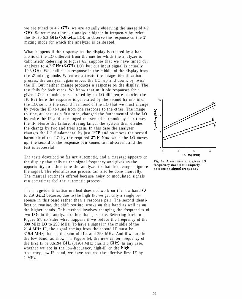
we are tuned to 4.7 GHz, we are actually observing the image of 4.7GHz. So we must tune our analyzer higher in frequency by twicethe IF, to 5.3 GHz (5.6-GHz LO), to observe the response on the l-mixing mode for which the analyzer is calibrated.

What happens if the response on the display is created by a har-monic of the LO different from the one for which the analyzer iscalibrated? Referring to Figure 65, suppose that we have tuned ouranalyzer to 4.7 GHz (5-GHz LO), but our input signal is actually10.3 GHz. We shall see a response in the middle of the display fromthe 2’ mixing mode. When we activate the image- identificationprocess, the analyzer again moves the LO, up and down, by twicethe IF. But neither change produces a response on the display. Thetest fails for both cases. We know that multiple responses for agiven LO harmonic are separated by an LO difference of twice theIF. But here the response is generated by the second harmonic ofthe LO, so it is the second harmonic of the LO that we must changeby twice the IF to tune from one response to the other. The imageroutine, at least as a first step, changed the fundamental of the LOby twice the IF and so changed the second harmonic by four timesthe IF. Hence the failure. Having failed, the system then dividesthe change by two and tries again. In this case the analyzerchanges the LO fundamental by just l*IF and so moves the secondharmonic of the LO by the required 2*IF. Now when the LO movesup, the second of the response pair comes to mid-screen, and thetest is successful.

The tests described so far are automatic, and a message appears onthe display that tells us the signal frequency and gives us theopportunity to either tune the analyzer to that frequency or ignorethe signal. The identification process can also be done manually.The manual routine‘is offered because noisy or modulated signalscan sometimes fool the automatic process.

The image-identification method does not work on the low band (0to 2.9 GHz) because, due to the high IF, we get only a single re-sponse in this band rather than a response pair. The second identi-fication routine, the shift routine, works on this band as well as onthe higher bands. This method involves changing the frequencies oftwo LOS in the analyzer rather than just one. Referring back toFigure 57, consider what happens if we reduce the frequency of the300 MHz LO to 298 MHz. To have a signal in the middle of the21.4 MHz IF, the signal coming from the second IF must be319.4 MHz; that is, the sum of 21.4 and 298 MHz. And if we are inthe low band, as shown in Figure 54, the new center frequency ofthe first IF is 3.6194 GHz (319.4 MHz plus 3.3 GHz). In any case,whether we are in the low-frequency, high-IF or the high-frequency, low-IF band, we have reduced the effective first IF by2 MHz.

3 4 5 6

LO Freq. (GHz)

Fig. 66. A response at a given LOfrequency does not uniquelydetermine signal frequency.

51

Although this method is called the shift method, we are actuallylooking for the absence of a shift to indicate that we are on thecorrect response on the correct band. To negate the downwardchange in the first IF, the first LO is also changed. If the band thatwe have selected on the analyzer uses a minus mixing mode - forexample, l- or 2- - the first LO is moved up in frequency. For the 3’and 4’ mixing modes, the first LO is moved down. Since the ap-propriate harmonic for the band selected must shift 2 MHz, theactual change to the LO fundamental is 2/n MHz, where n is theappropriate harmonic number. As noted above, there is no fre-quency shift of the displayed response when we are tuned to thecorrect response on the correct band. In all other cases there is ashift.

As with the image method, the shift method can be run automati-cally or manually. When run automatically, the HP 71200 indicateson its display whether the identified signal is in or out of band and,if the signal does not match the current tuning of the analyzer,gives us a choice of either tuning to the signal or ignoring it.

There is yet a third, totally manual identification routine. Thismethod takes advantage of the fact that in the high-frequency, low-IF band the response pairs are easily located, as in Figure 62. Thismethod works particularly well when external mixers are used formeasurements above 22 GHz. It also works well for modulated andnoisy signals. This method has us tune halfway between the tworesponses of a given pair (for example, those in Figure 62) and setthe frequency span wide enough to see both responses. Then wesimply note the indicated separation of the two responses. If theseparation is twice the IF (642 MHz), then we have chosen theband with the correct harmonic number. If the responses are closertogether than twice the IF, then they are produced on an LOharmonic higher than the harmonic utilized for the band we areon. If the indicated separation is greater than twice the IF, thenthe responses are produced on a lower LO harmonic. Once we havechosen the correct LO harmonic (by selecting a center frequencythat yields a 642-MHz separation of the response pair), we canchoose the correct response. For a minus mixing mode (l- or 2- onthe HP 71200, for example), we would select the response displayedto the right; for a plus mixing mode (3’ or 4’ on the HP 712001, tothe left.

PreselectionWe made the case for the spectrum analyzer with a wide-open frontend on the basis of a controlled measurement environment involv-ing few, if any, unknown signals. However, there are many cases inwhich we have no idea how many signals are involved or whattheir frequencies might be. For example, we could be searching forunknown spurious signals, conducting site-surveillance tests as

52

part of a frequency-monitoring program, or performing EM1 tests tomeasure unwanted device emissions. In all these cases, we could belooking for totally unknown signals in a potentially crowded spec-tral environment. Having to perform some form of identificationroutine on each and every response would make measurement timeintolerably long. Hence the need for some form of pre-filtering orpreselection.

What form must our preselection take? Referring back to Figure 60,assume that we have the image pair 4.7 and 5.3 GHz present at theinput of our analyzer. If we were particularly interested in one, wecould use a bandpass filter to allow that signal into the analyzerand reject the other. However, the fixed filter does not eliminatemultiple responses, so if the spectrum is crowded there is stillpotential for confusion. More important, perhaps, is the restrictionthat a fixed filter puts on the flexibility of the analyzer. If we aredoing broadband testing, we certainly do not want to be continuallyforced to change bandpass filters.

The solution is a tunable filter configured in such a way that itautomatically tracks the frequency of the appropriate mixing mode.Figure 66 shows the effect of such a preselector. Here we takeadvantage of the fact that our superheterodyne spectrum analyzeris not a real-time analyzer; that is, it tunes to only one frequency ata time. The dashed lines in Figure 66 represent the bandwidth ofthe tracking preselector. Signals beyond the dashed lines arerejected. Suppose we have signals at 4.7 and 5.3 GHz present at theanalyzer input. If we set a center frequency of 5 GHz and a span of2 GHz, let’s see what happens as the analyzer tunes across this

6Fi

range. As the LO sweeps past 4.4 GHz (the frequency at which it 5could mix with the 4.7 GHz input signal on its 1’ mixing mode), the ppreselector is tuned to 4.1 GHz and therefore rejects the 4.7 GHz i 4signal. Since the input signal does not reach the mixer, no mixing $occurs, and no response appears on the display. As the LO sweepspast 5 GHz, the preselector allows the 4.7 GHz signal to reach the

2

mixer, and we see the appropriate response on the display. The 5.3 3 4 5 6

GHz image signal is rejected, so it creates no mixing product to LO Freq. (GHz)

interact with the mixing product from the 4.7 GHz signal and causea false display. Finally, as the LO sweeps past 5.6 GHz, the prese-

Fig. 66. A preselector allows a signalto reach the mixer only when the

lector allows the 5.3 GHz signal to reach the mixer, and we see it analyzer is tuned to receive the

properly displayed. Note in Figure 61 that nowhere do the various signal.

mixing modes intersect. So as long as the preselector bandwidth isnarrow enough (it typically varies from 20 MHz at low frequenciesto 80 MHz at high frequencies) it will eliminate all image andmultiple responses.

The word eliminate may be a little strong. Preselectors do not haveinfinite rejection. Something in the 70- to 80-dB range is morelikely. So if we are looking for very low-level signals in the presenceof very high-level signals, we might see low-level images or mul-tiples of the high-level signals.

53

What about the low band? Most tracking preselectors use YIGtechnology, and YIG filters do not operate well at low frequencies.Fortunately, there is a simple solution. Figure 59 shows that noother mixing mode overlaps the l- mixing mode in the low-fre-quency, high-IF case. So a simple low-pass filter attenuates bothimage and multiple responses. Figure 67 shows the input architec-ture of a typical microwave spectrum analyzer.

3 GHz 3.6214 GHz

O-2.9 GHzz

CXI

- ==:Fig. 67. Front-end architecture of atypical preselected spectrumanalyzer.

Improved Dynamic RangeA preselector improves dynamic range if the signals in questionhave sufficient frequency separation. The discussion of dynamicrange in Chapter 2 assumed implicitly that both the large andsmall signals were always present at the mixer and that theiramplitudes did not change during the course of the measurement.But as we have seen, if signals are far enough apart, a preselectorallows one to reach the mixer while rejecting the others. For ex-ample, if we were to test a microwave oscillator for harmonics, a 40preselector would reject the fundamental when we tuned the ana- -50

lyzer to one of the harmonics. .- -60i --70

Let’s look at the dynamic range of a second-harmonic test of a 3-agz =-6o

GHz oscillator. In Figure 51 of Chapter 2, we suggested a second- e -90order specification for the input mixer such that a -40 dBm signal -103

at the mixer would produce a second harmonic product -70 dBc. We -110

also know from our discussion that for every dB the level of the-120

-90 -60 -70 -60 -50 40 30 aI -10 0

fundamental changes at the mixer, measurement range also Mxer Lev* (*am,

changes by 1 dB. The second-harmonic distortion curve has been Fig. 66. Extended second-order

regraphed in Figure 68 with an extended range. For this example, distortion graph.

we shall assume plenty of power from the oscillator and set theinput attenuator so that when we measure the oscillator funda-mental, the level at the mixer is -10 dBm, below the l-dB compres-sion point.

From the graph, we see that a -10 dBm signal at the mixer pro-duces a second-harmonic distortion component 40 dB down. Nowwe tune the analyzer to the 6-GHz second harmonic. If the prese-lector has 70-dB rejection, the fundamental at the mixer hasdropped to -80 dBm. Figure 68 indicates that for a signal of -80dBm at the mixer, the internally generated distortion is -110 dBc,

54

meaning 110 dB below the new fundamental level of -80 dBm. Thisputs the absolute level of the harmonic at -190 dBm. So the differ-ence between the fundamental we tuned to and the internallygenerated second harmonic we tuned to is 180 dB!

Clearly, for harmonic distortion, dynamic range is limited on thelow-level (harmonic) end only by the noise floor (sensitivity) of theanalyzer.

What about the upper, high-level end? When measuring the oscilla-tor fundamental, we must limit the power at the mixer to get anaccurate reading of the level. We can use either internal or externalattenuation to limit the level of the fundamental at the mixer tosomething less than the l-dB compression point. However, sincethe preselector highly attenuates the fundamental when we aretuned to the second harmonic, we can remove some attenuation ifwe need better sensitivity to measure the harmonic. A fundamentallevel of +20 dBm at the preselector should not affect our ability tomeasure the harmonic.2

Any improvement in dynamic range for third-order intermodula-tion measurements depends upon separation of the test tonesversus preselector bandwidth. As we noted, typical preselectorbandwidth is about 20 MHz at the low end and 80 MHz at the highend. As a conservative figure, we might use 18 dB per octave rolloffof a typical three-sphere YIG filter beyond the 3-dB point. So todetermine the improvement in dynamic range, we must determineto what extent each of the fundamental tones is attenuated andhow that affects internally generated distortion. From the expres-sions in Chapter 2 for third-order intermodulation, we have

(k(8)V,,V12V,cos[w,o - (2w, - w,>lt

and

(k(8)V,V,V,%os[w,o - (2w, - w,)lt.

Looking at these expressions, we see that the amplitude of thelower distortion component (2w, - w,) varies as the square of V, andlinearly with V,. On the other side, the amplitude of the upperdistortion component (2w, - wr) varies linearly with V, and as thesquare of V,. However, unlike the case in Figure 50 of Chapter 2,the preselector will not attenuate the two fundamental tonesequally. Figure 69 illustrates the situation in which we are tuned tothe lower distortion component and the two fundamental tones areseparated by half the preselector bandwidth. In this case the lower-frequency test tone is attenuated 3 dB; the upper test tone, 21 dB (3dB plus an additional 18 dB per octave away from center fre-quency). Since we are tuned to the lower distortion component,internally generated distortion at this frequency drops by a factorof two relative to the attenuation of v1 and equally as fast as theattenuation of V,. The improvement in dynamic range is a total of27 dB. Improvements for other signal separations appear in the

Dynamic Range Improvement

Sig. Sep Improvement(Presel Bw’s) W)

0.25 30.5 27

1 81

0 1 1 2 1 2 4 6

Bandwidths Offset

from Center

Fig. 69. Preselector attenuation andimprovement in third-orderintermodulation dynamic range.

55

table included in Figure 69. As in the case of second harmonicdistortion, the noise floor of the analyzer must be considered, too.For very closely spaced test tones, the preselector provides noimprovement, and we determine dynamic range as if the preselec-tor was not there.

The discussion of dynamic range in Chapter 2 also applies to thelow-pass-filtered low band. The only exceptions occur when aparticular harmonic of a low-band signal falls within the preselec-ted range. For example, if we measure the second harmonic of a1.5GHz fundamental, we get the benefit of the preselector whenwe tune to the 3-GHz harmonic.

Multiband TuningNot only does a preselector effectively eliminate image and mul-tiple responses, it makes tuning across wide frequency rangespractical. All HP spectrum analyzers with built-in preselectorsallow tuning across the entire preselected range in a single sweep,as shown in Figure 70A. Analyzers with microprocessors also allowspans less than the full preselected range that nevertheless involvemore than one mixing mode.

The wide frequency spans are accomplished by continuously tuningthe preselector while repeatedly retuning the LO as appropriate forthe harmonic used in the particular mixing mode. The abrupt stepsin the displayed noise floor occur because the IF gain is changed tocompensate for the changing conversion loss in the mixer as the LOharmonic changes. For all practical purposes, then, the preselectedrange becomes a single tuning band. However, continual sweepingacross the switch point between the low-pass-filtered low band andthe preselected high band is not allowed because a mechanicalswitch is used to select the band, and continual operation of the Fig. 70A.

switch would cause excessive wear.

The HP 71200 allows tuning over its entire tuning range becausethe same mixer is used on both low and high bands, and thereforeno band switch is involved. However, because it is not preselected,this wide tuning is not as useful as on a preselected analyzer. SeeFigure 70B.

Fig. 70B.

Pluses and Minuses of PreselectionWe have seen the pluses of preselection: simpler analyzer opera-tion, uncluttered displays, improved dynamic range, and widespans. But there are some minuses relative to the unpreselectedanalyzer as well.

First of all, the preselector has insertion loss, typically 6 to 8 dB.RE 3.81 Hit2 ST 1.887 BBC

This loss comes prior to the first stage of gain, so system sensitivity Fig. 70. Preselectionmakes wideis degraded by the full loss. In addition, when a preselector is spans practical.

connected directly to a mixer as shown in Figure 67, the interactionof the mismatch of the preselector (typically 2.5 VSWR) with that ofthe input mixer (typically 3 VSWR) can cause a degradation of

56

frequency response approaching ti dB. To minimize this interac-tion, a matching pad (fixed attenuator) or isolator is often insertedbetween the preselector and mixer. Sensitivity is degraded by thefull value of the pad (6 to 10 dB) or isolator (1 to 2 dB). The lowerloss of the isolator yields better sensitivity, but the better match ofthe pad yields better flatness.

Some architectures eliminate the need for the matching pad orisolator. As the electrical length between the preselector and mixerincreases, the rate of change of phase of the reflected and re-reflected signals becomes more rapid for a given change in inputfrequency. The result is a more exaggerated ripple effect on flat-ness. Architectures such as those used in the HP 8566A and B andHP 71210 include the mixer diode as an integral part of the prese-lector/mixer assembly. In such an assembly, there is minimal elec-trical length between the preselector and mixer. This architecturethus removes the ripple effect on frequency response and improvessensitivity by eliminating the matching pad or isolator.

Even aside from the its interaction with the mixer, a preselectorcauses some degradation of frequency response. In most configura-tions, the tuning ramp for the preselector and local oscillator comefrom the same source, but there is no feedback mechanism toensure that the preselector exactly tracks the tuning of the ana-lyzer. As a result, analyzers such as the HP 8566B have bothmanual and automatic preselector-peak routines, and best flatnessis obtained by peaking the preselector at each signal. The HP8562A, on the other hand, has preselector-peak values programmedinto the firmware for each GHz along the frequency range, sospecified frequency response is obtained without taking extra stepsto peak the preselector.

Wideband Fundamental MixingEven though Figure 67 is a simplified block diagram, if we look atit closely, we can find three areas for improved operation: ability tosweep across the low-band/high-band switch point, fundamentalmixing across the entire frequency range for better sensitivity, andautomatic preselector peaking for better amplitude accuracy andfaster measurements.

All three areas are addressed in the HP 71210. First of all, thisanalyzer uses a solid-state switch that is part of the preselectorcircuit to switch between the low and high bands. As a result, theHP 71210 can sweep across the switch point continuously andsimplify the analysis of spectra that straddle the switch point. Thesolid-state switch also permits continuous sweeps across the entire0 to 22 GHz frequency range.

57

Second, fundamental mixing avoids the loss of sensitivity thatresults from harmonic mixing. Fundamental mixing could beachieved by using a 3 to 22 GHz fundamental oscillator (if oneexisted). The actual scheme used in the HP 71210 multiplies the 3to 6.5 GHz LO as appropriate before it is applied to the mixer. Suchan arrangement is illustrated in Figure 71. In this case the sensi-tivity (noise floor) remains essentially constant across the entirefrequency range, as shown in Figure 72. The slight rise of the noiseat the high end of the low band results from an increased loss inthe solid-state switch.

3 GHz 3.6214 GHz

w r)c,ry,- =;;=

3-6.5

GHz

/+-CRT

The improved sensitivity gives the HP 71210 an advantage overharmonic-mixing analyzers when it comes to the measurement oflow-level signals. Perhaps more important is the potential forreduced test times. For example, at 20 GHz the HP 71210 enjoys asensitivity advantage of about 20 dB over the HP 8566B. For a testrequiring a given sensitivity, then, the resolution bandwidthselected on the HP 71210 can be one hundred times wider than thebandwidth on the HP 8566B. We know from Chapter 2 that sweeptime (for analog filters) is inversely proportional to the square ofthe resolution bandwidth. So the HP 71210 has a potential meas-urement time advantage over the HP 8566B of lO,OOO:l!

Finally, proper preselector peaking plays a role in both amplitudeaccuracy and measurement time. In an open-loop configuration,the tuning of the preselector may not exactly match that of theanalyzer. As a result, the preselector - a bandpass falter - will bemistuned to varying degrees as a function of frequency and so addto the non-flatness of the system. Stopping to optimize preselectortuning at each and every measurement point would add considera-bly to measurement time.

The HP 71210 achieves dynamic preselector peaking by including afourth YIG sphere in the same assembly that includes the threespheres used to form the preselector filter. The fourth sphere is theresonant element in a discriminator circuit. The resonant fre-quency of a YIG sphere is determined by the strength of the mag-netic field in which it is placed. All four spheres of the preselector/discriminator are placed in the magnetic field of an electromagnet.The tuning ramp of the analyzer determines the current in the coil

Fig. 71. Front-end architecture of theHP 71210 with solid-state bandswitch, fundamental mixing to 22GHz, and dynamic preselectorpeaking.

Fig. 72. Fundamental mixing acrossthe entire tuning range gives the HP71210 the same sensitivity at 22 GHzasat1GHz.

58

of the electromagnet and thus tunes the preselector/discriminator.There is a second, small coil within the preselector/discriminatorassembly to adjust the magnetic field of only the discriminatorsphere. The current in this small coil is such that the resonantfrequency of the discriminator sphere is higher than the resonantfrequency of the preselector spheres by 321.4 MHz, the first IF inthe high-frequency, low-IF range. From the tuning equation, weknow that 321.4 MHz is the frequency difference between the LOand an input signal for proper tuning of the analyzer to receivethat signal.

Since the discriminator sphere resonates at a frequency 321.4 MHzhigher than do the preselector spheres, if we can devise a scheme toadjust the current in the electromagnet to keep the discriminatorsphere resonating at the LO frequency, the preselector will be prop-erly tuned by definition. As shown in Figure 71, there is indeed afeedback mechanism between the discriminator and the maintuning coil. When the discriminator sphere resonates at the LOfrequency, there is no output, and no correction is added to thetuning ramp. Should the resonant frequency of the discriminatorsphere differ from the LO frequency, the current through theelectromagnet is not correct for the tuned frequency of the ana-lyzer, and not only is the discriminator sphere mistuned, but thepreselector is mistuned as well. But if the discriminator is mis-tuned, there is an output voltage that adds to or subtracts from thetuning ramp as appropriate to adjust the current in the electromag-net to bring the resonant frequency of the discriminator sphereback to the LO frequency. Again, because the discriminator sphereis properly tuned, the preselector is also properly tuned. Becausethis is a truly dynamic, real-time system, the preselector is alwaysproperly tuned and no other tuning or peaking mechanism isneeded.

So an architecture based on Figure 71 addresses all three areas ofimprovement suggested in reference to Figure 67.

SummaryIn this chapter we looked at harminic mixing as a means of extend-ing the frequency range of a spectrum analyzer. We found that,without some form of filtering ahead of the first mixer, the displaycan be complicated by image and multiple responses, and signalidentification might be necessary. We next introduced the preselec-tor, a tracking bandpass filter that essentially eliminates the un-wanted responses. Finally, we looked at an improved input archi-tecture that provides fundamental mixing over the entire frequencyrange, full-range sweeps, and a dynamically peaked preselector.edin reference to Figure 67.

Footnotes (Chapter 3)‘In the HP Modular Series, the display is shifted digitally in between the lo-dB IFgain steps.*Some sources can be damaged if high-level external signals are applied their outputcircuits. The preselector achieves its out-of-band rejection by reflecting the signal. Ifwe select 0 dB of input attenuation for best sensitivity when measuring harmonics,we must remember that the fundamental is almost totally reflected.

59

Glossary of Terms

Absolute Amplitude Accuracy: The uncertainty of an amplitude measurement in absolute terms,either volts or power. Includes relative uncertainties (see Relative Amplitude Accuracy) plus calibratoruncertainty. For improved accuracy, some spectrum analyzers have frequency response specifiedrelative to the calibrator as well as relative to the mid-point between peak-to-peak extremes.

Amplitude Accuracy: The uncertainty of an amplitude measurement, whether relative or absolute.

Analog Display: The case in which the analog signal information (from the envelope detector) iswritten directly to the display. Analyzers with vector displays, as opposed to raster displays, typicallyrevert to an analog display on fast sweeps in zero span even though the normal display mode is digital.

Average Noise Level: See Displayed Average Noise Level.

Bandwidth Selectivity: A measure of an analyzer’s ability to resolve signals unequal in amplitude.Also called shape factor, bandwidth selectivity is the ratio of the 60-dB bandwidth to the 3-dBbandwidth for a given resolution (IF) filter. For some analyzers, the 6-dB bandwidth is used in lieu ofthe 3-dB bandwidth. In either case, bandwidth selectivity tells us how steep the filter skirts are.

CRT Persistence: An indication of the rate at which the image fades on the display. In analyzers thatdigitize the trace (video) information before writing it to the screen, the refresh rate is high enough toprevent any flicker in the display, so short-persistence CRT’s are used. Purely analog (older) analyzerstypically use long persistence or variable-persistence CRT’s because the refresh rate is the same as thesweep rate.

Delta Marker: A mode in which a fixed, reference marker has been established and a second, activemarker is available that we can place anywhere on the displayed trace. A readout indicates therelative frequency separation and amplitude difference between the reference and active markers.

Digital Display: A mode in which trace (analog video) information is digitized and stored in memoryprior to being displayed. The displayed trace is a series of points. The number of points is a function ofthe particular analyzer. HP analyzers draw vectors between the points to present a continuous lookingtrace. The display is refreshed (rewritten from data in memory) at a flicker-free rate; the data inmemory is updated at the sweep rate.

Display Detector Mode: The manner in which the analog video information is processed prior tobeing digitized and stored in memory. See Neg Peak, Pos Peak, Rosenfell, and Sample.

Display Dynamic Range: The maximum dynamic range for which both the larger and smaller signalmay be viewed simultaneously on the CRT. For analyzers with a maximum logarithmic display of 10dB/div, the actual dynamic range (see Dynamic Range) may be greater than the display dynamicrange.

Display Fidelity: The uncertainty in measuring relative differences in amplitude on a spectrumanalyzer. On purely analog analyzers, differences must be read directly on the CRT display. Manyanalyzers with digital displays have markers, so differences are taken from stored data, and theambiguity of the CRT display is removed from the measurement.

Display Range: The calibrated range of the CRT for the particular display mode and scale factor. SeeLinear and Log Display and Scale Factor.

60

Displayed Average Noise Level: The noise level as seen on the analyzer’s display after setting thevideo bandwidth narrow enough to reduce the peak-to-peak noise fluctuations such that the displayednoise is seen as an essentially straight line. Usually refers to the analyzer’s own internally generatednoise as a measure of sensitivity and is typically specified in dBm under conditions of minimumresolution bandwidth and minimum input attenuation.

Drift: The slow (relative to sweep time) change of signal position on the display as a result of a changein LO frequency versus sweep voltage. While drift may require us to retune the analyzer periodically,it does not impair frequency resolution.

Dynamic Range: The ratio in dB between the largest and smallest signals, present at the input of ananalyzer simultaneously, that can be measured to a given degree of accuracy. Dynamic range generallyrefers to measurement of distortion or intermodulation products.

Envelope Detector: Also called a peak detector, a circuit element whose output follows the envelope,but not the instantaneous variation, of its input signal. In a superheterodyne spectrum analyzer, theinput to the envelope detector comes from the final IF, and the output is a video signal. When we putour analyzer in zero span, the envelope detector demodulates the input signal, and we can observe themodulating signal as a function of time on the display.

External Mixer: An independent mixer, usually with a waveguide input port, used to extend thefrequency range of those spectrum analyzers designed to utilize them. The analyzer provides the LOsignal and, if needed, mixer bias, and mixing products are returned to the analyzer’s IF input.

FFT (Fast Fourier Transform): A mathematical operation performed on a time-domain signal toyield the individual spectral components that constitute the signal. See Spectrum.

Flatness: See Frequency Response.

Frequency Accuracy: The uncertainty with which the frequency of a signal or spectral component is’ indicated, either in an absolute sense or relative to some other signal or spectral component. Absoluteand relative frequency accuracies are specified independently.

Frequency Range: The minimum to maximum frequencies over which a spectrum analyzer can tune.While the maximum frequency is generally thought of in terms of an analyzer’s coaxial input, therange of many microwave analyzers can be extended through use of external waveguide mixers.

Frequency Resolution: The ability of a spectrum analyzer to separate closely spaced spectralcomponents and display them individually. Resolution of equal amplitude components is determined byresolution bandwidth; of unequal amplitude signals, by resolution bandwidth and bandwidthselectivity.

Frequency Response: Variation in the displayed amplitude of a signal as a function of frequency.Typically specified in terms of +/- dB relative to the value midway between the extremes. Also may bespecified relative to the calibrator signal.

Frequency Span: The frequency range represented by the horizontal axis of the display. Generally,frequency span is given as the total span across the full display. Older analyzers usually indicatefrequency span (scan width) on a per-division basis.

61

Frequency Stability: A general phrase that covers both short- and long-term LO instability. Thesweep ramp that tunes the LO also determines where a signal should appear on the display. Any long-term variation in LO frequency (drift) with respect to the sweep ramp causes a signal to slowly shift itshorizontal position on the display. Shorter-term LO instability can appear as random FM or phasenoise on an otherwise stable signal.

Full Span: Depends upon the spectrum analyzer. For some, full span means a frequency span thatcovers the entire tuning range of the analyzer. These analyzers include single-band RF analyzers andmicrowave analyzers such as the HP 71210 that use a solid-stateswitch to switch between the low andpreselected ranges. For other analyzers, full span refers to a sub-range. For example, for a microwavespectrum analyzer such as the HP 8566B that uses a mechanical switch to switch between the low andpreselected ranges, full span may refer to either the low, non-preselected range or the high, preselectedrange.

Gain Compression: That signal level at the input mixer of a spectrum analyzer at which thedisplayed amplitude of the signal is a specified number of dB too low due just to mixer saturation. Thesignal level is generally specified for l-dB or 0.5-dB compression and is usually between - 3 and - 10dBm.

Harmonic Distortion: Unwanted frequency components added to a signal as the result of the non-linear behavior of the device (e.g. mixer, amplifier) through which the signal passes. These unwantedcomponents are harmonically related to the original signal.

Harmonic Mixing: The utilization of the LO harmonics generated in a mixer to extend the tuningrange of a spectrum analyzer beyond the range achievable using just the LO fundamental.

IF Gain/IF Attenuation: A control to adjust vertical the position of signals on the display withoutaffecting the signal level at the input mixer. When changed, the value of the reference level is changedaccordingly.

IF Feedthrough: A raising of the baseline trace on the display due to an input signal at theintermediate frequency passing through the input mixer. Generally a potential problem only on non-preselected spectrum analyzers. The entire trace is raised because the signal is always at the IF, i.e.mixing with the LO is not required.

Image Response: A displayed signal that is actually twice the IF away from the frequency indicatedby the spectrum analyzer. For each harmonic of the LO there is an image pair, one below and oneabove the LO frequency by the IF. Images usually appear only on non-preselected spectrum analyzers.

Incidental FM: Unwanted frequency modulation on the output of a device (signal source, amplifier)caused by (incidental to) some other form of modulation, e.g. amplitude modulation.

Input Attenuator: A step attenuator between the input connector and first mixer of a spectrumanalyzer. Also called the RF attenuator. The input attenuator is used to adjust level of the signalincident upon the first mixer. The attenuator is used to prevent gain compression due to high-leveland/or broadband signals and to set dynamic range by controlling the degree of internally-generateddistortion. In some analyzers, the vertical position of displayed signals is changed when the inputattenuator setting is changed, so the reference level is also changed accordingly. In HP microprocessor-controlled analyzers, the IF gain is changed to compensate for input attenuator changes, so signalsremain stationary on the CRT display, and the reference level is not changed.

Input Impedance: The terminating impedance that the analyzer presents to the signal source. Thenominal impedance for RF and microwave analyzers is usually 50 ohms. For some systems, e.g. cable

62

TV, 75 ohms is standard. The degree of mismatch between the nominal and actual input impedance isgiven in terms of VSWR (voltage standing wave ratio).

Intermodulation Distortion: Unwanted frequency components resulting from the interaction of twoor more spectral components passing through a device with non-linear behavior (e.g. mixer, amplifier).The unwanted components are related to the fundamental components by sums and differences of thefundamentals and various harmonics, e.g. fi +I- f,, 2*f1 +/- fz, 2*f, +I- f,, 3*f, +/- 2*fz, etc.

LO Emission or Feedout: The emergence of the LO signal from the input of a spectrum analyzer.The level can be greater than 0 dBm on non-preselected spectrum analyzers but is usually less than-70 dBm on preselected analyzers.

LO Feedthrough: The response on the display when a spectrum analyzer is tuned to 0 Hz, i.e. whenthe LO is tuned to the IF. The LO feedthrough can be used as a O-Hz marker, and there is nofrequency error.

Linear Display: The display mode in which vertical deflection on the display is directly proportionalto the voltage of the input signal. The bottom line of the graticule represents 0 V, and the top line, thereference level, some non-zero value that depends upon the particular spectrum analyzer. On the HP140 series of analyzers, we select a specific scale factor in V/div. On most newer analyzers, we selectthe reference level, and the scale factor becomes the reference level value divided by the number ofgraticule divisions. Although the display is linear, analyzers with microprocessors allow reference leveland marker values to be indicated in dBm, dBmV, dBuV, and, in some cases, watts as well as volts.

Log Display: The display mode in which vertical deflection on the display is a logarithmic function ofthe voltage of the input signal. We set the display calibration by selecting the value of the top line ofthe graticule, the reference level, and scale factor in dB/div. On HP analyzers, the bottom line of thegraticule represents zero volts for scale factors of 10 dB/div or more, so the bottom division is notcalibrated in these cases. Analyzers with microprocessors allow reference level and marker values to beindicated in dBm, dBmV, dBuV, volts, and, in some cases, watts.Non-microprocessor based analyzersusually offer only one choice of units, and dBm is the usual choice.

Marker: A visible indicator that we can place anywhere along the CRT trace. A readout indicates theabsolute value of both the frequency and amplitude of the trace at the marked point. The amplitudevalue is given in the currently selected units. Also see Delta Marker and Noise Marker.

Measurement Range: The ratio, expressed in dB, of the maximum signal level that can be measured(usually the maximum safe input level) to the lowest achievable average noise level. This ratio isalmost always much greater than can be realized in a single measurement. See Dynamic Range.

Mixing Mode: A description of the particular circumstance that creates a given response on aspectrum analyzer. The mixing mode, e.g. l+, indicates the harmonic of the LO used in the mixingprocess and whether the input signal is above (+) or below (-) that harmonic.

Multiple Responses: Two or more responses on a spectrum analyzer display from a single inputsignal. Multiple responses occur only when mixing modes overlap and the LO is swept over a wideenough range to allow the input signal to mix on more that one mixing mode. Normally notencountered in analyzers with preselectors.

Neg Peak: For digital displays, the display detection mode in which each displayed point indicates theminimum value of the video signal for that part of the frequency span and/or time interval representedby the point.

63

Noise Figure: The ratio, usually expressed in dB, of the signal-to-noise ratio at the input of a device(mixer, amplifier) to the signal-to-noise ratio at the output of the device.

Noise Marker: A marker whose value indicates the noise level in a l-Hz noise power bandwidth.When the noise marker is selected, the sample display detection mode is activated, the values of anumber of consecutive trace points (the number depends upon the analyzer) about the marker areaveraged, and this average value is normalized to an equivalent value in a l-Hz noise powerbandwidth. The normalization process accounts for detection and bandwidth plus the effect of the logamplifier when we select the log display mode.

Noise Sidebands: Modulation sidebands that indicate the short-term instability of the LO (primarilythe first LO) system of a spectrum analyzer. The modulating signal is noise, in the LO circuit itselfand/or in the LO stabilizing circuit, and the sidebands comprise a noise spectrum. The mixing processtransfers any LO instability to the mixing products, so the noise sidebands appear on any spectralcomponent displayed on the analyzer far enough above the broadband noise floor. Because thesidebands are noise, their level relative to a spectral component is a function of resolution bandwidth.Noise sidebands are typically specified in terms of dBc/Hz (amplitude in a l-Hz bandwidth relative tothe carrier) at a given offset from the carrier, the carrier being a spectral component viewed on thedisplay.

Phase Noise: See Noise Sidebands.

Pos Peak: For digital displays, the display detection mode in which each displayed point indicates themaximum value of the video signal for that part of the frequency span and/or time interval representedby the point.

Preamplifier: An external, low-noise-figure amplifier that improves system (preamplifier/spectrum-analyzer) sensitivity over that of the analyzer itself.

Preselector: A tunable, bandpass filter that precedes the input mixer of a spectrum analyzer andtracks the appropriate mixing mode. Preselectors are typically used only above 2 GHz. They essentiallyeliminate multiple and image responses and, for certain signal conditions, improve dynamic range.

Raster Display: A TV-like display in which the image is formed by scanning the electron beamrapidly across and slowly down the CRT face and gating the beam on as appropriate. The scanningrates are fast enough to produce a flicker-free display. Also see Vector Display and Sweep Time.

Reference Level: The calibrated vertical position on the display used as a reference for amplitudemeasurements. The reference level position is normally the top line of the graticule, but on HP 71000spectrum analyzers the reference level position may be located anywhere.

Relative Amplitude Accuracy: The uncertainty of an amplitude measurement in which theamplitude of one signal is compared to the amplitude of another regardless of the absolute amplitude ofeither. Distortion measurements are relative measurements. Contributors to uncertainty includefrequency response and display fidelity and changes of input attenuation, IF gain, scale factor, andresolution bandwidth.

Residual FIM: The inherent short-term frequency instability of an oscillator in the absence of anyother modulation. In the case of a spectrum analyzer, we usually expand the definition to include thecase in which the LO is swept. Residual FM is usually specified in peak-to-peak values because theyare most easily measured on the display if visible at all.

Residual Responses: Discrete responses seen on a spectrum analyzer display with no input signalpresent.

64

Resolution: See Frequency Resolution.

Resolution Bandwidth: The width of the resolution bandwidth (IF) filter of a spectrum analyzer atsome level below the minimum insertion-loss point (maximum deflection point on the display). For HPanalyzers, the 3-dB bandwidth is specified; for some others, it is the 6-dB bandwidth.

Rosenfell: For digital displays, the display detection mode in which the value displayed at each pointis based upon whether or not the video signal both rose and fell during the frequency and/or timeinterval represented by the point. If the video signal only rose or only fell, the maximum value isdisplayed. If the video signal did both rise and fall, then the maximum value during the interval isdisplayed by odd-numbered points, the minimum value, by even-numbered points. To prevent the lossof a signal that occurs only in an even-numbered interval, the maximum value during this interval ispreserved, and in the next (odd-numbered) interval, the displayed value is the greater of the valuecarried over or the maximum that occurs in the current interval.

Sample: For digital displays, the display detection mode in which the value displayed at each point isthe instantaneous value of the video signal at the end of the frequency span and/or time intervalrepresented by the point.

Scale Factor: The per-division calibration of the vertical axis of the display.

Sensitivity: The level of the smallest sinusoid that can be observed on a spectrum analyzer, usuallyunder optimized conditions of minimum resolution bandwidth, 0 dB RF input attenuation, andminimum video bandwidth. HP defines sensitivity as the displayed average noise level. A sinusoid atthat level will appear to be about 2 dB above the noise.

Shape Factor: See Bandwidth Selectivity.

Signal Identification: A routine, either manual or automatic, that indicates whether or not aparticular response on the spectrum analyzer’s display is from the mixing mode for which the displayis calibrated. If automatic, the routine may change the analyzer’s tuning to show the signal on thecorrect mixing mode, or it may tell us the signal’s frequency and give us the option of ignoring thesignal or having the analyzer tune itself properly for the signal. Generally not needed on preselectedanalyzers.

Span Accuracy: The uncertainty of the indicated frequency separation of any two signals on thedisplay.

Spectral Purity: See Noise Sidebands.

Spectral Component: One of the sine waves comprising a spectrum.

Spectrum: An array of sine waves of differing frequencies and amplitudes and properly related withrespect to phase that, taken as a whole, constitute a particular time-domain signal.

Spectrum Analyzer: A device that effectively performs a Fourier transform and displays theindividual spectral components (sine waves) that constitute a time-domain signal. Phase may, or maynot, be preserved, depending upon the analyzer type and design.

Spurious Responses: The improper responses that appear on a spectrum analyzer display as a resultof the input signal. Internally-generated distortion products are spurious responses, as are image andmultiple responses.

65

Sweep Time: The time to tune the LO across the selected span. Sweep time does not include the deadtime between the completion of one sweep and the start of the next. In zero span, the spectrumanalyzer’s LO is fixed, so the horizontal axis of the display is calibrated in time only. In non-zero spans,the horizontal axis is calibrated on both frequency and time, and sweep time is usually a function offrequency span, resolution bandwidth, and video bandwidth.

Units: Dimensions on the measured quantities. Units usually refer to amplitude quantities becausethey can be changed. In spectrum analyzers with microprocessors, available units are dBm (dB relativeto 1 milliwatt dissipated in the nominal input impedance of the analyzer), dBmV (dB relative to 1millivolt), dBuV (dB relative to 1 microvolt), volts, and, in some analyzers, watts. In HP analyzers, wecan specify any units in both log and linear displays.

Variable Persistence: That property of a CRT that allows adjustment of the fade rate of a tracecreated by the CRT’s electron beam. For purely analog displays. Used in the HP 141T SpectrumAnalyzer Mainframe for flicker-free displays regardless of sweep time.

Vector Display: The CRT in which the electron beam is directed so that the image (trace, graticule,annotation) is written directly on the CRT face, not created from a series of dots as in the rasterdisplay.

Video: In a spectrum analyzer, a term describing the output of the envelope detector. The frequencyrange extends from 0 Hz to a frequency typically well beyond the widest resolution bandwidthavailable in the analyzer. However, the ultimate bandwidth of the video chain is determined by thesetting of the video filter.

Video Amplifier: A post-detection, dc-coupled amplifier that drives the vertical deflection plates of theCRT. See Video Bandwidth and Video Filter.

Video Average: A digital averaging of a spectrum analyzer’s trace information. Available only onanalyzers with digital displays. The averaging is done at each point of the display independently and iscompleted over the number of sweeps selected by the user. The averaging algorithm applies aweighting factor (l/n, where n is the number of the current sweep) to the amplitude value of a givenpoint on the current sweep, applies another weighting factor [(n - 1)/n] to the previously storedaverage, and combines the two for a current average. After the designated number if sweeps arecompleted, the weighting factors remain constant, and the display becomes a running average.

Video Bandwidth: The cutoff frequency (3-dB point) of an adjustable low pass filter in the,videocircuit. When the video bandwidth is equal to or less than the resolution bandwidth, the video circuitcannot fully respond to the more rapid fluctuations of the output of the envelope detector. The result isa smoothing of the trace, i.e. a reduction in the peak-to-peak excursion of broadband signals such asnoise and pulsed RF when viewed in the broadband mode. The degree of averaging or smoothing is afunction of the ratio of the video bandwidth to the resolution bandwidth.

Video Filter: A post-detection, low-pass filter that determines the bandwidth of the video amplifier.Used to average or smooth a trace. See Video Bandwidth.

Zero Span: That case in which a spectrum analyzer’s LO remains fixed at a given frequency so theanalyzer becomes a fixed-tuned receiver. The bandwidth of the receiver is that of the resolution (IF)bandwidth. Signal amplitude variations are displayed as a function of time. To avoid any loss of signalinformation, the resolution bandwidth must be as wide as the signal bandwidth. To avoid anysmoothing, the video bandwidth must be set wider than the resolution bandwidth.

66

Index

Absolute 23accuracyAmplitude measurements 16, 18Amplitude accuracy 22,25,39,57,5&lAnalog filters 9Analog displays 18Attenuator test 38Automatic preselector peaking 57Bandwidth selectivity 10. 11Best sensitivity 25,26, 29Best dynamic range 39Calibrator 23,24Conversion loss of a mixer 25,49CRT displays 6,18CW compression 40Define dynamic range 34Digital displays 19-22Digital filters 11, 14Display smoothing 16-18Display range 5,40-41Display fidelity 22,24Display dynamic range 41Dynamic range versus noise 38Dynamic range versus measurementuncertainty 39Dynamic preselector peaking 58Dynamic range 4,34-44Dynamic range versusinternal distortion 35Effect on sweep time 13,14EMI (Electra Magnetic Interference) 3Envelope detector 15FFT (Fast Fourier Transform) 4,11Filter skirt 10Flatness 22,57,58Fourier 1,9Frequency response 22,23,57,58Frequency domain 1,2,. 3Frequency resolution 9Fundamental mixing 47-49,57,58Gaussian distribution 31Harmonic mixing 46-49,58Harmonic distortion 2,3Heterodyne 4Image pairs 50Image method 50Images 48Impedance mismatch 23Improved dynamic range 54-56Improving overall uncertainty 23-24IF (Intermediate frequency) 4,6-8Intermodulation distortion 36-37kTB24,27,29,33Linear scale 5LO residual FM 12LG feedthmugh 8,9Local oscillator frequency 6Log scale 5, 16Manual identificationMean value of a Rayleigh distribution 32Measurement uncertainty 22-23,39-40M e a s u r e m e n t 29,30,37,41,42rangeMixer compression 29,40,41Mixing product 6, 7,9, 12, 16, 21, 35,40,

46,47Multiband tuning 56

Multiple responses 48, 49, 51, 53, 54Neg peak 20-22Noise marker 33Noise signals 21, 24-25, 33, 34Noise floor 12,25,28-29, 33,34,39,49,

55, 56, 58Noise figure 2631Noise as a signal 28,31Noise-power bandwidth 29,32,34Period 1Phase 1,4, 12, 13, 39, 40,49,50, 57Phase noise 12, 13,39,49,50Pluses and minuses of preselection 56Pos peak 17,20,21,22Preamplifier 27-31,33-34Preamplifier for noise measurements 33Preselection 52-53, 56Preselector peaking 57,58Preselector bandwidth 53,55Pulse compression 4 1Random noise 12, 20, 24, 28, 31Rayleigh distribution 32-33Reference level 5,25,41-42Relative uncertainty 22-23Relative measurements 22Residual FM 12Resolution 23-26RMS value of a sinewave 28,32Rosenfell 20-22Sample mode 19-2 1Saturation 38,40Second-harmonic mixing 47Second-order distortion 37Selectivity 10, 11,13,32Sensitivity 4, 24, 25,26, 27, 28, 31, 33,

39,55-58Shape factor 10Shift method 52Sideband noise 12Signal identification 48, 59Signal-to-noise ratio 24, 25,26,27, 38-39,

40Single-band RF spectrum analyzer 8Spectral occupancy 3Storage CRT 18Superhetemdyne spectrum analyzer 1,4,

53Sweep time 13, 14,17,18,58Third-order distortion 37, 38, 39Third-order intermodulation 2,34,37Time-domain 1-2, 11TOI (Third Order intercept) 38Tuning range 6,7,35,46,47,48,49,56Tuning equation 6, 7,8, 35,46,47,59Tuning (mixing) equation 6,47Two-tone compression 41Variable-persistence 19Video bandwidth 17,26Video filtering 16, 18,26,28,29, 31,32Video averaging 17-18,28,29,31,32Wideband fundamental mixing 57

67

United States:Hewlett-Packard Company4 Choke Cherry RoadRockville, MD 20850

Hewlett-Packard Company5201 Tollview DriveRolling Meadows, IL 60008

Hewlett-Packard Company516 1 Lankershim Blvd.No. Hollywood, CA 91601

Hewlett-Packard Company2015 South Park PlaceAtlanta, GA 30339

Canada:Hewlett-Packard Ltd.6877 Goreway DriveMississauga, Ontario L4VlM8(416) 678-9430

Australia/New Zealand:Hewlett-Packard Australia Ltd.31-41 Joseph StreetBlackburn, Victoria 3130Melbourne, Australia

Europe/Africa/Middle East:Hewlett-Packard S.A.Central Mailing DepartmentP.O. Box 5291180 AM AmstelveenThe Netherlands

Far East:Hewlett-Packard Asia Ltd.22/F Bond CentreWest Tower89 QueenswayCentral, Hong Kong

Japan:Yokogawa-Hewlett-Packard Ltd.29-21, Takaido-Higashi 3-chomeSuginami-ku, Tokyo 168

Latin America:Latin American Region Headquarter1Monte Pelvoux Nbr. 111Lomas de Chapultapec11000 Mexico, D.F. Mexico

November 1,1989Printed in U.S.A.6962-0292