Spectral phase retrieval from interferometric ...sibor.physics.tamu.edu/publications/papers/2010-03.pdf · Spectral phase retrieval from interferometric autocorrelation by a combination

Spectral phase retrieval from interferometric

autocorrelation by a combination of graduated

optimization and genetic algorithms

Wenlong Yang*, Matthew Springer, James Strohaber, Alexandre Kolomenski, Hans

Schuessler, George Kattawar and Alexei Sokolov

Institute for Quantum Studies and Department of Physics & Astronomy, Texas A&M University,

College Station, TX 77843-4242 USA.

*[email protected]

Abstract: We describe a method for retrieving spectral phase information

from second harmonic interferometric autocorrelation measurements

supplemented by the use of the observed spectral intensity. By applying a

combination of graduated optimization and genetic algorithms, accurate

phase retrieval of laser pulses as short as a few optical cycles was obtained

from the measured autocorrelation and spectral intensity. The effectiveness

of the combined algorithms is demonstrated on a set of significantly

different femtosecond pulse shapes.

© 2010 Optical Society of America

OCIS codes: (320.7100) Ultrafast measurement; (320.5550) Pulses; (100.5070) Phase retrieval.

References and Links

1. J.-C. Diels, and W. Rodulph, Ultrashort Laser Pulse Phenomena, (Elsevier, 2006), chap. 9.

2. T. Trebino, Frequency-Resolved Optical Gating: The Measurement of Ultrashort Laser Pulses, (Kluwer

Academic Publishers, 2000).

3. C. Iaconis, and I. A. Walmsley, “Spectral phase interferometry for direct electric-field reconstruction of

ultrashort optical pulses,” Opt. Lett. 23(10), 792–794 (1998).

4. M. Takeda, H. Ina, and S. Kobayashi, “Fourier-transform method of fringe-pattern analysis for computer-based

topography and interferometry,” J. Opt. Soc. Am. 72(1), 156–160 (1982).

5. K. Naganuma, K. Mogi, and H. Yamada, “General Method for Ultrashort Light Pulse Chirp Measurement,”

IEEE J. of Quan. Elec. 25, 6 (1989).

6. M. Mitchell, An Introduction To Genetic Algorithms, (MIT, 1998).

7. R. S. Judson, and H. Rabitz, “Teaching lasers to control molecules,” Phys. Rev. Lett. 68(10), 1500–1503 (1992).

8. C. J. Bardeen, V. V. Yakovlev, K. R. Wilson, S. D. Carpenter, P. M. Weber, and W. S. Warren, “Feedback

quantum control of molecular electronic population transfer,” Chem. Phys. Lett. 280(1-2), 151–158 (1997).

9. T. Baumert, T. Brixner, V. Seyfried, M. Strehle, and G. Gerber, “Femtosecond pulse shaping by an evolutionary

algorithm with feedback,” Appl. Phys. B 65(6), 779–782 (1997).

10. A. Efimov, M. D. Moores, N. M. Beach, J. L. Krause, and D. H. Reitze, “Adaptive control of pulse phase in a

chirped-pulse amplifier,” Opt. Lett. 23(24), 1915–1917 (1998).

11. E. Zeek, K. Maginnis, S. Backus, U. Russek, M. Murnane, G. Mourou, H. Kapteyn, and G. Vdovin, “Pulse

compression by use of deformable mirrors,” Opt. Lett. 24(7), 493–495 (1999).

12. T. Hornung, R. Meier, D. Zeidler, K.-L. Kompa, D. Proch, and M. Motzkus, “Optimal control of one- and two-

photon transitions with shaped femtosecond pulses and feedback,” Appl. Phys. B 71, 277–284 (2000).

13. B. J. Pearson, J. L. White, T. C. Weinacht, and P. H. Bucksbaum, “Coherent control using adaptive learning

algorithms,” Phys. Rev. A 63(6), 063412 (2001).

14. F. G. Omenetto, A. J. Taylor, M. D. Moores, and D. H. Reitze, “Adaptive control of femtosecond pulse

propagation in optical fibers,” Opt. Lett. 26(12), 938–940 (2001).

15. J. W. Nicholson, F. G. Omenetto, D. J. Funk, and A. J. Taylor, “Evolving FROGS: phase retrieval from

frequency-resolved optical gating measurements by use of genetic algorithms,” Opt. Lett. 24(7), 490–492

(1999).

16. R. Mizoguchi, K. Onda, S. S. Kano, and A. Wada, “Thinning-out in optimized pulse shaping method using

genetic algorithm,” Rev. Sci. Instrum. 74(5), 2670–2674 (2003).

17. E. Carroll, A. Florean, J. L. White, P. H. Bucksbaum, and R. J. Sension, “Control of 1,3-Cyclohexadiene Ring-

Opening,” Ultra-fast Phenomena 88, 249–251 (2007).

18. C.-W. Chen, J. Y. Huang, and C.-L. Pan, “Pulse retrieval from interferometric autocorrelation measurement by

use of the population-split genetic algorithm,” Opt. Express 14, 22 (2006).

#128510 - $15.00 USD Received 17 May 2010; revised 14 Jun 2010; accepted 17 Jun 2010; published 29 Jun 2010(C) 2010 OSA 5 July 2010 / Vol. 18, No. 14 / OPTICS EXPRESS 15028

19. K.-H. Hong, Y. S. Lee, and C. H. Nam, “Electric-field reconstruction of femtosecond laser pulses from

interferometric autocorrelation using an evolutionary algorithm,” Opt. Commun. 271(1), 169–177 (2007).

20. J.-H. Chung, and A. M. Weiner, “Ambiguity of Ultrashort Pulse Shapes Retrieved From the Intensity

Autocorrelation and the Power Spectrum,” IEEE J. Sel. Top. Quantum Electron. 7(4), 656–666 (2001).

21. D. A. Bender, J. W. Nicholson, and M. Sheik-Bahae, “Ultrashort laser pulse characterization using modified

spectrum auto-interferometric correlation (MOSAIC),” Opt. Express 16(16), 11782–11794 (2008).

22. D. A. Bender, and M. Sheik-Bahae, “Modified spectrum autointerferometric correlation (MOSAIC) for single-

shot pulse characterization,” Opt. Lett. 32(19), 2822–2824 (2007).

23. A. Rosenfeld, Multiresolution Image Processing and Analysis (Springer, 1984).

1. Introduction

Measurement of ultrashort laser pulse shapes is an important non-trivial task. There are

several methods allowing for the full characterization of the electric field [1–3]; the most

common of these measuring methods include second harmonic interferometric

autocorrelation (SHIAC) [1], frequency resolved optical gating (FROG) [2] and spectral

interferometry for direct electric-field reconstruction (SPIDER) [3]. FROG uses a generalized

projection method to retrieve both the spectral phase and amplitude [1]. SPIDER uses non-

iterative calculations [4] to get the spectral phase and amplitude. Naganuma et. al. [5] have

shown that the knowledge of both SHIAC trace and spectral intensity are sufficient for pulse

reconstruction. To this end, they provided a Gerchberg–Saxton like algorithm to retrieve

spectral phases from the autocorrelation and spectral intensity measurements.

Genetic algorithms (GA) [6] are a class of universal evolutionary searching algorithms for

solving complex problems. They have been successfully used in femtosecond optics research

[7–17]. Of particular interest to the subject presented here, GAs have also found application

in the retrieval of spectral phase information from SHIAC [18, 19]. In [18], the spectral phase

of individual frequencies are used as genes, as was originally done in [7]. This method allows

the adjustment of the phase for local perturbations, but it will take many steps to compensate

a big global phase change, such as a big linear chirp and higher-order chirps. In [19], the

spectral phase is expanded in a Taylor series around the center frequency, as was originally

done in [8, 9]. This method can retrieve the linear chirp and higher-order chirps very

effectively, however, it lacks the ability to find local sharp perturbations of the spectral phase.

As is shown in [20], although SHIAC and spectral intensity are sufficient to retrieve the

spectral phase, a small difference in SHIAC may correspond to very different pulse shapes.

Therefore, in order to avoid spurious pulse shapes, a high accuracy phase retrieval algorithm

is highly desirable. The GA used in our work combines the two methods discussed above

[18,19] and is able to retrieve spectral phases with both large chirps and rapid local

perturbations.

GAs are noted for their parallel-search ability in solving multi-parameter optimization

problems and their ability to avoid local optima; although, in some pathologic cases, they too

can be trapped in a local extremum. Also, for a big parameter space, GA is very slow to

converge. Bender et al. have shown that a good starting point is helpful for an iterative

algorithm for the phase retrieval of modified spectrum auto-interferometric correlation

(MOSAIC) [21]; a sequential searching algorithm [22] has been used to seed the iterative

algorithm in their work. In our work, the graduated optimization algorithm (GOA) [23] is

employed to provide a starting point for GA. GOA as a global searching algorithm, reduces a

complex problem into a much simpler one. Then it makes a more detailed optimization in the

vicinity of the extrema of the previously simplified problem and repeats this process until the

original problem is optimized to a specified precision. In this way, GOA can search a big

parameter space and provide GA with a good starting point that is around the global optimum.

In this paper, a method is presented that combines GOA with GA so as to avoid local

extrema and reach an accurate optimization solution efficiently. We find this algorithm to be

well-suited for retrieving phase information from SHIAC and spectral intensity

measurements.


This paper is organized as follows. In Section 2, the method of the algorithms is

presented. In Section 3, the results of the algorithm implementation are shown by successfully

retrieving the phases of two experimentally available femtosecond (fs) pulses and four noise-

free simulated pulses from their SHIACs and spectral intensities. In Section 4, conclusions

and discussions are given.

2. Method

To obtain the spectral phase of a short pulse, the GOA is used to make a rough estimate of the

spectral phase and the GA is then employed to fine-tune the spectral phase to reach the

desired accuracy.

The spectral phase of a short pulse can roughly be expressed in a polynomial form:

2 3 4

2 0 3 0 4 0( ) ( ) ( ) ( ) ,

pa a aϕ ω ω ω ω ω ω ω= − + − + − (1)

where 0

ω is the central angular frequency and i

a (i = 2, 3, 4) are chirp parameters.

Commonly, these parameters contribute most to the non-trivial part of the spectral phase. The

constant and linear part of the spectral phase 0 1 0

( )a a ω ω+ − are omitted in Eq. (1) because

they are the absolute phase and delay, which are not determined by autocorrelation

measurements. Values of i

a (i = 2, 3, 4) of the spectral phase are first coarsely searched by

the GOA over i

a ’s whole parameter space. In fact, there are higher-order expansion terms, or

in other words, more local details in the spectral phase that cannot be described by these three

parameters. That is why we use the GA to find the details of the spectral phase and make fine

tunings of the i

a . Before giving a detailed description of the algorithm, the definition of the

problem and the data preparation are described in the following subsection. The algorithms

are described in later subsections.

2.1 Description of problem and data preparation

In reference [5], it was shown that the measured SHIAC ( )ac

I τ together with the spectral

intensity 2

( )E ωɶ can uniquely determine the spectral phase of an ultrafast pulse. This is the

basis of our algorithm.

The first step of our algorithm is to prepare the data. In order to compensate for the linear

distortion of the measured SHIAC, ( )ac

I τ is modified to _

( )ac inuse

I τ

_

( ) ( ),ac inuse ac

I I bτ τ= (2)

where b can be determined initially by visually matching the Fourier transform of _

( )ac inuse

I τ

and the measured spectral intensity, as was explained in reference [5]. The GA will be used to

refine this parameter later. A given ( )ϕ ω and the measured spectral intensity can be

employed to calculate the pulse shape. The pulse shape is subsequently used to calculate the

autocorrelation_

( )ac cal

I τ . The difference between _

( )ac cal

I τ and _

( )ac inuse

I τ is described by

the root mean square (rms) error ∆ :

2

_ _

1

( ) ( ) / ,N

ac cal i ac inuse i

i

I I Nτ

ττ τ=

∆ = − ∑ (3)

where Nτ is the number of sampled points of τ . This error can be understood as the average

difference between the retrieved SHIAC and the measured or simulated SHIAC. The units of

the rms error ∆ are the same as the units of SHIAC, whose peak is chosen to be 1. The GOA

+ GA combined algorithm was designed to minimize ∆ .


2.2 Graduated optimization algorithm

In our program, i

a were optimized one by one. The time unit was fs and the angular

frequency unit was rad/fs. Thus 2

a , 3

a , and 4

a have units of (fs/rad)2, (fs/rad)

3 and (fs/rad)

4

respectively. When optimizing 2

a , we set 3

a and 4

a to zero. For example, we searched 2

a

from 0 to 100 with a step size of 10. In this way, we were able to find a minimum within a

region of 20. Then we reduced the step size to 1 and search this smaller region. The one

giving minimum error is called 2 _ opt

a . Next, we set 2

a to 2 _ opt

a , 4

a to zero and gradually

optimized 3

a . After we obtained 3_ opt

a , we set 2

a to 2 _ opt

a , 3

a to 3_ opt

a and obtained 4 _ opt

a

by the same procedure. These optimized _i opt

a were used as starting values in the GA. The

range of the searching process may differ from one experiment to another. The general rule is

that these numbers must be set large enough to guarantee the optimization of i

a to give a

global minimum of ∆ and they must not be so large that the calculated pulse is too long to be

characterized by SHIAC. This searching sequence was also used in phase retrieval from

MOSAIC in ref [22].

2.3 Genetic algorithm

The GA belongs to the class of evolutionary algorithms. It was inspired by natural

evolutionary biology and is commonly used in multi-parameter optimization problems.

Generally, an optimization problem is to extremize a fitness function by tuning its variables.

In GA, the variables form a genome where each variable is a gene. Each gene can vary in a

certain range. A generation is formed by individuals whose genes have different values.

Fitness values are calculated for individuals from the fitness function. Only those with the

extreme fitness values will survive, and they are called parents. Parents will produce the next

generation using the following three methods: 1) inheritance, a process in which parents

transfer their genes to their children (individuals of the next generation) without any change

in the genes’ value; 2) mutation, a process in which parents pass somewhat modified genes to

their children; 3) crossover, which means that parents’ genes are combined to form the

genome of their children. As the next generation is produced, they will go through the process

of selection and produce another next generation. In this way, individuals in later generations

on average have better fitness values. The problem is thus optimized by the evolutionary

process, which proceeds toward “survival of the fittest”.

Most pulse spectra can be considered as distributed in a finite frequency region; namely

start endω ω ω< < . We took Nω equally spaced points

iω from

startω to

endω , and ( )

rϕ ω was

the interpolation function of ( )r i

ϕ ω . Our GA’s goal is to optimize the phase ( )r

ϕ ω and

polynomial phase ( )p

ϕ ω so that the total phase ( ) ( ) ( )r p

ϕ ω ϕ ω ϕ ω= + will minimize the rms

error ∆ in Eq. (3).

Since we have already found roughly a spectral phase close to a global minimum of

∆ from the GOA, with this starting point of GA, we are more confident that the GA would

not stagnate at a local minimum. However, in order to optimize the result globally, i

a are

also used as optimization parameters. This makes the spectral phase of i

ω not only change

independently, but also collectively. This also fits the physical situation well, because when

pulses are transmitted through optics such as windows or lenses, the change of phase can be

well represented by i

a . Thus, our GA’s parameters are the combination of the parameters of

GAs used by Chen et. al. [18] and by K.-H. Hong, et al. [19]. Furthermore, in order to

optimize b in Eq. (2), a shift parameter r of the spectrum 2

( )E ωɶ is introduced in the GA.

For generation g and individual i, the phase is calculated by


( , ) ,( , ) 2,( , ) 3,( , ) 4,( , ) ,( , )

( ) ( , , , ) ( ),g i p g i g i g i g i r g i

a a aϕ ω ϕ ω ϕ ω= + (4)

where the ,( , )

( )r g i

ϕ ω was the interpolation function of ,( , )

( )r g i j

ϕ ω . Then the electric field was

obtained by

( , ) ( )

( , ) ( , )( ) ( ) .g ii i t

g i g iE t E r e e dϕ ω ωω ω= +∫ ɶ (5)

The SHIAC was calculated according to

2

2

_ ( , ) ( , ) ( , )( ) ( ) ( ) .ac cal g i g i g iI E t E t dtτ τ∞

−∞

= − + ∫ (6)

Thus, the rms error can be obtained

2

( , ) _ ( , ) _

1

( ) ( ) / ,N

g i ac cal g i i ac inuse i

i

I I Nτ

ττ τ=

∆ = − ∑ (7)

where Nτ is the number of total sample points in the error calculation. Equation (7) is the

same as Eq. (3), except that (g,i) is added as subscript to indicate the numbers of generation

and individual. ( , )g i

∆ was used as a criterion for judging which individual could survive in

GA.

In summary, ,( , )

( )r g i j

ϕ ω , 2,( , )g i

a , 3,( , )g i

a , 4,( , )g i

a and ( , )g i

r are the genes in our GA. We

call them ,( , )k g i

x . Our goal of GA is to adjust ,( , )k g i

x to minimize the fitness function ( , )g i

∆ .

Figure 1 shows the scheme of our GA.

Fig. 1. The scheme of the GA. Each parent will reproduce itself as one of the individuals in the

next generation without any change to genes, which is called inheritance. Each of them also

produces a certain number of individuals of the next generation by mutation and crossover.


3. Results

3.1. Results for experimentally available pulses

As the first example of GOA + GA, we retrieved the spectral phase of a sub-10 fs pulse

generated by a mode-locked Ti:Sapphire oscillator (FemtoLasers, Rainbow). The SHIAC was

measured by a commercial interferometric autocorrelator (FemtoLasers, 5 – 150 fs). The

spectral intensity was measured by an Ocean Optics spectrometer (550 – 1050 nm). In the

computation, each pulse is characterized by 2048 points; the time step we used was 0.25 fs,

and the time window was 512 fs.

In the GOA, 2

a was scanned from 0 to 500, 3

a from −1000 to 1000 and 4

a from −1000

to 1000. The numbers we chose above are more or less arbitrary. This process takes about 6.6

seconds on a computer with Intel® Core 2 Duo E8400 CPU. After the graduated

optimization, the retrieved SHIAC and the measured SHIAC (after data preparation) are

shown in Fig. 2 (a). There are still visible discrepancies between them.

For GA, we used the following parameters: the number of individuals 50, the number of

parents 5, children produced from inheritance 1, mutation 7, and crossover 2, the number of

generations 200, a mutation rate of 10% and a crossover rate of 25%. The mutation process is

like this: with 10% mutation rate, 10% of a parent’s genes will change their values and form

an individual of the next generation. The process of crossover is like this: with crossover rate

of 25%, a parent takes 75% of its genes and combined with 25% genes from other parents to

form an individual of the next generation. The spectral phase was sampled by Nω = 80

points. The choice of Nω is discussed in sSection 4. The GA was programmed with parallel

computing function and took about 413 seconds on the same computer (described above). The

result of the GOA + GA is shown in Fig. 2. Black dotted curve in (a) and (b) are measured

SHIAC after data processing. The red solid curve in (a) is the calculated SHIAC with the

spectral phase obtained from GOA coarse global search. The red solid curve in (b) is the

calculated SHIAC from the spectral phase obtained by GA. Measured spectral intensity and

retrieved spectral phase from GOA and the GA after GOA are shown in (c). The error of each

individual was calculated by Eq. (7) and the minimum of errors of individuals in each

generation was plotted in Fig. 2 (d).

As a second example, we sent the pulse, described above, through a thin solution of an

infrared absorber contained between two cover slips. The infrared absorber is Exciton NP800

and the solvent is 1,1,2,2-tetrachloroethane. The infrared absorber has a very strong

absorption peak around 800 nm. After the pulse transmitted through the absorber and cover

slips, its spectral intensity around 800 nm is greatly reduced due to the absorption of the

absorber, and the spectral phase is also modified due to the dispersion from the absorber and

the cover slips. The pulse’s spectral phase and intensity are more complicated than those in

the first example which provides a challenging test of our combined algorithms. In the GOA,

2a was scanned from 0 to 500.

3a was scanned from −1000 to 1000. We scanned

4a from

−5000 to 5000. These numbers are also more or less arbitrary. Parameters used in the GA

were the same as those used in example 1. The computation time for GOA was about 6.9

seconds and the GA took about 407.8 seconds to finish. The result is shown in Fig. 3. It can

be seen from Fig. 3 (b) that the retrieved SHIAC matched the experimental SHIAC quite

well.


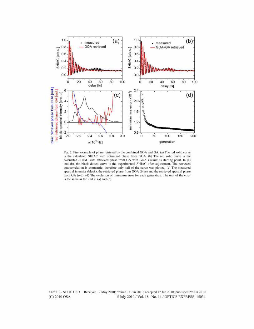
Fig. 2. First example of phase retrieval by the combined GOA and GA. (a) The red solid curve

is the calculated SHIAC with optimized phase from GOA. (b) The red solid curve is the

calculated SHIAC with retrieved phase from GA with GOA’s result as starting point. In (a)

and (b), the black dotted curve is the experimental SHIAC after adjustment. The retrieved

autocorrelation is symmetric, therefore only half of the curve was plotted. (c) The measured

spectral intensity (black), the retrieved phase from GOA (blue) and the retrieved spectral phase

from GA (red). (d) The evolution of minimum error for each generation. The unit of the error

is the same as the unit in (a) and (b).


Fig. 3. Second example of phase retrieval by the combined GOA and GA. (a) The red solid

curve is the calculated SHIAC with optimized phase from GOA. (b) The red solid curve is the

calculated SHIAC with retrieved phase from GA with GOA’s results as starting point. In both

(a) and (b), the black dotted curve is the experimental SHIAC after adjustment. The retrieved

autocorrelation is symmetric, therefore only half of the curve was plotted. (c) The measured

spectral intensity (black), the retrieved phase from GOA (blue) and the retrieved spectral phase

from GA (red). (d) The evolution of minimum error for each generation. The unit of the error

is the same as the unit in (a) and (b).

Using the inverse Fourier transform, we can calculate the retrieved electric field (Fig. 4)

from the measured spectral intensity and the retrieved spectral phase. As is expected, the

center peak of the electric field ( )E t is sharp and strong. However, the tails, which are

expected to be weak, are stronger than expected. This will be explained in the discussion part

in Section 4.

Fig. 4. (a) Retrieved electric field from combined GOA + GA in example 1. (b) Retrieved

electric field from combined GOA - GA in example 2.


GOA + GA’s results are listed in Table 1. GOA

∆ is the minimum rms error achieved by

GOA and _i opt

a are chirp parameters for the optimized pulse shape of GOA. b is defined by

Eq. (2). GOA GA−∆ is the minimum rms errors achieved by GOA + GA. However, GA’s results

ia are not very meaningful, because the spectral phase is a combination of low order chirps

and phases for individual frequencies. For example, the optimized spectral phase in Fig. 2 (c)

looks noisy and cannot be well described by i

a . We list the i

a here just to show that our GA

can fine-tune i

a and r .

Table 1. Results of GOA and GOA + GA for example 1 and 2

Results for example 1 in section 3.1

GOA’s results GOA + GA’s results

2 _ opta

3_ opta

4 _ opta *b GOA

∆ 2

a 3

a 4

a r GOA GA−∆

22 −182 194 1.04 2.2 × 10−2 22 −90.28 194 0 9 × 10−3

Results for example 2 in Section 3.1

GOA’s results GOA + GA’s results

2 _ opta

3_ opta

4 _ opta *b GOA

∆ 2

a 3

a 4

a r GOA GA−∆

33 653 −1877 1.04 4.5 × 10−2 33 653.48 −1878.4 −0.0055 2.3 × 10−2

* b is not obtained from GOA.

The necessity of GOA can be shown by comparing the results of GA with and without

GOA on both examples in this section. We applied the GA with and without the help of the

GOA six times for each example, and the minimum errors for each generation in the six runs

are shown in Fig. 5. For the GA without GOA, the starting individuals have random phases.

For example 1 (Fig. 5(a)), the average error at 50th

generation of GOA + GA is the same as

the average error of 56th

generation of GA without GOA. (Here, the average means the

average of the minimum errors of the six runs.) The computation time for one generation is

about 2.1 seconds and the GOA takes 6.6 seconds. So GOA + GA leads GA without GOA by

5.8 seconds. In Fig. 5(a), the chirp of the pulse is small, thus the GA without GOA catches up

with the GA with GOA after a couple of generations, which also shows the strong searching

ability of our GA. For example 2 (Fig. 5(b)), GA without GOA’s average error at 200th

generation is the same as the average error of GOA + GA at 106th generation, which means

GA without GOA lags GOA + GA by 188 seconds. The error of GOA with GA at 100th

generation is close to the error of GOA + GA at 70th

generation, which means GA without

GOA lags GOA + GA by 60 seconds. In this example, because the pulse has a bigger chirp,

GOA + GA is much faster than GA without GOA.

Fig. 5. (a) Comparison of GA with and without GOA with the data in example 1. (b)

Comparison of GA with and without GOA with the data in example 2. The unit of the errors is

the same as the unit of (a) and (b) in Fig. 2 and Fig. 3. The scales of (a) and (b) are made

different due to the different ranges of the data.


3.2. Results for noise-free simulated pulses

The strength of GOA + GA can be better shown by using GOA + GA to retrieve the spectral

phase of noise-free simulated pulses. An 800nm 40 fs transform limited pulse was used as the

seed pulse. Arbitrary chirps (2

a , 3

a and 4

a ) were added to the seed pulse and GOA + GA

was then used to retrieve the spectral phases of them.

For a pulse with only linear chirp 2

483a = the GOA gave exact value of the chirp with

zero error, this is as expected because GOA starts from searching 2

a , so if the pulse has only

linear chirp, GOA can find the chirp with zero error. The results of another three simulated

pulses are listed in Table 2. From the data in Table 2, the GOA + GA can make a retrieve

with error between 310− to 410− on these noise-free simulated pulses. The i

a retrieved by GA

is not listed here because the total phase is the sum of the polynomial part and the phase for

individual frequencies.

Table 2. GOA + GA’s results for noise-free simulated pulses

Pulse 1’s parameters GOA’s results GOA + GA’s results

2a

3a

4a 2 _ opt

a 3_ opt

a 4 _ opt

a GOA

∆ GOA GA−∆

23 120 1532 48 17 64 9.3 × 10−4 3.1 × 10−4

Pulse 2’s parameters GOA’s results GOA + GA’s results

2a

3a

4a 2 _ opt

a 3_ opt

a 4 _ opt

a GOA

∆ GOA GA−∆

135 −1563 −2831 132 −1420 −1908 1.2 × 10−3 1.6 × 10−4

Pulse 3′s parameters GOA’s results GOA + GA’s results

2a

3a

4a 2 _ opt

a 3_ opt

a 4 _ opt

a GOA

∆ GOA GA−∆

135 563 −11953 68 −292 −116 2.5 × 10−3 1.04 × 10−3

3.3. About the usefulness of crossover

Crossover is considered as one of the most important features of GA. It is worthy to study

how helpful crossover process is in phase retrieval problems. We ran the GA without

crossover six times and the minimum errors of each generation of the six runs are plotted in

Fig. 6 together with those of the six GA runs with crossover. We found that there is no big

difference whether we use crossover or not in GA in our phase retrieval problem.

Fig. 6. GA with and without crossover. The red dashed lines are the minimum errors of each

generation in the six runs of GA without using crossover and the black solid line are that of

GA with crossover. There is no obvious difference between the results of GA with or without

crossover. There is an unlucky case in the GA with crossover whose minimum errors are

higher than those of any other runs.


4. Conclusions and discussion

The GOA + GA combined algorithm can effectively avoid local extrema and retrieve the

spectral phase from the SHIAC and spectral intensity successfully. Chirp parameters i

a were

introduced into our GA, which strengthened the ability of our GA to search for global

extrema. For the noise-free simulated strongly chirped pulses, the rms errors between

retrieved SHIAC and the simulated SHIAC can reach 310− to 410− . For the experimentally

available pulses, errors around 210− are achieved. For pulses with small chirp parameters, the

GA itself works as well as GOA + GA. For pulses with big chirps the GOA + GA converges

faster than GA without GOA. The crossover is not found to play an important role in our GA.

There are several issues that need to be noticed. (1). Due to time reversal invariance, it is

impossible to know the sign of the total phase; thus, we defined2

a to be a positive number

and 3

a and 4

a were scanned from negative to positive numbers. (2). Due to the Nyquist–

Shannon sampling theorem, Nω determines the pulse’s temporal length that can be retrieved

accurately. However, increasing Nω will also decrease the step size used in the discrete

Fourier transform, which will increase the runtime of the algorithm. In our experiment, we are

mainly interested in the central part of the pulse and the measured SHIAC is between −100fs

to 100fs, so 80 points is sufficient for our application. However, this will cause the retrieved

electric fields (see Fig. 4.) to have some spurious tails. (3). GA is highly parallelizable. The

parallelized program is about 25% faster than serial program on the dual core computer

described in the second paragraph of Section 3.1. With multi-core computers, the parallelized

program should be faster. However, the communication between CPUs also takes time; thus,

the efficiency of this program on multi-core computer needs further investigation. (4). The

correction of the SHIAC data is crucial to the successful retrieval of the spectral phase. The

spectrum was not only a set of data that was used in the algorithm, but was also used as a

criterion to prepare the SHIAC data. We corrected only the linear shift of the SHIAC. (5).

The GOA can also be done more than once by using optimized i

a instead of zeros as starting

values. (6). As is easily notice in Fig. 5 and Fig. 6, one set of err for GOA + GA converges

slower than all others. It can be regarded as an unlucky case, which shows that luck can also

affect the result of GA. (7). Given the spectral intensity, our GOA + GA combined algorithm

provides a general method to retrieve spectral phase from measured data, and could be used to

retrieve spectral phase from FROG or MOSAIC. In order to retrieve the phase from another

kind of measurement, one only needs to change the error function to be the difference

between the calculated result and measured results.

Acknowledgments

We thank Benjamin D. Strycker, Chao Wang, Yongrui Wang for helpful discussions. We

thank the support from the Office of Naval Research (ONR) under contract N00014-08-1-

0037 and the Defense University Research Initiative Program (DURIP) under contract

N00014-08-1-0804, the National Science Foundation (NSF) (PHY 354897, 0555568 and

722800), the Texas Advanced Research Program (010366-0001-2007), the Army Research

Office (W911NF-07-1-0475), the Air Force Office of Scientific Research (FA9550-07-1-

0069) and the Robert A. Welch Foundation (A1546 and A1547).


Documents

Spectral phase retrieval from interferometric ...sibor.physics.tamu.edu/publications/papers/2010-03.pdf · Spectral phase retrieval from interferometric autocorrelation by a combination