SPECTRAL AND STATISTICAL CHARACTERISTICSCF SHCALINC WAVES DFF ALLEPPEY­

WEST CDAST CF INDIA

mesns SUBMITTED TO THE

cocu-um umvensnv or SCIENCE AND TECHNOLOGY

FOR THE DEGREE OF

DOCTOR OF PHILOSOPHYm

PHYSICAL OCEANOGRAPHY

UNDER THE FACULTY OF MARINE SCIENCES

by

.T. S. SHAHUL HAMEEDCENTRE FOR EARTH SCIENCE STUDIES

COCHIN - 682 018

MARCH 1939

DECLARATION

I do hereby declare that this Thesis contains resultsof research carried out by me under the guidance ofDr. M.Baba, Head, Centre for Earth Science Studies, Regional

Centre, Cochin, and has not previously formed the basis ofthe award of any degree, diploma, associateship, fellowshipor other similar title of recognition.

Ernakulam,Regional Centre27.3.1989. Centre for Earth Science StudiesCochin - 682 018

CERTIFICATE

This is to certify that this Thesis is an authenticrecord of research work carried out by Mr. T.S.Shahu1 Hameedunder my supervision and guidance in the Centre for EarthScience Studies for Ph.D. Degree of the Cochin University ofScience and Technology and no part of it has previouslyformed the basis for the award of any other degree in anyUniversity.

Dr. M. BABA(Research Guide)Ernakulam, Head,27.3.1989. Regional Centre

Centre for Earth Science StudiesCochin - 682 018

ACKNOWLEDGEMENTS

I am immensely grateful to Dr. M. Baba, Head, Centre for EarthScience Studies, Regional Centre, for the valuable guidance, constantencouragement and critical scrutiny of the manuscript. But for his richknowledge of the topic and vast experience, this work wouldn't havetaken this shape.

I express my deep sense of gratitude to Dr. M. Ramakrishnan,Director, and Dr. Harsh K. Gupta, former Director, Centre for EarthScience Studies, for the encouragement and the facilities extendedduring their respective terms.

I owe much to Dr. N.P.Kurian for helping me in the various stagesin the preparation of this thesis and for the useful and timelydiscussions. Thanks are‘due to my colleagues, S/Shri. K.V.Thomas, C.M.Harish and Joseph Mathew who have been of much help to me in thesuccessful completion of this work. The help rendered by Smt. SreekumariKesavan, Smt. N.Santa, S/Sri. S.Mohanan, Jomon Joseph, Shaji Joseph,Subhas Chandran, D. Baijumon and K.U. Joy during various stages of thiswork is thankfully acknowledged.

S/Shri K.K.Varghese, A.Varkey Babu, M.Ramesh Kumar, and Asokan Andyhave contributed much in making the wave recording a success. Thanks aredue to the staff of the Regional Centre, Centre for Earth ScienceStudies, who have been of help to me in one way or other during thecourse of this investigation.

The Director, Naval Physical and Oceanographic Laboratory and theScientist—in-charge, Regional Centre, National Institute of Oceano­graphy, Cochin are thanked for sparing the computer facilities availablewith them for the preparation of this thesis. S/Sri. P. Udaya Varma, C.Ravichandran, Dr. Basil Mathew and Sri. Sanal Kumar deserve specialmention for the timely help provided to me.

Finally, I must thank my wife, Asuma, who made it possible for meto concentrate on this research without being saddled by the householdaffairs.

CONTENTSPreface ,,,,, 1List of symbols ..... ivList of abbreviations ..... viiChapter 1. INTRODUCTION ..... 1Chapter 2. SPECTRAL AND STATISTICAL CHARAC­

TERISTICS OF OCEAN WAVES-A REVIEW ..... 52.1. Wave Spectrum ..... 52.2. Deep Water Wave Spectra|Models ..... 82.2.1. Phillips‘ Spectrum ..... 82.2.2. Pierson-Moskowitz Spectrum ..... 92.2.3. JONSWAP Spectrum ..... 102.2.4. Neumann Spectrum ..... 112.2.5. Darbyshire Spectrum ..... 122.2.6. Bretschneider Spectrum ..... 122.2.7. Scott and Scott-Weigel Spectra ..... 132.2.8. Toba's Model ..... 152.3. Shallow Water Spectral Models ..... 162.3.1. Kitaigorodskii et al. Spectrum ..... 172.3.2. Thornton's Model ..... 182.3.3. Jensen's Modification ..... 192.3.4. Shadrin's Model ..... 192.3.5. TMA Spectrum ..... 202.3.6. Wallops Spectrum ..... 222.3.7. GLERL Spectrum ..... 252.4. Statistical Characteristics ..... 272.5. Distribution of Wave Heights ..... 292.5.1. Rayleigh Distribution ..... 302.5.2. G1uhovskii's Distribution ..... 332.5.3. Ibrageemov's Distribution ..... 342.5.4. Truncated Rayleigh Models ..... 35, 2.5.5. Weibull Distribution ..... 372.5.6. Tayfun's Distribution ..... 382.6. Joint Distribution ..... 412.6.1. Rayleigh Distribution ..... 412.6.2. G1uhovskii's Distribution ..... 422.6.3. Longuet-Higgins Distributions ..... 442.6.4. CNEXO Distribution ..... 462.6.5. Tayfun's Distribution ..... 492.7. Summary ..... 50

Chapter 3. WAVE RECORDING AND ANALYSIS ..... 533.1. Location -.--- 533.2. Wave Recording System ..... 543.2.1. Selection of Recording System ..... 543.2.2. The Recording System Used ..... 553.2.3. Transducer Installation ..... 573.2.4. Calibration ..... 583.3. Recording Proceduresand Screening of Records ..... 59

Chapter

Chapter

0000

0 000 O\U1.hL»)t\)b—-| 00000

0. 0g 0 0

mcnoxmcnoxowmcnuwmtnu1mLnu1b

..Q. C .0

wmmmmmmra 0.0. O. OLQL»)L».)UJbQUJLA)LA)LA)UQLQLA)U)L.QLA)LA)UJ O 0 O O O

0 00

Lnv-§UJl'\.)""' no on

0

{\_)l-‘ o 0

~13-bJ>~»h.t:-1>~.b4>~.b»b.b.h.bJ=-4:-b4=~4>-£=~.bnh

0g O0 0;

~qJxmchoxwtnunfifiswtuoamnonamromJH 0 0 0 00 O0 0 O0

Lu[\_)I-0 L.oJ[\_)}-‘ O0 0 O O O

U1-I:-L;ul\)'r—I Q00 00

Preliminary AnalysisWave Climate at AlleppeyWave HeightZero-crossing PeriodWave DirectionSpectral WidthPersistence of Waves and CalmDiscussion on the Wave ClimateDetailed AnalysisSelection of RecordsSpectral AnalysisDigitization and ProcessingSpectral WindowPressure AttenuationSpectral ParametersSmoothingWave-by-Wave Analysis

OBSERVED WAVE CHARACTERISTICSObserved SpectraObserved Spectral ParametersSignificant Wave HeightPeak PeriodsSlope of the High Frequency SideSpectral WidthSpectral PeakednessAverage SpectraMonthly Average SpectraSpectra at Height—Period RangesRelation Between Spectral Parameters...Parameters from Wave-by-Wave Analysis..HeightPeriodsSpectral WidthRelation Between the ParametersWave HeightWave PeriodsSpectral WidthConclusions

WAVE SPECTRAL MODELSDerivation of a Shallow Water Model ...Comparison with ModelsJensen's ModelTMA Spectrum with Phillips‘and Average JONSWAP ParametersTMA Spectrum with Scale FactoraQand Average JONSWAP ParametersTMA Spectrum in Original FormTMA Spectrum with {Q and DerivedWallops SpectrumScott SpectrumScott-Weigel SpectrumPMK Spectrum

Constant

v°'.IZ

5962626363646465676767686970707172

757577787981848790919495

101101102104105106107108110

112112114116

117

118119121122123124125

Chapter

Chapter

5.2.10.5.3.

5.4.5.5.

6.6.16.1.1.6.1.1.1.6.1.1.2.6.1.1.3.6.1.1.4.6.1.1.5.6.1.1.6.6.1.1.7.6.1.1.8.6.1.2.6.2.6.2 1.6.2.1.1.6.2.1.2.6.2.1.3.6.2.2.6.3.

6.3.1.6.3.1.1.6.3.1.2.6.3.1.3.6.3.1.4.6.3.1.5.6.4.

7.

7.1.7.2.

GLERL ModelComparison of Average Spectrawith ModelsA Discussion on Scale Factor .....Conclusions .....HEIGHT AND PERIOD DISTRIBUTION MODELS..Distribution of Zero-crossing Heights..Comparison with Models .....Rayleigh Distribution ....Goda's ModelWeibull DistributionGluhovskii's Model . .Ibrageemov's Model ....Tayfun's ModelLonguet-Higgins’CNEXO ModelsComparison of Distribution in

Models .::.H -T Ranges with Models .....Distribution of Zero-crossing Periods..Comparison with Models .....Rayleigh Models .....Tayfun's Model .....CNBXO Models .....Comparison of Distribution inH -T Ranges with Models .....Joint Distribution ofHeights and Periods .....Comparison with Models .....Rayleigh Model .....Gluhovskii's Model .....Tayfun's Model .....CNEXO Models .....Longuet-Higgins‘ Models .....Conclusions .....SUMMARY, CONCLUSIONS ANDRECOMMENDATIONS .....Summary and Conclusions .....Recommendations for Further Research...

REFERENCES coco­APPENDIX-A .....0 0 0 0 0APPENDIX-C -oo-o

127

127130132

135135136137138140141142143145147

149154154155157158

159

160160161162163164166167

171171180

183

196

202

208

PREFACE

Waves in the oceans generated by the continuousinteraction of the winds and the ocean surface, fascinatedman's curiosity since time immemorial. The numerous hazardsdue to the ocean waves, which at times attain heights of afew tens of metres, were of concern to navigators and har­bour engineers. There is an increasing awareness in recenttimes about the importance of the study of ocean waves,because of the tremendous force exerted by waves on off­shore, harbour aumi coastal structures, their' influence ondefence, commercial and industrial operations and theirimportance in weather prediction, remote sensing and otherscientific applications. Among the useful aspects of oceanwaves are their capability to provide electric power, toenhance sediment deposition/removal as desired, to enhancebreeding of fish under controlled conditions, etc. Conside­rable efforts are being put now-a-days by oceanographers andengineers to understand the ocean waves right from theirgeneration to their dissipation.

As most of the cmean-related developmental activitiesare confined to the coastal waters the study of waves inshoaling waters is of vital importance. Unlike deep waterwaves, those in shallow waters exhibit complex characteris­tics due to non-linearities caused‘by various processes likeshoaling, frictional attenuation, refraction, diffraction,wave-wave interaction, etc., observed during the propagationof the waves to the shore.

The random waves in time ocean are not amenable tosimple mathematical explanation due to the large number ofparameters involved auui their" complex nature. Hence thesewaves are often described in terms of their spectral andstatistical characteristics. Among the above two, the spec­tral characteristics stand first, as the spectrum providesinformation on the energy contained in the component freque­ncies. It also reveals the existence of different wavesystems. This information is requinaj for studies such asharbour resonance, wave forces on structures, wave powergeneration, and many others. The spectral function is impor­tant not only due to its own information content, but alsobecause of the fact that various statistical measures of theocean surface wave field are expressed either in terms of oras quantities derived from the spectrum. The statisticalparameters depict the randomness of surface wave field.Among the various statistical measures the probability

density functions of the surface elevati0H: 995104 d”d theér. . , 9 0 I , ' ) "Jdlflt distribution are the 0dSlC ones. The Pafdmftefb 0represent the tnuuhmn sea state are derived (Ml the oasis ofthe distribution of the probability densities.

Some investigations on the spectral and statisticalcharacteristics of deep water waves are available for Indianwaters. But practically no systematic investigation on theshallow water wave spectral and probabilistic characteris­tics is made for any part of the Indian coast except for afew restricted studies. Hence a comprehensive study of theshallow water wave climate and their spectral and statisti­cal characteristics for a location (Alleppey) along thesouthwest coast of India is undertaken based on recordeddata. The results of the investigation are presented in thisthesis.

INN; thesis cnmnprises <3f seven <:hapters. In theintroductory Chapter, the status of the problem and the aimand objectives of the investigation are given. In the secondChapter, a review of the relevant literature is carried out.The third Chapter deals with the methods of data collectionand analysis. The characteristics of the observed spectraare presented in Chapter 4. Comparisons of the observedspectra with the shallow water spectral models are made inthe %th Chapter. Based on the results of the comparison,recommendations are given for the choice of spectral modelsfor shallow water conditions. Chapter 6 deals with thestatistical characteristics of shallow water waves. Theobserved <distributions <)f individual uuune heights, periodsand their joint distributions are compared with thetheoretical models. The last chapter projects the summary ofthe present investigation and recommendations for futureresearch.

The fitness of the different height and perioddistributions and the X3 values obtained for the differentjoint distribution models are provided at the end of thethesis as appendices.

The following research papers are published based onUwe work reported in this thesis:1. wave height distribution in shallow water. ocean

Engng., Vol.12, No.4, pp.309-319, 1985. (T.S.ShahulHameed and M.Baba)

s\.) 0 A spectral form for shoaling waves. Proc. 3rd IndianConf. on Ocean Engng., IIT, Bombay, Vol.1, pp.Al-A6,1986. (M.Baba and T.S. Shahul Hameed)

ii

High energy waves off the southwest coast of India.Proc. Symp. Short-term Variability of PhysicalOceanogr. Features in the Indian Waters, NPOL, Cochin,pp.19l-195, 1987.(T.S. Shahul Hameed and M.Baba)

Wave climatology and littoral processes at Alleppey.In: Ocean Waves and Beach Processes (Ed. M.Baba andN.P.Kurian), Centre fin: Earth Science Studies,Trivandrum, pp.67—90, 1988. (T.S. Shahul Hameed)

Shallow water wave spectral and probabilisticcharacteristics. ‘In: Ocean Waves euui Beach Processes(Ed. M.Baba and N.P.Kurian), Centne for Earth ScienceStudies, Trivandrum, pp.141—l64, 1988 (M. Raba, 'T.S.Shahul Hameed and C.M. Harish)

A list of research papers/reports published by theauthor in the related fields are given at the end.

iii

LIST OF SYMBOLS

Wave amplitude

Coefficients of the Scott-Weigel spectrumPhase velocity of the wavePhase Velocity corresponding to the peak frequencyEnergy of the wave

Frequency in Hz

Average frequency

frequency corresponding to maximum spectral density

Acceleration due to gravityWater depth

Wave height

Average wave height

Deepwater wave height

Deep water equivalant wave heightBreaker wave height

Maximum wave height

Raw wave height obtained from pressure record

Significant wave height

HS derived from the spectrum

HS derived from Tucker-Draper analysis

HS derived from wave-by-wave analysisH normalised with water depthZero order modified Bessel function of first kind

iv

p(x)

P(x)

R(T)

S(f)

sum)

Sp(f)

('1'

'--3

'-3 '-J ‘-3!

Wave number

Wave number corresponding to peak frequencyRefraction coefficient

Shoaling coefficientDeep water wave length

Wave length corresponding to peak frequency

nth moment of the spectrumInstrument factor

Probability density of xProbability distribution of xAutocorrelation functionSurface tension

Spectral density at frequency fPeak spectral densityPressure spectrum

Significant slope of the wave fieldInstantaneous time

Wave period

Average wave period

Average crest period

Period corresponding to maximum spectral densityAverage period of the highest one-third of the waves

Average zero-crossing wave period

Wind friction velocity

C3'1

Q RQ

Q <

of“ 0\“1~<Tb

(D €

§3(—{°\‘“0:(1;.3 3'

E

Ursell number

Phillips‘ constantScale parameter of the JONSWAP spectrum

Spectral scale parameter defined by Vincent (1984)Scale parameter of the wallops spectrumPeak enhancement factor of the JONSWAP spectrumGamma function

Parameter defining the width of the JONSWAP spectrum

Spectral width parameter derived from the spectrumSpectral width parameter from wave-by-wave analysis

Instananeous surface elevation with respectwater level

l:O Still

Phase angle

Parameters measuring the spectral width (narrowness)Density of waterStandard deviation of x

Lag of a stationary ergodic processShallow water dispersion parameter afterKitaigorodskii et al. (1962?Angular frequency in radians

vi

Ch.

df.

DI

DILC

Eq.

Fig.hrs

Hrs

Hz

pdf

ABBREVIATIONS

Vii

Chapter

degrees of freedomDeviation Index

DI corresponding to lowerconfidence limit spectrumequation

Figure

duration in hourstimé (I.S.T.)hertz

metre

probability density functionsecond

Percentage

CHAPTER I

INTRODUCTION

The knowledge of surface wave conditions in the seasand oceans is important in coastal and offshore engineering,defence, navigation, fishing, nocean ndning, ‘pollutioncontrol, and above all, in planning coastal developmentprogrammes. In addition, attempts are being made indifferent parts of the world including India to extractelectrical energy from the ocean waves. There is littlesurprise, therefore, that considerable work has been doneand is being done on various aspects of ocean waves.

The wind generated ocean waves are a directmanifestation of the complex physical processes in theoceans involving interaction of the sea with the atmosphere.Wind waves are always random as a result of the action ofthe generating forces as well as the consequence of thedynamic processes in wave evolution which induce differentkinds of instabilities. As these complex phenomena aredifficultq if not impossible, txa be described correctly inmathematical terms, they are often described in terms oftheir statistical and spectral characteristics. Thus adetailed knowledge of the statistical and spectral

characteristics of ocean waves becomes important not onlyfor the scientific understanding of the ocean wavephenomena, but also for the practical applications mentionedearlier. With the recent increase in the usage of activemicrowave remote sensing techniques, the importance of the

knowledge of these characteristics increased. Thequalitative results of the past cannot satisfy the need forprecise interpretation of the radar signals for the presentday applications.

Among the various statistical measures to represent therandom sea state, the probability density functions of thesurface elevation and the period are the most basic ones.The importance of the joint distribution of heights andperiods is well known in the study of certain importantphenomena like harbour resonance, irregular wave run-up,overtopping, wave forces on structures, etc. The spectralfunctional form, which provides the vital information on theenergy carried by the component frequencies in a wave train,is another important information required for practicalapplications. The spectral function is important not onlydue to its own information content, but also because variousother statistical characteristics of the surface wave fieldare expressed either ira terms of cut by quantities derivedfrom the spectrum.

In practical applications the importance of theknowledge of these waves in finite water depths are at leastequal, if not more, to that in deep water. Majority of thepresent-day activities in the oceans are confined to theshelf-break and inwanms. Waves in waters of finite depthbehave differently from those in the deep water. When thewaves enter into regions where the water depth is less orequal to half the wave length, the waves feel the bottom.Shoaling, refraction, diffraction euui other non-linearprocesses in the shallow waters make their characteristicsmore complex. Important changes are brought about in thewave profile, phase velocity and dispersive relationships.

Depending on the nearshore environmental parameterslike bathymetry, bottom slope and geometry, sedimentproperties, presence <yf natural/man-made barriers/structures, the properties of waves vary from location tolocation. ‘This spatial variation restricts time applicabi­lity of nearshore wave data obtained from one location foranother regardless of their proximity. As far as the westcoast of India is concerned, detailed wave studies arelimited to a few locations (Baba, 1985). The availableliterature reveals that there is considerable variation inthe wave characteristics at different locations (Baba etal., 1987). Hence, in order to get a comprehensive picture

of the wave climate and wave characteristics for the entirecoast, it may be necessary to establish a large number ofobservation stations, which will be very expensive. Kurian(1987) established that the bottom slope and sedimentcharacteristics are tfima major factors influencing theshallow water wave climate. Based on this conclusion thecoast of Kerala was divided into different catagoriesaccording to energy levels.

About half of the south-west coast of India comes under

medium energy catagory, and Alleppey is a typical locationin it. This coast is of recent origin, geologically, andhence is fragile. It is threatened by severe erosion duringthe south-west monsoon. Since it is thickly populated, theerosion brings about much damages to life and property. Itis well known that tflue major causative factor for thecoastal erosion is the ocean waves. Practically nosystematic study on the wave climate or the spectral andprobabilistic properties of the shallow water waves havebeen made at tfifijs or any neighbouring locations. Hence, acomprehensive study of the nearshore wave climate and theirspectral and statistical characteristics at this location isundertaken. The present study is expected to provide thismost vital information which is essential for many anapplication.

CHAPTER 2

SPECTRAL AND STATISTICAL CHARACTERISTICS

OF OCEAN WAVES - A REVIEW

Although the interest and study on ocean waves dateback to antiquity, the first systematic research effort to‘study the characteristics of ocean waves were started duringthe World War II. Since then considerable attention hasbeen paid to the study of spectral and statisticalcharacteristics of wind generated waves. A review of therelevant literature is undertaken in the following sections.

2.1. WAVE SPECTRUM

The term ‘wave energy spectrum‘ is derived from theconcept that a random wave field is characterised by thesuperposition of a large number of linear progressive waveswith different heights and periods. Generally the wavespectrum is presented as a plot of the component wave ener­gies against wave frequencies.

The actual water surface profile of wind-generatedocean waves varies widely in time as well as in space, andhence the instantaneous surface elevation above the Swill

water leve1,72, at position x and time t is expressed as

7)(x,t) = iai cos(kix-u.>it+<9i) .....(2.1)

where k and cm are the wave number and angular frequencyrespectively. 5? is the phase angle and is assumed to beuniformly distributed over the interval (O,2TU.

Mathematically, the spectral density function isdefined as the Fourier transform of the autocorrelationfunction and is given by

06

S(f) =jR('c)exp [-i2TTfT]d‘C .....(2.2>--06

where R(T) is the autocorrelation function which is theaverage lagged gnxxhun: of the neighbouring values. For astationary ergodic process with lag’t it is defined as

R(T )==EHX(t).x(t+t')]T

= LtT_>°°(l/T)fx(t)x(t+‘C) dt .....(2.3>Since S(f) and RLT:) form a Fourier Transform pair,

06

R('C) = jsus) exp [-i2TTf“L’] df .....(2.4)The S(f) defined above is two—sided, but f can never be

negative. Hence, physically realisable one—sided spectraldensity function, keeping tflma area under time spectrum thesame, is obtained from

S(f)=2 R(I)exp[-i2Trfr]d'c;for-05f_g<>off:0 ;forf<O ....(2.5)

S(f) can be determined directly as well as from theobserved time series. From Eqs.(2.3-2.5) we obtain

T

12(0) = LtT_>oC(1/T)j x2(t) dt = J s(£) df .....(2.6)0

If x(t) is the instantaneous sea surface elevation withzero mean it follows thatX .....(2.7)is the variance of the sea surface elevation and is equal tothe area under the spectral curve.

For a deterministic linear wave the total energy isgiven by

E ==pga2/2 .....(2.8)and hence the total energy of a random wave

EoC(1/2)Zai2 .....<2.9)Kinsman (1965) has shown that

:<1/2)ai2o<; S(fi)Af .....(2.1o)That is, energy of irregular waves is pmoportional to thespectral density function. Hence, the total energy

E:o<:JS(f)df .....<2.11>

From Eqs.(2.6), (2.7) and (2.11) it follows that thearea under the wave spectrum gives the variance of thesurface elevations and the total energy of the irregularwave system. The integration of the wave spectrum withdifferent powers of frequencies yield different height andperiod statistics. Also, it is possible to reconstitute thetime series of the sea surface fluctuations from thespectrum and this method is usually adopted to generaterandom waves in the laboratory.

2.2. DEEP WATER WAVE SPECTRAL MODELS

It is impossible to model wave spectrum using the basicmathematical-physical laws owing to the complexity of thewind-wave generation processes. As a result, the void dueto the lack of a spectral function has been filled in byvarious empirical or semi-empirical models.

2.2.1. Phillips Spectrum

Most of the recent spectral models can be traced backto the spectral function proposed tn! Phillips (1958). Heused the dimensional analysis to derive the upper limit ofthe equilibrium or saturation range of the spectral form forthe deep water conditions and established an f'5 dependence.The functional form is given by

s(£) =cxg2(27I)“4f‘5 ; f>f .....(2.12)

This form accounts for the frequencies higher than fmonly. For practical applications, rather than the highfrequency range, the energy content of the spectrum is moreimportant. However, this served as a stepping stone to thestudies on the ocean wave spectrum.

2.2.2. Pierson-Hoskowitz Spectrum

Based on Phillips‘ equilibrium theory and someadditional similarity’ analysis by ‘Kitaigorodskii (1962),Pierson and Moskowitz (1964) proposed a continuousfunctional form for fully developed sea spectrum. Thespectral density is given by

_ 2 -4 -S _ -4S(f) -Cxg (27T) f exp [ (5/4)(f/fm) ] .....(2.l3)

Although a large number of field and laboratoryobservations did provide data to support this model, thereare still some cfifficulties in its pmactical application.This model simulates the high frequency range better thanthe portion near the spectral peak where the energy isconcentrated (Huang et al., 1981). It is based on thephysical conditions of equilibrium (saturated or fullydeveloped sea state) which is an ideal condition rather thanthe actual in the field. As a result, the use of this modelis limited in the real field conditions.

2.2.3. JONSWAP Spectrum

The efforts to arrive at a generalized spectralfunction for an unsaturated sea culminated in the JointNorth Sea Wave Project experiments and Hasselmann et al.

(l973,1976) proposed the now well known JQNSWAP spectralmodel for the fietch-limited (unsaturated) sea :conditions.The spectral density of this form is given by

S(f) =cXJg2(21T)‘4£‘5 exp [—(5/4)(£/fm)‘4]-yq....(2.14)

where, g = exp [-(f-fm)2/2(6fm)2] .....(2.1s)

d” 7 5 5 fand cf =={ a mcfb ; f > fm .....(2.16)

This model is basically the P-M (Pierson-Moskowitz)model (Eg.2.l3) with a peak enhancement factor,~yq. Y isthe ratio of the maximum spectral density to thecorresponding maximum derived from the P—M spectrum. When

V = 1 Eq.(2.l4) reduces to Eq.(2.l3). The mean value offfor all the JONSWAP data is around 3.3. The average values

of<fé and d5 are given as 0.07 and 0.09 respectively.

In order to use E3g.(2.l4) one will have to determinethe five free parameters, all of which are given empiricallyas functions of the non-dimensional peak frequency whichcannot be determined 'apriori'. Further, it is developed for

10

the fetch limited developing sea state cases only. As opinedin Huang et al. (1981) whether it also fits in un-saturateddecaying sea is questionable.

2.2.4. Neumann Spectrum

The above well known models involve a number of parame­ters which differ from model to model and are not known for

all seas. For general applicability the theoretical spectrummust be expressed in terms of some common parameters whichare readily available. Attempts were made in this directionand ea few empirical/semi-empirical models were proposed.They are expressed mainly in terms of the total variance(mo) and the frequency corresponding to the maximum spectral

density (fm). Working in the above direction Neumann (1953)proposed a spectral model with functional form:

sm = 24(mO/fm)(f/fm)-6(3/TT)1/2 exp [~3(f/fm)'2].....(2.17)

As this was the first analytically expressed spectralform, it was widely used till 1964. This model assumes an f"6

dependence in the high frequency region, unlike the subse­quent models most of which assume an f'5 dependence in thispart of the spectrum. However, some of the later studies(Hasselmann et al., 1973; Dattatri, 1978; Narasimhan andDeo, l979a,b; Goda, 1983; Baba and Harish, 1986; etc.) show

that higher values are possible in the deep water.

11

2.2.5. Darbyshire Spectrum

Based on the wind-wave data collected from the Atlantic

Ocean, Darbyshire (1959) proposed an empirical spectralmodel, the functional form of which may be written as

s(£) = 23.9 mo exp [4(£—fm)2/[o.oo85(f-fm+o.o42>11/23.....(2.18)

This form was derived from the plot of energy densitiesof 64 wave records selected in such a way that the effect ofextraneous swell was insignificant. In a later study, thiswas modified by Darbyshire (1963) to incorporate the effect

of small fetch, by replacing (f-fm) with y(f-fm), where

y = (X3+3X2+65X)/(X3+12X2+260X+8O) .....(2.19)

X being the fetch in nautical miles. But, Burling (1963)observed that this modification is unnecessary since thespectral densities at high frequencies usually decrease withfetch.

2.2.6. Bretschneider Spectrum

Another model, as a modification of the Neumann spec­trum was put forward by Bretschneider (1963). The spectraldensity of this model is given by

s(£) = 5(mO/fm)(f/fm)-5 exp [-1.25(£/£m>‘4] .....(2.2o)

12

In this form the frequency dependence is assumed to beanalogous to Phillips‘ (1958) theory. This model is identi­cal to the P-M spectrum when found from the measured values

of mo and fm.

2.2.7. Scott and Scott-Weigel Spectra

Based on the analysis of the wave data from a number ofsources covering the Irish Sea and Atlantic Ocean, Scott(1965) modified the spectrum proposed by Darbyshire(l959) as- _ _ 2 _ 1/2S(f) _ 21.51 mo exp [ [96.66(f fm) /(f fm+0.042)] J

for -0.042 < (f-fm) < 0.26 .....(2.21)

Weigel (1980) points out that this is not the spectrumfor purely locally generated waves as the data set used forthe calibration cfif this model included swells also. Thusfor application in other seas it is necessary to compare the

model with the measured spectra and calibrate it.

From the studies of a large number of energy spectraavailable from wave measurements in the North Atlantic Ocean

Wiegel (1980) concluded that the empirical constant inScott's spectral model is not constant, but is a function ofthe variance, the value increasing with the increase invariance. With this modification the form is known asScott-Weigel spectrum and the spectral density is given by

13

s(£) = A mo exp [-[(f-fm)2/(B(f-fm+o.o42))]1/2]..(2.22)

When time normalized energy spectrum (S(f)/H52) isintegrated with respect to (f-fm) the dimensionless number1/16 will be obtained. Based on this, Weigel has given the

values of A and B for a range of HS values.

The studies on the above spectral models carried out atdifferent places along the southwest coast of India showthat the Scott and the Scott-Weigel models fit the observedspectra in a number of cases. Dattatri et al. (1977),Dattatri (1978), Deo (1979), Fwasad (1985), Sunder (1986)and Kurian (1987) obtained the best fit with the Scottspectrum for their data. Saji (1987) concludes that boththe forms represents the data fairly well. Bhat (1986)found that the high frequency part is well represented bythe Scott spectrum but it over-estimated the spectral peak.Baba and Harish (1986) observed that the Scott's modelsimulated the spectral peak closely in the cases of lowenergy conditions and it over-estimated the high energyconditions. From the above studies it is seen that thoughthe Scott and Scott-Weigel spectral forms are derived forwind waves of the deep water, it could explain the observedspectra in some shallow water cases also. Further studiesare required to validate the range of validity of thesemodels in shallow water conditions.

14

2.2.8. Toba's Model

In the studies on the balance in the air-sea boundaryprocesses Toba (1973) observed that the high frequency partof the spectrum is f'4 dependent as against the f"5 depende­nce assumed in other models. Based on this observation a new

model is proposed, the spectral density of which is given by

S(f) = (2n)‘3g.clu.f‘4 .....<2.23)where g* = g(1+skz/f g) with s as surface tension. C1 is aconstant and u* is the wind friction velocity at the seasurface. Later works by Goda (1974), Forristall (1981),Kahma (1981), Huang et al., (1983b), Kitaigorodskii (1983)and Battjes et al. (1987) give evidences for the existenceof a negative 4th power dependence also, in the highfrequency side of the spectrum.

Joseph et al.(1981) modified this model assuming asymmetrical form for tine low frequency side euui suggestedthe continuous form

)(27T)‘3g c1u.f‘4 ; f > fmS(f) =(27T)’3g c1u.£m‘8f‘4 ; f 5 fm .....<2.24)

Toba (1973) suggested IDJNEZ for the constant C1.Based on many subsequent works Joseph et al.(l981) recom­

mended 0.096 for C1. The value of this constant is not

15

known for all seas. Moreover, it ii; not an easy task tocompute the wind friction velocity at the sea surface corre­ctly since it depends on the drag coefficient, which againdepends on the wind velocity at the sea surface, and ishighly variable. In a comparison of the above model withthe observed spectra from the southwest coast’of India Babaand Harish (1986) found that this form does not fit to the

data unless the value of C1 and u* are suitably adjusted.

2.3. SHALLOW WATER WAVE SPECTRAL MODELS

As against the deep water ones, the waves in theshallow water behave entirely differently. The factors thatmodify the wave characteristics in the shallow waters aremany and are cxmmdex. The shoaling, refraction, breakingand other shallow water processes like percolation,friction, etc.'play their roles and the spectral form ismodified accordingly. In shallow waters the slope of tiehigh frequency portion of the spectrum is found to be lower(Goda, 1974; Kitaigorodskii et al., 1975; Ou, 1977,1980;Thornton,l977,l979; Dattatri, 1978; Vincent, l982a,b;Vincent et al., 1982; Baba and Harish, 1986; etc.) andvalues as low as 1.6 are reported. As the shallow waterwaves are almost always unrelated to the local windconditions, the applicability of the deep water spectralmodels to the shallow waters becomes restricted. The usual

\

l6

practice is to adopt a deep water model and another model topropagate the wave tn) the shallow waters. Following this

approach a few spectral models are proposed for the shallowwater conditions.

2.3.1. Kitaigorodskii et a1. Spectrum

Kitaigorodskii et al. (1975) extended Phillips’ (1958)argument to the shallow waters by applying a finite depthdispersion relationship. They proposed a spectral modelwhich is a modification of the Phillips‘ spectrum (Eq.2.12),the functional form of which may be written as

S(f) .-.o\ g2(2n)‘4f‘5a>(wh) .....(2.25)where m is a non-dimensional function of the quantity

ooh = 2'T.Tf(h/.g)1/2 .....(2.25)The function m varies monotonously from 1 in deep water to O

in depth h = 0. When Loh <1,

co _-2 mph)?/2 .....(2.27)Then for shallow waters Eg.(2.25) becomes,

s(£) = o.5o\gh(2"rr)‘2£‘3 .....(2.28)Observational evidence to this form has been reported

by many researchers (Thornton, 1977; Ou, 1977,1980; Iwata,

17

1980; Vincent, l982a,b; Vincent et al., 1982; Baba andHarish, 1986; Kurian, 1987; etc.). Although this modelsimulates the high frequency side of the shallow water wavespectrum it shows the same limitations in practicalapplications as seen in the case of the Phillips‘ spectrum.However, this model offers ample scope to serve as a basefor the development of spectral models applicable to finitedepths.

2.3.2. Thornton's Model

The functional form of Eq.(2.28) was later derivedindependently by Thornton (1977) based on quite differentarguments. He started from the first principles andpostulated reasonably that breaking occurs when particlevelocity approaches the phase velocity of the wave.Consequently, the parameters controlling breaking should bethe phase velocity (C) and the frequency (f). Then bydimensional analysis he obtained

S(f) = O\C2(2TT)"2f'3 .....(2.29)By applying the shallow water approximation for the phasevelocity, C2 = gh, Eq.(2.29) becomes

s(£) = oxgh(2TT)‘2£‘3 .....(2.3o)

18

Although this form is similar to that proposed byKitaigorodskii et al. (Eq.2.28), the difference of a factorof 2 is by no means negligible.

2.3.3. Jensen's Modification

Considering the importance of the total spectrum inpractical applications, Jensen (1984) modified Eq.(2.28) toaccount for the low frequency side of the spectrum also.The forward face (the low frequency side) is assumed to berepresented by the relation

s(£) = 0.5 0(gh(2TT)-2(f ‘3 exp [1-(f/fm)'4]....(2.3l)m)

The study areas were restricted to semi-enclosed bodiesof water and the model was tested using the data obtainedfrom Saginaw Bay, Michigan. Agreement within :0.15 msignificant wave height and :l.O s peak period is reported(Jensen, 1984).

2.3.4. Shadrin's Model

Assuming the equilibrium range proposed by Phillips(1958) and the deviations from it in the shallow waters dueto the effects of small depths Shadrin (1982) derived aspectral model for tin; shallow water waves. The spectraldensity is given by the equation

S(f) =o<g2(21T)“4£"5£r .....(2.32)19

where fr is a dimensionless frequency. It may be noted thatthis form is similar to the relation obtained byKitaigorodskii et al. (Eg.2.25) and the procedures areexactly similar. It is further assumed that in the coastalregime as the waves propagate over uniformly decreasingdepths, from a certain tinw VHHNI the depths becomecomparable to the wave height, the wave crests undergostrong deformation. Hence for xmnqr small depths relativewave height (H/h) is considered as the most representativeparameter. Based on the above argument and dimensionalconsiderations fr is derived as

fr (2'n'£)C2(H/g)C2/2 .....(2.33>where c2 br7(1+c3rQ ; w=+u. .....(2.34)

On the basis of the data from the coastal regions ofthe Black and Baltic Seas the values of b and C3 areobtained as 20 euui 4 respectively (Shadrin, 1982).Verification/calibration of this model elsewhere is not seenin the literature.

2.3.5. TMA Spectrum

The postulation of Kitaigorodskii et al. (1975) thatthe saturation level of wind wave energy spectrmn in wavenumber space would be independent of water depth is extended

to the entire spectrum (beyond the saturation range also) by

20

Bouws et al. (1985). By assuming a JONSWAP spectrum in deep

water and the finite depth dispersion relation ofKitaigorodskii et al. to propagate it into shallow waters anew spectral model was formulated. The functional form ofthis model is given as

S(f) = sJ(£> ®(UJh) .....(2.35)where SJ(f) is the JONSWAP spectrum defined by Eq.(2.l4) and

®(LUh) is given by Eqs.(2.26 & 2.27).

The validity of the model was verified using the datacollected from the so-called TEXEL storm in the North Sea

and from the projects MARSEN and ARSLOE and hence named it

'TMA' spectrum.

On an evaluation of this model one may find that thereare some difficulties in its use. As this is an extensionof the JONSWAP spectrum the limitations of that model (disc­ussed elsewhere) will be transmitted to this new form also.Hence, this model may find limited applications. In a recentstudy, Vincent (1984) shows that the scale parameter islinked to the wave steepness and derived the relation

(xv: 16 TT2SS2 .....(2.35)where the parameter SS is given by

ss = (mO)1/2/Lm .....(2.37)21

Lm is the wave length corresponding to the frequency at thespectral peak. Data collected from 2 average depths (17 mand 2 m) at CERC's Field Research Facility indicatedexcellent fit with TMA model at high steepness and somedivergence at low steepness (Vincent, 1984).

2.3.6. Wallops Spectrum

Based on the assumption that the sea surface can berepresented by a linear superposition of many countable,independent Stokean wave components, Huang et al.(l98l)proposed a unified 2-parameter spectral model, which istermed as 'WALLOPS' spectrum, as an alternative to the many­parameter JONSWAP spectrum. The spectral density is given by

s<f> = <2'rr)‘4,9 g2<f,,,>‘5<fm/f>‘“exp [-(m/4)(fm/f)4].....(2.38)where ,8 = (271.33)2m‘““1)/4/[4“"‘5)/4[’[(m-1)/4]]....(2.39)

and m =|1og(J‘2"TTss)2/iog 2 .....(2.4o)F’ is the gamma function and SS 115 the significant slope ofthe wave field defined by Bq.(2.37).

The justification for adopting the assumption of super­position of Stokean wave components in this model is theweakness of the non-linear wave-wave interaction proposed by

many researchers (Phillips, 1977; Huang and Long, 1980fHuang et a1., 1981, 1983b; etc.).

22

Basically this model is a generalization of thePhillips’ saturation range concept by relaxing the fixednegative fifth power law of the high frequencyportion of the spectrum. When the slope m equals 5, thismodel approaches to the P-M spectrum (Eq.2.l3) allowingvariability to the constant (cxtxbfl ). Since the range ofvalidity of the spectrum slope emphasized is from fm to 2fmthis model could provide a better representation of theenergy containing range than the high frequency range alone.Mc Clain et al. (1982) have reported excellent agreement ina comparison between their data and this model fordeveloping seas.

For shallow waters Huang et al. (l983b) modified theWallops spectrum (Eqs.2.38-2.41) and derived two cases based

on the non-dimensional depth (kph) with k the wave numberpl

corresponding to the peak energy:

(i) For 0.75 3 kph < 3, Stoke's shallow water wave theorywas used. This lead to the following relations for m andin the Wallops spectrum

3 II [1og[]§1Tss coth(kph)[l+3/(2 sinh2kph)[]/1ogI§ |.....(2.4l)

‘'03n (2Trss)2m(m‘1)/4tanh2(kph)/[4‘m‘1’/5[T(m-1)/4 fl

.....(2.42)

23

(ii) For kph < 0.75, solitary wave theory was applied toyield,

m = log(cosh;l)/log I3 .....(2.43),u=TT/(3ur)1/2 .....(2.44)

where Ur is the Ursell number given by

C‘. ll1, 2TTSS/(kh)3 .....(2.45)‘m

H <2Trss>2m“"‘“/4<cp2kp/g>2/[4““'5’/4 f'[<m-1)/4 1].....(2.46)

where Cp is the phase velocity corresponding to the peakfrequency. Huang et a1. (1983) recommended the use of thephase velocity of Stoke's wave, quoting Bona et a1. (1981),to give a highly accurate answer for most studies. Then,

E = (2TTss)~2m(”"1)/4tanh2kph/[4‘”"5)/4 I"[(m-1)/4 1].....(2.47)

This is perhaps the first full representation of ashallow water wave spectrum developed by using Stoke's andsolitary wave theories. Liu (1985) on a comparison withfield data collected from iflma south eastern coast of LakeErie at depths ranging from 1.4-3.8 m found that the semi­empirical Wallops model provides fair agreement with theobserved data at the deeper stations but only marginalagreement in very shallow waters. In a later study Liu

24

(1987) found that the value of 0.75 for the non-dimensional

depth (kph) as the division between solitary and Stoke'swave theories should be modified to 1.5 to give better

results. That is, for kph between 0.75 and 1.5 solitarywave theory fits the spectrum better than the Stoke'stheory. However, it may be noted that the expressions forthe spectral parameters and coefficients used in the study(Liu, 1987) differ from those suggested in the original.

As the Wallops model depend on the internal parametersit maintains a variable band width as a function of thesignificant slope which measures the non-linearity of thewave field. Also, it contains the exact total energy of thetrue spectrum since the total energy content is a built-in

feature in the definition of the coefficient fl .

2.3.7. GLERL Spectrum

In most of the spectral models, though the overallforms are basically similar, they consisus of a number ofempirical coefficients and exponents that vary from locationto location, depending on the environmental conditions.This restricts the universal applicability of these models.With the aim to solve this problem, Liu (1983) proposed anempirical ‘Generalized Spectrum‘ in aa fonn similar to tieWallops spectral model. The spectral density is given by

25

_ -C -C Cs<f> - c4<m0/fm><£/Em) 5 exp I-C6(f/fm) 5/ 61ooooo(2o48)

vhere Ci=4'5&6 are dimensionless coefficients and exponents:hat are to be determined from the given spectralparameters. The following relations are provided to derivethese coefficients iteratively '

C4 = €Xp (C6)S(fm)fmlmO ooooo(2o49)

mo/S(fm)fm = exp [C6+(l-C6+C6/C5)ln C6] FYC6-c6/C5)/C5.....(2.so)

C5 = exp [C6+(l-C6+3C6/C5)ln C6] FYC6-3C6/C5)/D.....(2.s1)

D = (fa/fm)2m0/[S(fm)fm] .....(2.52)fa = (m2/m0)1/2 ....o(2.53)The practical application of this form require the

parameters mo, fm, fa and S(fm) to be known. In otherwords, the spectrum has to be fully defined for its shapeand energy apriori. Usually, the total energy (mo) and thepeak frequency (fm) are obtained from design waveinformation. S(fm) and fa have to be obtained from theindividual spectrum (this limits the generalization of themodel) or from empirical relations. Liu (1983) derived thefollowing empirical relations for deep water wave spectra

2when S(f) is in m s and f in Hz:

26

fa = 0.82 (fm)°°74 .....(2.s4)S(fm) = 17.0 (mO)1‘13 .....(2.s5)The applicability of Eqs.(2.54 and 2.55) has been

further corroborated in Liu (1984). In the subsequent worksLiu (l985,1987) shows that this form applies equally well inshallow water and deep water. Though water depth is not aparameter in this model it seems that the effect of depth isincluded through the exponents and coefficients. This modelrequires validation for different environmental conditions.

2.4. STATISTICAL CHARACTERISTICS

The deterministic approach, which incorporates wavetheories derived from the equations of classicalhydrodynamics, rarely represent the observed ocean wavecharacteristics. Each wave theory assumes the wave asregular, ie., having a fixed pmofile that repeats exactlyafter a certain time (wave period) and then gives fixedsolutions. The wind-generated ocean waves are usuallyirregular and hence the solutions based on the wave theoriesare approximate and inadequate to describe the actualcomplex phenomena. A meaningful description of theirregular wave field cxui be obtained from the variousstatistical methods.

27

The statistical analysis of waves is mainly aimed atderiving the probability distributions of wave heights andperiods. The magnitude of the different parameters likesignificant, average, root-mean-square wave heights andperiods, zero-crossing period, etc., having a specifiedrecurrence can be derived easily if the probability

0

distributions of heights and periods are known.

The probability distribution of a random variable isthe probability that the given random variable will be lessthan or equal to a specified value. If xn denotes aspecified value of the random variable x, then theprobability distribution is given by

P(xn) = Prob (x i xn) .....(2.56)Hence, by convention, P(—oo) = O and Pho) = l .....(2.57)

The probability density function (pdf) is basically theprobability that the random variable lies in a given range.From Bq.(2.S6) it follows that

P(xn < X 3 xn+Ax) Prob (X i Xn+AX) - Prob (x 3 xn)P(xn+Ax) - P(xn)

A-P(xn) .....(2.S8)At the limit x —> 0, this is the probability density atx = X and is given byT1

p(x) X:Xn = Lt X _> 0 P(xn)/Ax = d[P(xn)]/dx...(2.59)

28

Generalizing for all the xn values, the probability densityfunction is given by

p(x) = d[P(x)]/dx .....(2.60)Similarly the probability distribution is given by

P(x) efp(x)dx ......(2.6l)The concepts of the statistical height and period

parameters of ocean waves were made more meaningful by thestudies of many researchers (Seiwe11, 1948; Weigel, 1949;Rudnick, 1951; Munk and Arthur, 1951; Darbyshire, 1952;Putz, 1952; Pierson and Marks, 1952; Watters, 1953; Yoshidaet a1.,l953; Darlington, 1954; etc.) on the distribution ofwave heights and periods about their mean values.

2.5. DISTRIBUTION OF INDIVIDUAL WAVE HEIGHTS

The distribution of individual wave heights, especiallyin the shallow waters, has attracted the attention of manyresearchers (Longuet-Higgins, 1952; Putz, 1952; Gluhovskii,1968; Goda, 1975; Lee and Black, 1978; Tayfun, 1980, 1981,1983a,b; Huang et al., 1983a; Tang et a1., 1985; etc.) anddifferent mathematical/empirical models are put forward forthe probability densities. The important ones are discussedin the following sections.

29

2.5.1. Rayleigh Distribution

Based on the works of Rice (1944, 1945) it was shown byLonguet-Higgins (1952) that the distribution of individualwave heights are Gaussian and follow the distributionfunction suggested tnr Rayleigh (1880). Similar conclusionsare drawn by Putz (1952) also. The pdf is given by

p(H) = (H/4cr2) exp [-H2/86’2] .....(2.62)

where H is the individual wave height and 0’2, the veriance.In terms of the significant wave height (H this can be5)written as

p(H) = (4H/H82) exp [-2(H/Hs)2] .....(2.63)

and in terms of the average height (E), this becomes

pm) = ma/.2fi2> exp I-(TY/4><H/EH21 .....<2.s4>

The assumptions made in deriving the above relations are(i) the wave spectrum contains a single narrow

band of frequencies, and(ii)the wave energy is being received from a

large number of different sources whose phases arerandom.

This model is tested worldover by many researchers andevidences are provided for the applicability of this to

30

waves with broad-band spectra also under the condition ofindividual waves being defined by zero-crossing method(Bretschneider, 1959; Chakraborti and Snider, 1974; Longuet­Higgins, 1975; Tayfun, 1977; Dattatri et al., 1979; Goda,1979; Huang and Long, 1980;etc.). The use of thisdistribution is sometimes extended to the shallow watersalso. Good agreement of the shallow water data with theRayleigh distribution is reported in some studies(Goodknight and Russe1,l963; Koele and Bruyn, 1964; Harris,1972; Manohar et al., 1974; Ou and Tang, 1974; Thornton andGuza, 1983;etc.). However, from detailed studies, manyauthors (Thompson, 1974; Dattatri, 1973; Goda, 1974; Black,1978; Deo, 1979; Deo and Narasimhan, 1979; Baba, 1983; Baba

and Harish, 1985;etc.) have reported that the waves higher

than HS depart from the Rayleigh distribution in many casesto an alarming extent. Kuo and Kuo (1975) suggested thatthis is due to .

(i) the non-linear’ effects cmf wave interactionsyielding more larger waves,

(ii) the effect of bottom friction yielding reductionin the low frequency components, and

(iii)the effect of wave breaking which would truncatethe distribution and transfer some of the kineticenergy to the high frequency components.

31

From an experimental study of the surface elevationprobability distribution of wind waves in the laboratoryHuang and Long (1980) derived a form for highly non-Gaussianconditions, based cum Gram-Charlier expansion and aa 4-termrelation was suggested as a good approximation. This 4-termexpansion is closely similar to the one given by Lbnguet­Higgins (1963). As a viable alternative to the computationof the pdf by the Gram-Charlier approximation, Huang et al.(1983a) derived equation for the probability densityfunction of non-linear random wave field based on Stokesexpansion to the 3rd order. For finite waters an additionalparameter, the non-dimensional depth, is incorporated. Thismodel is strictly for narrow band cases and is thereforemore restrictive as far as the band width is concerned.

The Rayleigh distribution has a strong mathematicalbase and it has been widely used for quite some time inpredicting the crest-to-trough heights of sea waves withapparent success (Huang and Long, 1980; Tayfun, 1983a;etc.). In spite of the deviation of the higher waves inshallow waters from this model, it is being used as a firstapproximation in view of its simplicity as a single­parameter model.

32

2.5.2. Gluhovskii's Distribution

Considering the fact that waves experience transforma­tion in accordance with the water depth, once they entershallow waters, Gluhovskii (1968) after analysing 23 largenumber of wave records from different coasts suggested asemi-empirical function for the distribution of wave heightsby incorporating the relative water depth as a controllingparameter. The probability density function is given by

(TT/2’fi>t<1+H./<2m1/2)<1-H.)1'1<H/fi>‘1+H.’/‘1'”*’p(H)

exp[[4W74(1+H*/(2fi)1/2](H/fi)2/(1-H*fl .....(2.65)

where 8* E/h .....(2.66)This model is a modification of the Rayleigh distrib­

ution with the introduction of a relative depth parameter.In the deep water conditions where E << h this model assumesthe form of Rayleigh (Eq.2.64). This form was verified fordifferent bottom slopes (0.1-0.001) and bottom sediments(sand and gravel) and it is claimed that this can be appliedto any region from the deep water to the breaker zone(Gluhovskii, 1968). Some observational evidence to theapplicability of this model to the shallow water waves areavailable from the southwest coast of India (Baba, 1983;Baba and Harish, 1985; Rachel, 1987; Saji, 1987; etc.).

33

2.5.3. Ibrageemov's Distribution

In an analysis of Gluhovskii's function (Eq.2.65) andfield data, Ibrageemov (1973) found that the distribution ofwave heights in and near the breaker zone is controlled notonly by depth, but also by the periods of the individualwaves. In addition to the depth, the wave period isintroduced as a controlling parameter and an empiricalfunction is suggested for the distribution of wave heights,the pdf of which is given by

(IT/2fix)x><H/fi>‘2“w[”/3”exp t<-WT/4><H/ii)?/V1

...(2.67)P(H)

1-0.56 exp (-4.6h/T2) .....(2.68)where rb

In deep water conditions, when h >> I, this model also

assumes the form of Rayleigh distribution (Eq.2.48). Thatis, though the dependence of the wave period was establishedfor the surf zone conditions it is capable of predicting thedeep water wave height distribution also. Based on thisobservation, it is argued that this model can be applied toall regions ranging from deep water to the breaker zone. Inthe shallow waters the depth is small and the empiricalparameter assumes definite values. The validity of thisfactor in the shallow water conditions is yet to beverified.

34

2.5.4. Truncated Rayleigh Distributions

The wave attenuation due to irregular breaking wasstudied by Goda (1975) and a theory was formulated. Based onthis theory the Rayliegh distribution was modified toexplain the distribution of breaking and bmoken componentsin area of water depth shallower than about 2.5 times theequivalent deep water significant wave height. Theprobability density of this truncated Rayleigh distribution(Goda,1975) is given by

p(x) =/Lk2>\_2x exp I-K2 X2] .....(2.69)where

1/,u =1-[1+7\2x1(x1-x2)] exp [-(A31)?-1 .....(2.7o)x = H/H5, the non-dimensional wave height,

H6 = KrH0, the deep water equivalent wave height, andX = 1.416/KS

in which Kr andlgsare the refraction and shoalingcoefficients. x1 and X2 are the ranges of tmeaker heightswhich can be calculated using Goda's breaker index

xb = C7(L0/H6) [1-exp [-1.5<Trh/H5)(H5/L0)(1+1<tan“¢)]].....(2.71)

cfi is the angle of inclination of sea bed. For a best fit ofthe index curves Goda recommended the values

35

K = 15

n = 4/3

0.18 for X1

C7 = {$0.12 for X2 .....(2.72)This model assumes the constancy of wave number and

mean wave period. For deep water conditions,’x 5 x2, thisassumes the form of Rayleigh distribution. The simultaneouswave observations carried out at depths of about 20, 14 and10rn at the Port of Sakata supported Goda's theory ofdecrease of wave heights due to irregular breaking in veryshallow waters (Irie, 1975).

In a study to investigate the effect of breaking onwave statistics, Kuo and Kuo (1975) also observed that theprobability density function of wave heights with a certain

intensity of breaking waves could be explained by atruncated Rayleigh distribution. In extreme cases for veryshallow waters they used the limiting height of solitarywave to predict the breaking wave heights. A similar form oftruncated Rayleigh distribution is recommended by Battjes(1974) for the shallow water wave heights. In a comparisonwith the field data collected from the Ala Moana Beach(Hawai) Black (1978) obtained excellent fit with thetruncated Rayleigh distribution in the breaker zone, butpoor fit in both offshore and shoreward of this region.

36

2.5.5. Weibull Distribution

In search for a general distribution which fits for allpositions in a reef Lee and Black (1978) suggested theWeibull distribution, the pdf of which is given by

p(H) = c8c9HCs‘1 exp [-C8HC9] .....(2.73)

The peakedness coefficient, C9, for ea‘Weibull distributionis given by

00

c9 = 4JfH p(H)2 an .....(2.74)The approximate value of C9 for data divided into bins ofwidth.AH can be computed from the relation

2 News 2C9 = (4/N AME‘ Hi(mi) .....(2.75)where N is the total number of waves, NBINS is the number of

bins and Hi and mi are the heights and number of occurrencesrespectively in the 'i'th bin. Since the squaredprobability density term in the distribution width functiontends to magnify small deviations from the theoreticaldistribution and C9 is sensitive to the choice of the numberof bins, it should be selected such that NBINS < N/10.

The Weibull coefficient, C8, may be determined usingthe relation

C8 = [rY1+1/cg)/E199 .....(2.76)37

It should be noted that Rayleigh is a special case ofthe Weibull distribution with c9 = 2 and c8 = 1/(HrmS)2.Where Rayleigh distribution is a function of the veriance,the Weibull distribution is a function of the higher momentsabout the mean.

In a comparison of the probability densities predictedby this model with the measured ones, Lee and Black (1978)obtained correlation coefficients greater than 0.98, whichis unity for a perfect fit. Forristall (1978) alsorecommended the use of Weibull distribution for wave heightsfrom the analysis of hurricane-generated waves in the Gulfof Mexico. As reported in Lee euui Black (1978), Arhan andEzraty (1975) also used Weibull distribution successfully tofit their wave data in the shallow waters.

2.5.6. Tayfun's bistribution

From the studies on the consequences of the fact thatthe crest and trough of the wave do not occur at the sametime, Tayfun (1981) developed aux envelope approach toexplain the distribution of crest-to-trough wave heights.The equation of Rice (1945) for the joint distribution forthe amplitudes (ME two points (N1 the envelope separated bytime T is integrated to give the distribution of zerocrossing wave heights. The probability density is given by

38

yu 3H‘p(H') = 2‘j.p(T)]p(A',2H'—A';T/2)dA'dT, for H’ 3 0‘V” ° .....(2.77)

where B(T) represents the probability density of normalisedzero-up- crossing periods such as that given by Longuet­Higgins (1975) and H‘ = H/E is the normalised wave height.

p<A'.A";'r/2) = m2/4>[A'A"/<1-r2>1 I0[1TrA'A"/2(1-r2)]exp [-(TT/4)[A'2+A"2]/(1-r2)].....(2.78)

in which A‘ and A" are the normalized trough and crestheights given by

Al A(t)/A 2A(t)/E .....(2.79)All A(t+T/2)/3 2A(t+T/2)/E .....(2.80)

IO denotes the zero-order modified Bessel function of thefirst kind, and

r(T/2) = (F12+F22)1/2 .....(2.81)F‘1(T/2) = (mO)‘1fs(w)cos(w-J>)('r/2)dw .....(2.82)

F2(T/2) = -(m0)"1fs(w)sin(w-CZ2)(T/2)dw .....(2.83)2Under narrow band conditions, as.u -> 0, 8(0)) and

Ba‘) tend to behave as pseudo-delta functions centered atto =<:> and T = T respectively. With T 2‘? being fixed, thetrigonometric terms in Eqs.(2.82 and 2.83) when expanded in

Taylor series to second-order in (u)-CD) gives

39

F2(“I.‘/2) 2 o and r(f/2) _~_» F1('f/2) = 1-[(TI’)J)2/2]....(2.84)

On this basis Eg.(2.77) reduces to2H‘

p(H') = 2J[p(A',2H'-A';T/2)dA' .....(2.85)o

Tayfun (1983) has shown that as y? -> O, theapproximation improves considerably and, for lf2.£ 0.04 theerror is less than 2% relative to the exact solution forvalues of H‘ in the range 0.25-3.50, which represents atleast 98% of the total probability mass in all cases.

If the spectrum is not narrow, the envelope will changeduring half-wave period and if the wave is high, so that thecrest is near the extreme on the envelope, it is likely thatthe associated trough will have a small amplitude, and thewave height will be less than twice the value of theenvelope at the cxest. Thus different amplitudes areconsidered for the envelope at the time of the crest andtrough. This approach seems to give a good representationof the effect of spectral width on the wave heightdistribution. A case study given knr'Tayfun (1981) showedvery favourable results supporting the concepts developed inthe study. Forristall (1984) compared this distribution tosimulated waves with different spectral shapes as well as tofield observations from the Gulf of Mexico and reportsexcellent agreement.

40

2.6. JOINT DISTRIBUTION OF WAVE HEIGHTS AND PERIODS

Studies on probability density function of period,height and wave lengths have been conducted over the last 2­3 decades. However, studies on the joint distribution ofheights and periods of sea waves are not as extensive asthat on the distribution of heights. Knowledge of the jointdistribution of heights and periods of ocean waves is essen­tial for any cwean/coastal engineering application. Themajority of the studies reported have been mainly concernedwith theoretical or deep water aspects of the problem. Thefew theories available in the literature are discussed here.

2.6.1. Rayleigh Distribution

On the basis of wave data from various deep and shallowwater locations Krilov (1956) and later based on field andlaboratory data Bretschneider (1959) recommended the use of

Rayleigh distribution for the square of wave periods. Theprobability density of the distribution function is given by

p(T) = exp [-0.675 (T/T)4] .....(2.86)Different authors opined differently regarding the

suitability of this in modelling the distribution of waveperiods. Chakraborti and Snider (1974) observed that theRayleigh's form shows poor fit with the height data andbetter fit with T2. According to Goda (1979) this semi­

41

empirical proposal of the Rayleigh distribution for T2provides a fair approximation to the wind waves although theformulation of a joint distribution in a closed form islacking. Studies conducted with field data collected fromdifferent parts of the Indian coasts show that this model isincapable of simulating the period distributions (Narasimhanand Deo, 1979a; Dattatri et al., 1979).

Assuming that the marginal pdfs of wave heights andsquare of periods to be Rayleigh distributed, Bretschneider(1959) examined its joint distribution for the extreme casesof correlation (0 and +1). For the cases of total independ­ence (zero correlation) the pdf is given by

p(H',T') = l.35H' exp I-1T H'2/4]T'3exp [-O.675T'4]ooooo(2o87)

where T‘: T/T and H‘: H/E .....(2.88)For the case of total dependence (correlation

coefficient equals to 1) all data points on a plot of jointRayleigh pdfs fall on a 45 degree straight line through theorigin.

2.6.2. Gluhovskii's Distribution

Following the assumption of total independence between

the wave height and period distribution Gluhovskii (1968)

42

suggested a depth controlled relation for the jointdistribution of heights and periods of sea waves. Theprobability density is given by

p(H,T) = (O.4l65TT2/[(l+O.4H*)(1-H*)fi](T3/T4)(H')p'1

exp [-(TT/4)[l/(1+O.4H*)(H')p+O.833(T/T)4]].....(2.89)

where p = 2/(1-H*). H* and H'are given by Eqs.(2.66 & 2.88).

Although the theoretical models developed by Bretsche­neider and Gluhovskii (Eqs.2.87 and 2.89) are based on theprimary condition that the two variables (height and period)are mutually independent, observational evidence show consi­derable correlation (Chakraborti and Cooley, 1977; Goda,1978,1979; Thornton and Schaeffer, 1978; Dattatri et al.,1979; Baba and Harish, 1985; Harish and Baba, 1986; etc.).Baba and Harish (1985) obtained correlation coefficientsranging up to 0.69. Dattatri et al. (1979) observed stillhigher correlation between the individual heights andperiods for the monsoon data collected off Mangalore. Houmband Overik (1976) have shown that the assumption ofindependency between the height and period leads to an over­

estimation of the heights of breaking waves lower than HS.This deviation leads to the failure of these models inpredicting the joint distribution of heights and periods asobserved in the field.

43

2.6.3. Longuet-Higgins‘ Distributions

The theory of the joint distributhmu of wave heightsand periods in a closed form was provided by Longuet-Higgins(1975) under the assumption of a narrow band spectrum. Itis actually a recapitulation of a previous'work of theauthor (Longuet-Higgins, 1957) on the statistical propertiesof random moving surface. The joint probability density isgiven by

p<H',T'> = <TrH'2/4u> exp I-(TT/4)H'2[1+(T'-1)?‘/V2]].....(2.9o)

where 12 = (momz/m12-l)1/2 .....(2.91)and H’ and T‘ are given by Eq.(2.88).

The joint distribution given by Eq.(2.90) has its axisof symmetry at T7 = 1 (or T = T) and yields no correlationbetween wave heights and periods. Generally, ocean wavesexhibit a distinctly positive correlation (as seen before)especially for the low waves, which sometimes amounts tomore than 0.7 among sea waves (Goda, 1978). The resultsobtained from the analysis of 89 wave records from theJapanese coast (Goda, 1978) and data from the 1961 storm inthe North Atlantic (Chakraborti and Cooley, 1977) it is seenthat this theory could explain the cfimracteristics of the

44

joint distribution in its upper portion with high waves ifthe spectral width parameter is selected in such a way thatit would fit the marginal distribution of wave periods. Butthe theory disagrees with the observed joint distribution inits lower portion with low waves. Disagreement of the

theory with the observed are reported by others also (Houmband Overik, 1976; Ezraty et al., 1977; Tayfun, l98l,1983a,b;etc.). Lee and Black (1978) explained the poor fit of thedata with the model as mainly due to the positive skewnessobserved in the actual shallow water distribution ofperiods. However, Shum and Melville (1984) observed goodagreement with their data from both calm and hurricane seastates, when an integral transform method was used to obtaincontinuous time series of wave amplitude and period fromocean wave measurements.

More recently Longuet-Higgins (1983) remodelled hisearlier equations to incorporate the effects of non­linearities and finite band width. The modified function is

derived by considering the statistics of the wave envelopeand in particular the joint distribution of envelopeamplitude and the time derivative of the envelope phase. Byrelating the frequency to the period and assuming that thephase envelope is sum increasing function of time, thefollowing distribution function is derived:

45

p(Hll’-Tn) : exp.....(2.92)

where cm = <1/8><2Tr>‘1/211‘1/[1+<1+u2>‘1/21.....<2.93>

H" = H/(mO)1/2 and T" = T/(mo/m4) .....(2.94)

It can be seen that this distribution depends only onthe spectral width parameter 1/ . Shum and Melville (1984)obtained good agreement of this model with their data basedon wave envelope analysis (rather than waves themselves).Srokosz and Challenor (1987) report that this model did notfit their broad band data, but gave good fit with zero­crossing height and period distribution for.b“< O.¢, ratherthan L/_g 0.6 as suggested by Longuet-Higgins (1983). In asubsequent study Srokosz (1988) reports that for spectranarrower than those examined in the earlier study, while theoverall shape of the predicted distribution is similar tothe observed, the mode is incorrectly placed by this model.

2.6.4. CNEXO Distribution

The asymmetric pattern of the joint distribution ofwave heights and periods is incorporated in the theorydeveloped by the group of CNBXO (Ezraty et al., 1977) whichis basically for the joint distribution of the amplitudesand periods of positive maxima. The time interval betweensuccessive positive maxima is estimated by extending the

46

theory <1f Cartwright anui Longuet-Higgins (1956). Theyfurther presumed that it could be applicable to the jointdistribution of heights and periods of zero-up-crossingwaves by replacing the amplitude of positive maximum withone-half wave height and time quasi-perhmi of positivemaximum with zero-crossing wave period. The probabilitydensity of this joint distribution has the following form:

p(H",T1) = €'3H"2/[4(2TT)1/2€s(l-€S2)T15] x

exp[(H"2/8eS2T14)[(T12-e'2)2+e'4e"2]].....(2.95)

where T1 = TIT/T ;e' = [l+(1-€S2)1/21/2 ;e" = es/(1-es2)1/2 ;es = (1-m22/mOm4)1/2 .....(2.96)

and H" is defined in Eq.(2.94). The mean value of the non­

dimensional wave period, T1, can be obtained by numerically,integrating the marginal distribution of wave period of thefollowing form

p(T1) = e'3e"2T1/I(T12-e'2)2+e'4e"2]3/2.....(2.97)

Goda (1978) found that the value of T1, obtained bynumerical integration of Eq.(2.97), remained close to 1 forthe range of 0 < 6%; < 0.95. when this theory was appliedfor ocean waves by the gnxnm> of CNEXO, the spectral width

47

parameter was estimated by the formula given in Eq.3.3. Inan analysis of the governing parameters of the jointdistribution Goda (1978) observed that the apparent spectralwidth parameter is less influential and the correlationcoefficient between individual wave heights and periodscould be the governing parameter. The correlationcoefficient is defined as:

N;r(H,T) = 1/o’H o’T NZ E,‘ (Hi-F1)(Ti-'1") .....(2.98)

where<Tg and 6} denotes the standard deviations of waveheights and periods respectively and N2 is the number ofzero—crossing waves.

Battjes (1977) pointed out that the theory of CNEXO istheoretically inconsistent, especially in its approximationof the mean zero-up-crossing wave period with the meaninterval of positive maxima. However, Goda (1978,1979) andHarish and Baba (1986) observed that it could provide a good

approximation to the joint distribution. Goda (1978) pointsout that en; the correlation coefficient r(H,T) increases,especially when r(H,T) 3 0.4 the asymmetry of jointdistribution becomes conspicuous, which is :h1 accordancewith the theory of CNEXO.

A shortcoming of this theory is that the asymmetry ofthe joint distribution with respect to the wave period

48

becomes too pronounced with the increase of the spectralwidth parameter (Goda, 1979; Harish and Baba, 1986) and thetheory predicts the probability of long periods much higherthan that observed (Goda, 1979). Further, Goda (1978) found

that the observed density followed the theory of CNBXO onlywhen H‘ < 0.4 and the rest followed closely the theory ofLonguet-Higgins. That is, the portion of high waves in thejoint distribution retains the symmetry around their meanvalue of periods irrespective of the value of spectral widthparameter.

2.6.5. Tayfun's Distribution

Another theoretical expression for the joint distribu­tion of crest-to-trough wave height and zero-up-crossingperiods is developed by Tayfun (l983b) from a modifiedextension of presently available results relevant to waveenvelopes and periods under narrow band conditions. The wave

profile is viewed in time as a slowly modulated carrier waveconsidering the narrow band approximation. The joint proba­bility density of this model is given by

2H'

D(H';T2) = 2 g(T2) I PIA‘:23‘-A':(T/2)(l+l’T2)]dA'O

for H‘ 3 O and T2 fill-1 .....(2.99)

in which H‘ and 12 are given in Eqs.(2.88 & 2.91) and

49

(T-T)/LIET2

S(T2> (l+lJ2)1/2/2(1+T22)3/2 for ;T2'5 L71.....(2.lO0)

The other parameters are same as given in section 2.5.6. Asin the case of height distribution Tayfun (1983) has shownthat for.U 2 3 0.04, this displays an error of less than 5%relative to the exact solution.

2.7. SUMMARY

From the literatune it is seen that a generalizedspectral form is very much lacking. Different models areproposed for different environmental conditions like deepwater, shallow water, fully developed seas, developing seastate, etc. The parameters and coefficients vary fromresearcher to researcher. For instance, in the deep waterconditions the high frequency face of the spectrum was firstintuitively set by Neumann (1953) to bexproportional to f'6.Later Phillips (1958) deduced from dimensionalconsiderations that it should be f'5 and this has beensubstantiated by many field and laboratory experiments.

4 instead.More recently some workers found that it is f’Further, in the shallow water conditions observationalevidences are abundant for a negative power of 3 and less.

50

Most of the spectral models are described by one, twoor more independent wave parameters. However, a largenumber of these models are based on two commonly used design

wave parameters, the total energy and tflna peak frequency.In an analysis of these spectral forms it can be seen thatmost of these models unify into cum; fonn with varyingcoefficients. Chakraborti (1986) has reported such a formin a comparison of a few two-parameter models.

The models derived for deep water conditions are foundto fail in simulating the shallow water wave spectrasatisfactorily. However, the empirical Scott's model andits modified form (Scott-Weigel spectrum) are found to fitthe observed shallow water spectra in some cases. Most ofthe shallow water wave spectral models are the modificationof one or other of the deep water models with a finite depthdispersion relationship. Extensive field calibration under awide range of wave conditions is required for any model tobe used for a particular location, until a generalized modelwith universal applicability is developed.

Most of the models to predict the distribution ofindividual heights of sea waves are based on the theoretica­lly sound Rayleigh distribution derived for the deep waterconditions. Owing to the simplicity as a single parametermodel, the Rayleigh distributimn is extensively used as ea

51

first approximation, even in the shallow waters. Observa­tions at different environmental conditions reveal thatthough the Rayleigh form is valid beyond the narrow bandcases, the distribution of heights in the shallow waters arenon-Gaussian. The depth-controlled forms appear to be promi­

sing for the future. The envelope approach to describe theheight distribution offers scope for the future studies asthis new concept seems to be more realistic. Most of theshallow water models lack sufficient field verifications.

Studies on the distribution of wave periods and itsjoint distribution with heights are not extensive. Most ofthe studies are based on the assumption that the height andperiod distributions are mutually independent. Recently,dependency of heights and periods are reported by manyresearchers and correlation coefficients of the order of 0.7

are reported. ‘Asymmetry of time joint distribution isrevealed in the recent studies and this concept seems tothrow more light into the study of the joint distribution.The models developed on the basis of this concept alsorequire sufficient field verification.

52

CHAPTER 3

WAVE RECORDING AND ANALYSIS

The study essentially involved the long-term recordingof waves at a shallow water location. A brief descriptionof the location and its coastal environment are given first,followed by a description of the instrumentation and mode ofwave recording, in this chapter. The criteria for selectionof wave records for analyses, the different types ofanalyses performed and some preliminary results on waveclimate are also dealt with in detail.

3.1. LOCATION

Alleppey (1at.9°29'3o"N, 1ong.76°19'1o"E) is a smallcoastal town at the southwest coast of India (Fig.3.l). Thecoastline is almost straight with a 350° North orientation.The shelf is gently sloping and the isobaths are more orless parallel to the shoreline. The sediment up to a dista­nce of about 80 m from the Mean Water Line (MWL) consists

mainly of fine sand, and further offshore - predominantly ofclay. The tide here is semi-diurnal and the maximum range isonly about 1 m.

A 300 m long pier present at this location provides aconvenient platform for carrying out the studies even duringthe rough monsoon season when tflna sea is otherwiseinaccessible due to high breakers.

53

76.|Q. ITS. 25! 30:\ s T Y’ \.’ ,9 I N D I A9° 1‘ V \45'» '. ‘~ 9°\\ ‘\ "45., I/ /I I\‘ L“ \'( { ALLEPPEY1) to "!4dL /’ I) N ‘40'(‘ 1\\\ \'c‘ ,/,» 2 :35" ; ' *35'' .°..' <1 l:\uo ‘\N \\X I’ “ \'r- |\ ‘w \\ \\ ~30‘

I

I' cn\\\25“ 5 ‘ 25,

\\

on

.-Study si1o\\20”“ \\ ­:1 ,1 20'O 3 6km \\76°|O' 237 go:Fig.3.1 Location map.

3.2. WAVE RECORDING SYSTEM

Devices ranging from human eye txa sophisticated elec­tronic instruments are used in measuring the ocean surfacewaves, depending upon the accuracy required. When visualobservations are sufficient for the determination of averageperiod or velocity of propagation, instrumental recordingsare necessary for the determination of various characteris­tics of these complex random waves. Obtaining a true measu­rement (M? the ocean surface conditions depend on manyfactors like selection and location of the measuring device,its installation, data contrrfl. and recording, processing,maintenance of the system, etc.

The three types of wave measuring devices that arecommonly employed for the measurement of ocean waves are

those measuring (i) from above the sea surface - mainlyremote sensing techniques, (ii) at the sea surface and (iii)from below the sea surface.

3.2.1. Selection of Recording System

In general, remote sensing techniques are veryexpensive and the methods of processing and analysis are yetto be standardized. Surface measuring instruments,especially the accelerometer type buoys give a better repre­sentation of the actual sea surface. These are very useful

54

for the studies like wave growth processes where the energyin the higher frequencies are critical. These are expensive,though not as high as remote sensing, and chances of damageand loss are high. Resistance/capacitance wave staffs andpressure recorders are comparatively cheaper, but require a

supporting structure (except for bottom mounted pressuregauges). The wave staffs are more susceptible to waveimpacts, leakage, corrosion, fouling and other hazards andrequire continuous inspection and servicing. Subsurfacepressure recorders are suitable particularly for shallowwaters since they are almost sheltered from excessive waterparticle velocities and breaking waves. Also, they are lesssusceptible to damages by ships, fishing activities,floating debris and corrosion, since no surface penetratingor floating parts are required. They are not affected bytidal variations or storm surges, and on the other handprovide information on mean water level and do not requirefrequent maintenance. The main disadvantages are that theyrequire signal correction, have restricted frequencyresponse (higher frequencies are filtered out) and aresubjected to fouling.

3.2.2. The Recording System Used

In the study of the wave energy spectrum, moreattention is paid generally to the energy containing

55

portion. In the height and period distribution studies thehigh freguency—filtered data.:H5 more appropriate sinceshorter period waves superimposed near time zero-crossingsmay lead to erroneous period and height values in the wave­by-wave analysis (usually a filter is applied to eliminate

this error). In the present study the wave energy in thehigher frequencies are considered insignificant. Hence, asub-surface pressure recorder is selected to measure theshallow water waves.

The pressure type recorder used consists of a Wave andTide Telemetering System (Sivadas, 1981), a standard stripchart recorder, a timer and power supply and control units(Fig.3.2). The Wave and Tide Telemetering System comprises

of an air-filled stainless steel bellow—type pressuretransducer connected by a two-core cable to the shore-basedreceiving and processing unit which in turn is connected tothe strip chart recorder (Fig.3.3). The transducerfunctions on the principle of proportional variation ofelectrical inductance. A plunger core is connected to thebellow. With the passage of waves the core moves up anddown freely through the centre of an activated coil, inaccordance with the movements of the bellow, inducingvoltage in the coil proportional to the movements. Thebellow and coil are kept inside a protection casing. Thesignals transmitted by the coil through the 2-core cable is

56

|2v anrgpy 2 con: CABLE '8nNALFROM R1 jPROCRAMABLE

1-|MER F-OR WAVE GTIDE WAVE 8 TIDE lzv BATTERY&VE RECORDER METER SEPERATOR

|2V BATTERY 1 ‘V' WAVE REAR Ti PNNTER

TRANSVERTER IWAVE AND TIDE

230 VU7 DATA FOR ANALYSIS

Fig.3.2 Schematic diagram of the wave recording system

Fig.3.3 View of the wave recording system used..____:_

received in the wave and tide telemeter which processes thesignal and transmits to the wave and tide separator. Thisunit separates the tide and wave components using a low-pass

filter. The wave output, in millivolts, is recorded onstrip charts. The timer which can be programmed for thestarting time and duration of recording, in fact, controlsthe AC power supply to the recorder. This facilitates thecollection of wave records at fixed intervals for therequired duration. A unique facility available in thesystem separates the waves undistorted, unlike some similarsystems in which waves are reshaped to its nearestsinusoidal form.

3.2.3. Transducer Installation

The transducer is installed on a pile at the end of thepier at a depth of 5.5 m (Fig.3.4 & 3.5). The transducerprojects 1.5 m seaward of the pile (Fig.3.5) to eliminatethe possible effects of the piles on the waves beingrecorded. The attenuation of pressure due to wavesincreases with the depth of installation of the transducer.Hence it would be better if the transducer can be as closeas possible to the water surface, depending upon the lowesttide and maximum depth of wave trough at the location.Taking into consideration of the low tidal range here (about1 m only) and the maximum depression during the highest wave

57

v‘--‘-4-I-'""1"'r"'l.l.lIIllArTlllT

Fig.3.4 Site ef wave recording andthe pier at Alleppey.

Fig.3.5 Installation of pressure transducer.

possible, the depth of installation is chosen to be 3.5 mbelow the Mean Sea Level. Thus the transducer is very closeto the sea surface and at the same time will never getexposed. The transducer is protected against deposition ofmud, marine fouling and corrosion by covering its open endwith a flexible neoprine rubber hose filled with silicon oil(Fig.3.S). The cable is fastened to the installation mountand taken out through the GI pipe fixed to the pile of thepier, to shield it from the wave forces and vagaries of themarine environment.

3.2.4. Calibration

The system is calibrated in such a way that the outputis linear and is 20 mv per meter of wave height. This signalis fed to the chart recorder running at 5 cm/min to give5 cm deflection per meter of wave height. The calibrationwas checked periodically at site and in the laboratory. Thesite checking is done by noting the crest and trough heightsagainst the calibrated pipe to which the transducer isattached and by comparing the wave heights with the onesrecorded simultaneously (after applying the correctionstowards attenuation of pressure, which will be explainedlater in this chapter).

The frequency response of the system has been checkedfor a wide range of height and period conditions (Fig.3.6).

58

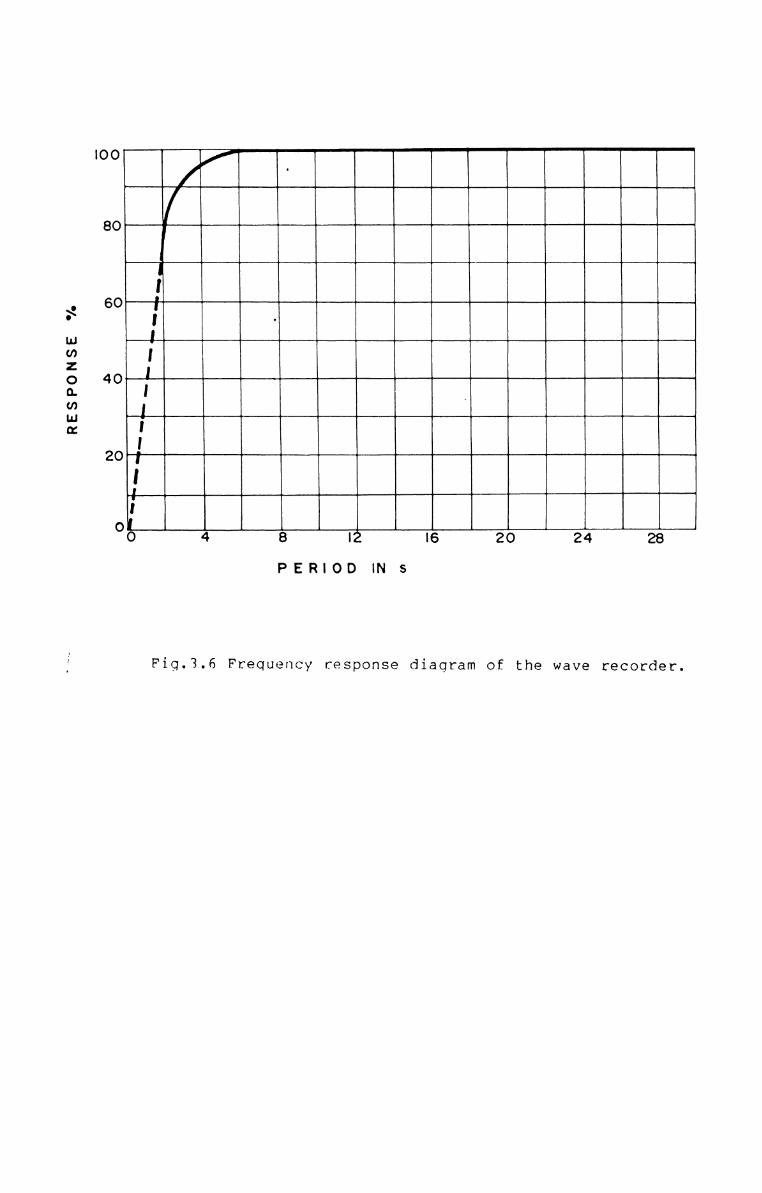
IOO

flk

RESPONSE

80

60

T

40

20

O ‘W: -0-. -4-.­ 24I6 204 8 IF’EF?|OI) IN S

Fig.3.6 Frequency response diagram of the wave recorder.

It is found that the response is more than 95% for waves ofperiod greater than 3 seconds and it is nearly 100% forwaves of period 5 seconds and more.

3.3. RECORDING PROCEDURE AND SCREENING OF RECORDS

The recordings were carried out for 30 min. at every3 hrs except during the periods of interruptions due topower failure, instrumental problems or servicing of thesystem. The predominant wave direction at the recordingpoint was also noted at the site using a Brunton Compass.

From the available records, those with the followingdefects or limitations are discarded:

- a drift in the mean zero-line due to instrumentalproblems;

— breaks in the records due to power failure, cablefault, instrumental problems, etc.;

- noise due to power fluctuations, vibration of thetransducer due to slackening of the installation; and

- near-straight-line records during very calm seas,particularly during the periods of mud banks.

All other records are considered for analysis.

3.4. PRELIMINARY ANALYSIS (TUCKER-DRAPER METHOD)

A reliable estimate of wave climate statistics can beobtained from the analysis of wave records collected

59

systematically over a sufficiently long period with a sampleof one observation per day (Thompson and Harris, 1972; Baba,

1983; etc.). The records collected during a four yearperiod (1980-1984), sampled am: one record per day, isselected for a preliminary analysis. This analysis iscarried out using the Tucker-Draper method (Draper, 1967;Silvester, 1974), which is regarded as the simplest of all.

In this method a portion of the record having a lengthof 720 s without any disturbance is selected for theanalysis. The Mean Water Line (MWL) is drawn by fixing itwith the eye. The heights of the highest and the secondhighest crests, A and B respectively, are measured from theMWL. Similarly the depths of the lowest and the secondlowest troughs C and D are measured. The number of zero­

crossings (NZ) and the number of crests (N are alsoC)

counted. Ewwmw these values the ciifferent statisticalparameters are estimated as detailed below.

amplitudeThe root mean square wave height (a ) can be computedFITIS

from the following equations:

Zarms/H1 1/(2lnNz)1/2 [l+(0.289/lnNZ)-(0.247/lnNz2)].....(3.1)

Zarms/H2 1/(2lnNz)1/2 [1-(O.211/lnNz)-(0.103/lnNz2)].....(3.2)

60

where H1 = A+C and H2 = B+D. As per theory, the results from

H1 and H2 should be essentially the same. ‘The statisticalerrors involved in this procedure are of the same order asaveraging the highest l/3 waves in the record forsignificant wave height, HS (Silvester, 1974). In thisstudy arms is determined using Eq.3.l. The spectral widthparameter (ew) is computed from

= .1 _ ooooo(3o3)This parameter helps to assess a more accurate proportion of

H1/10, HS and H. The ratio of these parameters to arms aregiven in the form of tables and nomograms in Silvester(1974).

The average zero-crossing period (T2) is given by

T2 = 720/NZ s .....(3.4)In order to compensate for the attenuation of pressure

with depth, correction is applied to the height parametersderived from this analysis using the following relation:

H = nHPcosh (2TTh/L)/cosh [(2TTh/L)(1-z/h)] .....(3.5)

where H and Hp are the corrected and un-corrected heightsand n is the instrument factor, L is the wave length corres­

ponding to T2, h is the water depth and z is the depth atwhich the transducer is installed.

61

Values ranging from 1.0 11) 1.5 have been assigned tothe instrument factor by various researchers (Homma et al.,,l966; Bergan et al., 1968; Cizlak and Kowalzki, 1969; Kurianand Baba, 1986; etc.). The value (M? 1.25 suggested byDattatri (1973) is used in the present analysis.

3.5. WAVE CLIMATE AT ALLEPPEY

The wave climate at this location is influenced by thesouthwest monsoon as is the case at any other location alongthe west coast of India. Following the suggestions of Thomasand Baba (1983) the data is grouped into two seasons ­‘rough season’ from May to October and ‘fair season‘ fromNovember to April.

3.5.1. Wave Height

The percentage exceedance of Hst and Hma for the twox

seasons are presented in Fig.3.7a. From the different perce­ntages of exceedance it is seen that the wave intensityduring the rough season is double of that-during the otherseason. When 25, 50 and 75 percent of Hst exceed 1.40, 0.95and 0.62 m respectively during the rough season, it exceedonly 0.70, 0.52 and 0.42 m respectively during the fairseason. Similar trend is shown by Hmax also. During therough season the above percentages of Hma exceed 1.90, 1.35X

and 0.85 m respectively and during the fair season they

62

exceed 0.95, 0.72 and 0.58 m. The maximum wave height obser­

ved during the rough season is 3.8 m and that during thefair season is 2.0 m. Similarly, the maximum value of Hstduring the rough and fair seasons are 3.0 and 1.4 m respec­tively. Eventhough the wave activity is maximum during the

month of June, the formation of the mud-bank brings in afew-weeks-long calm sea towards the end of the month.

3.5.2. Zero-Crossing Period

The zero-crossing periods ranged from 6 to 21 s withthe prominent periods falling in the range 7-15 s. Thefrequency, in percentage, for the two seasons are presentedin Fig.3.7b. During the rough season the waves are bettersorted and are of comparatively shorter periods, the mostfrequent being 8-9 s, which contribute to 31%» During the

other season waves with periods 9-ll s dominate and thiscontribute to 46% of the distribution.

3.5.3. Wave Direction

Though the wave direction range from 200-3200 withrespect to north, the majority of waves were confined to asmall range of 230-2650. The percentage occurrence of dire­ction of wave approach is presented in Fig.3.7c. The wavesare more parallel to the coastline during the rough season.The dominant direction during this season 1M5 245-2500 and

63

PERCENTAGE OCCUR R ENCE

(C)

PE RCE NTAGE EXCEEMNCE

--ROUGH~mFmR

31

F5 3 I I

--_..'—..————----—-1

_-__-..---_-_—J

C Y“'4

PERCENTAGE OCCURRENCE

6

VI 200 2|0 2207230 240 250 260 270 200 290 300 _3IO 32‘0WAVE HEIGHT(m) omgcnou ('94)

Ld). 35 r'135 <5’ ~ F——-ROUGH : 'II30v '7 —+- ROUGH 30 """ -‘"9 { :-—-- FAIR § } E25... - kg 25” : IAr‘? 3 r-——’--‘I Ir -120- u 20- I I° " —j' : :|5- 3 l5- ' 1S "4 IT 5 .|O-- 7-" __ 8 IO» F-——-1 *--f }+-—--J ._+ E5- 5 ~ __d. _ | __J "*05 3 no 214 :5 I8 20 0 0:5 05 OJ’ 03 092 L0

ZERO-CROS&N§ PERmD<s) Ga

Fig.3.? Wave climate at Alleppey during fair and rough season:H ('<8?’-‘ “”

percentage exceedance of wave heights, Hst andapd frequency dlstribution of zero-crossing periodd1rect1on (c) and spectral w1dth parameter (d)

this contribute to about one-fifth of the total of theseason. During this season 50% waves arrive from the direc­tion 245-260° and 83% from 235-265°. During the fair seasonthe waves are more southerly and about one-fifth of themarrive from the direction 235-240°. Waves from 230-2450contribute to 44% and that from 230-2550 contribute to 61%

during this season.

3.5.4. The Spectral Width

The spectral width parameter (e for both the seasonsW)

are presented in Fig.4.7.d as percentage occurrence. Thevalues range from 0.5 to 1.0 during both the seasons.However, the average value is less during the rough season.During this season 70% of the values fall in the range 0.6­0.8 and 90% in the range 0.6-0.9. During the fair seasonabout 60% of the values are in the range 0.8-0.9 and 90% inthe range 0.7-0.9.

3.5.5. Persistence of Waves and Calm

Persistence diagrams serve as a ready reference todetermine the number of times a range of wave conditions (ator above in the case of ‘persistence of waves‘ and at orbelow in the case of ‘persistence of calm‘) persist for atleast for a given length of time. The significant waveheights computed for three-hourly intervals during 1981 are

64

selected for the preparation of these diagrams. At times ofbreak in the data the wave condition prior to the interrup­tion is assumed for the elapsed time. This appears to bejustifiable since the nearshore wave characteristics shownear-stationary conditions for durations of the order of aday (Thompson and Harris, 1972; Kurian et a1., l985a,etc.).Persistence of waves and calm are presented for heightintervals of 0.25 m (Fig.3.8a-b). From the diagrams it canbe seen that high wave conditions persist for very shortdurations and low wave conditions persist for long durations

at this coast. For example, wave heights (Est) at or above2 m persisting for a day occurred on less than 20 occasionsonly during a year. It can be inferred easily from thesediagrams that if a study requires a minimum wave height of2.5 m persisting for 100 hrs, it cannot be conducted at this

location. Similarly, if wave heights (Hst) not more than 1 mprevailing for a minimum of 60 hrs is required for a parti­cular study, 95 such occasions are available during a year.

3.5.6. DISCUSSION ON THE WAVE CLIMATE

On an assessment of the distribution of the aboveparameters it can be seen that the waves during the roughseason exhibit certain characteristic features. They arewell sorted and arrive from the same generating area, asevidenced from the distribution of periods, directions and

65

NUMBER OF OCCURRENCES

F

NUMBER OF OCCURRENCES

5.

in­

(a)H.lN METRES

\\\ \\ \ I‘ \.‘ ‘\ \\ \ I\ \\‘ \xA A 44AAAAl A A A LL- 1 LA A A A AAAAloo 23468.07. 2 3463,02 sews s4sqo4

DURATION IN HOURS

0|oe

n_nn METRES

u

2 {Jo4 ".\_\ \‘2 ‘\‘ \\\ ‘ \I A .A1 . .4 - . L 1 L_ ‘o 2 3 4 6 0 u 2 3 4 6 8 2 2'": 4 5 a 3 2 3 4 6 e .I0 no IO no .0

DURAUON IN HOURS

ig.3.8. Persistence of (a) waves and(b) calm at Alleppey.

spectral width. The lower periods are indicative of a not­far-away origin of these waves. Evidently these are gene­rated under the influence of the south-west monsoon winds.

From the monthly wind speed summary for the Arabian Sea andNorthwest Indian Ocean (Boisvert, 1966) it is seen that from

May the winds get intensified, the dominant direction beingsouth-west. The intensification continues through June, Julyand August and the entire Arabian Sea and the North-westernIndian Ocean become the wave generating area. Wind speeds of,the order of 28 knots and more are reported all over thisregion. These winds prevail till September and the directionis reversed to northeast by November and continues tillMarch, April and October being the transition periods.During the fair season the waves are poorly sorted as wavesgenerated at different areas arrive at this coast. Thelarger period waves during this season associated withsmaller heights and lesser frequencies of cmcurrence indi­cate that these waves are generated at great distances andhave undergone different transformation processes like wave­wave anui wave-current interactions, shoaling, refraction,diffraction, etc. Incidently, the prevailing wind in theArabian Sea and the North-eastern Indian Ocean during thisseason has low velocities and north-easterly direction,leading to the generation of waves which also contribute tothe wave climate.

66

3 . 6 . DETAILED ANALYSIS

3.6.1. Selection of Records

The wave climate characteristics are found to vary onlyslightly from year to year during the examined 4 yearperiod. Hence, the wave records collected during a one yearperiod is selected for the detailed analysis of spectral andprobabilistic characteristics. Records collected during 1981are selected, as maximum number of records, with lessernumber of disruptions, are available during this year. Thus287 records, at the rate of one record per day (correspon­ding to 1200 Hrs), are used for the detailed analysis.

Since the coastal erosion is during the southwestmonsoon, a more intensive study of the wave characteristicsduring this season is also warranted. Hence, an additional30 three-hourly records collected for one month from mid-Mayare also utilised for this study.

3.6.2. Spectral Analysis

Two procedures are generally used to estimate the wavespectrum. One is using the data to estimate the covariancefunction first and then to compute the cosine Fouriertransform of the covariance function numerically, in turn tocompute the raw spectrum (Blackman and Tukey, 1958). Theother uses the Fast Fourier Transform (FFT) computer

67

algorithm (Cooley and Tukey, 1965) to get the raw spectrumdirectly from the data. The basic principle of FFT lies insplitting the given time series into two half-series, whichis performed many times during the process of computing thefourier transform. This involves lesser number of arithmetic

operations compared tun the covariance method, therebyleading to a large reduction in computation time. Both theprocedures give the same results except that the covariancemethod applies an intrinsic smoothing to the spectrum. Fromthe viewpoint of simplicity, computational speed andpreservation of information, the FFT method is pmeferable.The FFT method is applied here to compute the wave spectrum.

The stability and accuracy of the spectral estimatesdepend on many parameters such as the record length,sampling interval, spectral window used, high/low frequencycut off, etc. (Goda, 1974; Harris, 1974; Baba et al., 1986;;Kurian, 1987; etc.).

3.6.2.1. Digitization and processing

The records are digitized manually at 1 s interval, foraccuracy and simplicity in digitization, since each cm ofthe chart paper, on which the waves were recorded, isdivided into 6 divisions and the recordings were done on thechart running at a speed of 5 cm/s. In a few cases the

68

digitization is done at 1.2 s interval, since each cm of thechart paper is divided into 5 divisions in those cases. Forthe computation of spectral densities, 512 data points eachare utilized. This is sufficient to obtain a reasonablystable spectrum (Baba et al., 1986).

Usually the time series digitized at equal timeinterval is subjected to a trend removal procedure beforethe spectral analysis. Even in the absence of any trend ofsignificance, as the recording system used zhi the presentstudy removes the trends, the raw data is subjected to alinear trend removal, which makes the arithmetic mean of the

process zero.

3.6.2.2. Spectral window

In order to minimize the distortions in any desiredaspect of the'spectrum, spectral windows are applied.Eventhough the spectral windows are many, the most commonly

used ones are the ‘hanning’ and the ‘hamming' windows.Though the highest side lobe for the hamming spectral windowis about one-thind of the height of tflma highest side lobefor the hanning window, the heights cflf the side lobes forthe latter fall off more rapidly than for the former (Wilsonet al., 1974). The hanning window 1h; selected in thepresent study. The hanning window function for a digitizedtime series of N points is defined as:

69

Wi = 0.5 [l+cos 21T/N (i-(N+l)/2)] .....(3.6)

As a consequence of the application of this window all thespectral estimates have to be scaled by the constant factor

8fl70.375 and this is incorporated in the computer programme.F“

3.6.2.3. Pressure attenuation

The pressure spectrum thus computed is subjected topressure attenuation correction to obtain the surfacespectrum using the standard relation (Harris, 1972; Black,1978; etc.), which is given as

s<£) = [cosh (2TYh/L)/cosh um h/L)(l-z/h)]]2Sp(f)....(3.7)

Grace (1978) modified this relation by incorporating anempirical correlation factor, n(f), based on wave tankmeasurements. Since the use of this factor is not yet firmlysubstantiated and may introduce some uncertainty in thespectral data, as observed by Knowles (1982), it is notincluded in the present analysis.

3.6.2.4. Spectral parameters

In accordance with the frequency response of therecorder and the maximum wave period possible in thisregion, the low and high frequency cut off are fixed at 0.04and 0.33 Hz respectively in the computation of moments and

70

other spectral parameters. The different spectral parameterscomputed are:

(i) nth moment of the spectrum

mn = _f£”s(f)d£ .....(3.8)(ii) significant wave height

ass = 4(mO)1/2 .....(3.9)(iii) zero-crossing period

TmO’2 = (mo/m2)1/2 .....<3.1o)(iv) mean wave periodooooo(3oll)(V) mean crest period

1/2Tm2’4 = ooooo(3o].2)(vi) spectral band width parameters

es = (1-m22/mOm4)1/2 .....(3.13>= (momz/m12-l)1/2 .....(3.14)

1% = (1 - mlz/mOm2)1/2 .....(3.15)(vii) spectral peakedness parameter

Q = 2/mO2‘ffS2(f)df .....(3.l6)P

and (viii) slope of the high frequency side of the spectrum

S(f)oC £‘m ; fm < f < 1.8fm .....(3.17)3.6.2.5. Smoothing

The wave spectrum obtained from the FFT method ofanalysis exhibits details much more than that required for

71

applications like graphical presentation and comparison withtheories. The irrelevant details are usually suppressed byapplying a smoothing function. The smoothing depends on the

type of smoothing applied and the number of spectral linesused. In the comparison of the observed spectrum with theo­retical ones a well-smoothed spectrum would be much usefulsince the theories are developed for single-peaked spectrumonly. However, in the present case the prominent peaks areretained to get a clear picture of the actual wave condi­tions prevailing in the region of study. A weighted avera­ging method of smoothing (Ou, 1977) is applied here toobtain 33 bands with 16 degrees of freedom, without the low/high frequency cut off, for comparison with the theoreticalmodels and for graphical presentation.

3.6.3. Wave-by-Wave Analysis

In wave-by-wave analysis the zero-crossing method isgenerally accepted as a standard procedure. In this method,the MWL fixed by the eye, is drawn for the selected lengthof the record. The individual wave heights and periods canbe measured by following two procedures, zero-up-crossing orzero-down-crossing methods. In the zero-up-crossing method,the points where the wave record crosses the MWL in anupward direction is marked and a wave is defined between twosuccessive zero-up-crossings. The height of the wave is the

72

difference in elevation between the highest crest and thelowest trough between the two up-crossings and its period isthe time interval between these two crossings. Similarly, inthe zero-down-crossing method a wave is defined as the onebetween the tan) successive zero-down-crossings. The heightand period of the wave is defined as in zero-up-crossingmethod. Individual wave heights and periods may differ inthese two methods and hence the estimate of the maximum wave

height in a record also may be different. However, in acomparative study of the two methods of analysis, nosignificant influence of the method is observed in theheight statistics particularly H and Egg and in therms

probability density distribution (Dattatri, 1985).

In the present investigation, the zero-up-crossingmethod of analysis is carried out for the study of thedistributions of wave heights and periods. The heights andperiods of individual waves are derived from the digitizeddata using a computer algorithm (Varkey and Gopinathan,1984). This programme identifies the individual wave by thezero—up-crossings and measures the maxima and minima and the

corresponding periods. The exact wave height is calculatedfrom the interpolated crest and trough values usingStirling's formula (Scarborough, 1966). Necessarymodifications are made in the above algorithm to incorporate

73

the correction for pressure attenuation as applicable to thelocation of study and the recording system employed.

In accordance with the frequency response of therecording system (Fig.3.6) waves with period less than 3 sare scanned out. The higher non-linear effect due to theexponential increase of the pressure attenuation correctionfactor (Eq.3.5) in the lower periods are also eliminated bythis scanning. However, this removes the lower period tailof the probability density distributions. Since the densityand energy in this range are not significant this does notaffect the probabilistic characteristics. The different

H 'fi,Theight and period parameters (H T and TS),max’ sw' c’ zspectral width (ew), steepness, individual and jointdistributions of heights and periods are determined from theremaining individual waves.

74

CHAPTER 4

OBSERVED WAVE SPECTRAL AND STATISTICAL CHARACTERISTICS

The observed wave spectra, the spectrally obtainedparameters and the statistical characteristics obtained fromthe ‘wave-by-wave zero-up-crossing analysis are presented.Characteristics of the different parameters during rough andcalm sea conditions are identified. Relations between thevarious parameters are also examined.

4.1. OBSERVED SPECTRA

Typical examples of the observed spectra are depictedin Fig.4.1. The spectra are generally multi-peaked. Out ofthe 317 spectra examined, 286 exhibited multi-peakedness.

being the frequency correspon­The peak period (Tp= 1/fm, fmding to the maximum energy density, known as the peak fre­quency) and the period corresponding to the major secondarypeak are examined. The major secondary peak periods rangedfrom 2-16 s with energy density varying from 0.01-2.74 m2s.The secondary peaks are generally on the lower period sideof the main peak. When the average and standard deviationof peak periods are 11.2 and 2.5 s, thomeof the major secon­dary peak period are 6.4 and 3.1 s respectively.

Various reasons are put forward for the existence ofmultiple peaks in shallow waters. Multiple peaks can be due

75

HII: 0.50 m. Tp : 8.0 I HI‘: 0.50 m. Tp : 12.8 I0-l6 0-51 02m008‘ I1 .-1 O" ‘A je .‘O O r ‘Y r v f W T O O Y 1 T 1 1 T IQ0 01 oz 03 0+ 90 on O2 03 04A H15: 1.49 m. Tp : 8.5 I HI5: 1.51 m. Tp -. 12.8 IU)

(\)E 5-04V . [.5 1> ~ ‘~.1.) -I.,..4 ‘ .4U) .. _ ­C '0 4Q) 05‘ -1'C 4 :r—-4 -4 _ -J(O O 5 ‘L: " 44.: . 4U .Q) Y 7 T Y Y Y r 0 O 1 T r 1 f I V3* oo» on oz 04 0+ on 0! O2 03 0*H151 2-7-7 m. Tp : 8.5 I HI5: 2.48 m. Tp : 11.0 I

4-0

'1

4-0"-1

2-0-1-1 2(‘oJ0.0 V V 2 ‘f 5 Y T 000 Y 5 Y Y V f fon as o¢ as 04- 00 0” 04 03 “*­

Frequency (Hz)

Fig.4.1 Typical examples of observed spectra.

to the co-existence of swells and wind waves. Peaks athigher harmonics of the peak frequency can occur due to thenon-linear effects in the shallow waters. When a single­peaked spectrum propagates to the shallow waters, increasingfraction of the energy will be shifted to the higher harmo­nics of the dominant frequency (f mainly due to wavem)

breaking. As a result of this the spectral peak at twice the

peak peak frequency (2fm) can be higher than the peak at fm(Sawaragi and Iwata, 1976; Dattatri, 1978). Another situa­tion in which multiple peaks are generated is when the wavescross a submarine bar. When the crest level of the bar isclose to the water level, much of the energy is shifted tothe higher harmonics and multiple peaks with almost equalenergies are developed (Thompson, 1974; Dattatri, 1987).This is a special case of the non-linear interaction of seabottom on the passing waves. '

In the present case, the secondary peaks are notgenerated by submarine bars since no such topographicalfeatures are present in the shallow waters off this coast(Kurian et al., 19855» The secondary peak periods do notshow any dependence on the peak periods. In the plot of themajor secondary peak periods against T (Fig.4.2) wideP

scatter is observed. Very few values fall along the second

harmonic of the peak frequency (2fm-:1/(Tp/2)). Most of thevalues are lower than Tp/2 with a few in the range Tp-Tp/2

76

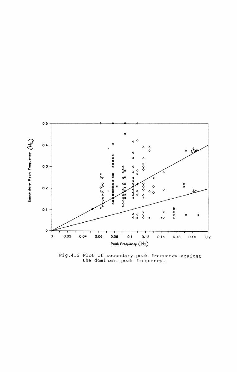
Secondary Peak Fnqucncy

0,5 % <3‘ <‘r -GO

O O 00°‘ " o oO O OO0 ‘O 0O0 O0.25 - 0 0 O

0 OO00 3 o0 O3 00.2 -1 Q Q90 g oO 03 3 °

O0 99'” o 0 o0 0 O O O 00 o 0 o 00 o

0 “ I I I I I I I I I W I I I I I I0 0.02 0.04 0.06 0.08 0.1 0.12 0.14 0.16 0.18

Peak Frequency <

Fig.4.2 Plot of secondary peak frequency againstthe dominant peak frequency.

0.2

and some even higher than Tp. The ratio of peak period tomajor secondary peak period ranged from 0.4 to 8 with anaverage of 2.1 and a standard deviation of 1 s. Among the286 spectra with multiple peaks only 37 have the secondarypeaks at the second harmonic of the peak frequency. The

spectra for which secondary peaks are at Tp/2 are thosehaving comparatively higher peak periods. The 1%) in thesecases range from 9.14-19.2 s with a mean of 12.46 and astandard deviation of 1.84 s. In the study of averagespectra for US coastal waters, Thompson (1980) observed the

major secondary peaks at Tp/2 for waves of peak periodshigher than 10 s, especially for large wave heights.However, in the present case no dependence on wave height isobserved (figure not presented). Hence, in most of thecases the secondary peaks observed may be due to the co­existence of swell and sea waves in this region.

4.2. OBSERVED SPECTRAL PARAMETERS

The different spectral parameters like significantwave height, peak period, slope of the high frequency side,spectral width parameters and spectral peakedness of theobserved spectra are examined. The distribution of theseparameters during the complete year as well as during per­iods of characteristic wave properties, like rough and fairwave conditions, are discussed in the following sections.

77

4.2.1. Significant Wave Heights

The significant wave heights (HSS), computed withEq.(3.9), ranged from 0.13-2.48 m during the period ofstudy, with an average of 0.78 and a standard deviation of0.52 m. However, it may be noted that the recordsrepresenting very calm periods are not included in theanalysis (see Sec.3.3), otherwise the minimum would have

been much lower. From the temporal variation of HSS(Fig.4.3) it can be seen that the wave height start toincrease from the month of May and reaches the maximum value

by mid-June. Then it decreases and attains lowest values bythe first quarter of October. The low heights persist forthe rest of the year. Intermittent calm periods are foundto occur from the last quarter of June consequent to theformation of mudbanks.

As seen above, the higher waves occur during May­September. The maximum Hss observed during this season is2.48 m and the average for the season is 1.15 with astandard deviation of 0.52 m. The months of October-April is

characterised by the low waves. The maximum HSS observedduring this season is only 0.97 m and the average is 0.44 mwith a standard deviation of 0.18. Barring the calms duringthe mudbank periods, the lowest wave heights are cmservedduring October-December.

78

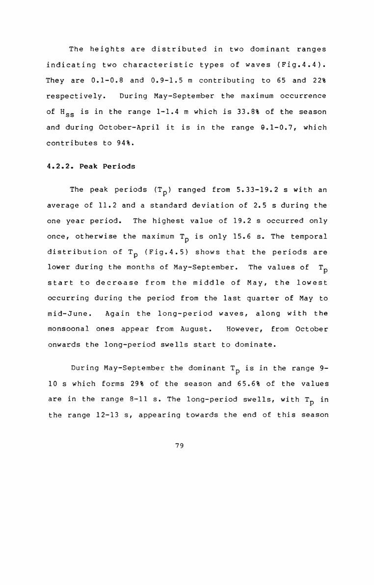
The heights are distributed in two dominant rangesindicating two characteristic types of waves (Fig.4.4).They are 0.1-0.8 and 0.9-1.5 m contributimg to 65 and 22%respectively; During May-September the maximum occurrence

of Hss is in the range 1-1.4 m which is 33.8% of the seasonand during October-April it is in the range 0.1-0.7, whichcontributes to 94%.

4.2.2. Peak Periods

The peak periods (Tp) ranged from 5.33-19.2 s with anaverage of 11.2 and a standard deviation of 2.5 s during theone year period. The highest value of 19.2 s occurred onlyonce, otherwise the maximum T is only 15.6 s. The temporalP

distribution of Tp (Fig.4.5) shows that the periods arelower during the months of May-September. The values of Tpstart to decrease from the middle of May, the lowestoccurring during the period from the last quarter of May tomid-June. Again the long-period waves, along with themonsoonal ones appear from August. However, from Octoberonwards the long-period swells start to dominate.

During May-September the dominant Tp is in the range 9­10 s which forms 29% of the season and 65.6% of the values

are in the range 8-11 s. The long-period swells, with T inP

the range 12-13 s, appearing towards the end of this season

79

v in

,mD tnTm afimn m#9 FL+..U_..wWO Q

Ma w4 .1u 1 sWU r5 F.I. 0

IV

I|J%|lU n. A O.1

7.... t.U)F. r olsmi . 5

Y D

oltY dhgH 1.1H mm

i

O

a D..eT m vear7A Tw

EM 3as .+3 A9F g

«.1

r% .1i... F

_ . _ _ « . _ . _ _ 4.

5 A .‘ 2 3 .» 4 at 1 3 .o 4 .‘ o

. O O. O. .

7 ,7//// /./////////////////////A7 /,V A.7//%r4 2 0 8 G 4 2 0 8 6 4 2 O

2 2 2 1 1 1 1. 1

7%%%%@m.////////­

21

Significant Wave Height (m)

Fig.4.4 Frequency distribution of significante height (HSS).wav

contribute to 17.9% of the distribution. The average Tp du­ring this season is 10.2 s with a standard deviation of 2.2.

During October-April the dominant Tp is in the range12-13 s which contributes to 54.2% during this season. Waves

with two other characteristic periods with T at 10-11 s andP

15-16 s also exist during these months. They contribute to

16.3% and 14.5% respectively. The average Tp during thisperiod is 12.1 with a standard deviation of 2.4 s.

The major secondary peak period values do not show any

characteristic variation with season. They range from 2-16 sduring both the seasons (May-September and October-April)with an average of 6.4 s. However, the variation is lessduring October-April, as indicated by the standard devia­tions (3.7 during May-September and 2.4 during October­April). These can be the contribution from the locallygenerated waves. The contribution of these waves to thetotal energy of the spectrum are very little when comparedto that by the swells.

‘The frequency distribution of Tp (Fig.4.6) shows thatwaves with three different characteristic periods dominate

in this region. Among these, Tp in the range 12-13 sdominate with 36.9% during the one year period followed bythose in the range 9-11 s which contributes 33.4%. It canbe noted from the figure that when the distribution is

80

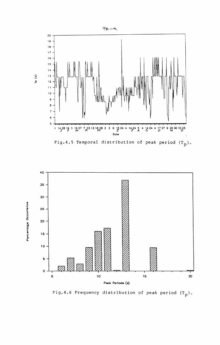
Port: ontogc Oc currcnce

V0 (5) 55M M ” ME: 7'1 1r4J2rz3:'g;:'§1;7 ;A;3:3;%2; ; 3 I L ;

Fig.4.5 Temporal distribution of peak period (Tp).%3o~ Egg%

20-— IéM %//ad %M % %V /fl% 7% /o,%A,%%é.¢t z ,Ui It’3..3:

Fig.4.6 Frequency distribution of peak period (Tp).

continuous in the lower period ranges, it is discrete atnarrow intervals at 12-13 s and 15-16 s. Dominance of the

three typical Tp ranges (8-11, 12-13 and 15-16 s) is indica­tive of the arrival of waves of different characteristicsfrom different generating areas. Following the discussionin Ch.3 (Sec.3.5) it may be inferred that during May-Octoberthe Arabian sea is the generating area for the waves arri­ving at this coast. During October-April the major contri­bution is from the long-travelled swells generated at twoother far-off locations, one farther than the other.

4.2.3. Slope of the High Frequency Side of the Spectrum

The slope of the high frequency side of the spectrumcalculated using Eq.(3.l6) sometimes gives erroneous results

due to the presence of secondary peaks within the range fm­l.8fm. The cases where the major secondary peaks fall inthis range are excludedfrmnthe following discussion.However, other peaks, though not significant, may also aff­ect the slope values. Since the number of observationswithout any peak in the range fm-1.8fm are very few, therecords with such minor peaks (in the above range) are notexcluded. The slope values thus computed range from 0.22­4.76 with an average of 2.57 and a standard deviation of0.97. There is considerable variation in slope during allthe periods (Fig.4.7). However, a slight decrease in slope

81

is observed during May-September. The values start decrea­sing from May and the lowest are observed in June. It againincreases with the retreat of this season. The averagevalues for May-September and October-April are 2.32 and 2.72

with standard deviations of 0.85 and 1.01 respectively.

The values are almost normally distributed (Fdg.4.8)with the peak in the range 2.1-2.2. However, when they aresplit into the two seasons, the peak is shifted to the lowervalues during May-September and to higher values duringOctober-April (figures not presented). The maximum occurren­

ces during May-September and October-April are in the ranges2.00-2.25 and 3.00-3.25 respectively. Also, secondary peaksexist in the distributions in the ranges 2.50-2.75 and 3.50­3.75 during the above two seasons respectively.

It is to be noted that in shallow waters the slope ofthe high frequency side of the spectrum is always lesscompared to the equilibrium range value of wave spectralform in deep water conditions. In the shallow waters, theslope of the spectrum are reported to be lower by many rese­archers (see Sec.2.3) and values as low as 1.6 are reported.

In deep water, during the process of wave growth, non­linear wave-wave interaction/white-capping/breaking play animportant role. Due to these processes some of the energy

82

Port ontagc Oc curnnco

Stope

as­

‘-1

1s—

3.4

as­

2­

L5­

1-:

05 "mmmmmqmmmwmmmmmwmmmwmmwmmmmmmwmmwmmwmmmwmmmmmq

1 j2aF «kin Ax: L3 1%. g_ a‘ gs 50 m g, 5 025Date

Fig.4.? T 1 distrib ‘on of slope theh' equency si of the spe um.

26

24-122- ?2o~ //. ::)‘°“"‘‘°‘e~ /yygg‘W21 7% / /%/0 /////// 1271T r I ' T ' I ' I r T’O 1 2 3 4 6Six:

Fig.4.8 Ftequency distribution of slop f thehigh frequency side of the spe um.

from the higher frequencies are transferred to the lowerfrequencies. Frequencies higher than fm loses energy whilefm and frequencies lower than it gain energy as a result ofthe non-linear effects (Vincent, 1982). This results in anincrease in the slope of the high frequency side of thespectrum. But, the shallow water waves are almost unrelatedto the local wind conditions and hence the predominant wavesobserved in the shallow waters are generated elsewhere andpropagated to the area of observation, after undergoing thedifferent transformation processes like shoaling, refrac­tion, diffraction, wave-wave/wave-current interactions, etc.The wave-wave interaction is comparatively insignificantduring the propagation of waves outside the generating areaunless it crosses over other fetches. It is the frictionalattenuation that is important during the wave propagation inshallow waters and the energy loss will be more for waveswith higher energies (Kurian, 1987). Consequently the slopeof the high frequency side of the spectrum decreases signi­ficantly. It may be inferred from the above that the wavestravelling over gently sloping bottom in shallow watersexhibit spectra with lesser slopes, when the local wavegeneration is not considered.

The still lesser slope observed during the monsoonperiods may be due to the increased effect of frictionalattenuation as the waves are of higher energy during this

83

season. However, most of the present data contain multiplepeaks and hence the slope values computed with the presentdata cannot be used to check the dependence of the slope ofthe high frequency side of the spectrum on peak periods.

4.2.4. Spectral Width

The spectral width parameters presently in use are 8,1)and Lh(Eqs.3.l3-3.15). The temporal distribution of theseparameters computed from the wave spectrum are depicted inFig.4.9 (a-c). Almost identical distributions are observedfor these parameters. The values are comparatively lowerduring May-September. They start decreasing from May andreach the lowest value in June. With the withdrawal of this

season, high values are once again observed. The highestvalues are observed in October. The range and averagevalues of these parameters during both the seasons arepresented in Table 4.1. This again shows that May-Septemberis characterised by spectra with lower widths as evidencedby the low average values and the lesser scatter indicatedby the standard deviation. The lower values observed duringthis season may be due to the predominance of wavesgenerated by the monsoonal winds which have almost identicalcharacteristics and the lesser significance of the lowswells arriving from far-away locations. On the contrary,the higher values during October-April are the effect of the

84

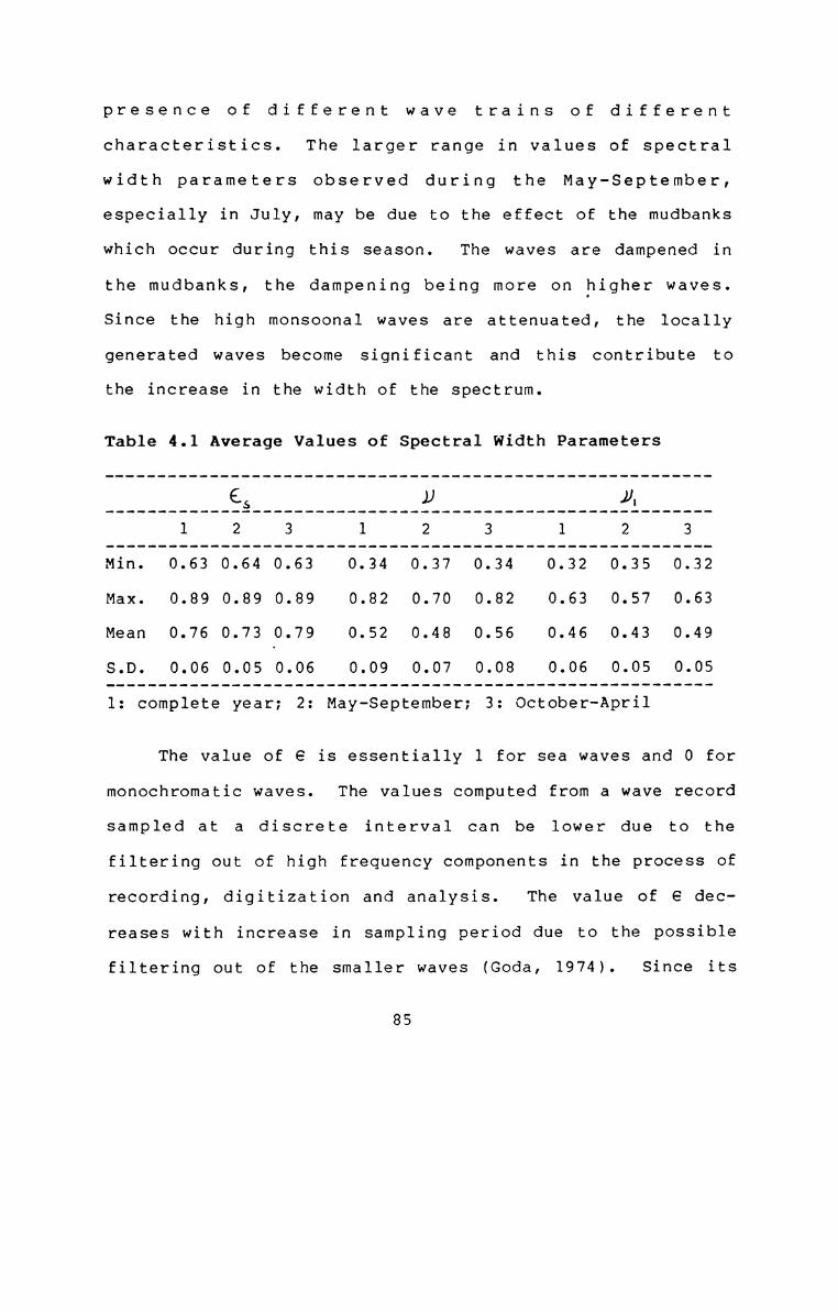
presence of different wave trains of differentcharacteristics. The larger range in values of spectralwidth parameters observed during the May-September,especially in July, may be due to the effect of the mudbankswhich occur during this season. The waves are dampened in

the mudbanks, the dampening being more on higher waves.Since the high monsoonal waves are attenuated, the locallygenerated waves become significant and this contribute tothe increase in the width of the spectrum.

Table 4.1 Average Values of Spectral Width Parameters

Min. 0.63 0.64 0.63 0.34 0.37 0.34 0.32 0.35 0.32Max. 0.89 0.89 0.89 0.82 0.70 0.82 0.63 0.57 0.63Mean 0.76 0.73 0.79 0.52 0.48 0.56 0.46 0.43 0.49S.D. 0.06 0.05 0.06 0.09 0.07 0.08 0.06 0.05 0.051: complete year; 2: May-September; 3: October-April

The value of G is essentially 1 for sea waves and 0 formonochromatic waves. The values computed from a wave record

sampled at a discrete interval can be lower due to thefiltering out of high frequency components in the process ofrecording, digitization and analysis. The value of G dec­reases with increase in sampling period due to the possiblefiltering out of the smaller waves (Goda, 1974). Since its

85

value is 1.0 for sea waves it cannot represent the shape orbandwidth of sea wave spectrum. However, in the shallowwaters where the swells dominate this parameter can beuseful in determining the sea state, since the sea wavescontribute to an increase in its value.

The frequency distribution of es (Fig.4.10a) shows thatthe maximum occurrence is in the range 0.75-0.8 (28.1%)followed by nearly equal frequency (25.2%) in the rangeimmediately preceeding this, when the complete year is con­sidered. when the data is divided into the above 2 seasons,it is seen that the lower values correspond to May-Septemberand the higher to October-April. During May-September themaximum occurrence is in the range CL7-0.75, which consti­tutes 35.8% of the season, and 93.4% are in the range 0.65­0.80. During October-April the maximum number of observa­tions are in the range 0.80-0.85 with a. 36.7% occurrence.However, 81.9% fall in the range 0.70-0.85.

The frequency distribution of L’shows two major maximaindicating the existence of two different characteristicwaves (Fig.4.l0b). The maximum occurrence is in the range0.50-0.55 followed by 0.45-0.50, the former being 29% andthe latter 28.4% during the year. The naximum occurrenceswith the above ranges correspond to the two seasons. DuringMay-September the values in the range 0.45-0.50 constitutes

86

Spectral width (65)

Spectral width ( 1) )

0.9

0.85

0.8

0.7

0.65

0.6

0.55

0.9

0.5 -J

0.7 ­

0.6 -1

0.5 -1

0.3

-4

(a)

T' V ‘I I *1 V71142519 31527 7 23131328 2 3 51524 4-14245M A M :r 3' A3' F

T‘ 7 I W fiYY Y —I fi‘lT"T‘fi—r r‘1’“f‘T TN41424 41727 9 203010255 O N D

r-'r—* ‘I

Date

(b)

I 1 1 f I 1 T‘ Y 1

1142819 31627 7 23131828 2 3 61524 413243‘TFMA1 F Y I’ 1 I

M[Date

Y I 7 ‘T Y I Y “Y '7 ‘I f I T I T W41424 41727 9 203010250 H D\

Fig.4.9 Temporal distribution of spectral widthparameters:(a) G (bu) ; (c) 11,.S7

Port: cntogo Oc curra nco

(H)

11‘ W “A

1142819 31627 7 23131828 2 3 51524 41424 4124417279 301025I’ F M A r1 3 3 X 3 c) $3 9Dots

”iQ.4.9 continued.

24%

22­2011e~

16­

14~

12~

10—

8-4

442-4

<\ * \\\\\\\\\\\\\\\V \ \\\\\\\Vx\\\\\\\\\\\\\\\\“1\\\X\\\\\\\\‘«ts0.5 0,7Spectral Width Porcnwcter

Fig.4.1O Frequency distribution of spectral widthparameters: (a) es; (b);) ; (c)14,

to about 41% of the season. During October-April the valuesare slightly higher and the maximum occurrence is in therange 0.50-0.55 followed by 0.55-0.60 which are 38% and 29%

respectively of this season.

The distribution of.U1 is similar to that ofy(Fig.4.lOc). When the complete year is taken, the maximumnumber of values fall in tflme range 0.5-0.6 (38.8%) with anearly equal frequency for the range immediately preceedingthis (36.9%). As in the case of 1/ when the data is dividedinto the two seasons it is seen that the lower values belongto May-September and the higher values to October-April.The maximum occurrence during May-September is in the range

0.4-0.5 which is 58.3% of the season and that duringOctober-April is in the range 0.5-0.6 which forms 52.4% ofthe values during the season.

4.2.5. Spectral Peakedness

The spectral peakedness parameter, Q (Eq.3.l6) variedP

from values as low as 1.6 to as high as 11.4 with an averageof 3.5 and a standard deviation of 1.5» No characteristicvariation with month or season is observed in its temporaldistribution (Fig.4.ll). However, the occurrence of highervalues are less during May-September. The seasonal averagesfor May-September and October-April are 3.2 and 3.9 withstandard deviations of 1.2 Emmi 1.6 respectively. ‘The fre­

87

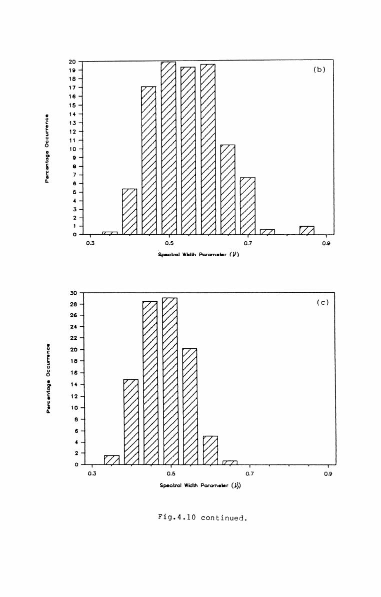
(b)

m,mV///// /T W

//////%////x/ /////////////////% /Y///////////////////////M

/ /fl/ /1%

/ //////V////////// x7/M///1

Qndnflwuh

0 9 8 7 6 5 4 3 2 1 0 9 8 7 6 5 4 3 2 10

2111111‘:

(c)

7//,7///////////// /,/ ////////////////////z7///////////,0 8 6 ‘ 2 O 8 5 4 2 O 8 6 4 20

3 2 2 2 2 2 1 1 1 «I1

M“/ ////////////fl////////4/j M

Spectral Width Porcrncier

Fig.4.1O continu

quency distribution (Fig.4.l2) shows that the maximum number

of occurrence is in the range 2.5-3.0 which constitutes24.9% with 74.1% in the range 2.0-4.0. The season-wisedistribution also shows that the maximum occurrence are in

the range 2.5-3.0 during both the seasons, with 29.8% duringMay-September and 20.5% during October-Aprils During May­

September 84.8% are in the range 2.0-4.0 and during October­April 64.5% are in this range.

The values of spectral peakedness Qp is dependent onthe cut-off frequency, presence of secondary peaks andfrequency resolution. Using the theoretical JONSWAP spectra

Rye (1979) has shown that Qp is little affected by the ratioof the Nyquist frequency to time peak frequency. But, thepresence of relatively large secondary peaks causes to

decrease the value of Qp. With an increase in frequencyresolution, which decreases the effective degrees of freedom(d.f.), the spectrum gets sharpened, as a result of which

the value of (*3 is increased significantly. when thefrequency resolution is increased from 0.0156 to 0.00098 Hz

(decrease of effective d.f. from 84 to 4.6), the value of Qpis raised from 2.7 to 8.4 (Goda, 1983). As a solution Rye(1982), based on his judgement of analysed data andsimulation studies of wave profiles with JONSWAP spectrum,recommended the number of d.f. of about 16. Hence, a

88

Pen: ontoge Oc currnnco

Spectun Peokedness (00)

11-‘

10­

9-4

8-4

7-4

5­5* 4I4-1 ; I3. g

2-4

1__.'_r._.1‘—‘1'—'fi—1,—*(.r1r—‘r.yw1'1rrfi"T"T1T‘Y1v1 1:}281'9:31'6427 7g31:sP1’ia2a 2 3 511524 4 13424§‘414s2441Z)27 9 23301035

Date

Fig.4.11 Temporal distribution of spectralpeakedness parameter (Qp).

-45

4o— //4'

30-420­15- :§? Egg1o— Egg éfij////5-4 J/i/'70, ,17.Z1//,//Pl71F'71. V71. ,r-no 5 10

Spectnol Pookedncan (op)

Fig.4.12 Frequency distribution of spectralpeakedness parameter (Qp).

recalculation of Qp values is made using the smoothedspectra with 16 d.f. When smoothed, the values are reducedconsiderably. They range from 0.77-2.44 with an average anda standard deviation of 1.39 and 0.30. These values do notshow any decrease during May-September, rather a slight

increase is observed during the peak monsoon months (June­July). The values are slightly lower during August-October.Hence the average values for the seasoms do not show muchdifference. The averages for the above seasons are 1.40 and1.39 with standard deviations of 0.29 and 0.30 respectively.This is contrary to the observation with higher frequency

resolution. From these results it may be inferred that Qpis not dependent on the seasonal properties of waves. A

plot of the Qp values with and without smoothing (effectived.f. 16 and 2) is given in Fig.4.l3. No correlation isobserved between these values. This may be due to theinfluence of secondary peaks. When higher resolution isprovided the secondary peaks can be strong at differentfrequencies. when smoothing is done some of the secondarypeaks are suppressed considerably depending upon the

spectral estimates in the nearby frequencies. That is, Qpcan be taken as a wave pmoperty only when secondary peaksare negligible. Goda (1983) also observed that it is notadvisable to calculate the spectral peakedness parameterbased (N1 spectra vdifli large fluctuations. ‘R1 the shallow

89

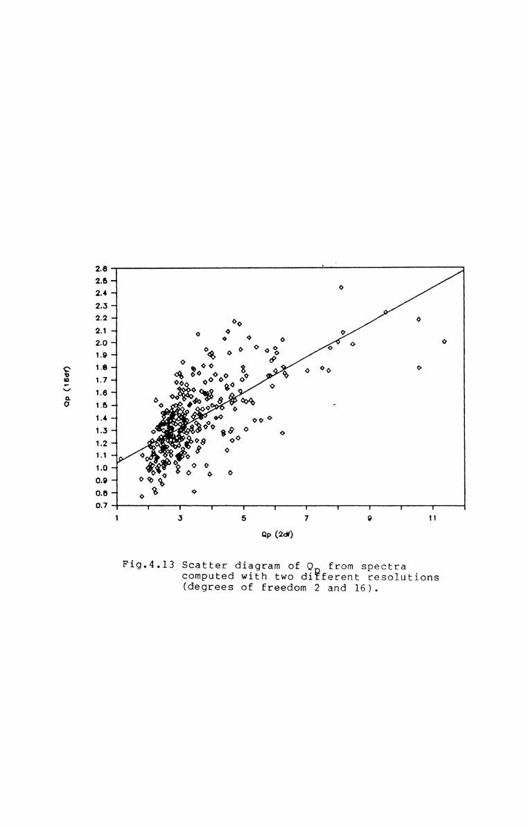
Qp (16:10

2.82.6 -J

O2.4 -.12.3 -<2.2 - 00 o2.1 -4 0 oo 9 0 O2.0 -1 o1.9 _. Q 0 &01.8 -* 0 Q °° 3 0 0° 0<3 0° 0'0 o %1.7 -1 0° 90 09.0 0 O1.8 -1 ‘)&w16 - 00 O“ 8 (30% ». O 01.3‘ 0 9 O o1.2 J "8 °°1.1 -J 0 &o 8 OO1.0 Q? 0 O0.9 -1 9 QQ3 —. O 3 O0-7 I I I I I I* T I r II .3 5 7 9 H

Op (2c§)

Fig.4.l3 Scatter diagram of Q from spectracomputed with two di¥ferent resolutions(degrees of freedom 2 and 16).

water conditions multi-peakedness is a common phenomenon due

to various reasons as discussed in Sec.4.l. In general, Qpcannot be taken as a criterion for drawing conclusionsregarding the characteristics of waves in shallow watersunless there is a single-peaked spectrum.

4.3. AVERAGE SPECTRA

Individual shallow water wave spectra may be quiteirregular and change substantially with tine. In order toidentify typical spectra for a particular condition it isdesirable to condense the individual spectra into a moreconcise form. Presently there is no satisfactory techniquein use for isolating and summarising general characteristicsof field spectra. (hue of the usual methods is ix) computespectral statistics, which are based on the moments of thespectrum. Hoffman (1974) grouped the spectra according to

H53 and computed the mean and standard deviation of thespectral densities in each band. Some other researchers

made the grouping according to H58 and Tp values(Gospodnetic and Miles, 1974; Thompson, 1980; etc.). Thisapproach seems to be more reliable since the averagespectrum for a specific height-period range providesinformation on the various distinct characteristics of theparticular wave condition. However, the averaging has to bedone according to the specific purpose for which it is

90

required. For example, if the wave condition for aparticular season is required it is desirable to compute theaverage spectrum for that season irrespective of the waveheight/period values and compute the statistical parametersfrom it. On the other hand, for characterising the spectrumfor its shape or to compare it with a theory, it isdesirable to compute the average spectra according to somespecified characteristics such as height or period. In thisstudy the monthly average spectra is computed to exploreinformation (N1 the monthly average wave characteristics.Similarly, the average spectra for height and periodintervals of 0.25 m and 1 s are computed to examine thespectral shape and to compare with different models.

4.3.1. Monthly Average Spectra

The monthly average spectra are presented in Fig.4.14.The spectra are puedominantly single-peaked; no nmjorsecondary peaks are observed. However, secondary peaks with

lesser energy generally occur during October-April. Thesecondary peak becomes most clear in April and from Mayonwards it starts to disappear. Again it makes itsappearance in October and persists during the rest of theyear. When the secondary peak energy is of considerablemagnitude (about 25-35%), they are at twice the peakfrequency. During the other occasions, they are around this

91

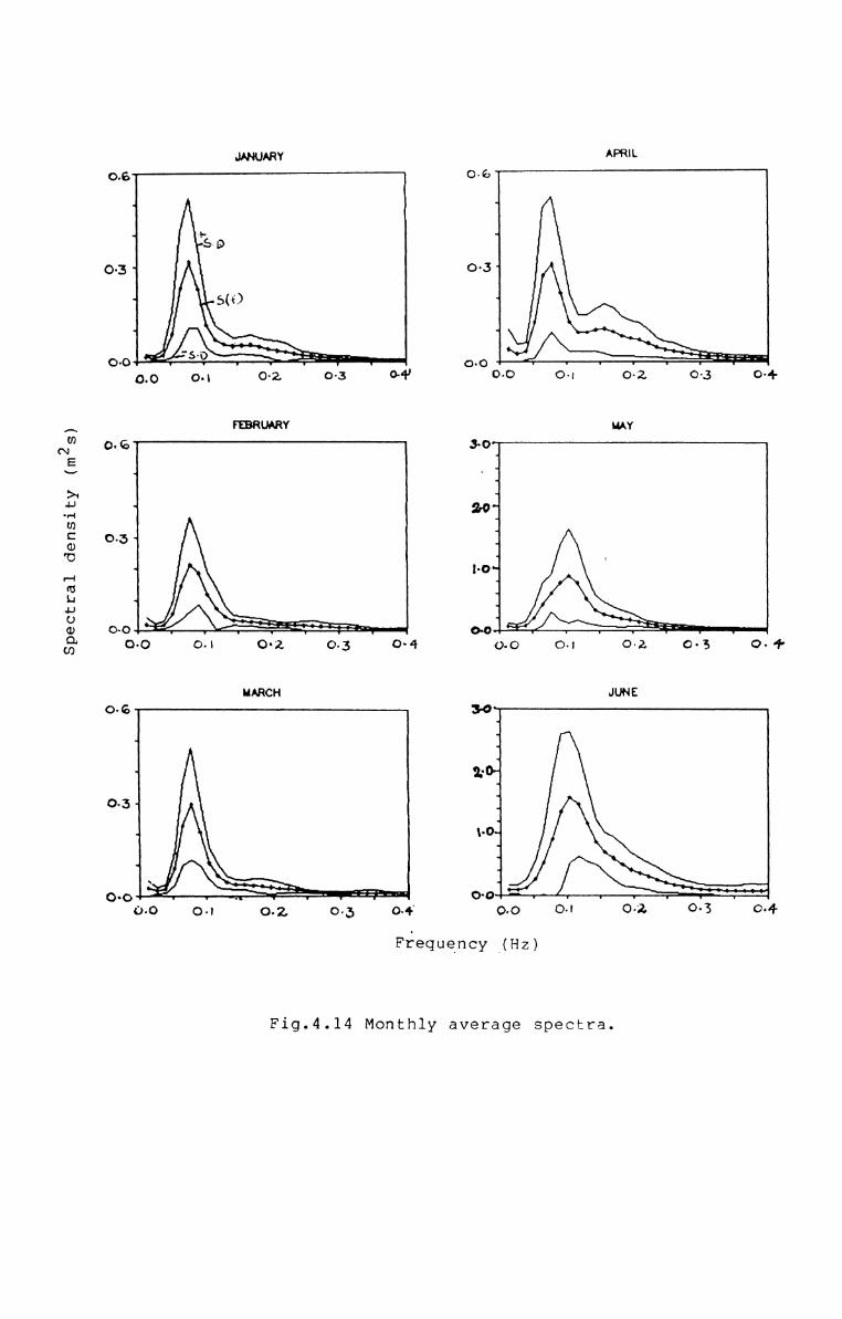
JANUARY APR“

A rmaumv wwU)N O» G 3-0 4E -1§/ * 4S. -J_H * zojm -1E.‘w d'0 -4

youI-1 -4G .LI4-’ ‘IO '1G) 0-03 0.0

MARCH JUNE(>6 30*J 1+1 2.0-+03 1. vol

000‘ - _ °‘G 1‘ V A f v W0.0 0.1 0.2, 0.5 o.4' Q0 0.! 0-2. 0-3 O-4­Ffequency (Hz)

Fig.4.l4 Monthly average spectra.

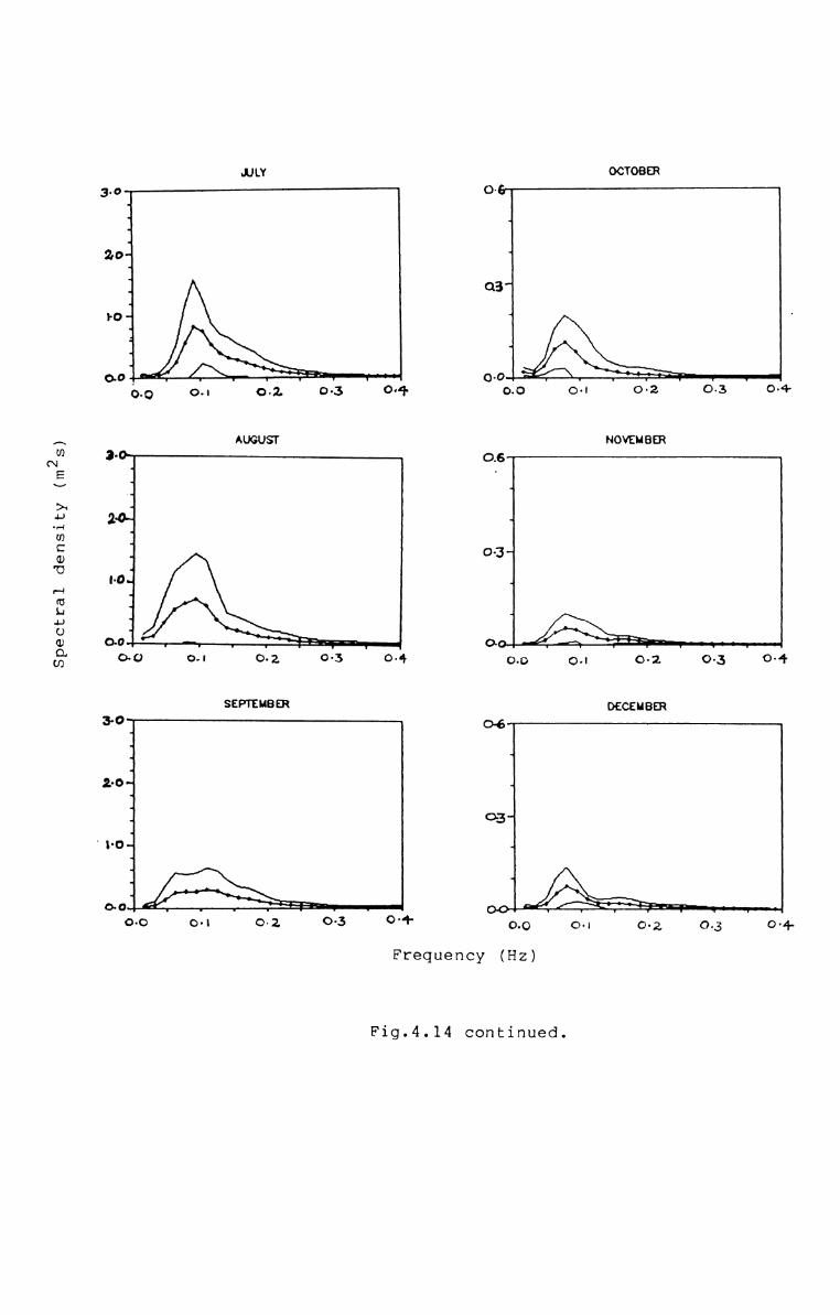
AJLY

‘I’0

.L1;n.nlLL11

9o

AUGUST

Spectral density (m2s)

smwmmun3-0

1

2.0....JJ

4

J

8'0­

1

1oo­o&> ow cwz <>3 <W+

OCTOBER

0-4}

03‘-4

o‘0_!_ T 1o.o 0-! 0-2 0-3 0-4­NOVEMBER

0.6

031-4

* ; A ,'0.0 0.1 0-2 0'3 0-4­DECEMBER

0-6

'4

-+

Ofifi

'100a + ‘ '7 ‘0:0 0 l 0'2 0 3 0'4‘Frequency (Hz)

Fig.4.14 continued.

value, and are of lesser energy density, the maximum energydensity of these being only 17% of the peak energy density.

The spectral parameters computed from the averagespectra are presented in Table 4.2. The energy is highduring May-September with the highest in June and the lowestin November. Among tflmz lower energies present duringOctober-April, the post-monsoon (October-December) iscomparatively calmer. The average HS during May-SeptemberS

is 1.16 with a standard deviation of 0.26 m and that duringOctober-April is 0.47 with a standard deviation of 0.14 m.These average values agree with the averages computed withthe individual values for both the seasons (1.15 m duringMay-September and 0.44 m during October-April).

Tp values are lower during May-September, as observedin the distribution of individual values, and they vary from9.1 to 11.0 s with an average of 10.0 and a standard devia­tion of 0.70 s. During October-April the peak period isconstant at 12.8 s. The variation of spectral width parame­

ters (€S,;}and H.) during both the seasons are identical tothat discussed in the previous sections. Hence a detaileddiscussion is not presented here.

From the above discussions it can be seen that thewaves during May-September and October-April exhibitcharacteristic properties of heights, periods and spectral

92

Table 4.2 Spectral Parameters from Monthly Average Spectra

May 1.12 9.6 0.90 1.34 2.74 0.79 0.52 0.46Jun 1.64 9.6 1.58 1.27 2.11 0.75 0.52 0.46Jul 1.06 11.0 0.82 1.40 1.96 0.76 0.50 0.44Aug 1.13 10.7 0.74 1.06 2.26 0.86 0.69 0.57

widths. May-September is characterised by high wavesassociated with comparatively shorter periods and spectralwidths. During October-April low waves with comparativelyhigher periods and spectral widths persist at this location.Hence, the former may be classified as ‘rough season‘ andthe latter as ‘fair season‘.

93

4.3.2. Average Spectra at Height-Period Ranges

Mean spectra are computed for significant wave heightand peak period intervals of 0.25 m and l s. Those spectracorresponding to the lower energy conditions and lower peakperiods exhibit multiple peaks. The major secondary peaksobserved in such cases are mainly in the range 15-16 s. Thedominance of this period is an indication of the presence oflong travelled swells in this region. However, as seen inthe previous section, the presence of these waves are notnoticeable at higher energy conditions, as the energy con­tent of these waves are very low compared to the monsoonalones. The presence of secondary peaks observed at the lowerperiods in the spectra having very low and very high ener­gies may be due to the lesser number of records availablefor averaging. When the number of spectra available foraveraging is more, the secondary peaks may be smoothed out.

The spectral parameters of these average spectra showwide variation compared to the average of the spectralparameters computed for the height ranges (see Sec.4.4).One of the reasons for this variability may be the lessernumber of spectra available for averaging in certain rangeslike the lower as well as the higher heights and periods.Hence the cases, where average could not be taken due toavailability of only one spectrum in that particular range,

94

are not included for the following discussions. Anotherreason for the higher variability of the parameters may bethe presence of multiple peaks in some ranges. The slope ofthe average spectra range from 1.58 to 3.43 with a mean of

2.41 and a standard deviation of 0.45. The Op values rangefrom 1.02 to 1.57 with an average of 1.3 and a standard

deviation of 0.14. Since slope and Qp are more susceptibleto errors with the presence of secondary peaks, the caseswhere major secondary peaks are present are also notconsidered for this calculation. Relations between theparameters derived from these average spectra are examinedin the following section along with the discussion on therelation between the parameters derived from individualspectra and their averages at specified height intervals.

4.4. RELATION BETWEEN THE SPECTRAL PARAMETERS

The correlation between the spectral parameters arecomputed and the coefficients are presented in Table 4.3.On a comparison of the above parameters significantdependence is shown by the spectral width parameters only.

The spectral width parameters €s,fl and U, show goodcorrelation between each other. A plot of es and‘u,againstyis presented in Fig.4.1S..M exhibits very good positivelinear dependence onl/and a correlation coefficient as highas 0.93 is observed (Table 4.3).

95

By definition 1} and Lfl are functions CHE Oth, 1st and2nd moments of the spectrum. From Eqs.(3.14) and (3.15) itcan be seen that

14 = L/2/(1+1/2) .....(4.1)Hence a better correlation can always be expected.Moreover, either.fl or L4 can be used, since they areinterchangeable through Eq.(4.l). As the properties andvariations of these parameters are identical, only one ofthem need to be considered for practical applications.

Table 4.3 Correlation Between the Spectral Parameters

op -0.10 ~0.31 1.00 0.33 0.08 0.04 0.14es -0.40 0.19 0.33 1.00 0.77 0.76 0.732J -0.46 0.13 0.08 0.77 1 00 0.93 0.9114 -0.44 0.11 0.04 0.76 0.93 1 00 0.69Tp -0.32 -0.06 0.14 0.73 0.71 0 69 1.00

8 also shows good positive correlation withfl(Fig.4.1S) and a correlation coefficient of 0.77 is obtai­ned. The linear regression fit of G8 with 1/ is given by

GS = 0.535)} + 0.48 .....(4.2)96

es by definition is a function of 0th, 2nd and 4th momentsof the spectrum. Hence it gives a different conceptcompared to J’ and.U,. However, the usefulness of theseparameters .hs questioned knr some researchers. Goda (1974)

suggests that €S vary with sampling interval and hence itcannot be regarded as a good estimate of the spectral shape.

He presents Qp as an alternative to es, 1/ and L5 to deter­mine the shape of the spectrum. Rye (1976) examined thevariations of these parameters with the cut-off frequency.

His results show that €S,)J and H, vary with the cut-offfrequency, the maximum variation being in the values of es,

and Qp is non-dependent on the cut-off frequency. Hence healso recommended Qp to characterise the spectral shape in­stead of €S,fl or.N. . However, Q is dependent on theP

frequency resolution (Goda, 1983). Also, the pmesence cisecondary peaks, which is 21 characteristic feature (N5 theshallow water wave spectra, affects its values. In thepresent study values of Op do not show any characteristicvariation with the wave conditions (with heights, periods or

seasons). However, €S,.U and 1% exhibit such a characteris­tic dependence (Sec.4.2.4). Since the frequency resolutionand digitization interval are kept constant in the present

analysis, the values of Qp are not affected by the frequencyresolution and the variations in €S,.fl and LG are indepen­dent of the sampling. Hence, the characteristics observed

97

in €s,.fl and .U, can be attributed to the wave characteris­

tics. Thus, it is reasonable to conclude that Qp cannot beregarded as 51 good shape parameter for shallow water wave

spectra . On the other hand, though es, y cm: 14 cannot beregarded as good estimators of the spectral shape, they canbe considered for a qualitative determination of thepresence of different sea and swell wave components.

The other parameters that show mutual dependence are

the spectral width parameters and T? €s,1/and .V, exhibitP.

good correlation with T with coefficients of the order ofP!

0.69 and more. The values of these parameters are found toincrease with T eventhough with some scatter in theirplplots (Fig.4.l6a-c). The best fit of these parametersobtained from linear regression analysis are

es = O.17STp + 0.564 .....(4.3)11: 0.246Tp+O.248 ......<4.4),U,= 0.016Tp + 0.278 .....(4.5)

As a result of the dependence of the spectral widthparameters on T the variation of T €S,)/and.bGwith otherP’ P’parameters are almost identical. These parameters decreasewith increase in energy. They decrease until HSS takes avalue of about 1.4 m and then onwards (for the higher wave

98

Spectral Math: (19, and 9

Spectral math, 9

0.9

0.8 -1

0.7 --4

0.6 -*

0.5 ­

0.4 -1

0.3

00

0.3W I I T0.5 0.7

Spectral Width ()1)

A )5 o 5%

Q9

Fig.4.lS Relation between spectral width parameters.

0.9

0.8 -1

0.3

000

O9

0

OOWO‘

3 10 12 14Peak Period (Tp)

20

Fig.4.16 Relation between peak period and spectral widthparameters :(a) u ; (b))4 ; (c) 6 SO

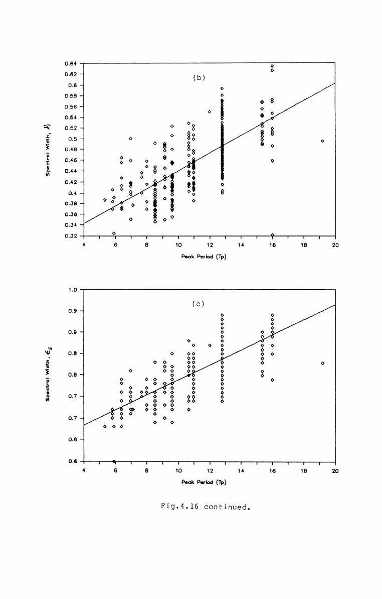
18181410 12Peak Period (Tp)

Fig.4.l6 continued.

02

o 0

Ya

rm

80 arm 00 0

000 000000000

I4

008.-I3 1 mm’. 0000000000 0000000000

/I\

0 rflw 0

b M .m

my 0

,.m

1|

I8

1

0000:6 ooo

____afi1«+qq4a_~4 4~J_fidfi«

L.26864n45884248642 O 9 9 8 8 7 7 6 6££0.5.5.6.5.O.A4.4.4.0.JJJ3 1. 0 0. 0 0. 0. 0. 0. Q

00 0000 0000 0000

‘R .523 _obuoaw ....w .533 _n.auoam

energy conditions) they remain almost stationary. The highenergy waves occur during May-September and enxa the waves

generated in the Arabian Sea due to the strong monsoonalwinds (see Ch.3). They retain their characteristics (as seenin the previous sections) and hence the lower values of the

above parameters prevail for the larger wave heights withoutappreciable change. Since the higher period waves are thosegenerated at farther places compared to the monsoonal waves,it is quite possible that the shorter period waves generatedat nearby places also arrive along with the tdgher periodwaves, resulting in higher width of the spectrum in theshallow water. But for the high energy monsoonal waves theyhave the generating area at comparatively nearer places andhence possibility of occurrence of other short period wavesgenerated at still lesser distances are less resulting innarrower spectra with lower peak periods.

In addition to the examination of individual values ofspectral parameters, their averages at height intervals of0.25 m are also examined. The dependence of the variousparameters discussed above are exhibited more clearly by theaverage values. An interesting result observed in thiscomparison is the correlation of the slope of the spectrumto the energy. The average slope values decrease systemati­

cally with increase in mo (Fig.4.l7). The best fit isrepresented by the relation

99

- 6;4zc=35«

slope = 2.651 - 4.l4mO .....(4.6)Similarly, the relations obtained between the spectral widthparameters and peak periods are also more clearly indicated

with the average values. The plots of es andJ4againstyare presented in F%g.4.18. The following relation isobtained against Eq.(4.2).

es = + ooooo(4o7)Plots of the spectral width parameters against T areP

presented in Fig.4.l9. The best fit lines corresponding toEqs.(4.3-4.5) are obtained as

es - 0.026Tp + 0.462 .....(4.8).N - 0.044Tp + 0.029 ......<4.9)L4: 0.029Tp + 0.133 .....(4.1o)

Whereas considerable scatter is observed when theindividual values are considered, the average values exhibitvery little scatter. Hence, the relations depicted from theaverage values can be considered as representative of therelationship between the parameters.

The relations observed above, between the average ofthe spectral parameters in specified height ranges, arefound to follow qualitatively in the case of the spectral

100

Sbpe

Spectral Width Param stars

3.02.9 "‘2.82.7

2.6 -'\I2.52.4 -42.5 -I2.2 -‘2.1 -‘2.0 ‘I

la L

-A i c-L j -0 i fi C‘ i I I O O O . . . ­

b

L1 9

0.85

I I I I I I I0.1 0.2 0.3E""‘9Y (mo)

Fig.4.l7 Relation between slope and energyof the average spectra.

0.4

0.8 fi

0.75 "i

0.7 ‘J

0.65 "

0.6 "

0.56 -4

n64

0.45 -I

0.4 -I

0.360.40

Fig.4.18 Relation between the average spectral width

I I I I I I I I I I I I I I I I I0.42 0.44 0.46 0.48 0.50 0.62 0.54 0.66 0.58

Spectral Width Ponorncter, 1)+y, o 55parameters in specific height intervals.

I

0.60

parameters derived from the average spectra in the specifiedheight-period ranges also. The regression equationsobtained with these parameters are slightly different fromthe ones presented above. The standard errors of estimatesare less in the case of Eqs.(4.6-4.10) and hence they may beused for all practical purposes.

4.5. STATISTICAL PARAMETERS FROM WAVE-BY-WAVE ANALYSIS

The distributions cfif the different statistical heightand period parameters obtained from tflma wave-by-wave zero­

up-crossing analysis are discussed in this section.

4.5.1 Heights

The ranges, averages and standard deviations of themaximum wave height (fimax), significant wave height (Hsw)and average wave height (H) obtained from the wave-by-wave

(zero-up-crossing) analysis are presented in Table 4.4.Since the temporal and frequency distributions of the signi­

ficant wave height obtained from the spectral analysis (HSS)are already presented in Sec.4.2, the above distributions of

Hswaxe not presented here. Similarly, as Hma and E arex

related to the significant wave height, and a comparison ofthese are to be made in Sec.4.6, the distributions of theseparameters are also not presented here.

101

Table 4.4 Observed Height Parameters (Average)

1: complete year; 2: May-September; 3: October-April

H and H for the year as a wholeThe ranges of Hmax, SWand that during the months May—September are found tx> bethe same. The lower values during the months of intense wave

activity is the result of calms prevailed amidst the monsoondue to the formation of mudbanks. However, the averages arein agreement with the observation made in Sec.4.2.

4.5.2. Periods

The different wave period parameters obtained by thewave-by-wave zero-up-crossing analysis are presented inTable 4.5. The average periods (T2) are in the range 6.4­l3.7 s. The mean of T2 is 9.3 with a standard deviation of1.4 s during the year. The range of T2 during the rough andfair sea states are almost the same as that observed for thecomplete year. However, the range is slightly narrowerduring May-September. The mean of T2 during this season is

102

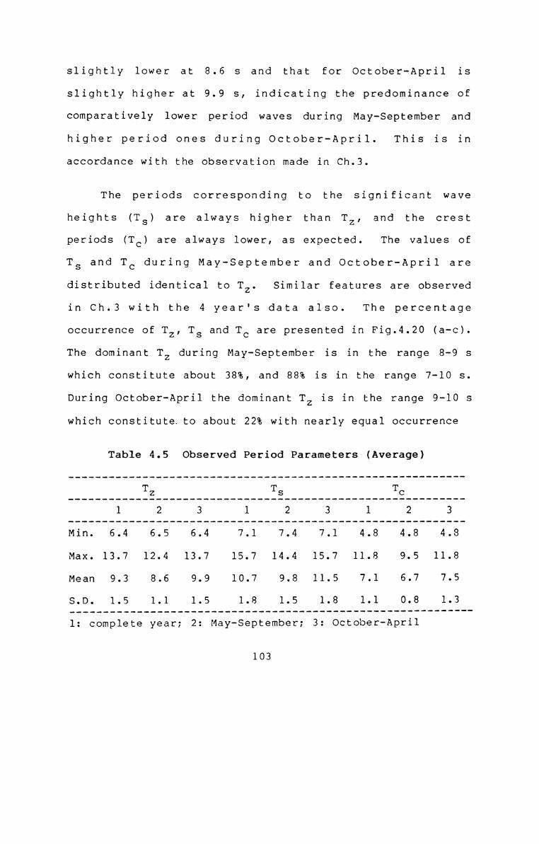
slightly lower at 8.6 s enui that for October-April isslightly higher at 9.9 s, indicating the predominance ofcomparatively lower" period waves during May-September’ and

higher period ones during October-April. This is inaccordance with the observation made in Ch.3.

The periods corresponding tn) the significant waveheights (T5) are always higher than T2, and the cmestperiods (TC) are always lower, as expected. The values ofTS and TC during May-September and October—Apri1 aredistributed identical to T2. Similar features are observedin Ch.3 with the 4 year's data also. The percentageoccurrence of T2, T8 and TC are presented in Fig.4.20 (a-c).The dominant Tz during May-September is in the range 8-9 swhich constitute about 38%, and 88% is in the range 7-10 s.

During October-April the dominant T2 is in the range 9-10 swhich constitute.to about 22% with nearly equal occurrence

Table 4.5 Observed Period Parameters (Average)

1: complete year; 2: May-September; 3: October-April

103

Spectral Width Porom ctnra

Pen: ontoge Occurrnnce

0.8

0.76 -1

Q71V#>#’~

0.65 -1

0.6 -1 .

0.66 ­

0.6 -1

0.45 -'1

a4 9 10 11 12 15Peak Period (Tp)+ V, o H A 63

Fig.4.19 Relation between average peak period‘ and spectral width parameters in

specific height intervals.60

(a)

50-1 ‘|i4o- I\E30 ‘“ E2~z1;~aV rW10-1 ‘/éR?0 A1, 1 4-1111 ma1 ‘ 1 * V ' 1 r4 6 8 10 12 14 16

c tFkww.T12:21 1.-or '°'1’::J nou§+«"" roar

Fig.4.2O Frequency distribution of period parametersfor rough season, fair season and whole year(a) Tc; (b) TZ; (c) TS.

40

(b)35­

30-‘

fl//I’.//”””’/II.//‘I’./’ ,

V‘_‘-~‘~.-~.---‘-~

26-*

20"1

16­00... OLLJU 00 32:. ouch

10-4

16_ 12 14Zero-croui Period. T1 (0)(SS? Rough Fair

10

E33 1)vw

(c)

_A /W//4///KW

7///K/////K/W/Kr

nwnnxdnflmnna

nW NM \N\\\\N\NN\\\N\\N\u

NR .N _W//////////4//Mrq a .1 q 4 _ fl . _ _ 4 _, q 1

08642o8642086420

32222211111

ouc Ptao 00 Iooaco Pin.

16141210

FairZ2] two! sgutfifimgmo (9)

Fig.4.2O continued.

in the next lower and higher ranges. About 80% of T2 valuesduring these months are in the range 8-12 s. Thedistribution of TS and TC are also identical to that of T2.However, during each season the dominant Ts values are indistinctly separate ranges. During May-September themaximum number of TS is in the range 8-10 s (56%) and duringOctober-April it is in the range 10-13 s (61%). Thetemporal distribution of periods are found to be identical

to that of Tp explained in Sec.4.2 and hence a discussion isnot presented here.

4.5.3 Spectral Width

The spectral width parameter ew varied from 0.33-0.94during the year with an average of 0.63 and a standarddeviation of 0.1. The values are slightly lower during May­September and are confined to a comparatively narrowerrange. During this season it vary from 0.39-0.85 and duringOctober-April it ii; hi the range 0.33-0.94. The averagesduring May-September and October-April are 0.62 and 0.64with standard deviations of 0.1 and 0.09, respectively. The

percentage cmcurrence cflf ew during May—September, October­April and the complete year are presented in Fig.4.21. The

dominant ew values during May-September and October-Aprilare in the ranges 0.6-0.65 and 0.65-0.7, respectively, bothconstituting about 24% of the respective seasons. The above

104

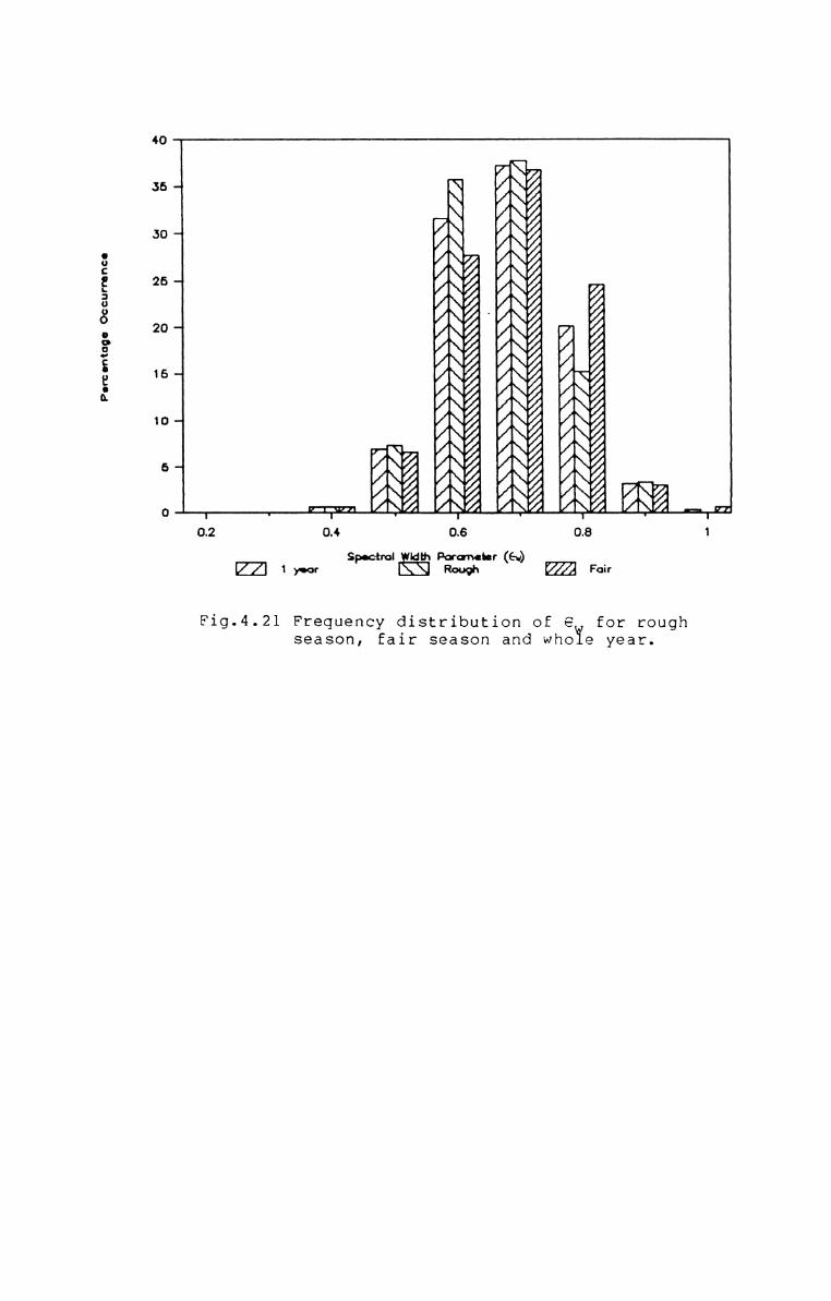
Porc ontoge Occurrenco

40

35­

.30‘

26­

20'­

15-1

10­0 ET 3I— ' fl ' * I * * * W * * ‘0.2 0.4 0.6 0.8Spectral ldlh PorcrnchrE Iysor Fair

Fig.4.21 Frequency distribution of e for roughseason, fair season and whoie year.

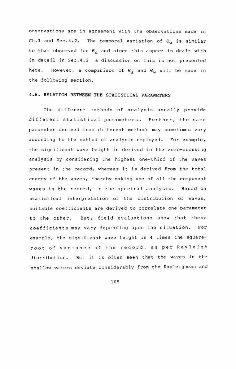
observations are in agreement with the observations made in

Ch.3 and Sec.4.2. The temporal variation of ew is similarto that observed for es and since this aspect is dealt within detail in Sec.4.2 a discussion on this is not presentedhere. However, a comparison of es and ew will be made inthe following section.

4.6. RELATION BETWEEN THE STATISTICAL PARAMETERS

The different methods of analysis usually providedifferent statistical parameters. Further, the sameparameter derived from different methods may sometimes vary

according to the method of analysis employed. For example,the significant wave height is derived in the zero-crossinganalysis by considering the highest one-third of the wavespresent in the record, whereas it is derived from the totalenergy of the waves, thereby making use of all the componentwaves in the record, in the spectral analysis. Based onstatistical interpretation of the distribution of waves,suitable coefficients are derived to correlate one parameterto the other. But, field evaluations show that thesecoefficients may vary depending upon the situation. Forexample, the significant wave height is 4 times the square­root of variance of the record, as per Rayleighdistribution. But it is often seen that the waves in theshallow waters deviate considerably from the Rayleighean and

105

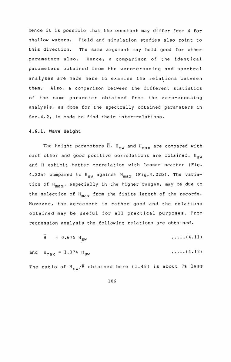
hence it is possible that the constant may differ from 4 forshallow waters. Field and simulation studies also point tothis direction. The same argument may hold good for otherparameters also. Hence, a comparison of the identicalparameters obtained from the zero-crossing and spectral

analyses are made here to examine the relations betweenthem. .Also, a comparison between the different statisticsof the same parameter obtained from tflma zero-crossinganalysis, as done for the spectrally obtained parameters inSec.4.2, is made to find their inter-relations.

4.6.1. Wave Height

The height parameters H, H and Hmax are compared withSW

each other and good positive correlations are obtained. Hswand H exhibit better correlation with lesser scatter (Fig.4.22a) compared to Hsw against H (Fig.4.22b). The varia­max

tion of H especially in the higher ranges, may be due tomax’

the selection of Hmax from the finite length of the records.However, the agreement is rather good and the relationsobtained may be useful for all practical purposes. Fromregression analysis the following relations are obtained.

E = 0.675 Hsw .....(4.11)and Hmax = 1.374 Hsw .....(4-12)The ratio of Hsw/H obtained here (1.48) is about 7% less

106

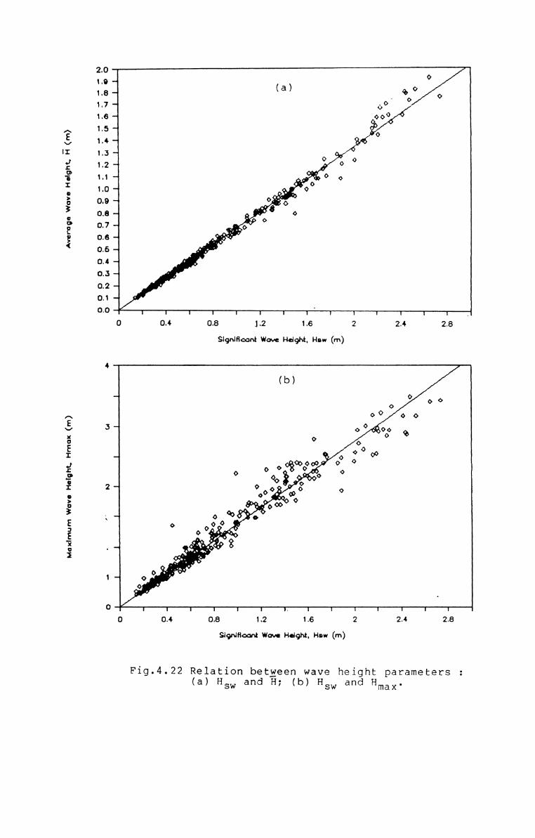
Average Wave Height, F: (m)

Maximum Wave Height, Hmox (m)

L

.aI.a_a.a-a.-0.0-auofg '-iou+uIo:~Imoo

1 1 J

‘o L

0.9 "0.8 -*

0.7 -1Q640.5 -4

0.4 -I0.3 -I0.2 ­0.1 -I0.0

0.4I

0.8I I I ' I I1.2 1.6 2

Significant Wave Height, Haw (m)

(b)

I I. I I I1.2 1.6 2sngnmoant Wave Height. Haw (m)

Fig.4.22 Relation betyeen wave height parameters(a) H

SW and H; (b) Hsw and H max’

than the theoretical value of 1.6 based on Rayleigh distri­bution. This may be due to the deviation of the wave heightdistribution from the Rayleighean in the shallow waters.

4.6.2. Wave Periods

The different wave period parameters'show varyingcorrelations with each other. The zero-crossing periods T2and the period of the significant wave (TS) show betterdependence with lesser scatter (Fig.4.23a). The crest period

(TC) also exhibit linear dependence, though with somescatter (Fig.4.23b). The plot of TC against TS (Fig.4.23c)show wider scatter. The average relation between theseparameters are obtained as

!-3 IIS 1.15 T2 .....(4.13)*-3 IIC 0.76 T: .....(4.14)

The period parameters T8, T2 and TC show wider scatter withthe period of maximum energy density (T ) obtained fromP

spectral analysis. On regression analysis the followingrelations are obtained between these parameters.

TS = 0.936 Tp .....(4.15)T2 = 0.81 Tp .....(4.16)T = 0.61 T .....(4.17)

Significant Period. To (3)

Crott Period, Tc (3)

1817 -4 (a)16 “ O15* o °oo o 0” 314 -‘ 0 O . . 8 80 0 "' O13— 0 %>°?° ° 0W _.. ogggo 00 08° 012-4 00 '4. 3 3.: O

90 O0 3300 9... . 3 3811a aw ' °.oO °3 o0 3 ‘:'-.10 . 6&0 %’..".o'. . O.0 *6"9 _‘ % .I.“_¢:-1 0 0‘...‘..-4-.: -C8 “‘ & 9; ..0° 0 O7 _I 0 00

6 "15 T I I I I I I f I5 7 9 11 13Z¢ro—-cnonnlng Period. T1 (9)12 iv v

(b)

10

3 I I I I I I 1 I5 7 9 11 13Zero—crona'r\g Period. 1': (9)

Fig.4.23 Relation between different period parameters(a) T2 and TS: (b) T2 and TC; (c) TS and TC.

15

The peak frequency (fm = 1/Tp) which is an input parameterin all the spectral models and in almost all practicalapplications can be obtained from these equations. However,usually the significant wave height (H and the period8)

corresponding to these waves (T are usually employed.S)

Eq.(4.l7) can be used to obtain fm from TS,~and from thepresent data the relation

fm = 1/1.07 Ts .....(4.l8)is obtained. Different values are suggested for the constantin Eq.(4.l8) by various researchers. The value is suggestedby Bretschneider (1977) as 1.057, by Mitsuyasu (1969) as1.06, by Goda as 1.08 and tmrihi (1977) as 1.13. The valueobtained zhi the present study :h3 closer txa the valuessuggested by majority of the researchers and hence Eq.(4.l8)

can be applied to obtain fm for this as well as for othercoasts with similar characteristics.

4.6.3. Spectral Width

A comparison between the spectral width parametersobtained from the spectral analysis is already presented inSec.4.4. A comparison of these parameters with thatobtained from zero-crossing analysis (e is presented here.W)

es and ew do not show much dependence between each other‘byshowing large scatter (Fig.4.24a). However, L/and.U1 are

108

Croat Period, Tc (3)

Spectral Width Pammetor

163 I I T T I T I6 8 10 12 14

SI-gtifloontP«¢riod, 159(9)

Fig.4.23 continued.0.0 '00 O Oo ooo O o o oo (3)o,e5- o o o o ooo co 4 o oo o o6 56 ® 0 C 0do 0 o 0 ca» o o0 0 0 060000 00 o o o0.8“ O 0 ¢ 000 O O O Oo o o co oo o 0$0 00000 $00 00oo oooo cm 000 coo oo 0O0 000 0 00 0000 o0.754 on o oo o oooooo o o 9 oo oooo coo oo ooo oo9990 C @009o o o co oooO6 0000 00 3 O 000,74 0 o o oooo o o coo oo o o oo oo oo ooo oo o o o o90 0000 00 <9 0 90.65-‘ 0 9 o oooo

0.64

0-55 I I ‘*1 I 1 I0.3 0.5 0.7 0.9Fig.4.24 Relation between spectral width parameters ­(a) G

W and ES;

Spectral Width Poranehr (6,)

(b) EW and H I (C) E

W and )1, .

found to be better correlated to ew (Fig.4.24b-c) thoughwith some scatter. The regression relations obtained forthese parameters are

.U 0.82 ew .....<4.19)1/ 0.72 ew .....(4.2o)

The poor dependence of es and SW may be attributed to theanalysis procedures used tun derive them. inn the zero­crossing analysis, the lowest waves, which do not cross the

MWL, are filtered off while theyaj-\eretained in the spectralanalysis. Hence, depending on the characteristics of thewave records (time series), the values computed with eachmethod may differ by varying extents. This applies to theparameters L’and.U1 also. But, es is a function of thehigher moments, thus is more influenced by the frequencies,

unlike L’or .L’I which are functions of the lower moments.This may be the reason for the comparatively betterdependence obtained forl/and JJ1 with ew.

4 . 7 . CONCLUSIONS

The multi-peakedness observed in more than 90% of thespectra obtained from this location is mainly due to the co­existence of different wave trains arriving this coast fromdifferent generating areas. The waves occurring during themonths cflf May-September exhibit distinct characteristics.

109

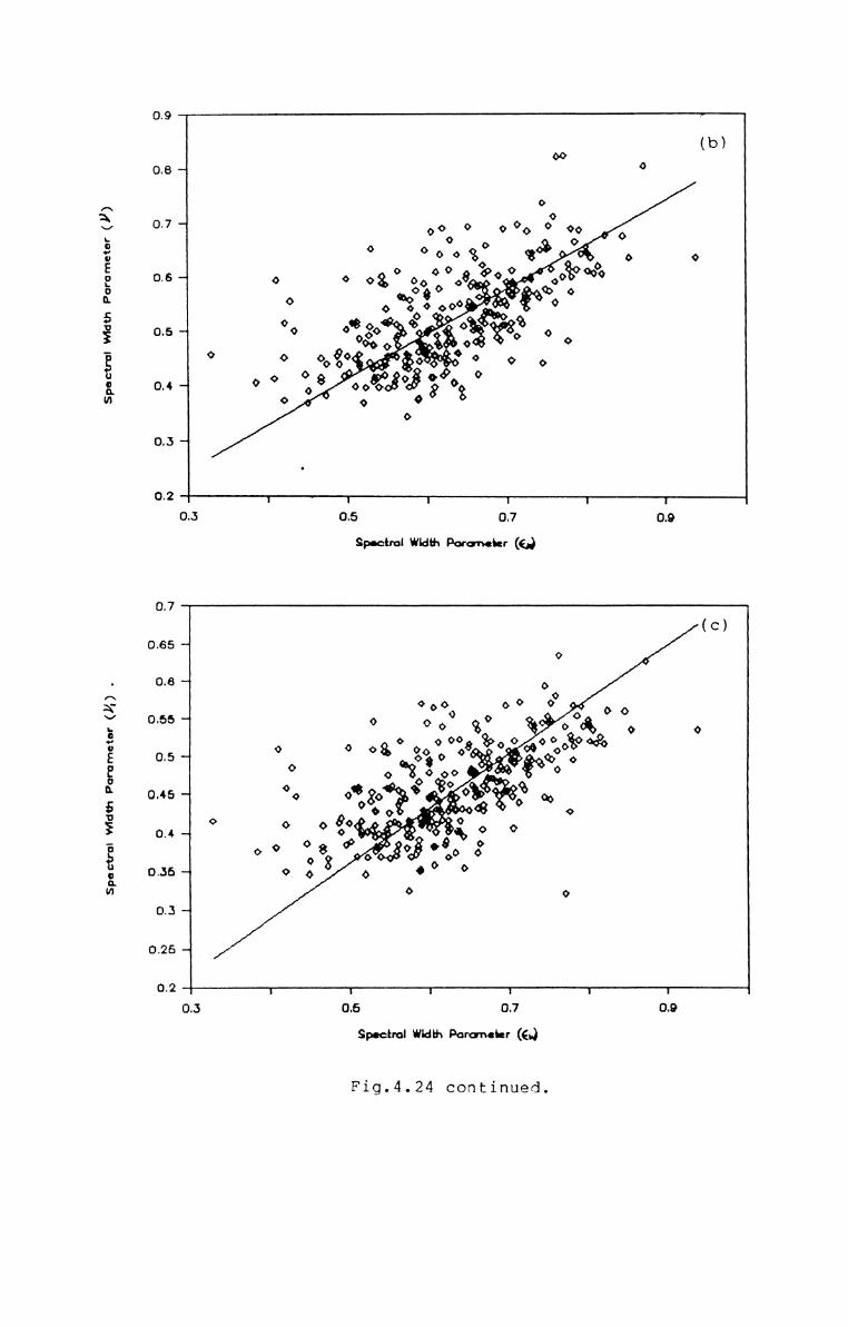
Spectral Math Parameter (V)

Spectral Width Parameter .

0.9

0.8

0.7

0.6

0.5

0.4

0.3

0.2

0.7

0.65

0.6

0.55

0.5

0.45

0.4

0.35

0.3

0.25

0.2

0.3I I I0.5 0.7Spectral Width Porcrnehr

0.9

0.3I I I0.5 0.7

Spectral Width Paraneter (6,)

Fig.4.24 continued.

0.9

During these months the waves are generally high associatedwith comparatively lower periods and spectral widths. During

October-April the waves are of lower heights associated withcomparatively higher periods and spectral widths. Hence,May-September may be classified as the rough season andOctober-April may be classified as the fair season (of waveclimate) for this location. During the rough season thewaves generated in the Arabian Sea, and during the fairseason those generated at two different and far-away loca­tions constitute the wave climate in this area. A detailedstudy involving generation, propagation and directionalspreading is required to identify these generating areas.

The spectral peakedness parameter Qp cannot be taken asa measure of the width of the spectrum in shallow waters dueto the presence of multiple-peaks in most of the shallowwater spectra. The spectral width parameters e .V and 1/1S’

exhibit characteristic properties during the rough as wellas the fair seasons. These parameters can be useful inestimating the sea state in shallow waters where swells aredominant.

The parameters computed from the average spectra agreewell with the average of the spectral parameters sampled at1 per day. Decrease in slope of the high frequency side ofthe spectrum with increasing energy is observed with the

110

monthly average spectra. The relation between slope andenergy of the spectrum can be determined from Eq.(4.6). Thespectral width parameters are dependent mutually as well asto the peak period through Eqs.(4.7-4.10).

The statistical height parameters show very high corre­lation between each other, which can be represented byEqs.(4.ll-4.12). The ratio Hsw/§ is about 7% less than thetheoretical value based on Rayleigh distribution of waveheights. The different statistics of periods exhibit varying

degrees of correlation, among which T2 and T8 are bettercorrelated. The relation between the period parameters canbe represented by Eqs.(4.l3-4.14). The period parameters arealso related to the peak period/frequency through Eqs.(4.15­4.17). The peak frequency, which is usually employed inalmost all the applications, can be computed from the signi­ficant wave period using Eq.(4.l8).

The spectral width parameters derived from spectral andzero-crosssing analyses deviate from each other, owing tothe differences/limitations of tflme methods. As thespectrally obtained parameters)/and.U1 are statisticallymore stable, and are better correlated to ew, they may beused for practical purposes. However, only one of them needbe considered, since they are related through E2q.(4.2) bydefinition.

lll

CHAPTER 5

WAVE SPECTRAL MODELS

The individual wave spectra computed from the recordeddata are compared with different spectral models suggestedfor shallow water conditions. A new empirical model isderived for shallow water applications and is verified withthe measured spectra. The other theoretical shallow waterspectral models selected for this study are theKitaigorodskii et al. spectrum, the TMA spectrum in itsoriginal form and with certain modifications, the Wallopsspectrum and the GLEIRL spectrum. Since the Scott spectrum

and its modified flown (Scott-Weigel spectrum), thoughoriginally derived for deep water conditons, has found itsapplication in many shallow water conditions also (Ch.2),these models are also selected.

5.1. DERIVATION OF A SHALLOW WATER SPECTRAL MODEL

Most of the shallow water spectral models are derivedfrom some deep water models by applying a shallow waterdispersion relatioship. For example, Kitaigorodskii et al.(1975) applied 51 dispersion relationship ix) Phillips‘spectral model to arrive at an new shallow water model andBouws et al. (1985) applied the relationship derived byKitaigorodskii et al. on the JONSWAP model to derive the TMA

spectral model. ‘The JONSWAP spectrum which ii; hi fact the

112

modification of the P-M spectrum for the conditions ofgrowing seas may be suitable for similar conditons in theshallow water when the appropriate dispersion relationshipis applied. The shallow water spectra, generalby, are notrelated to the local wind conditions. That is, the shallowwater wave spectra result from the waves generated at someother locations and propagated towards the coast and arethus swell dominated. In such a case, a better modelsuitable for transformation to shallow water conditions willbe one which is able to predict the deep water saturated seastate successfully. The P—M spectrum is one such modelsupported by various field and laboratory data for itsability to simulate the spectra of deep water saturated seaconditions. The functional form of this model is given as

s(f) = o\g2(2‘IT)"4 f’5 exp [-(5/4)(f/fm)"4] .....(2.13)

By incorporating the finite depth dispersion parameter pro­posed by Kitaigorodskii et al. (1975) in the P-M spectrum,the shallow water model, which may be called Pierson­Moskowitz-Kitaigorodskii (PMK) spectrum, can be obtained as

.. 2 "4 ‘S __ *4 Q)s<f> - o<g (277) f exp [ <5/4><f/£m> 1a>< h)...(5.1)

The function mauh) is dimensionless and varies monotonouslyfrom 1 in deep water to 0 in depth h=0. It is expressed as

(I;-kw hyz (DQTTE (h/g)1/2.} .....(2.26)113

For shallow waters CD(U.)h) is less than 1 and in such casesthe function is well approximated by

auwh) -_- 1/2 (ugh) 2 .....(2.27)By applying this approximation, Eq.(5.1) becomes

S(f) = 0.5O(g2(2TT)'2f’3 exp I-(5/4)(f/f6)-4].....(5.2)

If the dispersion relationship of Kitaigorodskii et al.is valid, the PMK spectrum (Eq.5.2) must be able to predictthe swell dominated shallow water wave spectra. Validationof this model is carried out alongwith the other models.

5.2. COMPARISON OF MEASURED SPECTRA WITH MODELS

Typical examples of spectra predicted by differentmodels corresponding to an observed spectrum are given inFig.5.l. There_is no standard test, till date, to examinethe fitness of a theoretical spectral model to the observedspectrum. The procedure followed in almost all the studiesin the past is to make a visual comparison. This ispossible when the number of observed spectra and the numberof models to be tested are limited. As the number of dataand models are large in the present study, the deviationindex method suggested by Liu (1983) is adopted for testingthe goodness of fit. The deviation index is given by

DI = 22[(S(fi)-ST(fi))*1OO/S(fi)] [S(fi)¢§f/E]....(S.3)

114

Sp octrul Donotty (mac)

Sp octrol Don sky

2.01.91.8‘1.7 '11.6-‘1.5"‘1.4-‘1.3"‘1.2"1.1 "1.0-‘

0.8 -<

0.7 10.6 ­0.5 -4OJ —0.3 -<

0.2 ­0.1 ­0.0 -4

l

1l_JLJJ

.°.°.°.°.0.“':".".":‘.“.".":":‘!° mo~Am<oo—-u+c.no:~Jcnoo JLIILJ

00.00 areas

11

.0 0 1

0.2 0.4

Frequency (Hz)-— 1 + 6 0 7 A 8observed, 2: Jensen's, 3: Scott, 4: Scott-Weigel,

: PMK, 6: TMA with average JONSWAP parameters,TMA withcxV,and JONSWAP parameters, 8: TMA (original),TMA with computed Y and CXV, and 10: Wallops spectrum.\0\lU1+-4 0000

Fig.S.1 Typical examples of spectra predicted by djfferentmodels corresponding to an observed spectrum.

where S(fi) and ST(fi) are the measured and theoreticalspectral densities at frequency fi. E is the total energyof the observed spectrum and Af is the frequency intervalused in calculating the spectrum. ‘This deviation index isactually the sum of percentage deviations of the theoreticalspectral densities from the observed ones weighted by therelative magnitude of the observed spectral density. Aperfect representation will yield a zero DI and hence asmaller DI implies a better fit. No criterion isestablished for the acceptance/rejection of a model based onthe value of [H3 Hence a criterion for the acceptance orrejection of a model is fixed based on the placement of thetheoretical spectrbm with respect to the confidence limits.The upper and lower confidence limits of the observedspectra are calculated at the 0.05 level of significance. Amodel is considered to fit the measured spectrum when the DIvalue of the model is less than the DI value of lowerconfidence limit (DILC) with respect to the observedspectrum.

In addition to the application of the ‘Deviation Index’to examine the fitness of models, total energy, peakfrequency and peak energy density derived from the modelsare also compared with the observed values to determine theapplicability of the different models.

115

5.2.1. Jensen's Model

The spectral model suggested by Kitaigorodskii et al.(1975) depicts the high frequency side of the spectrum only.

Hence the slope of the high frequency side is the onlyparameter that can be compared. Jensen (1984) modifiedthis model tn; adding the low frequency face (Eq.2.3l)assuming the original form for the high frequency tail.

The DI values for this model range from 37 to very highvalues like 70,000. The higher values correspond to the lowwave heights. This model is found to fit the data in only 4cases, which is dnly 1.26% of the total records used for thestudy. Those 4 cases which fit the observed spectracorrespomd to the high energy conditions (H > 1.8 m)8

associated with lower wave periods (T < 11 s). The casesP

with Tp higher than 10 s fit in when HS is about 2.5 m. Inthis model, the energy density is a function of the peakfrequency and hence as the peak period increases, the energy

also increases in the order of TD3 (Eq.2.3l). The fittingof this model to the higher waves is indicative of thevalidity of the power law of T in the high energyD

conditions. The total energy and peak energy density predic­ted by this model are depicted in Fig.5.2 (a-b). Theenergies are over-estimated in most of the cases, theaverage ratio being > 50. From these figures also it can be

116

seen that the energy and S(fm) predicted by this modelbecome closer to the observed values only when the energy of

the observed waves are high (H8853 2.5 m).

5.2.2. TMA Spectrum with Phi1lip's Constant OT and AverageJONSWAP Parameters

The TMA spectrum in its original form requires the 5free parameters to be derived from the observed spectrum.If some useful averages are available for the scale andshape parameters,0(J, Y , J3 and 6b, the number of freeparameters is reduced to fm and hence the application ofthis model becomes easier. So the TMA spectrum with

Phillips‘ constant as the scale parameter and averageJONSWAP values of shape parameters ( 1/: 3.3, (5 = 0.07 anda

6b = 0.09) is tried.

The DI values are found to be very high in most of thecases. They range from 33 to more than 89,000. As in the

case of Jensen's spectrum, the higher values correspond tothe lower wave heights. This model fits only in 63 cases,out of which 4 are the same as that fits the Jensen'sspectrum. The total energy and S(fm) predicted by this modelare depicted in Fig.5.3 (a-b). The values are overestimatedmany times. Here also the energy densities are functions offm and the model resembles with Jensen's.

117

5.2.3. TMA Spectrum with Scale Factortxiv and AverageJONSWAP Parameters

The TMA spectral model assumes the scale parameter CX‘]as a function of the observed spectral density. Vincent(1984) in his study showed that this coefficient is afunction of the steepness (Eq.2.36). Considering thisobservation, Phillips‘ constant in the form tried in theabove section is replaced withcf V and the spectrumcorresponding to each observed ones are computed. Thevalues of OVV range from 0.000015 to 0.013. Large variationin the values around the mean 0.0016, as shown by thestandard deviation of 0.0023, with a mean of 0.0016.

1

This form presents a bettertfit with the data. The DIvalues for this model are found to be considerably lower(29-114) compared txa that obtained with time Phillip'sconstant as scale parameter. This observation is inconfirmation to the observation of Vincent (1984) that thescale parameter is proportional to the steepness rather thanbeing a constant. The DI values are always lesser than theDIs corresponding to the upper confidence limit spectra.They are less than DILC in 58 cases which contribute 18.3%of the total. This is found to have the best fit to spectrawith lower peak periods. However, at low T this givesP

better fit in the lower height ranges also. The total energy

118

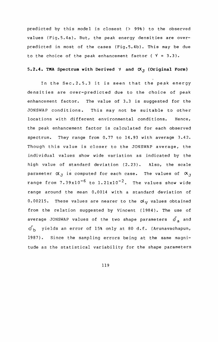
predicted by this model is closest (> 99%) to the observedvalues (Fig.S.4a). But, the peak energy densities are over­predicted in most of the cases (Fig.5.4b). This may be dueto the choice of the peak enhancement factor ( Y = 3.3).

5.2.4. TMA Spectrum with Derived ‘Y and CXJ (Original Form)

In the Sec.2.5.3 it is seen that the peak energydensities are over—predicted due to the choice of peakenhancement factor. The value of 3.3 is suggested for theJONSWAP conditions. This may not be suitable to otherlocations with different environmental conditions. Hence,the peak enhancement factor is calculated for each observedspectrum. They range from 0.77 to 14.93 with average 3.42.Though this value is closer to the JONSWAP average, theindividual values show wide variation as indicated by thehigh value of swandard deviation (2.23). Also, the scaleparameter (X3 is computed for each case. The values of (XJrange from 7.39xl0"6 to 1.21x10'2. The values show widerange around the mean 0.0014 with a standard deviation of

0.00215. These values are nearer to the CXV values obtainedfrom the relation suggested by Vincent (1984). The use ofaverage JONSWAP values of the two shape parameters cia and

cfb yields an error of 15% only at 80 d.f. (Arunavachapun,1987). Since the sampling errors being at the same magni­tude as the statistical variability for the shape parameters

119

P R E D I C T E D

0' .12 (a) 7(b)30 ‘. '1can» 90 0 b O0.8 20-13; .0 O O0. o o _‘

O ope o .0 0 0 0 0 0‘ ‘ ° ‘4. 3"’ . ..‘.o.' ' ' I’ ‘ix r03 'O-O --- f V Y 7 ' V Oo.o 0-: 0-2 06 N­Fig.5.2 Plot of computed (a) energy and (b) peak energydensity against measured: Jensen's model.

40

(3.0 2- 0 41:0 V 5'0Fig.5.3 Plot of computed (a) energy and (b)

against measured: TMA model with oCJONSWAP parameters.

peak energy densityand average‘(a) ‘(b)

0.0 0.; 0-2 0.3 0-4" 0-0 2'0 4'0 6'0O B S B R V E D

Fig.5.4 Plot of computed (a) energy and (b) peak energy dendityagainst measured: TMA model withcfiv and average

JONSWAP parameters.

(x———*1:l correspondence;A————~aupper confidence limit= and w———-vlower confidence limit)

(Arunavachapun, 1987), the average JONSWAP values of the two

shape parameters cia and cib (0.07 and 0.09 respectively)are used in the computation of spectra using this model.

The DI values obtained with this form vary between 20and 94 only, indicating a better fit to the observed spectrain most of the cases. In 169 cases (53.3%),'the DI valuesare less than DILC. In the higher energy conditions (Hss >1.4 m) it gives DIs lesser than the DILC. In the lowerenergy conditions the fitness is not as good as the cases ofhigh energy conditions. The lesser fit in this range may bedue to the existence of major secondary peaks in the lowerenergy cases, which make the squared deviation larger. Thetotal energy is underestimated by about 30% by this model(Fig.5.Sa). However, the peak energy density is simulatedcorrectly (Fig.5.5b). This indicates that it is the shapeparameter that.requires modification to obtain a betterestimate of the total energy. But as the peak energydensity is estimated correctly the choice of peakenhancement factor 7’ is in order. The average value of 7’

for the cases where the DI values are lower than DILC is3.0. Then it is the shape parameter <J; and b that causesunderestimation of energy densities at the tails of the

(XJ, ‘Y , Cf and 6b have to bespectrum. That is, f ami

defined from the observed spectrum. In other words, thespectrum has to be fully defined apriori.

120

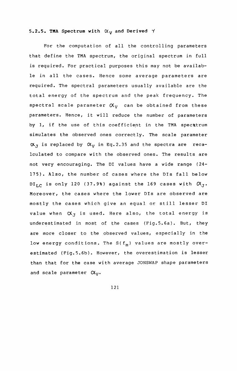
5.2.5. THA Spectrum with (XV and Derived ‘V

For the computation of all the controlling parametersthat define the TMA spectrum, the original spectrum in fullis required. For practical purposes this may not be availab­le in all the cases. Hence some average parameters arerequired. The spectral parameters usually available are thetotal energy of the spectrum and the peak frequency. Thespectral scale parameter CXV can be obtained from theseparameters. Hence, it will reduce the number of parametersby 1, if the use of this coefficient in the TMA specxtrumsimulates the observed ones correctly. The scale parameter

CXJ is replaced by (Xv in Eq.2.35 and the spectra are reca­lculated to compare with the observed ones. The results arenot very encouraging. The DI values have a wide range (24­175). Also, the number of cases where the DIs fall belowDILC is only 120 (37.9%) against the 169 cases with (XJ.Moreover, the cases where the lower DIs are observed aremostly the cases which give an equal or still lesser DIvalue when CXJ is used. Here also, the total energy isunderestimated in most of the cases (Fig.5.6a). But, theyare more closer to the observed values, especially in thelow energy conditions. The S(fm) values are mostly over­estimated (Fig.5.6b). However, the overestimation is lesserthan that for the case with average JONSWAP shape parameters

and scale parameter CXV.

121

5.2.6. Wallops Spectrum

The Wallops spectrum redefines the scale parameter flas an internal parameter from the total energy of thespectrum as is done in Vincent (1984). Also, it defines avariable exponent, m, of the frequency, as a function of thetotal energy, instead of a fixed value assumed in othermodels. Hence the number of parameters is limited to 2 as

against 5 in the TMA spectrum. The values of fl range from4.57xlO'6 to 6.24x10-3. The value of m vary from 1.0 to14.5, the average being 5.6. The variations observed in the

values of ,8 and m are large. Since ,3 and m are functionsof the energy, variation in accordance with the variation ofthe energy can be expected.

This model fits the observed data well irnaa largenumber of cases. The values of DI range from 17 to 278.The average DI is 56 but there is wide variation in thevalues as indicated by the standard deviation of 25. In 120

cases the DI values are lower than DILC. As observed fromthe DI values, this model gives better fit where HS is above0.75 m. In this range (HSS is 10.75 m), the DI values arelower than DILC in 81 cases (67%) of the total of 121cases. The total energy is estimated almost correctly butare overestimated in a few cases where T is high (Fig.P

5.7a). The large deviations foumd in the high energy cases

122

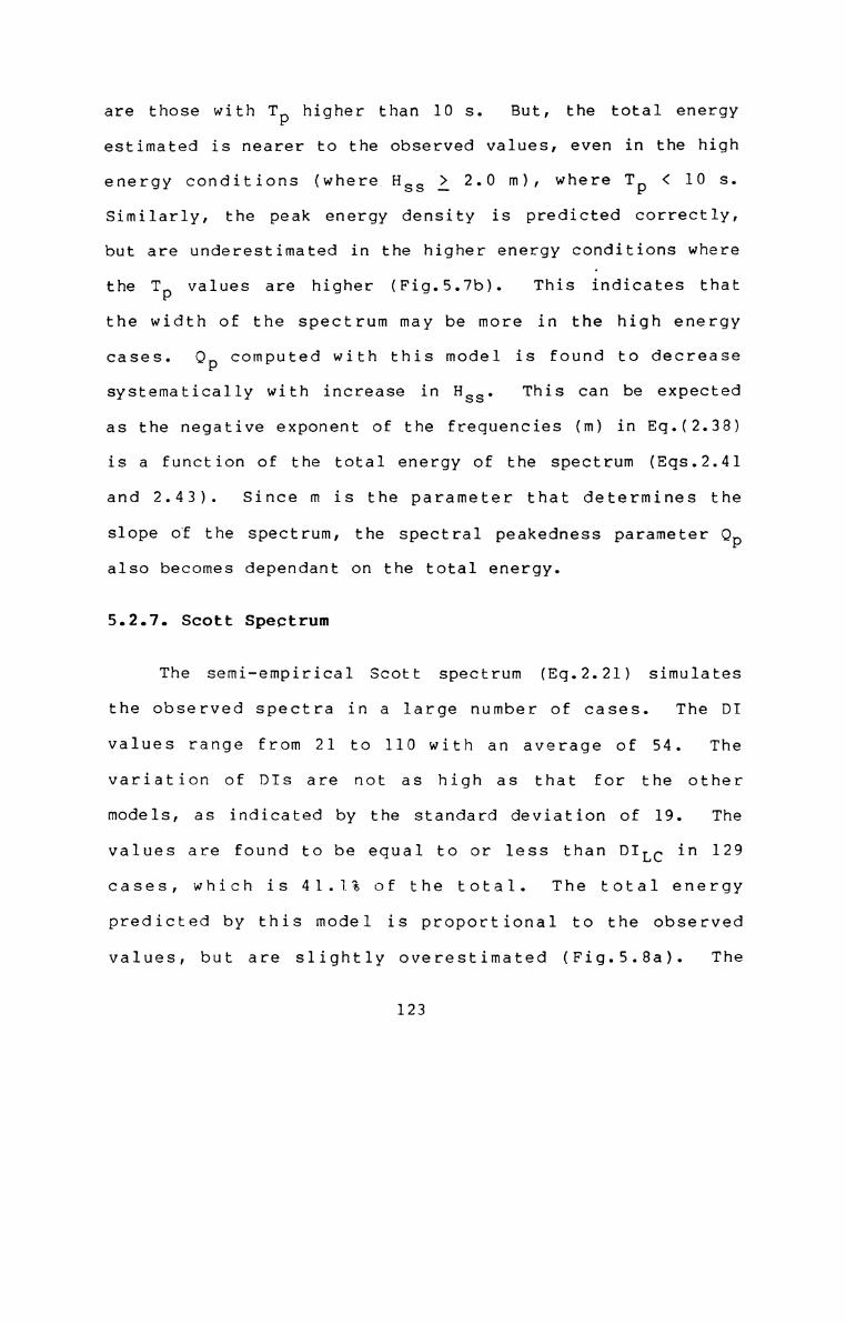
are those with Tp higher than 10 s. But, the total energyestimated is nearer to the observed values, even in the high

energy conditions (where H53 3 2.0 m), where Tp < 10 s.Similarly, the peak energy density is predicted correctly,but are underestimated in the higher energy conditions where

the Tp values are higher (Fig.5.7b). This indicates thatthe width of the spectrum may be more in the high energycases. Q computed with this model is found to decreaseP

systematically with increase in Fl This can be expectedss°

as the negative exponent of the frequencies (m) in Eq.(2.38)is a function of the total energy of the spectrum (Eqs.2.41and 2.43). Since m is the parameter that determines the

slope of the spectrum, the spectral peakedness parameter Qpalso becomes dependant on the total energy.

5.2.7. Scott Spectrum

The semi-empirical Scott spectrum (Eg.2.21) simulatesthe observed spectra in a large number of cases. The DIvalues range from 21 to 110 with an average of 54. Thevariation of DIs are not as high as that for the othermodels, as indicated by the standard deviation of 19. Thevalues are found to be equal to or less than DILC in 129cases, which is 41.1% of the total. The total energypredicted by this model is proportional to the observedvalues, but are slightly overestimated (Fig.5.8a). The

123

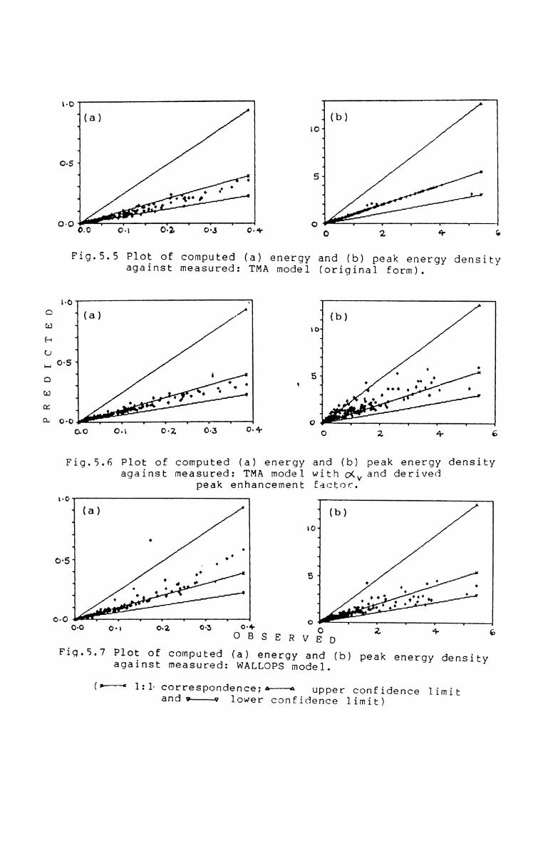
PREDICTED

\-O

0-0 1+ 5da4

0.0

Fig.S.5 Plot of computed (a) energy and (b) peak energy densityagainst measured: TMA model (original form).

O-5 ‘

1

O O

9 o

Fig.S.6 Plot of computed (a) energy and (b) peak energy densityagainst measured: TMA model with oyvand derived

peak enhancement factor.

01 '

O

*4‘ A44 1 A A I J J J.00'3 0'4‘ 0O B S E R V B D

Fig.5.? Plot of computed (a) energy and (b)against measured: WALLOPS model.

6.2.

peak energy density

(*—** 1:} correspondence;a~——«and v-———-—v . upper confidence limitlower confidence limit)

S(fm) values, on the other hand, are overestimated by about78% (Fig.5.8b). This may be due to the higher peakedness ofthis model due to the higher negative exponent (-5) of thefrequency assumed in its derivation.

5.2.8. Scott-Weigel Spectrum

The Scott-Weigel spectral model (Eq.2.22) with thevariable coefficients (A and B), which are functions of thetotal energy of the spectrum, is also found to simulate thespectra better than the Scott spectrum. The DI valuesrange, in this case, from 20 to 99 with an average of 53 anda standard deviation of 18. The values are slightly lowerthan the corresponding values for Scott spectrum, indicatinga better fit than the Scott spectrum. However, the number

of cases in which the DI values are lower than DILC is onlyone less than that for the Scott spectrum. Simulation bythis model is found to be better in the high energyconditions compared to the Scott spectrum. This is madepossible by the choice of the values for A and B accordingto the energy of the spectrum. This choice also makes thepredicted total energy closer to the observed (Fig.5.9a).Here also, the values of S(fm) are over-predicted in mostcases (Fig.S.9b). But the rate of over-prediction is lesscompared to the Scott spectral model, especially in the highenergy conditions. In the cases where the energy is very

124

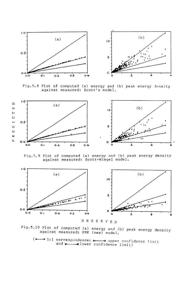
PREDICTED

A L J._ 1 1 1 1 L 1

Fig.5.8 Plot of computed (a)against measured:

energy and (b) peak energy densityScott's model.

9o

Fig.S.9 Plot of computed (a) energy and (b) peak energy densityagainst measured: Scott-Wiegel model.

OBSERVEDFig.5.1O Plot of computed (a) energy and (b) peak energy densitagainst measured: PMK (new) model. Y

(“"*’l’1 C°rreSP0”de0C€;4b———jAupper confidence limitand‘w————vlower confidence limit)

low the values are predicted almost correctly. The correctsimulation of total energy and lesser over-prediction ofS(fm) indicate that the peakedness is higher, as discussedin the Sec.5.2.7, but it is seen that the values areconsiderably modified from the Scott model.

5.2.9. PHK Spectrum

The PMK spectrum (Eq.5.2) with Phillips‘ constant asthe scale parameter simulated the observed spectra correctlyin the high energy conditions only. The DI values rangefrom 27 to more than 46,000. The energy densities are over­

estimated in the low energy conditions. DI values £ DILC isobtained in 11 cases only, which correspond to Hs > 1.9 m.

When the scale factor (X is replaced by CXV better fit isobtained in a large number of cases, as shown by the DIvalues which range from 23 to 98 only. The average DI is 54with a standard deviation of 16. This shows a fit betterthan the Scott spectrum. The DI values are lower than DILCin 114 cases. The total energy is proportional to themeasured, but are underestimated (Fig.5.10a). The peakenergy density is also underestimated (Fig.5.l0b). Thisindicates that the scale factor may be low and requiresmodification.

125

The peak frequencies estimated by this model is foundU: be shifted tx> the higher frequencies. The variation islinear and is estimated to be about 7%. This is theinfluence of the dimensionless function (D(C.Uh) which actsmore strongly cum lower frequencies than (N1 higher frequen­

cies, As a result, the spectral density estimated by the PMspectrmn is reduced more cum the lower frequencies and thereduction 1h; less <m1 succeeding frequencies. Consequentlymaximum density is attributed to a frequency higher than the

actual fm which is an input to the model. This can becompensated by applying a peak enhancement factor, as donein the case of JONSWAP spectrum. If the peak enhancementfactor of the JONSWAP model is adopted here in this model,

this becomes the TMA spectrum modified with CXV (Sec.5.2.6).It is already seen that this modified form does not fit wellwith the data, it underestimates the total energy and over­estimates the maximum energy density. Another way tocompensate for the shift in fm is to apply a factor to thecoefficient of the exponent, so that the estimated energydensities will be higher. This will enable the enhancementof the underestimated total energies and the peak energydensities. It is seen that the factor -3/4 (in place of ­5/4 in the PM spectrum) can simulate fm correctly. The PMKspectral model is modified in this line and the simulatedspectra are compared with the average spectra computed for

126

the different height and period ranges. The results ofcomparison of this model alongwith other models are given inthe following section.

5.2.10. GLERL Model

The GLERL spectral model (Eq.2.49) is based on manyempirical constants, the determination of which iscumbersome. A few cases were computed and it is found thatthe determination of these constants by repetetive iterationtakes much time in an IBM PC/XT computer. Moreover, thefitness of this model with the data is very poor in the fewcases tested. Hence, a detailed analysis is not attempted.

5.3. COMPARISON OF AVERAGE SPECT.‘RA WITH MODELS

The average spectra at HSS intervals of 0.25 m and Tpintervals of l s also show characteristics similar to thatobserved with the individual spectra (Sec.5.2), in thecomparison with models. The DI values obtained with theseaverage spectra are lower than those obtained in the case ofindividual spectra. The values obtained for the differentmodels are presented in Table 5.1. The TMA spectrum givesthe lowest range of DI values and the variation is also theleast, as shown by the standard deviation, for this model.This is followed by the PMK spectrum with the modifiedcoefficient for exponent (here after will be referred as PMK

127

Table 5.1 DI Values of Spectral Models for H88-Tp Range Spectra

No’ 0c LC PHK scor SCT-H JENS THAJ THAJV TMA THAV1 133.3 45.0 78.6 87.9 82.7 4718.5 3579.8 74.0 62.9 112.22 132.5 44 8 68.4 99.5 88.6 3965.4 3041.7 81.3 63.0 94.63 132.3 44.7 27.7 51.5 33.5 8718.0 6796.4 41.0 36.0 35.84 133.2 45.0 32.1 48.8 38.3 14183.5 11137 3 49.6 41.9 44.25 133.7 45.2 33.5 42.0 44.1 18081.5 14367.7 53.7 42.8 49.26 134.3 45.4 38.4 37.9 59.0 28476.8 23081.3 65.1 47.1 58.27 132.0 44.6 55.9 78.0 70.1 1443.4 1100.9 66.4 49.6 69.98 132.6 44.8 34.3 57.6 47.2 1672.7 1292.1 52.4 41.9 44.89 132.4 44.7 30.6 42.0 41.0 2870.5 2228.1 45.1 37.8 42.0

10 132.3 44.7 26.8 49.1 33.6 3401.7 2657.0 45.7 36.8 36.511 133.2 45.0 30.7 36.8 44.4 5756.9 4561.8 47.4 40.1 45.512 133.5 45.1 32.8 37.7 33.2 10474.2 8481.7 55.6 37.6 42.413 132.0 44.6 38.3 68.0 48.3 402.0 294.9 44.5 43.0 42.114 132.8 44.9 60.8 92.1 78.3 558.3 428.0 71.3 59.2 75.115 132.8 44.9 64.3 67.2 69.1 1233.1 950.5 71.7 54.4 73.216 132.6 44.8 40.5 47.9 47.8 926.2 707.6 50.9 36.4 47.817 132.5 44.8 22.7 44.2 30.5 1786.5 1385.9 38.7 33.4 32.318 132.8 44.9 34.5 39.0 41.6 2296.1 1810.5 49.1 43.6 53.319 132.7 44.8 27.4 33.6 39.1 3513.8 2833.2 49.2 35.4 38.720 132.0 44.6 68.4 91.2 83.3 226.5 178.8 76.7 61.2 90.921 131.9 44.6 50.0 55.8 46.0 259.7 185.4 51.9 52.6 61.022 136.7 46.2 76.4 79.8 81.0 421.8 322.6 81.1 67.9 129.823 132.4 44.7 32.5 54.5 42.0 356.8 263.2 51.5 42.6 43.224 132.4 44.7 25.6 40.8 33.6 473.0 354.6 37.6 29.1 32.725 131.9 44.6 50.5 30.7 25.1 669.9 506.6 29.0 22.4 21.326 132.6 44.8 29.2 32.2 43.2 1175.9 924.3-44.7 37.0 43.527 133.1 45.0 32.7 32.7 38.6 1378.9 1102.4 54.9 37.7" 45.528 133.0 45.0 60.6 76.6 72.4 127.3 102.0 68.4 52.3 70.729 132.0 44.6 50.1 47.9 47.1 233.0 176.4 53.7 41.3 54.930 132.4 44.7 27.0 42.3 34.5 314.8 '237.6 43.9 34.5 35.931 132.4 44.7 21.2 25.7 17.4 446.7 332.9 29.7 21.9 24.032 132.3 44.7 21.8 26.2 21.9 686.0 532.9 41.2 27.8 29.533 132.0 44.6 37.0 45.2 32.8 831.6 659.6 61.4 38.7 -38.834 132.4 44:7 57.6 72.1 65.8 87.7 74.9 63.1 49.2_ 73.035 132.4 44.7 44.5 65.1 57.4 110.8 86.8 55.5 39.5 53.136 132.5 44.8 35.9 43.8 38.1 130.6 97.3 43.1 36.5 41.737 132.3 44.7 17.3 45.8 32.4 201.5 147.0 36.8 26.7 27.538 132.2 44.7 22.6 34.3 25.2 256.1 188.9 37.3 28.8 28.839 132.9 44.9 53.6 69.9 57.0 510.7 396.3 65.0 43.3 43.840 132.3 44.7 30.8 43.1 34.5 75.4 55.8 40.7 36.4 37.341 132.7 44.8 45.4 44.1 40.9 108.4 86.8 48.0 38.1 52.442 132.8 44.9 36.1 43.0 36.7 168.9 127.6 49.4 38.4 43.743 132.0 44.6 26.6 45.0 33.8 300.8 222.0 42.9 30.5 30.044 132.6 44.8 60.1 64.5 49.3 663.9 540.8 78.2 42.8 42.945 132.9 44.9 48.9 68.1 59.4 49.5 47.0 54.7 45.9 55.046 132.7 44.8 48.7 32.5 29.9 36.1 37.1 36.9 33.7 45.247 132.2 44.7 37.2 43.6 37.9 60.0 49.7 45.2 34.6 40.448 132.1 44.6 18.0 46.2 30.5 92.0 63.5 38.1 23.9 23.849 132.8 44.9 28.5 48.2 34.8 187.5 137.0 50.8 33.0 33.750 132.3 44.7 25.3 48.3 42.3 40.9 36.6 38.2 32.4 32.251 132.3 44.7 20.9 44.6 38.0 67.5 51.6 41.4 27.9. 28.752 133.2 45.0 41.5 70.4 65.0 47.6 51.1 53.4 45.4 46.653 132.5 44.8 19.3 46.4 39.9 42.3 35.9 37.9 25.5 25.4

Max° 136.7 46.2 78.6 99.5 88.6 28476.8 23081.3 81.3 67.9 129.8Min: 131.9 44.6 17.3 25.7 17.4 36.1 35.9 29.0 21.9 21.3Avg: 132.7 44.8 38.5 52.1 46.0 2364.5 1870.7 51.6 40.0 48.4s 0: 0.7 0.2 14.8 17.6 16.9 5056.0 4058.1 13.0 10.5 21.5

I For corresponding H and T ranges see Table 6.1.For expansion of abggeviatigns, see overleaf.

Expansion of Abbreviations in Table 5.1

UC

LC

PMK

SCOT

SCT-W

JENS

TMAJ

TMAJV

TMA

TMAV

WLP

Upper confidence limit spectrum

Lower confidence limit spectrum

PMK spectral model

Scott's spectral modelScott - Weigel spectral modelJensen's modification of theKitaigorodskii et al. spectrumTMA spectral model with averageJONSWAP scale and shape parameters

TMA spectral model with Vincent'sscale parameter and averageJONSWAP shape parameters

TMA spectral model in originalform

TMA spectral model with Vincent'sscale parameterWallops spectral model

spectrum). TMA spectral model with computed 7’ and CXV andthe Wallops model show the widest range of DI values.

As seen in Sec.S.2 the TMA spectrum in its originalform has the DI values lower than the DILC in maximum numberof cases (75%). This is followed by the PMK model with 69%

of cases having DI values lower than DILC. The Scott-Weigelin 62%, TMA with CXV in 58% and Scott and Wallops in 40%

each of the cases tested have DI values lower than DILC. TheTMA model with the average JONSWAP parameters and O<V as thescale parameter fits the data in a very few cases only. In36% of the cases the DI values are lower than DILC.

The total energy estimated by the models is presentedin Fig.5.ll (a-g). ‘The energy is estimated close to theobserved values by a few models. The Scott-Weigel model

estimated the values ranging‘ from 0-19% over the observedvalues. On an ‘average the values are overestimated by 2%only. This model is followed by the Scott model whichpredicted the values in a range varying from 29-156% of theobserved values with the average 4% higher. Tflua TMA model

with average JONSWAP shape parameters and Ckv as scaleparameter estimated the values in the range 84-111% with theaverage 4% less than the observed. The PMK model estimated

the values in the range 84-101% of the observed with averageunderestimated by about 5%. The original TMA model under­

128

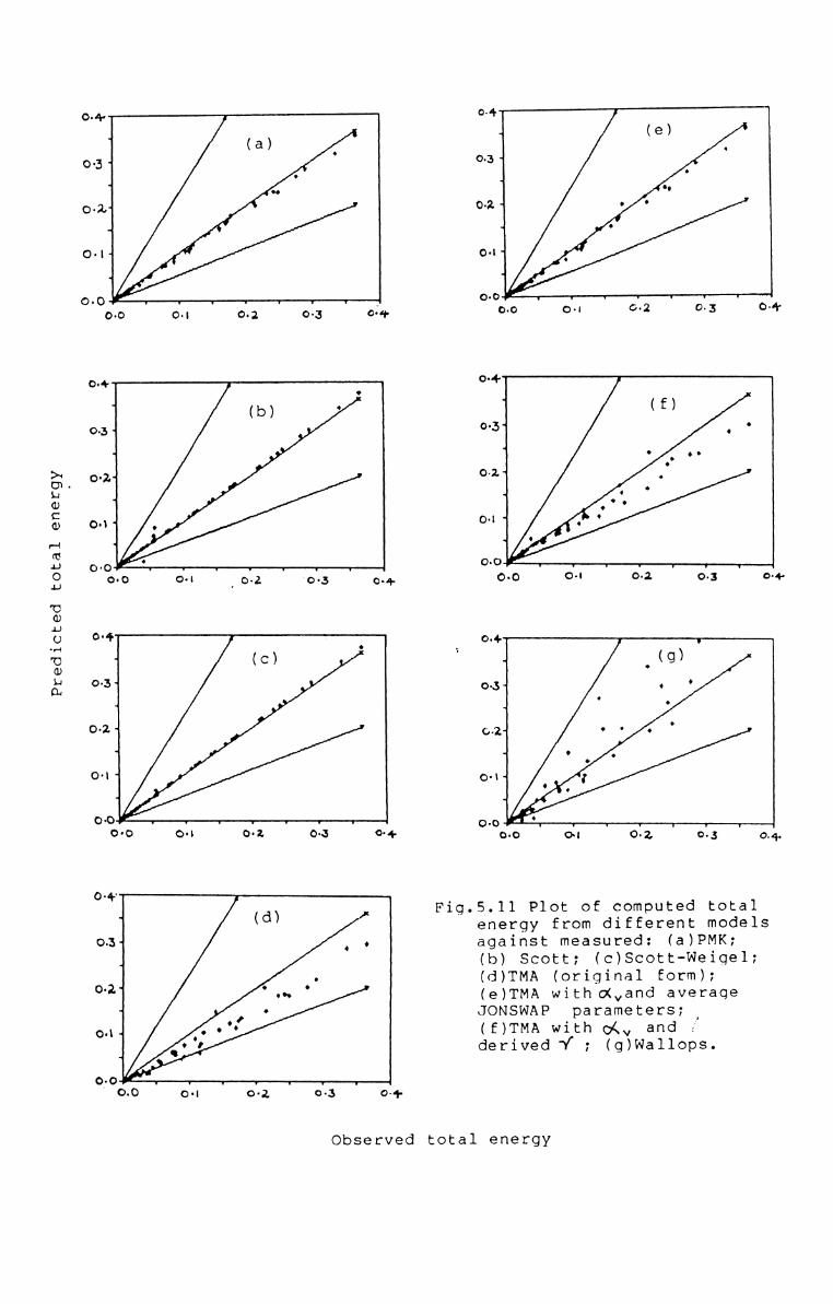
Predicted total energy

observed

0-! O-4­

Fig.S.11 Plot of computed totalenergy from different modelsagainst measured: (a)PMK;(b) Scott; (c)Scott-Weiqel;(d)TMA (original form);(e)TMA withcxvand averaqeJONSWAP parameters;(f)TMA with okv and .derived'Y ; (g)Wallops.

total energy

estimated the energy by about 31%. This model with the scale

factor O(v estimated the values in a range varying from 75­148% of the observed with the average about 8% lower thanthe observed. The energy predicted by the Wallops modelshow wide variability (26-380%). The Values are found to beoverestimated at high energy conditions. The Jensen's formof the Kitaigorodskii et al. spectrum and the TMA model withaverage JONSWAP parameters highly overestimated the energyin most of the cases.

The peak energy densities predicted by the differentmodels are plotted against the observed values in Figs.5.12(a-g). The TMA model is found to estimate the valuescorrectly. The Wallops model also simulated the peak well,but with scatter. The values are found to be slightlyoverestimated in those cases with lower peak energy densi­ties and underestimated in the high peak energy densitycases. This model predicted the values in the range 37-265%of the measured values with the average overestimated byabout 18%. The PMK model underestimated the values, at 47­195% of the measured, with the average about 14% lower thanthe measured. All the other models overestimated the peakenergy densities by about 40% or more.

129

Predicted peak energy density

Fig.5.12 Plot of computed peakenergy density from variousmodels against measured:(a)PMK; (b) Scott;(c)Scott-Wiegel; (d) TMA(original form); (e) TMAwithcxv and average JONSWAPparameters; (f) TMA withcxvand derived Y ; (g)Wa11ops.

Observed peak energy density

5.4. A DISCUSSION ON THE SCALE FACTOR

In order to define the spectrum, different models adoptdifferent scale parameters. In Kitaigorodskii et al. andJensen's forms the Phillip's constant (o() is used as thescale factor. The TMA model assumes the scale factor of the

JONSWAP type ( 05) obtained by fitting the measured spectrum

to the P-M spectrum in the frequency range l.3Sfm < f < Zfm,through the equation,

(x _ 4 5-2 4J - (ZTT) f g exp [(5/4)(fm/f) ]S(f)df .....(5.4)

Vincent (1984) suggested a modification to this relation andput forward a relation as a function of the total energy andthe peak frequency. Wallops spectrum defines its own scalefactor ,3 as another function of the total energy and thepeak frequency. The Scott and Scott-Weigel spectral formsuse the total energy scaled by another constant as the scalefactor for their empirical models.

On an examination of the relation between the different

scale factors mentioned above, the parameter used in TMA

(CK3) and the modification suggested by Vincent ( CXV) arefound to be related txa each other (Fig.5.13). They may herepresented by the regression equation

CXV = 1.023 CKJ. .....(5.5)

130

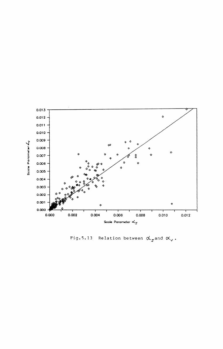
Sea In Po rometor (V

0.01}

0.012 -4

I0.011

10.010

10.009

0.000

0.007

0.006

0.005

0.004

0.00:5 1

0.®2 -4

0x1 -10.030

01130

O

O

0O0

0I I I I I0.G32 0.004 0.006 0.008 0.010 0.012

Fig.5.13

Scale Pororn-eter 0(3­

Relation between OCJ.and (XV .

The O(V values are found to be slightly higher. Thedeviation is more at the lower energy cases and less at thehigher energy conditions. In the lower energy cases theratio of CXV/<XJ range from 1 to 4 and in the higher energycases it is very close to 1. As indicated above, an isderived from the spectral densities in the high frequencyrange and CXV is derived from the total energy of the mea­sured spectrum. When the values are comparable at the high

energy conditions, higher values of av at low energy condi­tions can be possible due to two reasons - energy in the lowfrequency range of the spectrum being not proportional tothat in the high frequency range, based on which CXJ iscomputed, and/or the peak frequency being higher in thelower energy conditions. In the present data lower as wellas higher peak frequencies are present in both the condi­tions, though the number of occurrences are few. Hence, the

higher values of (xv observed at lower energy conditions maybe due to the first reason. But, it appears to be propor­tional at the high energy conditions. The shape parameter flof the Wallops spectrum is not related to <XJ or (Xv.Further, these parameters are not found dependent on otherspectral parameters.

131

5.5. CONCLUSIONS

The models which depend entirely on the peak frequencydo not show satisfactory representation of the data. Thus,the Jensen's modification to the Kitaigorodskii et al. modelwhich is entirely a function of frequency, fit :h1 a veryfew cases only and the total energy and peak energy densityare highly overestimated by this model. On the other hand,the models with total energy as one of the defining parame­ters exhibit better performance. Even the deep water Scottmodel and its modification by Weigel give better representa­tion than the Jensen's model. However, the dispersion rela­tionship proposed by Kitaigorodskii et al. is found to be astepping stone to derive shallow water spectral models.Some of the models derived based on this relation givesatisfactory results.

The TMA model gives better results and follow theobserved spectra in a large number of cases. This model is

particularly useful for high energy conditions where H8 isof the order of 1.4 m and above. On the average, the totalenergy is overestimated, especially in the low energy cases.However, the peak energy density is estimated correctly bythis model. This model is defined with 5 free parameters,and the derivation of these parameters requires the fullspectrum as input. But, in most practical cases, it is not

132

possible to define the full spectrum apriori to calibratethis model. Hence, a model with lesser number of freeparameters would be useful. If the average JONSWAP scaleand shape parameters along with Phillip's constant are usedin the TMA model, the number of free parameters can bereduced to 1. But, in that case the fit is very poor. Thetotal energy as well as the peak energy density are over­estimated. The application of the coefficient suggested byVincent (1984) improves the performance of this form, butnot to a level satisfactory for applications. This modifi­cation makes the total energy to be predicted correct to99%, but the peak energy density is overestimated. Thisform is capable of simulating the shallow water spectracorrectly for low energy and low peak period cases.Further, if the peak enhancement factor is made free, ie.,to be estimated from the measured spectrum, its application

can be extended to all Tp ranges for the low energyconditions. The total energy is slightly underestimated andthe peak energy density is overestimated by this form,especially in the high energy cases. fflue Wallops spectral

model finds its application in the cases with HS > 0.75 mwith T 5 10 s, to simulate the shallow water wave spectra.P

At higher T ranges (T 3 10 s), the total energy is over­P Pestimated and the peak energy density is underestimated bythis model. Hence, care should be taken while applying this

133

model to the cases with large peak periods, especially withhigh energy. The Scott model and its modification by Weigelestimate the total energy comparable txn the observed.However, the peak energy density is overestimated by thesemodels, especially at high energy cases. The modificationby Weigel improves the model slightly, but the coefficientsA and B need further modification to simulate the shallowwater spectra correctly for all conditions.

A new shallow water spectral model derived from the P-M

spectrum with the application of the dispersion relationshipproposed by Kitaigorodskii et al. (called PMK spectrum)presents a better fit to the data. Though this comes secondto the TMA model (which has 5 free parameters), the formerrequires only the 2 commonly available spectral parameters

(mo and fm) to define the spectrum. Hence, when the fullspectrum is not available to calibrate the 5-parameter TMAmodel, the 2-parameter PMK or Scott-Weigel spectral modelscan be used for practical applications.

134

CHAPTER 6

WAVE HEIGHT AND PERIOD DISTRIBUTION MODELS

The probability distributhmi of wave heights, periodsand their joint distribution are computed from the data andtheir characteristics are discussed. The observeddistributions are compared with different theoretical/empirical models and the ranges of applicability of thesemodels are examined.

6.1. DISTRIBUTION OF ZERO-CROSSING WAVE HEIGHTS

I

The distributions of individual zero-crossing waveheights are computed for each record at height intervals of0.2 m, typical examples of which are presented in Fig.6.1.The observed distributions exhibit multiple modes in some ofthe cases, especially in time high energy conditions. Thismay be due to the finite length of records considered forthe analysis. If- samples consisting of sufficiently largenumber of waves are considered, the insignificant modes maybe got eliminated. The short-term height distributionsderived from the data are compared with differenttheoretical/empirical models. The records corresponding to

10 ranges of Hsw at an interval of 0.25 m and 8 ranges of Tpat an interval of 1 s are combined and the resultant heightdistributions are also computed. The distributions thusobtained are also compared with the models and the resultsare presented in section 6.1.2.

135

Probability density

04f-]‘ : [T] mT2 = 7,60 3 061 11.30 sp = 0.42 + 0-44o2~

'1

oa

, , , , , , . , ac . . . . . . Ymo L0 20 ‘L0 44 O0 r0 10 30 *0041.38 m ‘ 1.24 m7.20 s o3~ 10.40 s1 0.49 , 0.51c>2* 021O-Ii O-H_10.0 . , O’-0 , j ,G0 20 30 +0 04: no 20 30 +00-4 041 1.61 m 1 1.55m045‘ 8.70 s 03* 9.60 s1 0.45 . 0.550-2" 0-2-11 '10-I« odwCLO , . . oo , . .0-0 2-0 3.0 4--O 0.0 1-0 2-0 5-0 4--O

Wave heighdwfl

Fig.6.1 Typical examples of observed height distribution.

6.1.1 Comparison of Short-Term Distributions with Models

The distribution of zero-crossing wave heights computedfrom each record are compared with the differenttheoretical/empirical models in this section. The usualpractice is to make visual comparisons to examine the fit ofa theory with the data. Typical examples of thedistributions predicted by the different models arepresented in Fig.6.2. A visual comparison is very difficultwhen the number of records and models considered are large,as in the present case. An alternative is to applystatistical tests of goodness of fit. A valid test that canbe applied here is the X? goodness of fit test. Hence, thefitness of each model to the data is evaluated using the‘X2test at 0.05 level of significance. The cases where thedifferent models fit the data are presented in Appendix-A.In order to apply this test, the data has to be grouped intobins of frequencies not less than 5. Hence, the tail of thedistribution has to be truncated by adding it to the nearestclass to make the frequency 3 5. In some cases, like thevery low height conditions, this may give unrealistic fitswith very few number of classes (like 2 or even 1sometimes). In such cases, visual comparison is made toevaluate the fitness. In addition to the application of theX? test, the cumulative probability densities of thestatistical height parameters, E, H and Hmax predicted bySW

136

Pm be btflty Ocnolty

Probablltty Ocnclty

0.26

0.24 -‘

0.22 ‘

0.20 "*

I0.18

0.16 -1

l0.14

0.12 -i

0.10 -‘

0.08 -<

0.06 ­

0.04 -4

0.02 -1

0.00

Wave Height (s)5 A 4+ 2 0 X 5 V 60.28

0.24 -1

0.22 -<

0.20 -<

0.18 -‘

0.12 -w

0.10 "‘

0.... J

0.06 -1

0.04 -4 °

0.02 -<

0.00

1:S:8:

10:

Wave Height (9)+ 7 o 8 A 9Observed, 2: Rayleigh, 3: Goda's, 4:G1uhovskii's, 6: Ibrageemov's, 7:Longuet-Higgins'(l975), 9:CNEXO and 11:

Weibull,Tayfun's,

CNEXO (modified) distributions.

Fig.6.2 Typical examples of height distributionpredicted by different models corres­ponding to an observed distribution.

Longuet-Hiqgins'(1983):

the models are also compared with the corresponding valuesobtained from the data. The results are discussed in sub­sections 6.1.1.1 through 6.1.1.8.

6.1.1.1. Rayleigh distribution

The Rayleigh model for the distribution.of individualwave heights (Eq.2.64) is found to fit the observed data in277 cases constituting 87.7% of the data set. The fit isfound to be equally good during the rough as well as thefair seasons. During the rough season this model is found tofit in 86.7% of the cases and during the fair season fit isobtained in 88.6% of the cases. Also, the fit is found to be

independant of Hsw and steepness (corresponding to thesignificant wave height and average zero-crossing period).

Fit is obtained at all Hsw and steepness ranges. However,it may be noted that values of steepness above 0.4 is veryfew in the data and the model is found not to fit in thosecases.

The cumulative probability densities of E, H and Hmaxsw

predicted by this model are presented against the observedvalues in Fig.6.3 (a-c). The probability densities of E areoverestimated in most of the cases and the predicted valuesare almost constant with lesser variations. On the average,the densities are higher by about 5%. The probability

137

densities of Hsw and H are closer to the observed, butmax

are slightly underestimated, the rate of which is about 2%,on the average.

The basic assumption in applying the Rayleighdistribution to wave heights is the narrow bandedness of thespectrum. In the present case the spectral width parametersranged widely indicating broad band spectra in a largenumber of cases. and the Rayleigh model is found to fit inthe entire range. Applicability of Rayleigh distributionbeyond the narrow band assumption has been observed by many

other researchers (Longuet-Higgins, 1975; Chakraborty andSnider, 1974; Dattatri et al., 1979).

6.1.1.2. Goda's model

The truncated Rayleigh distribution suggested by Goda(Eq.2.69) is found to fit zhu 227 cases, which constitutes71.8%. This model is found to have better representation ofthe rough weather data. During the rough season fit isobtained in 78.7% and during the fair season it fits in65.7% of the cases. This model also is found to beindependent of the Hsw, T spectral width and steepnessplvalues like the Rayleigh distribution.

The probability density of R is overestimated by thismodel also (Fig.6.4a). The deviations are larger than that

138

observed with Rayleigh. The average rate cflf overestimationis about 13%. As time statistical height parameter becomeslarger, the ratio of predicted to the observed probabilitybecomes lower and lower. When the P(fi) values are highly

overestimated, the values of P(HSw) are closer to theobserved (Fig.6.4b) and are higher by about 2% only. In thecase of P(H ) the values are very much comparable to themax

observed values (Fig.6.4c). In fact, they are underestimatedslightly, but the rate is much less than 1% only.

This model is a modification of the Rayleigh form toincorporate the breaking and broken components of wavespresent in the shallow waters. Thus, this model is expectedto have a better representation of the shallow water heightdistribution than the Rayleigh model. Since this is notachieved, the applicability of the 'breker index‘ (thisdetermines the shape of the distribution) to differentenvironmental conditions has to be examined. As this model

fits more of the rough weather data than the fair weatherones, it appears that the breaker index with the recommendedconstants (Eqs.2.7l and 2.72) wrongly estimates some of thenon-breaking cases as breaking. Hence, modification of theseconstants and validation of the breaker index is necessaryfor applications at different locations.

139

P R E D I C T E D

(a)

oz. 0+ 0%: 03

0.8 <

0-’? *

(b) ° ’

6

4LL.JJ1LL11J1L1J1LLl

O W

9m

Fig

Y V V V V V V Y V V V Y V V V V Y 7one "0

(5) ‘o-8« ,oo ’-< ‘S o 7!,.o o‘JO-6" .1 ° . 9' . ’ .. .

0-4" 0

0'2 1 I. V V 70,2 O.+ O-6 0'8‘'0 i" . 0 VV O0'31 . .. QO. OO‘\ O'* 9

:.~m§3.O-3-1 . 0'1

O-1"

0'6 Y I T V V ' ‘o.5 0'1 o-8 0 5 ‘OI-0 0.01 (c) , . .: . .09. Q 1'1 0 O 9%’ .O.¢ 09 l4 O ’.. .¢‘ 0 : 5 0-4 9 , . o

'1

0-911 .'1

1

0.8 V V V V i V 7 7 V V V V V V V Y 7 V008 0'8O B S E R V E D

.6.3 Plot of cumulativeprobability densities ofheight distribution pre­dicted by Rayleigh modelagainst observed:(a) H ;(b) Hsw 7 (C) Hmax°

Fig.6.4 Plot of cumulativeprobability densities ofheight distribution pre­dicted by Goda's modelagainst observed:(a) E ­<b>H ;<c)H 'sw max’

6.1.1.3. Weibull distribution

The Weibull disribution (Eq.2.73) is found to followthe data in 252 cases (77.7%). The fit is found to be betterduring the fair season with 86.7% of the data following thismodel. During the rough season it fits in 72% of the cases.Fit is observed in all the ranges of H T ,'steepness andsw' pspectral width ranges present in the data.

The probability densities cfifli are slightly over­estimated in this case also (Fig.6.5a). On the average, P(fi)is higher than the observed by about 3%. The predictedprobabilities of Hsw and H are lower than the observed inmax

most of the cases (Fig.6.5b-c). The average rate of under­estimation is about 4% for P(HSw) and 3% for P(HmaX).

Forristall (1978) obtained good fit with this model forthe data from storms in the Gulf of Mexico. The present datais found to deviate from this model more than the Rayleighdistribution. When Rayleigh is a function of 0th moment ofthe spectrum, Weibull is a function of the higher moments.That is,the frequency (or period) has more influence on thismodel compared to Rayleigh. The deviation of the presentdata set from this model may be an indication that theinfluence of period is less on the distribution of shallowwater waves, where the effect of refraction, shoaling, bott­om friction, etc. are more due to the gently sloping bottom.

140

6.1.1.4. Gluhovskii's model

The Gluhovskfi function (Eq.2.65) is found to sdmulatethe observed height distribution in 296 cases whichconstitute to 93.7% the total observations. The fit isequally good for both the seasons with a fit in 95.3% of thecases during the rough season and 92.2% during the fairseason. Fit to the data is obtained with this model in all

the observed ranges of Hsw, Tp, steepness and spectral widthin the data.

When predicted P(HSw) and P(H ) values are very closemax

to the observed, P(E) values are slightly overestimated by

this model also (Fig.6.6a-c). (mm the average P(fi) valuesare higher by about 2%. The ratio of predicted P([-lsw) tothe observed is 1, on the average, the deviation being lessthan 0.1%. P(HmaX) values predicted are lower by about 1%,on the average.

Gluhovskii distribution is reported txb follow theobserved height distributions closely for other parts ofthis coast (Saji, 1987). Unlike the other models, thismodel is depth dependent. From the close fit observed in themaximum number of cases, it may be inferred that thedistribution of wave heights in the shallow water is depthdependent.

141

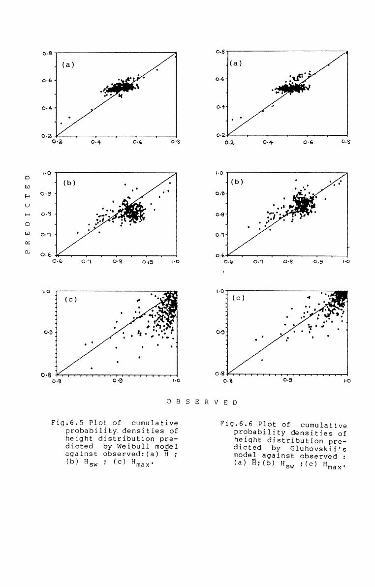
P R EI[) I C T E D

o-8 ‘4 (3) .. 00-6-4 °I’ \

~€-1 .09 ‘‘o-+<

J 00'2 1 Y 1 Y Icyz om; at 0%b0 -4 . 00. . 9crew ‘ .. 0T .00. . 04 .¢"'.o

1 . .'.o‘ Q 3 . 0OJ] 4 ’ . ‘0'6 1 1 Y Y V V Y0- 0'1 0'3 013 ‘0I-0 ‘3 ‘.0 ’4 1’3 . ~= o. .1‘ o 11 o o‘%-4 9 ’: .. 0O6: 3 °‘&°«o‘?}{1 . . 9 9 . '1I 0-J 9J o0.8 Y Y V V Y 7 Y Y V f‘ Y Y I Y I Y f'Y03 0% '0

Fig.6.5 Plot of

O8

'15.“. ‘0&4 ...-1 ."'O-4" ’

-1 . O

002 f 1 I v 1002 0'4 0'6 0'81-0 4 . . . . O.

O ...0'9.‘ ‘Q...0 O4 .... ~.’... ‘G0-8‘ . ’ * 0 I. .9‘ ’ 9''1 , . 0 .oni

0'6 1 I V Y 1 V vO-Co O-'1 0'8 0-9 "0

"O Q .(C) " . ’~4 . i1 . 90 .6 .‘i 0‘ . I1 . °. 0 04 . . R .0 ¢ 0 T4 . ’061 . ° ’ ° ° ‘J 0 O 9. . .31 .-4

4

0'8 Y r V T I r T V ffi V I v 1 v 1 I 1 100% 0.9 "OO B S Eli? V E D

cumulativeprobability densities ofheight distribution pre­dicted by Weibull modelagainst observed:(a) E ;(b) H ; (C) Hsw max’

Fig.6.6 Plot of cumulativeprobability densities ofheight distribution pre­dicted by Gluhovskii'smodel against observed ­<a> fi;<b> nsw ;(c) nmaxl

6.1.1.5. Ibrageemov's model

This model (Eq.2.67) is found to have very poorrepresentation of the observed height distribution. Fit isobtained only in 65 cases which constitute to 20.6% of thedata set. The representation by this model is nearly thesame during both the seasons. Fit is obtained in 22.7% and18.7% of the cases during the rough ENKl fair seasons,respectively. Although the applicability of this model ispoor, the cases where it fits the data fall in all ranges ofH TSW, 2, steepness and spectral width, indicating that thismodel is not dependant on these parameteres, eventhough wave

period is one of parameters used in defining this model.

The probability densities of fi, H and Hmax predictedsw'

by this model are ploded against the observed values inFig.6.7 (a-c). The probabilities of E, H and H aresw maxoverestimated in majority of the cases. P(fi) values arehigher, on the average, by about 4% enui P(HSw) values arehigher by about 11%. The predicted P(H are at themax)

maximum of the cumulative probability curve in most of thecases.

This model is a modification of the Gluhovskii's byincorporating period as an additional parameter. However,it fails to simulate the observed height distribution inmost of the cases, where the Gluhovskii's function estimates

142

the values more closely with the observed. This indicatesagain that the period is not a controlling parameter for thedistribution of wave heights in shallow waters, whencompared to the depth. Reports of validation of this modelelsewhere is not seen in the literature.

6.1.1.6. Tayfun's model

The Tayfun's function for wave heights (Eq.2.77) isalso found to be very poor in simulating the shallow waterdistribution of individual wave heights. With the presentdata it fits only in 57 cases (18%). However, this model ismore suitable for the rough sea conditions. The cases wherethis model fits the data are the cases of the rough weatherconditions. During May-September this model is found tofollow the data in 36.7% of the cases and the fit is found

to be better for the higher ranges of Hsw, steepness andspectral width and for the lower ranges of T2. That is,thismodel may be applicable to the conditions of high, steepwaves, such as that occur during the peak monsoon.

The probability densities of E, H and Hmax predictedsw

by this model is presented in Fig.6.8 (a-c). Theprobabilities of E are estimated in a large range, most ofwhich are lower than the observed. It does not show anycorrelathmn with the observed, except zhi a few cases.

143

PREDICTED

40.8 -{ ) .'.o Q. . O9‘ .1, O0. 0. .0-61 9

Q‘ P04* ° %’r‘.. V0.2 , , r _v_ v __0.2 O°4- 0-6 08

"O V 0 ’O

‘ (b)081

‘i

0O8 1 ,-4 O 90-71

0'6 1 I I I r 1 Vo£> o'7 c>8 <39 *0

V01 .3 J 3 Q5 . . W.4 Q °. .'1I 9d 04 0

ca}I

098? V - V T V V U ‘U I I U I I Y ' ' V V Y T0-8 0-3. \-0

Fig.6.? Plot of

O80‘(a) .O-6" ” 9 ° ‘" I Q .0o . " 9.0'41 0 ’. ‘"6 O

90'21 0.0‘ 009. o" 9 0 9099 OO. O , 1, 3:, ::::a,‘: e j— _o-2 ' o-4- 0-6 0-8

no,Mb) . ' .‘ § '0 .‘ 40'91 8O1 ° 09 Oo8~ 3 ‘» « ~33’1

::~gon T . Q .’9'9Q 0 .9-4 . .09 .O at Q .06 V V V V 1 i! rO 6 O '1 0-8 0 9 I 0

I-Oj (C) . , .’v-1 ' §’3 :0 ’ -, /+ o5°.o 9‘i 9 6 Q . . {-1 ’ °’0 . ,0-3" 9 . y-4 . .. 01 . .:,4 01 O 9 02 . ,: ’ ‘9

0'8 V 1 Y I V V v r 1 y 1 7 y , Y Y Y , ,0-8 0-3 I-OOBSERVED

cumulativeprobability densities ofheight distribution pre­dicted by Ibrageemov'smode} against observed :(a) H:(b) H ;(c) HSW max‘

Fig.6.8 Plot of cumulativeprobability densities ofheight distribution pre­dicted by Tayfun's modelagainst observed:(a) H ;(b) H ; (C) HSW max’

P(HSw) and P(HmaX) estimated by this model are closer to theobserved in most of the cases. But the range is wider and afew values are very low compared to the observed. On theaverage, the values are lower by about 10% in the case ofP(HSw) and 3% in the case of P(HmaX).

The Tayfun's distribution function is developed withthe observation that the crests and troughs of the oceanwaves do not occur at the same time and the envelope of thewaves will change during the half wave period, if the spec­trum is narrow (Tayfun, 1983b). If the wave is high, it islikely that when the crest is near an extreme of the enve­lope the associated trough will have a smaller amplitude, sothat the wave height will be less than twice the amplitude(Forristall, 1984). In such cases, it is hypothesised thatit is the wave envelope that follow the Rayleigh distribu­tion rather than the waves themselves. In the present casethis model is found to simulate the observed distributions

corresponding to the rough weather conditions. During therough season the waves observed here are of higher energyassociated with comparatively lower periods and spectralwidths (Ch.3 & 4). Thus the hypothesis of wave envelopefollowing the Rayleigh distribution (rather than the waveheights) appears to be true when the waves are high and thespectrmn is narrow. However, the failure cfif this model inthe cases of spectrum with 1ower energy andlorger width,

144

where the wave heights are found to follow the Rayleighdistribution, indicates that the envelope approach is notvalid to such cases. Hence, it is suggested that this modelmy be used to simulate the wave height distribution inshallow waters during high wave activity or stormconditions.

6.1.1.7. Longuest-Higgins‘ models

The distribution of heights and periods suggested byLonguet-Higgins zhi 1957 was recapitulated .h1 1975. Byintegrating the joint probability density function given inEq.(2.90), the function for the distribution of heights isobtained as Rayleighean. This was modified by him later(Eq.2.91) to incorporate the effects of non-linearity andfinite band width (Longuet-Higgins, 1980 and 1983). Theprobability density function of heights obtained from theabove 2 models (Longuet—Higgins, 1975 and 1983), by integra­

ting the joint probability functions with respect to period,are compared with the observed height distributions. Anexamination of the performance of these models may throwmore light into the quantum of the effects of non­linearities on the distribution of wave heights in theshallow water conditions.

The first model (Longuet-Higgins, 1975) fit in 288cases which constitute to 91.1%. The modified form

145

(Longuet-Higgins, 1983) fits almost equally well, but lessby a few number of cases. It fits in 280 cases which is88.6%. During the rough as well as the fair seasons boththe models fit nearly equally, the modified form showingslightly better fit during the rough season. During therough season both the forms fit in 90.7% of the cases eachand during the fair season the first form fits in 91.6% andthe modified form fits in 86.7%. In all the ranges of H sw'

Tp, steepness and spectral width present in the data, boththe forms are found to fit almost equally.

The probability densities of El predicted by both themodels are found to be closer to the observed values, butare slightly underestimated by the first form andoverestimated by the modified form (Fig.6.9a-b). On theaverage, when P(fi) values are underestimated by about 6% bythe first form, it is overestimated by about 5% by themodified form. The values of P(HSw) are also estimated in asimilar manner by both the forms, the modified form being inbetter agreement with the observed (Fig.6.9c-d). On theaverage, the first form underestimates the values by about5% and the values predicted by the modified form deviates byless than 0.1% only. Also, the scatter is minimum in thecase of the modified form. The values of P(H ) aremax

underestimated by both the forms, but the deviations are

146

less with the modified form (Fig.6.9e-f). The predictedvalues, on the average, are lower by 13% in the case of thefirst and about 1% in the case of the modified forms. Thatis, the probability density of the lower ranges of heightsare simulated equally correctly by both the forms andheights of the order of Hsw and more, where the effects ofnon-linearities are more pronounced, are simulated morecorrectly by the modified form. As the probabilitydensities of the larger height ranges are of importance inpractical applications, the modified form of thedistribution function may be more suitable.

6.1.1.8. CNBXO models

Intergrating the joint probability distributionfunction for heights and periods suggested by the group ofCNBXO (Eq.2.93) with respect to period, the distributionfunction for heights is obtained. The probability densityfunction for individual wave heights thus derived is nearlythe Rayleighean when spectral width is not large. Goda(1978) observed that the rank correlation r(H,T) would be a

better parameter rather than ew in this model. The relationis thus modified by substituting r(H,T) in place of ew. Theprobability distributions of heights computed using thesefunctions (original and modified forms) are compared withthe observed height distributions.

147

P R B D I C T E D

Longuet-Higgins'(1975)0-3

4

aJ < >V

O . .oe+ .,,a9 Q~ I9 o .00.4-4 0 9

0

0'2 7 W V T Y(5.2 0%.. 0.6 0-8I00

7

'1

o.9­

'1

4 Q .91 00'6 r r t v fl 7<35 08 no|°O ‘ oQ .0’4 51 v '9 o '9 ‘-I . .. .‘ ° 0 o.“ 3.?0.93 . , ° °~‘ O3 O Q . . O ‘0-4 . ’ O QI 9

'4

0°81 1 v v v .7 v v V I Y I V V V V V V V009 "O

Longuet-Higgins'(1983)O-31 ‘1 . 0. OO....c.O0.61 09O O.-I O ‘ ‘‘ . 0 ° 0 P

O~4»“

0

0'2 Y V V T02 04» oz 09I-0

0-8‘ 3wi

'1

09.6 V + Y 1 I V I“O5 08 V01'03 ( f)

"1-I O.4 Q 0J O-I-1 ’ °O-9: 0 ' , '-J

'1~ 0I

'1

0.8 Y’? Y I V V V I V V V Y 1 t 1 1 [ r0.8 0'9 \'OO B S E R V E D

Fig.6.9 Plot of cumulative probability densities of heightdistribution predicted by Longuet-Higgins 1975 and1983 models against measured respectively;(a) & (b)'fi; (c) H ° (e) & (f) HSW ’ max‘

On comparison of the distributions predicted by theabove 2 forms, it is found that both the forms do not givesatisfactory results. They fit in very few cases only.However, the performance of the modified form is better thanthe original. When the original form fits in 116 caseswhich contribute to 36.7% of the data, the modified formfits in 178 cases (56.3%). On a closer examination, the fitis found to be better during the rough season for both theforms. The original form fits in 43.3% of the cases duringthis season and 30.7% during the fair season. fflna fit bythe modified form during the rough and fair seasons are 60and 53% respectively.

Both the forms give fit in all the ranges of Hsw, Tp,spectral width and steepness. However, the fit is found tobe better at higher steepness ranges by the original form.The modified form give better representathwi at the lowersteepness as well.

The probability densities of § predicted by both theforms are higher than the observed in all the cases, exceptin a very few ones (Fig.6.l0a-b). On the average, thevalues are overestimated by about 22% by the original formand about 18% by the modified form. The P(H values aresw)

also overestimated by these models, but are comparativelymore closer to the observed (Fig.6.10c-d). On the average,

148

P(Hsw) values are higher by about 4% in the case of theoriginal form and about 3% in the case of the modified form.However, the values of P(H are predicted more correctlymax)

by these models (Fig.6.lOe-f). The average deviation fromthe observed, in both the cases are much less than 1% only.That is, though the modification of the model with r(H,T) in

place of ew improves the model slightly, it does not bringit to the desired level for applications in shallow waters.

6.1.2. Comparison of Observed Distributions in the HS‘-TpRanges with Models

The different models considered above for comparisonwith the distribution of wave heights in individual recordsare also compared with the distribution of heights obtained

by grouping the different records in Hsw intervals of 0.25 mand period intervals of 1 sq Upon grouping 13 classes donot follow any of the models, due to the presence ofmultiple modes in the distribution. Hence, these cases arenot considered for the comparison. A few cases withmultiple modes are not excluded, since one or the other ofthe models fit in those cases.

The observed distributions are generally positivelyskewed and the coefficient of skewness are predominantly inthe range 0.1-0.8 with an average around 0.4. The dominantkurtosis values are in the range 2-4 with the average

149

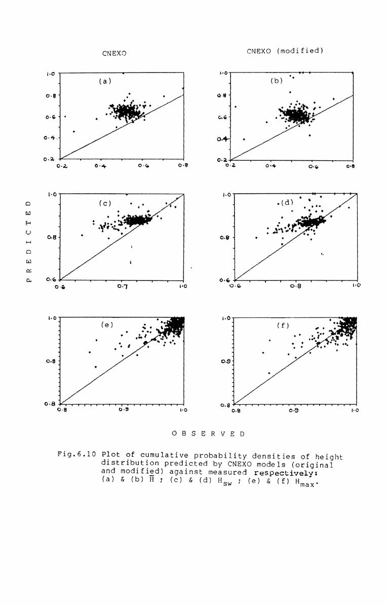
P R E D I C T E D

CNEXO (modified)CNEXO1.0 v no-1 1T008‘ .’ O 1+O I ,1 :0 Y?’ we

90'6 1 ‘ ..’ .7 ° 70'4-" Q‘ w0.2 f ' 7 7 0'2 1 1 1 T 10.; C-4, 0'“ 0'8 O’; 09¢ 008L0 v »o e, * ~*’

6'1 . . ’ ’ . " 9 to .o o v ' o 01 . 0’ ~ Q. -1 . QC .9_‘ 9 ;0o. _‘ : '9‘ fo“‘. I Jqoxto . .:08'‘ 0 O-9 " O 0 ..O.. ‘ 4-_ L-1 ‘ 1T -10'6 V V V 1 1 0'6 1 I r 1 1 W r05 01 so «me c>8 *0‘‘o.‘ "O .D ‘ (f) 0’ 0 Z.I 1 . . . O:..‘ O: 1 .0 ’ 0° .‘ ..‘ ‘4 '4 Q .‘1 " . 0 .0-31 0.9-‘I 1 .1 '1-J -4I 1-4 -J

_ *0'8 TYYFTTTYYf‘rv1rvrvW1 0.8-‘YYYVVVTTFYTVYfVUVYY03 O3 vo Q3 oe hoO B S E R V E D

Fig.6.lO Plot of cumulative probability densities of heightdistribution predicted by CNEXO models (originaland modified) against measured respectively:(a)&(b)H;(c)&(d)H ;(e)&(f)HSW max‘

slightly less than 3, which is the value for a normaldistribution. This marked skewness and the lower values of

kurtosis indicate the degree of deviation of thedistribution from the normal. However, the fit cnr non-fitof models are not found to be dependent on values ofskewness or kurtosis.

The average skewness and kurtosis of the Gluhovskii'sdistribution is in good agreement with that obtained fromthe data. All other models show higher skewness and kurto­sis, except Ibrageemov's, which has values lower than thedata. Gluhovskii's model fit in all ranges of skewness andkurtosis present in the data. The Longuet-Higgins’ 1975model and Goda's model show a fit in the lower ranges ofskewness only. They do not fit in any case corresponding tothe higher values of kurtosis also. All the other modelshas a few cases of their fit in the lower ranges of skewnessand kurtosis, with the modified form of CNEXO fitting in thevery low ranges only.

The cases where the different models fit the data arepresented in Table 6.1. Gluhovskii's and modified Longuet­Higgins models give better fit with the data. They followthe data in about 80.5% of the cases. Rayleigh and Weibullfuntions follow the data almost identically and they fit in46.3% each. Fit by Tayfun's model in 34.1%, Goda's in 31.7%,

150

Tnb10 6.] Pit of Different Height Distribution Hodnlnto Data in H33-Tp Rangesqu--oc--—-—o.¢——¢—-p-———-o-:——n—-——-—:¢¢:—_-¢¢-—q--o———o¢——--cu-——o-.-cc-p--—

Nu H,c(m) Tp(s1 Aco C1 L1 L2 81 C1 ufi 1“ Fy "1 P21 0.00-0.25 5 - 6 32 0.00-0.25 6 - 7 3 X K x3 0.00-0.25 9 -10 3 I I x4 0.00-0.25 10 -11 11 x5 0.00-0.25 12 -13 16 Y6 0.00-0.25 15 -16 4 x x7 0.25-0.50 6 - 7 4 x x x r I x xR 0.25-0.50 8 - 9 4 x x x I I9 0.25-0.50 -9 -10 8 x x x10 0.25-0.50 10 -11 13 I

11 0.25-0.50 12 -13 4212 0.25-0.50 15 -16 12 x x I I13 0.50-0.75 5 - 6 2 x x I I14 0.50-0.75 6 - 7 315 0.50-0.75 8 - 9 216 0.50-0.75 9 -10 9 x 117 0.50-0.75 10 -11 8 x I18 0.50-0.75 12 -13 4119 0.50-0.75 15 -16 10 x Y20 0.75-1.00 5 - 6 1 x V I I I I I21 0.75-1.00 6 - 7 1 x x I22 0.75-1.00 7 - 8 1 X V V K V I21 0.75-1.00 8 - 9 224 0.75-1.00 9 -10 5 x x25 0.75-1.00 10 -11 3 x Y26 0.75-1.00 12 -13 12 x v27 0.75-1.00 15 -16 220 1.00-1.25 6 - 7 329 1.00-1.25 8 - 9 6 x30 1.00-1.25 9 -10 6 x x x71 1.00-1.25 10 -11 7 x x x x I72 1.00-1.25 12 -13 5 x x x x I13 1.00-1.25 15 -16 1 x x x 7 x I I14 1.25-1.50 6 - 7 3 x x15 1.25-1.50 7 - 8 336 1.25-1.50 8 - 9 12 x37 1.25-1.50 9 -10 9 x I x38 1.25-1.50 10 -11 5 x39 1.25-1.50 15 -16 1 x x x V x v I K40 1.50-1.75 8 - 9 4 x x I41 1.50-1.75 9 -10 442 1.50-1.75 10 -11 343 1.50-1.75 12 -13 1 x x x x K x (44 1.50-1.75 19 -20 1 x x x x x x < X I45 1.75-2.00 7 - 8 1 x x X x I K46 1.75-2.00 8 - 9 1 x x x x I I I v47 1.75-2.00 9 -10 4 x x x x x x48 1.75-2.00 10 -11 3 X x x X I49 1.75-2.00 12 -13 1 x x x50 2.00-2.25 8 - 9 1 X Y. Y X X :I51 2.00-2.25 9 -10 3 V X x x x x52 2.25-2.50 8 - 9 251 2.25-2.50 10 -11 4 x x <AVG: Numhnr of records usofi for avoraqinqC1: C1uhovskii, L1, L2: Lcnguet-Hiddins 1975 AH4 1921P1: Rnylninh, Cd: Gofia, Nb: Weibull, Ib: Tbf3G°“”fiVTy: Tayfnn, C1, C2: CHER? nridinal nn4 ~o4iFin1

Ibrageemov's and modified CNEXO in 11.6% each and originalCNEXO in 7.3% of the cases are obtained.

In the lower height range of O-0.25 m the fit is verypoor for most of the models (Table 6.1). Tayfun's functiongives the best representation in this range followed byLonguet-Higgins’ 1975 model. Weibull distribution andLonguet-Higgins‘ modified form are found to fit in a veryfew cases. In other ranges, Gluhovskii's and Longuet­Higgins‘ modified forms follow the observed distribution ina large number of cases. They fit the data in all the rangesof Hsw equally well, except the lowest (0-0.25 m). Weibulland Tayfun's models represent the data better in the higherranges of Hsw. Ibrageemov's and the CNEXO models fail tofit the data in the lower as well as the higher Hsw ranges.Rayleigh and Goda functions represent all the height ranges,except in the lowest (O-0.25 m), though not as good asGluhovskii's and modified Longuet-Higgins’ models.

When the fit is examined in relation to the Tp values,almost all the models fit equally in all the ranges of TD.Gluhovskii's model give the best fit, followed by the modi­fied Longuet-Higgins‘. This is followed by the 1975-form ofLonguet-Higgins . All these 3 models show better representa­tion in the T range 9-10 s. Rayleigh and Goda's functionsP

show best representation in the lower T ranges of 7-8 s.P

151

The probability densities of the different heightparametes predicted by the models are identical to thatobserved in Sec.6.l. Gluhovskii's model predicts the valuesnearest to the observed. The maximum deviation is less than

2% only. P(§) and P(Hsw) values are overestimated by about1% and 1.5% and P(H is predicted correctly by thismax)

model. The modified form of Longuet-Higgins also predictsthe probability densities close to the observed values. Themaximum deviation is in the case of P(§) and are on theaverage overestimated by about 3%. P(H is overestimatedSW)

by about 1% and P(H is overestimated by less than 1% bymax)

this model. The deviations of the predicted values of theseheight parameters from the observed are found to be morewith the other models. The P(§) values are overestimated byabout 4, 5 and 6% respectively by Weibull, Rayleigh's andIbrageemov's functions. Goda's and the two forms of CNEXO's

models highly overestimate the values, in the range 12-20%,whereas Tayfun function underestimates them by about 33%.

P(Hsw) values simulated by Rayleigh is in goodagreement with the observed. When Goda's and CNEXO's models

overestimate the values tnr 4-6%, Weibull and Lbnguet­Higgins‘ first form underestimate them by about 2-3%. The

P(HSw) values predicted by Ibrageemov's and Tayfun's modelsshow maximum deviation, Ibrageemov's overestimating them by

152

about 13% and Tayfun's underestimating by about 11%.However, P(H values are predicted closely with themax)

observed by all the models. When the values estimated byGoda's and both the CNEXO models are in close agreement with

the observed, Rayleigh model underestimate them by about 1%and Weibull, Tayfun's and [mmguet-Higgins’ first formestimate the values lower by about 2% and Ibrageemov's modeloverestimates them at this rate.

On a closer examination of the different probabilitydensities predicted by the models, it can be seen that P(fi)is predicted most correctly by Gluhovskii's model withminimum scatter. P(H is predicted closest to thesw)

observed by Rayleigh followed by Longuet-Higgins‘ modifiedform and Gluhovskii's model. Weibull and Longuet-Higgins‘first form also predict the values comparable to theobserved, but are slightly underestimated. P(H valuesmax)

are estimated nearer to the observed by all the models,except Ibrageemov's which always overestimates the values.The values predicted by Gluhovskii's model is found to beclosest to the observed with minimum scatter followed by themodified form of Longuet-Higgins‘.

The depth controlled function of Gluhovskii simulatesthe probability densities of all the statistical heightparameters, whereas the other models overestimate them in

153

the lower height ranges. This indicates also that thedistribution of wave heights in shallow waters is alwaysdepth dependant.

6.2. DISTRIBUTION OF ZERO-CROSSING WAVE PERIODS

The distributions of individual zero-crossing waveperiods are computed from each record at 1 s interval.Typical examples of tflua observed short-term perioddistributions aux: presented ix: Fig.6.ll. Multi-modeddistributions are observed in a large number of cases. Thereason for this may be the same as in the case of heightdistributions. The observed distributions are compared withthe different theoretical/ empirical models. The perioddistributions are also computed from the records grouped

according to Hsw and Tp ranges, as done in the case ofheight distribution (section 6.1.2). They are also comparedwith the different models and the observations are presentedin sub-section 6.2.2.

6.2.1. Comparison of Short-Term Distributions with Models

The distribution of zero-crossing periods obtained fromeach record are compared with the different models in thissection. Typical examples of the period distributions predi­cted by the models are presented in Fig.6.l2. In this casealso, it is practically very difficult to do visual compari­

154

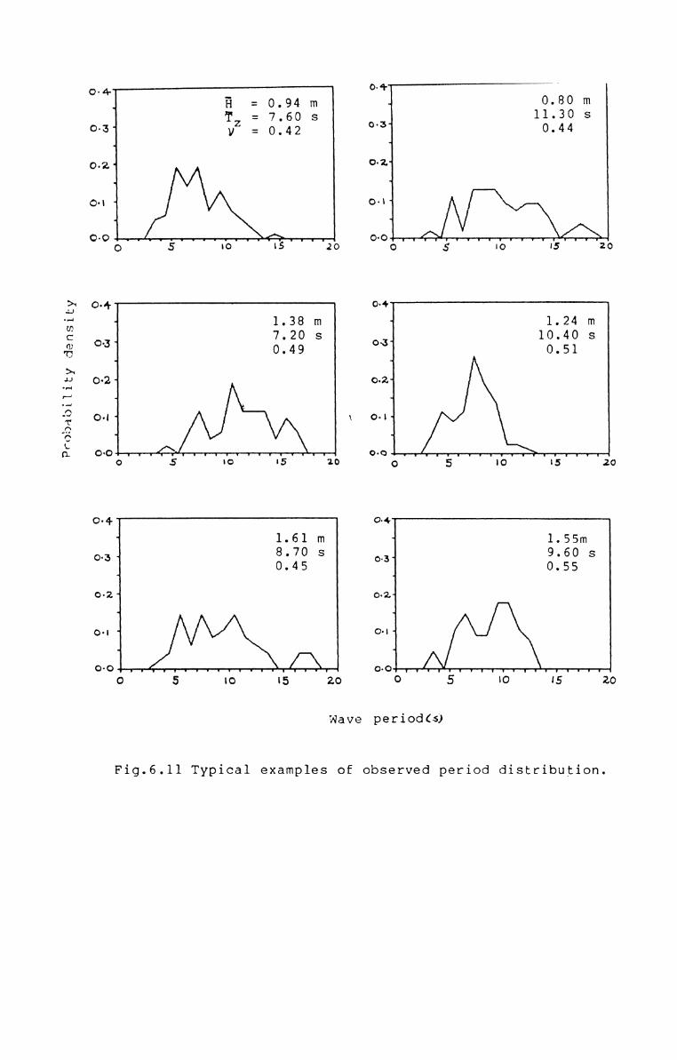
Probability density

0'4‘ 0'4‘ 7‘ ‘H = m '4 mT2 = 7,60 s 4 11.30 S0'3‘ V : 0.3* 40,2-4 C-211 '4O\ " O 1'14 '10'0 xv’ v v r v % V r v r v v v v r 1 r tr 0'0 11 TU VYTV 1 v V V777 v vvrvo 5 to I5 20 o 5 so :5 2o00* 0'4« 1.38 m 1 1.24 m7.20 s 10.40 s0- -33* 0.49 ° 1 0.51'1 10%‘ oz*« 1O!‘ \ O I-«I ‘10'0 T Y v{\r V V V 1 V v % 1 V V Y v vv r y ; g y & r y y V 1y‘ 1 "'f'o 5 so :5 20 o 5 no :5 200-4 04‘ 1.61 m * 1.55m8.70 S 9 60 80-31 (3.3-< '0.45 0.5502'‘ 0-2.‘* 1O-I O°|‘0'0 v v v Y’“Y v w v v r r 1 v v W 1 v r 0'0 T V r r r I 1 1‘1 Y 1 TY fr 1 1 v vo 5 to $5 20 0 5 IO 15 20

Wave periodcfi

Fig.6.11 Typical examples of observed period distribution.

son of the observed distribution with the models, since thenumber of observed distribution as well as the number ofmodels considered are large. The only satisfactory testthat can be applied in this case is again the‘X? goodness offit test. Hence, the fitness of the different models isevaluated using the‘X? test at the 0.05 level of significan­ce. The cases where the models fit the data are presented inAppendix-A. In addition, the cumulative probability densi­

ties of TC, T2 and TS in the observed distributions are alsocompared with the corresponding values predicted by thedifferent models. The results are discussed in sub-sections6.2.1.1 through 6.2.1.5.

6.2.1.1. Rayleigh models

The Rayleigh distribution for wave periods suggested by

Bretschneider fEq.2.69) is found to fit the data in 171cases constituting 54.1% of the cases. This model fits morecases during the rough season than the fair season. Duringthe rough season it follows the data in 62.7% and during thefair season it follows in 46.4% of the cases. However, this

model is found to fit equally in all ranges of Hsw, T2,steepness and spectral width.

The cumulative probability densities of TC, T and T82

predicted by this model are closer to the observed values(Fig.6.13a-c). The range of values are maximum for P(Tz) and

155

Pro bo bmty Oonflty

Probobmty Denalty

0.30

0.28

0.26

0.24

0.22

02040.18

0.15 1

0.14 -+

0.12

0.10

0.08

0.06

0.04

0.02

0.00

0.30

0.28

0.26

0.24

0.22

0.20

0.18

0.16

0.14

0.12

0.10

0.08

0.06

0.04

0.02

0.00

‘—_ “Va,-‘%s——%__I r I r’0 2 4 6 8 10 12 14 16 18Wave Period (9)——— 1 + 2 0 3 A 4 X 5

1

1

1

1 .3 5 7 9Wave Period (9)—— 1 + 2 O -3

1: Observed, 2:and 5: CNEXO

CNEIXORayleigh, 3:(modified)

Tayfun's, 4:distributions.

Fig.6.12 Typical examples of period distributionspredicted by different models correspondingto an observed distribution.

least for P(Tc). The P(TC) values are almost constant in avery narrow range and on the average are lower by about 4%

than the observed. The predicted values of P(Tz) are alsonearly constant, but with a wider range. On the averageP(Tz) predicted by this model is lower than the observed by5%. The values of P(Ts) are in good agreement with theobserved, but with some scatter. On the average, thepredicted values are higher by aflxnn: 2%. That is, theforward phase of the probability distribution of periods(the lower period ranges) are more flattened by this model,but can be used to estimate the cumulative probabilities of

the higher periods (> T2).

The Rayleigh model is adopted to represent the short­term distribution cu? wave periods tn! Longuet-Higgins,Gluhovskii and Tayfun while deriving their equations for thejoint distribution of wave heights and periods. The perioddistributions obtained from Eqs.(2.89-2.91) are Rayleighean.The distribution of periods obtained from Gluhovskii's andLonguet-Higgins's models are the same as the Rayleighdistribution discussed above, with identical fit with thedata. So, a discussion of the distributions obtained fromthese models are not presented here. However, Tayfun'smodel is a modification of the Rayleigh form by normalisingthe relation to have a unit area over the restricted

156

interval (-1/y , +1/U ) of the normalised period. Thedistribution of periods predicted by the Tayfun's model isdiscussed in the following section.

6.2.1.2. Tayfun's model

Tayfun's model for the distribution of individual waveperiods, derived from his model for the joint distributionof heights and periods (Eq.2.98), is found to fit in a largenumber of cases. Fit is obtained in 219 cases whichconstitute to 69.3% of the data. The fit is found to bebetter during the months of monsoonal wave climate. DuringMay-September fit is obtained in 80.7% of the cases andduring October-April, when fair weather conditions prevail,this model fits the data in 59% of the cases. The model is

found to fit the data in all the ranges of Hsw, Tz,steepness anui spectral width ranges. However, the fit ix:the case of lowest steepness values are not as good as ix:the other ranges.

The probability densities of TC, T and Ts pmedictedZ:

by this model also sflunv characteristics almost similar tothat observed in the case of Rayleigh and Gluhovskii models(Fig.6.l4a—c). Though the ranges of values are comparativelymore with this model they are distributed around theobserved values almost equally on the higher and lowersides. On the average, the values are in agreement with the

157

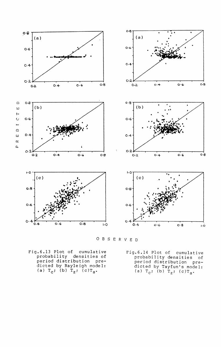
PREDICTED

90‘(a)

9osi 'I O 9.. J .9

OAW

0'2 7 Y ' V Yoz 04- 04> O8O-8

(b)1C-6" 9

9

"i .9 6 .. . ’ 9 .9.9 S’. /3O-4-< 9' ". s9 0£O-Z v v ' ' '0-2 0'4’ 0'6 C‘8

PO’W (c) t.9

0 } of 909. Q9. .O-8 " .§O«’.O . Q5 0 O O

1 ~.:§¢' %.O.‘ 9 0do 96 °0.6-1 9 :f‘ ‘y.’ ‘ °Q 9 '0, 97° ‘/9-1 .?..9 .9 '9. ..O. {V I V Y T4,0-+ 0'6 0'8 10

9 . 9 V '94 (a) ' 90 99 9: , .0.6-I . '... ‘.0 .. ' .. .

9Qw o’ ‘* M.0+4 '

'1

0'2; 7 V V ' Y .0.2, o-4- O-6 0-3

O-8 (b) ' '° °J Q 0. .9 . ’‘9

0.61 9 O .\ ‘$9.9.’ . ‘' O‘. Q. ' O. 0q . , 0. ‘9 99 9 X.O . . ‘o4? f " H‘O

-4

0'2 r V V V0 2 0.4. O 6 0‘8

no u ._ (C) ., .°.. .99-4 0 z‘ .9 . '0'8 ’ 9 9 9

. .'.?Q. . 5O,+ ‘. . O X Q9 o .9 . .9

0.64 Vqo : .0‘ «if. .‘ .3 : 9 g4 .9 ft. 9 39, ‘, 90.4- Y . r V r _04- 0-6 0-8 I-OOBSERVED

Fig.6.l3 Plot of cumulativeprobability densities ofperiod distribution pre­dicted by Rayleigh model:(a) TC; <b> T2; <c>TS.

Fig.6.l4 Plot of cumulativeprobability densities ofperiod distribution pre­dicted by Tayfun's model:(a) TC; (b) T2; (c)TS.

observed as shown by the regression analysis. The predicted

values of P(Tc), P(Tz) and P(Ts) deviate from the observedby less than 1% only. The underestimation of the lowerperiod statistics by the Gaussian normal models and theequally good fit obtained for all the statistical periodswith this model shows that the shallow water. wave periodsare not distributed Gaussian normal.

6.2.1.3. CNEXO models

The CNEXO disributions for periods are obtained byintegrating E2q.2.94 and the equation obtained by modifyingthis equation by replacing the spectral width parameter withr(H,T), with respect to height. The original form and itsmodification are found to be very poor in representing theshallow water wave period distribution. Altogether, theoriginal model fit in 92 cases and the modified form in only8 cases constituting to 29.1% and 2.5% respectively. Amongthe cases where fits are obtained, the original form followsthe rough season waves and the modified form follows thefair season ones. The original form fit in 35.3% of thecases during the rough season and 23.5% during the fairseason. The modified form fit in less tfluum 1% during therough season and 4.2% during the fair season. The caseswhere the original form fit, fall in all ranges of Hsw, Tz,steepness and spectral width. However, sufficiently large

158

number of cases which fit the data are not available toassess the fit at different height, period or spectral widthranges. The very few cases where the modified form fit thedata are in the low height and steepness ranges with higherperiod and spectral width.

The probability densities of Tc, T and Ts are highlyZ:

overestimated by both forms (Fig.6.l5a-f). The rate ofoverestimation is more for lower period parameters andlesser for higher period parameters. The average rate ofoverestimation of P(TC) and P(Tz) by the original form are21% each and that by the modified form are 15% and 10%

respectively. Similarly the values of P(TS) areoverestimated by about 8% and 9% respectively by theoriginal and modified forms.

6.2.2. Comparision of Short-Term Distributions in HS"-TpRanges with Models

The distribution of periods are computed with the data

grouped into different Hsw and 1? ranges, as done for theP

distribution of heights. The multiple modes observed in theperiod distribution computed from individual records aremore pronounced now, and almost all show major secondarymodes. As a result, the X? values become very high andpractically no fit is obtained with any of the models in

159

P R E D I C T E D

CNEXO (modified)CNEXOo.8 0-8(a) , ‘ (bi *O 4 f* ‘.0 9 , ’ 0 0‘owC)_b., . ‘. 0. 0 0.6-1 . ‘.0 “ ..O ... .'..o ‘ "5 .. . . 0 9T 1 O Q .9 ‘ 9 ' .o.q.J Oo4-'* 0-1 '10'2 1 v V 1 V ' ‘ V Y02 0+ as 08 o4 04- 06 930-8 o _./ 3(C? . (d)-4 . . 4 0 .'0‘? ‘.. ‘.4’ \ ' 0.0061 V 6 ' . O‘6 : 0.61 .09 £. ‘Q . ',9 O ' Q3‘ '‘ 3 ‘ '* . . ‘ : 99 5.. ‘ 1.‘ .. 9.1 Qty .0.4. O'++ . Q . O-4 4 9 . ‘‘I 00'1 7 7 r " .9 .0.; 0.4 0.6 O.” ’ I 1 I 1 10-2. 0'4 0 Co 0.9|'O "O4 _* °oa¥ O3,1 q

00"" 0.6.. .-1. . < o. 00+ V ‘ I Y 0'4 Y 1 I Y°'4— 0-6 0-8 I o 0-4 0 g 0 9 Lo0 B S E R V E D

Fig.6.15 Plot of cumulative probabilit d ° °of period distribution predicied Egséééigmodels (Original and modified respectively;(a) & (b) Tc; (c)&(d) T2; (e)&(f) TS_

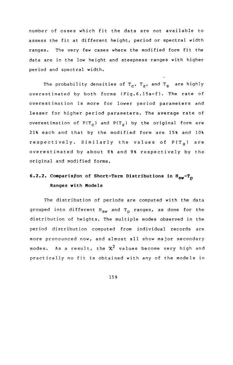
number of cases which fit the data are not available toassess the fit at different height, period or spectral widthranges. The very few cases where the modified form fit thedata are in the low height and steepness ranges with higherperiod and spectral width.

The probability densities of TC, T and T5 are highlyZ:

overestimated by both forms (Fig.6.l5a-f). The rate ofoverestimation is more for lower period parameters andlesser for higher period parameters. The average rate ofoverestimation of P(TC) and P(Tz) by the original form are21% each and that by the modified form are 15% and 10%

respectively. Similarly the values of P(TS) areoverestimated by about 8% and 9% respectively by theoriginal and modified forms.

6.2.2. Comparision of Short-Term Distributions in HS“-TpRanges with Models

The distribution of periods are computed with the data

grouped into different Hsw and 1? ranges, as done for theP

distribution of heights. The multiple modes observed in theperiod distribution computed from individual records aremore pronounced now, and almost all show major secondarymodes. As a result, the X? values become very high andpractically no fit is obtained with any of the models in

159

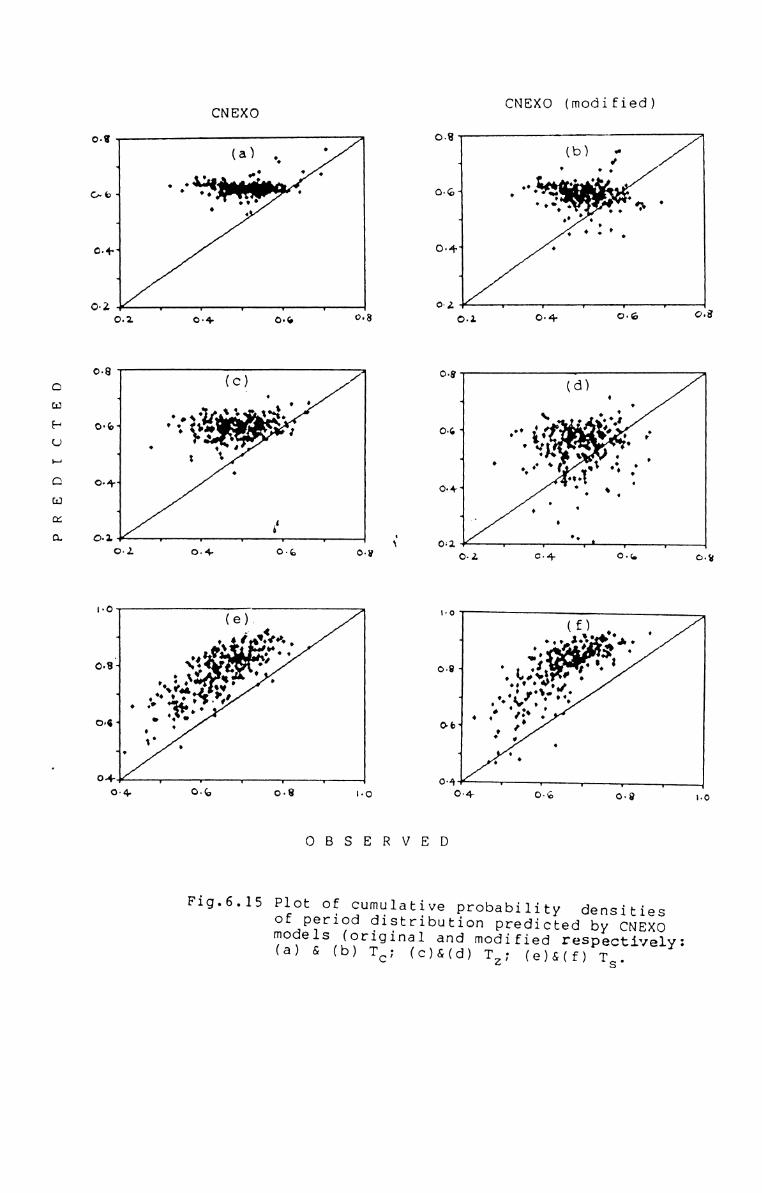
PREDICTED

CNEXO CNEXO (modified)o.3 0-3(a) , ‘ (bi ;1 . ... . . 9 . .9 .Q61 . 0. ,.t 9 0.6-1 . ‘.9 ‘: ‘ .. 090 , ... . . . .5 0. -4 0' . 99 ’ :' .o.q--4 0'4” °4 '1

0'2 v V T Y w ' Y Y Y 8oz 04 as W8 04 04- °@ a0-8 gg _/-4 . ,4 0 .o.‘92r“o $4.. \ . 0.’;Q06‘! 7 0. ’ 0.6+ .00 §.' ‘Q . '.9 O ' V .T 3 ‘o ‘,‘ \ 0.1 O O. 5 ‘ 9 . .9 .9 1. .‘ 9otooufi 0+4 . ~ .0 4-4 O . ‘4‘ J ‘O‘; v V V Y ‘: ' ' ..'#L V Y0.2. 0.4. O Q o.3 O I C 4_ 0.‘. O 8I-O ‘,0‘ 0me? 03,'1 «0°&‘ oe«°-1. ‘ . . .O4. 7 1 I Y 0'4 7 '0¢ 06 08 to 0+ 06 og .0

O B S E R V E D

Fig.6.lS Plot of cumdlative probability densitiesof period distribution predicted by CNBXOm0d€1S (original and modified respectively;(a) & (b) TC; (C)&(d) T2; (e)&(f) TS.

most of the cases. Hence a discussion on the fit based onthis multi-moded distributions is irrelevant and hence notattempted here.

6.3. JOINT DISTRIBUTION OF HEIGHTS AND PERIODS

The joint distribution of zero-crossing heights andperiods are computed for each record, at height intervals of0.2 m and period intervals of l s. Typical examples arepresented in Fig.6.l6. The observed distributions showdifferent shapes depending upon the characteristics of thewaves present in each record. In general, they are deviatedfrom symmetry and are skewed positive. The observeddistributions are compared with the differenttheoretical/empirical models in the following sub-sections.

6.3.1. Comparison of Short-Term Joint Distributionswith Models

In order to examine the fitness of a model with theobserved joint distributions there is no standard test, asseen in the case of wave spectrum. The procedure usuallyadopted is to make visual comparisons of the contours drawnfor the observed and model distributions. Typical examplesof the distributions predicted by time different models ispresented in Fig.6.l7. When there are a large number ofobservations and models, it is difficult to make visual

160

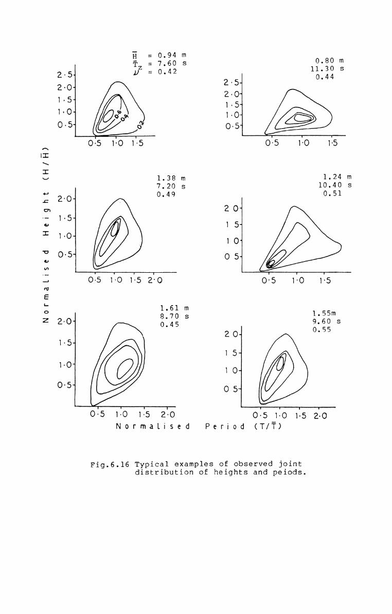
Normalised Height (H/H)

0.94 mis .9-22:2'5‘ : 0'42 0.441.5~ 1.5_‘'040-5‘ 054

0'5 170 15

1,38 m 1.24 m7,20 3 10.40 s2.0‘ 0.49 0.5120*

1-5*1 5*1'0‘ , 10406- 0 5J

ofs 11-0 115 21-0 05 170 :51.61 m

1.55m2~o+ 3:22 5 9.60 s204 0.551.5.

157]'O* 10­O'5" O 5‘0:5 1:0 1:5 21-O 0:5 1:0 1:5 2:0

NormaLised Period (T/T)

Fig.6.l6 Typical examples of observed jointdistribution of heights and peiods.

comparisons. Moreovery eac+| model exhibits characteristicshape of the distribution. A valid statistical test in suchcases is the X? test. In order to use this test, the datahas to be grouped so as to get number of frequencies 1 5 ineach bin (also see Sec.6.3.l). But, such a grouping will

eliminate the tail of the distribution, which are the mostinteresting portion of the height-period distribution forpractical applications. Since run other altrnative if; left,the X? values are computed without grouping the lowfrequencies in the tail (M5 the distribution. Now, thegoodness of fit cannot be made based on the values ofstandard X? distribution with different degrees of freedom.Hence, in order to find the suitability of models adifferent approach is made. For each record a comparisonbetween the values obtained for the different models ismade and the model which give the lowest value of X2 isselected. The model that gives the lowest X2 values inmaximum number of cases is considered as the best among thevarious models. The ‘X? values obtained for different models

is presented in Appendix-B and the results are discussed insub-sections 6.3.1.1 through 6.3.1.5.

6.3.1.1. Rayleigh model

The X? values obtained for Rayleigh (Eq.2.87) rangefrom 26 to 529 with an average around 130 (Appendix-B). This

161

Normalis ed Fieigiit (H/F3)

zoi«5~

«o~

oe­

RAYLEIGH

2-OJ

41-5

1-0 A

0-5

o3 Ho Uszflo

TAYFUN

@06 fio fls do

LONGUET—H|GG|NS(1983)

6% flo flszfio

CNEXO (modified)

0% fio flsNormalised Period (T/T)

GLUHOVSKH2-O1

ms­

i.ooe

ob flo fls

LONGUET-HIGGINSm9fln

2.o1-51

«o~

o.&

ob floihszb

CNEXO2.0-4

1-5

1.0-4

O6~

6% flo H5

Fig.6.17 Typical examples ofjoint distributjonpredicted by diffe­rent models.

nH3del.l1as tzhe Iloweast )(2 vaflluess in <>nl)r 4 causesconstituting about 1% only. When examined according to Hsw,T2 and spectral width ranges, it is found that the very fewcases where the ‘X2 is the least, correspond to lower aswell as higher ranges of H middle ranges of T2 (8-11 s)sw'

and higher ranges of GS. However, since the number of casesof best fit are very few, specific conclusions cannot bedrawn from these observations.

The modes are incorrectly placed tn! this model. Theyare at larger heights and periods when the observed ones arenearer to the origin. But, when the observed modes are atlarger heights and periods, this models place them nearer tothe origin.

The very poor performance of this model may be due tothe positive correlation present between heights andperiods, as against the assumption in developing this model.The observed heights and periods show significantcorrelation in most of the cases, the coefficient rangingfrom -0.06 to +0.77 with an average of 0.41 and a standarddeviation of 0.16.

6.3.1.2 Gluhovskii's model

Gluhovskii's model (Eq.2.89) is also run: found tofollow the observed distribution in most of the cases. The

162

X? values range from 12 to 427 with an average of 128. Thevalues are the lowest in 18 cases which is about 6% of thecases examined. The few cases of best fit obtainedrepresent all the ranges of Hsw, T and spectral widthz

present in the data set. However, the fit is comparativelybetter in the higher ranges of Hsw and lower ranges of T2(Appendix-B). The mode (M5 the predicted distributiondeviate from the observed in many cases, as seen with theRayleigh model. However, the deviations are less in thiscase. On the average, the modes are close to the observedheight values but are shifted slightly to the higherperiods.

6.3.1.3. Tayfun's model

Tayfun's model (Eq.2.98) fit the data in maximum number

of cases (Appendig-B). Generally, the values are lowerwith this model. They range from 15 to 276 with an averageof 73. The X? values obtained with this model are thelowest in 226 cases which is 72% of the data. This model is

found to have representation in all the ranges of’ H butsw'

is not very good in the cases of very low and very high Hswvalues. When the data is grouped in 0.25 m Hsw interval,the X2 values are the lowest in more than 60% for all thegroups in the Hsw range 0.25-1.75 m. Similar fit isobtained in all the T2 and ew ranges present in the data

163

set. When the modes are examined, some deviation isobserved, but are closer to the observed ones.

The better fit obtained in period and jointdistributions with this model indicate the conspicuousdeviation of these distributions from the normal. Since thedistribution of heights are not simulated correctly by thismodel, it may be the period distribution concept of Tayfunthat contribute to the success CM? this model over theothers. Since the present location is a typical example ofshallow water effects due to gently sloping bottom, wherethe transformation processes, especially the bottomfriction, is more pronounced (Kurian, 1987), it isreasonable to conclude that Tayfun's model is suitable forsimulating the joint distribution of shallow water waves.

6.3.1.4. CNEXO models

The original as well as the modified forms of thedistribution suggested by the group of CNEXO (Eq.2.94 andits modification) are found not ix) perform satisfactorily.The X? values range from 12 to 673 in the case of theoriginal form and from 11 to 835 in the case of the modifiedform (Appendix-B). The average'X2 values for these modelsare 148 and 153 respectively. Eventhough the range andaverage are more for the modified form, it has more numberof cases with lowest X? values compared to the original

164

form. when the values are the lowest in 15 cases (5%) forthe original form it is the lowest in 32 cases (10%) for themodified form. Both the forms are found to follow the data

better at the cases of high Hsw values, but deviate in thecases where Tz values are very low or very high.. The modi­fied form has its best fit at the highest HSw°ranges, wherethe Tayfun's model fails. Both the CNEXO models have their

best representation in the T2 ranges between 8 and 12 s. Asregard to spectral width, the original form has its lowest3? values in the range of ew from 0.7 to 0.85 only. Themodified form represents all the ranges present in the dataset, but show better performance in the lowest ranges.

The modes predicted by the first form are found to beshifted considerably to the origin. The modified formpredict the modes at larger heights and periods in the casesfor which the observed modes are nearer to the origin. Onthe other hand, when the observed modes are at largerheights and periods, the predicted modes are found to beshifted towards the origin. In general, both the formspredict the modes shifted to the lower heights and periods,the deviation being large with the original form and lesserwith the modified form. The modes are incorrectly placed bythis model in cases of lower width of spectrum also(Srokosz, 1988). The observation that the modified form fits

165

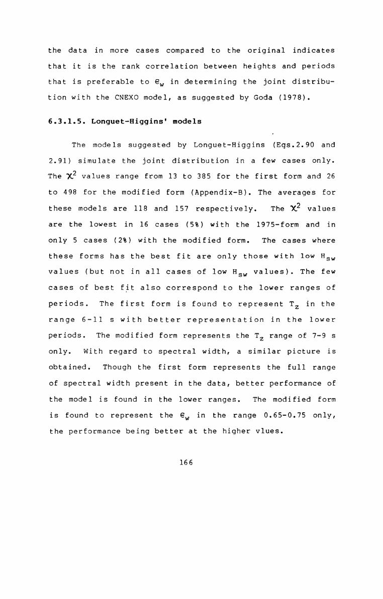
the data in more cases compared to the original indicatesthat it is the rank correlation between heights and periodsthat is preferable to ew in determining the joint distribu­tion with the CNEXO model, as suggested by Goda (1978).

6.3.1.5. Longuet-Higgins‘ models

The models suggested by Lbnguet-Higgins (Eqs.2.90 and2.91) simulate the joint distribution in a few cases only.The X? values range from 13 to 385 for the first form and 26to 498 for the modified form (Appendix-B). The averages forthese models are 118 and 157 respectively. The ‘K2 valuesare the lowest in 16 cases (5%) with the 1975-form and inonly 5 cases (2%) with the modified form. The cases where

these forms has the best fit are only those with low Hswvalues (but not in all cases of low Hsw values). The fewcases of best fit also correspond to the lower ranges ofperiods. The first form is found to represent T2 in therange 6-11 s with better representation in the lowerperiods. The modified form represents the T2 range of 7-9 sonly. With regard to spectral width, a similar picture isobtained. Though the first form represents the full rangeof spectral width present in the data, better performance ofthe model is found in the lower ranges. The modified form

is found to represent the 6%, hi the range 0.65-0.75 only,the performance being better at the higher vlues.

166

The first form predicts the modes at much largerheights and lower periods than the observed. But, when theobserved modes are very close txa the origin, the predictedmodes are at higher periods. The modes predicted by themodified form are at larger heights when the observed arenear the origin and at lower heights when it is an: largerheights. The periods corresponding to the predicted modesare generally lower in most of the cases. However, specificconclusions cannot be drawn in this case also, due to thefewer number of cases available for comparison. Longuet­Higgins distributions are based on narrow band assumptionand are functions of the spectral width parameter. Hence,there is no surprise in the poor fit obtained for thesemodels with the present data having dominant wide bandspectra.

6.4. CONCLUSIONS

Among the different models available for thecomputathmn of short-temn distributhmi of wave heights inshallow waters, the one suggested by Gluhovskii is capableof simulating the observed distribution in shallow waterssatisfactorily. The cumulative probability densities of H,Hsw and Hmax predicted by this model are in agreement withthe data. The modified Longuet-Higgins’ form performs better

than the original and represents the rough sea conditions

167

more accurately. Though the Rayleigh model does not repre­sent the data in as many cases as Gluhovskii's or Longuet­Higgins' modified forms, it fits in a large number of casesand can be considered as 21 good approximation for allconditions, owing txa its simplicity as ea single-parametermodel. Weibull and Goda's models fit in more-cases duringthe rough sea conditions. When P(§) is overestimated by mostof the models, the values of P(H are predicted more ormax)

less closer to the data, except by Ibrageemov's (whichoverestimates the probabilities of all the above statisticalparameters). Very poor fit is obtained with the models ofTayfun, Ibrageemov and CNEXO. The Tayfun's model simulates

the distribution closely with the observed for cases withhigher energy and spectral width and lower T2. The substi­tution of r(H,T) in place of spectral width in the CNEXOmodel is found to improve the performance of the model, butnot to the level required for practical applications. Thebetter fit obtained with the modified form of Longuet­Higgins', though basically Rayleighean, indicates that theeffects of non-linearities add spectral width affect theshallow water wave height distributions. The best fitobtained in the maximum number of cases with the depth­controlled Gluhovskii's function indicates that thedistribution of wave height in the shallow waters are depth­dependant. The effects of non-linearities are accounted by

168

the depth factor in this model. The failure of thefrequency/period dependant Ibrageemov's and Weibulldistributions, compared to the depth controlled models, isindicative of the lesser influence of the wave period in theheight distribution.

Among the various models tried, Tayfun's only cansimulate the distribution of zero-crossing wave periods,that too for the high energy, shorter period monsoonalwaves. The probability densities of Tc, T and Ts predicted2

by this model are closest to the observed. The CNEXO modelsalways overestimate the probability densities. The Rayleig­hean models always underestimate the probability densities

of T2 and lower periods. But, P(TS) values predicted bythese models are closer to the observed with a variationwithin 2%. The substitution of r(H,T) in the CNEXO modelimproves it but not to the level satisfactory for practicalapplications (as seen in the case of height distributions).The inclusion of the effects of non-linearities and spectralwidth in the Longuet-Higgins‘ modified equation make theperiod distribution to deviate more from the observed. Thisindicates that the distribution of period in the shallowwaters are not affected by the non-linearities and width ofthe spectrum as it does in the case of height distribution.

169

The joint distribution of heights and periods arepredicted closest to the observed by the Tayfun's model.Best results are obtained with this model in the heightrange 0.25 < Hsw < 1.75 m. The CNEXO models fail to simu­late the observed joint distribution satisfactorily.However, the parameter r(H,T) in place of spectral widthimproves the model. At high energy cases, where theTayfun's model does not perform satisfactorily, the modifiedCNEXO model finds its application. Better performance ofthis model is acheived at high energy cases with lowerperiods (T in the range 8-12 s). When the modes predicted2

by the Tayfun's model are in agreement with the observedones, those predicted by the CNEXO models are generally atlower heights and periods. The Rayleigh and Longuet­Higgins's models exhibit very poor performance. The modifi­cations made in Longuet-Higgins‘ (1983) equations is notfound to have improved the model to any degree. The X?values obtained with the modified form is in fact larger inmost of the cases.

170

CHAPTER 7

SUMMARY, CONCLUSIONS AND RECOMMENDATIONS

A brief summary along with the conclusions drawn ispresented in this Chapter. On the basis of the observationsmade in the different Chapters recommendations for furtherresearch are given.

7.1. SUMMARY AND CONCLUSIONS

Detailed studies on the spectral and statisticalcharacteristics along the Indian Coasts are limited. As faras the south-west coast is concerned, practically nosystematic study on the wave characteristics are made. Witha view to fill this lacuna, a comprehensive study on thewave climate, spectral. and statistical characteristics ofthe shoaling waves off Alleppey, which is a typical locationalong this coast, is undertaken.

A review of the available literature on the wavespectral and statistical properties reveals that studies onshallow water wave spectrum and the short-term distributionof wave heights are abundant, but that on the distributionof individual wave periods and its joint distribution withheights are sparse. Even for the spectrum and the heightdistribution, a generalised model with universalapplicability is yet to be developed. Different models are

171

suggested for different environmental conditions and theconstants and coefficients vary from model to model. Fieldevaluation/calibration of these models is required toidentify their validity at different locations.

The wave spectral models derived for deep waterconditions generally fail in shallow waters.’ However, theempirical Scott and Scott-Weigel models simulate the shallowwater spectrum in some cases. Most of the shallow watermodels are the modification of one or other of the deepwater models with another transformation model. The finite

depth dispersion relationship formulated tn! Kitaigorodskiiet al. (1975) serves as a foundation for the development ofshallow water spectral models.

Most of the shallow water wave height distributionmodels are modifications of the theoretically sound Rayleighmodel. Owing to the simplicity as a single-parameter model,the Rayleigh form is extensively used even in shallow watersas a first approximation. The depth-controlled forms appearsUs be promising. 'Tme envelope approach also offers scopefor further developments. Models for the prediction ofshort-term distribution of wave periods are very few and theliterature indicates that they are not capable of simulatingthe period distributions satisfactorily. The number ofmodels available for the prediction of the joint

172

distribution of heights and periods are also few. Majorityof them assume total independence of height and perioddistributions. Significant correlation between heights andperiods are reported by many researchers and efforts arebeing made to incorporate the asymmetry of the jointdistribution in the models. This may throw more light intothe characteristics of the joint distribution of heights andperiods in the shallow waters.

The present study is conducted with wave recordscollected systematically from a shallow water location alongthe Alleppey Coast. Waves are recorded at 3 hourly intervalsusing a pressure type recorder. The transducer is installedat 3.5 m below the MWL at a station having a depth of about5.5 m. Data collected during a 4-year period (1980-84) isutilised to determine the wave climate at this location.From the analysis of these records the yearly variation inwave climate is found to be not significant. Hence the datacovering a complete year is selected for the detailed studyof the spectral and statistical characteristics of theshoaling waves. The wave spectra are computed using the FFTalgorithm and the height, period and their jointdistributions are derived using the zero-up-crossing methodof analysis.

173

The wave climate at this location is influenced by thesouth-west monsoonal winds. During May-September the waves

are characterised by larger heights associated withcomparatively shorter periods and narrow spectrum. Low waveswith comparatively larger periods with broad spectrumprevail during October-April. The period May-September andOctober-April may be classified ens ‘rough’ and ‘fair’seasons for this coast. Whereas the Arabian sea is thegenerating area for the waves during the rough season, wavesfrom 2 different and far-away locations - one farther thanthe other - constitute to the wave climate at this coastduring the fair season.

Multi-peakedness observed in almost all the spectra atthis shallow water location is chm; no the co-existence of

wave trains of different characteristics. Hence thesecondary peaks are not at the higher harmonics of the peakfrequency, as observed in some other shallow waterlocations. The spectral peakedness parameter Qp does notshow any characteristic properties with the wave climate,which may be attributed to the prevalence of secondary peaksin the spectra of the shallow water regions. But, thespectral width parameters es, y and fl. do exhibit suchproperties. Hence, these parameters can be used for aqualitative assessment of the swell dominated wave climatein shallow waters. They are depeddent on each other and on

174

the peak periods. The parameters N or Ifl can be used inpractical applications in preference to es, as they arestatistically more stable. The average spectra for differentenergy ranges show dependence of slope of the high frequencyside of the spectrum on energy.

A new spectral model (PMK spectrum) is ‘developed forthe prediction of shallow water waves following the theoriesof Pierson-Moskowitz (1964) and Kitaigorodskii et al.(1975), and is calibrated with the observed spectra. Theobserved spectra are also compared with Kitaigorodskii etal.'s model with Jensen's modification, the TMA model in itsoriginal form and with a few modifications, the Wallopsmodel and the GLERL model (Liu, 1983). The Scott's model and

its modification by Weigel (1980), though originallydeveloped for deep water conditions, are also attempted,considering their reported applicability at some shallowwater locations along the Indian Coasts.

The shallow water dispersion relationship ofKitaigorodskii et al. (1975) is a useful tool to transformthe deep water spectral models to the shallow waters. Themodels derived using this relationship are able to predictthe shallow water spectrum correctly when suitable scaleparameters are used. Those which are functions of the totalenergy are found to be good scale parameters.

175

The models which depend entirely on the peak frequency

simulate the spectrum correctly at high energy cases (HS 32.5 m) only. The TMA model in its original form (with 5 freeparameters) simulate the shallow water spectra in a largenumber of cases. This model is particularly useful for high

energy cases where HS is of the order of 1.4 m and above.The peak energy density is predicted correctly by thismodel, but the total energy is overestimated, especially inthe low energy cases. The average JONSWAP values of thescale and shape parameters are not useful for this location.Average value of the peak enhancement factor 7 for thecases which fit this model is found to be equal to 3.0. The

application of 0q,in place of dJ, make the model topredict the total energy correctly, but the peak energydensity is overestimated. With this modification, the TMAmodel can be used to simulate the shallow water wavespectrum correctly for low energy cases. These are multi­parameter forms and all the required parameters may not bereadily available in all cases. In such cases, the new 2­parameter PMK model can be used for all practicalapplications. The Scott-Weigel model, though basically deepwater one, is capable of simulating shallow water wavespectra, especially in the low energy cases. The totalenergy predicted by this model is comparable to theobserved, but the peak energy density is overestimated,

176

especially at higher energy cases. The coefficients A and Bneed further modification for application of this model forall conditions. The Wallops model finds its application forthe cases with HS > 0.75 and T 3 10 s. In the cases ofP

higher Tp values the total energy is overestimated and thepeak energy density is underestimated by this model. Careshould be taken while applying this model to cases withlarge peak periods.

The short-term distributions of wave heights computedfrom the data are compared with the distribution functionsof Rayleigh, Goda, Weibull, Gluhovskii, Ibrageemov, Tayfun,Longuet-Higgins (1975 and 1983 models) and CNEXO in theoriginal form and with the modification suggested by Vincent(1984). The depth-dependent models simulate the cmserveddistributions better than the others. Gluhovskii's model iscapable of simulating the observed height distributionssatisfactorily at all conditions. Longuet-Higgins‘ 1983 formalso simulates the distribution in a large number of cases,but is more suitable for high energy monsoonal/stormconditions. Weibull and Goda's models are also suitable forthese high energy conditions, but are not as good as theGluhovskii's or Longuet-Higgins‘ models. Tayfun's modelsimulates the distribution correctly in the cases withhigher energy, spectral width and lower periods.Ibrageemov's and CNEXO models fail in most of the cases.

177

The substitution of r(H,T) in place of es in the CNEXO modelimproves its performance, tun: not to an level satisfactoryfor practical applications. The single parameter modelsbased on Rayleigh distribution are good approximations forall wave conditions.

When most of the models overestimate the cumulative

probability density of E, Gluhovskii's function estimatesthe values correctly. It also estimates P(HS) and P(HmaX)values close to the observed. P(H values are predictedmax)

almost correctly by the other models also, exceptIbrageemov's, which overestimates the probabilities of allthe height parameters. This clearly indicates that the dis­tribution of individual wave heights in the shallow watersis depth dependent and is independent of wave periods.

There is no satisfactory model, at present, to predictthe shallow water wave period distributions for allconditions. Among the presently available ones, Tayfun'smodel is the only one capable of simulating it satisfactori­ly in a large number of cases. This model is particularlyuseful for the monsoonal waves with higher energy and lower

periods. It also predicts P(TC), P(Tz) and P(TS) close tothe observed. ‘The Rayleighean models predict P(TS) valueswithin 2%, but always underestimate P(Tz) and other lowerperiod statistics. The CNEXO models overestimate the cumula­

178

tive probabilities of these parameters. The modification ofLonguet—Higgins (1983) to incorporate the effects of non­linearities and spectral band width make the period distri­bution predicted by that model to deviate more from theobserved, indicating that the period distribution in shallowwaters is independent of the non-linearities and width ofthe spectrum.

The joint distribution of zero-crossing wave heightsand periods deviate from symmetry. Though the shape of thedistribution resembles with CNEXO and Longuet-Higgins‘ modi­

fied forms, the modes are incorrectly placed by thesemodels. The Rayleighean models fail to simulate the jointdistribution in most of the cases. Tayfun's model predictsthe modes of the distribution close to the observed. Best

results are obtained with this model in the HS range of0.25-1.75 m. The CNEXO model modified with r%H,T) improves

the model and makes it capable of simulating the jointdistribution correctly for those cases with higher energyand lower periods. For higher energy cases, where theTayfun's model fails, this modified form of CNEXO can be

used, if T2 is in the range 8-12 s, which is the case with-the monsoonal/storm waves. That is, the Tayfun's model canbe used for the low fair weather waves and the modifiedCNEXO model can be used for the high energy monsoonal waves,

to determine the joint distribution.

179

7.2. RECOMMENDATIONS FOR FURTHER RESEARCH

The wave climate at this location during the roughseason is found to be controlled by the monsoonal wavesgenerated in the Arabian Sea. During the fair season wavesfrom 2 distinct and far-away locations contribute to thewave climate here. Similar observations have been made for

some other locations along the west coast of India . Acomprehensive study involving wave generation andpropagation with directional spreading is required toidentify these generating areas. This will enable topredict the wave climate and their characteristics from themeteorological parameters which are now readily available,thanks to the remote sensing satellite.

The function used to compensate thezmtenuation of wavepressure with depth for the computation of the surface waveheight and spectrum is derived from the linear wave theory.Deviations from this theory is identified by manyresearchers and a scale factor (usually called ‘instrumentfactor‘) is recommended. Different values ranging from 1 to1.5 are proposed for this factor. Moreover, some studiesindicate that this factor is not a constant, but is afunction of frequencies. In order to solve this problem andto arrive at a more correct expression to compensate the

180

pressure attenuation with depth further research iswarranted. Also, it has to be examined whether the scalefactor is also a function of wave heights and periods andwill it be sufficient to modify the scale factor toaccurately compute the surface wave heights and spectrum.

The new PMK spectral model proposed in this study could

be tested only for waves with significant height £ 2.5 mwith peak periods in the middle range. Verification of thismodel an: other locations with different environmentalconditions, especially with different bottom slopes andwider range of wave heights, periods and spectral widths hasto be carried out.

Almost all the spectral models assume constant value ofslope for the high frequency side <H5 the spectrum for allenergy conditions. In the analysis cfif the average spectracomputed for different intervals of energies, it is observedthat the slope is proportional to the energy. Furtherstudies are required to understand the intricacies in thespectral slope-energy dependence.

The waves in shallow waters may contain both breakingand broken components. The short-temn distribution of waveheights is influenced by these components. Goda (1970)proposed a ‘breaker index‘ to determine these waves. Thesuggested constants and coefficients appear to vary for

181

different locations. Calibration of this model andmodification, if necessary, have to be carried out fordifferent environmental conditions. This will help todetermine the distribution of heights and their jointdistribution with periods in shallow waters more accurately.

182

REFERENCES

REFERENCES

Aranuvachapun,S. (1987). Parameters of JONSWAP spectralmodel for surface gravity waves-I. Monte Carlosimulation study. Ocean Engng., Vol.14, pp.89-100.

Arhan,M. and Ezraty,R. (1975). Saisie et analyse de Donneesdes courants particulaires au voisinage du fond dans LaHoula litttorale proche du deferlementd La Houilleblanche No.7/8, pp.484-496.

Baba,M. (1983). Wave climate at selected locations along thesouthwest coast of India, Paper presented in the 19thGeneral Assembly of IUGG, Hamburg.

Baba,M. (1985). Long-term wave monitoring along the KeralaCoast - some results. Proc. Nat. Conf. Dock and HarbourEngng., Bombay, pp.E-49-67.

Baba,M., Kurian,N.P., Hameed,T.S.S., Thomas,K.V. andHarish,C.M. (1987). Temporal and spatial variations inwave climate off Kerala, southwest coast of India.Indian J. Mar. Sci., Vol.16, pp.5-8.

Baba,M. and Harish,C.M. (1985). Wave height and perioddistribution off the southwest coast of India, IndianJ. Mar. Sci., Vol.14, pp.l-8.

Baba,M. and Harish,C.M. (1986). Wave energy spectra for thesouthwest coast of India, Indian J. Mar. Sci., Vol.15,pp.144-152.

Baba,M., Harish,C.M. enui Kurian,N.P. (1986). Influence <ofrecord length and sampling interval on ocean wavespectral estimates. Mahasagar - Bull. Nat. Inst.Oceanogr., Vol.19, pp.79-85.

Battjes,J.A. (1974). Surf similarity. Proc. 14th CoastalEngng. Conf., ASCE, Vol.1, pp.466-480.

Battjes,J.A. (1977). Probabilistic aspects of ocean waves,Communications (N1 hydraulics, Department <mf CivilEngineerig, Delft University, Tech. Rep. No.77-2, 52pp.

Battjes,J.A., Zitman,T.J. and Holthuijsen,L.H. (1987). Areanalysis of the spectra observed in JONSWAP. J. Phys.Oceanogr., Vol.17, pp.l288-1295.

183

Bergan,A.O., Torum,A. and TPraetteberg,A. (1968). Wavemeasurements by a pressure type wave gauge. Proc. 11thCoastal Engng. Conf., ASCE, Vol.1, pp.19-29.

Bhat,S.S. (1986). Short-term analysis of wave parameters - Acase study, M.Tech. Thesis, Mangalore University.

Black,K.P. (1978). Wave transformation over shallow reef(Field measurement and data analysis), Tech. Rep.No.78-42, J.K.K. Look Laboratory of CmeanographicEngineering, University of Hawai.

Blackman,R.B. and Tukey,J.W. (1958). The measurement ofpower spectra. Dover Publications, New York.

Boisvert,W.E. (1966). Ocean currents in the Arabian Sea andNorth Indian Ocean. US Naval Oceanographic Office,Washington, D.C.

Bona,J.L., Pritchard,W.G. and Scott,L.R. (1981). Anevaluation of a model equation for water waves, Phil.Trans. Royal Society, A 302, pp.457-510.

Bouws,E., Gunther,H. Rosenthal,W. and Vdncent,C.L. (1985).Similarity of the wind wave spectrum in finite depthwater - I: spectral form, Jounal of GeophysicalResearch, Vol.90 (C1), pp.975-986.

Bretschneider,C.L. (1959). Wave variability and wave spectrafor wind—generated gravity waves, U.S. Army Corps ofEngineers, Beach Erosion Board, Tech. Memo No.ll8,l92pp. '

Bretschneider,C.L. (1963). A one-dimensional gravity wavespectrum, In: Ocean Wave Spectra, Prentice-Hall Inc.,N.J., pp.4l-56.

Bretschneider,C.L. (1977). On the determination of designwave spectrum. Bull. Look Laboratory, Honolulu, Vol.7,ppo

Burling,R.W. (1963). Discussion on ‘The one-dimensional wavespectrum in the Atlantic Ocean and in coastal waters,In: Ocean Wave Spectra, Prentice-Hall Inc., N.J.,pp.3l-32.

Cartwright,D.E. and Longuet-Higgins,M.S. (1956). Thestatistical distribution of the maxima of a randomfunction, Proc. Royal Society, Ser.A-237, pp.2l2-232.

184

Chakraborti,S.K. (1986). Unification of two-parameter energyspectrum models, J. Wat. Port, Coastal and OceanEngng., VOl.112(1)r PP.l73-176.

Chakraborti,S.K. and Coo1ey,R.P. (1977). Statisticaldistributions of periods and heights of ocean waves, J.Geophys. Res., Vol.82 (9), pp.l363-1368.

Chakraborti,S.K. and Snider,R.N. (1974). Wave statistics forMarch 1968 North Atlantic storm. J. Geophys. Res.,Vol.79 (24): PD-3449-3458.

Cizlak,A. and Kawalski,T. (1969).Wave pressure attenuation.Proc. 22nd International navigation Congress, Paris.

Cooley,J.W. and Tukey, J.W. (1965). An algorithm for themachine calculation of complex Fourier series. math.Comput., Vol.19, pp.297-:30!

Darbyshire,J. (1952). The generation of waves by wind. Proc.Royal Society, Ser.A—2l5, pp.299-328.

Darbyshire,J. (1959). IA further investigation «of windgenerated waves. Deut. Hydrogr. Zeit, Vol.l2(1), pp.7­13.

Darbyshire,J. (1963). The one-dimensional wave spectrum inthe Atlantic Ocean and in coastal waters. In: OceanWave Spectra, Prentice Hall Inc. N.J., pp.27-31.

Darlington,C.R. (1954). The distribution wave heights andperiods in ocean waves. Quar. J. Royal Soc.,Vol.80,

Dattatripl. (1973). Waves off Mangalore Harbour—West Coastof India. J.Wat. Harbour Div., ASCE, Vol.99, pp.39-58.

Dattatri,J. (1978). Analysis of regular and irregular wavesand perfomance characteristics cdf submergedbreakwaters, Ph.D thesis, IIT, Madras.

Dattatri,J. (1985). Comparative study <mE zert> up-crossingand zero down-crossing methods of wave record analysis.Proc. 1st Nat. Conf. Dock Harbour Engng., IIT, Bombay,pp.E81-86.

Dattatri,J. (1987). Ocean wave spectra with multiple peaks ­an analysis. Proc. Symposium on short-term variabilityof phys. oceanogr. features in the Indian waters. NPOL,Cochin, pp.l87-189.

185

Dattatri,J., Jothisankar,N., and Raman,H. (1977). Comparisonof Scott spectra with ocean wave spectra. J. Wat. PortCostal and Ocean Engng., ASCE, Vo1.]03, pp.375—378.

Dattatri,J., Jothisankar,N., and Raman,H. (1979). Height andPeriod distributions of waves off Mangalore harbour ­West coast of India. J. Geophys. Res., Vol.84, pp.3767­3772.

Deo,M.C. (1979). Probabilistic analysis ocean waves- astudy. M.Tech thesis, IIT, Madras.

Deo,M.C. and Narsimhan,S. (1979). Probablistic analysis ofocean waves-a study. Report Indian Inst. Tech.,Bombay.

Draper,L. (1967). The analysis and presentation of wave data-.a plea for uniformity. Proc. llnfli Conf. CoastalEl"lgT1g., V0101’

Ezraty,R., Laurent,M., and Arhan,M. (1977). Comparison withobservation at sea of period on height dependent seastate parameters from a theoretical model. OTC 2744,9th offshore Tech. conf., Houston, pp.149-154.

Forrista1l,G.Z. (1978). On the statistical distribution ofwave heights in a storm. J. Geophys. Res., Vol.83,pp.2353-2358.

Forristall,G.Z. (1981). Measurements of a saturated range inocean wave spectra. J. Geophys. Res., Vol.83, pp.8075­8084.

Forristal1,G.Z. '(1984). The distribution of measured andsimulated wave heights as a function of spectral shape.J. Geophys. Res., Vol.89, pp.10547-10552.

Gluhovskii,B.H. (1968). Distribution characteristics of waveparameters and changes in wave action with depth (inRussian). Repu St. Inst. Oceanology, Moscow, Vol.93,pp.98-111.

Goda,Y. (1970). A synthesis of breaker indices. Trans. JapanSoc. Civil Engineers, Vol.2, part 2, pp.227-230.

Goda,Y. (1974). Estimation of wave statstics from spectralinformation. Proc. Int. Symp. Wave Measurement and

Goda,Y. (1975). Irregular wave deformation in the surf zone.Coastal Engng. in Japan, Vol.18, pp.13-26.

186

Goda,Y. (1978). The observed joint distribution of the7_/ periods and heights of sea waves. Proc. 16th Int. Conf.

Costal Engng., Hamburg, Vol.I, pp.227-246.Goda,Y. (1979). A review on statistical interpretation of

wave data. Rep. of the Port and Harbour ResearchInstitute, Vol.l8(l), pp5-32.

/

Goda,Y. (1983). Analysis of wave grouping and spectra oflong-travelled swell. Rep. Port Harbour ResearchInstitute. Vol.22(1), pp.3-ll.

Goodknight,R.C., and Russe1,T.L. (1963). Investigation ofthe statistics of wave heights. J. Wat. Harbour

Gospodnetic,D. and Miles,M.D. (1974). Some aspects of theaverage shape of wave spectra at station ‘India’ (SOON,l9°W). Proc. International Symp. Dynamics MarineVehicles and Structures in Waves (IMECHE '74), Inst.Mech. Engineers, pp.l9-32.

Grace,R.A. (1978). Surface wave heights from pressurerecords. Coastal Engng., Vol.2, pp.55-67.

Harish,C.M., and Baba,M. (1986). On spectral and statisicalcharacteristics of shallow water waves. Ocean Engng.,Vol.l3(3)., pp.239-248.

Harris,D.L. (1972). Characteristics of wave records incoastalzone. In: Waveson beaches and resulting sedimenttransport, Academic press, Inc., pp.1-47.

Harris,D.L. (1974). Finite spectrum analysis of waverecords. Proc. International Conf. Ocean WaveMeasurements and Analysis, ASCE, pp.lO7-124.

Hasse1mann,K, Barnett,T.P., Bouws,E., Carlson,H.,Cartwright,D.C., Enke,K., Ewing,J3 Gienapp,H.,Hasselman,D.E., Richter,K., Sell,W. anui Walden,H.(1973). Measurement of wind-wave grouth and swell decaythe Joint North Sea wave Project (JONSWAP). DeutschesHydrographisches Zeit, Suppl. A, Vol.8(12), 95pp.

Hasselmann,K., Ross,D.B., Mi1ler,P. and Sell,W. (1976). Aparametrical wave prediction model. J. Phys. Oceanogr.,Vol.6: PD.20l—228.

187

Hoffman,D. (1974). Analysis of measured and calculatedspectra. Proc. Int. Symp. Dynamics Mar. VehiclesStructures Waves (IMECHE '74), pp.8-18.

Homma,M., Horikawa,K. and Komari,S. (1966). Response charac­teristics of underwater wave gauge. Proc. 10th Coastal

Houmb,O.G. and Overik,T. (1976). Parameterization of wavespectra and long term joint distribution of wave heightand period. Proc. Behaviour Offshore Structures (BOSS'76), Trondheim, Norway, Vol.1, pp.l44-169.

Huang,N.E., and Long,S.R. (1980). An experimental study ofthe surface deviation probability distribution andstatistics of wind generated waves. J. Fluid Mech.,Vol.lO1, pp.179-200

Huang,N.E., Long,S.R., Tung,C.C., and B1iven,L.F. (1981). Aunified two-parameter wave spectral model for generalsea state. J. Fluid Mech. Vol.l12, pp.203-224.

Huang,N.E., Long,S.R., Tung,C.C., Yuan,Y. and Bliven,L.F.(1983a). A non-gaussian statistical model for surfaceelevation of nonlinear random wave fields. J. Geophys.Res., Vol.88, pp.7597-7606.

Huang,N.E., Long,S.R., Tung,C.C., Yuan,Y; and Bliven,L.F.(1983b). A study on the spectral models for waves infinite water depth. J. Geophys. Res., Vol.88, pp.9579—9587.

Ibrageemov,A.M. (1973). Investigation of the distributionfunctions of wave parameters during theirtransformation. Oceanology, Vol.l3(4), pp.584-589.

Irie,I. (1975). Examinaion of wave deformation with fieldobservation data. Coastal Engng. in Japan, Vol.18,pp.27-34.

Iwata,K. (1980). Wave spectrum changes due to shoaling andbreaking: I, Minus-three-power-law on frequencyspectrum. Osaka Univ., Tech. Rep. Vol.30, pp.269-278.

Jensen,R.E. (1984). Shallow-water spectral wave modelling.Proc. 19th Int. Conf. Coastal Engng., ASCE, Houston,Texas, Vo1.I, pp.547-560.

188

Joseph,P.S., Kawai,S., and Toba,Y. (1981). Ocean waveprediction by a hybrid model - combination of single­parameterized wind waves with spectrally treatedswells. Sci. Rep. Tohoku Univ. Ser.5, Vol.28(l), pp.27­45.

Kahma,K.K. (1981). A study of the growth of the wavespectrum with fetch. J. Phys. Oceanogr., Vol.11,pp.816—827.

Kinsman,B. (1965). Wind waves, Prentice Hall Inc.,N.J.,676pp.

Kitaigorodskii,S.A. (1962). Applications of the theory ofsimilarity to the analysis of wind-generated wavemotion as a stochastic process. Izv. Geophs. Ser. Acad.Sci. U.S.S.R. Vol.1, pp.105-117.

Kitaigorodskii,S.A. (1983). (M1 the theory (ME Equilibriumrange in the spectrum of wind-generated gravity waves.J. Phys. Oceanogr., Vol.13, pp.8l6-827.

Kitaigorodskii,S.A., Krasitskii,V.P., anui Zaslavskii,M.M.(1975). On Phillips theory of equilibrium range in thespectra of wind generated waves. J. Phys. Oceanogr.,Vol.5, pp.410-420.

Kowles,C.E. (1982). On the effects of finite depth in wind­wave spectra: 1. A comparison with deep-waterequilibrium-range, slope and other spectral parameters.J. Phys. Oceanogr., Vol.12, pp.556-568.

Koele,L.A. and [Ma Bruyn, P.A. (1964). Statisticaldistribution of wave heights in correlation with energyspectrum and water depth. Proc. 9th Costal Engng. Cof.,pp.123-139.

Krilov,U.M. (1956). Rep. St. Inst. Oceanology, Moscow,Vol.33, pp.30

Kuo,C.T. and Kuo,S.J. (1975). Effect of wave breaking onstatistical distributions of wave heights. Proc. CivilEngineering in the Oceans-III, Delaware, pp.l2l1-1231.

Kurian,N.P. (1987). Wave height and spectral transformationin the shallow waters of Kerala Coast and theirprediction. Ph.D. Thesis, Cochin Univ. Sci. Tech.

189

Kurian,N.P., Baba,M. and I-lameed,T.S.S. (1985a). Predictionof nearshore wave heights using a refraction programme.Coastal Engng., Vol.9, pp.347-356.

Kurian,N.P., Hameed,T.S.S. and Baba,M. (198flo). A study ofmonsoonal beach processes around Alleppey, Kerala.Proc. Indian Acad. Sci. (Earth Planet. Sci.), Vol.94,pp.323-332.

Lee,T.T. and B1ack,K.P. (1978). Energy spectra of surf waveson a coral reef. Proc. 16th Coastal Engng. Conf. ASCE,Hamburg, Vol.1, pp.588-608.

Liu,P.C. (1983). A representation for the frequency spectrumof wind-generated waves. Ocean Engng. Vol.10, pp.429­441.

Liu,P.C. (1984). On a design wave spectrum. Proc. 19thCoastal Engng. Cof. Vol.1, pp.362-369.

Liu,P.C. (1985). Representing frequency spectra for shalllowwater waves. Ocean Engng. Vo1.12(2), pp.151-160.

Liu,P.C. (1987). Assessing ‘wind ‘wave spectrum representa­tions in shallow lake. Ocean Engng. Vol.14, pp.39-50.

Longuet—Higgins,M.S. (1952). On the statistical distributionof the heights of sea waves. J. Mar. Res., Vo1.l1(3),pp.245-266.

Longuet-Higgins,M.S. (1957). The statistical analysis of arandom moving surface. Phil. Trans. Royal Soc. London,A,

Longuet-Higgins,M.S. (1963). fflna effect <35 non-linearitieson statistical distributions in the theory of seawaves. J. Fluid Mech., Vol.17, pp.459-480.

Longuet-Higgins,M.S. (1975). On the joint distribution ofthe periods and amplitudes of sea waves. J. Geophys.Res., Vo1.80(18): PD.2688—2694.

Longuet-Higgins,M.S. (1980). On the distribution of theheights of sea waves: some effects of nonlinearity andfinite band width. J. Geophys. Res., Vol.85, pp.1519­1523.

Longuet-Higgins,M.S. (1983). On the joint distribution ofwave periods and amplitudes in a random wave field.Proc. Royal Society, Vol.A389, pp.241-258.

190

Manohar,M., Mobarek,I.E, Marcos,A., and Rahul,H. (1974).Wave statistics along the northern coast of Egypt.

Mc Clain,C.R., Chen,D.T., and Hart,W.D (1982). On the use oflaser profilometry for ocean wave studies. J. Geophys.Res., Vol.87, pp.9509-9515.

Mitsuyasu,H. (1969). On the growth of the spectrum of wind­generated waves (II). Rep. Res. Inst. Applied Mech.,Kysusha University, Vol.17, pp.235-248.

Munk,W.H., and Arthur,R.S. (1951). Forecasting ocean waves,Compendium of meteorology, Amer. Met. Soc. pp.l082—1089.

Narasimhan,S. and Deo,M.C. (1979a). Spectral analysis ofocean waves - a study. Proc. Conf. Civil Engng. OceansIV, ASCE, San Fransisco, Vol.2, pp.888-891.

Narasimhan,S. and Deo,M.C. (l979b). Spectral analysis ofocean waves - a study. Proc. Int. Conf. Computerapplications in Civil engineering. Roorkee, pp.V7-V12.

Neumann,G. (1953). On ocean wave spectra and a new method offorecasting wind generated sea. Tech. memo 43, BeachErosion Board, USA.

Ou,S.H. (1977). Pararmetric determination of wave statisticsand wave spectrum of gravity waves. Nat. Cheng KungUniversity, Taiwan, Dissertation No.1-98pp.

Ou,S.H. (1980). The equlibrium range sum the frequencyspectra of the wind generated gravity waves, Proc. 4thConf. on Ocean Engng. in the Rep. of China, Sept.l980.

Ou,S.H. and Tang,F.L.W (1974). Wave characteristics in theTaiwan Straits. Proc. Int. Conf. on Wave Measurementsand Analysis, Vo1.II, pp.l39-158.

Phil1ips,O.M. (1958). The equilibrium range in the spectrumof wind generated gravity waves. J. Fluid Mech., Vol.4,pp.426-434.

Phillips,O.M. (1977). The dynamics of the upper Ocean.Cambridge University Press.

Pierson,W.J. and Marks,W. (1952). The power spectrumanalysis of ocean-wave records. Trans. Amer. Geophys.Union, Vol.33, pp.834-844.

191

Pierson,W.J. and Moskowitz,L. (1964). A proposed spectralform for fully developed wind seas based on thesimilarity theory’ of S.A.Kitaigorodskii. J. Geophys.Res., Vol.69, pp.5181-5190.

Prasad,N.G. (1985). Analysis of waves off Karwar- West Coastof India. M.Tech. Thesis, Mangalore University.

Putz,R.R. (1952). Statistical Distributions of ocean waves.Trans. Amer. Geophys. Union, Vol.33, pp.685-692.

Rachel,C.E. (1987). Analysis of shallow water waves offCalicut: west coast (ME India. Dissertation, MangaloreUniversity, Mangalore.

Rayleigh,J.W.S. (1880). On the resultant of a large numberof vibrations of the same pitch and of arbitrary phase.Philosophical Magazine, Vol.10, pp.73-78, Reprinted inScientific Papers, Dover, 1964.

Rice,S.O. (1944). Mathematical analysis of random noise,Part I-IV, The Bell System Tech. J., Vol.23, pp.282­332.

Rice,S.O. (1945). Mathematical analysis of random noise,Part I-IV, The Bell System Tech. J., Vol.24, pp.46­156.

Rudnick,P. (1951). Correlograms for Pacific Ocean Waves.Proc. Second Berkeley Symposium on MathematicalStatistics and Probability, pp.627-638.

Rye,H. (1976). ‘Discussion on parameterization of wavespectra‘. Proc. Behaviour Offshore Structures (BOSS'76), Trondheim, Norway.

Rye,H. (1979). Wave parameter studies and wave groups. Proc.International Conf. Sea Climatology, Paris, pp.89-112.

Rye,H. (1982). Ocean wave groups. Dept. Mar. Tech.,Norwegian Inst. Tech., Rep. UR-82-18, 2l4pp.

Saji,A. (1987). Analysis of waves off Cochin: west coastof India. M.Tech. dissertation, Mangalore University.

Sawaragi,T. and Iwata,K. (1976). Wave spectrmn of tweakingwave. Proc. 15th Coastal Engng. Conf., ASCE, Vol.1,

192

Scott,J.R. (1965). A sea spectrum for model tests and long­term ship prediction. J. Ship Res., Vol.9(3), pp.145­152.

Scarborough,J.B. (1966). Numerical mathematical analysis.Oxford and IBH Publishing Co., Calcutta.

Seiwe1l,H.R. (1948). Results of research on surface waves ofthe western North Atlantic, Paper Phys. Oceanogr. Met.,Vol.10(4).

Shadrin,I.F. (1982). Deformed wave spectrum in tflma coastalzone. Oceanology, Vol.22, pp.694-696.

Shum,KUT. and Melvi1le,W.K. (1984). Estmates of tflma jointstatistics of amplitudes and periods of ocean wavesusing an integral transform technique. J.Geophys. Res.,Vol.89, pp.6467-6476.

Silvester,R. (1974). Coastal Engineering, Vol.1 - Genera­tion, propagation and influence of waves, ElsevierPublishing Company, 457pp.

Sivadas,T.K. (1981). A tide and wave telemetering system,Pno. lst Indian Conf. Coastal Engng., Madras, Vol.1,

Srokosz,MuA. (1988). A note on the joint distribution ofwave height and period during the growth phase of astorm. Ocean Engng., Vol.15, pp.379-387.

Srokosz,M.A. and.Challenor, P.G. (1987). Joint distributionof wave height and period: a critical comparison. OceanEngng., Vol.14, pp.29S-311.

Sundar,V. (1986). Studies on analysis of ocean wave recordsoff Madras. Proc. 3rd Indian Conf. Ocean Engng. Vol.1,

Tang,F.L.W., Chen,Y.Y. and Lin,S.C (1985). Probabilitydensity function of surface elevation and wave heightof random sea considering nonlinear effect. Proc. Int.Symp. Ocean Space Utilization '85, Tokyo, pp.165-172.

Tayfun,M.A. (1977). Linear random waves on water ofnonuniform depth. Ocean Engng Rep. No.16, Part II,Dept. of Civil Engineering, University of Delaware,Newark, D.E ( Ref. Coastal Engng. Conf. 1978 Proc.)

193

Tayfun,M.A. (1980). Narrow-band nonlinear sea waves.J.Geophys. Res. Vol.85, pp1S48-1552.

Tayfun,M.A. (1981). Distribution of crest-to-trough waveheights. J. Wat. Port Coastal Ocean Div., ASCE,

Tayfun,M.A. (1983a). Nonlinear effects (N1 the distributionof crest—to-trough wave heights. Ocean Engng.Vol.l0(2)r PP.97-106.

Tayfun,M.A. (1983b). Effect of spectrum bandwidth on thedistribution of wave heights and periods. Ocean Engng.,Vol.10(2), pp.107-118.

Thomas,K.V. and Baba,M. (1983). Wave climate off Valiathura,Trivandrum. Mahasagar - Bull. Nat. Inst. Oceanogr.Vol.16, pp.41S-421.

Thompson,E.F. (1974). Results from the CERC wave measurementprogramme. Proc. Int. Symp. On Wave Measurements andAnalysis, ASCE, pp.836-855.

Thompson,E.F. (1980). Energy spectra in shallow US Coastalwaters. US Army, Corps of Engrs., Coastal Engng. Res.Centre, Tech. Paper No.80-2, 149pp.

Thompson,E.F. and Harris,D.L. (1972). A wave climatology forUS Coastal waters. US Army, Corps of Engrs., CoastalEngng. Res. Centre, Reprint 1-72.

Thornton,E.B. (1977). Rederivation of the saturation rangesin the frequency spectrum of wind generated gravitywaves. J. Phys. Oceanogr. Vol.7, pp.l37-140.

Thornton,E.B. (1979). Energetics of breaking waves withinthe surf zone. J. Geophys. Res., Vol.84, pp.493l-4938.

Thornton,E.B. and Schaeffer,G. (1978). Probability densityfunctions of breaking waves. Proc. Int. Conf. CoastalEngng., Vol.1, pp.507-S19.

Thornton,E.B. and Guza, R.T. (1983). Transformation of waveheight distribution. J. Geophys. Res., Vol.88, pp.5925­S938.

Toba,Y. (1973). Local balance zhn the air-sea boundaryprocesses,3, On the Spectrum of wind waves. J.Oceanogr. Soc. Japan, Vol.29, pp209-220.

194

Varkey,M.J. and Gopinathan,C.S. (1984). Programs forspectral and zero-up-crossing analysis of wave records.National Inst. Oceanogr., Goa, Tech. Rep. No.5/84.

Vincent,C.L. (1981). 2; Method for estimating depth-limitedwave energy. CERC,CETA NO.8l-16.

Vincent,C.L. (l982a). Shallow water wave modelling. lst Int.Conf. Meteorol. air-sea interaction coast zone, Am.Meteorol. Soc., Haugiee.

Vincent,C.L. (1982b). Depth limited significant wave height:A spectral approach. CERC, Tech. Rep. No. 82-3.

Vincent,C.L. (1984). Shallow water waves. A spectralapproch. Proc. 19th Int. Conf. Coastal Engng. Housten,Texas, Vol.1, pp.370-382.

Vincent,C.L., Gosskopf,W.G. and Mc Tamany (1982).Transformation of Storm wave spectra in shallow waterobserved during the ARSLOE storm. Proc. OCEANS '82,pp.920-925.

Watters,J.K.A. (1953). Distribution of height in oceanwaves. New Zealand J. Sci. Tech., B, Vol.34, pp.408­422.

Weigel,R.L. (1949). An analysis of data from wave recorderson the Pacific Coast of the United States. Trans. Amer.Geophys. Union, Vol.30, pp.700-704.

Weigel,R.L. (1980). Design wave. Short-tenn course CH1 smallharbour Engng. Vol.1, pp.4.l-4.55.

Wilson,B.W., Chakraborti,S.K. and Snider,R.H. (1974).Spectrum analysis of Ocean Wave Records. Proc. Int.Symp. Wave Measurements and Analysis, Vol.I, pp.87-106.

Yoshida,K., Kajiura,K. and Hidaka,K. (1953). Preliminaryreport of the observation of ocean waves at HachijoIsland. Rec. Oceanogr. Works Japan, Ser l,pp.81-87.

195

APPENDICES

Appendix-A Fitness of the Models for Height and Period-Distributions.c::<—¢¢c1—:-ct¢:——:-n31::--n1::c:::¢::1¢¢z:::—¢cc-—at-cc-——q¢¢——-—-——--acooqo¢—<—:¢-—————:

::—¢:::q1:<::-n—nq-——z:no¢2::::z:::¢—-:::¢::—-—::—-¢c-—on-cg-9:¢—u<c—-¢——-c——.—.a—:<¢q:c——:<1 20129 01-Jan-81 0.73 12 20132 02-Jan-81 0.63 13 20135 03-Jan-81 0.674

5O O O

J:-\.OU‘0t\)o--ua

20138 05-Jan-81 0.5620142 06-Jan-81 0.6020146 07-Jan-81 0.6320149 08-Jan-81 0.9520152 09-Jan-81 0.6920155 12-Jan-81 0.64

13-Jan-81 0.6020162 14-Jan-81 0.5420165 15-Jan-81 0.3620168 16-Jan-81 0.3420171 17-Jan-81 0.32

15 20175 20-Jan-81 0.7916 20179 21-Jan-81 0.6417 20182 22-Jan-81 0.5618 20185 23-Jan-81 0.6319 20188 24-Jan-81 0.6220 20192 27-Jan-81 0.9521 20196 28-Jan-81 0.8722 20199 29-Jan-81 0.5923 20202 30-Jan-81 0.48.24 20204 10-Feb-81 0.6325 20207 11-Feb-81 0.5426 20210 12-Feb-81 0.4227 20213 13-Feb-81 0.6728 20216 16-Feb-81 0.4929 20220 07-Feb-81 0.5130 20223 18-Feb-81 0.4511 20228 19-Feb-81 0.5932 20232 20-Feb-8] 0.4533 20235 21-Feb-81 0.4734 20238 23-Feb-81 0.5135 20243 24-Feb-81 0.7636 20247 25-Feb-81 0.6137 20250 26-Feb-81 0.6138 20253 27-Feb-81 0.7039 20255 28-Feb-81 0.6440 20258 02-Mar-81 0.5741 20262 03-Mar-81 0,5742 20265 04-Mar-81 0.6743 20267 05-Mar-81 0.9844 20270 06-Mar-81 0.7245 20273 07-Mar-81 0.7546 20275 09-Mar-81 0.5247 20279 10-Mar-81 0.5848 20283 11-Mar-81 0.7049 20285 12-Mar-81 0.5550 20287 13-Mar-81 026651 20290 16-Mar-81 0.5852 20294 17-Mar-81 0.5653 20298 18-Mar-81 0.5454 20301 19-Mar-81 0.5555 20304 20-Mar-81 0.57

:1cc:¢::¢:1::-Q:1:1:1:-nqxct-u-czcqocx-oztzx-—-——u-oczuu:——oqu—-o:—n—o¢—-nat-¢1—¢-o.oq—g¢—¢————.o—

I-0 D-4

mu-o\DQ\O\l~JODOCD

00000‘ O 9 H HT H H H H HT IO—Ou—l-doiI—l &LaJNJ-‘©‘~DC'-3\J3\'

IN) :3 0''‘ U1 ND

H H H

0—4U—‘U—“-J 5-JO—‘

4“)©gg©|\_,,.4pQ._a©...au-au_a\.Or—4\.D\O\OC)Qt—of\Jt-4O0—0\O\1)@\D\D\J\OC3©©"‘\O©C\O‘~OCn“$0

. g. o . too 0 O o O 0 ' I 0 0

H H

"i"1"'1 "'i"'i"'1

"'*l"1"1Fi

"'i"i"§

H‘ H H H

F-J5-‘I-iii-l‘—‘.i I III 213$ II

s\)—]ss\—i\\t-iVVO-it-It-it-,‘

~14 Hrfifi *1H H'4

3:

-ia H H "i"5"i"‘1"i "'5*'i'-1"'i"‘1

5-! *-1'-1'-1 '-‘J -1'-1 '-'1'-1-1

I

D—‘ fi‘.'—‘%‘*‘.—‘.-‘O—JF-50-‘ . o g .0 I0 0000 I °° '

:23: I

Has‘ H

'-1"i""1"'i*'] *']"i"i"i

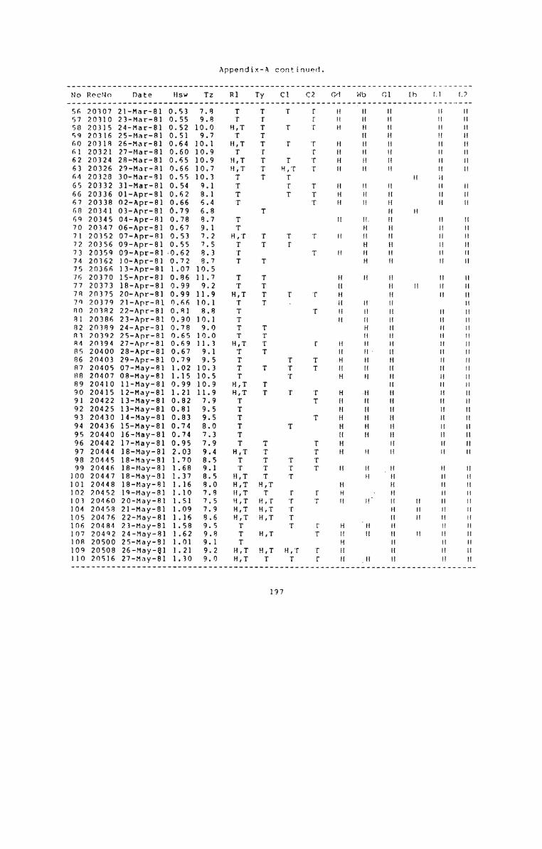
Appendix-A continued.—¢¢———¢——¢:<g—o-:12:-¢c----o-02::-oz:-p-qcunq-p-aco-—cu.-can-cc;-o¢-o—¢--n..¢_.---cccq-n--———_—--—————

No Rocno Date Hsw Tz R1 Ty C1 C2 Cd wb C1 Ih 11 I256 20307 21-Mar-81 0.53 7.8 T T T T H H H H H57 20310 23-Mar-81 0.55 9.8 T T T H H H H H58 20315 24-Mar-81 0.52 10.0 H,T T T r H H H H H69 20316 25-Mar-81 0.51 9.7 T T H H H H60 20318 26-Mar-81 0.64 10.1 H,T T T T H H H H H61 20321 27-Mar-81 0.60 10.9 T T T H H H H H62 20324 28-Mar-81 0.65 10.9 H,T T T T H H H H H63 20326 29-Mar-81 0.66 10.7 H,T T H,T T H H H H H64 20328 30-Mar-81 0.55 10.3 T T T 11 H65 20332 31-Mar-81 0.54 1 T T T H H H H H66 20336 01-Apr-81 0.62 1 T T 1 H H H H H67 20338 02-Apr-81 0.66 .4 T T H H H H H68 20341 03-Apr-81 0.79 8 T H H69 20345 04-Apr-81 0.78 7

_-ae"'1

70 20347 06-Apr-81 0.6771 20352 07-Apr-81 0.5372 20356 09-Apr-81 0.5573 20359 09-Apr-81 0.6274 20362 10-Apr-81 0.7275 20366 13-Apr-81 1.0776 20370 15-Apr-81 0.8677 20373 18-Apr-81 0.9978 20375 20-Apr-81 0.9979 20379 21-Apr-81 0.6680 20382 22-Apr-81 0.8181 20386 23-Apr-81 0.9082 20389 24-Apr-81 0.7801 20392 25-Apr-81 0.6584 20394 27-Apr-81 0.6985 20400 28-Apr-81 0.6786 20403 29-Apr-81 0.7987 20405 07-May-81 1.0288 20407 08-May-81 1.1589 20410 11-May-81 0.9990 20415 12-May-81 1.2191 20422 13-May-81 0.8292 20425 13-May-81 0.8193 20430 14-May-81 0.8394 20436 15-May-81 0.7495 20440 16-May-81 0.7496 20442 17-May-81 0.9597 20444 18-May-81 2.0398 20445 18-May-81 1.7099 20446 18-May-81 1.68

100 20447 18-May-81 1.37101 20448 18-May-81 1.16102 20452 19-May-81 1.10103 20460 20-May-81 1.51104 20458 21-May-81 1.09105 20476 22-May-81 1.16106 20484 23-May-81 1.58107 20492 24-May-81 1.62108 20500 25-May-81 1.01109 20508 26-May-81 1.21110 20516 27-May-81 1.30.—¢¢——¢—a:¢¢-5-ncu-——nu-cc-o-¢—¢¢¢—ca-—--u¢--p-u--———-p—.o-unca-——.._-.--c--———————-——..~—-¢—___—

0-00-J

o-.9»--oooaoxnqxoaaaxmcxho

I

-3-1-1* '-3 '-1-1

-1

H) .

3:23:

H H H H HH H H H HI

-1*-1*-1'-1'-5‘ r-1*-1

*-1

v-1-1’-1'-1 H H" H H)j H H H H Hiii-C T J: H H H H HH H‘ H H II"I

*'<1"'1"1"i

'-1

H H H H IIH H H H III-40-it-40-!

:o:g:.o:o:oa3.\1.~1~.lcoco~oEn~o~1~1cDso~o~1v-OOO:O~D*-'o:O:3O3O

‘ ‘ '-‘I’-1'-3*-3‘

-1

-1'-1'-1

-I

II

-1*-1*-iv-1*-1'-1

>-1'-1 >-1*-i

-1 v-1 '

v-3 -1

II I

. co to 0

Q);-go-—a.p.J1o\\og1gnou'|>—aU1-h\OLa-IOU1U1\O\O\OU'|u)&fi|-‘U900’-‘\3*-'VO‘\)"U1"\UV"'\”"

:z::3:7:. 3:--1--1-1-1*-1»-1

v-1'-1-i -1

-1'-1'-1-1‘—i -41'-1--1

v-1-1-1-1

I

1: :1:

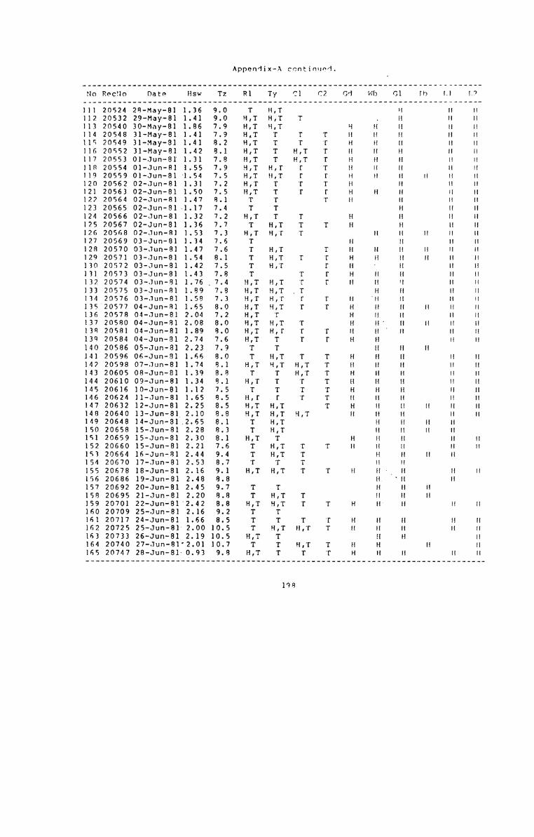
Appendix-A continued.4——¢¢¢¢—¢ct-——¢:-Q----nu-c-cup:--n-o¢--p-nzqcusqq-nu--pg-g-p-o——:¢.o-cu-c-———<c—c-nu-.---c-—.—-——ca...---__—¢—u—

g.-<:—¢¢¢¢c¢-couoccc-o-91-aq--scum‘.-.-q.-up-zczccocn—-o¢¢——q.¢¢¢o-cc.---pa.-—.—-nq-.—-pun..-——--o—«—---——————

1 20524 28-May-81 1.362 20532 29-May-81 1.413 20540 30-May-81 1.864

.2

II: -Iv-I-1

'-<1

.12

20548 31-May-81 1.4120549 31-May-81 1.41

6 20552 31-May-81 1.427 20553 01-Jun-81 1.310 20554 01-Jun-81 1.55

01-Jun-81 1.54120 20562 02-Jun-81 1.31121 20563 02-Jun-81 1.50122 20564 02-Jun-81 1.47123 20565 O2-Jun-81-1.17124 20566 02-Jun-81 1.32125 20567 02-Jun-81 1.36126 20568 02-Jun-81 1.53127 20569 03-Jun-81 1.34128 20570 03-Jun-81 1.47129 20571 03-Jun-81 1.54130 20572 03-Jun-81 1.42131 20573 03-Jun-81 1.43132 20574 03-Jun-81 1.76_133 20575 03-Jun-81 1.89134 20576 03-Jun-81 1.58135 20577 04-Jun-81 1.65136 20578 04-Jun-81 2.04137 20580 04-Jun-81 2.08138 20581 04-Jun-81 1.89139 20584 04-Jun-81 2.74140 20586 05-Jun-81 2.23141 20596 06-Jun-81 1.66142 20598 07-Jun-81 1.74143 20605 08-Jun-81 1.39144 20610 09-Jun-81 1.34145 20616 10-Jun-81 1.12146 20624 11-Jun-81 1.65147 20632 12-Jun-81 2.25148 20640 13-Jun-81_2.10149 20648 14-Jun-81.2.65150 20658 15-Jun-81 2.28151 20659 15-Jun-81 2.30152 20660 15-Jun-81 2.21153 20664 16-Jun-81 2.44154 20670 17-Jun-81 2.53155 20678 18-Jun-81 2.16156 20686 19-Jun-81 2.48157 20692 20-Jun-81 2.45158 20695 21-Jun-81 2.20159 20701 22-Jun-81 2.42160 20709 25-Jun-81 2.16161 20717 24-Jun-81 1.66162 20725 25-Jun-81 2.00163 20733 26-Jun-81 2.19164 20740 27-Jun-81'2.01165 20747 28-Jun-81 0.9331—<c:::¢1:up:a--o::¢-o-o1:-1::-9-1-n—un-ozqztcgup:——un¢:—-zap:-Q-n-n-no-—cn——u.-<31;-on-:¢¢——aq<c¢<—

O l\J O U1 ‘II \D

\l»D\J\J~JsJ\l\D§D\J\l\D\O

sJ|\).b:aU'|I\)U1\OtDt—-h)\O\OOO

I I .'I‘.33I°.IJI32Z12II"_’

,..igp.io-isssss~\1~\s

--i *-i '-<1>-1*-*1-1*-1*-1'-iv-1*-'1--1 xzn 2:: ‘- ~ ~iHvfi~1H‘ ~ H-4—+H

-id —iH

I112

P-iv-'1'-I r-iv-i-1-1­

--lv-'1

v-1 -<l'-1'-1-1'-i-1'-i-1'-1 H ' u u uH u 11 II n n:::: -i»-I-i

H H ' H H Hr-10-1"'1"1""i H H H H H

:I::I::1::.'I::z::::3::x:

._ip—iss\\ss~\v-at-]I—]O-it-‘V

'-i*"1"i"i"1"')*'i"‘1 v-J-n-1 '-i--iv-ir-iv-1 ’-1’-i '-:'-i I: I :3: :3:

x -I gS Q

--~) 1

LII: I

g_ap_;\us5-is o—!\

"‘1°"1'-i '-1'

"1"1*-1'-1"'3"i*‘1TTT H H H HT H H H HTT

T

9. . 00- '

m-qu1mxnn:mcn~;m-~:Acn-wr-u>munu1~<D-O~D°‘O<DNJOL4°°5‘”U‘“‘“°‘W

2

0-1'-1*-1‘

0-1

I::

v-1'-3--1--1

I

H H H'1‘ H H IIT .I-00-00-!

\.OC)©Q®\O®®\OsD\D®\O\l®®®tI)ODsD\l~.DG)~D®\J\l\D®\l®\l~J\J\J\J®\l\.l\J\J~J. .. .... . . . . . . . . . . 0 0 0 o to 0 0

I I '-I ‘-1

I II

*-1'-1'-i‘>-1"i“'-1

>-1 v-1'-1

2'.

Appendix-A cowtinund.¢¢.—¢——q-¢-o—n--—n¢—ca-o-.¢::¢-n--—1:-n¢—¢¢¢--—¢¢cqpaocuu————o-n——-o¢c—:—n--—<-o——..4-o.———.~¢ . - .——_.

No Rncnn hate Hqw Tz R1 Tv C1 07 Cd wh ml Th 11 17166 20757 29-Jun-81 0.65 8.3 H,I I I I H H H H H167 20764 30-Jun-81 0.48 8.9 I I I H H H168 20768 01-Jul-81 0.60 10.0 I I I H H H169 20776 02-Jul-81 0.67 10.0 H,T ' T H H H H H170 20784 03-Jul-81 0.78 10.0 H,T T H H H H H171 20792 04-Jul-81 0.85 9.4 H,T T T T H H H H H H172 20800 05-Jul-81 1.00 7.8 H,T T H H H H173 20808 06-Jul-81 1.34 7.2 H,T T T T H H H H H174 20816 07-Jul-81 1.60 8.3 H,T T I I H H H H H178 20824 08-Jul-81 1.46 7.9 H,I I I H H H H H176 20832 09-Jul-81 1.36 8.5 H,I I I I H "H H H H177 20840 10-Jul-81 1.20 8.3 H,T T T T H H H H178 20848 11-Jul-81 1.60 8.5 H,T T H,T T H H H H H179 20855 12-Jul-81'1.48 8.3 H,T I H H H H H180 20863 13-Jul-81 1.22 9.2 T T H H H181 20871 14-Jul-81°1.03 8.6 H,T T H,T T H 'H H H H182 20879 15-Jul-81 0.96 9.0 H,I I I I H “H H H H183 20887 16-Jul-81 0.67 7.6 H,I I I H H H H H184 20894 17-Jul-81 0.71 8.2 T T H H H H H185 20902 18-Jul-81 0.58 9.2 H,T T T T H H H H H186 20909 19-Jul-81 0.38 8.6 T H H H H187 20916 20-Jul-81 0.44 7.2 H,T T T H H H H H188 20924 21-Jul-81 0.47 8.3 T T H H H H H189 20931 22-Jul-81 0.80 ‘9.0 T T T H H H H190 20939 23-Jul-81 1.09 8.6 H,T T ‘T T H H H H191 20947 24-Jul-81 1.48 8.1 H,I I I I H H H H H192 20955 25-Jul-81 1.75 9.4 I I H H H H H193 20963 26-Jul-81 2.17 10.3 H,T T T H H’ H H H H194 2097] 27-Jul-81 1.25 9.1 H,T T T T H H H H195 20975 29-Jul-81 1.50 11.3 H,T H,T T T H H H H196 20983 30-Jul-81 1.17 9.0 H,I I H,I I H H H H197 20991 31-Jul-81 1.68 9.5 H,I I I H H198 20995 01-Ann-8] 1.33 9.5 H,T H,T T H H H H199 21000 03-Aug-81 1.46 9.6 H,I H,I H H H200 21008 04-Aug-81 1.77 10.6 I H,I I I H H H H H201 21011 05-Aug-81 0.90 9.8 H,T T H T H H H H H202 21019 06-Auo-81 0.71 8.6 T T H H H H H203 21027 07-Aug-81 0.82 9.9 H,T I I T H H H H H204 21035 08-Aug-81 0.88 9.4 I I I H H H H H205 21043 09-Aug-81 1.00 7.9 H,T I I H H H H206 21051 10-Aug-81 2.32 9.8 H,I H,T H,I I H H H H H207 21056 31-Aug-81 0.28 8.6 T T H H H H208 21060 01-Sep-81 0.64 11.5 H,T T T T H H ‘H H209 21067 02-Sep-81 0.53 9.6 T T T T H H H H H210 21074 03-Sep-81 0.24 8.3 H,T T T H H H H H211 21081 04-Sep-81 0.16 8.2212 21095 06-Sep-81 0.19 10.6 H,T T T H H. H H H213 21101 07-Sep-81 0.61 7.9 I I T H H H H H214 21107 08-Sep-81 1.90 9.6 T H,T T T H H H H H215 21115 09-Sep-81 1.24 8.7 I I I H H H H H216 21123 10-Sep-81 1.09 7.7 T T T H H H H H217 21131 11-Sep-81 1.24 9.4 I H,I H,I I H H H H H218 21136 12-Sop-81'0.78 7.0 I T I H H H H H219 21144 13-sop-81 1.28 8.2 H,I ",T I H H H H H220 21152 14-Sep-81 0.79 8.1 I I H H H H H———¢—¢:——¢¢¢:—¢¢c¢-o-ounqo--occ-caac-:1:-¢¢¢:———-¢—o¢¢cc.-—-.-.—-pq¢¢.-————q--ca-q--—¢-—-¢————

Appenflix-A :ontinun1.—-o-......------........—..-_¢_-.-..———--o—-.—--——-¢_-.._‘.._._..----4..—...—-..~.J’..-..-.-.---_-. oaa . -c--—No ROCNO Date Hsw T2 81 Ty C1 C2 C4 Hh G1 1h L1 L2

<4:———¢x¢c¢:—--o-.—o¢g-n-n<¢¢¢-¢¢¢:-nu--uncxc-1:19upqpqnqp¢-nqqu-—¢¢-..—-.13.-¢—u—.¢--n-p-oa¢—4———c¢«_g<:

H H 11 11 I1.._ .’ H H H H224 21181 18-Sep-81 0.36225 21184 19-Sep-81 1.36226 21192 20-Sep-81 1.45227 21200 21-Sep-81 1.42228 21207 22-Sep-81 0.93229 21215 23-Sep-81 0.84230 21224 24-Sep-81 0.83231 21231 25-Sep-81 0.52232 21238 26-Sep-81 1.42233 21246 27-Sep-81 1.19234 21248 28-Sep-81 0.75235 21256 29-Sep-81 0.44236 21262 30-Sep-81 0.47737 21270 01-Oct-81 0.36238 21276 02-Oct-81 0.29239 21284 03-Oct-81 0.36240 21290 04-Oct-81 0.21241 21297 05-Oct-81 0.28242 21305 06-Oct-81 0.17243 21320 08-Oct-81 0.20244 21326 09-Oct-81 0.30245 21334 10-Oct-81 0.40246 21338 12-Oct-81 0.32247 21350 14-Oct-81 0.43248 21358 15-Oct-81 0.38249 21366 16-Oct-81 0.24250 21373 17-Oct-81 0.34251 21381 18-Oct-81 0.29252 21389 19-Oct-81 0.28253 21397 20-Oct-81 0.51254 21405 21-Oct-81 0.65255 21413 22-Oct-81 0.69256 21421 23-Oct-81 0.68257 21429 24-Oct-8] 0.59258 21437 25-Oct-8] 0.42259 21444 26-Oct-81 0.47260 21451 27-Oct-81 0.54261 21456 28-Oct-81 0.58262 21457 31-Oct-81 0.84263 21459 02-Nov-81 0.56264 21466 03-Nov-81 0-43265 21473 04-Nov-81 0.41266 21476 05-Nov-81 0.32267 21484 06-Nov-81 0.34268 21492 07-Nov-81 0.26269 21500 08-Nov-81 0.27270 21507 09-Nov-81 0.36271 21514 10-Nov-81 0.22272 21522 11-Nov-81 0.17273 21530 12-Nov-81 0.14274 21537 13-Nov-81 0.18275 21545 14-Nov-81 0.21276 21548 16-Nov-81 0.32 1

IISLII

H H H H12 -1

»v-— po­ —— -an H H HH H HI-lL—J

uawt».1~<3n:o~q-wnuna-oc>O\o~J<<hO‘<<D0><<D-1* ..., g o o.ooooo so 0

"1""1"‘|'-1‘

_.T.‘-1

I-if-'il'i!

4

"1 "'1 I I

--v­ -5‘

-n

.4­ ——u-­ -v­ _a­

­ .-o —— un­

|i5—‘O-H0-‘I-3

2133'. I

I-‘o—i|-’\§b—‘\.h-‘H

14w H "'1 "1' ""1I L

s -1p—j

"1 1 "'i"1"-1"'1"i

0. 0 0 O

qk3c)©‘)‘p._ogg\JQ.l.nuasJJ'x0--.ts&\£)1\)*-‘VOUTIDF-00-'\I)\AlC)~O

T: I I 3'.H H H H H3:333.‘ .

us ._i\‘sp-‘Q

"1"1*‘i .23: 8 H u n nu n u u nu u H H Ha—0§_ob—Ip_oh-HI-40-4

TF,T H H ‘H H H HI

TF

|—ap_a 5-00-15-40-10-—li—0|—0D-I

.,.,..,:"‘3‘..,_,;‘i‘_,.“:‘;“.‘;"‘.,:"f“‘“‘

1-1-1 1-1>-1 '-5*-1*-5*-1'-1 -1°-1-41-1 °-1-1'-1

*-1-i-1'-1'-1*-1'-i -i '-1*-<1 --1

d H ~iH'iH~w H H v-3 '-1-1*-1'-5 --:*1 3: 22 II: : ".2 .''.‘...‘'Z‘.. 1‘.

H H H H H#1 r T H H u_ H H n

0-0

‘~13~l\J\O\JO\©\D®\.D\D\.D®~.D©0-‘\O\D‘‘‘1'\)’'''‘‘''‘’'‘'\J’''‘

. 0 0.0. 0 I 0 0 0 O 0 0

wo-omuwwsix:-I>u1m.:>~ou1«J'sa\Au1aJa\m--»DU1~D~J~!J

>-1-1 -<1’-1*-1*-<1 -1 *-1

o-—-.—a-a-—-ococnc-u——u-app.-— uno-.._:-coa-——-cu-c-up-——¢¢-——o—-p——.——¢———-——--c-——9--—-.———.———.._--.-..-_.--.—--—-—­

_ .. _-0 o.-- .—-...—.———-o.--o-oac.qaaco¢¢¢--o-o¢——-o-Q-o-o¢¢-c-u¢¢-n-—.—c—-—ac-p—¢-—.¢—c ca—¢..o—¢--ac cue-.. —- —

¢¢¢c¢¢c¢¢4—oq—¢¢¢-o:¢9:¢:¢:—¢co:c-otzQ-o-occccc-u--:-oz:—q<cu¢—-—-onco-1-o-o-q<-¢--¢——¢—¢——-———*2184821536218632157121577215812158921597216082161321621216232162721632216392164621648216512165721663216702167221680216882169621704217122172021728217352174321751217592176721774217822178921796218022180421810

16-Nov-8117-Nov-8118-Nov-8119-Nov-81'20-Nov-8121-Nov-8122-Nov-8123-Nov-8124-Nov-8125-Nov-8126-Nov-8127-Nov-8128-Nov-8129-Nov-8130-Nov-81.01-Dec-8102-Dec-8103-Dec-8104-Dec-8105-Dec-8106-Dec-8107-Dec-8108-Dec-8109-Dec-8110-Dec-8111-Dec-8112-Dec-8113-Dec-8114-Dec-811S-Dec-8116-Dec-8117-Dec-8118-Dec-8124-Dec-8129-Dec-8126-Dec-8127-Dec-8128-Dec-8129-Dec-8130-Dec-8131-Dec-81

5-! I-1

19..-uoa\.x>cn~o--N’-‘xDOO"‘

O O

I—JI—l

._....4;_; L-dh—l

\J\,a3mc)a;m\o»o\oo)o-c)u—o\4JuO\OLDC)--<1)~O\O~.uOO

.. 0 0 O 9

. 0 9 00 00q’xgd\n\ga\\o\osaO\uJ©~.n©VO\JJb\J0-‘U-Jl’\)U'\@-B‘nO'\~J$J1d‘$‘7‘1-A‘\4nx

onsowhmw

Appenflix-X continued.

-'1

.44 _,a.4 a.4.aa -aw are-sa-+~aa-4

"i'-1'-1

"1"! '1

'-i "i'-1'-1"!

H n H HH H ' H uu H u u nH H H HH H H H

H H H HH H H HH H H I1H H 11 H

H H H HH H 11 HH H H H H

H

I1

H

11

I1

H

H

H

H

H

H

H

H

II

H

H

H

H

H

H

II

———:c@:¢:1¢¢¢¢::¢—g¢¢:¢—:—o-33::11:.-3:--o¢:—.——¢—p¢-o-¢cc:-q-p—-on.-o-ca--—-c-4-pa-——¢——_.n—¢g -_RecNo: Record identification number.Models - R1: Rayleigh: Ty: Tayfun's; C1,C2:Cd: Goda's; wb: weibull: G1: 61uhovskii'3:Ll,L2: Lonquet-Higgins‘ (1975 and 1983).

C‘1E‘..‘(0Ib:

(oriqinal and mm-11fi¢"1):‘H7n3neem0v'3:

201

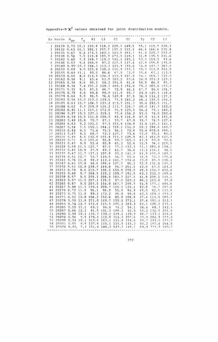
Appendix-n X?‘ values obtained for joint distribution models..--_q<—-4-.--.-e¢¢—o-.--o—_.-o-un--—o—-.-—-a¢—-.-—¢-.-a—-----.-_o—-—can----.-~—

No R0000 Hsw T2 R1 L1 C1 C1 Ty F2 121 20129 0.73 10.3 150.8 118 3 229.5 149.5 55.1 115 9 220.32 20132 0.63 10.1 305.1 257.7 137.2 332.4 66.4 166.4 232.93 20135 0.67 8.2 173.5 142.1 343.5 163.7 61.4 220.7 152.04 20138 0.56 7.5 113.9 180.0 473.9 110.3 51.9 135.5 231.66 20142 0.60 7.9 168.9 110.2 541.1 190.2 52.0 159.9 93.66 20146 0.63 9.4 160.0 97.2 217.3 147.4 42.9 158.9 135.07 20149 0.95'10.3 244.3 112.3 115.9 192.6 74.8 187.7 267.58 20152 0.69 9.0 225.9 149.4 156.9 193.5 59.2 212.0 243.09 20155 0.64 11.1 90.5 86.6 67.0 72.0 35.6 61.1 113.5

10 20159 0.60 8.6 214.9 124.9 119.9 227.9 54.1 168.3 122.011 20162 0.54 -9.1 63.4 61.8 165.2 63.6 34.9 203.8 129.312 20165 0.36 8.6 90.5 59.2 394.6 91.6 58.8 66.0 85.313 20168 0.34 7.4 201.1 118.5 460.3 184.9 70.3 205.6 153.914 20171 0.32 8.5 47.5 46.7 72.0 46.4 67.7 94.6 104.715 20175 0.79 9.0 99.8 90.0 111.0 95.7 29.9 120.5 118.616 20179 0.64 9.0 96.5 76.6 140.9 97.9 36.9 134.2 127.517 20182 0.56 10.0 212.4 129.5 75.9 243.2 46.4 125.0 104.218 20185 0.63 10.7 104.0 133 2 213.7 101.3 38.4 292.5 151.719 20188 0.62 9.9 219.9 126 2 115.7 226.7 49.0 141.9 142.020 20192 0.95 11.1 117.1 172 0 95.9 120.5 54.2 79.1 160.221 20196 0.87 10.5 127.1 218 5 73.6 154.2 53.5 74.0 202.622 20199 0.59 10.0 111.0 109 0 89.9 116.8 47.9 93.9 155.923 20202 0.48 10.9 70.7 87 1 50.7 67.9 39.7 74.5 127.424 20204 0.63 9.2 123.1 97 5 355.6 130.9 33.6 120.3 143.125 20207 0.54 7.5 155.1 184.2 159.1 154.9 59.3 296.6 140.726 20210 0.42 9.2 73.4 75.5 86.1 72.8 55.6 605.6 190.127 20213 0.67 9.5 68.7 72.3 127.7 73.6 53.0 93.1 84.328 20216 0.49 8.5 132.0 103.4 215.3 129.9 42.3 161.0 143.929 20220 0.51 8.3 105.6 86.8 99.3 165.5 43.9 93.8 02.630 20223 0.45 9.0 53.4 80.9 65 2 52.6 52.9 76.3 215.331 20228 0.59 11.5 120.7 97.5 77 3 132.3 51.3 289.9 139.132 20232 0.45 10.9 37.9 49.3 61 7 36.6 33.2 134.1 94.533 20235 0.47 11.7 127.1 107 8 93 2 141.8 64.9 105.9 149.534 20238 0.51 12.7 59.7 140 6 54 7 60.6 32.5 73.3 175.435 20243 0.76 11.9 99.2 112 4 141.7 104.6 32.0 85.9 106.436 20247 0.61 10.9 94.6 109 4 127.7 96.2 52.9 131.9 145.237 20250 0.61 10.9 238.8 149 8 96.7 251.5 42.0 67.6 149 238 20253 0.70 9.4 215.7 106 2 150.0 208.0 49.9 154.7 402.439 20255 0.64 9.7 164.5 135.3 109.7 191.5 62.3 232.2 165.610 20258 0.57 9.5 209.3 208 8 189 7 227.9 44.9 208.2 14 .141 20262 0.57 11.5 207.1 126 5 97 6 240.2 86.3 163.8 97.042 20265 0.67 9.0 207.5 154 0 167 7 208.0 54.9 177.1 404.643 20267 0.98 11.5 130.4 208 7 125 5 124.1 92.8 76.7 197.644 20270 0.72 11.9 86.1 86 0 55.9 94.9 49.0 82.5 133.815 20273 0.75 11.9 89.3 172 2 96.9 90.8 42.5 109 4 199.246 20275 0.52 10.9 104.2 152 6 80.8 108 8 37.4 113 9 180.747 20279 0.58 11.9 271.0 149 7 155.5 272.1 37.4 301 4 212.348 20283 0.70 12.7 173.6 115 5 105 3 189.2 63.1 128.2 239.410 20285 0.55 11.1 69.1 94 4 74.2 56.1 34.4 68.3 142.350 20287 0.66 12.2 91.0 101 3 109.2 92.0 52.2 132.5 204.051 20290 0.58 10.1 136.7 130 1 118.1 139.8 46.7 133.1 204.652 20294 0.56 9.5 179.3 112 8 314.3 207.6 39.9 204.9 177.253 20298 0.54 10.1 310.6 163 1 111.9 334.6 50.7 193.0 157.954 20301 0.55 9.9 137.9 115 1 115.5 145.2 4 .2 107.4 164.555 20304 0.57. 7.3 151.4 146 3 627.7 146.1 69.0 237.9 920.5

C-cc-1--ncc—-oc-o¢-ac;--¢-our--nu-q-o-—-—-p-.¢:—-o¢-.-p———¢———-—--—¢-oo oo--n_—-—

Appendix-B continued.——»—.-—-o¢—-aco-o-o-noQQ-.¢<¢<¢¢—n—¢¢-p¢-1-—¢—n¢-n¢—o-o—o—.-o-o—nc—a¢—¢¢¢-4-o--n-n~o—

No Rheum Hsw T7 R1 Ll C1 C1 Ty C? 1?56 20307 0.53 7.8 88.9 85.7 102.5 93.3 42.4 174.9 .72.157 20310 0.55 9.8 74.7 59.5 11.7 73.7 34.1 154 7 189 158 20315 0.52 10.0 122.9 105.4 122.7 132.0 37.1 211 9 146.850 20316 0.51 '9.7 125 8 86.8 78.1 130.7 32.2 195.1 195 460 20318 0.64 10.1 93.8 94.7 73.7 91.8 27 4 76.4 97.961 20321 0.60 10.9 118.7 90.3 95.6 124.1 27.4 215.4 131.562 20324 0.65 10.9 112 6 124.5 163.9 120.5 5019 141.0 160.061 20326 0.66 10.7 125.8 152.7 64.8 144.6 31.9 171.4 155.561 20328 0.55 10.3 59.9 78.3 95.6 55.9 30.7 111.5 147.965 20332 0.54 9.1 165.6 108.6 297.4 219 5 40.0 120.6 117.966 20336 0.62 8.1 206 5 179.6 129.6 220.3 80.7 147.3 140.967 20338 0.66 6.4 117.5 94.9 472.0 127.1 60.3 271.2 85.168 20341 0.79 6.8 79.5 89.6 111.6 75.2 40.9 94.8 71.869 20345 0.78 8.7 274 5 149.9 330.9 249.9 50.5 190 0 241 670 20347 0.67 9.1 89 1 88.1 175.9 91 1 11.9 346.5 175.571 20352 0.53 7.2 73 1 72.0 249.6 74 4 39.6 115 9-147.572 20356 0.55 7.5 102 1 98.8 400.3 107.9 41.7 175.7 194.573 20359 0.62 8.3 61 6 75.6 81.7 61.4 42 9 93.1 90.474 20362 0.72 .8.7 157 3 135.9 120.3 182.7 .4 4 180.2 181.375 20366 1.07 10.5 206 7 129.7 175.8 259 7 68 8 144.0 221.976 20370 0.86 11.7 221.1 144.4 149.0 197.2 68.9 124.5 189.577 20373 0.99. 9.2 118.3 106.3 232.1 112.4 37.0 50.4 190 779 20375 0.99 11.9 87.5 89.0 91.0 79.8 56.0 107.4 155.179 20379 0.66 10.1 211.0 157.5 212.6 220 2 45.9 105 4 130 180 20382 0.81 8.8 268 6 161.4 672.7 263.6 52.6 108.6 234.581 20386 0.90 10.1 131 6 166.7 156.5 131.9 71.1 158 1 208.192 20309 0.78 9.0 179 4 153.3 227.0 199.6 69.1 227.6 172.583 20392 0.65 10.0 145.2 120.1 302.4 164.9 44.9 143.9 199.784 20394 0.69 11.3 59.5 104.1 69.8 61.2 41 0 147 0 231.485 20400 0.67.'9.1 217.7 150.7 229.0 210.4 79.8 250.6 168.086 20403 0.79 9.5 270 6 198.2 200.8 274.8 86.8 315.0 199.087 20405 1.02'10.3 116 3 384.5 105.7 113.8 55.2 316.4 181.198 20407 1.15 10.5 342.0 290.4 221.6 366.1 154.9 312.1 246.689 20410 0.99 10.9 187 1 126.7 114.1 186 2 79.6 181.7 171.100 20415 1.21 11.9 154.5 104.0 100.6 165 7 79.7 180.8 154.891 20422 0.82 7.9 229 3 159.1 358.9 219.9 73 1 145.5 170 292 20425 0.81 -9.5 329 8 193.2 157.8 311.5 100.1 154.2 311.293 20430 0.83 9.5 279 8 260.7 152.8 250.2 95.2 179 8 216.094 20436 0.74 8.0 171.9 130.4 230.1 167.3 47.7 126.9 145.295 20440 0.74 7.3 249 6 194.1 188.9 246.6 56.3 210.4 131.996 20442 0.95 7.9 138 8 134.2 130.6 145.9 75 2 179.4 136.997 20444 2.03‘ 9.4 171 6 255.0 189.6 147.9 172 1 190.7 118.298 20445 1.70 8.5 178.9 220.4 151.7 215.1 184 2 156.1 296.099 20446 1.68 9.1 203 4 203.1 111.5 267 4 107 4 156.6 194.1100 20447 1.37 9.5 139.4 149.8 102.9 157.0 116 1 139.5 151.9

101 20448 1.16 ;8.0 114.8 103.0 144.3 110.2 97.3 246.1 164.9102 20452 1.10 7.8 76.5 94.8 91.9 56.9 49.4 110.0 141.3103 20460 1.51 7.5 112.0 106.9 131.2 114.8 96.9 129.5 167.4104 20458 1.09 7.9 71 2 65.3 71.9 63.3 45.8 172.7 117.7105 20476 1.16 8.6 82 2 96.7 119.2 77.6 79.4 95.5 104.3106 20484 1.58 9.5 123 9 168.9 93.1 133.2 147 6 93.1 135.5107 20492 1.62 9.8 175 3 189.3 186.4 159.6 135 8 225.3 272.0108 20500 1.01 9.1 154.5 154.8 186.4 189.3 71 7 154.4 120.0109 20508 1.21 9.2 97 7 81 8 84.5 101 8 55.1 120.6 120.4110 20516 1.30 9.0 135 6 108 9 82.2 153.3 68.4 113.0 131.8——xaq-oqczc-.¢..—n:¢qo¢-nu--up-o-o¢-q-:-as--n-c-¢-oz-qguo-o---.o..—o—cq-ac-—-—-o-go--—¢¢

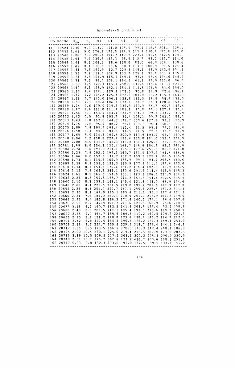
Appendix-8 Ccntinuod—....--__-.-¢——nup-o—¢-¢o¢-on--.¢q——oo-n-pcc-o4o¢—n——-pug--.—-————. -—_q-————.———

—:q-——-—¢-ac:-co¢¢-.1-p-o¢¢¢—n—.—¢-o-n-nq-—-——-¢¢—qp-p-¢¢¢——-o--w-—--.--n-o.-o­

I—Jo——b—I

-.p:)Q)©.n\oa)m\O®~O-Isl)\JJ)msD®®®\lCD~DCDCDxisJCDLD\J~.D\l~JxJ~J\J-D\l\J\)~J. . 0.0 0 0-0 0 0000 0 0'

~J~J\fi\J\J\J\J\JsD«fi\J\l‘~D\O

000

. . Q . g 9. 0.00 0 0 O0 0 0 C\\D©|\)\3Lunn-ts.n\_nn.aJ'\O\UJ\J|\).b'dU'|f\JU1\O®""f\)~D\D\3O

ol 0 0000 0 0 0

a)~Ju1U'|U1l\)G)Q)s.l\.D>-o\J.£-G\t--ulr-\DU1U1U1*-‘~b*-‘-3&0

CO to

. . . . . . .. . .. . .. .. . . . . . q . g . Q . O . 00 Q0 0 0 .0 0N)\j(_.;p—oy_o\]g'|o-4\j\J'\u-o-hu.)\LJ\Jka-It-—o.£LL,.;&d’\uJ.&l'\)tD‘Jo-\lq)~A)t—oLdJ4-O-‘U-F-‘Ul\O\J°"C\\0J\l\/‘OJ

219.1188.5178.8184.8250.4166.2225.0237.2362.6173.6

121.203.192.110.138.176.318.178.215.200.2426.7132.5

v-­ 0-D J)

. . . o o 0 a 0 o 0 a 0 co .0 o 0 o 0 o I o ' 0 0 I 0 I ‘ 0 ‘ ' ' °' ° ° ‘

J1“)Q5)._n,\,u1g_)g1g\).o.j\g.;¢\;.1)g1p-gnJ=s\Qv—-_n.hJ\\DL.J~D..DglIU'\v—-J\v—-L...ax1J\O\A¢.)DL1)UV¢o"‘3¥"""‘\O<3“'—'-‘4¢

.. . . . . ..g .. . . .0 . 0. I on on Q00! 9 .0 o I go . gl .0 0 .0 .0 I O . 0 0g\).:-sO\J|\bU'|\OOCQ~Duu~DJ\J\rg..a.‘:)J\.;3r\)L.JJ1QJ\u)-33\D~3\J\~O.1)4.3-0--.O--J.233-.7\\JO~Dv-\Du.aQ\JO-->~3\~3-"~3'-'

--.——p ._o——¢—--o..¢.-«.1-cott-c-xxx:——cn—n¢::—¢::-o:—a—————¢——¢.-cop-:.—¢¢—-0-o—<p¢

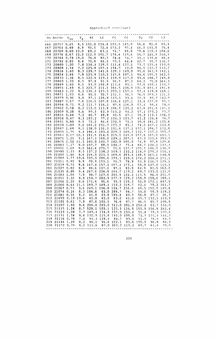
Appnndix-Q rnntfwunl:41.--so-—-.-¢¢-p—-c-:—¢—p:¢q¢-n—n————p—-c-—-qo--—¢_¢o-cc.‘-u-un-—.¢q—-o———¢:—¢

do Rncfln Hsw T2 81 L1 C1 C1 T, "2 12166 20757 0.65 8.3 131 0 134 4 103.5 145.8 56.4 81.4 65.4167 20764 0.48 8.9 80 0 72.4 173.2 90.4 44.3 143.0 79.4168 20768 0.60 10.0 69.3 63.1 4.7 66.8 70.6 110.3 104.6169 20776 0.67 10.0 112.0 101 7 178.6 110.6 35.7 340.9 210.7170 20784 0.78 10.0 76 0 90 7 74.6 74.7 30.1 138.6 86.4171 20792 0.85 9.4 75.8 94.3 70.5 64.4 42.7 98.7 136.7172 20800 1.00 7.8 134.4 128.5 111.6 137.1 73.0 125.4 110.0173 20808 1.34 7.2 125.8 107.4 184.0 12.0 84.0 142.2 142.7174 20816 1.60 8.3 129.7 141.5 128.3 140.9 95.6 163.9 142.1175 20824 1346 7.9 123.9 110.2 145.6 107.5 94.6 195.3 162.5176 20832 1.36 8.5 122 6 110.1 119.9 117.8 99.6 106.7 145.8177 20840 1.20 8.3 87 9 91.9 96.8 87.2 64.2 75.0 164.3178 20848 1.60 8.5 93 0 104.8 113.6 93.1 82.6 140.1 153.7179 20855 1.48 8.3 223 7 211.1 364.5 236.0 131.9 403 4 181.8180 20863 1.22 9.2 136.3 137.5 202.3 157.4 87.4 118.8 168.1181 20871 1.03 8.6 90.5 90.7 103.3 98.3 76.5 789.3 121.2182 20879 0.96 9.0 97.1 126.9 140.5 93.6 56.9 90.7 142.9183 20887 0.67 7.6 116 5 107.8 336.4 127.1 33.4 427.0 89.5184 20894 0.71 8.2 111 7 116.3 97.6 116.8 57.4 98.4 79.8185 20902 0.58 8.2 119.0 113.8 106.8 130.2 67.8 281.5 145.3186 20909 0.38 8.6 90.3 63.9 115.2 84.2 57.1 373.2 73.7187 20916 0.44 7.2 46.7 49.9 43.5 47.1 55.2 112.1 104.2188 20924 0.47 8.3 103.2 77.2 104.3 103.7 41.2 124.4 74.7189 20931 0.80 9.0 72.2 4.6 102.9 73.1 4 .6 241 2 125.6190 20939 1909 8.6 101.2 101.7 103.3 85.3 74.0 417.1 142.8191 20947 1.48 8.1 138 0 131.3 191.6 137.1 107 1 286.7 172.8192 20955 1.75 9.4 186 1 193.4 220.3 140.2 132.7 237.1 305.7193 20963 2.17 10.3 191 5 214.5 219.0 149.8 187.6 165.8 403 5194 20971 1.25 9.1 167 3 168.0 129.1 207.5 63.9 333.6 283.7195 20975 1.50 11.3 109 0 103.7 142.9 105.0 74.9 87.8 129.6196 20983 1. 7 9.0 107.7 88.0 104.7 75.4 66.7 124.1 137.3197 20901 1.68 9.5 362.4 270.7 85.6 127.7 100.2 104.0 136.8198 20995 1.33 9.5 137.2 138.2 149.5 132.2 114.0 170.2 156.3199 21000 1.46 9.6 216.0 223.3 168.6 283.4 149.5 163.1 149.8200 21008 1.77 10.6 235.3 206.6 188.3 239.5 174.2 204.4 251.1201 21011 0.90 9.8 80.8 153.1 84.0 79.9 53.9 146.2 129.1202 21019 0.71 8.6 147.4 157.1 107.4 173.1 55.8 127.0 110.9203 21027 0.82 9.9 99.6 137.1 97.1 83.9 64.9 93.5 162.2204 21035 0.88 9.4 267.6 226.8 164.0 119.2 69.7 133.0 121.8205 21043 1.00 7.9 99.7 117.6 203.8 122.4 115.5 94.4 201.0206 21051 2.32 9.8 159.7 202.9 107.8 129.2 158.8 158.6 180.1207 21056 0.28 8.6 171 6 95.6 99.9 158.3 52.0 173.1 497.9208 21060 0.64 11.5 189 7 148.4 159.2 218.7 42.4 78.2 161.7209 21067 0.53 9.6 240 1 156.0 124.7 256.8 48.5 152.0 145.8210 21074 0.24 8.3 106.6 43.0 288.7 94.7 54.0 58.9 118.2211 21081 0.16 8.2 41.9 23.8 180.4 40.3 56.9 47.1 26.2212 21095 0.19 10.6 41 0 42.0 63.0 41.0 45.0 132.1 110.2213 21101 0.61 7.9 87 6 103.5 76.6 97.7 86.5 80.7 105.5214 21107 1.90 9.6 206 4 265.0 312.0 201.9 254.4 82.7 434.0215 21115 1.24 8.7 529.1 103.1 125.9 134.8 150.9 156.8 242.4216 21123 1.09 7.7 140.1 134.8 187.0 153.4 51.4 '78.9 100.6217 21131 1.24 9.4 132.9 115.8 143.0 109.0 73.3 135.4 144 7218 21136 0.78 7.0 84.1 128.9 84.7 89.5 51.9 76.8 64 3219 21144 1.28 8.2 90.1 95.6 222.1 83.6 100.0 86.9 94.2220 21152 0.79 8.1 111.6 87.0 263.2 110.3 60.7 61.4 70.0a-1-o-¢.—¢¢-occoqnccq-o9-Q-1--gun:-n—an:¢-¢—--o¢¢¢¢—--n—¢—n-o¢-——¢q--—o-—c._ on-——.¢

Appendix-B Continual¢sqcu-cccan¢-Q-<a———-qqu-3-o—o—o::c¢¢u-nncoc3—--—c-—--—c—cg.-—o¢c-p¢—--.-9-n-¢_—

no Ihécuca 115w T7 R1 L1 C1 01 T{ C2 12221 21159 0 56 7.9 74.1 92.1 103.3 77.5 33.7 222.9 129.5222 21165 0 28 7.0 46.6 46.4 426.6 47.1 61.3 61.8 61.6223 21173 0.28 9.3 142 1 96.1 66.3 141.0 66.2 124.0 119.0224 21181 0 66 7.8 101 7 80.9 66.4 96.3 36.9 119.2 80.7225 21184 1 36 8.1 95.3 141.7 123.9 100.9 82.2 52.4 209.3226 21192 1 45 8.1 172.5 151.7 187.2 195.6 90.5 130.4 119.6227 21200 1 42 7.4 211.9 105 6 144.1 121.7 86.6 98.3 151.6228 21207 0 93 6.5 106 4 113.2 115.3 97.4 46.0 119.1 95.9229 21215 0 84 619 81 4 90.5 101.2 76.2 43.4 297.0 125.5230 21224 0.83 7.1 87.5 134.4 81.6 89.7 79.1 104.2 92.6231 21231 0.52 7.2 73 3 96.8 187.7 79.2 42.4 91.5 65.5232 21238 1.42 9.9 164.5 146.2 150.3 132.9 98.2 125.8 183.4233 21246 1.19 10.4 153.2 109 0 174.4 131.0 99.8 163.3 127.6234 21248 0.75 10.4 100 3 104.2 113.8 82.9 36.4 120.6 97.4236 21256 0.44 9.1 100.1 69.4 71.1 100.9 41.4 123.4 59.6236 21262 0.47 12.4 137.6 155.0 139.7 153.5 87.0 99.7 91.8237 21270 0 36 12.7 145 3 80.7 103.6 157.6 32.4 52.6 160.1238 21276 0 29 12.1 40 7 45.2 67.4 43.7 38.1 194.7 125.6239 21284 0 36 12.4 58.9 63.0 139.5 58.7 45.5 49.4 97.5240 21290 0 21 11.0 88 4 53.6 63.3 96.3 40.0 109.6 102.2211 21297 0 28 7.7 363.8 137.7 87.8 331.4 56.2 159.9 245.4242 21305 0.17 9.9 40.5 25.9 49.8 43.6 45.0 32.0 74.2713 21320 0.20 12.1 34.9 27.6 46.2 37.0 38.0 39.9 118.7244 21326 0.30 10.8 170.3 124.3 143.9 75.0 36.6 129.8 160.6245 21334 0.40 12.7 70.6 51.8 80.5 71.2 29.2 52.2 95.7246 21338 0.32 13.0 37.2 46.1 64.9 35.6 37.8 41.1 37.1247 21360 0.43 13.0 73.2 74.1 4 .9 79.1 31.2 67.3 134.6248 21368 0.39 13.0 69 6 112.4 52.1 67.4 34.0 73.7 129.6249 21366 0.24 13.7 59 2 36 2 96.7 60.5 36.0 34.8 99.2250 21373 0.34 55.4 41 9 31.2 55.0 15.0 119.0 87.0251 21381 0.29 11.8 42.3 56.4 41.3 41.7 38.8 34.2 162.4252 21389 0.28 12.7 40 0 49.9 4.1 39.7 37.9 62.0 262.7253 21397 0.51 11.8 70 3 77.5 136.4 67.6 26.1 118.8 117.7254 21405 0.65 11.5 63 7 67.9 159.2 65.7 38.4 115.9 129.5255 21413 0.69 11.8 125.0 104.3 101.8 138.3 44.9 207.4 155.9266 21421 0.68 12.1 66.3 118.2 67.2 61.6 46.6 109.7 297.1257 21429 0.59 11.5 90.7 80.0 92.7 91.0 37.9 83.3 158.8258 21437 0.42 10.6 69.4 70.7 81.5 67.2 34.5 206.3 113.0259 21444 0.47 9.8 215.7 103.0 266.3 200.9 36.6 424.5 175.5260 21451 0 54 11.5 59.2 55.7 60.1 57.6 26.3 72.0 134.2261 21456 0 58 10.4 97 6 107.6 125.4 94.2 45.6 123.3 173.3262 21457 0.84_ 8.6 64.2 91.7 46.3 58.9 46.4 73.5 133.6263 21459 0.56 8.6 52 7 S7 7 34.4 50.8 29.9 26.4 76.4264 21466 0 43 8.5 55 7 58.4 49.3 57.0 44.2 195.6" 58.8265 21473 0.41 8.9 91 5 93.2 116.2 92.5 44.8 111.1 90.3266 21476 0 32 9.4 72 9 67.6 117.9 69.6 4 .2 371.0 106.2267 21484 0 34 _8.6 144.2 123.0 113.8 141.5 50.5 117.2 171.8268 21492 0.26 ,8.5 197.7 137.8 163.3 176.5 58.0 119.8 137.2269 21500 0.27 10.4 100.4 45.3 54.7 95.2 45.0 128.1_ 70.7270 21507 0.36 6.7 67.8 62.4 101.5 67.6 62.5 500.6 67.0271 21514 0.22 7.7 109 8 60.1 493.4 106.1 66.0 236.4 37.1272 21522 0 17 9.5 97.3 34.0 57.5 92.0 63.0 79.5 73.8273 21530 0.14 7.5 87 5 51.5 187.1 83.2 66.0 353.1 81.0274 21537 0 18 7.6 40 0 41.6 342.8 42.2 63.9 835.1 29.4276 21546 0 21 10.1 78 7 39.9 493.9 73.2 49.0 54;! 40.6xxxq-¢—cc-9c-n—o¢¢-—.¢:::::¢¢—--at-—-¢q¢¢—--c:-nun-——-c¢—¢c--acc———¢--49:

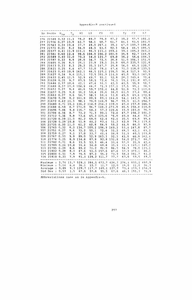
Appendix-8 confiinwnd-¢———--—¢-.¢..—.¢o—o¢¢-o¢n¢c.o—.---4ac-3-¢c-——-¢—¢—--oaa goo--¢c—.—-cc-n-_.¢—_—-p

10 Rncfio H,‘ T7 R1 [1 F1 01 7/ 02 17276 21548 0.32 11.3 78 2 89.7 78 9 97.2 38.2 87.5 101.1277 21556 0.27 10.8 62 7 58.1 68 7 61.7 44.3 83.6 103.0278 21563 0.24 10.4 37.7 48.0 267 1 39.3 47.0 100.7 106.6279 21571 0.21 8.2 84 0 48.3 63.6 82.3 58.4 44.5 105.5280 21577 0.41 11.9 111 1 86.3 111.1 109.4 39.1 105.2 243.2281 21581 0.60 12.4 99.6 104.0 104.2 103.0 35.8 82.7 144.9282 21589 0.40 11.0 70.2 54.0 121.7 69.0 36.2 56.6_104.3283 21597 0.22 9.8 28 0 34.7 73 5 28.8 51.0 306.3 151.0284 21605 0.26 8.5 26.1 23.9 39 5 24.9 68.0 235.5 121.8285 21613 0.23 8.3 29.2 35.3 147.7 28.8 56.0 65.5 120.7286 21621 0.25 6.6 47.7 53.0 79 1 47.4 71.0 118.0 139.5287 21623 0.40 10.8 162.1 66.5 110 1 158.0 36.4 317.9 93.9288 21627 0.34 9.6 115.1 72.5 331.9 114.9 45.8 83.5 147.9289 21632 0.45 11.5 52.9 49.7 55 1 52.8 28.2 749.6 70.4290 21639 0.35 9.7 80.5 58.5 72 6 76.3 55.1 181.8 82.0291 21646 0.37-10.6 4 .1 47.4 51 5 4 .3 40.5 55.9 58.770? 21648 0.37 10.8 104.9 46.8 71.9 107.3 37.5 95.1 78.9293 21651 0.27 9.4 46.6 59.7 103.4 44.8 51.9 73.2 112.0294 21657 0.25 9.8 36.2 59.4 26.6 36.0 61.0 22.4 80.4295 21663 0.27 9.6 54.7 58.3 59.4 53.8 49.0 69.6 172.9296 21670 0.28 8.2 161.9 88.9 80.1 164.8 54.1 142.9 93.9297 21672 0.42 11.3 98.1 70.0 44.9 _96.7 50.3 11.0 194.7298 21680 0.71 10.1 136.2 114.8 254.2 138.0 40.4 157.8 166.5299 21688 0.59 8.7 171.0 96.7 149.2.173.9 46.5 154.4 110.0300 21696 0.46 9.4 116.7 64.3 57.2 124.6 33.9 103.0 76.9301 21704 0.36 8.7 73.2 71.3 90 1 72.4 47.7 104.2 101.2302 21712 0.36 9.9 72.6 65.3 125 6 76.0 40.9 44.4 70.7303 21720 0.39 11.0 81.2 69.0 62 4 82.4 30.5 69.8 99.4304 21728 0.29 10.8 51.9 44.2 82 4 51.2 42.9 79.1 119.6305 21735 0.30 11.0 61.2 60.8 84.8 59.2 44.8 84.0 97.9306 21743 0.32 8.3 134.7 100.1 106.9 149.3 53.4 147.8' 97.7307 21751 0.27 9.6 33.2 50.1 72.4 33.2 48.2 62.1 63.2308 21759 0.27 9.1 37.0 33.7 41 4 34.8 51.9 40.5 109.8309 21767 0.33 9.9 89.0 52.9 160 3 92.3 43.8 60.9 162.4310 21774 0.25 8.9 134.8 87.9 92 8 131.8 54.0 273.7 86.7311 21782 0.21 8.6 33.5 53.3 46 4 33.4 57.0 35.9 42.631? 71789 0.2610.8 36.4 34.0 68 8 35.9 4 .9140.1 148.2313 21795 0.29 8.6 89.2 71.2 81 0 86.0 94.9 79.0 125 1314 21802 0.28 8.3 47.6 51.5 157 6 47.6 57.9 373.1 46.1315 21804 0.31 7.8 75.5 87.3 55 2 73.9 58.2 381.7 93.2116 21810 0.23 7.9 81.4 128.2 311 7 77.7 62.0 59.5 48.3Maximum 2 74 13.7 529.1 384.5 672 7 426.7 276.4 835 1 497.0Mirwimum : 0 14 6.4 26.1 12.7 11 7 12.0 15.0 11 0 26 2Average : 0.89 9.3 129.7 117.7 148 1 127.7 73.1 15 3 156.8Std Dev ° 0.59 1.5 67.6 57.6 95 5 67.6 46.3 15 3 74.9——out-1:-o:c—¢——-—¢¢.--o:¢-¢:oa-q:¢:c¢-n-n-n.—¢qp:-cc-n-¢<-..——.g--n‘-p--——¢——Abbreviations same as in Appendix-A.

207

Appendix-C

PUBLICATIONS OF THE AUTHOR IN THE RELATED FIELDS

waves and their refraction in relation tobeach erosion along the Kerala coast. Centre for EarthScience Studies, Tech. Rep. No. 29, 1983. (M. Baba,N.P. Kurian, K.V. Thomas, M. Prasannakumar, T.S.Shahul Hameed and C.M. Harish).

Study of

Study of waves and their refraction in relation tobeach erosion along the Kerala coast. Centre for EarthScience Studies, Tech. Rep. No. 31, 1983. (M. Baba,P.S. Joseph, N.P. Kurian, K.V. Thomas, T.S. ShahulHameed, M. Prasannakumar and C.M. Harish)

Beach dynamics in relation to wave climate at Alleppeyduring monsoon season. Centre for Earth ScienceStudies, Tech. Rep. No. 38, 1984. (N.P. Kurian, T.S.Shahul Hameed and M. Baba)

Prediction of nearshore wave heights using a refractionprogramme. Coastal Engng., Vol.9, pp.347—356, 1985.(N.P. Kurian,.M. Baba and T.S. Shahul Hameed)

A study of monsoonal beach processes around Alleppey,Kerala. Proc. Indian Acad. Sci. (Earth. Planet. Sci.),Vol.94, pp.323-332, 1985. (N.P. Kurian, T.S. ShahulHameed and M. Baba)

Wave climatology for the southwest coast of India.Paper presented at the Int. Symp. on Concepts andTechniques of Applied Climatology, Waltair, 1985. (M.Baba, T.S. Shahul Hameed, N.P. Kurian, K.V. Thomas,P.S. Joseph, C.M. Harish, M. Prasannakumar and K.K.Varghese)

Impact of a permeable structure on shorelinedevelopment. In: B.P. Radhakrishna and K.K.Ramachandran (Ed.), India's Environment, GeologicalSociety of India, Bangalore, pp.275—288, 1986. (T.S.Shahul Hameed, N.P. Kurian and M. Baba)

Computation of longshore currents. Indian J. Mar. Sci.,Vol.15, pp.92-95, 1986. (T.S. Shahul Hameed, M. Babaand K.V. Thomas)

Beach modification due to alongshore and offshoretransport. Proc.(abstracts) 20th Int. Conf. on CoastalEngng., Taiwan, pp.322—323, 1986. (M. Baba, T.S. ShahulHameed and K.V. Thomas)

208

10.

ll.

12.

13.

14.

15.

Discussion on ‘Mathematical prediction of long-termshoreline changes at Visakhapatnam'. J. InstitutionEngrs. (India), Civil Engng. Div., Vol.67, pp.68, 1986.(M. Baba and T.S. Shahul Hameed)

Temporal and spatial variations in wave climate offKerala. Indian J. Mar. Sci., Vol.16, pp.5-8, 1987. (M.Baba, N.P. Kurian, T.S. Shahul Hameed, K.V. Thomas andC.M. Harish)

Monitoring of coastal environment for its management.Proc. Coastal Zone—87, WW Div., ASCE, Seattle, pp.4764—4777, 1987. (M. Baba, N.P. Kurian, K.V. Thomas, T.S.Shahul Hameed and C.M. Harish)

Prediction system for waves and related coastalprocesses. Paper presented in the 19th GeneralAssembly, IUGG, Vancouver, Canada, 1987. (N.P. Kurian,P.S. Joseph, T.S. Shahul Hameed and K.V. Thomas)

Wave climate and power off Trivandrum. In: Projectreport on sea trial of a 150 kw wave energy device offTrivandrum coast. Published by IIT, Madras on behalf ofDept. of Ocean Development, Govt. of India, 1987. (M.Baba, K.V. Thomas, T.S. Shahul Hameed, N.P. Kurian,C.E. Rachel, Saji Abraham and Ramesh Kumar)

Prediction of sediment transport and beach evolution.In: Ocean Waves and Beach Processes (Ed. M.Baba andN.P. Kurian), Centre for Earth Science Studies,Trivandrum, pp.205-224, 1988. (M. Baba, T.S. ShahulHameed and K.V. Thomas)

209