Spector: An OpenCL FPGA Benchmark Suite

Quentin Gautier, Alric Althoff, Pingfan Meng and Ryan KastnerUniversity of California, San Diego

Abstract—High-level synthesis tools allow programmers touse OpenCL to create FPGA designs. Unfortunately, these toolshave a complex compilation process that can take several hoursto synthesize a single design. This creates a significant barrierfor design optimization since even experts typically need to testmany designs due to the non-obvious interactions between thedifferent optimizations. Thus, understanding the design space,and guiding the optimization process is a crucial requirement forenabling the widespread adoption of these high-level synthesistools. However this requires a significant amount of design spacedata that is currently unavailable or difficult to generate. Tosolve this problem, we present an OpenCL FPGA benchmarksuite. We outfitted each benchmark with a range of optimizationparameters (or knobs), compiled over 8300 unique designs usingthe Altera OpenCL SDK, executed them on a Terasic DE5 board,and recorded their corresponding performance and utilizationcharacteristics. We describe the resulting design spaces, and per-form a statistical analysis of the optimization configurations whichprovides valuable architecture insights to FPGA developers. Wemake the benchmarks and results completely open-source to giveopportunities for the community to perform additional analysesand provide a repository of well-documented designs for follow-onresearch.

I. INTRODUCTION

FPGA design was traditionally relegated to only experi-enced hardware designers, and required specifying the applica-tion using low-level hardware design languages. This providesopportunities to create highly specialized custom architectures;yet it is time consuming as every minute detail must bespecified on a cycle-by-cycle basis. Recently, FPGA vendorshave released high-level synthesis tools centered around theOpenCL programming model. The tools directly synthesizeOpenCL kernels to programmable logic creating a customhardware accelerator. They raise the level of abstraction of theprogramming model and increase the designer’s productivity.Furthermore, the tools manage the transfer of data betweenthe FPGA and the CPU host. This opens the door for moreprogrammers to easily utilize FPGAs.

OpenCL is a open standard that provides a framework forprogramming heterogenous systems. The language extends Cwith features that specify different levels of parallelism anddefine a memory hierarchy. There exists OpenCL implementa-tions for a variety of multicore CPUs, DSPs, and GPUs. Morerecently, commercial tools like Xilinx SDAccel [1] and theAltera OpenCL SDK [2] add FPGAs into the mix of supportedOpenCL devices. This greatly simplifies the integration ofFPGAs into heterogeneous systems, and provides a FPGAdesign entry point for a larger audience of programmers.

The OpenCL FPGA design process starts with implement-ing the application using OpenCL semantics. The designerthen typically employs some combination of well-known

optimizations (e.g. SIMD vectors, loop unrolling, etc.) andsettles on a small set of designs that are considered optimalaccording to some metric of performance (resource utilization,power, etc.). Most designers will need multiple attempts withseveral optimization options to understand the design space.Unfortunately, a major drawback of these OpenCL FPGA toolsis that the compilation time is long; it can take hours or evendays. This severely limits the ability to perform a large scaledesign space exploration, and requires techniques to efficientlyguide the designer to a good solution.

In many applications, it is difficult to predict the perfor-mance and area results, especially when optimization param-eters interact with each other in unforeseen manners. As anexample, increasing the number of compute units duplicatesthe OpenCL kernel, which should improve performance at theexpense of FPGA resources. However, this is not always trueas memory contention may limit the application’s performance.Finding when this occurs requires a better understanding of thememory access patterns and how other optimizations alter it.Many other optimizations are also intertwined in non-intuitiveways as we describe throughout the paper.

We propose an OpenCL FPGA benchmark suite. Eachbenchmark is tunable by changing a set of knobs that modifythe resulting FPGA design. We compiled over 8000 designsacross 9 unique benchmarks using the Altera OpenCL SDK.All of our results are openly available and easily accessible [3].This provides large set of designs to enable research on system-level synthesis for FPGAs. For example, researchers can useour results to evaluate their methods for improving the processof design space exploration. We provide our own analysisof the data as an example use-case in Section V; there issubstantial follow-on work that can be done, and we encourageother researchers to use and extend our results.

The major contributions are:

• Designing and releasing an OpenCL FPGA bench-mark suite

• Creating an optimization space for each benchmarkand describing the parameters that define it.

• Performing a comprehensive set of end-to-end syn-thesis experiments, the result of which is over twentythousands hours of compilation time.

• Providing a statistical analysis on the results to giveinsights on OpenCL FPGA design space exploration.

The remainder of the paper is organized as follows. InSection II, we motivate the need for this research, and dis-cuss related work. In Section III we detail our benchmarkdesign process and talk about how we obtained the results.In Section IV we describe the benchmarks, detail the tunable

978-1-5090-5602-6/16/$31.00 c© 2016 IEEE

Fig. 1. Our workflow to generate each benchmark and then generate the design space results as presented in Section III.

knobs and their effect on the architectures, and present theirdesign spaces. We give a statistical analysis of some of theresults in Section V and conclude in Section VI.

II. MOTIVATION

There are substantial number of application case studies forparallel computing, heterogeneous computing, and hardwaredesign. One can start with reference designs from hardwarevendors such as Intel, NVIDIA, Altera, and Xilinx. Unfor-tunately, these are often scattered across different websites,use different target compute platforms (CPU, GPU, FPGA),and they lack a common lingua franca in terms of opti-mization parameters. This makes them difficult to provide afair comparison across the different applications. This is thegeneral motivation for benchmark suites – they provide highlyavailable, well documented, representative set of applicationsthat can assess the effectiveness of different design strategiesand optimizations.

Several open-source benchmarks for parallel applicationscurrently exist. Many of these, e.g., the HPEC challengebenchmark suite [4] or Rodinia [5], focus on GPUs andmulticore CPUs. FPGAs have a different compute model.Thus, while some of the applications in these benchmarkssuites are applicable to studying the OpenCL to FPGA designflow, they require modifications to be useful. Several of ourbenchmarks are found in these existing benchmark suites.There are also a number of FPGA specific benchmarks suites.These generally target different parts of the design flow. Forexample, the applications in ERCBench [6] are written inVerilog and useful for studying RTL optimizations or as acomparison point for hardware/software partitioning. Titan [7]uses a customized workflow to create benchmarks to studyFPGA architecture and CAD tools. The OpenCL dwarfs [8],[9] contain several OpenCL programs that have been optimizedfor FPGA. Unfortunately, they usually have a fixed architecturewith little to no optimization parameters.

We seek to extend these benchmark suites by leveragingthe existing OpenCL benchmarks and reference programs, andoutfitting them with multiple optimization parameters. Each ofthese designs can be compiled with a commercial program oropen-source tool to generate thousands of unique configura-tions. We make open-source our results that we obtained fromthe Altera software, and encourage the community to compileour benchmarks with different tools. One of our motivatingfactors in creating this benchmark suite was the lack of a com-mon set of designs and optimization parameters for comparingdifferent design space exploration (DSE) techniques. Machinelearning techniques for DSE in particular can benefit from alarge set of designs, e.g., [10] and [11] use machine learning

TABLE I. NUMBER OF SUCCESSFULLY COMPILED DESIGNS.

BFS 507 Histogram 894 Normal estimation 696DCT 211 Matrix Multiply 1180 Sobel filter 1381FIR filter 1173 Merge sort 1532 SPMV 740

approaches to explore design spaces and predict the set ofPareto designs without having to compile the entire space.These techniques could directly leverage our results to verifyand perhaps improve their models. And in general, we believethat open repository of OpenCL FPGA designs will benefitthis and other areas of research.

III. METHODOLOGY

We designed nine benchmarks that cover a wide rangeof applications. We selected benchmarks that are recurrentin FPGA accelerated applications (FIR filter, matrix multiply,etc.), but we also included code with more specific purpose tocover potential real-world programs (like histogram calculationand 3D normal estimation). These benchmarks come fromvarious places: some were written directly without examplesource code, others come from GPU examples, and some comefrom FPGA optimized examples. In all cases, we started fromprograms that contained little to no optimization parameters,thus requiring us to define the optimization space.

For each benchmark, we proceeded as illustrated inFigure 1. First we created or obtained code that was partiallyor fully optimized for FPGA. It is important to note thatwe were not trying to reach a single “most optimal” design,but instead defining an optimization space that covers a widerange of optimizations. We studied which types of optimizationwould be relevant for each benchmark. Then we added severaloptimization knobs, which are values that we can tune atcompile-time. These knobs can enable or disable code, oraffect an optimization parameter (e.g., unrolling factor). Wecompiled several sample designs to ensure that the knobs wehad chosen would have some impact on the timing and area.Each benchmark has a set of scripts to generate hundreds ofunique designs, with all the possible combinations of knobvalues. In most cases we restricted the values of the knobs toa subset of the options (e.g., powers of two). We also removedvalues that were likely to use more resources than available,and filtered out further using pre-place-and-route estimations.All the benchmarks were written using standard OpenCL codewith a C++ host program that can run and measure the time ofexecution. The OpenCL code works with the Altera SDK forFPGA, and can also be executed on GPU and CPU. Althoughwe have not tested the programs with other commercial oropen-source OpenCL-to-FPGA pipelines, we expect that littleto no modifications are required to ensure compatibility.

Normalized Throughput0 0.2 0.4 0.6 0.8 1

Norm

aliz

ed 1

/Logic

utiliz

ation

0.2

0.4

0.6

0.8

1

BFS dense

Normalized Throughput0 0.2 0.4 0.6 0.8 1

Norm

aliz

ed 1

/Logic

utiliz

ation

0.2

0.4

0.6

0.8

1

BFS sparse

Fig. 2. BFS design spaces for dense and sparse inputs. We plot the inverselogic utilization against the throughput such that higher values are better. ThePareto designs are shown in red triangles.

Each design was then individually compiled using theAltera OpenCL SDK v14.1, with a compile time typicallyrequiring 1 to 4 hours on a modern server, and occasionallytaking more than 5 hours per design. In total we successfullycompiled more than 8300 designs (see Table I), plus manymore that went through almost the entire compilation processbut failed due to device resource limits. We executed thesuccessful designs on a Terasic DE5 board with a Stratix VFPGA to measure the running time for a fixed input. Someapplications can behave differently given a different set ofinput data however, and the optimizations to use in these casesmight vary. This is the case for algorithms like graph traversalor sparse matrix multiplication, where the sparsity of the inputcan have a significant impact on the design space. In both ofthese benchmarks we ran the program with two sets of inputs.We ran BFS with both a densely connected graph and onewith sparse edges. Sparse matrix-vector multiplication was runwith one matrix containing 0.5% of non-zero values and oneonly 50% sparse. We extracted the running time and area data(such as logic, block RAM, DSPs, etc.) for each run. The setof design spaces that we present in Figures 2 to 8 shows thelogic utilization against the running time, as logic is usually themost important resource and often the limiting factor. Theseresults are generated from the scripts plot_design_space.mand plot_all_DS.m available in our repository.

IV. BENCHMARKS DESCRIPTION

Here we describe the benchmarks and the knobs that wehave chosen, so that the reader can interpret the design spaceresults based on the design choices. First we explain someof the most common optimization types in OpenCL designs.Then we explain each benchmark in more details, followed byan overview of the shape of the design space.

Work-items: These are parallel threads with a commoncontext on GPU. On FPGA, they can be interpreted as multipleiterations of an outer loop that is pipelined by the compiler.Using only one can give more flexibility to the programmerto control unrolling and pipelining, while using multiple canenable optimizations such as SIMD. Work-groups: This de-fines how many groups of work-items to use, each groupusing a different context (no shared memory). This is useful toenable the compute units optimization. Compute units: Howmany duplicates of the kernel are created on the FPGA chip.Compute units can run work-groups in parallel, however theyall access the external memory and thus might be limited bythe bandwidth. SIMD: Work-items can be processed simul-

taneously by increasing local area usage. It is only possiblewhen there is no branching. Unrolling: By explicitly unrollinga loop, we can process multiple elements simultaneously byusing more area, usually storing data in more local registers.

A. Breadth-First Search (BFS)

This code is based on the BFS FPGA benchmark fromthe OpenDwarfs project [8], [9], and originally based on theBFS benchmark from the Rodinia Benchmark Suite [5]. It isan iterative algorithm that simply traverses a graph starting ata specified node by performing a breadth-first traversal, andreturns a depth value for each node. The algorithm iteratesover two OpenCL kernels until all the reachable nodes havebeen visited. Each kernel launches work-items for each nodein the graph and uses binary masks to enable computation.There are 6 knobs with varying values in these kernels.

• Unroll factor in kernel 1: Unrolls a loop to processmultiple edges simultaneously. We enable additionalcode for edge cases only if the unroll factor is greaterthan 1.

• Compute units in kernel 1 and 2, SIMD in kernel 2.• Enable branch in kernel 1: Describes how to check

if a node was visited and how to update graph maskvalues. Either enables the code from OpenDwarfs withbitwise operators to avoid branching, or enables thecode from Rodinia with regular if statement.

• Mask type: Number of bits used to encode the valuesof graph masks.

Design space: (Figure 2) The design space for the denseinput is clearly divided along the timing axis. The left clusterrepresents the designs where the branching code is disabled.The more optimized branching code gets better performanceas we increase the unrolling factor. The discontinuity betweenthe middle and right clusters is caused by a jump in the knobvalues. The impact of the unrolling factor is however limitedby the number of edges to process per node. This limitation isreflected in the sparse input design space that is more uniform.

B. Discrete Cosine Transform (DCT)

This algorithm is based on the NVIDIA CUDA imple-mentation of a 2D 8x8 DCT [12]. The program divides theinput signal into 8x8 blocks loaded into shared memory, thenprocessed by calculating DCT for rows then columns withprecalculated coefficients. Some knobs enable multiple blocksto be loaded in shared memory, and multiple rows and columnsto be processed simultaneously. Each work-group processesone 8x8 block, and within the group each work-item processesone row and column. This can be altered by 9 tunable knobs:

• SIMD and Compute units.• Block size: Number of rows/columns to process per

work-item.• Block dim. X and Block dim. Y: Number of blocks

per work-group in X or Y direction.• Manual SIMD type: Using OpenCL vector types,

each work-item processes either multiple consecutiverows/columns, or processes multiple rows/columnsfrom different blocks.

Normalized Throughput0 0.2 0.4 0.6 0.8 1

Norm

aliz

ed 1

/Logic

utiliz

ation

0.2

0.4

0.6

0.8

1

DCT

Normalized Throughput0 0.2 0.4 0.6 0.8 1

Norm

aliz

ed 1

/Logic

utiliz

ation

0.2

0.4

0.6

0.8

1

FIR filter

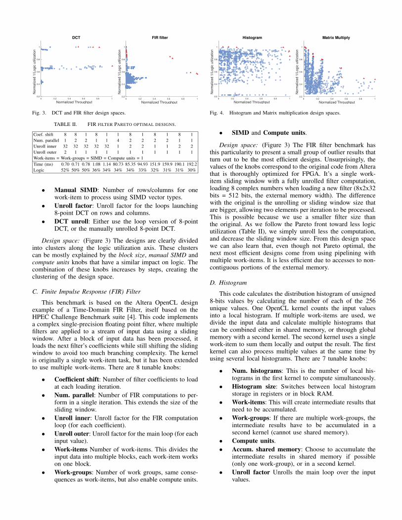
Fig. 3. DCT and FIR filter design spaces.

TABLE II. FIR FILTER PARETO OPTIMAL DESIGNS.

Coef. shift 8 8 1 8 1 1 8 1 8 1 8 1Num. parallel 1 2 2 1 1 4 2 2 2 2 1 1Unroll inner 32 32 32 32 32 1 2 2 1 1 2 2Unroll outer 2 1 1 1 1 1 1 1 1 1 1 1Work-items = Work-groups = SIMD = Compute units = 1Time (ms) 0.70 0.71 0.78 1.08 1.14 80.73 85.35 94.93 151.9 159.9 190.1 192.2Logic 52% 50% 50% 36% 34% 34% 34% 33% 32% 31% 31% 30%

• Manual SIMD: Number of rows/columns for onework-item to process using SIMD vector types.

• Unroll factor: Unroll factor for the loops launching8-point DCT on rows and columns.

• DCT unroll: Either use the loop version of 8-pointDCT, or the manually unrolled 8-point DCT.

Design space: (Figure 3) The designs are clearly dividedinto clusters along the logic utilization axis. These clusterscan be mostly explained by the block size, manual SIMD andcompute units knobs that have a similar impact on logic. Thecombination of these knobs increases by steps, creating theclustering of the design space.

C. Finite Impulse Response (FIR) Filter

This benchmark is based on the Altera OpenCL designexample of a Time-Domain FIR Filter, itself based on theHPEC Challenge Benchmark suite [4]. This code implementsa complex single-precision floating point filter, where multiplefilters are applied to a stream of input data using a slidingwindow. After a block of input data has been processed, itloads the next filter’s coefficients while still shifting the slidingwindow to avoid too much branching complexity. The kernelis originally a single work-item task, but it has been extendedto use multiple work-items. There are 8 tunable knobs:

• Coefficient shift: Number of filter coefficients to loadat each loading iteration.

• Num. parallel: Number of FIR computations to per-form in a single iteration. This extends the size of thesliding window.

• Unroll inner: Unroll factor for the FIR computationloop (for each coefficient).

• Unroll outer: Unroll factor for the main loop (for eachinput value).

• Work-items Number of work-items. This divides theinput data into multiple blocks, each work-item workson one block.

• Work-groups: Number of work groups, same conse-quences as work-items, but also enable compute units.

Normalized Throughput0 0.2 0.4 0.6 0.8 1

Norm

aliz

ed 1

/Logic

utiliz

ation

0.2

0.4

0.6

0.8

1

Histogram

Normalized Throughput0 0.2 0.4 0.6 0.8 1

Norm

aliz

ed 1

/Logic

utiliz

ation

0.2

0.4

0.6

0.8

1

Matrix Multiply

Fig. 4. Histogram and Matrix multiplication design spaces.

• SIMD and Compute units.

Design space: (Figure 3) The FIR filter benchmark hasthis particularity to present a small group of outlier results thatturn out to be the most efficient designs. Unsurprisingly, thevalues of the knobs correspond to the original code from Alterathat is thoroughly optimized for FPGA. It’s a single work-item sliding window with a fully unrolled filter computation,loading 8 complex numbers when loading a new filter (8x2x32bits = 512 bits, the external memory width). The differencewith the original is the unrolling or sliding window size thatare bigger, allowing two elements per iteration to be processed.This is possible because we use a smaller filter size thanthe original. As we follow the Pareto front toward less logicutilization (Table II), we simply unroll less the computation,and decrease the sliding window size. From this design spacewe can also learn that, even though not Pareto optimal, thenext most efficient designs come from using pipelining withmultiple work-items. It is less efficient due to accesses to non-contiguous portions of the external memory.

D. Histogram

This code calculates the distribution histogram of unsigned8-bits values by calculating the number of each of the 256unique values. One OpenCL kernel counts the input valuesinto a local histogram. If multiple work-items are used, wedivide the input data and calculate multiple histograms thatcan be combined either in shared memory, or through globalmemory with a second kernel. The second kernel uses a singlework-item to sum them locally and output the result. The firstkernel can also process multiple values at the same time byusing several local histograms. There are 7 tunable knobs:

• Num. histograms: This is the number of local his-tograms in the first kernel to compute simultaneously.

• Histogram size: Switches between local histogramstorage in registers or in block RAM.

• Work-items: This will create intermediate results thatneed to be accumulated.

• Work-groups: If there are multiple work-groups, theintermediate results have to be accumulated in asecond kernel (cannot use shared memory).

• Compute units.• Accum. shared memory: Choose to accumulate the

intermediate results in shared memory if possible(only one work-group), or in a second kernel.

• Unroll factor Unrolls the main loop over the inputvalues.

Normalized Throughput0 0.2 0.4 0.6 0.8 1

Norm

aliz

ed 1

/Logic

utiliz

ation

0.2

0.4

0.6

0.8

1

Merge Sort

Normalized Throughput0 0.2 0.4 0.6 0.8 1

Norm

aliz

ed 1

/Logic

utiliz

ation

0.2

0.4

0.6

0.8

1

Normal estimation

Fig. 5. Merge sort and Normal estimation design spaces.

Design space: (Figure 4) This is one of the few designspaces that appear relatively uniform. All the knobs seemto have a similar impact on the variations between designs,although a few design make the exception by using more logic.These designs set the histogram size such that the compilerwill prefer to use registers instead of block RAMs, as theyare using only one local histogram. But as opposed to someother uniform design spaces, the parameters cannot be linearlymodeled, as presented in Section V.

E. Matrix Multiplication

This code is based on an Altera OpenCL example. Itimplements a simple matrix multiply C = A∗B with squaredfloating-point matrices. The matrix C is divided into blocks,each computed individually. The implementation includes sev-eral knobs to change the size of the blocks and to processmultiple blocks at once. Each work-group takes care of oneblock of C. Each work-item takes care of one element in ablock, including loading elements to local storage, multiplyingone row of block A by one column of block B, and copyingback to global storage. There are knobs that enable multipleblock processing for work-groups and work-items, either byadding an inner loop, or by using OpenCL vector types forSIMD computation. There are 9 tunable knobs in this code:

• Block dimension: Width of blocks.• Sub-dimension X and Sub-dimension Y: How many

blocks of C in X or Y direction to process in onework-group. This adds a for loop so that each work-item processes this number of blocks.

• Manual SIMD X and Manual SIMD Y: How manyblocks of C in X or Y direction to process in onework-group. This performs the inner matrix multiplywith OpenCL vector types.

• SIMD and Compute units• Enable unroll: Enables or disables unrolling loop on

load and store operations.• Unroll factor: Unroll factor for multiple loops.

Design space: (Figure 4) The matrix multiplication Pareto-optimal designs are a good example of an almost linearrelationship between area and timing (in this optimizationspace). By looking at the knob values along the Pareto front,we can determine that it’s mostly a combination of blockdimension, manual SIMD X, SIMD, and unroll factor thatcan vary the results and create the trade-off between speedand area. The other knobs still have an impact on the designspace, but tend to have a single optimal value for both area and

timing. Typically, manual SIMD Y is not enabled in the optimaldesigns, as the data are organized along the X direction.

F. Merge Sort

This program applies the Merge Sort algorithm using loops,merging in local memory first, then in global memory:

1: for each chunk of size localsortsize do2: copy the entire chunk into local memory3: for localchunksize = 2 to localsortsize do4: for each local chunk of the chunk do5: merge two halves of local chunk6: end for7: swap input/output buffers8: end for9: end for

10: for chunksize from localsortsize to inputsize do11: for each chunk of the input do12: merge two halves of the chunk13: end for14: swap input/output buffers15: end for

• Work-items: Each work-item processes a differentchunk in lines 4 and 11.

• Local sort size: Varies localsortsize.• Local use pointer: Use pointers to swap buffers in

local memory. This can force the use of block RAMsinstead of registers.

• Specialized code: Enable a specialized code to mergechunks of size 2.

• Work-groups: Each work-group runs the algorithmon one portion of the input data. A second iterationof the kernel is launched to merge the final output.

• Compute units• Unroll: Unroll factor for the loops copying data

from/to local memory.

Design space: (Figure 5) This design space is mainlydivided into 2 clusters, due to the compute units knob that cantake the value 1 or 2. In this case, using multiple computeunits has a large impact on the resource utilization, whilethe other knobs have a much smaller impact on resources,and are responsible for smaller variations within each cluster.Interestingly, the fastest designs use only one compute unit,but make use of the pipeline optimization from work-items.

G. 3D Normal Estimation

This code is inspired by an algorithm in the KinectFusioncode from the PCL library [13]. It estimates the 3D normalsfor an organized 3D point cloud that comes from a depth map(vertex map). We can quickly estimate the normals for all thepoints by using the right and bottom neighbors on the 2Dmap, then calculate the cross-product of the difference betweeneach neighbor and the current point, and normalize. If any ofthe vertices is null, the normal is null. One kernel does theentire computation using a small sliding window where theright neighbor is shifted at each iteration to be reused in thenext iteration. As illustrated in Figure 6, a parameter can varythe window size so that multiple inputs are processed in one

x/y/z x/y/z

x/y/z x/y/z

x/y/z

x/y/z

x/y/z

x/y/z

x/y/z

null

null null

x/y/z x/y/z x/y/z x/y/z

✄

✄

�

x/y/zx/y/z

Vertex map Normal map

Sliding window:

Size = 1 Size = 2

Fig. 6. Estimating 3D normals from 3D vertices organized on a 2D map.The top of the figure shows how the sliding window works in the algorithm.The bottom illustrates how the sliding window can be tuned.

iteration. If multiple work-items are used, the input data arecut into blocks of whole rows. There are 6 tunable knobs:

• Work-items, Work-groups and Compute units.• Unroll factor 1: Unroll factor for the outer loop that

iterates over all the input data.• Unroll factor 2: Unroll factor for the loop that iterates

over the elements within a sliding window.• Window size: Size of the sliding window. ie. number

of consecutive elements to process in one iteration.

Design space: (Figure 5) Normal estimation is anotherexample of a fairly uniform design space. It is easier to create amodel of the knobs (see Section V), and it is a good example ofa optimization space where most parameters have an impact ofsimilar importance on both the timing and the area utilization.

H. Sobel Filter

This code applies a Sobel filter on an input RGB image,based on the Altera OpenCL example.

1: for each block on the input image do2: load pixel values from block in shared memory3: for each pixel in local storage do4: load the 8 pixels around from shared memory to

registers5: convert pixels to grayscale6: apply the 3x3 filter in X and Y7: combine the X and Y results and apply threshold8: save result in global storage9: end for

10: end for

Work-group take care of blocks (line 1) and work-itemtake care of pixels within the block (line 3). The knobs canenable a sliding window within the blocks, SIMD computation,or make a work-item perform multiple computations. With theSIMD parameter, each work-item loads more pixels to registersto apply multiple filters by using OpenCL vector types. Thesliding window parameter creates an inner loop (after line 3)where each work-item processes one pixel (or multiple withSIMD), then shifts the registers to load one new row or columnof data from the local storage. There are 8 knobs in this code:

Normalized Throughput0 0.2 0.4 0.6 0.8 1

Norm

aliz

ed 1

/Logic

utiliz

ation

0.2

0.4

0.6

0.8

1

Sobel filter

Fig. 7. Sobel filter design space.

• Block dimension X and Block dimension Y: Size ofeach block in X or Y.

• Sub-dimension X and Sub-dimension Y: Local slid-ing window size, moving in X or Y direction.

• Manual SIMD X and Manual SIMD Y: Number ofelements to process as SIMD in X or Y direction.

• SIMD and Compute units.

Design space: (Figure 7) The Sobel filter is anotherexample of a mostly uniform design space where all the knobsseem to have a similar impact on the output variables. A moredetailed look at the knob values actually shows that along thetiming axis, the manual SIMD X knob is one of the mostimportant factors, and the most important on the Pareto front.This is a case where manually designing SIMD computation isbetter than using automatic SIMD, and this becomes apparentfrom the analysis of an entire optimization space.

I. Sparse Matrix-Vector Multiplication (SPMV)

This code is also based on an OpenDwarfs benchmark. Itcalculates Ax+y where the matrix A is sparse in CSR formatand the vectors x and y are dense. Each work-item processesone row of A to multiply the non-zero elements by elementsof x. Two knobs control the number of elements processedsimultaneously by one work-item: one unrolls a loop, and theother enables the use of OpenCL SIMD vector types to storeand multiply the data. There are 4 tunable knobs:

• Block dimension: Number of work-items per work-group.

• Compute units.• Unroll factor: This creates an inner loop over some

number of elements and unrolls it so that elements canbe processed simultaneously.

• Manual SIMD width: This is the size of the OpenCLvector type to use when processing elements. Elementsare loaded and multiplied in parallel using this type.

Design space: (Figure 8) This benchmark is dependent onthe type of input and behaves differently for more or less sparsematrices. This is reflected in the design spaces, where the mostefficient designs for sparse matrices, and particularly the Paretooptimal designs, tend to have smaller values for Unroll factorand Manual SIMD width. When processing a denser matrix,the best designs tend to have a higher value for these knobs,as it allows simultaneous processing of elements in rows. Forsparse matrices, the pipelining provided by block dimension isusually preferred to the SIMD and unroll optimizations.

Normalized Throughput0 0.2 0.4 0.6 0.8 1

Norm

aliz

ed 1

/Logic

utiliz

ation

0.2

0.4

0.6

0.8

1

SPMV 0.5%

Normalized Throughput0 0.2 0.4 0.6 0.8 1

Norm

aliz

ed 1

/Logic

utiliz

ation

0.2

0.4

0.6

0.8

1

SPMV 50%

Fig. 8. SPMV design spaces for 0.5% sparse matrix and 50% sparse matrix.

V. DESIGN SPACE ANALYSIS

To demonstrate one potential use of our data, we performan example analysis to determine the viability of multiplesparse linear regression to model design space performanceand area. In mathematical form we compute model coefficientsβ in

f(x) = β0 +

n∑i=1

xiβi +

m∑i=n+1

m∑j=i+1

xixjβi·m+j (1)

where x is a vector of design space knob values, n is thenumber of design space knobs, and the number of entries in βis m = n(n+1)/2. In the following sections, we use the term“parameters” to refer to values of β and “realization” to referto a single design (a single point in the design space plots ofprevious sections).

The purpose of this analysis is not to suggest that linearregression is a good idea when seeking to model a design spacein general. Rather we observe that there are many cases wheresimple linear models are effective, and equally many wherethey are misleading and/or downright ridiculous. The lessonhere is that DSE research involving parametric models shouldnot overstate their generality, particularly where performanceis concerned.

A. The Least Absolute Shrinkage and Selection Operator(LASSO)

The LASSO is a well-known statistical operator [14] usefulfor variable selection and sparse modeling. While we presentits mathematical form in equation (2), LASSO is, in essence,ordinary least squares regression with a penalty forcing smallvariables toward zero. The operator parameter λ determines“small”, and it is often—as it is in our case—selected viacross-validation. A small value at βk indicates that variationof the kth parameter does not produce significant variationin the output. We prefer LASSO for this analysis because ittends to produce simpler and more interpretable models. TheLASSO in mathematical form is

minβ‖y −Xβ‖22 + λ‖x‖1 (2)

= minβ

n∑i=1

(yi −m∑j=1

Xijβj)2 + λ

m∑i=1

|βi|

where Xij is the entry of the matrix X at row i and columnj. In the remainder of this section β refers to the vectorminimizing the LASSO for a λ minimizing the model meansquared error.

TABLE III. LASSO r2 AND G(β) VALUES FOR LOGIC (`) AND TIMING(t) ACROSS BENCHMARKS FOR COMPLETE AND NEAR-PARETO SPACES

Complete Space Within 0.1 of ParetoBenchmark r2` G`(β) r2t Gt(β) r2` G`(β) r2t Gt(β)

BFS (Dense) 0.89 0.91 0.97 0.97 0.92 0.85 0.83 0.97BFS (Sparse) 0.89 0.91 0.85 0.84 0.98 0.68 0.92 0.80DCT 0.98 0.83 0.91 0.86 0.58 0.86 0.95 0.86FIR 0.61 0.92 0.37 0.94 0.79 0.95 0.99 0.96Histogram 0.73 0.90 0.04 0.80 -0.05 1.00 0.15 0.94Matrix multiply 0.83 0.76 0.70 0.70 0.91 0.82 0.94 0.71Normal estimation 0.90 0.81 0.91 0.57 0.98 0.72 0.98 0.69Sobel 0.78 0.77 0.88 0.67 0.98 0.83 0.94 0.78SPMV (Sparse) 0.88 0.93 0.29 0.71 0.90 0.89 0.24 0.93SPMV (Dense) 0.88 0.93 0.24 0.82 0.90 0.94 0.68 0.80Mergesort 0.91 0.89 0.43 0.68 0.95 0.92 0.74 0.81

Note: G(β) values for which the associated r2 < 0.7 are greyed out toindicate that they should be disregarded

While LASSO explicitly determines coefficients for a linearmodel, it is also useful for variable selection in nonlinearsystems [15]. In this situation we do not read very deeplyinto β, but rather use it to detect when simple linear, perhapseven obvious, relationships exist between parameters and therealized design space. To summarize the LASSO results wecompute the coefficient of determination—also known as ther2 value—independently for throughput and area, denotedr2t and r2` respectively. r2 is a commonly used goodness-of-fit measure indicating the amount of variance in the dataexplained by the model. Alongside r2t,` we also computethe Gini coefficient of β, Gt,`(β), as a measure of modelcomplexity. Note that if r2 is small then G(β) is a nearlyworthless quantity. We do, however, include values for alldesign spaces in Table III for completeness.

B. Gini Coefficient

The Gini coefficient [16] G is a statistic frequently usedto measure economic inequality. G takes values in the range[0, 1]. If G(v) = 1 − ε for a particular vector v and small ε,then there are a few elements of the set that are very largerelative to others. If G(v) = ε then all vector elements havevalues that are close to each other.

Equation (3) describing G is calculated using equation (3)with bias correction from [17]

G(x) =n

n− 1·∑ni=1(2i− n− 1)xin∑ni=1 xi

(3)

where x is sorted beforehand. G(β) indicates whether variationin the realized design space can be accounted for by a fewparameters.

C. Example observations

To give the reader some idea of the sort of descriptivestatistical information that can be gained from these data, wewill consider only the the r2 and Gini values from Table III forthe Histogram and Normal estimation design spaces. A purelyvisual inspection of the design space graph, (see Figure 5 and 4resp.) might suggest that there is a “grid-like” quality to therelationship between knobs and the realized design space. Wedemonstrate that this is not necessarily the case.

0 100 200 300 400 500 600 700 8000

0.2

0.4

0.6

0.8

1

1.2

Histogram Design Space vs. LASSO ModelN

orm

aliz

ed

1/L

og

ic u

tiliz

atio

n

Design # − Sorted by Efficiency

model prediction

ground truth

0 100 200 300 400 500 600 700 8000

0.2

0.4

0.6

0.8

1

1.2

No

rma

lize

d T

hro

ug

hp

ut

Design # − Sorted by Performance

model prediction

ground truth

0 100 200 300 400 500 6000

0.2

0.4

0.6

0.8

1

1.2

Normal Est. Design Space vs. LASSO Model

No

rma

lize

d 1

/Lo

gic

utiliz

atio

n

Design # − Sorted by Efficiency

model prediction

ground truth

0 100 200 300 400 500 6000

0.2

0.4

0.6

0.8

1

1.2

No

rma

lize

d T

hro

ug

hp

ut

Design # − Sorted by Performance

model prediction

ground truth

Fig. 9. In the above figure we have sorted the ground truth designs and plottedthem alongside the LASSO model predictions. The worst designs begin on theleft and progress toward the best designs on the right. The Histogram modelpredicts performance very poorly, and while the logic utilization model appearsto follow rather closely for mediocre designs, the most efficient designs arepoorly modeled. The opposite is true for Normal estimation: Near-Paretodesigns are modeled more accurately than the remainder of the space.

Histogram: Considering the complete Histogram designspace, r2` = 0.73 where r2` indicates goodness-of-fit on thelogic axis. This means that there is a 1 − r2 fraction of thetotal variance unaccounted for by the model, so 0.73 indicatesa reasonable—but not excellent—fit for the LASSO model.G`(β) = 0.9 tells us that the LASSO model, with learnedparameter vector β, has a few dominant parameters, while theremainder have negligible influence over logic utilization. Onthe other hand, r2t = 0.04 means that the performance ofthe design is not well represented as a linear model of theinput parameters. For this reason Gt(β) should not be takenseriously as an indicator of parameter dominance. Examiningthese values for the subset of designs within 0.1 of the Paretofront tells a different story. r2 for both logic and performanceare extremely low. While r2t increased—meaning the designspace becomes more amenable to linear modeling nearer to thePareto front—logic utilization becomes far less explainable byour model.

Normal estimation: In sharp contrast to the Histogramdesign space, Normal estimation is very well modelled. r2for logic and performance both increase towards the Paretofront. Gini coefficients are split, timing becoming more at-tributable to a subset of parameters, while logic becomesless so. Altogether this implies that the model parametersare of the same order of magnitude in importance and haveproportional (or inversely proportional) relationships to theresulting performance and area.

While these two design spaces are extreme examples onthe spectrum of nonlinearity they demonstrate that inspectionalone is insufficient to determine the knob-to-design mapping.Figure 9 shows the model predictions alongside the trueperformance and area results. This example analysis shows thatresearchers should be very cautious with parametric modelsin DSE. Even very general techniques such as Gaussianprocess regression (see [10]) have hyperparameters that mustbe carefully tuned.

VI. CONCLUSION

We have presented a set of OpenCL benchmarks targetedspecifically at FPGA design space exploration for high-levelsynthesis. We hope that by releasing these benchmarks andour results to the community, we can expand our knowledge

on how to improve design choices. We have analyzed theresults to show that the variations between designs can beaffected not only by individual parameters, but also by com-plex interactions between these parameters that are difficultto model mathematically. Yet we have barely scratched thesurface of the information that we can gather from these data,and we hope that it will provide opportunities for everyone inthe future, and particularly the machine learning community.People can also contribute by compiling these benchmarks onvarious toolchains, and we plan to expand our work to covereven more optimization types and values.

ACKNOWLEDGEMENTS

This work was supported in part by an Amazon WebServices Research Education grant.

REFERENCES

[1] Xilinx sdaccel. Online: http://www.xilinx.com/products/design-tools/software-zone/sdaccel.html

[2] Altera opencl sdk. Online: https://www.altera.com/products/design-software/embedded-software-developers/opencl/overview.html

[3] Spector repository. Online: https://github.com/KastnerRG/spector[4] R. Haney, T. Meuse, J. Kepner et al., “The hpec challenge benchmark

suite,” in HPEC 2005 Workshop, 2005.[5] S. Che, M. Boyer, J. Meng et al., “Rodinia: A benchmark suite for

heterogeneous computing,” in Workload Characterization, 2009. IISWC2009. IEEE International Symposium on, Oct 2009, pp. 44–54.

[6] D. W. Chang, C. D. Jenkins, P. C. Garcia et al., “ERCBench: An open-source benchmark suite for embedded and reconfigurable computing,”Proceedings - 2010 International Conference on Field ProgrammableLogic and Applications, FPL 2010, pp. 408–413, 2010.

[7] K. E. Murray, S. Whitty, S. Liu et al., “Titan: Enabling large andcomplex benchmarks in academic cad,” in 2013 23rd InternationalConference on Field programmable Logic and Applications, Sept 2013,pp. 1–8.

[8] W.-c. Feng, H. Lin, T. Scogland et al., “Opencl and the 13 dwarfs: Awork in progress,” in Proceedings of the 3rd ACM/SPEC InternationalConference on Performance Engineering, ser. ICPE ’12. New York,NY, USA: ACM, 2012, pp. 291–294.

[9] “On the characterization of OpenCL dwarfs on fixed and reconfigurableplatforms,” Proceedings of the International Conference on Application-Specific Systems, Architectures and Processors, pp. 153–160, 2014.

[10] M. Zuluaga, A. Krause, P. Milder et al., “”smart” design space samplingto predict pareto-optimal solutions,” in Proceedings of the 13th ACMSIGPLAN/SIGBED International Conference on Languages, Compilers,Tools and Theory for Embedded Systems, ser. LCTES ’12. New York,NY, USA: ACM, 2012, pp. 119–128.

[11] H.-Y. Liu and L. P. Carloni, “On learning-based methods for design-space exploration with high-level synthesis,” in Design AutomationConference (DAC), 2013 50th ACM/EDAC/IEEE, May 2013, pp. 1–7.

[12] A. Obukhov and A. Kharlamov, “Discrete cosine transform for 8x8blocks with cuda,” 2008.

[13] R. B. Rusu and S. Cousins, “3D is here: Point Cloud Library (PCL),”in IEEE International Conference on Robotics and Automation (ICRA),Shanghai, China, May 9-13 2011.

[14] R. Tibshirani, “Regression shrinkage and selection via the lasso,”Journal of the Royal Statistical Society. Series B (Methodological), pp.267–288, 1996.

[15] S. L. Kukreja, J. Lofberg, and M. J. Brenner, “A least absolute shrinkageand selection operator (lasso) for nonlinear system identification,” IFACProceedings Volumes, vol. 39, no. 1, pp. 814–819, 2006.

[16] C. Gini, “Variabilita e mutabilita,” Reprinted in Memorie di metodolog-ica statistica (Ed. Pizetti E, Salvemini, T). Rome: Libreria Eredi VirgilioVeschi, vol. 1, 1912.

[17] C. Damgaard and J. Weiner, “Describing inequality in plant size orfecundity,” Ecology, vol. 81, no. 4, pp. 1139–1142, 2000.