Specimen Preparation for High-Resolution Cryo-EMfranklab.cpmc.columbia.edu/franklab/Learning_Materials/Meeting_5_Specimen_Support/...specimen that yields a high-resolution structure

CHAPTER THREE

Specimen Preparation forHigh-Resolution Cryo-EML.A. Passmore1, C.J. Russo1MRC Laboratory of Molecular Biology, Cambridge, United Kingdom1Corresponding authors: e-mail address: [email protected]; [email protected]

Contents

1. Introduction 522. A Systematic Approach to Specimen Preparation 53

2.1 Protein Preparation 552.2 Negative Stain 562.3 Diagnostic Cryo-EM 562.4 Initial Cryo-EM Data Collection 592.5 High-Resolution Data Collection 60

3. Support Choice, Handling, and Storage 624. Contamination and Cleaning 655. Continuous Films of Amorphous Carbon and Graphene 676. Surface Treatments 737. Vitrification 768. Data Collection 80Acknowledgments 84References 84

Abstract

Imaging a material with electrons at near-atomic resolution requires a thin specimenthat is stable in the vacuum of the transmission electronmicroscope. For biological sam-ples, this comprises a thin layer of frozen aqueous solution containing the biomolecularcomplex of interest. The process of preparing a high-quality specimen is often the lim-iting step in the determination of structures by single-particle electron cryomicroscopy(cryo-EM). Here, we describe a systematic approach for going from a purified biomolec-ular complex in aqueous solution to high-resolution electron micrographs that are suit-able for 3D structure determination. This includes a series of protocols for thepreparation of vitrified specimens on various supports, including all-gold and graphene.We also describe techniques for troubleshooting when a preparation fails to yield suit-able specimens, and commonmistakes to avoid during each part of the process. Finally,we include recommendations for obtaining the highest quality micrographs from pre-pared specimens with current microscope, detector, and support technology.

Methods in Enzymology, Volume 579 # 2016 Elsevier Inc.ISSN 0076-6879 All rights reserved.http://dx.doi.org/10.1016/bs.mie.2016.04.011

51

http://dx.doi.org/10.1016/bs.mie.2016.04.011

1. INTRODUCTION

In the past 3 years, spectacular progress has been made in the ability to

determine structures by cryo-EM. But the method as a whole is still in its

adolescence when compared with establishedmethods like X-ray crystallog-

raphy. Recent advances, including direct electron detectors with increased

quantum efficiency (see chapter “Direct Electron Detectors” by McMullan

et al.), easier-to-use microscopes with automated alignment and data collec-

tion (see chapter “Strategies for Automated CryoEMData Collection Using

Direct Detectors” by Cheng et al.), improved software for the classification

and reconstruction of density maps (see chapters “Processing of Structurally

Heterogeneous Cryo-EM Data in RELION” by Scheres, “Single Particle

Refinement and Variability Analysis in EMAN2.1” by Ludtke, and

“FREALIGN: An Exploratory Tool for Single-Particle Cryo-EM” by

Grigorieff ), and more stable and reproducible specimen support technology

(Russo & Passmore, 2016a), have coalesced to bring the method out of its

infancy. Still, for many projects, the major limiting factor for structure deter-

mination is specimen preparation.

The origin of this limitation is twofold in nature:

(1) During the creation of a thin layer of water for vitrification and imaging,

specimens are exposed to surfaces and conditions which are very differ-

ent from the inside of a test tube or cell. The effects of these on the mol-

ecules and complexes are not known a priori, and can be difficult to

remedy if destructive to the specimen.

(2) Specimen preparation for cryo-EM is a delicate process that still requires

skilled handling and careful technique through a number of detailed

preparation steps. This often confounds novice and experienced

microscopists alike by making it difficult to distinguish problems with

the specimen from problems in technique and methods.

Together, these obstacles can slow the progress of a cryo-EM project and

prevent structure determination, irrespective of other advances in cryo-

EM technology.While an improved understanding of protein–surface inter-actions as well as new approaches and technology will be necessary to fully

remove these obstacles to structure determination, there are a number of

techniques currently available to improve specimen preparation in practice.

Our intent here is to provide a systematic approach to the problem of spec-

imen preparation and help novice microscopists to avoid many common

pitfalls. We also provide protocols for various parts of the process and make

52 L.A. Passmore and C.J. Russo

recommendations for microscope and data collection settings to make this as

efficient as possible. We do not provide the theoretical and historical back-

ground to cryo-EM, as there are several other recent reviews that address this

(Cheng, 2015; Henderson, 2015; Nogales & Scheres, 2015; Vinothkumar &

Henderson, 2016). The field of cryo-EM is rapidly evolving so methods will

continue to advance as the technology improves. Still, the procedures pro-

vided here represent a snapshot of the current state-of-the-art, and the sys-

tematic approach to specimen preparation delineated below is likely to

remain important even in the context of future disruptive advances in the

field.

2. A SYSTEMATIC APPROACH TO SPECIMENPREPARATION

Cryo-EM specimen preparation, as we consider it here, can be defined

in one sentence: It is the process of taking an aqueous sample of a biological

material (usually a purified protein complex), applying it to a support struc-

ture (grid), reducing its dimension to a layer that is as thin as possible

(�100–800 A depending on the size of the biological molecule), and then

freezing this layer fast enough to prevent the water from crystallizing. This

process is essentially the same now as when the method was first developed

by Dubochet and colleagues in the 1980s (Adrian, Dubochet, Lepault, &

McDowall, 1984). Still, as Dubochet recognized even then (Dubochet

et al., 1988; Dubochet, Adrian, Lepault, & McDowall, 1985), many aspects

of this process are problematic because we have a poor understanding, and

poor control of the microscopic surfaces, materials, and dynamic changes

that the purified complexes encounter during their journey from the test

tube to the thin layer of vitreous ice. In practice, this means that what we

see on the grid in the cryomicroscope often bears little resemblance to what

we know was in the test tube.

To address this problem in the most efficient way possible, with respect

to both the time of the scientist and the use of expensive resources like elec-

tron microscopes, each step of the sample preparation process should be

assessed. This affords one a much better chance of determining where prob-

lems occur and hopefully, of systematically reaching the goal of an excellent

specimen that yields a high-resolution structure with a minimum of data

processing and effort. The process is outlined in Fig. 1 and described in detail

below, followed by procedures to perform most of the steps listed.

53Specimen Preparation for High-Resolution Cryo-EM

Protein preparation

Negative stain

Diagnosticcryo-EM

Initial cryo-EM data collection

•Composition•Purity, homogeneity•Stability (buffer composition)

•Biochemical activity

•Discrete particles•Stability•Particle size and shape

•Stability•Particle size and shape•Particle distribution vs concentration

•High-resolution 2D classes

•Initial 3D model•Orientation distribution•Particle yield180°

90°

0°

–180° 0 180°

Example data Evaluation criteria

3

2

1

0

Abs

. (A

U)

30 Volume (mL)

66–

31–

6.5–

45–

14–M

.W. (

kDa)

Step

•Tilt-pairs/validation•Motion statistics•Angular accuracy•Local/overall resolution•Conformational states

Entry level

Entry level

Mid-range

Mid-range

High-end

High-end

TEM

1

2

3

4

5

High-res. cryo-EM datacollection

Fig. 1 Structure determination by cryo-EM. A systematic approach to 3D structure deter-mination is shown. In the left column, the major steps are listed. Each step should beperformed successively and only after one has been completed successfully should thescientist move onto the next step. In the second column, example data are shown forribosomes (details in text). Scale bars on the micrographs are 500 Å. Each step should beevaluated with the criteria listed in the third column, returning to earlier steps for trou-bleshooting. The final column lists the class of electron microscope to be used, asdefined in Table 1.

Table 1 General Classes of Transmission Electron Cryomicroscopes

Microscope Class Typical Examples� Marginal Cost/Day(in 2016 £, Including Detectors)

Entry level FEI T12/Spirit, JEOL 1400 250

Mid-range FEI F20/Talos, JEOL 2100F 600

Upper-mid-

range

FEI F30/Polara, JEOL 3200FS 1000

High-end FEI Titan Krios 3000


2.1 Protein PreparationThe first step in a systematic approach is to evaluate protein composition and

homogeneity thoroughly using biochemical methods (Fig. 1). Contaminat-

ing proteins or degradation products may interfere with complex stability

and subsequent computational analysis of the particle images, wasting

resources on the more time-consuming and expensive cryo-EM data collec-

tion and image processing steps. Specimen homogeneity can be evaluated

using SDS-polyacrylamide gel electrophoresis (PAGE) and proteins can

be identified using mass spectrometry. A Coomassie blue stained gel of puri-

fied ribosomes is shown in Fig. 1. It is important to ensure that only a single

species is present and this can be judged using various techniques including

native-PAGE, size exclusion chromatography (example chromatogram

shown in Fig. 1), dynamic light scattering (DLS), and size exclusion chro-

matography coupled to multiangle light scattering (SEC-MALS). Using

these methods to monitor subunit association, sample stability can then

be optimized by changing buffer conditions (eg, salt, pH, and detergent).

In addition, functional or biochemical assays should be used to test the activ-

ity of the protein in a given buffer condition. All of these steps should be

done prior to making the first EM specimen, since no EM specimen will

be better than the preparation from which it was made.

EM specimens are typically prepared using 3 μl protein solution at a con-centration of 0.05–5 μM. Thus, it is essential for the protein complex to

remain intact at these concentrations. If the dissociation constant (Kd) for

the subunits is known, one can calculate whether it is expected to remain

intact. Experimentally, one can run the protein complex on a size exclusion

column repeatedly, at decreasing concentrations, to ensure it will not disso-

ciate at the concentration required for cryo-EM. If the complex does disso-

ciate, a few options are available. One can work at concentrations above the

Kd and adjust the subsequent plasma and blotting conditions to achieve a

very thin layer that only allows a monolayer of complex. Alternatively, a

chemical cross-linking agent can be used to covalently link the subunits

together, possibly preventing their dissociation after dilution (Plaschka

et al., 2015; Weis et al., 2015). Cross-linking can be performed in solution

or within a glycerol or sucrose gradient (GraFix) (Kastner et al., 2008;

Stark & Grant, 2010). It is important to minimize (eg, using optimal protein

and cross-linker concentrations) or remove (eg, using gradients or size

exclusion chromatography) aggregates which can occur when multiple

complexes are cross-linked to each other.


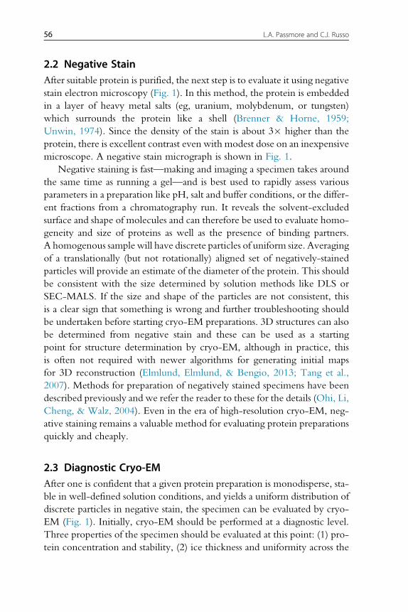
2.2 Negative StainAfter suitable protein is purified, the next step is to evaluate it using negative

stain electron microscopy (Fig. 1). In this method, the protein is embedded

in a layer of heavy metal salts (eg, uranium, molybdenum, or tungsten)

which surrounds the protein like a shell (Brenner & Horne, 1959;

Unwin, 1974). Since the density of the stain is about 3� higher than the

protein, there is excellent contrast even with modest dose on an inexpensive

microscope. A negative stain micrograph is shown in Fig. 1.

Negative staining is fast—making and imaging a specimen takes around

the same time as running a gel—and is best used to rapidly assess various

parameters in a preparation like pH, salt and buffer conditions, or the differ-

ent fractions from a chromatography run. It reveals the solvent-excluded

surface and shape of molecules and can therefore be used to evaluate homo-

geneity and size of proteins as well as the presence of binding partners.

A homogenous sample will have discrete particles of uniform size. Averaging

of a translationally (but not rotationally) aligned set of negatively-stained

particles will provide an estimate of the diameter of the protein. This should

be consistent with the size determined by solution methods like DLS or

SEC-MALS. If the size and shape of the particles are not consistent, this

is a clear sign that something is wrong and further troubleshooting should

be undertaken before starting cryo-EM preparations. 3D structures can also

be determined from negative stain and these can be used as a starting

point for structure determination by cryo-EM, although in practice, this

is often not required with newer algorithms for generating initial maps

for 3D reconstruction (Elmlund, Elmlund, & Bengio, 2013; Tang et al.,

2007). Methods for preparation of negatively stained specimens have been

described previously and we refer the reader to these for the details (Ohi, Li,

Cheng, & Walz, 2004). Even in the era of high-resolution cryo-EM, neg-

ative staining remains a valuable method for evaluating protein preparations

quickly and cheaply.

2.3 Diagnostic Cryo-EMAfter one is confident that a given protein preparation is monodisperse, sta-

ble in well-defined solution conditions, and yields a uniform distribution of

discrete particles in negative stain, the specimen can be evaluated by cryo-

EM (Fig. 1). Initially, cryo-EM should be performed at a diagnostic level.

Three properties of the specimen should be evaluated at this point: (1) pro-

tein concentration and stability, (2) ice thickness and uniformity across the


grid, and (3) phase of the ice (should be uniformly amorphous, not crystal-

line). All three should be consistent enough across the grid to yield several

squares appropriate for data collection. An example of a micrograph of a

ribosome specimen is shown in Fig. 1.

Standard substrates for cryo-EM consist of a 3-mmmetal grid which sup-

ports a perforated foil (Fig. 2) (Russo & Passmore, 2016a). Foils are patterned

with a regular array of holes (Ermantraut, Wohlfart, & Tichelaar, 1998;

Quispe et al., 2007) and can be made from various materials, the most com-

mon of which is amorphous carbon (Table 2). We recently showed that

A B C

Fig. 2 Supports for cryo-EM. Here, we show a support comprising a 3-mm metal meshgrid (A) with a perforated gold foil covering the surface of the mesh (B and C). Thin films(�2–30 Å thick) can be added on top of the perforated foil. Scale bars are (A) 0.5 mm,(B) 50 μm, and (C) 5 μm.

Table 2 Specimen Support Geometries for Particular ApplicationsMode Grid Foil Film

Negative stain 400 mesh None 50–100 A am-C

Diagnostic cryo 300 mesh 1.2/1.3 μm None/20 A am-C

Medium-resolution cryo (�3.5 A) 300 mesh 1.2/1.3 μm None/20 A am-C

High-resolution cryo (<3.5 A)

>400 kDa

300 mesh 1.2/1.3 μm None/20 A am-C

High-resolution cryo (<3.5 A)

<400 kDa

300 mesh 1.2/1.3 μm None/graphene

Very high-resolution cryo (<2.8 A) 300 mesh 0.6/1.0 μm None/graphene

Cryo-tomography: cellular

(>30 A)

200 mesh 2.0/2.0 μma None

Cryo-tomography: high-resolution

subtomogram avg. (<15 A)

300 mesh 1.2/1.3 μm None/20 A am-C

aLarger holes may be used for particularly large specimens.


making both the grid and the foil from the same material, gold, improves the

stability of the support and reduces the movement of the specimen during

imaging by more than an order of magnitude, thus improving image quality

(Russo & Passmore, 2014c).

During vitrification, proteins are preserved in a hydrated, native state in

the holes of the foil. The contrast of protein in vitreous ice is low so it is

important to ensure that the ice is only slightly thicker than the particle

diameter to maximize contrast. A water layer that is too thin will exclude

proteins and this is usually apparent from the presence of a circular region

of ice near the center of a hole where no particles are present. Given an

appropriate concentration of stable complex in the droplet, the particle dis-

tribution and ice thickness should be optimized by changing one of a few

parameters: (1) the blotting and plasma conditions, (2) adding a small amount

of detergents, and (3) adding a thin film of amorphous carbon or graphene to

the surface of the foil to induce adsorption of particles across the holes. Cur-

rently, this remains a trial and error process and so must be done in a way that

minimizes uncontrolled changes.

Proteins often denature when they come into contact with surfaces

(Seigel et al., 1997), and several are present during the vitrification process.

These include the hydrophobic air–water interface, amorphous carbon sup-

port layers, copper, gold, and other metals used to create grids, and even the

cellulose paper used to blot away the excess liquid. Of these, the air–waterinterface is likely the most problematic as the requirement for a thin layer of

water ice means the particles must be brought in close proximity to one just

before freezing. Its hydrophobic nature means it is likely to induce the

adsorption, and possible denaturation, of many proteins and complexes

(Seigel et al., 1997; Vogler, 2012).

For a given concentration of protein, one can calculate the number of

particles that should be found in the thin layer of vitreous ice. For example,

for a 1-MDa protein in 800 A thick vitreous ice, a solution of 2 mg/ml

should give approximately 100 particles/μm2. A 250-kDa protein at the

same concentration should give approximately 400 particles/μm2. Often,

the protein concentration in solution does not match the protein concen-

tration on the support: protein density can be higher than expected if the

particles tend to adsorb to the surface, or lower if they tend to repel

the surface (or are attracted to the support or other surfaces like the blotting

paper instead). Changing the buffer conditions (eg, changing pH or

salt concentration, adding detergents, lipids, or other chemical modifying

agents like cross-linkers) may change the interaction of proteins with


surfaces (Cheung et al., 2013; Dubochet et al., 1985; Glaeser et al., 2016).

A support that is too hydrophobic, for example because of insufficient

plasma treatment or contamination with hydrocarbons, can strongly adsorb

proteins to itself, making the concentration of particles in the holes much less

than was in the applied droplet. This is a clear indication that there is a prob-

lem with the specimen. The opposite situation can also occur. That is, the

particles can adhere to the air–water interface, artificially concentrating themprior to the removal of most of the water and the creation of the thin layer.

This leads to a particle concentration in the holes that is much higher than it

was in the droplet; also a clear indication that there is a problem with the

specimen. Often, the particles adhered to the interface will have low contrast

and will be partially or fully denatured. In addition, the particles will appear

larger in size than expected as they unfold to varying degrees on the surface

(Seigel et al., 1997). This should be resolved beforemoving on to collect large

datasets in cryo.

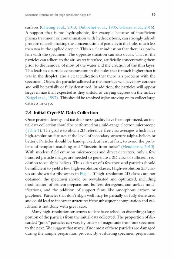
2.4 Initial Cryo-EM Data CollectionOnce protein density and ice thickness/quality have been optimized, an ini-

tial data collection should be performed on a mid-range electron microscope

(Table 1). The goal is to obtain 2D reference-free class averages which have

high-resolution features at the level of secondary structure (alpha-helices or

better). Particles should be hand-picked, at least at first, to avoid the prob-

lems of template matching and “Einstein from noise” (Henderson, 2013).

With modern field emission microscopes and direct detectors, only a few

hundred particle images are needed to generate a 2D class of sufficient res-

olution to see alpha helices. Thus a dataset of a few thousand particles should

be sufficient to yield a few high-resolution classes. High-resolution 2D clas-

ses are shown for ribosomes in Fig. 1. If high-resolution 2D classes are not

obtained, the specimen should be reevaluated and optimized, including

modification of protein preparations, buffers, detergents, and surface mod-

ifications, and the addition of support films like amorphous carbon or

graphene. Particles that don’t align well may be partially or fully denatured

and could lead to incorrect structures if the subsequent computation and val-

idation is not done with great care.

Many high-resolution structures to date have relied on discarding a large

portion of the particles from the initial data collected. The proportion of dis-

carded “junk” particles can vary by orders of magnitude from one specimen

to the next. We suggest that many, if not most of these particles are damaged

during the sample preparation process. By evaluating specimen preparation


using the above criteria, one can optimize the specimen and improve particle

yield. This is generally preferable to collecting large datasets and discarding

most particles to reach a desired resolution. Improving particle yield will

make the entire process more efficient and more likely to succeed.

Once a preliminary dataset is collected that generates suitable 2D classes,

a larger dataset with a few hundredmicrographs and several tens of thousands

of particles is collected on a mid-range or high-end microscope, from which

an initial 3D map can be calculated. Several important factors can then be

evaluated. First, do the 2D classes show several distinct views of the particle,

with self-consistent dimensions, each with secondary structural features?

Second, is the orientation distribution sufficient to allow calculation of a

3D structure with isotropic resolution? Fig. 1 shows an equal area projection

map of the orientation angles of ribosomes relative to an amorphous carbon

substrate. Although these ribosomes exhibit preferred orientations, they

cover Fourier space sufficiently for a high-resolution structure. If the orien-

tation distribution is not suitable, one can alter buffers, add detergents,

change plasma conditions, or use an alternative surface, eg, graphene or

amorphous carbon to improve the distribution and promote additional

views of the complex. Cross-linking can also alter particle orientations since

modification of charged surface amino acids (often lysines) changes the sur-

face properties of molecules and their interaction with the supporting sur-

faces and the air–water interface (Bernecky, Herzog, Baumeister, Plitzko, &

Cramer, 2016). Collecting small datasets will be sufficient to determine if

any changes in preparation conditions were effective at improving the ori-

entation distribution.

2.5 High-Resolution Data CollectionIf the resolution of the initial 3D reconstruction reaches a reasonable reso-

lution for the number of particles and image acquisition settings, a larger data

collection on a high-end electron microscope should be performed with the

aim of obtaining a high-resolution structure (Fig. 1). What constitutes a

“reasonable resolution” will be arbitrary and should ultimately depend on

the resolution of the biological question and the state of the technology,

but as a guideline, we suggest that currently, subnanometer resolution

should be routinely possible from 10 to 50 thousand asymmetric particle

images. With this in mind, a large dataset (500–1000 micrographs, �24 h

of microscope time) should be collected with the best available microscope:

currently this is a 300 keV instrument with one of several commercially

available direct electron detectors (Tables 1 and 3). The data collection strat-

egy will depend on the size of the particle, the resolution desired, and the


Table 3 Current Electron Detectors for CryomicroscopyDetector Type Current Examples Pixel Pitch Num. Pixels Frame Rate (Hz) Recommended Flux (Optimum [Range] e2/px/s)

Phosphor–CCD Gatan Orius 830 7.4 2048 � 2048 1 –Gatan US1000 14 2048 � 2048 1.5/15 –

Phosphor–CMOS Tietz TemCam 15.6 4096 � 4096 1 –Gatan OneView 15 4096 � 4096 25 –FEI Ceta 14 4096 � 4096 32 –

Direct integrating Direct El. DE16a 6.5 4096 � 4096 60 � 240

Direct El. DE20a 6.4 5120 � 3840 32 � 100

FEI Falcon 2a 14 4096 � 4096 18 50 [10–60] (300 keV)40 [8–48] (200 keV)b

FEI Falcon 3a 14 4096 � 4096 32 100 [20–120] (300 keV)

Direct counting Gatan K2 5 3838 � 3710 400 5 [2–8] (300 keV)

aThese detectors can also be operated in electron counting mode but current frame rates make this impractical for normal data collection.

bThe flux, f0 at one energy can be scaled with reasonable accuracy to other energies relevant to transmission electron microscopy using the equation f1 ¼ f0β21β20, where β is

the ratio of the electron velocity to the speed of light.

particular microscopes available to the microscopist. Our current recom-

mendations for data collection on various specimen types are discussed in

Section 8.

All biomolecular complexes exist in multiple conformational states, and

for each to be resolved, even more high quality data are required. Many

computational algorithms are available to help extract this information

from a dataset and we refer the reader to chapters “Processing of Structurally

Heterogeneous Cryo-EM Data in RELION” by Scheres, “FREALIGN:

An Exploratory Tool for Single-Particle Cryo-EM” by Grigorieff, and

“Single Particle Refinement and Variability Analysis in EMAN2.1” by

Ludtke for more details. In some cases, ligands (eg, small molecules, binding

partners, and nucleotides) can be added to stabilize particular conformations,

or to interrogate a particular biological question related to how a ligand

affects the conformational state of the complex. These usually require the

collection of additional large datasets to achieve high-resolution after small

datasets have been collected to confirm the change in conformation or

presence of the ligand of interest.

Finally, but perhaps most importantly, all high-resolution datasets

should be collected with validation in mind (see chapter “Testing the Valid-

ity of Single Particle Maps at Low and High Resolution” by Rosenthal). In

particular, we recommend collecting a small set of tilt-pairs (�1–2% of the

number of micrographs) with every dataset intended for determination of a

previously unknown structure. They can be subsequently used to validate

the reconstructed density map (Baker, Watt, Runswick, Walker, &

Rubinstein, 2012; Henderson et al., 2011; Rosenthal & Henderson,

2003; Wasilewski & Rosenthal, 2014), measure the angular accuracy of

the projection assignments (Russo & Passmore, 2014b), and determine

the absolute hand of the structure (Rosenthal & Henderson, 2003).

By using the systematic approach described earlier, the microscopist will

have the best chance of efficiently going from a protein in solution to a high-

resolution structure. In the following section, we describe many of the prac-

tical methods and details of the processes that are important to successful

specimen preparation. This includes a series of protocols that are intended

to help guide the reader in the current state-of-the-art, and hone the tech-

niques of new microscopists.

3. SUPPORT CHOICE, HANDLING, AND STORAGE

A fundamental but often overlooked factor in preparing high quality

specimens for cryo-EM is correct handling and storage of the supports. They


are delicate and can easily be damaged or contaminated, compromising later

steps in the process and reducing reproducibility. Before starting, it is useful

to check supports using an optical microscope and discard any with defects,

large areas of broken squares or contamination. The time spent checking

supports in a light microscope is trivial compared to subsequent time spent

preparing and imaging the specimen. The supports should start and remain as

flat as possible to prevent damage to the foil. Importantly, supports should

always be handled with sharp tweezers and picked up by the rim only

(Fig. 3). We like to use tweezers with a normally closed configuration

(eg, Dumont type N5) as this applies a well-defined and reproducible force

A B

C D

Fig. 3 Tweezer damage to specimen supports. Bent tweezers (A) or improper use(B) results in damage to the specimen support. For best results, sharp, straight tweezers(C) should be used and supports should be picked up by the rim only (D). For panelsA and C, the scale bars are 1 mm. For panels B and D, the scale bars are 100 μm.


to the grid during handling. Static discharge can also damage supports but

this can be eliminated by wearing a wrist grounding strap whenever han-

dling supports (Fig. 4). We do not recommend wearing a glove on the hand

that holds the tweezers as this induces static buildup on the tweezer/support

and reduces dexterity. After cleaning or modification, supports should be

stored in glass, not plastic, petri dishes, and in clean, oil-free dry boxes to

keep them clean and dust free.

To prevent carry-over of specimens and to remove contamination, grid

handling implements, glass slides, and glass dishes should be thoroughly

cleaned on a regular basis. Glass can be cleaned by sonicating in a high-purity

detergent mixture (eg, 2% Micro-90) and rinsing with ultra-pure, 18 MΩdeionized water. Tweezers can be cleaned after routine use by sonication

in alcohol (ethanol or isopropanol) or with more aggressive solvents like

chloroform and acetone if they have been contaminated with plastic or

oil residues. Note that tweezers used for grid plunging should be

decontaminated with ethanol sonication after each distinct specimen, as

cross-contamination from one grid to the next via the tweezers is common.

Supports with irregular arrangements (lacey or holey carbon) or regular

arrays of holes are available but the latter, eg, Quantifoil, UltrAuFoil, C-flat,

are more reproducible and simplify data collection methods. A detailed dis-

cussion of support types can be found in Russo and Passmore (2016a). Here,

we provide recommendations for support geometries for various applica-

tions (Table 2).

As to the choice of material, we recommend amorphous carbon (am-C)

on copper for negative stain, as they are commonly available and inexpen-

sive, and all-gold supports for cryo-EM as they reduce the movement

BA

Glass dishPlastic dish

Glovedhand

No glove

Wrist grounding strap

Fig. 4 Storing grids to avoid contamination and static charge. Panel A shows bad practicein grid handling: The use of gloves and plastic storage dishes results in the accumulationof static charge. In the image, a charged grid is standing on end. Panel B shows rec-ommended handling procedures including glass containers, no glove on the hand hold-ing the tweezers and a wrist grounding strap to prevent accumulation of charge.


of specimens and improve image quality (Russo & Passmore, 2014c).

All-gold supports can be made using the protocols described in Russo

and Passmore (2016b) or are commercially available from Quantifoil

(UltrAuFoil®).

4. CONTAMINATION AND CLEANING

Even under optimal storage conditions, supports may need to be

cleaned prior to use. Contamination can arise from particulate matter

including flakes of evaporated carbon, residual particles from manufacturing

processes or accumulated dust from storage. If these are not removed, they

will be resuspended upon application of the aqueous protein solution and

may be visible in the vitreous ice, which can interfere with subsequent data

processing and analysis. In addition, contamination can arise from organic

residue deposited on the surface during handling or storage, and from resid-

ual photoresist or other plastics and solvents used during the manufacturing

processes. Such surface residues can affect wetting and other material prop-

erties of the support and reduce reproducibility.

Here, we provide a method to clean supports by water and solvent

washes prior to use (Protocol 1). Ultra-high purity (CMOS grade) solvents

are required for cleaning without contamination. We do not recommend

cleaning supports by heating as this can compromise the structural integrity

of the support.

Warning: The protocols described here involve using high voltage, high

temperatures, liquid nitrogen, hazardous and flammable chemicals/gases,

and equipment under vacuum. They are for use by experienced scientists

who know how to handle such equipment and have done all appropriate

local safety training and risk assessments, etc. Wear safety glasses, appropriate

protective equipment, and use at your own risk.

Protocol 1. (Support cleaning)

1. Fill a clean, glass crystallization dish (Pyrex, diameter 90 mm, height

50 mm) with deionized water (18 MΩ, filtered, UV treated). Overfill

it to break the meniscus at the surface and remove any contaminating

surface layers on the water (Fig. 5C).

2. Using small, clean glass test tubes, prepare three solvent washes (Fig. 5A):

one with 1 ml chloroform (Sigma 650498), one with 1 ml acetone

(Sigma 40289), and one with 1 ml isopropanol (Sigma 40301). Use glass

pasteur pipettes as the solvents can dissolve and redeposit residue from

most plastics.


3. Pick up a single support using clean tweezers (Dumont N5 or 5) and

dunk it into the water at one side of the dish. As the grid enters the water,

loose contamination can float off onto the surface of the water. Pulling

the grid out in the same place will result in the contamination being

redeposited on the grid surface. Move the grid through the water to

remove it from the opposite side of the dish. (Ensure it is moved through

the water with the thin edge leading to prevent damage to the perforated

foil.) Touch edge of grid briefly to filter paper (Whatman No. 1) to

remove excess water, but take care not to bend the grid. If not using anti-

capillary tweezers, blot between the tines.

4. Dunk grid sequentially in chloroform, acetone, and isopropanol (pre-

pared above) for 10–20 s each. It is particularly important that the final

rinse step is in the cleanest possible solvent as any residue from it will be

deposited on the grid surface. If not using anticapillary tweezers, blot

between the tines after each rinse to remove excess.

5. Touch edge of grid briefly to filter paper to remove excess isopropanol.

B

Grid

Tweezers

Contamination

Liquid solvent

C

A

Fig. 5 Removing surface contamination from specimen supports. Supports can bewashed sequentially (A) in chloroform, acetone, and isopropanol. Care must be takento avoid deposition of contamination from the surface of water (or solvents) ontothe support. A schematic is shown in panel B. Overfilling of containers can reduce sur-face contamination, shown in panel C. Scale bars are 20 mm.


6. Place grid on filter paper (Whatman No. 1, 70 mm rounds) in clean glass

petri dish (Schott, 70 mm), foil side up, to dry. Cover with glass lid to

minimize dust accumulation.

7. Store in the covered glass petri dish after drying but use soon after

cleaning.

5. CONTINUOUS FILMS OF AMORPHOUS CARBONAND GRAPHENE

A continuous film of amorphous carbon or graphene provides an

alternative surface for proteins to interact with. In some cases, this improves

protein distribution or orientation within the vitreous ice. In addition, lower

protein concentrations can sometimes be used because the particles adsorb to

the surface before blotting away the excess liquid. Here, we provide a pro-

tocol for producing thin (20–50 A) films of amorphous carbon for use as a

surface for particle adsorption. The same protocol can be used for thicker

films (50–100 A) of carbon appropriate for transfer to bare grids (no perfo-

rated foil) for negative stain.

Protocol 2. (Amorphous carbon deposition)

This protocol is for depositing carbon onto a sheet of mica using an Edwards

306 Turbo coating system equipped with an Inficon crystal thickness mon-

itor with water cooling, but can be adapted to other deposition systems.

1. Vent the chamber and remove the implosion guard and bell jar.

2. Put on clean gloves and handle everything inside the chamber with

gloves.

3. Remove the carbon source apparatus, remove the shield and mount a

new sharpened carbon rod (high purity graphite < 5 ppm impurity),

under tension, in the chuck.

4. Use compressed nitrogen to blow out any bits of carbon or flakes as

these can cause a short between the electrodes.

5. Replace the source in the chamber, with the rod positioned 125 mm

from the stage. Finger tighten the nuts (no wrench).

6. Mica is a multilayered mineral crystal which is extremely flat (less than

1 nmRMS per mm2) and easy to obtain in large sheets, and so is used as

a template surface for carbon deposition. Cleave a piece of mica

(eg, Agar G250-1) in half with a razor blade and position the two sheets,

cleaved surface up, on the specimen stage directly beneath the source

on top of a fresh piece of filter paper (Whatman no. 1). Mica should be

cleaved immediately before coating as the freshly cleaved surface is


clean and hydrophilic, but it becomes contaminated (and thus hydro-

phobic) with time spent in air.

7. A clean penny or other small piece of metal can be used to hold the mica

sheets and filter paper in place during evacuation.

8. Check the position of the shutter in the open and closed state: closed it

should cover the solid angle from the source to the mica and the crystal

thickness monitor. In the open state, the paths to both the mica and the

crystal should be unobstructed and equal in length. Leave in the closed

position.

9. Check the bell jar gasket and base plate for any dust, dirt, or flakes of

carbon or metal. Clean with lint free paper and methanol if necessary.

10. Replace the bell jar and implosion guard.

11. Fill the liquid nitrogen cold trap.

12. Evacuate the chamber by pressing cycle on the panel.

13. When the gate valve opens, the pressure should drop rapidly into the

10�5 Torr range. Begin heating the source apparatus by turning on the

low tension power supply (LT) and slowly increasing the current to

about 1.0 Amp.

14. Wait 10 min and increase the current to 1.2 Amps.

15. Wait 5 min and increase to 1.4 Amps.

16. Leave at 1.4 amps for 20 min. Then shut off. Top up the liquid

nitrogen.

17. Turn on the cooling water to the crystal thickness monitor and check

the correct program for carbon is selected. Zero the thickness.

18. Vacuum should now drop to the 10�7 Torr range in about an hour.

19. Once vacuum is < 5 � 10�7 Torr, slowly ramp up the current again

to 1.6–1.7 Amps over about 5 min, being careful not to let it spark.

The pressure should not rise above < 5 � 10�6 Torr as the source is

heated.

20. Once the carbon begins to deposit, the current will start to fluctuate.

Open the shutter and deposit for 10–20 s, then close the shutter and

turn the current back down slightly.

21. The crystal will initially go negative as it heats up but after closing the

shutter, it will return to a positive value which is the accumulated thick-

ness. This can be repeated until the desired thickness is reached.

22. When finished evaporating, close the shutter and turn off the power to

the source.

23. Let the chamber cool for at least 30 min before venting.


24. Vent with dry nitrogen, remove your coated mica and store in a glass

Petri dish.

25. Replace the bell jar and implosion guard, press cycle, wait for the vac-

uum to reach 200 mTorr and then press seal.

Notes: The crystal thickness monitor should be calibrated according to the

manufacturer using an independent thickness measurement method. We

have used atomic force microscopy in the past for this purpose (Russo &

Passmore, 2014a). Carbon density can vary depending on the quality of your

source material but should be approximately 2.2 g/cm3. From start to finish,

the process should take less than 4 h. Unless using a fully dry (no oil)

pumping system, overnight pumps are not recommended as oil will back-

stream into the chamber when the liquid nitrogen trap is not cold and this

will contaminate the chamber and mica with oil.

We previously provided a detailed protocol for transferring amorphous

carbon onto supports (Russo & Passmore, 2016b) and we have had good

results using this with Quantifoil and all-gold supports. This is reproduced

here in Protocol 3.

Protocol 3. (Amorphous carbon transfer onto supports)

1. Wear wrist grounding strap to prevent static damage to supports during

handling. Don’t wear a glove in the hand that holds the tweezers, or

ground the tweezers directly.

2. Inspect supports in dissecting microscope and discard any with defects.

All grids should be flat, continuous, and without dust or lint.

3. If there is evidence of residual plastic from lithographic processing, they

can be cleaned using Protocol 1.

4. Using gloves to prevent fingerprints and contamination, place filter

paper (Whatman No. 1, diameter 70 mm) on a stainless steel mesh cir-

cle (diameter 65 mm, made with 0.7 mmwire with 3 mmmesh) inside

a stainless steel ring (polished and beveled edges, 2 mm thick, height

10 mm, diameter 50 mm) in a glass crystallization dish (Pyrex, diameter

90 mm, height 50 mm) (Fig. 6) (Russo & Passmore, 2016b).

5. Fill dish with deionized water (18 MΩ, filtered, UV treated). Overfill it

to break the meniscus at the surface and remove any contaminating sur-

face layers on the water (Fig. 5C). Pour off excess water so the level is

just below the rim of the glass dish.

6. Using tweezers (Dumont N5 or 5, cleaned by solvent rinse), carefully

place grids, foil side up, onto the center of the filter paper. The grids

should enter the water slowly and perpendicular to the surface.


7. Setup a siphon: attach tubing (length 0.6 m, outer diameter 3.2 mm,

inner diameter 1.6 mm) to dish with normally closed forceps or a spring

clip. Start flow of syphon with syringe and clamp off flowwhile floating

the carbon (next step).

8. Float carbon off mica by slowly lowering a ’ 2.5 � 2.5 cm sheet of

amorphous carbon coated mica (carbon-side up) into the water at a

20–30° angle. A light can be placed to shine off the surface of the water

at a glancing angle, allowing you to see the carbon better.

9. Use the siphon to slowly lower the water level.

10. Monitor the position of the carbon with respect to the grids and ensure

it stays centered by gently nudging with clean tweezers.

11. Once the carbon has been deposited on the grids and the water level is

below the filter paper, carefully lift off the stainless steel ring. Remove

the filter paper and mesh together. Place on a dry sheet of filter paper

and cover with a clean glass petri dish or beaker, tilted slightly to leave

room for evaporation. Allow several hours to dry.

12. When dry, store in a clean glass petri dish until ready to use.

Graphene is superior to amorphous carbon due to its defined structure and

conductive properties (Geim, 2009; Pantelic, Meyer, Kaiser, Baumeister, &

Plitzko, 2010; Pantelic et al., 2011; Russo & Passmore, 2014a). In addition,

Siphon

Thinamorphous carbon

Stainlesssteel ring

Glasscrystallization

dish

Supports Stainlesssteel mesh

Filterpaper

Flow

A B

Fig. 6 Apparatus for depositing thin films of amorphous carbon on supports. PanelA shows a cross-sectional diagram of the float chamber. As the water level is lowered,the thin film of amorphous carbon is deposited onto the supports. The stainless steelring makes a positive meniscus to help lower the carbon film down in the center ofthe ring. Panel B shows a photo of the apparatus in use. This figure is reproduced fromRusso, C. J., & Passmore, L. A. (2016b). Ultrastable gold substrates: Properties of a support forhigh-resolution electron cryomicroscopy of biological specimens. Journal of StructuralBiology, 193 (1), 33-44. doi: 10.1016/j.jsb.2015.11.006. Drawings are available from theauthors.


it is effectively invisible at the resolutions of interest for cryo-EM, whereas

amorphous carbon adds additional background noise that is especially det-

rimental for smaller proteins. Here, we provide procedures for transferring

graphene onto Quantifoil supports (Fig. 7, Protocol 4) (Regan et al., 2010;

Russo & Golovchenko, 2012). Ultra-high purity (CMOS grade) solvents

and acids are required for reliable transfers without contamination and a

wrist grounding strap should be worn at all times to prevent static damage

to supports during handling since graphene films are particularly sensitive to

A

Graphene

Copper

Gold grid

Perforated carbon

Adhere carbon membrane tographene by solvent wetting

Ferric chloride

Etch away the copper substrateby floating it in FeCl3

Final suspended grapheneelectron microscope support

B D F

C E G

Fig. 7 Graphene transfer onto supports with carbon foils. The process is diagrammed inpanel A. Panels B and C show copper heated to 150°C for 10 min in air, where B is fullycovered in graphene so does not oxidize while C has no graphene and turns color due tooxidization, scale bars are 3 mm. This simple test is used to map the location of thegraphene on the foil. Panels D and E show the grid–graphene–copper sandwich, scalebars are 1 mm and 10 μm, respectively. Panel F is the sandwich floating in the etchant,where the partially etched grains of copper are visible (scale 1 mm). Panel G is an elec-tron diffraction pattern of suspended graphene with ice, where the arrow points to the2.1 Å reflection from the graphene lattice.


static discharge. All glassware should be cleaned prior to use. A new transfer

protocol for all-gold supports is currently under development, and we

expect that graphene on all-gold supports will become commercially

available.

Protocol 4. (Graphene transfer onto supports)

1. Inspect freshly cleaned supports (Quantifoil Au 300 1.2/1.3, see

Protocol 1) in dissecting microscope and discard any with defects.

2. Graphene is grown on thin sheets of copper using chemical vapor

deposition (CVD) and can be purchased from commercial vendors

(Graphene Supermarket, Structure Probe Inc., etc.). Punch out

3.2 mm disks from copper/graphene source material where the copper

has been checked for the presence of graphene (Fig. 7B, C). We use a

custom-mademechanical punch but these are also available from Struc-

ture Probe, Inc.

3. Place a support, foil side down, on each disk.

4. Press together between two clean glass slides and then remove the top

glass slide.

5. Using a clean pipet, add 7 μl of isopropanol (Sigma 40301) to the top of

the grid–graphene–copper sandwich and let dry.

6. Inspect in high-resolution optical microscope to check for adherence of

the carbon foil to the copper. The foil changes color when well adhered

to the copper surface, (Fig. 7E) and only well-adhered regions will

transfer successfully.

7. Layout and label seven borosilicate glass crystallization dishes (70 mm

diameter) in fume hood.

8. Fill first crystallization dish 2/3 full with copper etchant containing

buffered FeCl3 (Sigma 667528).

9. Gently place the support disk sandwiches on the surface of FeCl3 by

sliding off glass slide. Cover with borosilicate glass Petri dish covers

(80 mm) to keep out dust during the etch.

10. Etch for 20 min in FeCl3 (for 25 μm thick copper).

11. Fill three dishes 2/3 with 20% HCl (Sigma 40233), 20% HCl and

2% HCl.

12. Transfer grids to each using a flamed platinum loop (homemade or

EMS 70944). Leave floating for 10 min at each step.

13. Overfill three more dishes with cleanest possible water.

14. Transfer to each using platinum loop, and rinse for 3–5 min each.

15. Use loop to transfer and flip, graphene side up, onto filter paper

(Whatman No. 1, 70 mm rounds). Let dry in clean borosilicate glass

Petri dish (70 mm).


16. Dispose of acids in appropriate hazardous waste streams.

17. Store long term in glass in a dry environs free of any type of oils or

hydrocarbons. Do not store in any type of plastic container.

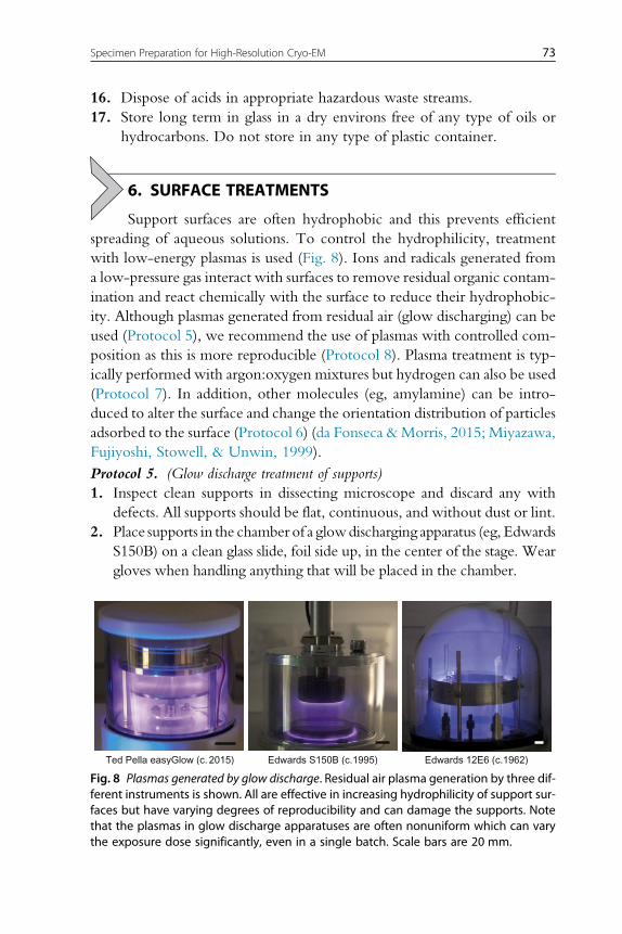
6. SURFACE TREATMENTS

Support surfaces are often hydrophobic and this prevents efficient

spreading of aqueous solutions. To control the hydrophilicity, treatment

with low-energy plasmas is used (Fig. 8). Ions and radicals generated from

a low-pressure gas interact with surfaces to remove residual organic contam-

ination and react chemically with the surface to reduce their hydrophobic-

ity. Although plasmas generated from residual air (glow discharging) can be

used (Protocol 5), we recommend the use of plasmas with controlled com-

position as this is more reproducible (Protocol 8). Plasma treatment is typ-

ically performed with argon:oxygen mixtures but hydrogen can also be used

(Protocol 7). In addition, other molecules (eg, amylamine) can be intro-

duced to alter the surface and change the orientation distribution of particles

adsorbed to the surface (Protocol 6) (da Fonseca &Morris, 2015; Miyazawa,

Fujiyoshi, Stowell, & Unwin, 1999).

Protocol 5. (Glow discharge treatment of supports)

1. Inspect clean supports in dissecting microscope and discard any with

defects. All supports should be flat, continuous, and without dust or lint.

2. Place supports in the chamber of a glowdischarging apparatus (eg, Edwards

S150B) on a clean glass slide, foil side up, in the center of the stage. Wear

gloves when handling anything that will be placed in the chamber.

Ted Pella easyGlow (c. 2015) Edwards S150B (c.1995) Edwards 12E6 (c.1962)

Fig. 8 Plasmas generated by glow discharge. Residual air plasma generation by three dif-ferent instruments is shown. All are effective in increasing hydrophilicity of support sur-faces but have varying degrees of reproducibility and can damage the supports. Notethat the plasmas in glow discharge apparatuses are often nonuniform which can varythe exposure dose significantly, even in a single batch. Scale bars are 20 mm.


3. Pump the chamber to 200 mTorr.

4. Turn on the HT to 7 kV, current should be 28–30 mA.

5. Expose the supports for 30 s.

6. Turn off the HT and slowly vent the chamber.

7. Store the treated supports in a clean glass petri dish and use as soon as

possible (within 1 h).

Protocol 6. (Amylamine plasma treatment of supports)


All supports should be flat, continuous, and without dust or lint.

2. Place supports in the chamber on a clean glass slide, foil side up, in the

center of the electrode ring (Fig. 8).

3. A small glass vial containing 0.5 ml of amylamine is placed in the cham-

ber at the edge of the stage.

4. Cover with the bell jar and pump the chamber to below 400 mTorr.

5. Turn on theHT and adjust the power to form a uniform plasma (� 90 V,

1.5 A for our system).

6. Expose the supports for 30–60 s.7. Turn off the HT and slowly vent the chamber. Discard the vial in an

appropriate waste stream.

8. Store the treated supports in a clean glass petri dish and use within 1 h.

Protocol 7. (Argon oxygen plasma treatment)


All supports should be flat, continuous, and without dust or lint.

2. We use a Fischione 1070 plasma chamber with a custom suspension

holder that holds up to 10 supports (Fig. 9). In this configuration, the

grids are 15 � 1 cm from the radio frequency coils. It is desirable to

always position the grids in the same location relative to the plasma to

improve the reproducibility of the exposures from batch to batch. Alter-

natively, the specimens can be placed directly in the chamber on a clean

glass slide, foil side up, on the shelf in the chamber. Plasmas that are not

well shielded or not sufficiently low in energy may damage gold supports

by sputtering; this should be avoided. Load up to 20 supports into the

plasma chamber. Everything that goes inside the vacuum chamber should

be handled with gloves to prevent contamination and fingerprints.

3. Evacuate chamber to ≪ 10�4 Torr.

4. Admit high purity argon and oxygen (BOC 99.9999%) in a ratio of 9:1

to a pressure of 21 mTorr (31.0 SCCM gas flow).

5. Apply radio frequency plasma with 38 W of forward power and � 2 W

of reverse power (�70% setting on a Fischione 1070) for 10–60 s


(20–30 s works well for most supports). The time can be optimized for

suitable hydrophilicity (spreading of aqueous solution and ice thickness).

For amorphous carbon-containing supports, calibrate the carbonetch rate

empirically by performing several plasma treatments of increasing dose

and determining when a carbon layer of known thickness is fully etched.

6. For very thin films of continuous carbon, use a ratio of 19:1 argon:

oxygen and 35 W forward power for 5–15 s.7. Vent plasma chamber, remove supports and use within 1 h.

Using a low-energy hydrogen plasma, one can remove contamination and

control protein adsorption onto graphene (Russo & Passmore, 2014a).

Here, we provide the procedure for hydrogen plasma treatment using a

Fischione 1070 with a Dominik Hunter model 20H-MD hydrogen gener-

ator, attached to one of the input ports of the plasma generator. Hydrogen

plasma treatment is stable but should be performed immediately prior to use

to minimize accumulation of contamination after modifying the surface.

Gatan Solarus

A

B

C

D

Fischione Model 1070

Gas Plasma

RF coil

e–

R+R–

R•e–

Custom holder for Fischione

One side exposure

Two side exposure

Lid

Grids

Lid

Fig. 9 Generation of defined plasmas for surface modification. (A and B) The FischioneModel 1070 and Gatan Solarus generate plasmas with defined compositions.(C) Photo (top) and diagram (bottom) of a custom specimen holder made at MRCLMB. Two different holder designs are shown—one is used for exposure of one sideof a support and the other is used for exposure of both sides. The lid is used to preventthe supports from moving during the process. (D) Diagram of plasma generation.


Protocol 8. (Hydrogen plasma treatment of graphene supports)

1. Use only ultra-high purity hydrogen (>99.999% pure), all stainless

steel tubing and fittings (no plastic), and ultra-high purity grade

regulators.

2. The distance of the coils to the sample is important since it affects the

energy of the hydrogen species. A plasma where atoms and ions strike

the surface and recoil, delivering an energy greater than �21 eV to

the carbon atoms, might cause significant damage to the lattice rather

than chemically modifying it. The energy of the plasma vs distance

can be measured with a Langmuir probe to ensure that the energy is

below the �21 eV sputter threshold at the sample. Alternatively, one

can test whether the energy is too high by imaging a graphene-covered

support before and after increasing doses of hydrogen plasma to deter-

mine whether it remains intact.

3. Prior to hydrogen plasma treatment, the plasma chamber should

be pretreated. Insert the holder and evacuate the plasma chamber to

≪ 10�4 Torr.

4. Burn the empty holder for 10 min in 100% pure hydrogen (70% power

which is 35 watts forward,≪ 2 watts reverse power, 20 SCCM gas flow,

pure hydrogen). Vent only just prior to loading.

5. Mount graphene supports in holder, load, and evacuate the plasma

chamber to ≪ 10�4 Torr.

6. Treat with 5–40 s (typically 20 s) hydrogen plasma using the same

settings.

7. Carefully remove the supports and use immediately.

7. VITRIFICATION

Vitrification was first developed by Jacques Dubochet and colleagues

in the 1980s (Adrian et al., 1984; Dubochet et al., 1988). To successfully

make vitreous ice, a thin layer of protein solution must be cooled quickly

so that it remains in an amorphous, noncrystalline state. This is usually per-

formed in an apparatus which plunges the specimen into a liquid cryogen

(usually ethane or propane) such that it is cooled about 200 K in < 10�4 s.

For water to vitrify, the temperature has to drop faster than 105–106 K/s(Dubochet et al., 1988). Water is a poor thermal conductor so the sample

must be less than 3 μm thick. Several designs for manual and semiautomated

plungers are available for vitrification of biological specimens, including


commercial models from FEI, Leica, EMS, and Gatan. These provide con-

trolled temperature and humidity throughout the process, preventing evap-

oration, and making specimen preparation more reproducible.We note that

after blotting, even a small amount of evaporation, equivalent to a few hun-

dred monolayers of water, can concentrate the salt and change the pH of a

suspended thin layer by a factor of two or more. For example, at 4°C and

90% relative humidity, the evaporation velocity is of order 100 A/s so in

the 2 s between the blot and the freeze, a 400 A film can be concentrated

by a factor of two, causing significant osmotic and conformational changes

in the specimen. Sowe also recommend that the relative humidity surround-

ing the specimen support always be kept at 100% to prevent deleterious

changes in the concentration of solutes just prior to freezing. This is easiest

to achieve at 4°C, because much less water vapor per unit volume is required

to bring the dewpoint to the air temperature, thus preventing evaporation. It

is also important to work quickly once sample is applied to the support to

minimize the interaction time of proteins with the often destructive, air–water interface.

A detailed discussion of vitrification procedures can be found in Dobro,

Melanson, Jensen, and McDowall (2010) and we recommend consulting

this review for further information. We include here the standard settings

we use as a starting point and other recent work can be consulted for further

advice (Thompson, Walker, Siebert, Muench, & Ranson, 2016), including

more advanced techniques like time-resolved cryo-EM (Chen et al., 2015).

The following procedure using a Vitrobot (FEI) works well for all-gold and

standard Quantifoil supports:

Protocol 9. (Standard vitrification procedure)

1. Fill cryoplunger reservoir with fresh deionized water (18 MΩ) andequilibrate to 4°C and 100% relative humidity.

2. Ensure Vitrobot tweezers (FEI, Ted Pella 47000-500) are sharp by

examining under an optical microscope. Check that they are not bent

and symmetrically aligned in the following way: place on a flat surface

and measure the tip to surface distance. Do this for all four sides; it

should be the same (within 0.5 mm) for opposing sides.

3. Clean tweezers and blotting pads with ethanol; and clean the ethane

cup, grid box holder, and foam dewar with a high purity detergent

(2% Micro-90 in Milli-Q water); rinse with Milli-Q deionized water

and dry completely.

4. Place new filter paper rounds (Whatman 595) on blotting pads.


5. After cryo-plunger is equilibrated (for at least 20 min to saturate the

water in the filter paper) and just prior to specimen vitrification, cool

down the plunging dewar with liquid nitrogen then fill the central cup

with ethane (Dobro et al., 2010). Warning Liquid ethane can cause

severe burns and blindness if splashed in the eye. Always wear safety

glasses when handling.

6. Check that the temperature of the ethane is just above the melting

point, 90 K.

7. Make supports hydrophilic by plasma treatment, as described earlier.We

emphasize that only clean, flat, intact supports should be used (see earlier).

Bent supports will be further damaged upon cryo-plunging (Fig. 10).

8. Mount a support in clean cryo-plunger tweezers. Use the foot pedal

trigger on the Vitrobot to reduce the delay time between steps in

the process.

DC

A

Cryogen Cryogen

B

Fig. 10 Vitrification and mounting of grids. (A) Supports that are bent will be damagedupon cryo plunging, resulting in broken foils. An example of a broken gold foil is shownin panel B (scale bar 2 μm). Supports also need to be mounted correctly in microscopecartridges. Panel C shows a support that is incorrectly mounted, and so damaged, in aKrios cartridge. The support in panel D is correctly mounted. Scale bars in panels C andD are 500 μm.


9. Apply 3 μl protein solution (usually 10–5000 nM) to the foil side.Make

sure the pipet tip does not touch the support—only touch the liquid droplet

to the surface. Close access port.

10. Blot using the following settings:

Description Manual Plunger Vitrobot III Vitrobot IV

Temperature 4°C 4°C 4°C

Relative humidity 100% 100% 100%

Wait time 0 s 0 s 0 s

Force setting n/a � 2 � 20

Blot time 2 + 1 s 4–6 s 2–4 s

Drain time n/a 0 s 0 s

Settings here are for FEI Vitrobots but are easily adapted to other man-

ual or semiautomated plunge instruments. We do not use a “wait time”

or “drain time,” in order to speed up the process and minimize contact

time with the air–water interface. Note, changing the blot force setting

to a more negative value will increase the force.

11. Plunge into liquid ethane.

12. Wait a minute for the tweezer to cool after the plunge into the ethane.

13. Carefully transfer the frozen specimen to a storage box via the cold

vapor above the liquid nitrogen.

14. When releasing the grip of the tweezer, gently let the solidified ethane

crack away from the support if present.

15. Store the supports in covered, labeled grid boxes in a liquid nitrogen

storage dewar.

Take care not to bump the support into anything during transfers to storage

boxes, mounting in stage cartridges, etc. Any support that is bumped or bent

at any point should be discarded.

Generally, the only variables we change to optimize ice thickness are

plasma exposure time and blot force. Blot time can also be varied but has

a less reproducible effect on ice thickness, particularly for short blot times.

If the support is not hydrophilic enough, one usually finds thicker ice in the

center of the grid squares because the hydrophobic surfaces repel liquid,

causing a drop of solution to accumulate in the center of the square.


8. DATA COLLECTION

Aswithmost technological devices, there is a tradeoff betweenultimate

performance of the current microscopes and detectors and the amount of

money and effort required to achieve this performance. But since the goal

is ultimately to determine structures at resolutions which are sufficient to

unambiguously answer biological questions, here we try to make reasonable

compromises between the performance of the instrument and the amount

and quality of data required to achieve a particular resolution that is appropri-

ate for the stage of structure determination (Fig. 1). In general, we think it is

better to spendmore effort on preparing optimal specimens, as now, and even

more so in the future, this iswhere thebiggest differences in the resolution and

interpretability of the resulting density maps are likely to come from.

Since biological imaging is ultimately limited by damage to the specimen

(see chapter “Specimen Behavior in the Electron Beam” by Glaeser), cur-

rently the most important single factor governing the quality of the micro-

graphs is the efficiency of the electron detector (see chapter “Direct Electron

Detectors” by McMullan et al.). Using the current understanding of detec-

tive quantum efficiency (DQE) and publishedmeasurements of DQE for the

various commercially available detectors (Chiu et al., 2015; Kuijper et al.,

2015; McMullan, Faruqi, Clare, & Henderson, 2014), we have tabulated

the parameters and recommended flux of current detectors in Table 3.

These, in conjunction with the illumination and specimen movement con-

siderations discussed later, form the basis for our recommended imaging

conditions in Table 4. These can be considered a starting point for users

to make trade-offs in the amount of data collected vs resolution or other fac-

tors like microscope time, and they will certainly change as the technology

continues to develop in the coming years.

Here, we provide a standard protocol for data collection at high-

resolution on a Krios with a Falcon 2 detector. The protocol is easily adapted

to other specimen and microscope configurations using the data collection

settings in Tables 3 and 4.

Protocol 10. (High-resolution data collection using a Krios/Falcon 2 and all-gold

supports)

1. Load specimens in cartridges and mount in autoloader, including a cal-

ibration grid (PtIr, graphitized carbon, or similar). Discard any that are

bent or broken during handling.

2. Load a specimen in the column and use low mag to check grid is intact

and contains several squares with an appropriate thickness of ice.


Table 4 Currently Recommended Data Collection Settings at the MRC LMB

Mode SourceMicroscopetype Energy (keV) Detector

Pixel size(Å/px)

Flux(e2/Å2/s)

Exp.Time (s)

Fluence(e2/Å2)

Negative stain W-thermal Entry level 80–120 a CCD 3.3 9 2 18

Diagnostic cryo W-thermal Entry level 80–120 a CCD 3.3 9 2 18

Diagnostic cryo FEG Mid-range 200 Falcon 2 2.1 10 2 20

Medium-resolution cryo (�3.5 A) FEG Mid-range/

high-end

300 Falcon 2 1.7 17 3 51

High-resolution (�3.5 A) �400 kDa FEG High-end 300 Falcon 2 1.3 28 2 56

High-resolution (�3.5 A) <400 kDa FEG High-end 300 (�5 eV) K2 1.8 1.5 40 60

Very high-resolution (<2.8 A) FEG High-end 300 (�5 eV) K2 0.90 6.2 10 62

Cryo-tomography cellular (>30 A) FEG High-end 300 (�5 eV) K2 3.5 b 0.65 1.25 per

tilt angle

100

Cryo-tomography high-resolution

subtomogram avg. (<15 A)

FEG High-end 300 (�5 eV) K2 2.2 b 1.5 1 per tilt

angle

60

aDQE is maximum for a phosphor coupled CCD at approximately 80 keV but the effects of specimen charging and mean free path are lower at 120 keV.bPixel size is limited by flux instead of spatial resolution.

Ice thickness is best judged at low magnification by increasing the

defocus to hundreds of micrometers to improve the contrast.

3. Once a grid is selected for imaging, load the calibration grid and per-

form standardmicroscope alignments in low dose exposure mode. On a

well-aligned and stable Krios these include gun alignment, condenser

and objective aperture alignments, beam tilt (coma free alignment),

camera gain correction, condenser, and objective stigmation. Setup

the exposure mode using the parameters in Table 4.

4. Reload the selected specimen and locate all the squares for data collec-

tion using low magnification and high defocus. Using automated soft-

ware to create a montage of images at low magnification (atlas) can be

useful for this (see chapter “Strategies for Automated CryoEM Data

Collection Using Direct Detectors” by Cheng et al.).

5. All squares for data collection should be free from cracks, crystalline ice

and contamination.

6. Collect a couple of test micrographs to confirm ice phase, thickness,

and particle distribution.

7. Set focus in exposure mode using beam tilt or by looking at the fringes /

bright spots at the edge of the hole (Russo & Passmore, 2016b).

8. Check the illumination geometry of the beam in exposure mode: it

should be round, centered on the imaging axis, and centered on the

hole while encompassing an annulus of the support around the hole

(Fig. 11).

9. Begin collecting data, either manually or using automated data collec-

tion software (see chapter “Strategies for Automated CryoEM Data

Collection Using Direct Detectors” by Cheng et al.).1

10. Check the focus and illumination every 20–30 holes. If mounted cor-

rectly, focus should vary by <1–2 μm across an 80 μm square.

11. Collect a few (1–2% of the total micrographs) tilt-pair micrographs for

validation. Tilt angles and exposures of [0,15°] and [1,3 s], respectively,are reasonable for validation.

Every dataset collected using a direct electron detector should be checked to

verify that the specimen preparation and illumination conditions are opti-

mized to minimize particle motion. Currently, the simplest way to do this

1 Notes on automated data collection on all-gold supports: For hole recognition using FEI’s EPU pro-

gram (hole selection), use a slightly smaller template hole then the actual hole size and then readjust to

the true size before selecting the illumination geometry (template definition). This helps with hole

locating because the gold foils have more contrast than the standard carbon foils. The “drift” step is

not required on all-gold supports since they do not move during irradiation. Focusing is only required

every 20–40 μm.


A

n = 178

Gold

Carbon

0.5

0.4

0.3

0.2

0.1

0.0

Fra

ctio

n of

mic

rogr

aphs

403020100Displacement (Å)

0.5

0.4

0.3

0.2

0.1

0.0

543210Displacement (Å)

B

C

Fig. 11 Testing for specimen movement during or after data collection. Large amounts ofspecimen movement or stage drift can be detected during data acquisition using real-time fast Fourier transforms (FFTs) of the collected micrographs. FFTs of specimens areshown with no stage drift (A) and 10 Å/s temperature induced stage drift (B). Micro-graph C shows the recommended, symmetric illumination of a frozen specimensuspended across a hole in an all-gold support foil. Histogram is the in-plane movementstatistics for 1 s micrographs (16 e�/Å2) on all-gold supports vs amorphous carbon ongold (Quantifoil) under the same symmetric illumination conditions shown in C. Inset isenlargement of histogram near origin.

is using a per-micrograph motion correction program like motioncorr

(Li et al., 2013; see chapter “Processing of Cryo-EM Movie Data” by

Ripstein and Rubinstein). Each micrograph is collected as a movie where

the total dose is subdivided into individual frames. The algorithm is used

to determine the overall movement of the specimen in the micrograph with

time. The program is fast, and therefore can be used to quickly check the

overall movement of the specimen support in real time during imaging.

Distributions of movement for micrographs in a 1 s exposure at 16 e�/A2

(Titan Krios on a Falcon 2 direct electron detector with 1.7 A pixels) are

shown in Fig. 11. Both sets were collected with the recommended symmet-

ric conditions. On all-gold supports, the movement is less than 1.5 A, which

is less than one pixel in the image.On standardQuantifoil supports under the

same conditions, the per-micrograph movement is an order of magnitude

larger. Thus, with ultra-stable supports and modern low-drift microscope

stages, we use micrograph motion tracking algorithms to check for incorrect

data collection settings, stage drift, or damage to the foil or grid since under

normal conditions with ultra-stable supports, the overall movement of the

specimen support should be essentially undetectable.

ACKNOWLEDGMENTSThe authors thank R. Henderson and G.McMullan for many helpful discussions, S. Scotcher

for fabrication of custom instruments, the EM facility at MRC LMB (S. Chen, C. Saava), the

Ramakrishan lab for the gift of ribosomes, S. Tan and C. Hill for a critical reading of the

manuscript, and B. Carragher for the photograph of the Gatan Solarus. C.J.R. and

L.A.P. are inventors on a patent filed by the Medical Research Council, UK related to

this work, which is licensed to Quantifoil under the trade mark UltrAuFoil®. This

work was supported by an Early Career Fellowship from the Leverhulme Trust (C.J.R.),

the European Research Council under the European Union’s Seventh Framework

Programme (FP7/2007-2013)/ERC grant agreement no. 261151 (L.A.P.), and Medical

Research Council grants U105192715 and U105184326.

REFERENCESAdrian, M., Dubochet, J., Lepault, J., & McDowall, A. W. (1984). Cryo-electron micros-

copy of viruses. Nature, 308(5954), 32–36.Baker, L. A., Watt, I. N., Runswick, M. J., Walker, J. E., & Rubinstein, J. L. (2012).

Arrangement of subunits in intact mammalian mitochondrial ATP synthase determinedby cryo-EM. Proceedings of the National Academy of Sciences, 109(29), 11675–11680.

Bernecky, C., Herzog, F., Baumeister, W., Plitzko, J. M., & Cramer, P. (2016). Structure oftranscribing mammalian RNA polymerase II. Nature, 529(7587), 551–554.

Brenner, S., & Horne, R. (1959). A negative staining method for high resolution electronmicroscopy of viruses. Biochimica et Biophysica Acta, 34, 103–110.

Chen, B., Kaledhonkar, S., Sun,M., Shen, B., Lu, Z., Barnard, D.,… Frank, J. (2015). Struc-tural dynamics of ribosome subunit association studied bymixing-spraying time-resolvedcryogenic electron microscopy. Structure, 23(6), 1097–1105.


http://refhub.elsevier.com/S0076-6879(16)30029-5/rf0010













Cheng,Y. (2015). Single-particle cryo-EMatcrystallographic resolution.Cell,161(3),450–457.Cheung, M., Kajimura, N., Makino, F., Ashihara, M., Miyata, T., Kato, T.,…Blocker, A. J.

(2013). A method to achieve homogeneous dispersion of large transmembrane com-plexes within the holes of carbon films for electron cryomicroscopy. Journal of StructuralBiology, 182(1), 51–56.

Chiu, P.-L., Li, X., Li, Z., Beckett, B., Brilot, A. F., Grigorieff, N.,…Walz, T. (2015). Eval-uation of super-resolution performance of the K2 electron-counting camera using 2Dcrystals of aquaporin-0. Journal of Structural Biology, 192(2), 163–173.

da Fonseca, P. C., & Morris, E. P. (2015). Cryo-em reveals the conformation of a substrateanalogue in the human 20s proteasome core. Nature Communications, 6, 7573.

Dobro, M. J., Melanson, L. A., Jensen, G. J., &McDowall, A.W. (2010). Plunge freezing forelectron cryomicroscopy. Methods in Enzymology, 481, 63–82.

Dubochet, J., Adrian, M., Chang, J. J., Homo, J. C., Lepault, J., McDowall, A. W., &Schultz, P. (1988). Cryo-electron microscopy of vitrified specimens. Quarterly Reviewsof Biophysics, 21(2), 129–228.

Dubochet, J., Adrian, M., Lepault, J., & McDowall, A. (1985). Emerging techniques: Cryo-electronmicroscopyof vitrifiedbiological specimens.Trends inBiological Sciences,10, 143–146.

Elmlund, H., Elmlund, D., & Bengio, S. (2013). PRIME: Probabilistic initial 3D modelgeneration for single-particle cryo-electron microscopy. Structure, 21(8), 1299–1306.

Ermantraut, E., Wohlfart, K., & Tichelaar, W. (1998). Perforated support foils withpre-defined hole size, shape and arrangement. Ultramicroscopy, 74(1), 75–81.

Geim, A. K. (2009). Graphene: Status and prospects. Science, 324(5934), 1530–1534.Glaeser, R.M., Han, B.-G., Csencsits, R., Killilea, A., Pulk, A., &Cate, J. H. (2016). Factors

that influence the formation and stability of thin, cryo-EM specimens. Biophysical Journal,110(4), 749–755.

Henderson, R. (2013). Avoiding the pitfalls of single particle cryo-electron microscopy: Ein-stein from noise. Proceedings of the National Academy of Sciences, 110(45), 18037–18041.

Henderson, R. (2015). Overview and future of single particle electron cryomicroscopy.Archives of Biochemistry and Biophysics, 581, 19–24.

Henderson, R., Chen, S., Chen, J. Z., Grigorieff, N., Passmore, L. A., Ciccarelli, L.,…Rosenthal, P. B. (2011). Tilt-pair analysis of images from a range of different specimensin single-particle electron cryomicroscopy. Journal of Molecular Biology, 413, 1028–1046.

Kastner, B., Fischer,N.,Golas,M.M., Sander,B.,Dube, P.,Boehringer,D., et al. (2008).GraFix:Sample preparation for single-particle electron cryomicroscopy.NatureMethods, 5(1), 53–55.

Kuijper, M., van Hoften, G., Janssen, B., Geurink, R., De Carlo, S., Vos, M.,… Storms, M.(2015). FEIs direct electron detector developments: Embarking on a revolution in cryo-TEM. Journal of Structural Biology, 192(2), 179–187.

Li, X., Mooney, P., Zheng, S., Booth, C. R., Braunfeld, M. B., Gubbens, S.,…Cheng, Y.(2013). Electron counting and beam-induced motion correction enable near-atomic-resolution single-particle cryo-EM. Nature Methods, 10(6), 584–590.

McMullan, G., Faruqi, A., Clare, D., & Henderson, R. (2014). Comparison of optimal per-formance at 300keV of three direct electron detectors for use in low dose electronmicroscopy. Ultramicroscopy, 147, 156–163.

Miyazawa, A., Fujiyoshi, Y., Stowell, M., & Unwin, N. (1999). Nicotinic acetylcholinereceptor at 4.6 A resolution: Transverse tunnels in the channel wall. Journal of MolecularBiology, 288(4), 765–786.

Nogales, E., & Scheres, S. H. (2015). Cryo-EM: A unique tool for the visualization of mac-romolecular complexity. Molecular Cell, 58(4), 677–689.

Ohi, M., Li, Y., Cheng, Y., & Walz, T. (2004). Negative staining and image classification:Powerful tools in modern electron microscopy. Biological Procedures Online, 6(1), 23–34.

Pantelic, R. S., Meyer, J. C., Kaiser, U., Baumeister, W., & Plitzko, J. M. (2010). Grapheneoxide: A substrate for optimizing preparations of frozen-hydrated samples. Journal ofStructural Biology, 170(1), 152–156.




























































Pantelic, R. S., Suk, J. W., Magnuson, C. W., Meyer, J. C., Wachsmuth, P., Kaiser, U.,…Stahlberg, H. (2011). Graphene: Substrate preparation and introduction. Journal of Struc-tural Biology, 174(1), 234–238.

Plaschka, C., Lariviere, L., Wenzeck, L., Seizl, M., Hemann, M., Tegunov, D., et al. (2015).Architecture of the RNA polymerase II-Mediator core initiation complex. Nature,518(7539), 376–380.

Quispe, J., Damiano, J., Mick, S. E., Nackashi, D. P., Fellmann, D., Ajero, T. G.,…Potter, C. S. (2007). An improved holey carbon film for cryo-electron microscopy.Microscopy and Microanalysis, 13(05), 365–371.

Regan, W., Alem, N., Aleman, B., Geng, B., Girit, C., Maserati, L.,…Zettl, A. (2010).A direct transfer of layer-area graphene. Applied Physics Letters, 96, 113102–113104.

Rosenthal, P. B., & Henderson, R. (2003). Optimal determination of particle orientation,absolute hand, and contrast loss in single-particle electron cryomicroscopy. Journal ofMolecular Biology, 333(4), 721–745.

Russo, C. J., & Golovchenko, J. A. (2012). Atom-by-atom nucleation and growth ofgraphene nanopores. Proceedings of the National Academy of Science, 109(16), 5953–5957.

Russo, C. J., & Passmore, L. A. (2014a). Controlling protein adsorption on graphene forcryo-EM using low-energy hydrogen plasmas. Nature Methods, 11(6), 649–652.

Russo, C. J., & Passmore, L. A. (2014b). Robust evaluation of 3D electron cryomicroscopydata using tilt-pairs. Journal of Structural Biology, 187(2), 112–118.

Russo, C. J., & Passmore, L. A. (2014c). Ultrastable gold substrates for electroncryomicroscopy. Science, 346(6215), 1377–1380.

Russo, C. J., & Passmore, L. A. (2016a). Progress towards an optimal specimen support forelectron cryomicroscopy. Current opinion in structural biology, 37, 81–89. http://dx.doi.org/10.1016/j.sbi.2015.12.007.

Russo, C. J., & Passmore, L. A. (2016b). Ultrastable gold substrates: Properties of a supportfor high-resolution electron cryomicroscopy of biological specimens. Journal of StructuralBiology, 193(1), 33–44. http://dx.doi.org/10.1016/j.jsb.2015.11.006.

Seigel, R. R., Harder, P., Dahint, R., Grunze, M., Josse, F., Mrksich, M., &Whitesides, G. M. (1997). On-line detection of nonspecific protein adsorption at arti-ficial surfaces. Analytical Chemistry, 69(16), 3321–3328.

Stark, H., & Grant, J. (2010). GraFix: Stabilization of fragile macromolecular complexes forsingle particle cryo-EM. Methods in Enzymology, 481, 109.

Tang, G., Peng, L., Baldwin, P. R., Mann, D. S., Jiang, W., Rees, I., & Ludtke, S. J. (2007).EMAN2: An extensible image processing suite for electron microscopy. Journal of Struc-tural Biology, 157(1), 38–46.

Thompson, R. F., Walker, M., Siebert, C. A., Muench, S. P., & Ranson, N. A. (2016). Anintroduction to sample preparation and imaging by cryo-electron microscopy for struc-tural biology. Methods, 100, 3–15.

Unwin, P. (1974). Electron microscopy of the stacked disk aggregate of tobacco mosaic virusprotein: II. The influence of electron irradiation on the stain distribution. Journal of Molec-ular Biology, 87(4), 657–670.

Vinothkumar, K. R., & Henderson, R. (2016). Single particle electron cryomicroscopy:Trends, issues and future perspective. Quarterly Reviews of Biophysics. in press.

Vogler, E. A. (2012). Protein adsorption in three dimensions. Biomaterials, 33(5), 1201–1237.Wasilewski, S., &Rosenthal, P. B. (2014).Web server for tilt-pair validation of single particle

maps from electron cryomicroscopy. Journal of Structural Biology, 186(1), 122–131.Weis, F., Giudice, E., Churcher, M., Jin, L., Hilcenko, C., Wong, C. C.,…Warren, A. J.

(2015). Mechanism of eIF6 release from the nascent 60S ribosomal subunit.Nature Struc-tural & Molecular Biology, 22(11), 914–919.



























http://dx.doi.org/10.1016/j.sbi.2015.12.007

http://dx.doi.org/10.1016/j.sbi.2015.12.007

http://dx.doi.org/10.1016/j.jsb.2015.11.006
























Documents

Specimen Preparation for High-Resolution Cryo-EMfranklab.cpmc.columbia.edu/franklab/Learning_Materials/Meeting_5_Specimen_Support/...specimen that yields a high-resolution structure