Specifying and VerifyingFault-Tolerant Systems

Leslie Lamportlamport@src.dec.com

and Stephan Merzmerz@src.dec.com

Digital Equipment CorporationSystems Research Center

25 July 1994minor correction: 14 October 1994

To appear in Proceedings of the Third International Symposium on FormalTechniques in Real Time and Fault Tolerant Systems, held 19–23 September1994 in Lubeck, Germany.

Specifying and VerifyingFault-Tolerant Systems

Leslie Lamport and Stephan Merz

Digital Equipment Corporation, Systems Research Center

Abstract. We formally specify a well known solution to the Byzantinegenerals problem and give a rigorous, hierarchically structured proof ofits correctness. We demonstrate that this is an engineering exercise, re-quiring no new scientific ideas.

1 Introduction

Assertional verification of concurrent systems began almost twenty years agowith the work of Ashcroft [4]. By the early 1980’s, the basic principles of for-mal specification and verification of concurrent systems were known [10, 12, 19].More precisely, we had learned how to specify and verify those aspects of a sys-tem that can be expressed as the correctness of an individual execution. Fault-tolerant systems are just one class of concurrent systems; they require no specialtechniques.

The most important problems that remain are in the realm of engineering,not science. Scientific ideas must be translated into engineering practice. Wedescribe here what we believe to be a suitable framework for an engineeringdiscipline of formal specification and verification.

The limited space provided by these proceedings, and the limited time andpatience of the authors, have forced us to choose a simple example—the spec-ification and hierarchical verification of a well known fault-tolerant algorithm.Our example is OM(1), the one-traitor “oral-message” solution to the Byzan-tine generals problem [16]. In this problem, there is a collection of generals—acommander and a set of lieutenants—who communicate with one another bymessage. Any of the generals, including the commander, may be a traitor. Thecommander must send an order to all the lieutenants so that (i) all loyal lieu-tenants agree on the same order o, and (ii) if the commander is loyal, then ois the order that she issued. Algorithm OM(1) satisfies these conditions if atmost one of the generals is a traitor. We augment the traditional statement ofthe problem by requiring that all loyal generals choose their order within somefixed time after the start of the algorithm. A solution to the Byzantine generalsproblem lies at the heart of a fault-tolerant system in which faulty processorscan exhibit completely arbitrary behavior.

This algorithm was formally specified and verified in 1983, in an appendixto a final report [20]. Even then, it was considered too straightforward an ex-ercise to be worth writing up separately for publication. The specification andverification of fault-tolerant algorithms is not rocket science, but it is still not

2

standard engineering practice. Most of the literature on verification concentrateson the underlying formalism and ignores the problem of defining a language forspecifying real systems [11, 17, 18]. The literature on specification languagesgenerally ignores the problem of reasoning formally about specifications of realsystems [8, 9].

We address these practical issues by using existing tools: a precisely definedspecification language and a hierarchical proof method. Section 2 contains theformal specifications of the problem and the algorithm. There are three specifi-cations, a high-level problem specification, a mid-level specification of the algo-rithm at roughly the level of detail provided in [16], and a low-level specificationthat more realistically models message passing. Section 3 proves that each spec-ification implements the next higher-level one. A correctness property of thehigh-level specification is also proved. Section 4 discusses the specifications andproofs.

2 The Formal Specifications

Our specifications are written in TLA+, a complete specification language basedon TLA, the Temporal Logic of Actions. The semantics of TLA is defined interms of states and behaviors. A state is an assignment of values to variables,and a behavior is an infinite sequence of states. A TLA formula is interpretedas a boolean function on behaviors.

In TLA, a system is modeled by choosing variables whose values describe thesystem’s state, and an execution of the system is represented by a behavior. Thesystem is specified by a TLA formula that is true of a behavior iff (if and onlyif) that behavior represents a correct execution of the system. A specification isa mathematical formula with precisely defined semantics. The correspondencebetween the real system and the mathematical formula lies in the interpretationof the formula’s variables. The free variables of the specification represent thesystem’s interface—the part of the system that is being specified. A descriptionof TLA and its proof rules can be found in [13]. However, we try to explain themeaning of the TLA formulas in our specification well enough so they can beread with no prior knowledge of TLA.

Some formalisms describe systems in terms of events (often called actions)rather than states. An event in such a formalism corresponds to a change to thevalue of an interface variable in a TLA specification. The basic method of writingand reasoning about specifications is the same for event-based and state-basedformalisms.

TLA+ provides a language for writing TLA specifications. In addition tothe operators of TLA, it contains operators for defining and manipulating datastructures and syntactic structures for handling large specifications. The firstpublished description of TLA+ was in [15]. Since then, the following changeshave been made to the language: (i) explicit specification of sorts is no longerrequired for definitions, (ii) the except construct (described below) has replacedthe earlier syntax for the same operator, (iii) single square brackets have replaced

3

double square brackets for record operators. (Record operators are not usedhere.) All of these changes preceded work on this particular example.

Some formulas in the specifications have been annotated with boxed numbers,such as 98 . A boxed number refers to the corresponding number in the margin ofthe text, such as the one on this line, which marks the point where the formula 98

is explained.Our specifications provide a crash course in TLA+, since they use almost

all the basic syntactic features of the language and many of its predefined op-erators. Figures 21–23 at the end of this paper list all the syntactic constructsand predefined operators of TLA+. Ones that are used in the specifications areannotated with pointers to the places in the text where they are explained.

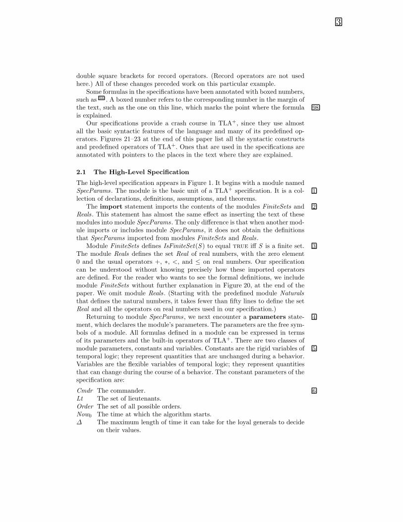
2.1 The High-Level Specification

The high-level specification appears in Figure 1. It begins with a module namedSpecParams . The module is the basic unit of a TLA+ specification. It is a col- 1

lection of declarations, definitions, assumptions, and theorems.The import statement imports the contents of the modules FiniteSets and 2

Reals . This statement has almost the same effect as inserting the text of thesemodules into module SpecParams . The only difference is that when another mod-ule imports or includes module SpecParams , it does not obtain the definitionsthat SpecParams imported from modules FiniteSets and Reals .

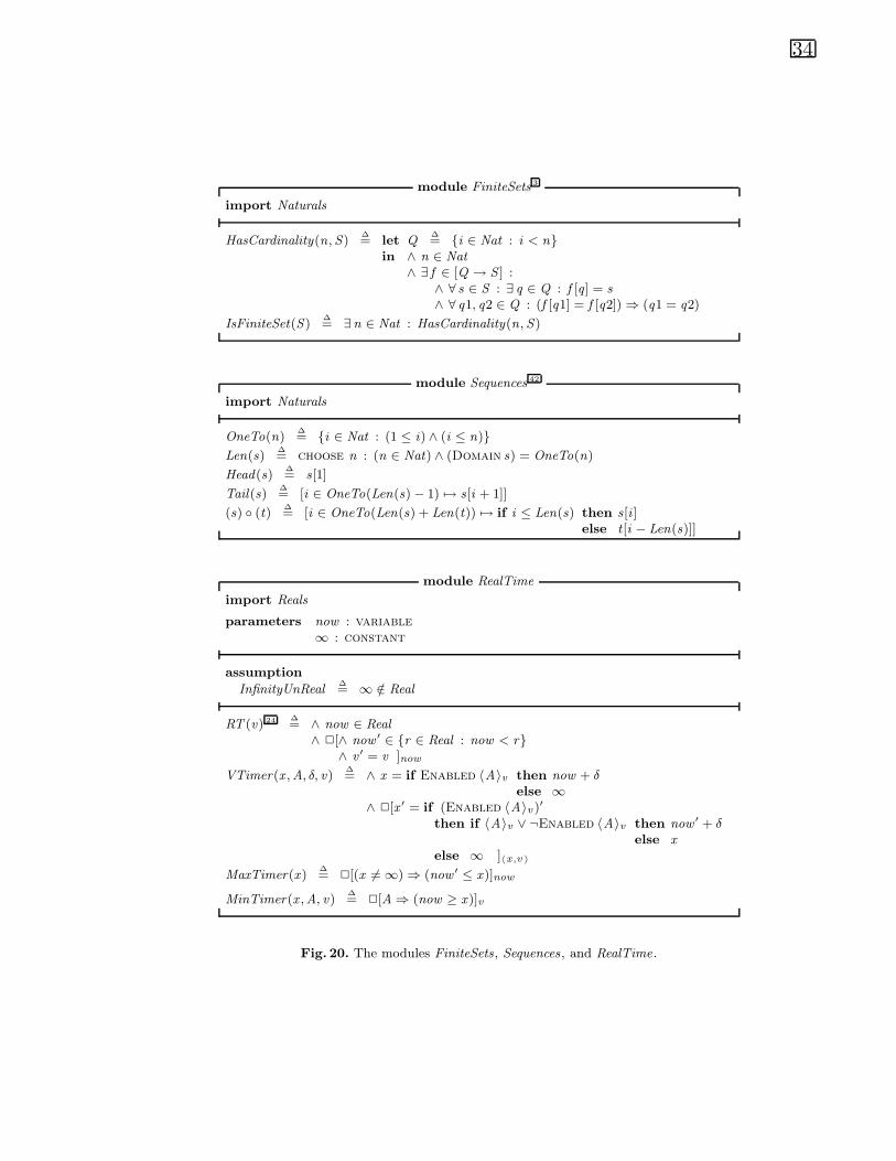
Module FiniteSets defines IsFiniteSet(S ) to equal true iff S is a finite set. 3

The module Reals defines the set Real of real numbers, with the zero element0 and the usual operators +, ∗, <, and ≤ on real numbers. Our specificationcan be understood without knowing precisely how these imported operatorsare defined. For the reader who wants to see the formal definitions, we includemodule FiniteSets without further explanation in Figure 20, at the end of thepaper. We omit module Reals . (Starting with the predefined module Naturalsthat defines the natural numbers, it takes fewer than fifty lines to define the setReal and all the operators on real numbers used in our specification.)

Returning to module SpecParams , we next encounter a parameters state- 4

ment, which declares the module’s parameters. The parameters are the free sym-bols of a module. All formulas defined in a module can be expressed in termsof its parameters and the built-in operators of TLA+. There are two classes ofmodule parameters, constants and variables. Constants are the rigid variables of 5

temporal logic; they represent quantities that are unchanged during a behavior.Variables are the flexible variables of temporal logic; they represent quantitiesthat can change during the course of a behavior. The constant parameters of thespecification are:

Cmdr The commander. 6

Lt The set of lieutenants.Order The set of all possible orders.Now0 The time at which the algorithm starts.∆ The maximum length of time it can take for the loyal generals to decide

on their values.

4

module SpecParams 1

import FiniteSets, Reals 3

parameters Cmdr , Lt ,Order , Now0, ∆6 : constant

status, ord ,now 7 : variable

assumption HiAssump 11 ∆= ∧ (IsFiniteSet(Lt)) ∧ (Cmdr /∈ Lt)∧ “?” /∈ Order∧ Now0 ∈ Real∧ (∆ ∈ Real) ∧ (0 < ∆)

Gen 13 ∆= Lt ∪ {Cmdr}

Loyal(g) 13 ∆= status[g ] = “Loyal”

module HiLevel

import SpecParams, Reals, RealTime

LInit(g) 20 ∆= ∧ status[g ] ∈ {“Loyal”, “Traitor”}∧ Loyal(g)⇒ (ord [g ] = “?”)

CInit 18 ∆= ∧ status[Cmdr ] ∈ {“Loyal”, “Traitor”}∧ Loyal(Cmdr)⇒ (ord [Cmdr ] ∈ Order)

Fail(g) 19 ∆= status′ [g ] = “Traitor”

Choose(g) 21 ∆= ∧ Loyal(g) ∧ (ord [g ] = “?”)∧ ord ′[g ] ∈ Order∧ ∀ h ∈ Gen : Loyal(h)′ ∧ (ord ′[h] �= “?”)⇒ (ord ′[g ] = ord ′[h])∧ unchanged status[g ]

var(g) 18 ∆= 〈ord [g ], status[g ]〉

CSpec 15 ∆= CInit ∧✷[Fail(Cmdr)]var(Cmdr)

LSpec(g) 20 ∆= ∧ LInit(g) ∧ ✷[Choose(g) ∨ Fail(g)]var(g)

∧ ✷(Loyal(g) ∧ (ord [g ] = “?”)⇒ (now ≤ Now0 + ∆))

Spec 23 ∆= ∧ CSpec∧ ∀ g ∈ Lt : LSpec(g)∧ (now = Now0)∧ RT (〈ord , status 〉)

theoremSpecGood 25 ∆

= Spec ⇒ ✷ ∀ g ∈ Gen :Loyal(g) ∧ (Now0 + ∆ < now)⇒ ∧ ord [g ] ∈ Order∧ ∀ h ∈ Gen : Loyal(h)⇒ (ord [g ] = ord [h])

Fig. 1. The high-level specification.

5

The variable parameters are:

status For each general g, the value of status [g] will be the string “Loyal” or 7

“Traitor”, denoting whether or not the general is loyal. (Strings, denotedby expressions of the form “ . . . ”, are a predefined data type of TLA+.)The Byzantine generals problem is expressed in terms of which gener-als are loyal. In the formal specification, the state must describe whichgenerals are loyal. Hence, we introduce the variable status .

ord For each general g, the value of ord [g] denotes the order chosen by generalg, or the string “?” if g has not yet chosen an order.

now The variable now will be a real number that denotes the current time.

In our informal discussion, we describe the values that variables will have in abehavior that satisfies the specification. TLA is a typeless logic, which means thata variable can assume any value. (More precisely, for any value v and variable x ,there is a state in which the value of x is v .) Thus, when we say that the valueof status [g] will be a string, we mean that its value will be a string in every stateof every behavior that satisfies the specification we are about to describe.

The lines are primarily decorative, though the second one serves 8

to delimit the assumption section.An assumption section asserts assumptions about constant parameters. In 9

this module, there is a single assumption named HiAssump, which is definedto be the expression to the right of the ∆= . In general, the symbol ∆= denotes 10

that the identifier to its left is defined to equal the expression to its right. Theformula HiAssump is the conjunction of four assertions: 11

1. Lt (the set of lieutenants) is a finite set that does not contain Cmdr .2. “?” is not a possible order.3. Now0 is a real number.4. ∆ is a positive real number.

TLA+ uses the notation that a list of expressions bulleted by ∧ denotes their 12

conjunction, and a list of expressions bulleted by ∨ denotes their disjunction.Indentation is used to eliminate parentheses.

Following the assumption section is a section consisting of two definitions.The constant operator Gen is defined to be the set of all generals—both the 13

lieutenants and the commander. The boolean operator Loyal is defined so thatLoyal(x ) equals true iff status [x ] equals “Loyal”, for any x . (We care about thevalue of Loyal(x ) only when x is an element of Gen.) Round parentheses denoteapplication of an operator to its argument (or arguments). The symbol Loyal byitself, without an argument, is not a syntactically complete expression. Squarebrackets denote function application. Both status and status [e] are syntacticallycomplete expressions that denote values, for any expression e.

The line ends the module. 14

The actual specification is contained in module HiLevel , which comes next.This module imports the modules SpecParams , Reals , and RealTime.

6

The RealTime module is used to express real-time properties. It is essentiallythe same module as in [15], which in turn used the definitions from [2].1 Speci-fying real-time properties is an engineering problem that is solved by applyingstandard methods. We will explain the operators in the RealTime module asthey appear in our specification. The module is given in Figure 20.

Importing SpecParams provides module HiLevel with the specification pa-rameters and the definitions of Gen and Loyal . Importing SpecParams does notimport the modules FiniteSets and Reals that it in turn imports.

Instead of reading module HiLevel in sequence, we examine next the temporalformula CSpec, which specifies the commander. This formula has the canonical15

form Init ∧ ✷[Next ]v for a process specification2, where

Init is a predicate—a Boolean expression made from constants and variables. Itdescribes the initial state of the process’s variables.

Next is an action—a boolean expression made from constants, variables, andprimed variables. It describes all steps (pairs of successive states) that canchange the process’s variables. In an action, unprimed variables denotevalues in the first (starting) state and primed variables denote values in thesecond (final) state.

v is a state function—a nonboolean expression made from constants and vari-ables. It is usually a tuple that describes all components of the process’sstate.

The formula [Next ]v denotes Next ∨ (v ′ = v), so it represents a step that is16

either a Next step or one that leaves v (and hence all variables in the tuple v)unchanged. The temporal operator ✷ means always, so Init ∧ ✷[Next ]v is true17

for a behavior (infinite sequence of states) iff the first state satisfies Init andevery successive pair of states is either a Next step or leaves v unchanged.

The commander’s state is described by ord [Cmdr ] and status [Cmdr ], whichare the components of the tuple var(Cmdr). (In TLA+, tuples are enclosed in18

angle brackets 〈. . .〉.) The initial condition CInit asserts that

1. The commander’s status is either “Loyal” or “Traitor”.2. If her status is “Loyal”, then her order is an element of Order . The symbol

⇒ denotes logical implication. It has lower precedence (binds more loosely)than any other boolean operator.

The commander’s next-state relation is Fail(Cmdr), which asserts that the new19

value of status [Cmdr ] is “Traitor”. This allows any step that ends in a state withstatus [Cmdr ] equal to “Traitor”. Such a step can change ord [Cmdr ] to any value.Thus, the formula CSpec is satisfied by any behavior that either (i) consists ofan infinite number of states with status [Cmdr ] = “Loyal” and ord [g] = o, forsome o in Order , or (ii) starts with a finite (possibly empty) sequence of such

1 The definition of VTimer in the RealTime module of [15] contains a typographicalerror; the correct definition appears in [2] and Figure 20.

2 Since real-time conditions are used to specify progress, there are no fairness condi-tions in our processes.

7

states and ends with an infinite sequence of states in which status [Cmdr ] equals“Traitor” and ord [Cmdr ] assumes completely arbitrary values.

The formula CSpec describes only the values assumed by ord [Cmdr ] andstatus [Cmdr ]. It makes no assertion about any other part of the state—such asthe value of the variable now , or of ord [g] for g different from Cmdr , or of avariable foo that might be introduced later.

The formula LSpec(g) is the specification of lieutenant g. It is the conjunction 20

of two formulas. The first asserts that LInit(g) holds initially and that each stepis a Choose(g) step, a Fail(g) step, or a step that leaves lieutenant g’s stateunchanged. The initial predicate LInit(g) asserts that (i) status [g] has a correctvalue, and (ii) if g is loyal, then ord [g] equals “?”, denoting that g has not yetchosen an order. A Choose(g) step is one in which 21

1. In the starting a state, g is loyal and has not yet chosen an order. (Any steptaken by a traitorous general can be interpreted as a Fail step.)

2. In the final state, g has chosen an order.3. For every general h that, in the final state, is loyal and has chosen an order,

the order that h has chosen is the same as the one that g has chosen.4. g’s status does not change, which by (1) implies that he is still loyal in the

final state. The formula unchanged f is an abbreviation for f ′ = f . 22

The second conjunct of LSpec(g) is of the form ✷P , for a predicate P . Sucha formula asserts of a behavior that P is true in every state. In this case, theformula asserts that if g is loyal and has not chosen an order, then now is atmost Now0 +∆. In other words, it asserts that if now is greater than Now0 +∆and g is loyal, then he must have chosen an order. Since we interpret now as thecurrent time, the second conjunct of LSpec(g) asserts that if g is loyal, then hemust choose an order by time Now0 + ∆.

The formula Spec is the complete high-level specification. It asserts 23

1. The commander’s specification CSpec.2. The specification LSpec(g), for each lieutenant g.3. now = Now0, which means that the current time initially (at the start of

the algorithm) equals Now0.4. Formula RT (〈ord , status 〉). Module RealTime defines formula RT (v) to as- 24

sert that (a) now is a monotonically nondecreasing real number and (b) stepsthat change now leave v unchanged. Thus, RT (〈ord , status 〉) asserts that(a) now changes the way we expect time to change, and (b) ord and statusdo not change when now does. Thus, in steps that change ord and status , thevalue of now is the same in the initial and final state. Intuitively, this meansthat we are considering changes to ord and status to happen instantaneously.

Formula Spec is the high-level specification. This means that we consider a be-havior to represent a correct execution of the algorithm iff it satisfies Spec. Aspecification is therefore a definition, and a definition cannot be right or wrong.However, a specifications can fail to capture our intent. To gain confidence in aspecification, we can prove theorems about it. Such theorems usually have the

8

form Spec ⇒ Prop, which asserts that every behavior satisfying the specificationSpec also satisfies the property Prop. Module HiLevel asserts such a theorem,named SpecGood . This theorem states that, in any behavior satisfying Spec, it25

is always the case that, for any general g, if g is loyal and the time is later thanNow0+∆, then g has chosen an order and his order is the same as that of everyother loyal general. In other words, every loyal general chooses an order by timeNow0 + ∆, and that order is the same as any other loyal general’s order. Alltheorems are proved in Section 3.

2.2 The Mid-Level Specification

The mid-level specification describes Algorithm OM(1) of [16], an “oral-message”Byzantine agreement algorithm that works in the presence of at most one traitor.It is a two-round algorithm. In the first round, the commander sends her messageto all lieutenants. In the second round, each lieutenant relays the message hereceived to all other lieutenants. A lieutenant chooses his order by applying amajority function to the values that he has received. The only requirements onthis majority function are (i) if the same order o is received from all but one ofthe other generals, then o is chosen, and (ii) all lieutenants use the same majorityfunction.

This informal description is essentially the one given in [16]. It contains sev-eral tacit assumptions—for example, that every lieutenant receives a value in thefirst round, even if the commander is a traitor. The formal specification makesthese assumptions explicit.

Module MidLevelParams of Figure 2 declares the following new parameters26

that are used in the mid-level specification.

rcvd For each lieutenant g, the order that g receives directly from the comman-der is recorded in rcvd [g][g], and the relayed order that g receives fromeach other lieutenant h is recorded in rcvd [g][h]. Thus, for each lieutenantg, the value of rcvd [g] will be a function whose domain is the set Lt oflieutenants. If lieutenant g is loyal, then before any orders have been sent,rcvd [g][h] will equal “?”, for all lieutenants h.

Majority The majority function. More precisely, Majority is an operator with asingle argument. We care about the value of Majority(f ) only when f is afunction from Lt to the set Order of orders.

δ The maximum delay between when an order is sent and when it is received.This delay applies both to the sending of orders by the commander and tothe relaying of orders by the lieutenants. (The delay δ includes the timeneeded to decide to send an order.)

ε The maximum time it takes a lieutenant to make a decision. In this spec-ification, the only decision he has to make is to choose an order once hehas received all the relayed orders.

Assumption MidAssump makes the following assertion about the constant pa-27

rameters.

9

module MidLevelParams

import SpecParams, Realsexport 29 MidLevelParams, SpecParams, Reals

parameters rcvd 26 : variable

Majority( ), δ, ε 26 : constant

assumption

MidAssump 27 ∆= ∧ (δ ∈ Real) ∧ (ε ∈ Real) ∧ (2 ∗ δ + ε ≤ ∆)

∧ ∀ f ∈ [Lt → Order ] 28 :∧ Majority(f ) ∈ Order∧ ∀ o ∈ Order : (∃ h ∈ Lt : ∀ g ∈ Lt \ {h} : f [g ] = o)

⇒ (Majority(f ) = o)

Fig. 2. Module MidLevelParams.

1. δ and ε are real numbers such that 2 ∗ δ + ε is at most ∆.2. For any function f that maps lieutenants to orders:

1. Majority(f ) is an order.2. If o is an order such that f [g] equals o for every lieutenant except some

lieutenant h, then Majority(f ) equals o.The expression [Lt → Order ] denotes the set of all functions f with domain 28

Lt such that f [g] ∈ Order , for all g ∈ Lt .

The export statement causes the named definitions to be imported by any mod- 29

ule that imports MidLevelParams. A module name stands for all definitions fromthat module. (Omitting the export statement would be equivalent to writingexport MidLevelParams .)

Module MidLevel in Figure 3 defines the formula Spec to be the mid-levelspecification. It first imports two other modules. Importing MidLevelParamsimports all its parameters, including the ones it imported from SpecParams .

The include statement incorporates the definitions from module HiLevel , 30

with all defined symbols prefixed by “Hi .”; for example, a definition of Hi .varis included that makes Hi .var(h) equal to 〈ord [h], status [h]〉. Parameters of anincluded module are instantiated by expressions. In the absence of explicit in-stantiation (described below), a parameter is instantiated by the symbol of thesame name. Thus, the parameter Cmdr of HiLevel is instantiated by Cmdr (a pa-rameter of MidLevel , obtained via the import statement); the parameter ord ofHiLevel is instantiated by ord ; etc. When a module is included, its assumptions(with the appropriate instantiations) must be provable from the assumptionsand definitions of the including module. Thus, assumption Hi .HiAssump, theassumption of the included module HiLevel , must be provable from the assump-tions and definitions of module MidLevel . This assumption follows trivially fromassumption HiLevel , which is imported from module MidLevelParams, which inturn imports it from module SpecParams .

10

module MidLevel

import MidLevelParams, RealTimeinclude HiLevel as Hi 30

LInit(g) 32 ∆= ∧ Hi .LInit(g)∧ Loyal(g)⇒ (rcvd [g ] = [h ∈ Lt �→ “?”])

Issue(g) 34 ∆= ∧ Loyal(g) ∧ rcvd [g ][g ] = “?”∧ ∃ o ∈ Order : ∧ rcvd ′[g ] = [rcvd [g ] except ![g ] = o]

∧ Loyal(Cmdr)⇒ (o = ord [Cmdr ])∧ unchanged 〈ord [g ], status[g ]〉

Relay(g , h) 35 ∆= ∧ Loyal(g) ∧ rcvd [g ][h] = “?”∧ ∃ o ∈ Order : ∧ rcvd ′[g ] = [rcvd [g ] except ![h] = o]

∧ Loyal(h)⇒ (o = rcvd [h][h])∧ unchanged 〈ord [g ], status[g ]〉

Choose(g)∆= ∧ Loyal(g) ∧ ord [g ] = “?”∧ ∀ h ∈ Lt : rcvd [g ][h] �= “?”∧ ord ′[g ] = Majority(rcvd [g ])∧ unchanged 〈rcvd [g ], status[g ]〉

Next(g) 33 ∆= Issue(g) ∨ (∃ h ∈ Lt \ {g} : Relay(g , h)) ∨ Choose(g) ∨ Hi .Fail(g) 36

var(g)∆= 〈ord [g ], rcvd [g ], status[g ]〉

LSpec(g)∆= ∧ LInit(g) ∧ ✷[Next(g)] 32var(g)

∧ ✷(Loyal(g) ∧ (rcvd [g ][g ] = “?”)⇒ (now ≤ Now0 + δ)) 37

∧ ∀ h ∈ Lt \ {g} :

✷(Loyal(g) ∧ (rcvd [g ][h] = “?”)⇒ (now ≤ Now0 + 2 ∗ δ)) 37

∧ ∃∃∃∃∃∃ t : ∧ VTimer(t , Choose(g), ε, var(g))

∧ MaxTimer(t) 38

Spec 31 ∆= ∧ Hi .CSpec∧ ∀ g ∈ Lt : LSpec(g)∧ now = Now0

∧ RT (〈ord , rcvd , status 〉)

OneTraitor 40 ∆= ∃ h ∈ Gen : ∀ g ∈ Gen \ {h} : Loyal(g)

theoremMidCorrect 40 ∆

= (✷OneTraitor) ∧ Spec ⇒ Hi .Spec

Fig. 3. Module MidLevel

11

Formula Spec is the specification of the mid-level algorithm. It is similar to 31

the specification Spec of module HiLevel , consisting of the conjunction of fourformulas that assert: (i) the specification Hi .CSpec of the commander includedfrom module HiLevel , (ii) formula LSpec(g), for every lieutenant g, (iii) now isinitially equal to Now0, and (iv) formula RT (〈ord , rcvd , status 〉). As explained inSection 2.1, RT (〈ord , rcvd , status 〉) asserts that now behaves the way we expectit to and that ord , rcvd , and status change instantaneously. The rest of thespecification involves the definition of LSpec(g), the specification of lieutenant g.Formula LSpec(g) is the conjunction of four formulas, which we describe in turn.

The first conjunct of LSpec(g) has the canonical form Init ∧ ✷[Next ]v ex- 32

plained in Section 2.1. The initial predicate LInit(g) asserts (i) the initial condi-tion Hi .LInit(g) on status [g] and ord [g] and (ii) that rcvd [g] is a function withdomain Lt such that rcvd [g][h] equals “?” for every h in Lt . In general, theconstruct [x ∈ S → exp(x )] denotes the function f with domain S such thatf [x ] = exp(x ) for all x in S . The next-state relation Next(g) is the disjunction 33

of four actions:

Issue(g) Represents the sending of an order by the commander to lieutenant g. 34

It is enabled iff g is loyal and rcvd [g][g] equals “?”, denoting that ghas not yet received an order from the commander. The action setsrcvd [g][g] to an order that, if the commander is loyal, is actually herorder. The notation [f except ! [x ] = exp] denotes a function f thatis the same as f except that f [x ] equals exp.

∃ h ∈ Lt\{g} : Relay(g, h) Asserts that a Relay(g, h) step occurs, for some lieu- 35

tenant h other than g. Such a step represents the relaying of an orderfrom h to g. If h is loyal, then the relayed order is rcvd [h][h].

Hi .Fail(g) As described above, an action taken when g is or becomes a traitor. 36

It allows arbitrary changes to ord [g] and rcvd [g] (and all variablesother than status [g]).

Choose(g) The action in which g chooses his order by applying Majority to hisarray rcvd [g] of relayed values.

The final three conjuncts of LSpec(g) place timing bounds on when g’s actionsmust occur. The second conjunct asserts that (it is always true that) if g is loyal 37

and rcvd [g][g] equals “?”, then now is at most Now0 + δ. If g is loyal, rcvd [g][g]equals “?” iff an Issue(g) step has not occurred. Thus, this conjunct asserts that,if g is loyal, then an Issue(g) step must occur by time Now0 + δ. Similarly, thethird conjunct asserts that, if g is loyal, then a Relay(g, h) step must occur bytime Now0 + 2 ∗ δ.

The final conjunct of LSpec(g) places a timing bound on the Choose(g) ac-tion, using the temporal formulas VTimer and MaxTimer , defined in module 38

RealTime. These formulas were introduced in [2] and used again in [15] as ageneral method for specifying real-time bounds. If A is an action and v a statefunction such that any A step changes v , and if t is a variable that does notoccur in A or v , then the formula VTimer(t ,A, ε, v) ∧ MaxTimer(t) asserts thatA cannot be enabled for more than ε time units before the next A step occurs.

12

The temporal existential quantifier ∃∃∃∃∃∃ t essentially hides the variable t . Thus, the 39

fourth conjunct of LSpec(g) asserts that, if lieutenant g is loyal, then a Choose(g)step must occur within ε time units of when he has received an order from thecommander and from all other lieutenants.

Finally, the module asserts the correctness of the mid-level algorithm. The40

predicate OneTraitor asserts of a state that there is at most one traitorousgeneral. Theorem MidCorrect asserts that, for any behavior, if (i) there is alwaysat most one traitorous general and (ii) formula Spec holds, then formula Hi .Specholds. In other words, this theorem asserts that, in the presence of at most onetraitor, the mid-level specification implements the high-level specification.

2.3 The Low-Level Specification

In the mid-level specification, a value is transferred from the commander to alieutenant in a single step, and is relayed from one lieutenant to another in asingle step. In the low-level specification, we model the way values are transmit-ted over communication channels. This requires adding timeouts to detect if atraitorous general fails to send a message.

The specification uses module TimedChannel of Figure 4, which provides41

generic definitions for describing the transmission of values over a channel. Thismodule imports module Sequences to define operators on sequences. In TLA+,an n-tuple 〈v1, . . . , vn 〉 is a function whose domain is the set {1, . . . ,n} of nat-42

ural numbers, where 〈v1, . . . , vn 〉[i ] equals v i , for 1 ≤ i ≤ n. The Sequencesmodule represents sequences as tuples. The module is given without explanationin Figure 20. It defines the usual operators Head , Tail , and ◦ (concatenation)on sequences.

Module TimedChannel has two variable parameters:43

src The interface at the sender’s end of the channel. It will be a pair whosefirst element is a sequence of values and whose second element is either 0or 1.

dest The interface at the receiver’s end of the channel. It will be a pair whosefirst element is a sequence of values and whose second element is either 0or 1.

(The purpose of the second components of src and dest is explained below.) Themodule has a single constant parameter τ , which is a real number that representsthe maximum time required to transmit one value.

The sending of a value v is initiated by a Send(v) step, which appends v44

to the tail of src[1] and complements src[2]—changing its value from 0 to 1 orvice-versa. Receipt of the value v occurs with a Rcv(v) step, which is enabled iffv is the head of the sequence dest [1]. A Rcv(v) step removes v from the head ofdest [1] and complements dest [2].

The transmission of a value from one end of the channel to the other is45

modeled by a Tmt step, which moves an element from the head of src[1] to thetail of dest [1].

13

module TimedChannel 41

import Sequences, Reals, RealTime

parameters src, dest 43 : variable

τ 47 : constant

assumption Assump∆= (τ ∈ Real) ∧ (0 < τ )

Send(v) 44 ∆= src′ = 〈src[1] ◦ 〈v 〉, 1− src[2]〉

Rcv(v) 44 ∆= ∧ (dest [1] �= 〈 〉) ∧ (v = Head(dest [1]))∧ dest ′ = 〈Tail(dest [1]), 1− dest [2]〉

Tmt 45 ∆= ∧ src[1] �= 〈 〉∧ src′ = 〈Tail(src[1]), src[2]〉∧ dest ′ = 〈dest [1] ◦ 〈Head(src[1])〉, dest [2]〉

ext 48 ∆= 〈src[2], dest [2]〉

Spec 46 ∆= ∧ (src = 〈〈 〉, 0〉) ∧ ✷[Tmt ∨ ∃ v : Send(v)]src∧ (dest = 〈〈 〉, 0〉) ∧ ✷[Tmt ∨ ∃ v : Rcv(v)]dest∧ ∃∃∃∃∃∃ t : VTimer(t ,Tmt , τ, 〈src, dest 〉) ∧MaxTimer(t) 47

Fig. 4. Module TimedChannel .

Formula Spec is the specification of the timed channel. A behavior satisfies46

this formula iff the variables src and dest behave the way they should for a timedchannel. The formula has three conjuncts. The first describes the sequence ofvalues assumed by src. Initially, src[1] is the empty sequence and src[2] equals0; every step that changes src is a Tmt step or a Send(v) step, for some v . Thesecond conjunct similarly describes the sequence of values assumed by dest . Thethird conjunct asserts the real-time requirement. As explained in Section 2.2, theconjunct asserts that Tmt cannot remain enabled for more than τ time units 47

before the next Tmt step occurs. Thus, this conjunct asserts that, when src[1]is nonempty, values are moved from it to dest [1] at the rate of at least one everyτ time units.

We now come to ext , the pair consisting of the second components of src and 48

dest , and the explanation of what those second components are for. The channelspecification Spec allows arbitrary values to be sent “spontaneously”, and itallows those values to be received at arbitrary times. This specification is usedby conjoining it with specifications of a sender and receiver that constrain whenSend and Rcv actions occur. The sender’s specification will describe when Sendactions can occur and what values they can send; the receiver’s specification willdescribe when Rcv actions can occur. The sender’s and receiver’s specificationsmust also allow the channel’s internal Tmt steps. They allow such steps byallowing any step that leave ext unchanged; Spec implies that any such stepmust be a Tmt step.

Module LowLevelParams in Figure 5 begins the specification of the low-level

14

module LowLevelParams

import SpecParams, MidLevelParams, Realsexport SpecParams, MidLevelParams, Reals, LowLevelParams, Hi, Mid, TC 52

parameters in, out , sent 49 : variable

τ 50 : constant

assumption LowAssump∆= (τ ∈ Real) ∧ (0 < τ ) ∧ (τ + 3 ∗ ε ≤ δ)

include HiLevel as Hiinclude MidLevel as Midinclude TimedChannel as TC (g ,h) with src ← out [g ][h], dest ← in[h][g ] 51

AllBut(func, g) 53 ∆= [h ∈ Lt \ {g} �→ func[h]]

NotSent(g , h)∆= sent [g ][h] = “No”

ext(g) 54 ∆= [h ∈ Lt �→ TC (g , h).ext ]

Fig. 5. Module LowLevelParams.

algorithm itself. The module imports the two higher-level . . .Params modulesand declares three new variable parameters:

in The state function in[h][g] represents the receiver’s end (dest) of the chan-49

nel from g to h.out The state function out [g][h] represents the sender’s end (src) of the channel

from g to h.sent The value of sent [g][h], which will be either “Yes” or “No”, records whether

or not general g has sent a value to lieutenant h. For each general g, sent [g]will be a function with domain Lt .

The constant parameter τ has the same meaning as in module TimedChannel .50

The module next asserts assumption LowAssump, which relates τ to δ andε. The module also asserts assumptions HiAssump and MidAssump, which areimported with modules SpecParams and MidLevelParams, respectively.

Module LowLevelParams then includes modules HiLevel and MidLevel , andincludes a parameterized copy of module TimedChannel . The latter include51

statement incorporates all the definitions from module TimedChannel prefixedwith “TC (g, h).”, and with the indicated instantiations of the parameters srcand dest . For example, it includes the definition

TC (g, h).Tmt ∆= ∧ out [g][h][1] �= 〈 〉∧ out [g][h]′ = 〈Tail(out [g][h][1]), out [g][h][2]〉∧ in[h][g]′ = 〈in[h][g][1] ◦ 〈Head(out [g][h][1])〉, in[h][g][2]〉

The export statement exports all these included definitions, as well as the ones52

15

from the imported modules and the definitions made in the LowLevelParamsmodule itself.

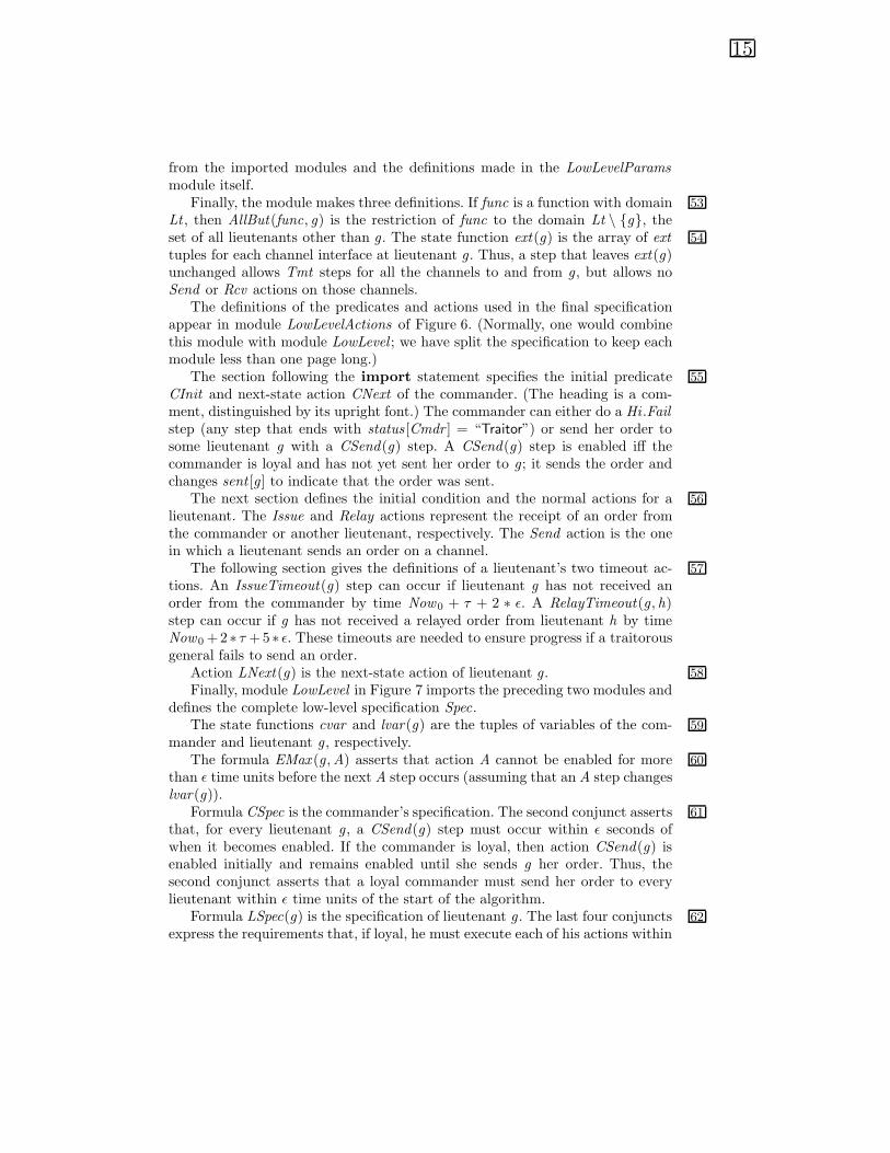
Finally, the module makes three definitions. If func is a function with domain 53

Lt , then AllBut(func, g) is the restriction of func to the domain Lt \ {g}, theset of all lieutenants other than g. The state function ext(g) is the array of ext 54

tuples for each channel interface at lieutenant g. Thus, a step that leaves ext(g)unchanged allows Tmt steps for all the channels to and from g, but allows noSend or Rcv actions on those channels.

The definitions of the predicates and actions used in the final specificationappear in module LowLevelActions of Figure 6. (Normally, one would combinethis module with module LowLevel ; we have split the specification to keep eachmodule less than one page long.)

The section following the import statement specifies the initial predicate 55

CInit and next-state action CNext of the commander. (The heading is a com-ment, distinguished by its upright font.) The commander can either do a Hi .Failstep (any step that ends with status [Cmdr ] = “Traitor”) or send her order tosome lieutenant g with a CSend(g) step. A CSend(g) step is enabled iff thecommander is loyal and has not yet sent her order to g; it sends the order andchanges sent [g] to indicate that the order was sent.

The next section defines the initial condition and the normal actions for a 56

lieutenant. The Issue and Relay actions represent the receipt of an order fromthe commander or another lieutenant, respectively. The Send action is the onein which a lieutenant sends an order on a channel.

The following section gives the definitions of a lieutenant’s two timeout ac- 57

tions. An IssueTimeout(g) step can occur if lieutenant g has not received anorder from the commander by time Now0 + τ + 2 ∗ ε. A RelayTimeout(g, h)step can occur if g has not received a relayed order from lieutenant h by timeNow0 +2 ∗ τ +5 ∗ ε. These timeouts are needed to ensure progress if a traitorousgeneral fails to send an order.

Action LNext(g) is the next-state action of lieutenant g. 58

Finally, module LowLevel in Figure 7 imports the preceding two modules anddefines the complete low-level specification Spec.

The state functions cvar and lvar(g) are the tuples of variables of the com- 59

mander and lieutenant g, respectively.The formula EMax (g,A) asserts that action A cannot be enabled for more 60

than ε time units before the next A step occurs (assuming that an A step changeslvar(g)).

Formula CSpec is the commander’s specification. The second conjunct asserts 61

that, for every lieutenant g, a CSend(g) step must occur within ε seconds ofwhen it becomes enabled. If the commander is loyal, then action CSend(g) isenabled initially and remains enabled until she sends g her order. Thus, thesecond conjunct asserts that a loyal commander must send her order to everylieutenant within ε time units of the start of the algorithm.

Formula LSpec(g) is the specification of lieutenant g. The last four conjuncts 62

express the requirements that, if loyal, he must execute each of his actions within

16

module LowLevelActions

import LowLevelParams, RealTime

CInit∆= ∧ Hi .CInit∧ Loyal(Cmdr)⇒ (sent [Cmdr ] = [h ∈ Lt �→ “No”])

The commander. 55

CSend(g)∆= ∧ Loyal(Cmdr) ∧NotSent(Cmdr , g)∧ TC (Cmdr , g).Send(ord [Cmdr ])∧ sent ′[Cmdr ] = [sent [Cmdr ] except ![g ] = “Yes”]∧ unchanged 〈in[Cmdr ],AllBut(out [Cmdr ], g), ord [Cmdr ],

status[Cmdr ]〉CNext

∆= Hi .Fail(Cmdr) ∨ ∃ g ∈ Lt : CSend(g)

LInit(g)∆= ∧ Mid .LInit(g)∧ Loyal(g)⇒ (sent [g ] = [h ∈ Lt �→ “No”])

Lieutenant g. 56

Issue(g)∆= ∧ Loyal(g) ∧ (rcvd [g ][g ] = “?”)∧ ∃ o ∈ Order : ∧ TC (Cmdr , g).Rcv(o)

∧ rcvd ′[g ] = [rcvd [g ] except ![g ] = o]∧ unchanged 〈ord [g ], AllBut(in[g ],Cmdr), out [g ], status[g ], sent [g ]〉

Send(g , h)∆= ∧ Loyal(g) ∧ (rcvd [g ][g ] �= “?”) ∧NotSent(g , h)∧ TC (g ,h).Send(rcvd [g ][g ])∧ sent ′[g ] = [sent [g ] except ![h] = “Yes”]∧ unchanged 〈ord [g ], rcvd [g ], in[g ],AllBut(out [g ], h), status[g ]〉

Relay(g , h)∆= ∧ Loyal(g) ∧ (rcvd [g ][h] = “?”)∧ ∃ o ∈ Order : ∧ TC (h, g).Rcv(o)

∧ rcvd ′[g ] = [rcvd [g ] except ![h] = o]∧ unchanged 〈ord [g ], AllBut(in[g ], h), out [g ], status[g ], sent [g ]〉

Choose(g)∆= Mid .Choose(g) ∧ unchanged 〈in[g ], out [g ]〉

IssueTimeout(g)∆= ∧ Loyal(g) ∧ (rcvd [g ][g ] = “?”)∧ Now0 + τ + 2 ∗ ε < now∧ ∃ o ∈ Order : rcvd ′[g ] = [rcvd [g ] except ![g ] = o]∧ unchanged 〈ord [g ], in[g ], out [g ], status[g ], sent [g ]〉

Timeout actions. 57

RelayTimeout(g , h)∆= ∧ Loyal(g) ∧ (rcvd [g ][h] = “?”)∧ Now0 + 2 ∗ τ + 5 ∗ ε < now∧ ∃ o ∈ Order : rcvd ′[g ] = [rcvd [g ] except ![h] = o]∧ unchanged 〈ord [g ], in[g ], out [g ], status[g ]〉

LNext(g) 58 ∆= ∨ Issue(g) ∨ Choose(g) ∨ IssueTimeout(g)∨ ∃ h ∈ Lt \ {g} : Send(g , h) ∨ Relay(g , h) ∨ RelayTimeout(g , h)∨ Hi .Fail(g)

Fig. 6. Module LowLevelActions.

17

module LowLevel

import LowLevelParams, LowLevelActions

cvar∆= 〈ord [Cmdr ], ext(Cmdr), status[Cmdr ], sent [Cmdr ]〉 State functions. 59

lvar(g)∆= 〈ord [g ], rcvd [g ], ext(g), status[g ], sent [g ]〉

EMax(g , A) 60 ∆= ∃∃∃∃∃∃ t : VTimer(t , A, ε, lvar(g)) ∧MaxTimer(t)

Temporal formulas.

CSpec 61 ∆= ∧ CInit ∧✷[CNext ]cvar∧ ∀ g ∈ Lt : EMax(Cmdr , CSend(g))

LSpec(g) 62 ∆= ∧ LInit(g) ∧ ✷[LNext(g)]lvar(g)

∧ EMax(g , Issue(g))∧ EMax(g , IssueTimeout(g))∧ EMax(g ,Choose(g))∧ ∀ h ∈ Lt \ {g} : ∧ EMax(g ,Send(g , h))

∧ EMax(g ,Relay(g , h))∧ EMax(g ,RelayTimeout(g , h))

Spec 63 ∆= ∧ CSpec∧ ∀ g ∈ Lt : LSpec(g)∧ ∀ g , h ∈ Gen : TC (g ,h).Spec∧ now = Now0

∧ RT (〈ord , rcvd , in, out , status, sent 〉)

theorem LowCorrect∆= Spec ⇒ Mid .Spec

Fig. 7. Module LowLevel .

18

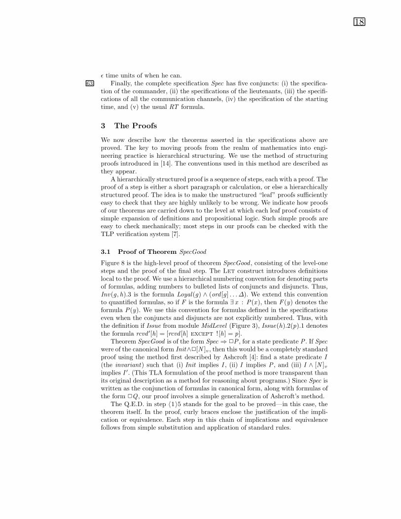
ε time units of when he can.Finally, the complete specification Spec has five conjuncts: (i) the specifica-63

tion of the commander, (ii) the specifications of the lieutenants, (iii) the specifi-cations of all the communication channels, (iv) the specification of the startingtime, and (v) the usual RT formula.

3 The Proofs

We now describe how the theorems asserted in the specifications above areproved. The key to moving proofs from the realm of mathematics into engi-neering practice is hierarchical structuring. We use the method of structuringproofs introduced in [14]. The conventions used in this method are described asthey appear.

A hierarchically structured proof is a sequence of steps, each with a proof. Theproof of a step is either a short paragraph or calculation, or else a hierarchicallystructured proof. The idea is to make the unstructured “leaf” proofs sufficientlyeasy to check that they are highly unlikely to be wrong. We indicate how proofsof our theorems are carried down to the level at which each leaf proof consists ofsimple expansion of definitions and propositional logic. Such simple proofs areeasy to check mechanically; most steps in our proofs can be checked with theTLP verification system [7].

3.1 Proof of Theorem SpecGood

Figure 8 is the high-level proof of theorem SpecGood , consisting of the level-onesteps and the proof of the final step. The Let construct introduces definitionslocal to the proof. We use a hierarchical numbering convention for denoting partsof formulas, adding numbers to bulleted lists of conjuncts and disjuncts. Thus,Inv(g, h).3 is the formula Loyal(g) ∧ (ord [g] . . . ∆). We extend this conventionto quantified formulas, so if F is the formula ∃ x : P(x ), then F (y) denotes theformula P(y). We use this convention for formulas defined in the specificationseven when the conjuncts and disjuncts are not explicitly numbered. Thus, withthe definition if Issue from module MidLevel (Figure 3), Issue(h).2(p).1 denotesthe formula rcvd ′[h] = [rcvd [h] except ! [h] = p].

Theorem SpecGood is of the form Spec ⇒ ✷P , for a state predicate P . If Specwere of the canonical form Init∧✷[N ]v , then this would be a completely standardproof using the method first described by Ashcroft [4]: find a state predicate I(the invariant) such that (i) Init implies I , (ii) I implies P , and (iii) I ∧ [N ]vimplies I ′. (This TLA formulation of the proof method is more transparent thanits original description as a method for reasoning about programs.) Since Spec iswritten as the conjunction of formulas in canonical form, along with formulas ofthe form ✷Q , our proof involves a simple generalization of Ashcroft’s method.

The Q.E.D. in step 〈1〉5 stands for the goal to be proved—in this case, thetheorem itself. In the proof, curly braces enclose the justification of the impli-cation or equivalence. Each step in this chain of implications and equivalencefollows from simple substitution and application of standard rules.

19

Let: Good(g)∆= Loyal(g) ∧ (Now0 + ∆ < now)

⇒ ∧ ord [g ] ∈ Order∧ ∀ h ∈ Gen : Loyal(h)⇒ (ord [g ] = ord [h])

Theorem Spec ⇒ ✷(∀ g ∈ Gen : Good(g))

Let: Inv(g , h)∆= 1.∧ Loyal(g)⇒ ord [g ] ∈ Order ∪ {“?”}

2.∧ Loyal(g) ∧ Loyal(h) ∧ (ord [g ] �= “?”) ∧ (ord [h] �= “?”)⇒ (ord [g ] = ord [h])

3.∧ Loyal(g) ∧ (ord [g ] = “?”)⇒ (now ≤ Now0 +∆)

CInv∆= Loyal(Cmdr)⇒ (ord [Cmdr ] ∈ Order)

〈1〉1. Assume: g , h ∈ LtProve: LSpec(g) ∧ LSpec(h) ⇒ ✷Inv(g , h)

〈1〉2. Assume: g ∈ LtProve: LSpec(g) ∧ CSpec ⇒ ✷Inv(g ,Cmdr)

〈1〉3. CSpec ⇒ ✷CInv

〈1〉4. CInv ∧ (∀ g ∈ Lt : ∀ h ∈ Gen : Inv(g , h))⇒ (∀ g ∈ Gen : Good(g))

〈1〉5. Q.E.D.

Proof: Spec ⇒ {By the definition of Spec.}CSpec ∧ (∀ g , h ∈ Lt : LSpec(g) ∧ LSpec(h))

⇒ {By 〈1〉1, 〈1〉2, and 〈1〉3.}✷CInv ∧ (∀ g , h ∈ Lt : ✷Inv(g , h) ∧✷Inv(g ,Cmdr))

≡ {By the temporal logic rule that ✷ distributes over conjunction.}✷(CInv ∧ (∀ g , h ∈ Lt : Inv(g , h) ∧ Inv(g ,Cmdr))

⇒ {〈1〉4, the definition of Gen, and the temporal logic rule(P ⇒ Q) � (✷P ⇒ ✷Q).}

✷(∀ g ∈ Gen : Good(g))

Fig. 8. The high-level structure of the proof of theorem SpecGood

To finish the proof, we must now prove statements 〈1〉1–〈1〉4. The proof of〈1〉4 involves simple predicate logic and will not be discussed. The proofs of〈1〉1, 〈1〉2, and 〈1〉3 are similar; we consider only 〈1〉1.

The first-level proof of 〈1〉1 appears in Figure 9. The rule that underlies theproof is that proving I ∧ A ⇒ I ′ allows us to infer I ∧ ✷A ⇒ ✷I , where I isa predicate and A an action. This is an RTLA [13] rule, where RTLA is a logicthat is like TLA except that ✷A is an RTLA formula for any action A, not justfor actions A of the form [N ]v . In RTLA, temporal quantification (the operator∃∃∃∃∃∃ ) can be applied only to a TLA formula, not to an arbitrary RTLA formula.All TLA proof rules are valid for RTLA.

To complete the proof of 〈1〉1, we must prove 〈2〉1 and 〈2〉2. Step 〈2〉1 followsfrom the definitions by simple predicate logic. The proof of 〈2〉2 is shown inFigure 10. The proof goal is first transformed into an Assume/Prove form, sothe new goal becomes simply Inv(g, h)′. Inside the proof, these four assumptionsare referred to as assumption 〈2〉:1–〈2〉:4.

Since Inv(g, h) is the conjunction of the formulas Inv(g, h).1, Inv(g, h).2,and Inv(g, h).3, the next level of the proof (steps 〈3〉1–〈3〉4) is immediate. The

20

〈1〉1. Assume: g , h ∈ LtProve: LSpec(g) ∧ LSpec(h)⇒ ✷Inv(g , h)

Let: T (g)∆= Loyal(g) ∧ (ord [g ] = “?”)⇒ (now ≤ Now0 + ∆)

〈2〉1. LInit(g) ∧ LInit(h) ∧ T (g)⇒ Inv(g , h)

〈2〉2. ∧ Inv(g , h)∧ [Choose(g) ∨ Fail(g)]var(g) ∧ [Choose(h) ∨ Fail(h)]var(h)

∧ T (g)′

⇒ Inv(g , h)′

〈2〉3. Q.E.D.

Proof:LSpec(g) ∧ LSpec(h)⇒ {By definition of LSpec and T .}∧ LInit(g) ∧ LInit(h)∧ ✷[Choose(g) ∨ Fail(g)]var(g) ∧✷[Choose(h) ∨ Fail(h)]var(h)

∧ ✷T (g)

⇒ {Using the RTLA rule � ✷P ≡ P ∧✷P ′, for any predicate P .}∧ LInit(g) ∧ LInit(h) ∧ T (g)∧ ✷[Choose(g) ∨ Fail(g)]var(g) ∧✷[Choose(h) ∨ Fail(h)]var(h)

∧ ✷T (g)′

⇒ {By 〈2〉1.}∧ Inv(g , h)∧ ✷[Choose(g) ∨ Fail(g)]var(g) ∧✷[Choose(h) ∨ Fail(h)]var(h)

∧ ✷T (g)′

⇒ {Using the rule that ✷ distributes over ∧.}∧ Inv(g , h)∧ ✷([Choose(g) ∨ Fail(g)]var(g) ∧ [Choose(h) ∨ Fail(h)]var(h) ∧ T (g)′)

⇒ {By 〈2〉2 and the RTLA Rule (I ∧ A⇒ I ′) � (I ∧ ✷A⇒ ✷I ), forany predicate I and action A.}

✷Inv(g , h)

Fig. 9. The high-level structure of the proof of step 〈1〉1 from Figure 8.

21

〈2〉2. ∧ Inv(g , h)∧ [Choose(g) ∨ Fail(g)]var(g) ∧ [Choose(h) ∨ Fail(h)]var(h)

∧ T (g)′

⇒ Inv(g , h)′

Proof: By propositional logic, it suffices to:Assume: 1. Inv(g , h)

2. [Choose(g) ∨ Fail(g)]var(g)

3. [Choose(h) ∨ Fail(h)]var(h)

4. T (g)′

Prove: Inv(g , h)′

〈3〉1. Inv(g , h).1′

Proof: By definition of Inv(g , h).1′ and propositional logic, it suffices to:Assume: Loyal(g)′

Prove: ord ′[g ] ∈ Order ∪ {“?”}〈4〉1. Case: unchanged var(g)

Proof: Assumption 〈2〉:1, Case Assumption 〈4〉, and the definition of Inv , sinceunchanged var(g) implies ord ′[g ] = ord [g ].

〈4〉2. Case: Choose(g)Proof: Case Assumption 〈4〉, since Choose(g).2

∆= ord ′[g ] ∈ Order .

〈4〉3. Case: Fail(g)Proof: Case Assumption 〈4〉 and Assumption 〈3〉 lead to a contradiction, sinceFail(g) implies ¬Loyal(g)′ by definition of Fail and Loyal .

〈4〉4. Q.E.D.Proof: By propositional logic from 〈4〉1, 〈4〉2, 〈4〉3, and Assumption 〈2〉:2,since [A]v

∆= A ∨ (unchanged v).

〈3〉2. Inv(g , h).2′

〈3〉3. Inv(g , h).3′

〈3〉4. Q.E.D.

Proof: 〈3〉1, 〈3〉2, 〈3〉3, and the definition of Inv .

Fig. 10. The proof of step 〈2〉2 from Figure 9.

proof of 〈3〉1 is given; the proofs of 〈3〉2 and 〈3〉3 are analogous.The goal, Inv(g, h).1′ is deduced from assumptions 〈2〉:1 and 〈2〉:2. Since

assumption 〈2〉:2 is a disjunction, we do a proof by cases. The statement Case: Sis equivalent to Assume: S, Prove: Q.E.D.

3.2 Proof of Theorem MidCorrect

Theorem MidCorrect asserts that (✷OneTraitor) ∧ Spec implies Hi .Spec. It istrivial to prove that Spec implies Hi .Spec.1 and Hi .Spec.3, so the problem is prov-ing Hi .Spec.2 and Hi .Spec.4. Proving Hi .Spec.2 requires proving Hi .LSpec(g).1and Hi .LSpec(g).2 for each lieutenant g.

The high-level structure of the proof of theorem MidCorrect appears in Fig-ure 11. Steps 〈1〉2 and 〈1〉4 prove Hi .LSpec(g).1 and Hi .LSpec(g).2, respectively,and 〈1〉5 proves Hi .Spec.4. Steps 〈1〉1 and 〈1〉3 establish useful invariants.

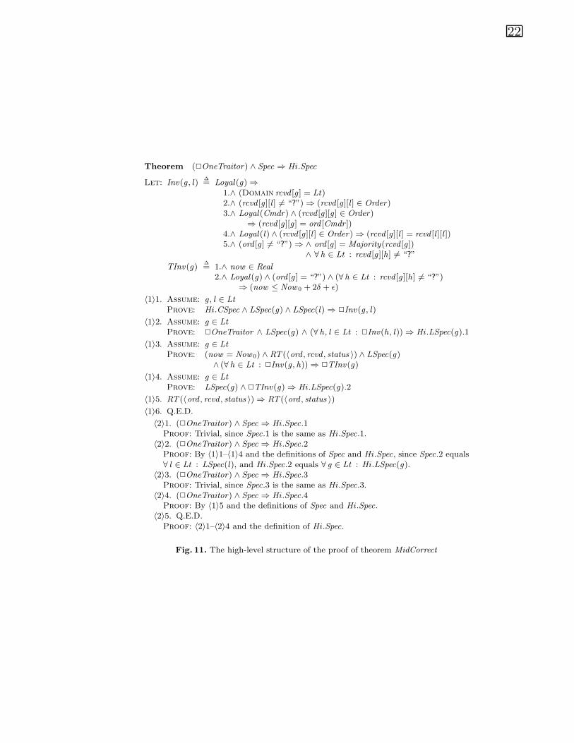
22

Theorem (✷OneTraitor) ∧ Spec ⇒ Hi .Spec

Let: Inv(g , l)∆= Loyal(g)⇒

1.∧ (Domain rcvd [g ] = Lt)2.∧ (rcvd [g ][l ] �= “?”)⇒ (rcvd [g ][l ] ∈ Order)3.∧ Loyal(Cmdr) ∧ (rcvd [g ][g ] ∈ Order)

⇒ (rcvd [g ][g ] = ord [Cmdr ])4.∧ Loyal(l) ∧ (rcvd [g ][l ] ∈ Order)⇒ (rcvd [g ][l ] = rcvd [l ][l ])5.∧ (ord [g ] �= “?”)⇒ ∧ ord [g ] = Majority(rcvd [g ])

∧ ∀ h ∈ Lt : rcvd [g ][h] �= “?”

TInv(g)∆= 1.∧ now ∈ Real

2.∧ Loyal(g) ∧ (ord [g ] = “?”) ∧ (∀ h ∈ Lt : rcvd [g ][h] �= “?”)⇒ (now ≤ Now0 + 2δ + ε)

〈1〉1. Assume: g , l ∈ LtProve: Hi .CSpec ∧ LSpec(g) ∧ LSpec(l)⇒ ✷Inv(g , l)

〈1〉2. Assume: g ∈ LtProve: ✷OneTraitor ∧ LSpec(g) ∧ (∀ h, l ∈ Lt : ✷Inv(h, l))⇒ Hi .LSpec(g).1

〈1〉3. Assume: g ∈ LtProve: (now = Now0) ∧ RT (〈ord , rcvd , status 〉) ∧ LSpec(g)

∧ (∀ h ∈ Lt : ✷Inv(g , h))⇒ ✷TInv(g)

〈1〉4. Assume: g ∈ LtProve: LSpec(g) ∧✷TInv(g)⇒ Hi .LSpec(g).2

〈1〉5. RT (〈ord , rcvd , status 〉)⇒ RT (〈ord , status 〉)〈1〉6. Q.E.D.

〈2〉1. (✷OneTraitor) ∧ Spec ⇒ Hi .Spec.1Proof: Trivial, since Spec.1 is the same as Hi .Spec.1.

〈2〉2. (✷OneTraitor) ∧ Spec ⇒ Hi .Spec.2Proof: By 〈1〉1–〈1〉4 and the definitions of Spec and Hi .Spec, since Spec.2 equals∀ l ∈ Lt : LSpec(l), and Hi .Spec.2 equals ∀ g ∈ Lt : Hi .LSpec(g).

〈2〉3. (✷OneTraitor) ∧ Spec ⇒ Hi .Spec.3Proof: Trivial, since Spec.3 is the same as Hi .Spec.3.

〈2〉4. (✷OneTraitor) ∧ Spec ⇒ Hi .Spec.4Proof: By 〈1〉5 and the definitions of Spec and Hi .Spec.

〈2〉5. Q.E.D.Proof: 〈2〉1–〈2〉4 and the definition of Hi .Spec.

Fig. 11. The high-level structure of the proof of theorem MidCorrect

23

〈1〉2. Assume: g ∈ LtProve: (✷OneTraitor) ∧ LSpec(g) ∧ (∀ h, l ∈ Lt : ✷Inv(h, l))

⇒ Hi .LSpec(g).1〈2〉1. LInit(g)⇒ Hi .LInit(g)

Proof: By definition of LInit(g).

〈2〉2. OneTraitor ′ ∧ (∀ h, l ∈ Lt : Inv(h, l) ∧ Inv(h, l)′) ∧ [Next(g)]var(g)

⇒ [Hi .Choose(g) ∨Hi .Fail(g)]Hi.var(g)

. . .

〈2〉3. Q.E.D.

Proof:(✷OneTraitor) ∧ LSpec(g) ∧ (∀ h, l ∈ Lt : ✷Inv(h, l))⇒ {By definition of LSpec(g).}

(✷OneTraitor) ∧ LInit(g) ∧✷[Next(g)]var(g) ∧ (∀ h, l ∈ Lt : ✷Inv(h, l))⇒ {By simple RTLA reasoning.}

LInit(g) ∧✷(OneTraitor ′

∧ (∀ h, l ∈ Lt : Inv(h, l) ∧ Inv(h, l)′) ∧ [Next(g)]var(g))⇒ {By 〈2〉1, 〈2〉2 and simple RTLA reasoning.}

Hi .LInit(g) ∧✷[Hi .Choose(g) ∨Hi .Fail(g)]Hi.var(g)

⇒ {By definition of Hi .LSpec(g)}Hi .LSpec(g).1.

Fig. 12. The proof of step 〈1〉2 from Figure 11, with the proof of 〈2〉2 elided.

Step 〈1〉1 is an invariance proof of the kind we have already seen in the proofof theorem SpecGood . Its proof is omitted.

We consider now the proof of 〈1〉2, which appears in Figure 12. The key stepis 〈2〉2, whose proof is in Figure 13. Since Hi .var(g) is a subtuple of var(g), it isobvious that unchanged 〈var(g)〉 implies unchanged 〈Hi .var(g)〉. The proofdemonstrates that every step of the mid-level specification, which is a Next(g)step, is a [Hi .Choose(g) ∨ Hi .Fail(g)]Hi.var(g) step—that is, a step allowed bythe high-level specification. (This is sometimes called proving step simulation.)

Formally, the first level in the proof of 〈2〉2 is a case split on the disjunctsof [Next(g)]var(g). The only hard case is Choose(g), which we prove impliesHi .Choose(g). (In other words, we prove that a mid-level Choose(g) step im-plements a high-level Hi .Choose(g) step.) The next-level proof of this case isobtained by separately proving Hi .Choose(g).1, . . . , Hi .Choose(g).4. The onlyhard parts are steps 〈4〉2 and 〈4〉3. The proof of 〈4〉2 is given in Figure 14; theproof of 〈4〉3 is omitted.

Step 〈1〉3 is a property of the same form as theorem SpecGood . However,there is a temporal quantifier ∃∃∃∃∃∃ in LSpec(g). Figure 15 indicates how this quan-tifier is handled. We first define LSpecT (g, t) to be LSpec(g) with the quantifierremoved, and define the invariant TInvT (g, t).3 The heart of the proof, step〈2〉1, asserts an ordinary invariance property with no temporal quantifiers; itsproof is omitted. Steps 〈2〉3 and 〈2〉4 show how the quantifier is “put back into

3 If r and s are elements of Real , then r ≤ t ≤ s means (t ∈ Real)∧ (r ≤ t)∧ (t ≤ s).

24

〈2〉2. OneTraitor ′ ∧ (∀ h, l ∈ Lt : Inv(h, l) ∧ Inv(h, l)′) ∧ [Next(g)]var(g)

⇒ [Hi .Choose(g) ∨ Hi .Fail(g)]Hi.var(g)

Proof: By propositional logic, it suffices to:Assume: 1. OneTraitor ′

2. ∀ h, l ∈ Lt : Inv(h, l) ∧ Inv(h, l)′

3. [Next(g)]var(g)

Prove: [Hi .Choose(g) ∨ Hi .Fail(g)]Hi.var(g)

〈3〉1. Case: Issue(g)Proof: By definition, Issue(g).3 equals unchanged Hi .var(g).

〈3〉2. Case: ∃ h ∈ Lt \ {g} : Relay(g , h)Proof: By propositional logic, it suffices to prove that (h ∈ Lt) ∧ Relay(g , h)implies unchanged Hi .var(g), which follows from the definitions of Relay(g , h)and Hi .var(g).

〈3〉3. Case: Choose(g)〈4〉1. Loyal(g) ∧ (ord [g ] = “?”)

Proof: Choose(g).1, which holds by Case Assumption 〈3〉.〈4〉2. ord ′[g ] ∈ Order

. . .〈4〉3. ∀ h ∈ Gen : Loyal(h)′ ∧ (ord ′[h] �= “?”)⇒ (ord ′[g ] = ord ′[h])

. . .〈4〉4. unchanged status[g ]

Proof: Choose(g).4, which holds by Case Assumption 〈3〉.〈4〉5. Q.E.D.

Proof: 〈4〉1–〈4〉4 imply Hi .Choose(g).〈3〉4. Case: Hi .Fail(g)

Proof: Immediate.〈3〉5. Case: unchanged var(g)

Proof: By definition, Hi .var(g) is a subsequence of var(g).〈3〉6. Q.E.D.

Proof: 〈3〉1–〈3〉5 and the definition of Next(g).

Fig. 13. The proof of step 〈2〉2 from Figure 12, with the proofs of 〈4〉2 and 〈4〉3 elided.

25

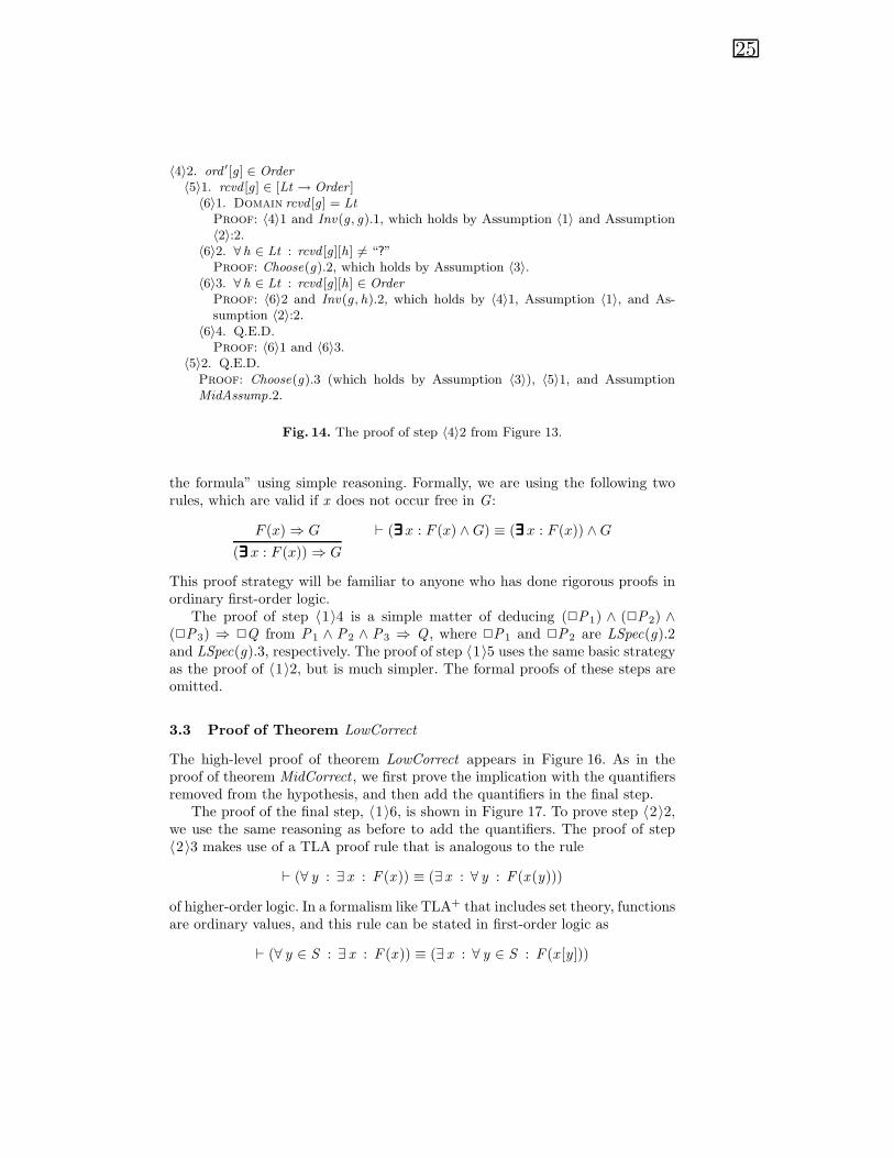
〈4〉2. ord ′[g ] ∈ Order〈5〉1. rcvd [g ] ∈ [Lt → Order ]〈6〉1. Domain rcvd [g ] = Lt

Proof: 〈4〉1 and Inv(g , g).1, which holds by Assumption 〈1〉 and Assumption〈2〉:2.

〈6〉2. ∀ h ∈ Lt : rcvd [g ][h] �= “?”Proof: Choose(g).2, which holds by Assumption 〈3〉.

〈6〉3. ∀ h ∈ Lt : rcvd [g ][h] ∈ OrderProof: 〈6〉2 and Inv(g , h).2, which holds by 〈4〉1, Assumption 〈1〉, and As-sumption 〈2〉:2.

〈6〉4. Q.E.D.Proof: 〈6〉1 and 〈6〉3.

〈5〉2. Q.E.D.Proof: Choose(g).3 (which holds by Assumption 〈3〉), 〈5〉1, and AssumptionMidAssump.2.

Fig. 14. The proof of step 〈4〉2 from Figure 13.

the formula” using simple reasoning. Formally, we are using the following tworules, which are valid if x does not occur free in G:

F (x) ⇒ G

(∃∃∃∃∃∃ x : F (x)) ⇒ G

� (∃∃∃∃∃∃x : F (x) ∧ G) ≡ (∃∃∃∃∃∃x : F (x)) ∧ G

This proof strategy will be familiar to anyone who has done rigorous proofs inordinary first-order logic.

The proof of step 〈1〉4 is a simple matter of deducing (✷P1) ∧ (✷P2) ∧(✷P3) ⇒ ✷Q from P1 ∧ P2 ∧ P3 ⇒ Q , where ✷P1 and ✷P2 are LSpec(g).2and LSpec(g).3, respectively. The proof of step 〈1〉5 uses the same basic strategyas the proof of 〈1〉2, but is much simpler. The formal proofs of these steps areomitted.

3.3 Proof of Theorem LowCorrect

The high-level proof of theorem LowCorrect appears in Figure 16. As in theproof of theorem MidCorrect , we first prove the implication with the quantifiersremoved from the hypothesis, and then add the quantifiers in the final step.

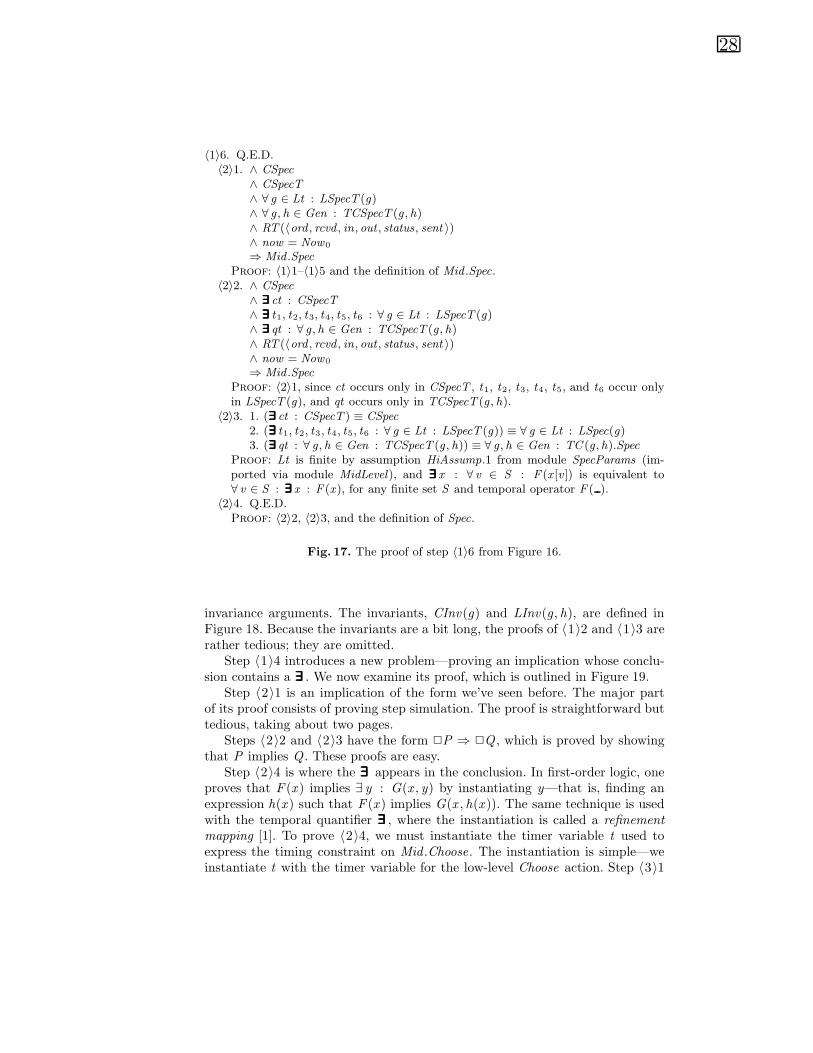
The proof of the final step, 〈1〉6, is shown in Figure 17. To prove step 〈2〉2,we use the same reasoning as before to add the quantifiers. The proof of step〈2〉3 makes use of a TLA proof rule that is analogous to the rule

� (∀ y : ∃ x : F (x )) ≡ (∃ x : ∀ y : F (x (y)))

of higher-order logic. In a formalism like TLA+ that includes set theory, functionsare ordinary values, and this rule can be stated in first-order logic as

� (∀ y ∈ S : ∃ x : F (x )) ≡ (∃ x : ∀ y ∈ S : F (x [y]))

26

〈1〉3. Assume: g ∈ LtProve: (now = Now0) ∧ RT (〈ord , rcvd , status 〉) ∧ LSpec(g)

∧ (∀ h ∈ Lt : ✷Inv(g , h))⇒ ✷TInv(g)

Let: LSpecT (g , t)∆= LSpec(g).1 ∧ LSpec(g).2 ∧ LSpec(g).3 ∧ LSpec(g).4(t)

TInvT (g , t)∆=

1.∧ now ∈ Real2.∧ Loyal(g) ∧ (ord [g ] = “?”) ∧ (∀ h ∈ Lt : rcvd [g ][h] �= “?”)

⇒ (now ≤ t ≤ Now0 + 2δ + ε)〈2〉1. (now = Now0) ∧ RT (〈ord , rcvd , status 〉) ∧ LSpecT (g , t)

∧ (∀ h ∈ Lt : ✷Inv(g , h))⇒ ✷TInvT (g , t). . .

〈2〉2. (now = Now0) ∧ RT (〈ord , rcvd , status 〉) ∧ LSpecT (g , t)∧ (∀ h ∈ Lt : ✷Inv(g , h))⇒ ✷TInv(g)

Proof: 〈2〉1 and simple temporal reasoning, since TInvT (g , t) implies TInv(g).〈2〉3. (∃∃∃∃∃∃ t : (now = Now0) ∧ RT (〈ord , rcvd , status 〉) ∧ LSpecT (g , t)

∧ (∀ h ∈ Lt : ✷Inv(g , h)))⇒ ✷TInv(g)Proof: 〈2〉2, since t does not occur free in ✷TInv(g).

〈2〉4. Q.E.D.Proof: 〈2〉3, since∃∃∃∃∃∃ t : ∧ (now = Now0) ∧ RT (〈ord , rcvd , status 〉)

∧ LSpecT (g , t)∧ ∀ h ∈ Lt : ✷Inv(g , h))

≡ {By definition of LSpecT .}∃∃∃∃∃∃ t : ∧ (now = Now0) ∧ RT (〈ord , rcvd , status 〉)

∧ LSpec(g).1 ∧ LSpec(g).2 ∧ LSpec(g).3 ∧ LSpec(g).4(t)∧ ∀ h ∈ Lt : ✷Inv(g , h)

≡ {Because t occurs free only in LSpecT (g).4.}∧ (now = Now0) ∧ RT (〈ord , rcvd , status 〉)∧ LSpec(g).1 ∧ LSpec(g).2 ∧ LSpec(g).3 ∧ ∃∃∃∃∃∃ t : LSpec(g).4(t)∧ ∀ h ∈ Lt : ✷Inv(g , h)

≡ {By definition of LSpec.}∧ (now = Now0) ∧ RT (〈ord , rcvd , status 〉)∧ LSpec(g)∧ ∀ h ∈ Lt : ✷Inv(g , h)

Fig. 15. The proof of 〈1〉3 from Figure 11, with the proof of 〈2〉1 elided.

27

Theorem Spec ⇒ Mid .Spec

Let: qt , ct , t1, t2, t3, t4, t5, t6 : variable

TEMax(t , g ,A)∆= VTimer(t ,A, ε, lvar(g)) ∧MaxTimer(t)

CSpecT∆= 1.∧ CInit ∧✷[CNext ]cvar

2.∧ ∀ g ∈ Lt : TEMax(ct [g ], Cmdr , CSend(g))

LSpecT (g)∆= 1.∧ LInit(g) ∧ ✷[LNext(g)]lvar(g)

2.∧ TEMax(t1[g ], g , Issue(g))3.∧ TEMax(t2[g ], g , IssueTimeout(g))4.∧ TEMax(t3[g ], g ,Choose(g))5.∧ ∀ h ∈ Lt \ {g} :

∧ TEMax(t4[g ][h], g ,Send(g , h))∧ TEMax(t5[g ][h], g ,Relay(g , h))∧ TEMax(t6[g ][h], g ,RelayTimeout(g , h))

TCSpecT (g , h)∆= TC (g , h).Spec.1 ∧ TC (g ,h).Spec.2

∧TC (g , h).Spec.3(qt [g ][h])

CInv(g)∆= . . .

LInv(g , h)∆= . . .

〈1〉1. CSpec ⇒ Mid .Hi .CSpec〈1〉2. Assume: g ∈ Lt

Prove: ∧ CSpecT ∧ LSpecT (g)∧ TCSpecT (Cmdr , g)∧ (now = Now0) ∧ RT (〈ord , rcvd , in, out , status, sent 〉)⇒ ✷CInv(g)

〈1〉3. Assume: 1. g , h ∈ Lt2. g �= h

Prove: ∧ LSpecT (g) ∧ LSpecT (h)∧ TCSpecT (g , h)∧ (now = Now0) ∧ RT (〈ord , rcvd , in, out , status, sent 〉)∧ ✷CInv(g)⇒ ✷LInv(g , h)

〈1〉4. Assume: g ∈ LtProve: LSpec(g) ∧ ✷CInv(g) ∧ ✷(∀ h ∈ Lt \ {g} : LInv(h, g))

⇒ Mid .LSpec(g)〈1〉5. RT (〈ord , rcvd , in, out , status 〉)⇒ RT (〈ord , rcvd , status 〉)〈1〉6. Q.E.D.

Fig. 16. The high-level proof of theorem LowCorrect.

(The range S is needed because the domain of a function must be a set.) If theordinary existential quantifier ∃ is replaced by the temporal quantifier ∃∃∃∃∃∃ , therule remains sound in general only if S is finite.4

We now return to the high-level proof of the theorem. The proof of step〈1〉1 is simple and is omitted. The proofs of 〈1〉2 and 〈1〉3 are straightforward

4 The rule is unsound for an infinite set S because ∃∃∃∃∃∃ is defined so ∃∃∃∃∃∃ x : F is invariantunder stuttering. It is sound for the operator ∃∃∃∃∃∃ of Manna and Pnueli [18], whichdoes not preserve invariance under stuttering.

28

〈1〉6. Q.E.D.〈2〉1. ∧ CSpec

∧ CSpecT∧ ∀ g ∈ Lt : LSpecT (g)∧ ∀ g , h ∈ Gen : TCSpecT (g , h)∧ RT (〈ord , rcvd , in,out , status, sent 〉)∧ now = Now0

⇒ Mid .SpecProof: 〈1〉1–〈1〉5 and the definition of Mid .Spec.

〈2〉2. ∧ CSpec∧ ∃∃∃∃∃∃ ct : CSpecT∧ ∃∃∃∃∃∃ t1, t2, t3, t4, t5, t6 : ∀ g ∈ Lt : LSpecT (g)∧ ∃∃∃∃∃∃ qt : ∀ g , h ∈ Gen : TCSpecT (g , h)∧ RT (〈ord , rcvd , in,out , status, sent 〉)∧ now = Now0

⇒ Mid .SpecProof: 〈2〉1, since ct occurs only in CSpecT , t1, t2, t3, t4, t5, and t6 occur onlyin LSpecT (g), and qt occurs only in TCSpecT (g , h).

〈2〉3. 1. (∃∃∃∃∃∃ ct : CSpecT ) ≡ CSpec2. (∃∃∃∃∃∃ t1, t2, t3, t4, t5, t6 : ∀ g ∈ Lt : LSpecT (g)) ≡ ∀ g ∈ Lt : LSpec(g)3. (∃∃∃∃∃∃ qt : ∀ g , h ∈ Gen : TCSpecT (g , h)) ≡ ∀ g , h ∈ Gen : TC (g ,h).Spec

Proof: Lt is finite by assumption HiAssump.1 from module SpecParams (im-ported via module MidLevel), and ∃∃∃∃∃∃ x : ∀ v ∈ S : F (x [v ]) is equivalent to∀ v ∈ S : ∃∃∃∃∃∃ x : F (x), for any finite set S and temporal operator F ( ).

〈2〉4. Q.E.D.Proof: 〈2〉2, 〈2〉3, and the definition of Spec.

Fig. 17. The proof of step 〈1〉6 from Figure 16.

invariance arguments. The invariants, CInv(g) and LInv(g, h), are defined inFigure 18. Because the invariants are a bit long, the proofs of 〈1〉2 and 〈1〉3 arerather tedious; they are omitted.

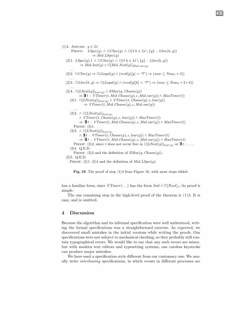
Step 〈1〉4 introduces a new problem—proving an implication whose conclu-sion contains a ∃∃∃∃∃∃ . We now examine its proof, which is outlined in Figure 19.

Step 〈2〉1 is an implication of the form we’ve seen before. The major partof its proof consists of proving step simulation. The proof is straightforward buttedious, taking about two pages.

Steps 〈2〉2 and 〈2〉3 have the form ✷P ⇒ ✷Q , which is proved by showingthat P implies Q . These proofs are easy.

Step 〈2〉4 is where the ∃∃∃∃∃∃ appears in the conclusion. In first-order logic, oneproves that F (x ) implies ∃ y : G(x , y) by instantiating y—that is, finding anexpression h(x ) such that F (x ) implies G(x , h(x )). The same technique is usedwith the temporal quantifier ∃∃∃∃∃∃ , where the instantiation is called a refinementmapping [1]. To prove 〈2〉4, we must instantiate the timer variable t used toexpress the timing constraint on Mid .Choose. The instantiation is simple—weinstantiate t with the timer variable for the low-level Choose action. Step 〈3〉1

29

Let: r(g , h)∆= if rcvd [g ][h] = “?” then 〈 〉

else 〈rcvd [g ][h]〉c(g , h)

∆= in[h][g ][1] ◦ out [g ][h][1]

cOrd(g)∆= r(g , g) ◦ c(Cmdr , g)

lOrd(g , h)∆= r(g , h) ◦ c(h, g)

CInv(g)∆=

1.∧ Loyal(Cmdr) ∧ Loyal(g)⇒∨ (cOrd(g) = 〈 〉) ∧NotSent(Cmdr , g)∨ (cOrd(g) = 〈ord [Cmdr ]〉) ∧ ¬NotSent(Cmdr , g)

2.∧ Loyal(g) ∧ (rcvd [g ][g ] = “?”)⇒ ∀ h ∈ Lt : NotSent(g , h)3.∧ Loyal(Cmdr) ∧ NotSent(Cmdr , g)⇒ (now ≤ ct [g ] ≤ Now0 + ε)4.∧ Loyal(g) ∧ Loyal(Cmdr) ∧ (out [Cmdr ][g ][1] �= 〈 〉)

⇒ (now ≤ qt [Cmdr ][g ] ≤ Now0 + τ + ε)5.∧ Loyal(g) ∧ Loyal(Cmdr) ∧ (in[g ][Cmdr ][1] �= 〈 〉)

⇒ (now ≤ t1[g ] ≤ Now0 + τ + 2 ∗ ε)6.∧ Loyal(g) ∧ (rcvd [g ][g ] = “?”) ∧ (Now0 + τ + 2 ∗ ε < now)

⇒ (now ≤ t2[g ] ≤ Now0 + τ + 3 ∗ ε)7.∧ now ∈ Real

LInv(g , h)∆=

1.∧ Loyal(g) ∧ Loyal(h)⇒ ∨ (lOrd(h, g) = 〈 〉) ∧ NotSent(g , h)∨ (lOrd(h, g) = 〈rcvd [g ][g ]〉) ∧ ¬NotSent(g , h)

2.∧ Loyal(g) ∧ (rcvd [g ][g ] �= “?”) ∧NotSent(g , h)⇒ (now ≤ t4[g ][h] ≤ Now0 + τ + 4 ∗ ε)

3.∧ Loyal(g) ∧ Loyal(h) ∧ (out [g ][h][1] �= 〈 〉)⇒ (now ≤ qt [g ][h] ≤ Now0 + 2 ∗ τ + 4 ∗ ε)

4.∧ Loyal(g) ∧ Loyal(h) ∧ (in[h][g ][1] �= 〈 〉)⇒ (now ≤ t5[h][g ] ≤ Now0 + 2 ∗ τ + 5 ∗ ε)

5.∧ Loyal(h) ∧ (rcvd [h][g ] = “?”) ∧ (now > Now0 + 2 ∗ τ + 5 ∗ ε)⇒ (now ≤ t6[h][g ] ≤ Now0 + 2 ∗ τ + 6 ∗ ε)

Fig. 18. The invariants for the proof of theorem LowCorrect.

30

〈1〉4. Assume: g ∈ LtProve: LSpec(g) ∧ ✷CInv(g) ∧ ✷(∀ h ∈ Lt \ {g} : LInv(h, g))

⇒ Mid .LSpec(g)

〈2〉1. LSpec(g).1 ∧ ✷CInv(g) ∧ ✷(∀ h ∈ Lt \ {g} : LInv(h, g))⇒ Mid .Init(g) ∧ ✷[Mid .Next(g)]Mid.var(g)

. . .〈2〉2. ✷CInv(g)⇒ ✷(Loyal(g) ∧ (rcvd [g ][g ] = “?”)⇒ (now ≤ Now0 + δ))

. . .〈2〉3. ✷LInv(h, g)⇒ ✷(Loyal(g) ∧ (rcvd [g ][h] = “?”)⇒ (now ≤ Now0 + 2 ∗ δ))

. . .〈2〉4. ✷[LNext(g)]lvar(g) ∧ EMax(g , Choose(g))

⇒ ∃∃∃∃∃∃ t : VTimer(t ,Mid .Choose(g), ε,Mid .var(g)) ∧MaxTimer(t)〈3〉1. ✷[LNext(g)]lvar(g) ∧VTimer(t , Choose(g), ε, lvar(g))

⇒ VTimer(t , Mid .Choose(g), ε,Mid .var(g)). . .

〈3〉2. ∧ ✷[LNext(g)]lvar(g)

∧ VTimer(t ,Choose(g), ε, lvar(g)) ∧MaxTimer(t)⇒ ∃∃∃∃∃∃ t : VTimer(t ,Mid .Choose(g), ε,Mid .var(g)) ∧MaxTimer(t)

Proof: 〈3〉1.〈3〉3. ∧ ✷[LNext(g)]lvar(g)

∧ ∃∃∃∃∃∃ t : VTimer(t ,Choose(g), ε, lvar(g)) ∧MaxTimer(t)⇒ ∃∃∃∃∃∃ t : VTimer(t ,Mid .Choose(g), ε,Mid .var(g)) ∧MaxTimer(t)

Proof: 〈3〉2, since t does not occur free in ✷[LNext(g)]lvar(g) or ∃∃∃∃∃∃ t : . . . .〈3〉4. Q.E.D.

Proof: 〈3〉2 and the definition of EMax(g ,Choose(g)).〈2〉5. Q.E.D.

Proof: 〈2〉1–〈2〉4 and the definition of Mid .LSpec(g).

Fig. 19. The proof of step 〈1〉4 from Figure 16, with most steps elided.

has a familiar form, since VTimer(. . .) has the form Init ∧✷[Next ]v ; its proof issimple.

The one remaining step in the high-level proof of the theorem is 〈1〉5. It iseasy, and is omitted.

4 Discussion

Because the algorithm and its informal specification were well understood, writ-ing the formal specifications was a straightforward exercise. As expected, wediscovered small mistakes in the initial versions while writing the proofs. Ourspecifications were not subject to mechanical checking, so they probably still con-tain typographical errors. We would like to say that any such errors are minor,but with modern text editors and typesetting systems, one careless keystrokecan produce major mistakes.

We have used a specification style different from our customary one. We usu-ally write interleaving specifications, in which events in different processes are

31

represented by separate steps [3]. Here, we have written noninterleaving spec-ifications that allow individual steps which represent actions in two or moreprocesses. For example, the formula Spec of module MidLevel allows behaviorsin which a single step is both an Issue(g) step of lieutenant g and a Relay(h, g)step of a different lieutenant h. Writing noninterleaving specifications introducedno new problems.

Writing the proofs was also a straightforward exercise. As is typical whenreasoning about real time, our specifications are safety properties; there are noliveness properties. When proving safety properties, creativity is required only infinding the invariants. With practice, writing invariants becomes second nature.The rest of the proof is a standard process of applying simple TLA proof rules andusing the structure of the formulas to decompose the resulting proof obligations.

Writing this kind of proof is an exercise in organizing a complex structure. Itis very much like programming; it is completely different from what mathemati-cians do when they write proofs. All the steps in our proof are mathematicallytrivial. Hierarchically structured proofs are long and tedious, but they are theonly kind of hand proofs that can be trusted. There are no shortcuts. Shortproofs are short because they gloss over details that have to be checked to avoiderrors.

These proofs are amenable to mechanical verification. Most steps can bechecked with the TLP verification system [7]. However, for this type of rea-soning, which cannot be checked by finite-state methods, mechanical theoremproving still seems to be considerably more work than writing a hand proof. Thehierarchical proof style makes it possible to reduce the probability of errors inhand proofs to an acceptable level.

Our specifications are written in TLA+. The flexibility of TLA+ is indicatedby the ease with which real-time properties are expressed, even though the lan-guage has no special primitives for time. We use the same RealTime module forspecifying Byzantine generals that was used in [15] for specifying a gas burner.This kind of flexibility and modularity are characteristic of an engineering dis-cipline.

Our proofs use the logic TLA. They are completely formal. Although mostof the lower-level steps were omitted, the parts that we did present in detailshow that all the proofs can be carried out to the level of simple propositionalreasoning. The proofs are seamless. The theorems to be proved are mathematicalformulas, and at each step we are proving a mathematical formula. There is noswitching from programs to logic; there is no appeal to semantic understanding.Hierarchically decomposing a large problem into smaller ones by the use of simplemathematical rules is characteristic of an engineering discipline.

We believe that formal specification and proof is now feasible for high-leveldesigns of real systems. They are not yet feasible for reasoning at the level ofexecutable code, except in special applications or for small parts of a system. Itmay appear that it is difficult to reason about code because our specificationsare logical formulas rather than programs. However, the primary issue is not oneof language but of complexity. It is hard to reason about real programs because

32

they are complicated. Formal reasoning is generally applied only to concurrentprograms written in toy languages like CSP [8] and Unity [5]. A program in atoy language is no closer to a real program than is a TLA formula. Further workis needed before formal reasoning about executable code becomes routine.

References

1. Martın Abadi and Leslie Lamport. The existence of refinement mappings. Theo-retical Computer Science, 82(2):253–284, May 1991.

2. Martın Abadi and Leslie Lamport. An old-fashioned recipe for real time. ResearchReport 91, Digital Equipment Corporation, Systems Research Center, 1992. Anearlier version, without proofs, appeared in [6, pages 1–27].

3. Martın Abadi and Leslie Lamport. Conjoining specifications. Research Report118, Digital Equipment Corporation, Systems Research Center, 1993. To appearin ACM Transactions on Programming Languages and Systems.

4. E. A. Ashcroft. Proving assertions about parallel programs. Journal of Computerand System Sciences, 10:110–135, February 1975.

5. K. Mani Chandy and Jayadev Misra. Parallel Program Design. Addison-Wesley,Reading, Massachusetts, 1988.

6. J. W. de Bakker, C. Huizing, W. P. de Roever, and G. Rozenberg, editors. Real-Time: Theory in Practice, volume 600 of Lecture Notes in Computer Science.Springer-Verlag, Berlin, 1992. Proceedings of a REX Real-Time Workshop, heldin The Netherlands in June, 1991.

7. Urban Engberg, Peter Grønning, and Leslie Lamport. Mechanical verification ofconcurrent systems with TLA. In Computer-Aided Verification, Lecture Notesin Computer Science, Berlin, Heidelberg, New York, June 1992. Springer-Verlag.Proceedings of the Fourth International Conference, CAV’92.

8. C. A. R. Hoare. Communicating Sequential Processes. Series in Computer Science.Prentice-Hall International, London, 1985.

9. Reino Kurki-Suonio. Operational specification with joint actions: Serializabledatabases. Distributed Computing, 6(1):19–37, 1992.

10. Simon S. Lam and A. Udaya Shankar. Protocol verification via projections. IEEETransactions on Software Engineering, SE-10(4):325–342, July 1984.

11. Simon S. Lam and A. Udaya Shankar. Specifying modules to satisfy interfaces: Astate transition system approach. Distributed Computing, 6(1):39–63, 1992.

12. Leslie Lamport. Specifying concurrent program modules. ACM Transactions onProgramming Languages and Systems, 5(2):190–222, April 1983.

13. Leslie Lamport. The temporal logic of actions. Research Report 79, Digital Equip-ment Corporation, Systems Research Center, December 1991. To appear in ACMTransactions on Programming Languages and Systems.

14. Leslie Lamport. How to write a proof. Research Report 94, Digital EquipmentCorporation, Systems Research Center, February 1993. To appear in AmericanMathematical Monthly.

15. Leslie Lamport. Hybrid systems in TLA+. In Robert L. Grossman, Anil Nerode,Anders P. Ravn, and Hans Rischel, editors, Hybrid Systems, volume 736 of Lec-ture Notes in Computer Science, pages 77–102, Berlin, Heidelberg, 1993. Springer-Verlag.

33

16. Leslie Lamport, Robert Shostak, and Marshall Pease. The Byzantine generalsproblem. ACM Transactions on Programming Languages and Systems, 4(3):382–401, July 1982.

17. Nancy Lynch and Mark Tuttle. Hierarchical correctness proofs for distributedalgorithms. In Proceedings of the Sixth Symposium on the Principles of DistributedComputing, pages 137–151. ACM, August 1987.

18. Zohar Manna and Amir Pnueli. The Temporal Logic of Reactive and ConcurrentSystems. Springer-Verlag, New York, 1991.

19. Jayadev Misra and K. Mani Chandy. Proofs of networks of processes. IEEE Trans-actions on Software Engineering, SE-7(4):417–426, July 1981.

20. Peter G. Neumann and Leslie Lamport. Highly dependable distributed systems.Technical report, SRI International, June 1983. Contract Number DAEA18-81-G-0062, SRI Project 4180.

34

module FiniteSets 3

import Naturals

HasCardinality(n,S)∆= let Q

∆= {i ∈ Nat : i < n}

in ∧ n ∈ Nat∧ ∃ f ∈ [Q → S ] :

∧ ∀ s ∈ S : ∃ q ∈ Q : f [q ] = s∧ ∀ q1, q2 ∈ Q : (f [q1] = f [q2])⇒ (q1 = q2)

IsFiniteSet(S)∆= ∃ n ∈ Nat : HasCardinality(n, S)

module Sequences 42

import Naturals

OneTo(n)∆= {i ∈ Nat : (1 ≤ i) ∧ (i ≤ n)}

Len(s)∆= choose n : (n ∈ Nat) ∧ (Domain s) = OneTo(n)

Head(s)∆= s[1]

Tail(s)∆= [i ∈ OneTo(Len(s) − 1) �→ s[i + 1]]

(s) ◦ (t) ∆= [i ∈ OneTo(Len(s) + Len(t)) �→ if i ≤ Len(s) then s[i ]

else t [i − Len(s)]]

module RealTime

import Reals

parameters now : variable∞ : constant

assumption

InfinityUnReal∆= ∞ /∈ Real

RT (v) 24 ∆= ∧ now ∈ Real∧ ✷[∧ now ′ ∈ {r ∈ Real : now < r}

∧ v ′ = v ]now

VTimer(x ,A, δ, v)∆= ∧ x = if Enabled 〈A〉v then now + δ

else ∞∧ ✷[x ′ = if (Enabled 〈A〉v )′

then if 〈A〉v ∨ ¬Enabled 〈A〉v then now ′ + δelse x

else ∞ ]〈x ,v 〉MaxTimer(x)

∆= ✷[(x �=∞)⇒ (now ′ ≤ x)]now

MinTimer(x ,A, v)∆= ✷[A⇒ (now ≥ x)]v

Fig. 20. The modules FiniteSets, Sequences, and RealTime.

35

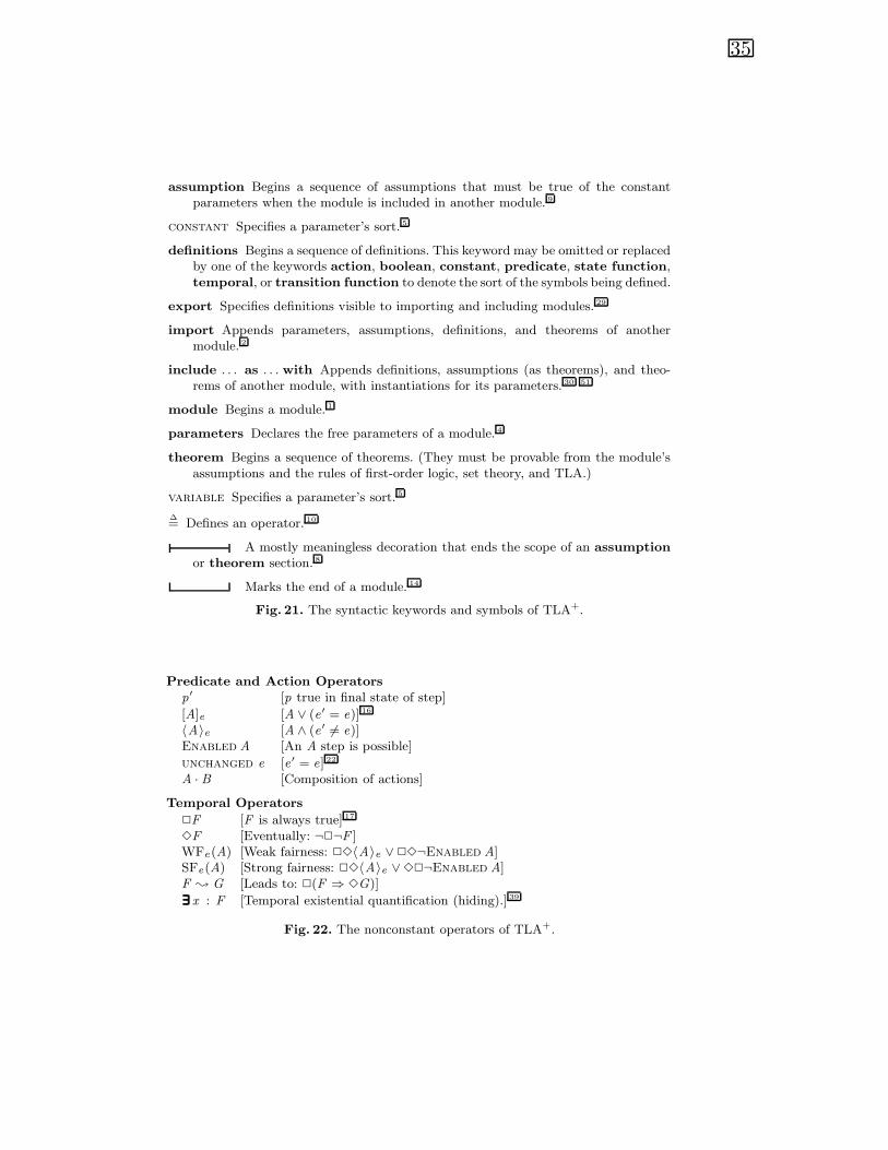
assumption Begins a sequence of assumptions that must be true of the constantparameters when the module is included in another module. 9

constant Specifies a parameter’s sort. 5

definitions Begins a sequence of definitions. This keyword may be omitted or replacedby one of the keywords action, boolean, constant, predicate, state function,temporal, or transition function to denote the sort of the symbols being defined.

export Specifies definitions visible to importing and including modules. 29

import Appends parameters, assumptions, definitions, and theorems of anothermodule. 2

include . . . as . . . with Appends definitions, assumptions (as theorems), and theo-rems of another module, with instantiations for its parameters. 30 51

module Begins a module. 1

parameters Declares the free parameters of a module. 4

theorem Begins a sequence of theorems. (They must be provable from the module’sassumptions and the rules of first-order logic, set theory, and TLA.)

variable Specifies a parameter’s sort. 5

∆= Defines an operator. 10

A mostly meaningless decoration that ends the scope of an assumptionor theorem section. 8

Marks the end of a module. 14

Fig. 21. The syntactic keywords and symbols of TLA+.

Predicate and Action Operatorsp′ [p true in final state of step]

[A]e [A ∨ (e ′ = e)] 16

〈A〉e [A ∧ (e ′ �= e)]Enabled A [An A step is possible]

unchanged e [e ′ = e] 22

A · B [Composition of actions]

Temporal Operators

✷F [F is always true] 17

✸F [Eventually: ¬✷¬F ]WFe(A) [Weak fairness: ✷✸〈A〉e ∨✷✸¬Enabled A]SFe(A) [Strong fairness: ✷✸〈A〉e ∨✸✷¬Enabled A]F ❀ G [Leads to: ✷(F ⇒ ✸G)]∃∃∃∃∃∃ x : F [Temporal existential quantification (hiding).] 39

Fig. 22. The nonconstant operators of TLA+.

36

Logictrue false ∧ ∨ ¬ ⇒ ≡∀ x : p ∃ x : p ∀ x ∈ S : p ∃ x ∈ S : pchoose x : p [Equals some x satisfying p]

Sets= �= ∈ /∈ ∪ ∩ ⊆ \ [set difference]{e1, . . . , en} [Set consisting of elements ei ]{x ∈ S : p} [Set of elements x in S satisfying p]{e : x ∈ S} [Set of elements e such that x in S ]Subset S [Set of subsets of S ]union S [Union of all elements of S ]

Functions

f [e] [Function application] 13

Domain f [Domain of function f ]

[x ∈ S �→ e] [Function f such that f [x ] = e for x ∈ S ] 32

[S → T ] [Set of functions f with f [x ] ∈ T for x ∈ S ] 28

[f except ![e1] = e2] [Function f equal to f except f [e1] = e2]34

[f except ![e] ∈ S ] [Set of functions f equal to f except f [e] ∈ S ]

Recordse.x [The x -component of record e][x1 �→ e1, . . . , xn �→ en ] [The record whose x i component is ei ][x1 : S1, . . . , xn : Sn ] [Set of all records with x i component in S i ][r except !.x = e] [Record r equal to r except r .x = e][r except !.x ∈ S ] [Set of records r equal to r except r .x ∈ S ]

Tuples

e[i ] [The i th component of tuple e]

〈e1, . . . , en 〉 [The n-tuple whose i th component is ei ]42

S1 × . . .× Sn [The set of all n-tuples with i th component in S i ]

Miscellaneous

“c1 . . . cn” [A literal string of n characters] 7

if p then e1 else e2 [Equals e1 if p true, else e2]case p1 → e1, . . . , pn → en [Equals ei if pi true]

let x1∆= e1 . . . xn

∆= en in e [Equals e in the context of the definitions]

∧ p1

. . .∧ pn

[the conjunction p1 ∧ . . . ∧ pn ] ∨ p1

. . .∨ pn

[the disjunction p1 ∨ . . . ∨ pn ]12

Fig. 23. The constant operators of TLA+.