SPECIFIC HEATS AT LOW TEMPERATURES

THE INTERNATIONAL CRYOGENICS MONOGRAPH SERIES

General Editors

Dr. K. Mendelssohn, F. R. S. The Clarendon Laboratory

Oxford, England

H. J. Goldsmid G. T. Meaden E. S. R. Gopal

Dr. K. D. Timmerhaus University of Colorado Boulder, Colorado

Thermoelectric Refrigeration, 1964 Electrical Resistance of Metals, 1965 Specific Heats at Low Temperatures, 1

Volumes in preparation

D. H. Parkinson and B. Mulhall J. L. Olsen and S. Gygax

A. J. Croft and P. V. E. McClintock G. K. Gaule

M. G. Zabetakis F. B. Canfield

W. E. Keller S. Ramaseshan

P. Glaser and A. Wechsler

Very High Magnetic Fields Superconductivity for Engineers Cryogenic Laboratory Equipment Superconductivity in Elements,

Alloys, and Compounds Cryogenic Safety Low-Temperature Phase Equilibria Helium-3 and Helium-4 Low-Temperature Crystallography Cryogenic Insulation Systems

SPECIFIC HEATS AT LOW TEMPERATURES

E. S. R. Gopal Department at Physics, Indian Institute at Science

Bangalore, India

ALBERT EMANUEL LIBRARY UNIVERSITY OF DAYTON

PLENUM PRESS NEW YORK

1966

ISBN 978-1-4684-9083-1 ISBN 978-1-4684-9081-7 (eBook) DOI 10.1007/978-1-4684-9081-7

Library of Congress Catalog Card Number 65-11339

© 1966 Plenum Press

Softcover reprint ofthe hardcover 1st edition 1966

A Division 01 Consultants Bureau Enterprises, [ne. 227 W. 17th St., N ew York, N. Y. 10011

All rights reserved

Preface

This work was begun quite some time ago at the University of Oxford during the tenure of an Overseas Scholarship of the Royal Commission for the Exhibition of 1851 and was completed at Banga­lore when the author was being supported by a maintenance allowance from the CSIR Pool for unemployed scientists. It is hoped that significant developments taking place as late as the beginning of 1965 have been incorporated.

The initial impetus and inspiration for the work came from Dr. K. Mendelssohn. To him and to Drs. R. W. Hill and N. E. Phillips, who went through the whole of the text, the author is obliged in more ways than one. For permission to use figures and other materials, grateful thanks are tendered to the concerned workers and institutions.

The author is not so sanguine as to imagine that all technical and literary flaws have been weeded out. If others come across them, they may be charitably brought to the author's notice as proof that physics has become too vast to be comprehended by a single onlooker.

Department of Physics Indian Institute of Science Bangalore 12, India November 1965

v

E. S. RAJA GoPAL

Contents

Introduction ................................................................. .

Chapter I Elementary Concepts of Specific Heats 1.1. Definitions.......................................... 5 1.2. Thermodynamics of Simple Systems............ 6 1.3. Difference Between Cp and Cv " •••••••.•••••••• 7 1.4. Variation of Specific Heats with

Temperature and Pressure.................. 10 1.5. Statistical Calculation of

Specific Heats................................. 11 1.6. Different Modes of Thermal Energy......... 12 1.7. Calorimetry .......................................... 16

Chapter 2 Lattice Heat Capacity 2.1. Dulong and Petit's Law ........................ 20 2.2. Equipartition Law .............................. 21 2.3. Quantum Theory of Specific Heats ......... 22 2.4. Einstein's Model ................................. 25 2.5. Debye's Model.................................... 28 2.6. Comparison of Debye's Theory

with Experiments.. ...... ...... ... .......... 31 2.7. Shortcomings of the Debye Model........... 35 2.8. The Born-Von Karman Model ............... 36 2.9. Calculation of g(v) ... ........... ...... .......... 40

2.10. Comparison of Lattice Theory with Experiments........................... 43

2.11. Debye () in Other Properties of Solids ...... 47

2.11.1. 0-Values from Elastic Properties. . . . . . . . . . . . 49 2.11.2. 0-Values from Compressibility and Melting

Point .................................. 50 2.11.3. O-Values from Thermal Expansion.. . . . . . . . . 50 2.11.4. 0-Values from Infrared Data .............. 51 2.11.5. O-Values from Electrical Resistivity.......... 52 2.11.6. Scattering of X-Rays, }'-Rays, and Neutrons.. 52

vii

viii

Chapter 3

Contents

Electronic Specific Heat 3.1. Specific Heat of Metals... ..... ................... 55 3.2. Quantum Statistics of an Electron

Gas............................................. 56 3.3. Specific Heat of Electrons in

Metals.......................................... 58 3.4. Electronic Specific Heat at Low

Temperatures. .... ...... ...................... 61 3.5. Specific Heat and Band Structure

of Metals . . . . . .. . ... . . . .. . . . . . . . .. . .. . . . . .. . . 64 3.6. Specific Heat of Alloys ..... ................... 68 3.7. Specific Heat of Semiconductors ............ 72 3.8. Phenomenon of Superconductivity......... 74 3.9. Specific Heat of Superconductors............ 76

3.10. Recent Studies ............................... ..... 80

Chapter 4 Magnetic Contribution to Specific Heats 4.1. Thermodynamics of Magnetic

Materials ... ....... .......................... 84 4.2. Types of Magnetic Behavior .................. 86 4.3. Spin Waves-Magnons ........................ 87 4.4. Spin Wave Specific Heats ..................... 89 4.5. The Weiss Model for Magnetic

Ordering.................................. ..... 93 4.6. The Heisenberg and Ising Models............ 95 4.7. Specific Heats Near the

Transition Temperature .................. 98 4.8. Paramagnetic Relaxation............ ........ .... 100 4.9. Schottky Effect... ................................. 102

4.10. Specific Heat of Paramagnetic Salts......... 105 4.11. Nuclear Schottky Effects........................ 109

Chapter 5 Heat Capacity of Liquids 5.1. Nature of the Liquid State . ................ .... 112 5.2. Specific Heat of Ordinary Liquids

and Liquid Mixtures ........................ 113 5.3. Liquid 4He at Low Temperatures ............ 114 5.4. Phonon and Roton Specific Heats ............ 116 5.5. Transition in Liquid 4He ........................ 120

Contents

Chapter 6

Chapter 7

Chapter 8

ix

5.6. Specific Heat of Liquid 3He..................... 123 5.7. Liquid 3He as a Fermi Liquid .................. 127 5.8. Mixtures of 4He and 3He ....... ................. 129 5.9. Supercooled Liquids-Glasses .................. 129

Specific Heats of Gases 6.1. Cp and Cv of a Gas .............................. 135 6.2. Classical Theory of Cv of Gases ............ 136 6.3. Quantum Theory of Cv of Gases .. .......... 138 6.4. Rotational Partition Function ............... 140 6.5. Homonuclear Molecules-Isotopes

of Hydrogen................................. 142 6.6. Vibrational and Electronic

Specific Heats .............................. 147 6.7. Calorimetric and Statistical Entropies

-Disorder in Solid State ............... 148 6.8. Hindered Rotation ................. ......... .... 152 6.9. Entropy of Hydrogen .... ....... ........... ..... 154

Specific-Heat Anomalies 7.1. Spurious and Genuine Anomalies............ 158 7.2. Cooperative and Noncooperative

Anomalies............. . ........ ............. . 161 7.3. Order-Disorder Transitions .................. 163 7.4. Onset of Molecular Rotation .................. 166 7.5. Ferroelectricity .................................... 167 7.6. Transitions in Rare-Earth Metals............ 170 7.7. Liquid-Gas Critical Points ................ ..... 175 7.8. Models of Cooperative Transitions 177

Miscellaneous Problems in Specific Heats 8.1. Specific Heat Near Phase Transitions 181 8.2. Specific Heat at Saturated

Vapor Pressure.............................. 185 8.3. Relaxation of Rotational and

Vibrational Specific Heats............... 186 8.4. Defects in Solids ..... ... .... ..... ................ 187 8.5. Surface Effects .................................... 190 8.6. Compilations of Specific-Heat Data ......... 192 8.7. Tabulations of Specific-Heat

Functions .................................... 194

x

Appendix (Six-Figure Tables of Einstein and Debye Internal-Energy and Specific-Heat Functions)

Contents

197

Author Index............................................................... 227

Subject Index............................................................... 234

Introduction

Investigations at temperatures below room temperature have advanced our knowledge in many ways. Toward the beginning of the present century, physical chemists evolved their reference state for chemical equilibria and thermodynamic properties on the basis of such studies. Later, physicists realized that a clear manifestation of quantum effects was possible at low temperatures. In recent times, superconductors, rocket fuels, cryopumping and a multitude of other developments have lifted low-temperature studies out of academic cloisters and into the realm of technology.

In any practical attempt to study low-temperature phenomena, the question of specific heats crops up immediately, in connection with the refrigeration needed to take care of the thermal capacity of the apparatus. Apart from its significance in this perennial problem of cooling equipments to desired low temperatures, knowledge of specific heats forms a powerful tool in many other areas, such as lattice vibrations, electronic distributions, energy levels in magnetic materials, and order-disorder phenomena in molecules. No better evidence for the usefulness of specific-heat studies is needed than the presence of the Debye characteristic temperature (j in so many branches of solid state studies. This monograph is basically a des­criptive introduction to the different aspects of specific-heat studies.

Historically, the need for measuring specific heats at low tempera­tures arose in conjunction with the formulation of the third law of thermodynamics. Nernst realized that the specific heat of all sub­stances should vanish as the absolute zero of temperature is approached. Einstein demonstrated the quantum effects that come into play in specific heats at low temperatures. This opened up the prospect of checking the energy states of all substances with the help of calorimetric measurements. Whatever theory of solid, liquid, and gaseous states is developed, it leads in the first place to a set of energy levels which the particles can occupy. By using suitable statistical methods, it is possible to compute the mean energy of the system and from it the specific heat Any such calculation requires a minimum of extra theoretical assumptions. This is both a strength

2 Introduction

and a weakness of specific-heat studies. The heat capacity provides a direct and immediate test of the theoretical model of the system, but because it is a measure of a mean quantity it cannot shed light on the finer details of the model. It is wise not to lose sight of this limitation-which, incidentally, holds true to some extent for the study of any phenomenological property of substances.

The reduction of specific heats at low temperatures is of tremen­dous significance in the practice of cryogenic techniques. For the ordinary materials used in the construction of apparatus, the specific heat is about 6 cal/gram-atom'degK at room temperature (300 OK), approximately 4 units at liquid-air temperature (80 OK), and only 10- 2 units at liquid-helium temperature (4 OK). The rapid fall in specific heats in the liquid hydrogen-helium temperature range makes itself felt in several ways. Once a large apparatus has been cooled to liquid-air temperature, relatively small amounts of refrigera­tion (measured in terms of, say, the latent heat of the liquid helium that is boiled away) are sufficient to cool it to about 4°K. It is, in fact, a standard practice to conserve liquid helium by precooling the cryostats with liquid air, and if possible liquid hydrogen, so that little helium is boiled away in reducing the temperature to the vicinity of 4 oK. Secondly, if a part of the cold apparatus is thermally insulated from the main heat sink, its temperature may rise considerably because of small amounts of heat influx. Such situations commonly arise in the measurement of specific heats. For the same reason, when very low temperatures « 1 OK) are achieved by adiabatic demagnetization, it is of utmost importance to cut out as much stray heat input as possible. Thirdly, because of the small heat capacity at low temperatures, thermal equilibrium among the various parts of an apparatus is established very quickly. Typically, a system which takes about an hour to come to internal equilibrium at room temperature will do so in about a minute at 4 oK.

It was mentioned above that the energy levels of the particles specify the mean energy of the system, which in turn determines the specific heat of the system. These energy levels may be in the form of translational, rotational, or vibrational motions of molecules in gases, vibrations of atoms about their lattice sites in solids, the wandering of electrons free to move in metals, and so on. The enumeration of the possible modes of energy can be continued further, and it is obvious that a discussion of the specific heats of substances must inevitably cover a very wide field, since any temperature-dependent phenomenon can contribute to specific heats. In a monograph such as this, it is both unnecessary and impossible to be comprehensive in the description of all phenomena which bear some slight relationship to specific heats. The solution attempted here is to provide a reasonably

Introduction 3

comprehensive description of the various aspects of specific-heat studies at low temperatures, leaving the discussion of allied pheno­mena to various other texts. 1 It has been a difficult task to steer between the Scylla of encyclopedic completeness and the Charybdis of shallow banality.

This compromise has been chosen to serve two purposes. For the interested neophyte, the monograph should be a simple survey and a stepping-stone to an understanding of the problems of specific heats. Thus, in discussing the basic principles, no attempt at rigor is made. In citing references, preference is given, if possible, to elemen­tary texts rather than to advanced treatises. If in this process several authors feel themselves overlooked, it is because the choice is not meant to be a judgment of the scientific value of such works, but is only a didactic device for elucidating the basic questions. Further, the normal behavior of solids, liquids, and gases is treated first before taking up, in Chapter 7, abnormalities in the specific heat of some substances. No doubt, the reader will find that some instances of specific-heat anomalies are introduced surreptitiously in Chapters 3 to 6, but the present arrangement has the added advantage that by Chapter 7 enough anomalies have been mentioned to focus attention on classification of such behavior. For those actively engaged with cryogenic problems, a description of the many facets of specific-heat studies, with adequate references to the sources of more detailed analyses of any single aspect, should make the book useful.

The task of listing all the references, especially to the early literature on the subject, has been rendered superfluous by the monu­mental work of Partington.2 Therefore, references to early papers are seldom given, and anyone interested can trace such papers from either the above treatise2 or the recent reviews and books cited at the end of each chapter. Moreover, the description of cryogenic tech­niques has been limited to a minimum because of the availability of excellent books on the subject. 3

REFERENCES I. C. F. Squire, Low Temperature Physics, McGraw-Hill, New York, 1953. K.

Mendelssohn, Cryophysics, Interscience, New York, 1960. L. C. Jackson, Low Tem­perature Physics, Methuen, London, 1962. R. W. Vance and W. M. Duke, Applied Cryogenic Engineering, Wiley, New York, 1962. H. M. Rosenberg, Low Tempera­ture Solid State Physics, Clarendon, Oxford, 1963. M. McClintock, Cryogenics, Reinhold, New York, 1964.

2. J. R. Partington, Advanced Treatise on Physical Chemistry, Longmans-Green, London; Vol. I, Properties of Gases (1949); Vol. II, Properties of Liquids (195\); Vol. Ill, Properties of Solids (1952).

4 Introduction

3. G. K. White, Experimental Techniques in Low Temperature Physics, Clarendon, Oxford, 1959. R. B. Scott, Cryogenic Engineering, Van Nostrand, New York, 1959. F. Din and A. H. Cockett, Low Temperature Techniques, Newnes, London, 1960. F. E. Hoare, L. C. Jackson, and N. Kurti, Experimental Cryophysics, Butterworth, London, 1961. A. C. Rose-Innes, Low Temperature Techniques, English University Press, London, 1964.

Chapter 1

Elementary Concepts of Specific Heats

1.1. DEFINITIONS

The specific heat of a substance is defined as the quantity of heat required to raise the temperature of a unit mass of the substance by a unit degree of temperature. To some extent, the specific heat depends upon the temperature at which it is measured and upon the changes that are allowed to take place during the rise of temperature. If the properties x, y, ... , are held constant when a heat input dQ raises the temperature of unit mass of the substance by dT, then

c , = lim (dQ) x.}.... dT dT~O x.y ....

(1.1)

The specific heat, sometimes called the heat capacity, is in general a positive quantity. In the absence of any rigid convention, it seems best to use the term specific heat when referring to 1 g of the material and the term heat capacity when a more general amount of the material, i.e., a gram-atom or a gram-molecule, is involved.

In expressing the numerical values of specific heats, the MKS system, based on kilogram units of the substance, is not yet widely used in current literature, and so cgs units will be used throughout the book. By convention, cx •y .... refers to the specific heat per gram and ex.}, ... to the heat capacity per gram-molecule of the substance. The Cx ... value is usually expressed in caljg·degK or in J/g'deg, the present conversion factor being 1 thermochemical calorie = 4.1840 J. In engineering literature, it is still not uncommon to find specific heats in BTU /lb'degF, which luckily has almost the same value in caljg·degK.

5

6 Chapter I

1.2. THERMODYNAMICS OF SIMPLE SYSTEMS

All processes in which quantities of heat and work come into play are governed by the fundamental laws of thermodynamics. Some properties of specific heats follow immediately from these laws, and it is therefore appropriate to consider them first. A dis­cussion of the principles of thermodynamics is given in several well­known texts.! If a quantity of heat dQ is supplied to a substance, a part of it goes to increase the internal energy E of the system and a part is utilized in performing external work W In accordance with the first law,

dQ = dE + dW (1.2)

If the heat exchange is reversible, the second law of thermodynamics permits calculation of the entropy S of the system from the relation

dQ = T dS (1.3)

Apart from the special conditions to be discussed in Section 8.5, E and S are proportional to the mass of the substance; that is, they are extensive variables.

It is instructive to start with a simple substance, namely, the ideal fluid. In gases and liquids, the pressure P at a point is the same in all directions, and any work done by the system dW is an expansion against the pressure. Then dW must be of the form

dW = PdV (1.4)

Moreover, fluids obey an equation of state

f(P, V, T) = 0 (1.5)

This means that anyone of P, V, T can be expressed in terms of the other two and that only two of the three quantities can be arbitrarily varied at the same time. Hence, during the change of temperature, either P or V can be kept constant, and correspondingly there are two principal heat capacities:

Cp = (:~)p = T(:~)p

Cv = (:~l = T(:~)v (1.6)

The case for solids is somewhat more complicated. Unlike ordinary fluids, which require forces only for changing their volume, solids require forces both to change their linear dimensions and to alter their shape. It is shown in the texts on elasticity2 that dW is of

Elementary Concepts of Specific Heats

the form

dW= Itjdej j

7

(i = 1,2, ... ,6)

where tj are the stresses and ej are the strains. Obviously, it is possible in principle to define a large number of specific heats, allowing only one stress or strain component to change during the heating. In practice, however, such experiments are hardly feasible, and only Cp , Cv are of importance. It can be shown3 that they obey the same thermodynamic relations as the C P' CV of liquids and gases, so there is no significant loss of generality in restricting the discussion to the simple case of fluids.

Combining (1.2) and 0.3), one can write the change in internal energy as

dE = TdS - PdV (1.7)

Often it is convenient to handle the other principal thermodynamic functions of the system, namely, enthalpy H, Helmholtz function A and Gibbs' function G, whose variations are

dH = d(E + P V) = T dS + V dP

dA = d(E - TS) = - S dT - P dV

dG = d(E - TS + PV) = - S dT + V dP

(1.8)

(1.9)

(1.10)

These four functions are nothing but measures of the energy content of the substance under various conditions, and the changes in these must depend only upon the initial and final states. Mathematically equivalent is the statement that the differentials (1.7) to (1.10) are perfect differentials; this condition leads to the four Maxwell's relations

(1.11)

The four relations are useful in expressing thermodynamic formulas in terms of quantities which are experimentally measured.

1.3. DIFFERENCE BETWEEN Cp and Cv

As an illustration of the use of equation (1.11), the important expressions for Cp - Cv may be calculated. Take T and V as the independent variables in describing the entropy of a mole of substance

8 Chapter I

and write

or

Replacing (ClS/ClVh by (ClP/ClT)v and using equations (1.6) yields

C p - C v = T(:~)p - T(:~)v = T(!~)J:~)p (1.12)

This relation is convenient if the equation of state is known explicitly. For example, a mole of a gas obeys the relation PV = RT under ideal conditions, and so equation (1.12) gives the difference between the molar heat capacities:

C p - C v = R (1.13)

The gas constant R has a value 8·314 J/mole'deg, or 1.987 caljmole·deg. For liquids and solids, (ClP/ClT)v is not easy to measure and is best eliminated from the equations. To do this, consider P as a function of Tand V:

dP = G~)T dV + G~), dT

At constant pressure, dP = 0, and

Now the coefficient of cubical expansion [3 = V-1(ClV/ClT)p and the isothermal compressibility kT = - V-1(ClV/ClPh are amenable to experimental measurements. In terms of [3, kT , and the molar volume V,

TV[32 C p - C v =-,;:;- (1.14)

The mechanical stability of a substance requires kT > O. There­fore, C p is always greater than C v' They are equal when [3 = 0, as in the case of water near 4°e, liquid 4He near 1.1 oK, and liquid 3He near 0.6°K. The reason for C p ~ C v is easy to see. Heating the sub­stance at constant pressure causes an increase in the internal energy

Elementary Concepts of Specific Heats 9

and also forces the substance to do external work in expanding against the pressure of the system. On the other hand, in heating at constant volume there is no work done against the pressure and all the heat goes to raise the internal energy. Hence, in the latter case the tempera­ture rise is larger for a given dQ. In other words, C v is less than C p.

The difference between C p and C v is about 5 % in most solids at room temperature. It decreases rapidly as the temperature is lowered. Table 1.1 gives the values for copper, and the behavior of other solids is very similar. However, to calculate C p - C v exactly, a tremendous amount of data is needed. The complete temperature dependence of molar volume, volume expansion, and isothermal compressibility, besides C P' should be known, and this knowledge is not always available. Under such conditions, approximate relations are used. The most successful one is the Nernst-Lindemann relation based on Grtineisen's equation of state:

(1.15)

The parameter A is nearly constant over a wide range of temperature. For example, in copper A = 1.54 X 10- 5 mole/cal at 10000K and 1.53 x 10- 5 at 100oK, if the mechanical equivalent of heat is taken as 4.184 x 107 ergs/cal. If A is calculated at anyone temperature from the values of V, p, and kT' it may be used to calculate C p - Cv over a wide range of T without serious error.

In gases at low pressures, C p - Cv is equal to R [equation (1.13)], but at high pressures small corrections for nonideality are needed. 1

The values of Cp or Cv are not dramatically changed at low tempera­tures. The behavior of nitrogen is typical: Cp is about 6.95 caIjmole.deg at 300 0 K and about 6.96 at 100 OK.

The ratio of specific heats C JCv is nearly unity for solids and liquids, but not for gases. The value C p '" 1R for nitrogen shows that Cv '" iR, and so CJCv '" 1.4. It is 1.67 for monatomic gases such as helium or argon, and becomes approximately 1.3 for polyatomic

Table 1.1. Cp and Cv for Copper

T c p V P kT c p - c. c. cp/c.

1000 7.04 7.35 65.2 0.976 0.778 6.27 1.12 300 5.87 7.06 49.2 0.776 0.157 5.71 1.03 100 3.88 7.01 31.5 0.721 0.023 3.86 1.00

4 0.0015 7.00 0.0 0.710 0.0 0.0015 1.00

Tin degK; cp , C. in caljmole·deg; Yin cm3/mole; pin W- 6/deg; kT in 10- 12 cm 2/dyne.

10 Chapter 1

gases. In general, the ratio C riC v depends upon the state of the sub­stance and is useful in converting adiabatic elastic data to isothermal data. For example, it is a simple exercise to show that

kT Cp

ks Cv 0.16)

where kT is the isothermal compressibility and ks is the adiabatic value. The ratio has greater significance for gases, where, besides being involved in the adiabatic equation PVcp/cv = constant, it also gives information about the number of degrees of freedom of the molecules constituting the gas.

1.4. V ARIA nON OF SPECIFIC HEATS WITH TEMPERATURE AND PRESSURE

It was mentioned in Section 1.1 that the specific heats depend to some extent upon the state of the substance, and Table 1.1 shows how C p' C v in a solid are affected by temperature. The full details of such temperature dependences are very complicated, and their elucidation is the major task of the whole book. Here, only some simple consequences of general thermodynamic considerations are pointed out.

The use of Maxwell's relations (1.11) shows that

(~~)T = T(!~)v (aa~ \ = - TG~)p (1.17)

The prime use of these relations is in reducing the measured specific heats of gases to the ideal values at zero pressure with the help of the equation of state. For a perfect gas, C p and Cv are independent of pressure.

The third law of thermodynamics specifies the behavior of specific heats at very low temperature. According to it, the entropy of any system in thermodynamic equilibrium tends to zero at the absolute zero. Since S = 0 at T = 0 and S is finite at higher temperatures, the difference in entropy at constant volume between T = 0 and T = To may be obtained from equation (1.6) as

Elementary Concepts of Specific Heats 11

For the integral to converge, i.e., remain finite definite, at the lower limit T = 0, Cv/T must be a finite number (including zero) as T ..... O. In other words, when absolute zero is approached, the specific heat must tend to zero at least as the first power of T.

The vanishing of specific heats at T = 0 is of great importance because it permits the use ofooK as a reference for all thermodynamic calculations. For instance, the entropy at any temperature T may be uniquely expressed as

S(T) = J: Cv T- 1 dT ( 1.18)

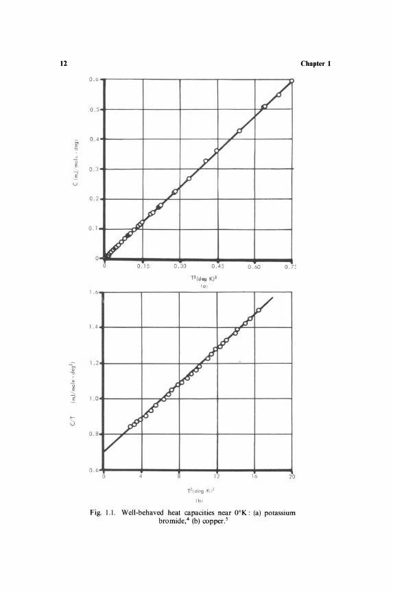
without any undetermined additive constants. Since C v is known to vanish at OOK, it is enough to measure it to a sufficiently low tempera­ture from where it may be safely extrapolated to zero. Unfortunately, the laws of thermodynamics do not give any indication of how low this temperature should be. For many solids, measurements down to liquid-helium temperature are adequate, whereas for some para­magnetic salts measurements well below 10 K are needed before a safe extrapolation is possible.

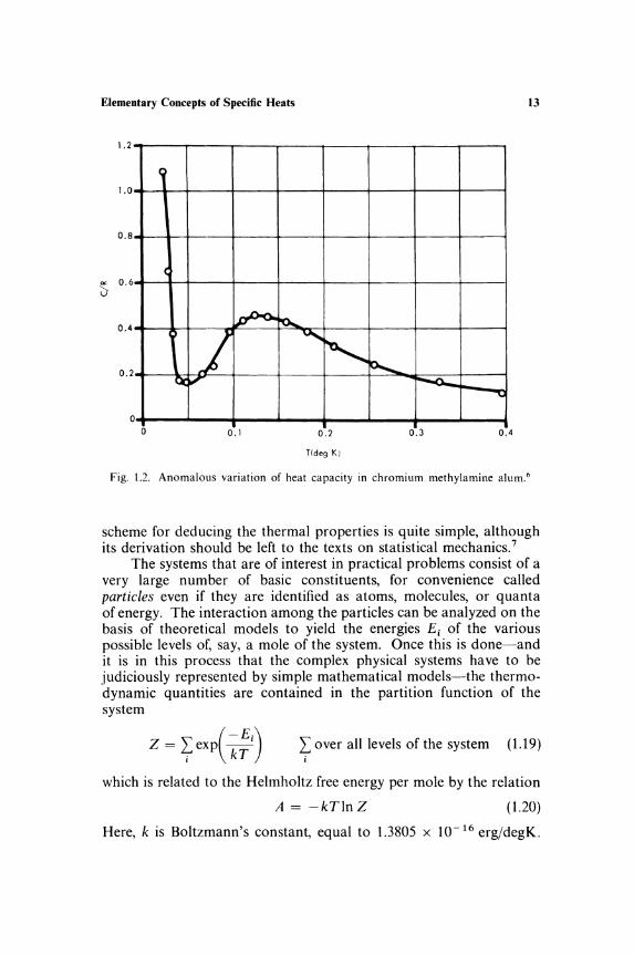
Figure 1.1 shows the specific heats of some materials near absolute zero. Dielectric solids (Figure l.la) have a low-temperature specific heat proportional to T 3, while metals (Fig. 1.1 b) obey a relation c = A 1 T3 + A 2 T. These variations are simple enough to permit a ready extrapolation of the observations to O°K. However, if the material contains paramagnetic ions-and such materials are important in adiabatic demagnetization techniques-the behavior is often quite anomalous. The specific heat of chromium methylamine alum, 6 shown in Fig. 1.2, is not falling off to zero even at O.l OK. Instead it appears to be increasing as the temperature is lowered! No doubt the specific heat will eventually tend to zero as T ..... 0, but it is quite impossible to guess its behaviour from, say, 0.5°K. It is also noteworthy that because of the low temperatures the entropy associ­ated with these anomalous variations is often large (of the order of R per mole).

1.5. STATISTICAL CALCULATION OF SPECIFIC HEATS

The examples of Fig. 1.1 and 1.2 serve to illustrate the fact that while thermodynamics is powerful in specifying the general laws governing a phenomenon it does not give any clue about the detailed behavior. This belongs to the realm of statistical mechanics, and in the following chapters it will become abundantly clear that a variety of effects observed in the behavior of specific heats may indeed be satisfactorily explained. In statistical thermodynamics, the general

12

il' ."

~ 0 E

j u

~ .. ." .. "0 e

~ .... " u

0.6

0.5 / V

0._

0.3

0.2

0 . 1

0

/ /

V

~ V

~ /

/ o 0. 15 0.30 0.60 0.75

1.6.4r------~r_------~------_r------_,------_,

1.4 ~------~--------+_------~--_r~_+------_4

1.2

1.0

O.S

0.6"'--~~---+---+-__ -+ ___ '" o 12 16 20

Fig. 1.1. Well-behaved heat capacities near OOK: (a) potassium bromide,4 (b) copper. s

Chapter I

Elementary Concepts of Specific Heats 13

1.2

~ 1.0

0.8

(

'" 0.6 ;:,

0.4

0.2

~ 1'00..

j v...... ~ P--......

Or:: ~ ~ -C

0 o 0.1 0.2 0.3 0.4

Hdeg KJ

Fig. 1.2. Anomalous variation of heat capacity in chromium methylamine alum. 6

scheme for deducing the thermal properties is quite simple, although its derivation should be left to the texts on statistical mechanics. 7

The systems that are of interest in practical problems consist of a very large number of basic constituents, for convenience called particles even if they are identified as atoms, molecules, or quanta of energy. The interaction among the particles can be analyzed on the basis of theoretical models to yield the energies Ei of the various possible levels of, say, a mole of the system. Once this is done-and it is in this process that the complex physical systems have to be judiciously represented by simple mathematical models-the thermo­dynamic quantities are contained in the partition function of the system

(-E.) z = ~exp kT' I over all levels of the system (1.19) i

which is related to the Helmholtz free energy per mole by the relation

A = -kTln Z (1.20)

Here, k is Boltzmann's constant, equal to 1.3805 x 10~ 16 erg/degK.

14 Chapter 1

It is now a simple matter to get from A

S = _(aA) E = kT2(a In Z) aT v aT I'

(a2(k TIn Z)) C" = T aT2 " (1.21)

These are the thermodynamic quantities of interest, and they are easily calculated if the partition function is set up in a convenient form.

Clearly, the specific heat at constant volume is the quantity that arises naturally in the theoretical analysis. The experimental measure­ment of Cv is possible in gases under favorable conditions because the pressures encountered, of the order of atmospheres, can be balanced by the walls of the container. For liquids and solids, on the other hand, the pressures needed to keep the volume constant run into thousands of atmospheres, and normally balancing such pressures is not practicable. Therefore, measurements are ordinarily done at constant pressure and C v is calculated from equation (1.14). The difference C p - C v is usually less than a few percent at low tempera­tures, unless the substance is near a phase transition.

1.6. DIFFERENT MODES OF THERMAL ENERGY

The above discussion underlines the fact that the heat capacity of a substance is governed by the manner in which the internal energy is distributed among its constituents. The molecules in a gas can have translational, rotational, vibrational, and electronic energy levels, and each type of thermal motion contributes its share to the specific heat of a gas. The atoms in a solid are usually held fixed at their lattice sites and can at most vibrate about their mean positions. This motion is called the lattice mode of thermal excitation. If the lattice consists of molecules, there are motions of atoms within the molecules besides the vibrations involving molecules as units. These internal vibrations may be described as molecular modes. There may be free electrons wandering through the lattice, as in metals, and the electronic contribution to C v arises from the thermal excitation of these electrons. In some cases, the energy levels of bound electrons may be split into discrete levels. The transitions among the levels are known as excitation modes. Yet another complication is that in some cases the probability of exciting some mode of thermal agitation depends strongly upon the number of particles already excited. Excitations of the particles therefore increase extremely rapidly, as though by positive feedback, once the first of such modes are excited; these snow-balling processes are called cooperative phenomena.

The contributions from all these modes have to be added together to get the total heat capacity. This may be easily seen, since to a

Elementary Concepts of Specific Heats 15

first approximation the energy of a system is the sum of the energies due to the various modes of motion. An inspection of equation (1.19) shows that the partition function is the product of factors associated with each mode. For example, the partition function Z of a gas is the product

Z = ZtZrZvZe (1.22)

of the translational, rotational, vibrational, and electronic functions. A involves In Z, which is the sum of In Z" In Zr' etc., and it is clear that the thermodynamic quantities are the sums of the contributions from the various modes.

While all these possible types of thermal agitation give their share to the heat capacity of the substance, the observed specific heat depends also upon their variation with temperature. Some of the modes are excited over the entire temperature range and so con­tribute observable specific heat at all temperatures. The atoms in a lattice can vibrate at all temperatures, and the lattice contribution to heat capacity is significant at all temperatures. It falls off as T3 when OOK is approached, as shown in Fig. l.1a. The free electrons in a metal have very high heat content, but this varies so little with temperature that its contribution to specific heats is overshadowed by the lattice term at room temperature. However, the electronic specific heat, varying as the first power of T, becomes important at liquid-helium temperature, as was seen in Fig. Lib.

In contrast to these types of thermal excitation, there are some modes which are excited over a restricted range of temperatures and so contribute an appreciable specific heat over that small range only. Typical is the excitation of energy in a system with two levels approx­imately kTo apart. At temperatures much below To, the thermal energy is insufficient to cause many excitations, as T", To transitions can occur freely, while at much higher temperature the levels are equally populated and little change in energy is possible. Hence, the specific heat is significant only in the region T '" 10 and is usually detected as a sharp bump superimposed on the other specific-heat contributions. Such behavior is called a specific-heat anomaly; Fig. 1.2 shows a good example. The hump at about 0.1 OK is due to the transitions among the energy levels of the paramagnetic ions. The substance chrome methylamine alum, Cr(NH3CH3) (S04h·12H2 0, is peculiar in showing another nearby anomaly. The sharp peak at O.02°K is caused by a cooperative transition from a paramagnetic state to an ordered antiferromagnetic state.

Any theory of solids, liquids, or gases must take into account the different types of thermal agitation, and so must lead in the first place to the energy levels of the system. The calculation of heat

16 Chapter 1

capacities involves no further assumptions. It is thus a special feature of the specific-heat studies that they provide a first ready test of the theory. However, the specific heat is only an averaged quantity; consequently, the full details of the energy levels are not usually elucidated unless the measurements are supplemented by the investiga­tions of other properties of the substance. This interplay among the different properties of the systems will become evident in the later chapters, where the heat capacity due to the various modes of thermal agitation will be analyzed with the help of suitable simple models. Before proceeding to this, it is convenient to indicate how the specific heats are experimentally determined. Only an outline of the experi­mental methods will be given here, since the matter is taken up comprehensively in a forthcoming monograph in this series.

1.7. CALORIMETRY

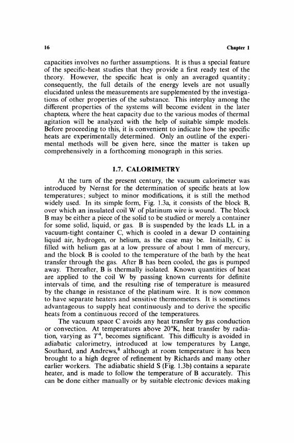
At the turn of the present century, the vacuum calorimeter was introduced by Nernst for the determination of specific heats at low temperatures; subject to minor modifications, it is still the method widely used. In its simple form, Fig. 1.3a, it consists of the block B, over which an insulated coil W of platinum wire is wound. The block B may be either a piece of the solid to be studied or merely a container for some solid, liquid, or gas. B is suspended by the leads LL in a vacuum-tight container C, which is cooled in a dewar 0 containing liquid air, hydrogen, or helium, as the case may be. Initially, C is filled with helium gas at a low pressure of about 1 mm of mercury, and the block B is cooled to the temperature of the bath by the heat transfer through the gas. After B has been cooled, the gas is pumped away. Thereafter, B is thermally isolated. Known quantities of heat are applied to the coil W by passing known currents for definite intervals of time, and the resulting rise of temperature is measured by the change in resistance of the platinum wire. It is now common to have separate heaters and sensitive thermometers. It is sometimes advantageous to supply heat continuously and to derive the specific heats from a continuous record of the temperatures.

The vacuum space C avoids any heat transfer by gas conduction or convection. At temperatures above 20°K., heat transfer by radia­tion, varying as T\ becomes significant. This difficulty is avoided in adiabatic calorimetry, introduced at low temperatures by Lange, Southard, and Andrews,8 although at room temperature it has been brought to a high degree of refinement by Richards and many other earlier workers. The adiabatic shield S (Fig. 1.3b) contains a separate heater, and is made to follow the temperature of B accurately. This can be done either manually or by suitable electronic devices making

Elementary Concepts of Specific Heats 17

1-

LU D

r/. ')-_-(1 - \ / -

............... .....f.

r- C -C

f- C

8

,-+,++- w - 5

- =-- .. -

o fbI

Fig. 1.3. Vacuum calorimeter and its modifications.

use of differential thermocouples between Band e to observe any temperature difference between them. In the liquid-helium range, a different problem arises because the helium gas used for precooling B is strongly absorbed on the surfaces of Band C. The vacuum is thereby spoiled, and even with fast pumps it may take a few hours to dislodge all the helium gas. So it is preferable to avoid the helium exchange gas altogether, though this necessitates alternative provi­sions for cooling the block B to low temperatures. In a simple form, a polished metal plate J (Fig. l.3c), which can be operated from outside the cryostat and which is in good thermal contact with e, is made to press firmly against a similar polished metal disk attached to B. e remains evacuated throughout the operation. The drawback in this technique is that when the difference in temperature between Band e is small, especially at low temperatures, heat transfer across the mechanical contact becomes very inefficient. Several cryostats, ingeniously designed to minimize these and other difficulties, are described by White9 and Hill. lO These and other books 11 .12 contain a full account of the general cryogenic techniques.

The above method is useful for measuring the specific heat above about 10 K. Below this temperature, one has to use the 3He isotope as a coolant (up to about O.3°K), or use adiabatic demagnetization to attain low temperatures. The details of these refrigeration tech­niques are described in several texts.9.10.12 Mention need be made

18 Chapter 1

here only of some special methods of finding specific heats in particular cases. Below 10 K, the heat capacity of the demagnetization pill used to cool the specimen becomes large compared to the heat capacity of the specimens. One way of avoiding this interference is to pass a p'eriodic heat-wave through the specimen and to derive Cp as in the Angstrom method of finding diffusivity at room temperatures. 13 For magnetic materials, specific heats may be obtained from studies of paramagnetic relaxation or demagnetization from various magnetic fields (Chapter 4).

In the case of gases, measurements made by having the gas in a closed container, as originally done by Eucken and others for hydro­gen, yield Cv directly, because the volume change under such condi­tions is very small. The specific heat at constant pressure can be determined by continuous-flow methods as at room temperatures. Information about Cv in gases may be obtained from the heat conduc­tion when the mean free path becomes comparable to the dimensions of the measuring apparatus. Moreover, the ratio of specific heats Cp/Cv may be determined from the velocity of sound in gases (Sec­tion 8.3). A good survey of the measurement of specific heat in gases is given by Rowlinson. 14

There are many problems associated with thermometry and heat leakages, the details of which are discussed in several reviews. 1 5.16,17

A point often overlooked is the need for pure specimens. Parkinson16

has listed a number of anomalous results originally reported in such common materials as sodium, mercury, beryllium, germanium, etc., which had been puzzling and which have now proved to be not characteristic of the pure materials. When it is realized that at 0.1 OK chrome methylamine alum has a molar heat capacity nearly 40,000 times that of copper, it is obvious that even traces of impurities may sometimes vitiate calorimetric measurements.

REFERENCES 1. M. W. Zeman sky, Heat and Thermodynamics, McGraw-Hill, New York, 1957.

J. K. Roberts and A. R. Miller, Heat and Thermodynamics, Blackie, London, 1960. 2. H. B. Huntington, Solid State Phys. 7, 213 (\958). R. F. S. Hearmon, Introduction

to Applied Anisotropic Elasticity. Oxford University Press, Oxford, 1961. 3. R. Viswanathan and E. S. Raja Gopal, Physica 27, 1226 (\961). 4. H. R. O'Neal, Ph.D. thesis (unpublished), University of California, 1963. 5. J. A. Rayne. Austral. J. Phys. 9, 189 (\956). K. G. Ramanathan and T. M.

Srinivasan, J. Sci. lndustr. Res. 168,277 (1957). 6. W. E. Gardner and N. Kurti, Proc. Roy. Soc. (London), Ser. A 223, 542 (\954). 7. C. Kittel, Elementary Statistical Physics, Wiley, New York, 1958. D. K. C.

MacDonald. Introductory Statistical Mechanics for Physicists, Wiley. New York, 1963.

8. F. Lange. Z. Phys. Chem. 110. 343 (\ 924). J. C. Southard and D. H. Andrews, J. Franklin Inst. 209. 349 (1930).

Elementary Concepts of Specific Heats 19

9. G. K. White, Experimental Techniques in Low Temperature Physics, Clarendon, Oxford, 1959.

10. F. E. Hoare, L. C. Jackson, and N. Kurti, Experimental Cryophysics, Butterworth, London, 1961.

II. F. Din and A. H. Cockett, Low Temperature Techniques, Newnes, London, 1960. 12. A. C. Rose-Innes, Low Temperature Techniques, English University Press, London,

1964. 13. D. H. Howling, E. Mendoza, and J. E. Zimmerman, Proc. Roy. Soc. (London),

Ser. A 229, 86 (1955). N. V. Zavaritsky, Progr. Cryogenics 1, 207 (1959). 14. 1. S. Rowlinson, The Perfect Gas, Pergamon, Oxford, 1963, chapter 2. 15. P. H. Keesom and N. Pearlman, Handbuch der Physik, XIV(l), 282 (1956). 16. D. H. Parkinson, Rept. Progr. Phys. 21, 226 (1958). 17. R. W. Hill, Progr. Cryogenics 1,179 (1959). W. P. White, The Modern Calorimeter,

Chern. Pub. Co .. New York. 1928. J. M. Sturtevant, in: A. Weissberger (ed.), Physical Methods of Organic Chemistry. Part I, Interscience. New York. 1959. chapter 10.

Chapter 2

Lattice Heat Capacity

2.1. DULONG AND PETIT'S LAW

One of the earliest empirical generalizations concerning the specific heat of solids was enunciated by Dulong and Petit in 1819. Its theoretical justification was advanced by Boltzmann in 1871, and in 1907 Einstein showed why it failed at low temperatures. These dates are among the principal landmarks in the study of specific heats. To appreciate the significance of these developments, consider the specific heats of several common elements at room temperatures, as collected in Table 2.I. The specific heat per gram of the element varies considerably, being small for the elements of high atomic weight and large for those of low atomic weight. However, the heat capacity per gram-atom of all of them is nearly equal to 6.2 caI/mole'deg,

Table 2.1. Specific Heat of Solid Elements at Room Temperature!

Element

Bi Pb Au Pt Sn Ag Zn

cp 0.0299 0.0310 0.0309 O.03IS 0.0556 0.0559 0.0939 Atomic

weight 209.0 207.2 197.0 195.1 IIS.7 107.9 65.4 Cp 6.22 6.43 6.10 6.21 6.60 6.03 6.14

Cu Fe AI Si B C(gr) C(di)

cp 0.0930 0.110 0.21S 0.177 0.26 0.216 0.12 Atomic

weight 63.6 55.9 27.0 2S.1 IO.S 12.0 12.0 Cp 5.92 6.14 5.S3 5.00 2.S4 2.60 1.44

Cp in caljmoie'deg, Sn = grey tin, C(gr) = graphite, C(di) = diamond.

20

Lattice Heat Capacity

NaCl

Table 2.11. Molar Heat Capacity of Compounds 1

(in caljmole·deg)

Compound

KBr AgCl PbS

C p 11.93 12.25 12.15 12.01 12.33 17.83 18.05 16.56 27.2

21

which is the rule found by Dulong and Petit in 1819. A closer inspec­tion shows that for "light and hard" elements (silicon, boron, and carbon) the atomic heat capacity falls much below the Dulong-Petit value.

Subsequent experiments by several workers during the period 1840 to 1860 revealed an important extension of the Dulong-Petit rule. The molar heat capacity of a compound is equal to the sum of the atomic heat capacities of the constituent elements. Table 2.11 illus­trates this rule, which is sometimes called the law of Neumann and Kopp. Diatomic solids have a molar specific heat of approximately 12caljmole'deg, while triatomic solids have C p ~ 18 units. As in Table 2.1, there are many substances that deviate greatly from this simple behavior, but on the whole there is enough evidence for taking the atomic specific heat to be about 6 cal, irrespective of the chemical structure of the substance. Since the gas constant R = Nk has a value of approximately 2 caljmole'deg, this statement implies that each atom in a solid contributes about 3k to the specific heat.

2.2. EQUIP ARTITION LAW

The empirical results of the previous section can be readily interpreted on the basis of the theorem of equipartition of energy developed by Boltzmann. A derivation of this theorem may be found in the texts on statistical mechanics or in other places. 2 ,3 In classical mechanics, a system executing small oscillations may be described in terms of normal coordinates; its energy is then expressed as the sum of several squared terms. For example, the energy of a linear har­monic oscillator is made up of kinetic and potential energies (2m)-lp2 + imw2q2, where p is the momentum and q the coordinate. For a three-dimensional oscillator there are three p;, p;, p; terms and three q;, q;, q; terms. Each such square term in the energy expression is said to arise from a degree of freedom of the system, which is nothing more than an enumeration of the independent variables needed to describe the system. The equipartition law states

2Z Chapter 2

that in thermal equilibrium each degree of freedom contributes !kT to the energy of the particle. Thus, a three-dimensional oscillator has an internal energy 3kT when a system of such oscillators is in thermal equilibrium.

The atoms in a solid are arranged in a regular lattice and held in their lattice sites by interatomic forces acting on them. A simple model of a lattice would be a set of mass points connected to one another by elastic springs. The atoms can vibrate about their mean positions under the influence of the forces acting on them, and if the amplitude of oscillation is small, the atoms may be considered as harmonic oscillators. Each (three-dimensional) oscillator has six degrees of freedom, and by the equipartition theorem has an internal energy 3kT. In a gram-atom of the element there are N atoms and the internal energy is 3NkT. Therefore, the heat capacity is Cv = iJE/iJT = 3R ~ 5.96 caljmole·deg. For a compound with r atoms per molecule, the molar heat capacity is 3rR.

Classical statistical mechanics is thus able to justify the empirical observation of Dulong and Petit and others. The successful theoreti­cal explanation of the heat capacity of solids (and of gases, which will be discussed in Chapter 6) was, at that time, partly instrumental in the acceptance of molecular mechanisms not only for mechanical properties but also for thermal properties of matter, a fact which is taken for granted nowadays.

A perusal of Table 2.1 shows, however, that for some substances the heat capacity is much less than the equipartition value. Experi­ments performed above room temperature revealed that at high temperatures the heat capacity of even these substances increases to 3R. For example, diamond, which had Cp '" 1.4 caljmole'deg at 300oK, had C p '" 5.5 units at 1200°K. On the other hand, when cryogenic experiments were performed, it was found that the specific heat of all materials decreased at low temperatures. Illustrative is the behavior of copper with C p '" 5.9 caljdeg at 3000 K and '" 3.9 units at 100°K. At 4 oK, its value is only 1/4000 of the equipartition value! Classical statistical mechanics could offer no cogent explanation whatsoever for such large temperature variations of specific heats. The clarification had to await the development of quantum theory.

2.3. QUANTUM THEORY OF SPECIFIC HEATS

In 1901, Planck was forced to conclude from his studies on the spectral distribution of blackbody radiation that the energy of an oscil­lator of frequency v must change in discrete steps of hv, and not con­tinuously, as had been assumed in classical mechanics. The constant h, called Planck's constant, has a value of 6.626 x 10- 27 erg-sec.

Lattice Heat Capacity 23

Einstein soon realized that electromagnetic radiation travels in packets of energy hv and momentum h/A; these wave packets have come to be called photons. Finally, in 1907, Einstein took the bold step of applying quantum theory outside the field of electromagnetic radia­tion to the thermal vibrations of atoms in solids. The floodgates had been opened for quantum concepts to pervade the whole of our physical knowledge.

Before going into the details of the theory, it is best to grasp the simple implications of the quantization of energy. It was known even in 1907 that the atomic vibrations in a solid have frequencies of the order of 1013 cps. The energy hv needed to excite such a vibra­tion is approximately 6.6 x 10- 14 erg. In a naIve way, if this is equated to the classical energy of an oscillator 3kTo, then To comes out to be 150°K. At high temperatures, the atomic vibrations will be excited fully, but below about 1500 K the vibrations cannot be excited because the minimum energy needed for this process is not available. Hence, the specific heat should drop from its classical equipartition value to zero below about 150°K. In practice, the reduc­tion will not be so abrupt as in this naIve picture, because at any temperature above OaK there is a statistical probability of exciting some vibrations, given by the Boltzmann factor exp (- hv/kT). The effect of lowering the temperature is to reduce the number of excita­tions, and in this manner the quantization of energy levels brings about a reduction of specific heats at low temperatures.

The formal way of handling the problem, as outlined in Section 1.5, is to calculate the partition function Z and the Helmholtz free energy A:

A = -kTlnZ Z = ~ exp ( ~:i) (2.1)

An atom in a lattice vibrates under the influence of the forces exerted on it by all the other atoms of the system. If the amplitude of the vibrations is small, classical mechanics shows that the vibrations can be resolved into normal modes, i.e., into a set of independent one­dimensional harmonic oscillations. In a mole of the substance, the molecules of which contain r atoms, there are 3rN such independent modes. The total energy is the sum of their energies, and the total partition function is the product of the 3rN modes:

Zsystem = IIzmode

Detailed quantum-mechanical considerations show that the energy levels of a linear oscillator are given by Sn = (n + !)hv, the !hv being the zero-point energy. Then, summing up the geometrical

24 Chapter 2

series,

Lx (-en) exp( -thv/kT) 1 h(thV) z = exp -- = = "2 esc -kT 1 - exp( - hv/kT) kT

n= 0

(2.2)

Now the number of modes in a crystal is so large, of the order of 1023/cm3 , that it is advantageous to write

NUMBER OF MODES BETWEEN FREQUENCIES V AND V + dv = 3rNg(v) dv (2.3)

Obviously, the total number of modes is 3rN, so that

( g(v)dv = 1 (2.4)

With the distribution of frequencies g(v), equation (2.1) becomes

A = 3rNkT fin [2 sinh(t~)Jg(V) dv

= Eo + 3rNkT J: In [1 - exp( ~;v)Jg(V) dv (2.5)

where

Eo = t3rN J~ hvg(v) dv

is the zero-point energy of the solid. The calculation of the specific heat is now straightforward, and it may be verified that

C v = - TG~~) v = 3rNk J: (t~ Y CSCh2( t~) g(v) dv (2.6)

This general introduction serves several purposes. For the sake of simplicity, the later calculations of specific heats will start from a discussion of the mean energy of the particles. In satisfying the didactic exigencies, it should not be forgotten that a pedestrian derivation from first principles is possible. Secondly, in some of the discussions it will not be obvious whether P or V is held constant, that is, whether Cp or Cv is calculated, mainly because there is no thermal expansion if harmonic vibrations are assumed. The above derivation makes it clear that only Cv is calculated. Thirdly, the thermodynamics of crystals has been reduced to the evaluation of the distribution of frequencies g(v). The determination of g(v) is a dyna­mical problem of great complexity, and it is best to introduce the subject with the simple models proposed by Einstein (1907), Debye (1912), and Born and Von Karman (1912).

Lattice Heat Capacity 25

2.4. EINSTEIN'S MODEL

Einstein, in his fundamental paper, considered a very simple model of lattice vibrations, in which all the atoms vibrate inde­pendently of one another with the same frequency VE. In a substance such as copper, for instance, an atom has the same environment as any other atom, and it is plausible to suppose as a first approxima­tion that all atoms vibrate with the same frequency VE • If that were so, g(v) would be zero for v #- V E and nonzero for v = VE • Then equation (2.6) immediately gives

C = 3rNk(thVE)2 CSCh2(thVE) v kT kT

(2.7)

which is Einstein's well-known relation. It is, however, instructive to derive the same relation by a dif­

ferent method. The atoms in a solid vibrate about their mean posi­tions, and for such localized particles Maxwell-Boltzmann statistics is applicable. This means that the probability of exciting an energy e at an equilibrium temperature T is proportional to exp( - e/kT). According to quantum theory, the energy levels of an oscillator v are given by en = (n + t)hv. In thermal equilibrium, the probability that a given oscillator will be in the energy state en is proportional to the Boltzmann factor exp( -ejkT), and so the average energy of the oscillator is

L. en exp( -ejkT) L. ne- nx

£ = n = thv + hv---L. exp( -ejkT) L. e- nx

where x = hv/kT. Now

L. ne- nx d d 1 1 L. e nx = - dx In I e - nx = - -In dx 1 - e- x eX - 1

Therefore, at a temperature T, the mean energy of the oscillator is

hv £ = thv + -----­

exp(hv/kT) - 1 (2.8a)

On differentiating this, the specific-heat contribution from the oscillator is seen to be

ae kx 2ex

aT (ex -1)2 (2.8b)

26 Chapter 2

In the Einstein model, all the 3rN independent vibrations have the same frequency V E• Hence, the total internal energy is

E = 3rRT[-tXE + _X-'E'--] eXE - 1

( _ hVE) X E -kT

and the molar heat capacity is

The molar entropy is

S = 3rK - In(1 - e- XE ) [ XE ~ eXE - 1

(2.9a)

(2.7)

(2.7a)

The quantity hVE/k plays the role of a scaling factor for temperature and is called the Einstein temperature TE• The Einstein functions E(TE/T) and C,.(TE/T) are tabulated in several places4 ,5 (see also the appendices at the end of Chapter 8). A consideration of the values of exponentials in equation (2.7) at very high and very low temperatures shows that

(high temperature, T ~ TE)

(2.10)

(low temperature, T ~ TE)

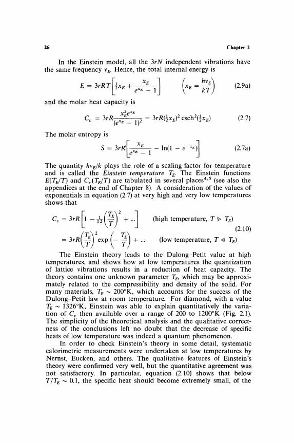
The Einstein theory leads to the Dulong~Petit value at high temperatures, and shows how at low temperatures the quantization of lattice vibrations results in a reduction of heat capacity. The theory contains one unknown parameter TE, which may be approxi­mately related to the compressibility and density of the solid. For many materials, TE ~ 200oK, which accounts for the success of the Dulong~Petit law at room temperature. For diamond, with a value TE ~ 1326°K, Einstein was able to explain quantitatively the varia­tion of Cv then available over a range of 200 to 12000K (Fig. 2.1). The simplicity of the theoretical analysis and the qualitative correct­ness of the conclusions left no doubt that the decrease of specific heats of low temperature was indeed a quantum phenomenon.

In order to check Einstein's theory in some detail, systematic calorimetric measurements were undertaken at low temperatures by Nernst, Eucken, and others. The qualitative features of Einstein's theory were confirmed very well, but the quantitative agreement was not satisfactory. In particular, equation (2.10) shows that below T /TE ~ 0.1, the specific heat should become extremely small, of the

1.0

0.8

"" ..., 0.0

~ U

0 .4

0 .2

0

Lattice Heat Capacity 27

/ ~ ~ Oebye _

I ~.in II

/ V JJ

o 0 .2 0.4 0 .0 0 .8 1.0 1. 2 1. 4 1. 6 1.8

Tie or TI TE

Fig. 2.1. Temperature variation of heat capacity in Einstein and Debye models. Original comparison of Einstein for diamond (TE = 1326°K) and of Debye for

aluminum (OD = 396°K) are shown.

order of mJ/mole' deg, whereas experimentally the decrease was much slower (Fig. 2.1). Several workers, including Einstein himself, recognized that the model was oversimplified.6 In a tightly coupled system, such as a lattice, the motion of one atom affects the vibrations of the others and the atoms can vibrate with several frequencies. Experimentally, Nernst and Lindemann pointed out that the observa­tions could be fitted better if two frequencies VE and tVE were used instead of VE alone. In the simple model, there is no provision for vibrations of low frequencies, which alone can be fully excited in the region of small energies, i.e., at low temperatures. These ideas culminated in the calculations (1912) of Debye and Born and Von Karman, who used a better description of lattice vibrational fre­quencies. Debye's model is the simpler and will be taken up in the following section.

Despite the cursory dismissal usually accorded to Einstein's oversimplified model, the calculation was a fundamental step in enlarging the field of application of quantum ideas. A great deal of experimental and theoretical work on the specific heats of solids and gases was inspired by it. Indeed, even today Einstein's calculation remains useful as a very simple approximation in many problems of the solid state and in discussion of molecular vibrations.

28 Chapter 2

2.5. DEBYE'S MODEL

The quantization of vibrational energy implies that at low temperatures only the low-frequency modes of lattice vibrations will be appreciably excited. Now the usual very-low-frequency vibrations of a solid are its acoustic oscillations. They have wavelengths much larger than atomic dimensions, and so in discussing their behavior the ideas of an elastic continuum may be borrowed. Debye calculated the distribution of frequencies which result from the propagation of acoustic waves of permitted wavelengths in a continuous isotropic solid and assumed the same distribution to hold good in a crystal, also. The use of such a g(v) turned out to be so extraordinarily success­ful in explaining the thermal behavior of solids that it merits dis­cussion in some detail.

A plane wave propagating with velocity c in an isotropic medium satisfies the equation

c2 '\1 Z¢ = a2¢ iJtZ

For convenience, take a rectangular parallelopiped of sides L1, Lz, L3,

on the faces of which the displacement amplitude is zero. Then the wave equation has a standing-wave solution of the form

¢ = A sin q1x sin qzy sin q3Z sin 2nvt

where the orders of the overtones ni are related to the wave vectors qi = 2n/}..i by

An enumeration of the values of ni which give a frequency between v and v + dv solves the problem of finding K(v)dv. In a practical case, the number of modes, approximately 1023 /cm3, is so large that the ni may well be treated as continuous variables. The number of allowed values of ni in the range ni to ni + dni is then equal to

L1LzL3 V ,1n l,1nz,1n3 = ~-3--,1ql,1qZ,1q3 = ~3,1ql,1qZ,1q3

n" n

where V is the volume of the solid. Now the frequency of the wave is

2 (qi + q~ + qncZ qZcZ v = -=-:'------=-~--"-=----

4n z 4n z

Since the ni are all positive, this is nothing but the equation for the first octant of a sphere in the q 1 q zq 3-space. The volume of the shell

Lattice Heat Capacity 29

between q and q + dq, equal to k4nq2 dq, corresponds to (V/2n2) q2 dq allowed values of ni . In terms of frequencies, the number of allowed modes between v and v + dv is

4nV n(v) dv = -3-V2 dv

C (2.11)

In an elastic solid, three types of waves are possible. 7 •s One is the longitudinal wave with velocity CL> for which 4h may be taken as the dilatation of a volume element. The other two are transverse shear weaves, and for them ¢ TJ, ¢T2 are the components of the rotation of a volume element. In an isotropic solid, which is being considered at first, the transverse waves have the same velocity CT. Adding the three contributions, the number of frequencies between v and v + dv in an elastic solid is

(2.12)

Considerations of simplicity necessitated a derivation of equation (2.12) for a rectangular parallelepiped, but the result is not significantly altered by considering a large body with any shape. The same remark holds good for several other distributions of energy levels considered in this book (Sections 2.8 and 6.3). Mathematical proofs of this assertion have been given in various cases. 9

Oebye suggested that the collective low-frequency oscillations of the solid given by equation (2.12) should be applied even at high frequencies and that the discrete nature of the atomic lattice should be taken into account by setting a minimum to the allowed wave­lengths. The corresponding upper limit VD to the frequency is to be obtained from the normalizing condition, equation (2.4), that the total number of modes is equal to 3rN per mole. Thus, taking the molar volume to be V,

4nV _ 3 - 3 3 -3-(CL + 2cT )vD = 3rN

or (2.13) v = (9rN)I/3(C_ 3 + 2C- 3)-1/3

D 4nV L T

For the cut-off procedure to be meaningful, the limiting wavelength should have atomic dimensions. In a typical solid, the minimum possible wavelength is

~ (4nV)I/3 ~ ( 4n x 10 ) 1/3 ~ 3A 9N 9 x 6 X 1023

which is indeed of the same order as the lattice spacing.

30 Chapter 2

The distribution of frequencies may therefore be taken as

3v 2

g(v) =-3 VD

for v :S; VD

= 0 for V> VD

(2.14)

Each wave of frequency v has an energy hv and momentum hi) .. In the quantum formulation, the lattice waves are called phonons; equation (2.14) represents the Debye approximation to the phonon spectrum of a crystal lattice (Fig. 2.5b). The characteristic temperature

is known as the Debye temperature. It is now a simple matter to check that

E = 3rN !hv + h Ik/ ---;- dv fVD [ h J 3 2

o e V_I VD

_ 9rNk(J 9rNkT4 foiT x 3 dx - 8 + (J3 eX - 1

o

9rNk(J3folT [x I (1 -X)] 2 d s= ----n -e x x T3 eX - 1

o

[4T 3JOIT X3 dx l = 3rNk 7f3 0 eX _ 1 - In(1 - e-OIT)J

fVD (hV) 2 ehvlkT 3v 2

Cv = 3rNk 0 kT (ehvlkT _ If vt dv

= 9rNkT 3JOIT x 4 ex dx (J3 (eX - If

o

_ [4T 3 fOIT x 3 dx _ (J/T ] - 9rNk (J3 X OIT 1

o e - 1 e -

These are the famous relations derived by Debye.

(2.15)

(2.l6a)

(2.16b)

(2.17)

Two general remarks are appropriate here before discussing the theory in detail. According to quantum statistics2 ,3, the smallest possible cell in the p,q-phase space (momenta Px, Py, Pz, coordinates qxqyqz) is of volume h3. In a gas of free particles contained in an enclosure of volume V, the number of allowed cells n(p) dp between momenta p and p + dp is h- 3 IH HI dpx dpy dpz dqx dqy dqz. The integration over dq is equal to V. Next, converting the integral over

Lattice Heat Capacity

dp into spherical polar coordinates,

4nV n(p) dp = yp2 dp

31

(2.18)

Considering phonons as free particles with p = hi)., this immediately gives equation (2.11). Secondly, in the preceding derivation, Maxwell­Boltzmann statistics was applied to the vibrations of localized atoms in deriving equation (2.7). Instead, one may consider a set of phonons obeying Bose-Einstein statistics and derive Debye's results. This point of view is adopted in Section 5.4 in treating a closely related problem.

2.6. COMPARISON OF DEBYE'S THEORY WITH EXPERIMENTS

The Debye model has been extremely successful in correlating the specific heats of solids. The temperature variation of Cv given by equation (2.17) is obeyed very well by a variety of substances, a typical example being given in Fig. 2.1. At high temperatures, the integrand in equation (2.17) approaches x 2 , so that

(T ~ 0) (2.19)

At very low temperatures, the upper limit of the integral may be taken as infinity, when the integral has a value 12n4/45. Thus, for T < OliO,

Cv = ? rRn4(;Y = 464.3(;Y cal/mole' deg (2.20)

= 1944(~y J/mole . deg

At intermediate temperatures, the Debye function must be evaluated numerically/o and several tables exist. 4 • 11 A comprehensive numerical tabulation is reproduced at the end of Chapter 8.

The T 3-variation at low temperatures was one of the first pre­dictions of the theory. The T 4 -variation of the internal energy is the acoustic analog of the well-known Stefan-Boltzmann law that the energy density of a photon gas is proportional to T4. Debye's pre­diction was soon verified, and the specific heat of many dielectric solids, such as rocksaIt, sylvine, fluorspar, etc., show excellent agree­ment with the theoretical law. In Fig. 1.1a, an example was given to illustrate the T 3-behavior at sufficiently low temperatures. As a

32 Chapter 2

matter of fact, the T 3-law is so universal at very low temperatures that it has found a permanent place in the theory of specific heats, although the range of validity has now been restricted to T < 8/50 on account of more recent theoretical work to be described later.

Apparent deviations are found in some cases for rather obvious reasons. Graphite, boron nitride, and other layered materials, which behave like two-dimensional crystals, show a T 2-variation at some temperatures. Similarly, long-chain molecules such as sulfur and some organic polymers exhibit a variation linear in T at some tem­peratures, as pointed out by Tarasov and coworkers. Even in these cases, detailed calculations show that at sufficiently low temperatures a T 3-law should be present, and such measurements have been carried out recently. 12

Over wide ranges of temperature, the Debye theory has the note­worthy and attractive feature of making the specific heat depend upon a single parameter 8. Therefore, with a suitable choice of the temperature scales, the heat capacities of all substances should fall on the same curve. Schrodinger 13 and later Eucken 1 reviewed the specific-heat data available prior to 1928 and found extraordinarily good agreement with Debye's theory. Figure 2.2, adapted from Schrodinger's review, makes the excellence of the agreement self­evident. Striking agreements such as this have resulted in a wide­spread application of Debye's theory to a variety of solid state problems, some of which will be mentioned in Section 2.11.

___ T.

0.2 0.30.' O.S 0.6 0 . 7 0 .80.9 I 1.1 1.21.3 1. 4 I.S 1.61.71.8 1.9 2 2.1 2.22.32.4 2.S 2.6

Cd ~ ~---,,-~.-. -+ a a rl;,x . ;p,.-11 .60 a . o • III ;II:

• .; •• -...JL.....o ... ~og-"-J( "'o~ 6 - "-"'--,....-I'-~. . --...---.

~.~... • "" KCI Z oCI C, AI Cof, C .c t. O ~ .. Pb n

I /~~--- " ""I'---'- ' - '- --- -- ­~ 3 /1 ,4 !.! I : J~ II°./zn ! ~ . f If , F.

1 AI I Cof, I F.s, fcu i KCI

aCI .

--T, 2.1 2.2 2.32.' 2.S 2.6

Fig. 2.2. Heat capacities of several substances (in cal/mole'deg) compared with Debye's theory. For the sake of clarity, portions I and III are shown shifted.

Lattic:e Heat Capacity 33

It will be seen later that small deviations from the theory are found and that if at each temperature the specific heat is fitted to a Debye term then the resulting values of e vary slightly with tempera­ture. 14 In a good many cases, the variation of e from its mean value is less than about 10 %, though a few exceptions, for instance, zinc and cadmium, show variations of more than 20 %. For a preliminary calculation of specific heats, a list of Debye characteristic tempera­tures, as given in Table 2.111, can be used with complete confidence. The values given in Table 2.111 have been taken at T - e12, which gives a reasonable fit over most of the specific-heat curve. 10 In Chapter 3, e values of some metals are given, but there e refers to eo, the value at very low temperatures, since the specific-heat data at very low temperatures are involved.

Table 2.111. Debye Characteristic Temperatures of Some Representative Elements and Compounds (in deg K at T - e 12)

Element (J Element 0 Element (J Element

A 90 Dy 155 Mg 330 Sb Ac 100 Er 165 Mn 420 Se Ag 220 Fe 460 Mo 375 Si AI 385 Ga(rhom) 240 N 70 Sn (fcc) As 275 Ga (tetra) 125 Na 150 Sn (tetra) Au 180 Gd 160 Nb 265 Sr B 1220 Ge 370 Nd 150 Ta Be 940 H (para) 115 Ne 60 Tb Bi 120 H (ortho) 105 Ni 440 Te C(diamond) 2050 H (n-D 2 ) 95 0 90 Th C (graphite) 760 He 30 Os 250 Ti Ca 230 Hf 195 Pa 150 TI Cd (hep) 280 Hg 100 Pb 85 V Cd (bee) 170 I 105 Pd 275 W Ce 110 In 140 Pr 120 Y CI 115 Ir 290 Pt 225 Zn Co 440 K 100 Rb 60 Zr Cr 430 Kr 60 Re 300 Cs 45 La 130 Rh 350 Cu 310 Li 420 Rn 400

Compound (J Compound (J Compound () Compound

AgBr 140 BN 600 KCI 230 Rbi AgCI 180 CaF2 470 KI 195 Si02 (quartz) Alums 80 CrCI 2 80 LiF 680 Ti02 (rutile) As2O) 140 CrCI) 100 MgO 800 ZnS As2O, 240 Cr2O) 360 MoS 2 290 AuCu) (ord) 200 FeS2 630 NaCI 280 AuCu) (disord) 180 KBr 180 RbBr 130

()

140 150 630 240 140 170 230 175 130 140 355 90

280 315 230 250 240

()

115 255 450 260

34 Chapter 2

A fundamental feature of Debye's theory is the connection between elastic and thermal properties of substances. The charac­teristic temperature () may be determined from the velocities of longitudinal and transverse sound waves, using equations (2.13) and (2.15). In crystals, a complication arises because the velocity of elastic waves depends upon the direction of propagation in the aniso­tropic medium. In general, the three modes have different velocities and are not separable into pure longitudinal and pure shear modes. 7,8

It is then convenient to define a mean velocity

3(2)~ 1 = cZ 3 + 2c y3 = (4n)~ 1 f L Ci~3 dO i= 1,2,3

where dO is an element of solid angle in which the velocities are c1, c2 , C3 . Various approximate procedures for calculating the mean velocity in terms of the elastic constants are reviewed by Blackman 1 0

and Hearmon. 7 Table 2.IV gives some values of () originally calcu­lated by Debye from the elastic constants of polycrystalline materials. A comparison with the calorimetric results at moderate temperatures reveals a surprisingly good agreement in spite of the uncertainty in the elastic constants. Equation (2.13) gives a dependence of () upon the density of the substance; in the case of solid helium-four and solid helium-three, which are highly compressible, () can be changed by as much as 30 % with a moderate pressure of about 150 atm. Another good example is the dependence of () upon the isotopic mass of the atom, which is easily observable in lithium isotopes of masses 6 and 7. The experimental difference 15 of 9 ± 2 % is in quantitative agreement with the theoretical estimate of 8 %. Such a correlation of the thermal and mechanical properties of solids must be considered a great triumph of the theory.

In view of these remarkable successes, the Debye theory has found a permanent niche in solid state physics. It is based on a simple and understandable model. Cv is expressed in terms of a single parameter () and is in reasonably good agreement with experi­mental values. The predicted T 3-behavior is verified at low tempera-

Table 2.IV. Comparison of ()-Values from Calorimetric and Elastic Data at Room Temperature

Substance

£I-value Al Cu Ag Au Cd Sn Pb Bi Pt Ni Fe

Elastic 399 329 212 166 168 185 72 111 226 435 467 Calorimetric 396 313 220 186 164 165 86 111 220 441 460

Lattice Heat Capacity 3S

tures. Further, the theory allows a satisfactory correlation of the calorimetric measurements with elastic and other properties of the substance.

2.7. SHORTCOMINGS OF THE DEBYE MODEL

The great popularity of Debye's theory of specific heats should not blind us to its defects. The first hint that all was not well with the theory came from the early observations of Eucken, Griineisen, and others that if 0 was calculated from the low-temperature elastic constants, the agreement with the thermal values became worse instead of better. For instance, in aluminum, O(elastic) is 399°K at room temperature and 426° at OOK (Tables 2.1V and 2.V), while O(thermal) is 396°. Further, 0 as deduced from the T3-law [equation (2.20)] did not always agree with the value needed to fit the whole of the specific-heat curve. This dilemma was resolved only after the development of the lattice theory.

When accurate values of specific heats at low temperatures became available with improved calorimetric techniques, it was found that equation (2.17) for Cv did not fit the experimental results exactly. This is usually demonstrated by calculating the effective values of 0 necessary to fit the experimental data with equation (2.17) at each temperature. Of course, if Debye's model is really correct, a constant value of 0 should be obtained, but in practice this is not SO.14 Often, as the temperature is lowered the effective value of 0 begins to decrease slightly around 0/2, has a minimum, and then rises to attain a constant value below 0/50. Thus, at temperatures well below 0/50 and above 0/2, the theory works well, with a different O-value in each range. Figure 2.3 shows a recent study of the 0-T dependence in sodium iodide. 16 At one time, such deviations were attributed to experimental errors, impure specimens, and other extraneous causes, but since the theoretical work of Blackman in 1937, to be discussed below, it has been known that these deviations are genuine.

The fundamental deficiency in the Debye model is the inade­quate treatment of the effects arising from the discreteness of atomic arrangements in the crystal. The periodicity of the lattice causes the medium to be dispersive; that is, the velocity of propagation of the lattice wave is a function of the frequency. This phonon dispersion was correctly taken into account in the model proposed by Born and Von Karman in the same year (1912) as Debye's work. However, the lattice model resulted in cumbersome mathematics, and Born and Von Karman's original calculation did not give as good a fit with experiments as Debye's simpler analysis. Hence, the application of lattice dynamics (which Born continued to develop in connection

36

200

180

o o

00

o 0 cPoo 0

o tP L.2.--o_ o_­~-o-oo

tfPJ!i(p0,J9 orf'oo 00 o

/~ 0

~ ! 0.2:110 f C"

( P o

. • • o

o o

Chapter 2

Q

B' ~ 160 I

t 2~ 1 ole" 150 o

o CD

• o • r o

140

·0 'i'* ,,~,

o 30

o

T(deg K)

Fig. 2.3. Variation of effective Debye temperature () with T for sodium iodide. 16

with other problems in solid state) to the question of specific heats lay dormant until Blackman's analysis showed its fundamental significance. 17

2.S. THE BORN-VON KARMAN MODEL

A complete enumeration of the vibrational modes of a three­dimensional lattice involves formidable computations, as will become obvious later. In an elementary text, it is not practicable to go into these details, and so only the simplified case of a one-dimensional lattice will be considered. It turns out that a linear monatomic lattice does not exhibit one of the characteristic features of a three-dimen­sional crystal, namely, the presence of optical modes. Therefore, the simplest illustrative case is that of a linear diatomic lattice.

Lattice Heat Capacity 37

To visualize the effects caused by the atomic structure of crystals, consider a one-dimensional chain with two kinds of atoms, spaced a apart. Atoms of mass m are placed at even lattice points ... 2na, (2n + 2)a, ... , while masses M are at odd sites ... (2n - l)a, (2n + l)a, .... For simplicity, assume further that each atom interacts only with its two neighbors so that a relative displacement Un+! - Un causes a force f3(un+! - un) to act on atom n. Then the equations of motion for the 2n and 2n + 1 particles are

mU1n = f3(u1n + 1 - U1n + Uln-! - U1n)

Mu1n +! = f3(U1n +1 + U1n - 2u1n + d The boundary conditions do not significantly alter the distribution of frequencies,9 and so the solutions may be taken in the simple form

Uln = ~ exp i(wt + 2nqa)

U1n +! = IJ exp i[wt + (2n + l)qa]

Substituting in the equations of motion,

-wlm~ = I3IJ(e iqa + e- iqa) - 2f3~

-w1MIJ = f3~(eiqa + e- iqa) - 2f3IJ

(2.21 )

(2.22)

The condition that there are nonzero solutions ~,IJ describing a wave is that the determinant of the coefficients must vanish:

or

-213 cos qa =0 (2.23a)

-213 cos qa

w1 = f3(M-! + m-!) ± f3[(M-! + m-!)l - 4M-!m-! sinlqa]1/1 (2.23b)

The two roots correspond to two different branches of the frequency-wave vector relationship, which is shown in Fig. 2.4a. For small q, the roots are (i) w1 = 2f3a1ql/(M + m) and (ii) w2 = 2f3(M-! + m-!). If the root (i) is used, equation (2.22) gives ~ ~ IJ; that is, the atoms move together as in ordinary sound vibrations with velocity [2f3a 2/(M + m)F/2. This branch is called the acoustical branch. If the root (ii) is used, equation (2.22) gives ~ ~ - (m/M)IJ; that is, the atoms vibrate against each other. If m and M have op­posite charges, such a motion may be excited with electric waves, as, for example, by light waves. For this reason, the branch (ii) is called the optical branch. The w-q curve may be stopped at q = n/2a,

38

M m

~I

I , I I , ,

\ I \ I , , I I , , " '~'

, I I , I ' I "

\ 2~1 ml'l, , I

[1J MI' ,

- 2.

" , , , I

Chapter 2

UD - - - - - - - - - - - - ... - -

I

I I

i' I

I', , , \ , \

: \

Fig. 2.4. Phonon dispersion: (a) linear diatomic lattic showing dispersion of acoustical and optical branches, (b) elastic continuum, (c) atomic displacements for a wavelength

~a (broken line) indistinguishable from those for a wavelength 7a (full line).

because a continuation beyond this gives no new frequency, and it may be shown l8 from the solutions U2mU2n+I"" (see also Fig. 2.4c) that the atomic displacements are indistinguishable from those cor­responding to Iql :s; n/2a. In three dimensions, the lattice constant a varies with direction in the crystal, and all the frequencies are in­cluded in a volume of q-space called the first Brillouin zone. Elemen­tary discussions of wave propagation in crystals, together with several electrical and mechanical analogies, have been given by Brillouin 18

and W annier 19.

Compared to the dispersion relation w = cq in an elastic con­tinuum (Fig. 2.4b), the lattice case has two special features. Firstly, the diatomic or polyatomic lattice has additional types of vibration in the form of optical modes, and secondly the phase velocity w/q varies with q even in the acoustical vibrations. In recent years,

Lattice Heat Capacity 39

experiments using neutrons as probes have strikingly confirmed these predictions. 2o,21 It may be noted in passing that for a monatomic chain (M = m) the determinant (2.23a) has only the acoustical branch as a solution.

Next, it is necessary to find out which values of q are allowed. For this purpose, consider first a chain of N + 1 atoms with the atoms 0 and N fixed. Standing waves ofthe type Un = A sin wt sin nqa are the solutions appropriate to this case. The condition that the end atoms are fixed gives sin Nqa = 0 or q = (n/Na)r, where r = 1,2, ... , N - 1. The condition r = 0 is excluded because this gives Un = 0; that is, all the particles are at rest. The number of allowed modes is the same as the number of vibrating atoms. The w-q relationship consists of N - 1 discrete points, but when N is large (of the order of 1023 , as in practical cases) it may be taken as a continuous curve. While a finite chain has standing-wave solutions, it is often convenient to work with traveling waves, which are easily introduced by the Bom-Von Karman cyclic boundary condition. On account of the macroscopic homogeneity of a crystal, a segment containing a large number N of atoms may be assumed to have the same microstructure as a nearby piece. In other words, it is assumed that Un + N = Un' This gives exp(iNqa) = 1 or q = (2n/Na)r, where r = ± 1, ± 2, ... , ± N /2. Again, r = 0 is omitted because there is no motion in this case. There are N allowed values of q describing progressive waves traveling in either direction. The number of allowed modes is equal to the number of particles in the segment. The q-values are uniformly distributed in the fundamental interval, and when N is large the discrete distribution may be replaced by a continuous distribution. By a similar argument, it may be shown that in three dimensions the allowed values of q are uniformly distri­buted within the first Brillouin zone and that their number is thrice the number of atoms in the crystal.

Qualitatively, it is easy to see how the dispersion of acoustical and optical phonons affects the distribution of frequencies and the specific heat of a crystal. Suppose the dispersion relations have been found for all the directions in the lattice, each involving, of course, different limiting frequencies. Now, over a solid angle dO (instead of over 4n), equation (2.11) may be written as

n(v) dv dO = V q2(dq/dw) d(2nv) dO (2.24)

so that g(v) is proportional to q2(dq/dw). In a continuum, this term is c- 3 V 2 [equation (2.11)]. In the lattice case, n(v) starts as v2 near zero on account of the low-frequency phonons. As the frequency is in­creased toward the limiting value of the acoustic mode, dq/dw and

40 Cbapter 2

hence n(v) become very large. With further increase of v, there is a gap, followed by another peak due to the limiting value of the optical modes at q = nj2a, and finally the contribution from the optical modes.

When n(v) is summed over all directions, g(v) has a characteristic presence of two peaks from the various limiting frequencies at q = nj2a (Fig. 2.5c). Instead of a gap between the two peaks, there is only a smeared-out shallow minimum, because the limiting fre­quencies depend upon the direction of wave propagation. The frequencies of the optical modes in Fig. 2.4a do not vary very much, and since their contributions cover a narrow range of v, the second peak in Fig. 2.5c is very much higher than the broad acoustic peak. [In ionic crystals, the optical modes cover a wide range of frequencies, and correspondingly the optical peak is weak in comparison to the first peak (Fig. 2.6a).] Further, g(v) is proportional to 1'2 at l' -- 0, being the result of low-frequency acoustic modes averaged over all directions. These features were pointed out first by Blackman in 1937 in the calculation of g(v) for a simple cubic lattice.

The lattice heat capacity C g (g from German Gitter = lattice) given by such a frequency distribution is easily estimated, if it is recalled that at low temperatures only the low-frequency modes with small values of hI' will be excited. Near V = 0, g(v) varies in the Debye fashion, which means that at very low temperatures () will be a constant. As the temperature is raised, more modes are excited than given by the Debye model; that is, the specific heat is greater. Therefore, the effective Debye temperature decreases. The presence of the maximum followed by a minimum ensures that the effective (} goes through a minimum and then levels off. Thus, (} varies in a manner very similar to that shown in Fig. 2.3. The lattice theory explains at one stroke why the Debye model is broadly successful and why the effective Debye temperature is slightly temperature­dependent. In Section 2.10, some examples will be given to show how the lattice calculations are successful in quantitatively explain­ing the observed variation of (} with T.

2.9. CALCULATION OF g(v)

In the elementary calculation of phonon-dispersion relations given above, drastic simplifications were made in assuming a one­dimensional lattice with nearest-neighbor interactions. In an actual case, not only is the solid a three-dimensional lattice but also the atomic interactions extend over several neighbors. Thus the computa­tion of g(v) for any lattice involves two main hurdles: knowledge of the interatomic forces and solution of the equations of motion for a

Lattice Heat Capacity 41

large number of wave vectors along a large number of crystal direc­tions. Since the logical necessity of knowing g(v) to calculate Cv and many other properties of solids is hardly in doubt nowadays, much effort has been put into the problem of evaluating g(V).10.21,22

Regarding the nature of interatomic forces, we know that Coulomb forces are present between charged ions, but apart from this little else can be said ab initio. The practice has been to assume simple models of forces, for example, bond-stretching and bond­bending forces, volume forces for electronic clouds in metals, etc., and to calculate their magnitude from the experimental values of elastic constants and optical frequencies at q = O. The early calcula­tions of g(v) were made in this way with two or three force constants. More recently, inelastic neutron-scattering experiments have given the w-q relations along several directions in many crystals. By fitting the theoretical dispersion curves with the experimental ones, numeri­cal values of a number of force constants may be obtained. In this manner, a reasonable, though by no means completely satisfactory, amount of information about interatomic forces may be gathered.

Getting enough frequencies to have a good picture of g(v) is purely a question of the labor and tedium involved in such computa­tions. The original sampling method pioneered by Blackman was to take a set of q-values along different directions and calculate the corresponding v. Use was made of the symmetry properties of the lattice. Of late, the exploitation of electronic computers for such work has eased the formidable computational task, and the resulting g(v) is limited in accuracy only by the knowledge of the force constants. A measure of the progress made in the computational problem may be inferred from the fact that in 1964 Brockhouse, Woods, and co­workers, using phonon-dispersion curves of sodium obtained from neutron-scattering experiments, determined g(v) from 35 million points inside the Brillouin zone,23 whereas in 1940 Kellerman's monumental work on sodium chloride was based on 6000 points. Actual fre­quencies were calculated for about one-twentieth of the total number of points, and the others were obtained by making use of the sym­metry of the crystal. In the early calculations on sodium chloride and diamond lattices, symmetry considerations were not properly applied,21,24 so that the results, quoted widely in many reviews, are somewhat doubtful.

Since the calculation of g(v) is laborious, several approximate methods have been used in the past. In effect, the Einstein and Debye models may be considered very crude approximations to g(v). A somewhat better approximation, first used by Houston, is to calculate w-q relations for a few symmetric (say, [100], [111], [110]) directions in a cubic crystal and use interpolation techniques to estimate g(v).

42 Chapter 2

Another method, developed by Thirring, Montroll, and others, is to approximate g(v) from a knowledge of its moments J g(v)v2n dv, which can be calculated from the dynamical equations of motion. Although these approximations are sometimes convenient for calculating thermodynamic quantities, they are falling into disfavor with regard to mapping g(v).

Besides these numerical estimates, analytical methods have also had some success. Some one- and two-dimensional lattices are amenable to detailed discussions, and exact expressions for g(v) have been obtained,21 but so far no realistic three-dimensional lat­tice has yielded its secrets. However, an important advance was made by Van Hove in 1953. Using topological arguments (for which simple explanations have been attempted 19.21), he showed that the periodicity of the lattice implies the existence of various kinds of

o

o~--------~----­VE

101

o

Ibl

lei (d)

Fig. 2.5. Frequency spectra of lattice vibrations: (a) Einstein model, (b) Debye model, (c) Blackman's approximation of lattice model,

(d) schematic exact spectrum with singularities.

Lattice Heat Capacity 43

singularities in g(v). Thus, in a three-dimensional lattice, infinite dis­continuities in the derivative og/ov must appear at certain critical points and the curve must have certain well-defined shapes near the singularities. In the more recent calculations of g(v), a knowledge of these critical points has been fruitfully exploited; Fig. 2.5d shows a typical g(v) with the location of the various singularities.

If enough information on the interatomic forces is available and if g(v) is carefully delineated, the lattice theory gives a very good account of the experimental variation of () with temperature. Often, the theoretical situation is not so fortunate, and several authors have tried somewhat ad hoc combinations of Einstein and Debye terms to represent specific-heat variations. Mention was already made of the Nernst-Lindemann equation using two Einstein functions with frequencies VE and tvE . Simon attempted the combination of a Debye term with a Schottky term (Sections 4.9 and 7.1). Raman and coworkers have used a Debye term together with Einstein terms cor­responding to optical frequencies, a practice common in representing the specific heats of organic solids. By a suitable choice of the fre­quencies, any type of ()-T curve may be obtained.25 All these refine­ments of the Einstein and Debye models may yield a reasonable variation of () with T, but they have neither the simplicity of Debye's theory nor the theoretical justification of lattice dynamics. Since the specific heat is the average over the entire g(v), agreement with the observed Cv should not be taken as a criterion for the correctness of a calculation of g(v~ It is also clear that any method to find g(v) from the experimental values of Cv is not likely to be accurate. In the past, several attempts at the inversion of specific heats to get g(v) have been made, which amply demonstrated how insensitive Cv is to the details of the frequency spectrum. 10.26 At present, experi­mental information on phonon spectra is most conveniently obtained from neutron scattering, and to a lesser extent from diffuse X-ray scattering.

2.10. COMPARISON OF LATTICE THEORY WITH EXPERIMENTS

The literature on the theoretical calculation of g(v), both as an exercise in mathematical physics and in relation to specific heats cg

of the lattice, is extensive.l0.21.22 The purpose of the present work is best satisfied by a few examples illustrating the problems involved.

The first example is sodium chloride,27 which is a simple lattice investigated several times. The Na + and Cl- ions exert Coulomb forces on one another in addition to the short-range repUlsive forces arising from the overlap of electron clouds. Dielectric studies reveal

40

30

·c , ,.. ~ :.0

20

<; , '" 10

'" '"

340

320

!300

C

I>

280

260

0,<=

: >

, 24

0

46

y (I

O-1

lCp

!l

(01

o 20

40

T (

deg

KI

(b)

60

80

Fig.

2.6

. S

odiu

m c

hlor

ide2

7:

(a)

freq

uenc

y di

stri

buti

on (

full

line

draw

n th

roug

h th

e hi

stog

ram

s),

(b)

Tem

pera

ture

var

iati

on

of

effe

ctiv

e O.

100

1:: ~ .. ..., &" N

Lattice Heat Capacity 45

that the effective charge on the ions is about ±0.8e rather than ± ie, on account of the partial shielding of the charges by the electronic clouds. Further, the polarizability of the ions means that small virtual dipoles will be induced during the lattice vibrations. These factors were taken into account using elastic and optical data at q = 0, but the distribution was calculated from only about 500 points in the Brillouin zone. A smooth line drawn through the histogram is shown in Fig. 2.6a; such g(v) are typical of many early calculations. The temperature variation of 0 shown in Fig. 2.6b follows the experi­mental results closely. Considering the uncertainties in estimating the interatomic forces and the approximate calculation of g(v), we should hardly expect an exact fit with the experiments. The fact that theory and experiment follow the same trend and differ only in a normalizing factor must be considered satisfactory. It is also to be noticed that the minimum in {} is very shallow and may easily be mis­taken for the true T3-region reached at very much lower temperatures. For this reason, such shallow minima are called pseudo T3_ regions.

The second example to be considered is aluminum,28 for which a model of interatomic forces was fitted to the experimental phonon dispersions along simple directions obtained from diffuse scattering of X-rays at about 3000 K The g(v) was deduced from a total (includ­ing those obtained by symmetry) of 150,000 points, and is illustrated in Fig. 2.7a The singularities were located by Phillips, and the full line shows the theoretical curve, taking into account the infinite changes in slope at, for example, v = 4.1, 5.9, 7.8, 8.1, 8.3, 9.0, and 9.4 x 1012 cps. This has transformed g(v) from a dull-looking affair into an interesting curve. Only after such detailed calculations can it be said that for the given force constants the curve of Fig. 2.7b is representative of g(v). The calculated values of {}(curve A) do not at first agree well with the experimental values for the simple reason that no account has been taken of the anharmonic effects present. (For the sake of simplicity, we have preferred to leave the complicated effects of anharmonicity in lattice dynamics to the specialized reviews 29 on the subject.) When they are approximately included (curve B of Fig. 2. 7b), the agreement with the experiments is noticeably improved. At OOK, the {}-values calculated from elastic data must agree with the calorimetric values (Table 2. V); the fact that they do not in Fig. 2.7b shows that the model of force constants used in the calculations is not very accurate, as later studies have also revealed. Nevertheless, there is little doubt that if better force constants are used, the theory will accurately describe the experimental variation of 0 with T.

Our final example is sodium,23 subjected to one of the most detailed studies so far. Information about the interatomic forces was

46 Chapter 2

0.1 0 .2 0 . 3 0 . 4 0.5 0.6 0.7 0.8 0.9 1.0

v( 10"cp.) (a)

460

•

. .

T(dog K)

100 (b)

200 300

Fig. 2.7. Aluminum 28 : (a) frequency distribution (full line calculated using singularities in phonon spectra~ (b) effective /I-values obtained from g(v). Curve A is with no

allowance for anharmonicity, and B is with partial allowance for anharmonicity.

Lattice Heat Capacity 47

derived from the complete phonon-dispersion relations along several directions obtained by inelastic scattering of neutrons. The g(v), given in Fig. 2.8a, was based on 35 million frequencies. Critical points are located at v = 0.93, 1.67, 2.56, 2.88, 3.47, 3.58, and 3.82 (units 1012 cps). The calculated specific heats are in good agreement with the experimental values. Unfortunately, a martensitic trans­formation at low temperatures makes an interpretation of the experi­ments below about 300K very difficult, and the values given refer to a slightly different crystal structure. Nevertheless, the calculated e-T curve fits reasonably well with the experimental curve. Sodium melts at 370o K, and even at about 2000K the lattice vibrations are no longer harmonic. The specific heat usually rises above the classical Dulong-Petit value of 3R, although detailed measurements are not available in many cases. At T ~ e, anharmonic effects are appreciable, and the consequent increase in specific heats is reflected as a reduc­tion of the effective e, as in Fig. 2.8b. Theoretically, the change in g(v) caused by the presence of anharmonicity has to be taken into consideration Moreover, near the melting point, the generation of vacancies makes an additional contribution to the specific heat (Section 8.4).

There are numerous calculations of g(v) and its relation to specific heats and other properties. The net impression is that the lattice theory is logically correct and esthetically satisfying. It correlates thermal, elastic, dielectric, and other properties not only with each other but also with the fundamental interactions among the atoms. In practice, it requires formidable calculations involving several para­meters. Where detailed information on the interatomic forces and facilities for computation are available, the experimental variation of e with T is explained to satisfaction, an example of the saying, "No pains, no gains." If the Debye theory is sufficient as a rule of thumb, the lattice calculation repays the labor involved in it with a significant improvement.

2.11. DEBYE e IN OTHER PROPERTIES OF SOLIDS

From the above discussion, it is obvious that the Debye charac­teristic temperature e has lost its original significance as a measure of the limiting frequency of lattice vibrations and has become an effective parameter describing the thermal behavior of the solid. Many phenomena in solids involve lattice vibrations, and their theories become far too complicated to be of practical use unless they descend to mundane levels by approximating g(v) with a simple Debye function Thus, the Debye e is commonly encountered in solid state studies. In view of the approximations made in the theories,

t

ISO

170

.. .

"0 ~ ,.. ~ :ii

J

) \ 16

0 ~

>i

-;:

Z' a;

:'!

f\..

<c

2 IS

O

~

00

,.

.,00

0

0 ......

......

-0

5~

0

I ~ 14

0

130

0.5

1

.0

1.5

2

.0

2.5

3

.0

3.5

4

.0

ii 40

SO

12

0 16

0 20

0

F'~uency (

x 1

0"

cp.)

T

(d"9

K)

Q

(al

Fig

. 2.

8.

Sod

ium

23

: (a

) g(

v),

(b)

(J-T

plo

t.

(b)

.. l .. N

Lattice Heat Capacity 49

there is no reason to expect the numerical values of () derived from the calorimetric measurements (denoted for clarity by (}D) to be exactly equal to those obtained from various other properties. All the same, specific heats may be roughly estimated from them if calorimetric data do not exist; conversely, a knowledge of specific heats is of use in other fields of study. In order to illustrate this inter­relationship, a brief discussion is given here, leaving the details to suitable reviews.l0.30.31

2.11.1. (}-Values from Elastic Properties In Debye's theory, the correlation between thermal and elastic

properties is very simple and has been mentioned earlier. In the detailed lattice calculations, g(v) oc v2 dependence holds good only near v = 0 and is the result of averaging low-frequency acoustic phonons over all directions. Near OaK, only these waves will be excited to any degree. The propagation of phonons whose wave­length is very much longer than the atomic spacings is not influenced by the details of atomic structure or interatomic forces. Thus, accord­ing to lattice theories, (}-values calculated from elastic and thermal measurements should be identical as T - O. Table 2. V, taken from a careful survey by Alers and Neighbours,32 shows how closely this relation is obeyed

At higher temperatures, specific heats depend upon the full g(v), whereas elastic constants measure g(v) only at v - O. Thus, (}D is in general different from (}(elastic~ This was the anomaly noted earlier in connection with Debye's theory (Section 2.7), and it is now obvious that the difference is not really "anomalous." A calculation of the difference using a quasi-harmonic theory, where the temperature variation of lattice spacings and interatomic forces are included, is obviously very involved. Even at low temperatures, small dis­crepancies between (}(El.) and (}(thermal) are sometimes observed in glasses, fused quartz, and other glassy materials. They are attri­buted to nonelastic low-frequency modes present in such amorphous media. 33

Table 2.V. Comparison32 of (}D and (}(El.) at T -+ 0

Ag

226.4 226.2

Cu

344.4 345.1

Substance

AI

428.2 426

NaCI

321.9 320

KBr

172.8 174

LiF

734.1 737

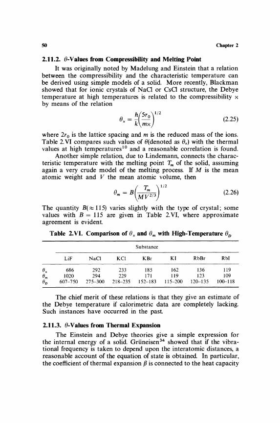
50 Chapter 2

2.11.2. O-Values from Compressibility and Melting Point

It was originally noted by Madelung and Einstein that a relation between the compressibility and the characteristic temperature can be derived using simple models of a solid. More recently, Blackman showed that for ionic crystals of NaG or esG structure, the Debye temperature at high temperatures is related to the compressibility x by means of the relation

Ox = ~(5ro)1/2 k mx

(2.25)

where 2ro is the lattice spacing and m is the reduced mass of the ions. Table 2.VI compares such values of O(denoted as Ox) with the thermal values at high temperatures 10 and a reasonable correlation is found.

Another simple relation, due to Lindemann, connects the charac­teristic temperature with the melting point Tm of the solid, assuming again a very crude model of the melting process. If M is the mean atomic weight and V the mean atomic volume, then

em = B(M~2/3) 1/2 (2.26)

The quantity B(:::::; 115) varies slightly with the type of crystal; some values with B = 115 are given in Table 2.VI, where approximate agreement is evident.

Table 2.VI. Comparison of ex and Om with High-Temperature eD

Substance

LiF NaCl KCl KBr KI RbBr RbI

ex 686 292 233 185 162 136 119 em 1020 294 229 171 119 123 109 eD 607-750 275-300 218-235 152-183 115-200 120-135 100-118

The chief merit of these relations is that they give an estimate of the Debye temperature if calorimetric data are completely lacking. Such instances have occurred in the past

2.11.3. O-Values from Thermal Expansion

The Einstein and Debye theories give a simple expression for the internal energy of a solid Griineisen34 showed that if the vibra­tional frequency is taken to depend upon the interatomic distances, a reasonable account of the equation of state is obtained In particular, the coefficient of thermal expansion P is connected to the heat capacity

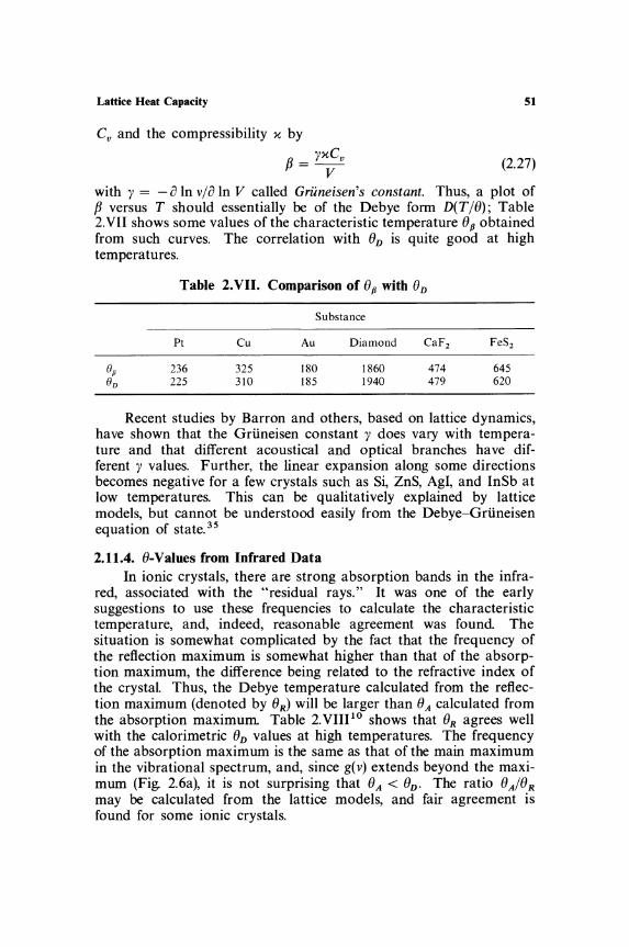
Lattice Heat Capacity

Cv and the compressibility x by

p = yxCv

V

51

(2.27)

with y = - a In v/a In V called Griineisen's constant. Thus, a plot of p versus T should essentially be of the Debye form D(T/()); Table 2.VII shows some values of the characteristic temperature (){J obtained from such curves. The correlation with ()D is quite good at high temperatures.

Table 2.VII. Comparison of (){J with ()D

Pt

236 225

Cu

325 310

Substance

Au

180 185

Diamond

1860 1940

CaF2

474 479

FeS2

645 620

Recent studies by Barron and others, based on lattice dynamics, have shown that the Griineisen constant y does vary with tempera­ture and that different acoustical and optical branches have dif­ferent y values. Further, the linear expansion along some directions becomes negative for a few crystals such as Si, ZnS, AgI, and InSb at low temperatures. This can be qualitatively explained by lattice models, but cannot be understood easily from the Debye-Griineisen equation of state. 35

2.11.4. ()-Values from Infrared Data In ionic crystals, there are strong absorption bands in the infra­

red, associated with the "residual rays." It was one of the early suggestions to use these frequencies to calculate the characteristic temperature, and, indeed, reasonable agreement was found The situation is somewhat complicated by the fact that the frequency of the reflection maximum is somewhat higher than that of the absorp­tion maximum, the difference being related to the refractive index of the crystaL Thus, the Debye temperature calculated from the reflec­tion maximum (denoted by ()R) will be larger than () A calculated from the absorption maximum Table 2.VIIIlo shows that ()R agrees well with the calorimetric ()D values at high temperatures. The frequency of the absorption maximum is the same as that of the main maximum in the vibrational spectrum, and, since g(v) extends beyond the maxi­mum (Fig. 2.6a), it is not surprising that () A < ()D. The ratio () A/()R

may be calculated from the lattice models, and fair agreement is found for some ionic crystals.

52 Chapter 2

Table 2. VOl. Debye Temperatures from Infrared Data

Substance

LiF NaG KCI KBr KI RbBr RbI

845 276 226 176 153 143 122 440 235 203 162 141 126 122

607-750 275-300 218-235 152-183 115-200 120-135 100-118

Actual infrared spectra show complicated structure, and some progress has been made in getting information about phonon­dispersion frequencies from the details of infrared and second-order Raman spectra. 36

2.11.5. O-Values from Electrical Resistivity

The temperature variation of the electrical resistivity of metals has been studied extensively, and a calculation of 0, denoted here as O(E.R.), on the basis of Bloch's theory of electrical conductivity was suggested by Grlineisen He showed that the ratio of the specific resistance (T to its value (Too at high temperatures is of the form

(2.28)

However, as pointed out by Blackman,lO O(E.R.) involves only longi­tudinal phonons in the theory, hence, it should differ considerably from 0D. In practice, there is a very surprising correlation between O(E.R.) and OD for many metals, as shown by Table 2.1X. At present, there is no satisfactory explanation of the agreement!

Table 2.IX. Correlation of 0 (E.R.) with OD

8(E.R.)

°D

Li Cu Ag

363 333 203 340-430 310-330 212

Metal

Au Pb

175 86 168-186 82-88

2.11.6. Scattering of X-Rays, y-Rays, and Neutrons

AI

395 385

w

333 305-357

The vibrations of atoms in a solid affect the reflection of X-rays and other radiations of similar wavelength A. from the crystal lattices. There are two principal effects--a reduction of the intensity of Bragg

Lattice Heat Capacity

Table 2.X. Values of () (X.R.), () (EI.), and ()D at 3000 K

8(X.R.) 8D 8(El.)

Al

379 396 406

Cu

307 310 331

Pb

80 93 91

Substance

Fe

393 425 464

Diamond

1491 1850 2242

Si

593 640 647

53

reflections (by the so-called Debye-Waller factor) and a diffuse scattering of radiation in the non-Bragg directions. The intensity of the Bragg reflection at an angle ¢ from a monatomic solid depends upon the temperature T in the form I = 10 exp( - 2M), where M = 8n2 u2 ~sirt~d?12:2. The mean square amplitude u2 perpendicular to---ulefeflecting plane may be calculated if a model of the lattice vibration is assumed. For a Debye solid at high temperatures,

M = (2kT sin ¢)2 3h2

mI. k 2 ()2

and thus from the Debye-Waller factor, the characteristic tempera­ture, denoted as ()(X.R.) in Table 2.X, may be calculated. In the lattice case, the term 3h 2/k 2 ()2 is replaced by S g(v)v- 2 dv/S g(v) dv, so that ()(X.R.) is in general different from ()D' Some representative values30

of ()(X.R.), ()(EL), and ()D at 3()()OK are given in Table 2X In general, ()(X.R.) is less than ()(El.) or ()D; this is roughly what is expected from the lattice theory. Herbstein30 has given a detailed discussion of the thermal effects in X-ray, Mossbauer, and neutron scattering, which may be referred to for further details.

The use of diffuse X-ray reflections and inelastic neutron­scattering in providing information about phonon-dispersion rela­tions has already been mentioned. 20-22,37

REFERENCES

I. A. Eucken, Handbuch der experimental Physik, VIII (I) (1929), chapter 5. 2. A. J. Rutgers, Physical Chemistry, Interscience, New York, 1954, chapters II

and 33. 3. J. C. Slater, Introduction to Chemical Physics, McGraw-Hill, New York, 1939,

chapters 3 and 4. 4. Landolt-Bornstein physikalish chemische Tabellen, Springer-Verlag, Berlin, ed. 5,

suppl. I, p.702 (1927); ed. 6, Vol. 2, Part 4, p.736 (1961). 5. J. Sherman and R. B. Ewell, J. Phys. Chem. 46, 641 (1942). D. R. Stull and

F. D. Mayfield, Ind. Eng. Chem. 35, 639 (1943). H. Zeise, Thermodynamik, Vol. 3, Hirzel, Leipzig, 1954. W. C. Overton and J. H. Hancock, Tables of Einstein Functions, U.S. Naval Res. Lab. Rep!. No. 5502 (1960). J. Hilsenrath and G. G. Ziegler, Tables of Einstein Functions, Nat. Bur. Std. Monograph No. 49 (1962).

54 Chapter 2

6. 1. de Launay, Solid State Phys. 2,219 (1956). 7. R. F. S. Hearmon, Introduction to Applied Anisotropic Elasticity, Oxford University

Press, Oxford, 1961. 8. M.l. P. Musgrave, Rept. Progr. Phys. 22, 74 (1959); Progr. Solid Mech. 2, 63 (1961). 9. H. Weyl, Math. Ann. 71, 441 (191\). R. D. Courant, Math. Ztschr. 7, 14 (1920).

W. Ledermann, Proc. Roy. Soc. (London), Ser. A. 182, 362 (1944). R. E. Peierls, Proc. Nat. Inst. Sci. India 20A, 121 (1954).

10. M. Blackman, Handhuch der Physik, VII (1),325 (1955). I\, 1. A. Beattie, J. Math. Phys. (MIn, 6, I (1926). 12. G. F. Newell, J. Chern. Phys. 23, 2431 (\955). L. S. Kothari and V. K. Tewary.

J. Chern. Phys. 38,417 (\963). B. 1. C. van der Hoeven and P. H. Keesom, Phys. Rev. 130, 1318 (1963).

13. E. Schrodinger, Handbuch der Physik, X, 275 (1926). 14. D. Bijl, Progr. Low Temp. Phys. 2, 395 (\957). 15. 1. D. Filby and D. L. Martin, Proc. Roy. Soc. (London), Ser. A 276, 187 (1963). 16. W. T. Berg and 1. A. Morrison, Proc. Roy. Soc. (London), Ser. A 242,467 (1957). 17. M. Blackman, Rept. Pro!?r. Phys. 8, II (1941). 18. L. Brillouin, Wave Propagation in Periodic Structures, Dover, New York, 1954. 19. G. H. Wannier, Elements of Solid State Theory, Cambridge University Press.

Cambridge, 1959, chapter 3. 20. L. S. Kothari and K. Singwi, Solid State Phys. 8, 109 (1959). 21. A. A. Maradudin, E. W. Montroll, and G. H. Weiss, Theory of Lattice Dynamics

in the Harmonic Approximation (suppl. 4 to Solid State Physics), Academic Press. New York, 1963.

22. W. Cochran, Rept. Progr. Phys. 26, I (1963). 23. A. E. Dixon, A. D. B. Woods, and B. N. Brockhouse, Proc. Phys. Soc. (London)

81,973 (1963). G. Gilat and G. Dolling, Phys. Letters 8, 304 (1964). 24. B. Dayal and S. P. Singh, Proc. Phys. Soc. (London) 76, 777 (1960). B. Dayal

and B. B. Tripathi, Proc. Phys. Soc. (London) 77, 303 (I96\). 25. G. Leibfried, Handbuch der Physik, VII (I), 104 (1955). 26. R. G. Chambers, Proc. Phys. Soc. (London) 78, 941 (1961). 27. S. O. Lundqvist, V. Lundstrom, E. Tenerz, and 1. Waller, Ark. Fysik 15,193 (1959). 28. C. B. Walker, Phys. Rev. 103, 547 (1956). 29. G. Liebfried and W. Ludwig, Solid State Phys. 12, 275 (1961). T. H. K. Barron

and M. L. Klein, Phys. Rev. 127, 1997 (1962). R. A. Cowley, Advan. Phys. 12. 421 (1963).

30. F. H. Herbstein, Advan. Phys. 10,313 (1961). 31. 1. R. Partington, Advanced Treatise on Physical Chemistry, Vol. 3, Longmans­

Green, London, 1952, section 9N. 32. G. A. Alers and 1. R. Neighbours, Rev. Mod. Phys. 31, 675 (1959). 1. L. Feldman,

Proc. Phys. Soc. (London) 84, 361 (\964). 33. O. L. Anderson, J. Phys. Chern. Solids 12, 41 (\959). P. Flubacher, A. 1. Lead­

better, 1. A. Morrison, and B. P. Stoicheff, J. Phys. Chern. Solids 12, 53 (1959). H. B. Rosenstock, J. Phys. Chern. Solids 23, 659 (1962).

34. E. Griineisen, Handbuch der Physik X, I (1926). 1. K. Roberts, and A. R. Miller, Heat and Thermodynamics, Blackie, London, 1960, chapter 22.

35. C. Domb in Proceedings of the Eighth International Conference on Low Temperature Physics (London, 1962, R. O. Davies, editor), Butterworth, London, 1963, p.385. J. G. Collins and G. K. White, Progr. Low Temp. Phys. 4, 450 (1964).

36. S. S. Mitra, Solid State Phys. 13, I (1962). F. A. lohnson and R. Loudon, Proc. Roy. Soc. (London), Ser. A 281,274 (1964).

37. W. A. Wooster, Diffuse X-Ray Reflectionsfrom Crystals, Clarendon, Oxford, 1962.

Chapter 3

Electronic Specific Heat

3.1. SPECIFIC HEAT OF METALS

Metals are characterized by their high electrical and thermal conductivities at ordinary temperatures. When the discrete nature of electric charges became clear, by about 1900, it was also realized that freely moving electrons were the charge carriers in metals. Drude, Lorentz, and others applied the methods used in the kinetic theory of gases to explain how these electrons were responsible for the observed high thermal and electrical conductivities. 1

In spite of the success of the free-electron gas model, the classical theory had a fundamental inconsistency. If the electrons are con­sidered as small particles freely moving through the crystal lattice, the equipartition law attributes to each electron an internal energy -ikT, associated with the three translational degrees of freedom. Therefore, the electrons should contribute -iR per mole to the specific heat. A monovalent metal such as copper should thus have C v ~ 9 caljmole·degK, 3R from the lattice and -iR from the conduction elec­trons. The experimental value of 6 caljmole·degK is entirely accounted for by the lattice contribution. The same is true for almost all metals at room temperature, as can be seen from the values given in Table 2.1. The model of an electron gas in a metal explained the transport properties reasonably well, but the caloric behavior was in complete disagreement with the equipartition theorem.

It was only in 1928, after Sommerfeld's application of quantum statistics to free electrons in a metal, that the reason for the small electronic specific heat became evident. Even as Bose-Einstein statistics applied to phonons brings about a reduction of lattice heat capacity at low temperatures, the Fermi-Dirac statistics obeyed by electrons makes the electronic specific heat comparatively small at room temperatures. It became clear that the electronic contribu­tion could be observed only at very low temperatures, in the liquid-

55

56 Chapter 3

helium range, and the first experiments to study electronic specific heats in detail were performed by Keesom and coworkers in the early 1930's.

3.2. QUANTUM STATISTICS OF AN ELECTRON GAS

It is a fundamental feature of quantum statistics, as explained in several texts,1.2 that because of the Pauli exclusion principle and because the various electrons are indistinguishable from one another, Fermi-Dirac statistics should be applied to electronic systems. Ac­cording to F-D statistics, the probable number Nk of particles in energy state ek is

N - gk

k - exp[(ek - eF)/kT] + (3.1)

where gk is the number of levels with energy ek and the parameter eF

(the Fermi energy) is so chosen that the total number of particles is equal to N. The energy levels are often so closely spaced that it is convenient to define the density of states 91(e) de as the number of energy states per unit volume between e and e + de.

For a F-D system, marked deviations from classical Maxwell­Boltzmann behavior occur when the temperatures are lower than the Fermi temperature TF = eF/k, which in ordinary metals is of the order of 105 °K. The shape of the F-D function

1 f(f,) = --~-----=-== . 1 + exp[(e - f,F)/kT]

(3.2)

is shown in Fig. 3.1 for various temperatures. As T ---> 0, !(t.) equals unity for any energy less than eF and then abruptly drops to zero for t. > t.F' In other words, all the energy states below eF are fully occupied, while all states above t.F are empty. At a finite temperature T, some of the particles within a distance of approximately kT of t.F have enough thermal energy to become excited to higher energy states, as shown in Fig. 3.1. However, at T/TF ~ 0.01, the distribution has changed little from the behavior at T ~ 0; it is only for T ~ TF that the familiar Boltzmann tail of the distribution makes its appearance.

The magnitude of the Fermi temperature TF , which is obviously fundamental to an understanding of the behavior of an electron gas, can be easily calculated as follows. In Chapter 2, it was shown that for free particles in a volume V, the number of allowed energy states between momenta p and p + dp is

4nV n(p) dp = IJ3 p2 dp (2.18)

Electronic Specific Heat

1.0

0.8

0.6

!(c)

0.4

0.2

o

". ' . "\ f- T' OJ . • . : ~ T T(IOO

". . T • ~F/ l0 .

. ,

. "

,

• . I I . . , .....

o 0.2 0.4 0.6 0.8 1.0 1.2 1. 4

cl eF

Fig. 3.1. Shape of the F-D function [equation (3.2)] at various temperatures.

57

If m is the mass of an electron, the number of allowed states can be written in terms of the energy S = p2 j2m as

V V 91(s) ds = 2re(2m)3 /2 h3 s1/2 ds (3.3)

At OaK, all states below EF are occupied, and, further, each state can be filled by two electrons of opposite spins. So the total number of states is

N V _ = !re(2m)3/2 _ S3/2 2 3 h3 F

or

EF = _1_(iNh3 )2/3 2m reV

(3.4)

This formula is valid for a gas of free electrons; nevertheless, suppose a value typical of a metal N jV :::::: 1023 jcm 3 is substituted. Then

The Fermi energy SF of a gas of electrons with metallic densities is two or three orders of magnitude greater than the thermal energy of

58 Chapter 3

approximately kT at room temperatures. The electron gas is said to be highly degenerate under such conditions.

It is very surprising that in spite of such high energy content the specific heat of the electron gas is quite small. This comes about because the internal energy changes very little at ordinary tempera­tures. To a first approximation, a fraction ( '" kT /f-F) of the number of electrons is excited at a temperature T into higher energy states (see Fig. 3.5). Each electron gains an energy of about kT, and so the increase in energy per mole is bE '" RT(kT/CF)' The heat capacity is therefore approximately 2R(T /TF) per mole. Since TF ~ 104 to lOsoK, the electronic heat capacity is about 1O- 2R at room tempera­ture. This is only 1 % of the lattice heat capacity at ordinary tempera­tures. However, at very low temperatures, the lattice heat capacity, falling off as T 3, decreases much faster and becomes comparable to the electronic term, which decreases only linearly with T. These qualitative conclusions are in excellent agreement with experimental results.

3.3. SPECIFIC HEAT OF ELECTRONS IN METALS

The model of a free-electron gas, although forming an elementary introduction to the behavior of electronic systems, is unnecessarily crude when applied to actual metals. The electrons in the inner shells of an atom are tightly bound to the nucleus; only the electrons in the outer unfilled shells have any chance to wander through the metal. Their movement is subject to the three-dimensional periodic potential field associated with the atoms of the lattice. Under these conditions, the energy levels, instead of being a continuous function p2/2m of the momentum, become grouped into energy bands. 3 In each band, the energy is a continuous function of momentum, but the bands them­selves are separated by gaps in which there are no energy levels (Fig. 3.2). Ordinarily, the first band is completely filled (valence band), while the second band is only partially filled (conduction band). Electrons in any unfilled band can move under applied electric fields and thereby transport quantities of electricity or heat. In an ordinary dielectric, the valence band is just full; in the absence of any free carriers, the material behaves as an insulator. In three momentum dimensions, the surfaces of constant energy have complicated shapes because the energy-momentum relationship depends upon the crystallographic directions. The shape of the Fermi surface, i.e., the surface in the momentum space enclosing the occupied states of electrons in a metal, can in some cases be determined from other electronic properties of the meta1.4 •S

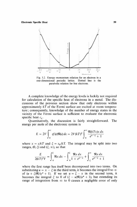
Electronic Specific Heat

,. , ,

'\' . · . · . · . · . · ,.

N : '

- - - -o 0

h o

::

./': · . · . · . · . · . ./ ( :

· . · . · . · . · . ;;- .

o 2hn

o Momt' I"I 'um

3h r o

Fig. 3.2. Energy-momentum relation for an electron in a one-dimensional periodic lattice. Dotted line is the

parabolic relation for free electrons.

59

A complete knowledge of the energy levels is luckily not required for calculation of the specific heat of electrons in a metal. The dis­cussions of the previous section show that only electrons within approximately kT of the Fermi surface are excited at room tempera­ture; consequently, knowledge of the number of energy states in the vicinity of the Fermi surface is sufficient to evaluate the electronic specific heat Ce .

Quantitatively, the discussion is fairly straightforward. The energy per mole of the electronic system is

Jw f ro 91(kTx)x dx E = 2 V Ef(E)91(E) dE = 2 V(kT)2 -x--~~ --

o 0 e + 1

where x = E/kT and ~ = EF/kT. The integral may be split into two ranges, (0, ~) and (~, (0), so that

E f~ f~ 91x dx f ro 91x dx 2(k T)2 V = 0 91x dx - 0 1 + e~ x + ~ eX ~ + 1

where the first range has itself been decomposed into two terms. On substituting u = x - ~ in the third term, it becomes the integral 0 to 00

of (u + ~)91/(eU + 1). If we set u = ~ - x in the second term, it becomes the integral ~ to 0 of (~ - u)91/(eU + 1), but extending its range of integration from 00 to 0 causes a negligible error of only

60 Chapter 3

e-~. Therefore, to the lowest-order terms,

E = 2VJ~ 91(t:}t:dt: + 4V(kT)291(t:FlXl ~ dU.

o Joe + The first term on the right is the internal energy at OaK, while the integral 0 to 00 of u/(e" + 1} may be transformed into the series

which has the value n2 /12. So the energy per mole is

E = Eo + jn:2V(kT)291(t:F)

The molar heat capacity of the electronic system is

Ce = tn:2k2V91(t:F)T = 1'T

(3.5)

(3.6)

The electronic specific heat is determined only by the density of states at the Fermi surface 91(t:F}, as was expected earlier. To make a numerical estimate of Ce , assume the metallic electrons to be free. From equations (3.3) and (3.4), the molar density of states is

(3.7)

Consequently,

_ 4n3mP(3NV2)1/3 Ce - 3h2 -n- T

= 3.26 x 10- 5V2/3n~/3T cal/mole·deg (3.8)

= 1.36 x 1O-4V2j3n~/3T l/mole·deg

where n~ is the number of free electrons per atom. For a typical metal, say, copper at room temperature, V - 7 cm3 /mole, n~ = 1, T - 300oK, and so Ce ~ 0.04 caljmole·deg. This is less than 1 % of the lattice heat capacity of 6 caljmole·deg at the same temperature. Therefore, the electronic specific heat is not normally detected in room-tempera­ture measurements. This explanation was indeed one of the great triumphs of Sommerfeld's application of quantum statistics to the theory of metals.

The above linear variation of electronic specific heat is valid only at low temperatures (T ~ TF). At higher temperatures, the calculations are involved6 ; the full variation is shown in Fig. 3.3. For T ~ TF ,

the limiting value is iR, which is the classical equipartition value for a gas of structureless mass points (Section 6.2).

Electronic Specific Heat

I.Sr--I-=I::::::::::lF=~

1.0+-----,f---+-----t----1------t

o.s ...... -I----+----4-----1f------I

o~------.. ----.. ----__ ~----... 0.5 1.0

T/TF

1.5 2.0

Fig. 3.3. Temperature variation of the heat capacity of an electron gas.

3.4. ELECTRONIC SPECIFIC HEAT AT LOW TEMPERATURES

61

Although at room temperature the electronic contribution to the heat capacity of a metal is insignificant compared to the lattice contribution, the situation is quite different at low temperatures. Ce decreases linearly with T, whereas C g , as seen in the previous chapter, is proportional to T3 at low temperatures. Therefore, at some temperature, the two terms become equal; at still lower tem­peratures, C e is larger than Cg (Fig. 3.4). For instance, copper at about 4°K has Cv '" 6 x 1O- 3J/mole'degK, which is equally shared between electronic and lattice contributions. Above about 4°K, the lattice part rapidly dominates the specific heat, while below that temperature the electronic part remains significant. In general, at liquid-helium temperature, both terms are of comparable magnitude and the observed specific heat is of the form

C = Cg + Ce = f3T 3 + yT (3.9)

A plot of CIT against T2 should therefore be a straight line, and, indeed, a typical example was given in Fig. 1.1 b to illustrate how well the relation (3.9) is obeyed, if the T3-region of the lattice specific heat has been reached. Such a plot permits determination of both f3 and y. From equation (2.20) it is evident that f3 = 12n4RISlJ3 • The value of the Oebye temperature at very low temperatures (lJo) and the coefficient y of the electronic specific heat for a number of metals are given in Table 3.1. The values refer to materials of the highest-

u

~ "-e u

62 Chapter 3

l0 r--------r--------~------~--------~----~~------__,

8

i /

/

I .I

I i

i

---

./

I i

I

l .I

I

---

O~~--~~~~~~~------~------~~------~~----~3.0

T(dog K)

Fig. 3.4. Typical low-temperature heat capacity of a metal, sodium: 1 - 0 - 0- 0 __

observed C p; - . - . - . lattice term; - - - - electronic term.

available purity. Impurities in the metal affect the specific heat slightly, and in some cases anomalous values have been obtained.s Besides the possible changes in 91(cF) due to the impurities, dilute magnetic contaminations may in some cases give a term linear in T; careful analysis is needed to unravel the various effects (Section 3.6).

The free-electron gas model is obviously oversimplified. Never­theless, equation (3.8) gives a value ofy of the right order of magnitude. For example, in sodium, there is one electron in the outer unfilled shell, which is almost free to move; according to (3.8), y should have a value of 11 x 10- 4 J/mole·deg2 . Similarly, copper, which also has one outer electron, should have y = 5.4 in the same units. The experimental values are Na = 13.7 and eu = 7.0. A simple way of illustrating the difference between theory and experiment is to intro­duce an "effective mass" m* which takes into account the partial binding, namely, the fact that the electrons are not completely free but are only loosely bound to the metallic ions. The electron mass m in equation (3.8) is now replaced by m*, so that

Yexp m* (3.10)

Ytheor m

Electronic Specific Heat 63

Table 3.1. Representative Values of 80 (in deg K) and y (in 10- 4 J jmole·deg2)

Metal 80 }' Metal 80 y

Ag 225 6.09 Na 158 13.7 Al 426 13.6 Nb 250 88.2 Au 164 7.0 Ni 440 72.8 Ba 110 27.0 Os 500 23.5 Be 1160 2.22 Pb 108 33.6 Ca 229 27.3 Pd 299 99 Cd 209 6.9 Pt 221 66.3 Co 443 47.5 Rb 55 24.1 Cr 585 15.5 Re 450 24.5 Cs 39 32.0 Rh 478 48.9 Cu 348 7.0 Ru 600 33.5 Fe 464 50.2 Sn (white) 195 17.5 Ga 324 6.0 Sr 147 36.5 Hf 261 26.4 Ta 245 58.5 Hg 72 18.6 Th 170 46.8 In 109 18.4 Ti 430 35.5 Ir 420 31.4 TI 90 15.2 K 91 20.8 U 200 109 Li 369 17.5 V 380 92 Mg 342 13.7 W 405 12.1 Mn 450 180 Zn 310 6.27 Mo 470 21.1 Zr 310 30.3

Thus, m*jm has a value of about 1.2 for sodium and about 1.3 for copper. For other metals, the appropriate valence of the atom is used to represent n., the number of electrons per atom. In this manner, m*jm-values have been calculated and tabulated in several reviews. 8 - 10

Although the value of m* jm suggests the degree of departure from the electron gas model, the quantity has only a limited significance. In metals, the bands usually overlap, and the details of the band structure are quite complicated.4 ,5 The idea of an effective mass, which can be easily introduced in the case of a single band, is not appropriate under such conditions. Moreover, in cyclotron resonance, the de Haas-van Alphen effect, and other phenomena which reveal the properties of Fermi surfaces more directly, different "effective masses" are introduced, leading to some confusion in comparing the values of m* jm for any particular substance. The situation corres­ponds to the confusion concerning the indiscriminate use of the Debye 8 to characterize different physical properties, as mentioned in Chapter 2. Therefore, it appears best to express the experimental results in terms of y, as done in Table 3.1.

64 Chapter 3

Electrons, because of their electric charge, exert Coulomb forces upon one another; these forces are of long range, falling off as 1jr2. It would appear that the use of a perfect-gas model is inconsistent with the existence of such long-range interactions. In fact, early approximate calculations showed that the specific heat would be about ten times smaller than the Sommerfeld value and would also have a different temperature dependence, thereby destroying even the qualitative agreement between equation (3.8) and experiments. More recently, the exchange and correlation effects of the Coulomb interaction have been analyzed in detail, using the mathematical techniques developed for handling many-body problems. It turns out that each electron is shielded, as it were, by the nearby polarization cloud of the electron gas. The interaction potential V(r) becomes screened, V(r) - e2r- 1 exp( - ;.r), so that it becomes a short-range force, which is compatible with the perfect-gas model of the electrons. The collective motion of the electron clouds is then described in terms of what are called plasma modes, which have too high a frequ­ency to be involved in specific-heat studies. The details of these calculations are left to suitable reviews. 11

Another aspect of the electronic specific heats of metals, which cannot be treated here, is the interaction between electrons and phonons. In writing equation (3.9), it is implictly assumed that electronic motions are independent of lattice vibrations, so that the two terms are simply added together. It is, however, obvious that the vibrations of an atom will influence the motion of electrons in its neighborhood; conversely, the presence of the electron cloud will affect the lattice vibrations. For many metals, the effect is very small, 12

but two exceptional situations occur. In some cases, the electron­phonon interaction results in the phenomenon of superconductivity, as originally suggested by Frohlich in 1950. The properties of super­conductors are so striking that they are discussed separately in Sections 3.8 to 3.10. In a few special cases, electron-phonon inter­actions result in small anomalies, known as Kohn anomalies, in the lattice w-q dispersion relations. 13

3.5. SPECIFIC HEAT AND BAND STRUCTURE OF METALS

A discussion of the values of y for all metals is clearly to be left to special reviews on the subject. 8 ,9,lO,14 Only a few typical metals are considered here, in order to illustrate the special factors involved in a study of electronic specific heats.

The alkali metals lithium, sodium, potassium, rubidium, and cesium, have one "free" electron in the outer shells. The inner closed shells are tightly bound to the nucleus, and consequently we may

Electronic Specific Heat 65

assume that there are N electrons per gram-atom. The number of states in the valence band is N, which can be filled by 2N electrons. The first Brillouin zone is thus only half-filled, and the free-electron model may be expected to be useful. This model gives

V91(E)dE = 2n(2m)3/2Vh- 3E1/2dE

as shown in Fig. 3.5. Nevertheless, the observed values of yare not in good agreement with equation (3.8). Apart from sodium, mentioned earlier, m*/m has a value 15 of 1.25 (K), 1.26 (Rb), and 1.43 (Cs), showing that even in such simple cases the free-electron model is not adequate. Calculations using details of the band structure, electron-phonon and electron-electron couplings, account reasonably well for the experimental values of m* /m.

The noble metals, copper, silver, and gold, are also monovalent and have their first Brillouin zones half-empty. The values of m*/m, 1.36 (Cu), 1.05 (A g), and 1.16 (Au), differ appreciably from unity, which at this stage is not surprising. The Fermi surface of copper has been investigated by several methods; its shape is shown in Fig. 3.6. In a free-electron gas model, it will be a sphere, whereas in copper it is actually pulled out and touches the zone boundaries along the < III > directions. Detailed calculations based on such Fermi sur­faces do fit in well with the experiments. The specific-heat data are not very useful for finding the shape of the Fermi surface, because the electronic term measures merely an averaged density of states at

-kT

Energy f

Fig. 3.5. Energy distribution in an electron gas. Full line is the number of electrons at a finite temperature, broken

line is that at absolute zero.

66 Chapter 3

Fig. 3.6. Fermi surface of copper.

the Fermi surface. If the shape of the Fermi surface is known from other studies,4.5 }' can be used as a final check.

The divalent metals, beryllium, magnesium, calcium, zinc, cadmium, etc., have hexagonal crystal structure. With two "free" electrons per atom, the Brillouin zones should be exactly filled and the substances should be insulators. As a matter of fact, the first and second bands overlap to some extent, which accounts for the electrical conductivity of the metals. The Fermi surface intersects the zone boundary and has a complex shape. The theoretical calculation of 9l(8F ) is a matter of considerable labor. The only simple statement that can be made 16 is that 9l(8F ) varies rapidly when the axial ratio cia of the hexagonal lattice is small and is nearly constant when the ratio is large. Beryllium (cia = 1.57, )' = 2.22 X 10- 4 J/mole'deg2)

and magnesium (cia = 1.62, )' = 13.7) belong to the first set, while zinc (ci a = 1.86, )' = 6.3) and cadmium (cia = 1.89, )' = 6.3) are examples of the second case.

The transition metals form another interesting example of the effect of electronic structure, as was first pointed out by Mott. An inspection of the values of}' for the first group of metals (Table 3.11) shows that the electronic specific heats are unusually large. In

Electronic Specific Heat 67

Table 3.D. Values of y for the First Group of Transition Metals

Metal

Ti v Cr Mn Fe Co Ni

y X 104 J/mole'deg2 35.5 92 15.5 180 50.2 47.5 72.8

isolated atoms of these metals, the filled 4s-subshell, containing two electrons, has as usual a lower energy than the partially filled 3d­states (chromium has only one electron in the 4s-level, and the value of y is also exceptional). When the atoms are brought together to form a metal, the wave functions of the states overlap, which produces a characteristic broadening of the energy levels. The wa ve functions for the 4s-states are more extended than those of the 3d-states. Consequently, the 4s-band is broader and covers a much wider range than does the 3d-band. This occurs to such an extent that some states in the 4s-band have higher energies in the metal than those of the 3d-band, as schematically represented in Fig. 3.7a. Moreover, the 4s-band contains only two states per atom, or 2N states per mole of the metal. It has a large energy spread, and so its density of states is low. The 3d-band contributes 10 N states to the metal; since its energy spread is small, the density of states is large. The resultant density of states as shown in Fig. 3.7b, has a sharp maximum. The Fermi levels lie in this region, and hence Ce is unusually large for

t' ... \

4Sr-_~

Melol

10 1 (b )

Fig. 3.7. (a) Broadening of 4s- and 3d-bands in a metal due to overlap. (b) Density of states for 4s- and 3d-bands. Dotted line is the resultant density of states.

68 Chapter 3

these metals. For a quantitative analysis, the details of the band structure must be worked out. 14

The metals of the second and third transition groups also have large values of y, for similar reasons. Furthermore, the unfilled shells give rise to magnetic interactions among the atoms. The resulting para-, ferro-, and antiferromagnetic behavior produces interesting effects in specific heats which will be discussed in the next chapter. The ions of rare-earth metals also have unfilled shells. But the coupling among the ions is weak, and various magnetic and other transitions occur below room temperature. Rare-earth specific heats are dis­cussed in Chapter 7, Section 6.

3.6. SPECIFIC HEAT OF ALLOYS

When two metals are alloyed, there is in general a change in the lattice structure. A structural change alters not only the lattice specific heat directly, as is clear from Chapter 2, but also the electronic term, through the influence of the lattice structure upon the energy­band scheme. In such general cases, no simple rule can be given. It is only in special circumstances that simple correlations exist. One such instance is that of a binary alloy, for instance, f3-brass (CuZn), which exhibits an order-disorder transition, but this is more appropriately taken up in Chapter 7.

In several dilute alloys, especially of elements of near atomic number and similar atomic radii, the elements go into solid solution without any appreciable change of crystal structure. The observed variation of specific heats may then be attributed to variation in 91(£), and some information may be obtained about the shape of the den­sity-of-states curve. The simplest hypothesis, the rigid-band model, is to assume that in the process of alloying, the band structure re­mains unchanged and only the number of available electrons is altered. The value of 91(£F) at the new Fermi level determines the electronic specific heat of the alloy [equation (3.6)]; depending upon the slope of the 91(£) curve at the band edge, the y of the alloy will be larger or smaller than that of the pure metal. In this manner, the electronic specific heat may be correlated with the shape of the energy-band scheme.

As an instance, palladium can be freely alloyed with its neighbor­ing elements silver and rhodium. The y-values of these alloys17 are shown in Fig. 3.8a. In the rigid-band model, the addition of silver to palladium gives an extra electron per atom of silver; these extra electrons fill the band to a higher energy level. The alloying with rhodium gives one hole per Rh atom, and so the Fermi level occurs at a lower value of energy. Thus, the density-of-states curve (Fig. 3.8b)

12 l'

10

v_

8 ,. ,

~

"0

~ 1

6 v_

E

~- o

Rh

I I

-' • • •

• •

• • •

1 • •

1 50

Pd

Com

pos

ition

(a

tom

ic%

)

(0)

I --

--,

---,

--,

----

,

• ••

• ... 50

Ae

5 .-2.

0 c .£ ~ '0

c .~ ~ E

E

c ~ l: C

:;;

1.0

(;

~

~ ~ o

o

; ;

f J / :1. I I I I I 1-:- Rh

I I I I I I I I , : \

I I ~

I I Pd

4

, , ,

En

erg

y (e

V)

(b)

: 5

All

6

[ g ;:j'

(fJ 1 ~ :c .. a

Fig,

3.

8. (

a) E

lect

roni

c sp

ecif

ic-h

eat

coef

fici

ents

for

pa

llad

ium

-sil

ver

and

pall

adiu

m-r

hodi

um a

lloy

s.

(b)

Den

sity

of

stat

es p

er

atom

, rh

odiu

m-p

alla

dium

-sil

ver,

for

one

dir

ecti

on o

f sp

in.'

7 ~

70 Chapter 3

may be drawn at once. For reasons set forth in the previous section, the 4d-band in a metal of the second transition group should be sharply peaked, while the 5s-band should be comparatively flat. There is indeed a striking similarity between Figs. 3.7b and 3.8b. Theo­retical calculations of the band structures are in good agreement with Fig. 3.8b, but the details of such studies 14.17 cannot be included here.

Dilute alloys of transition elements show several peculiarities which have not yet been clarified. ls As an example, if small amounts of manganese are added to copper, the specific heat in the liquid­helium range is abnormally increased. 19 The heat capacity is linear in T at very low temperatures and is roughly independent of the manganese concentration c. At higher temperatures, it falls rapidly to the pure-metal value. The temperature at which this decrease occurs is proportional to c, so that the entropy associated with the extra heat capacity ~C is proportional to the number of manganese ions. Figure 3.9 shows how at low concentrations of manganese, the y­values are abnormally high and independent of c, while at high concentrations normal behavior is approached. Similar results are obtained in dilute alloys of iron in copper, also. In some alloy systems, the specific heat shows a definite maximum before the ~C rx T region is reached. These deviations are accompanied by corresponding anomalies in other properties such as magnetic susceptibility and electrical conductivity.

The theoretical picture of dilute alloys of transition elements is 15

12 ...,

""\ \

6 " ~ ~ ~ ... ...

~ ... ... --"'oC

20 40 60 80 100

Weight "~o of (.opper in manganese

Fig. 3.9. Electronic specific-heat coefficients of copper-manganese alloys.!O The broken line shows the expected behavior of dilute manganese in copper.

Electronic Specific Heat 71

still under debate, although considerable progress has been made by Friedel and others 18 regarding the formation of localized moments. It was Overhauser2o who suggested an explanation for the observed specific-heat behavior; subsequent developments have been due to Marshall and others.20 They all involve some form of magnetic ordering and the extra specific heat L\C arises when a number of spins are located in regions of near-zero magnetic field. The near-zero field regions may arise from the stationary spin-density waves, from the large separation between the magnetic ions, or from the approxi­mate cancellation of the exchange interactions of opposite sign. Although magnetic interactions are taken up in Chapter 4 only, the effects may be calculated in a crude manner as follows. At a tempera­ture T and in a field H, a magnetic dipole J1 has an average energy [see equation (4.15)] -J1H tanh (J1H/kT). In an alloy, the local magnetic field varies from site to site, and, if f(H) is the probability of having a field H at the site of J1, the internal energy is

E ~ -tNc f:", f(H)J1H tanh (~~) dH

where c is the concentration of manganese ions and Nc their total number. Most of the ions will be rigidly aligned because they are in effective fields much larger than kT/J1 at low temperatures. So they do not contribute to the heat capacity. Only the ions situated in near-zero fields J1IHI ;S kT will be able to change their orientations and hence give an excess specific heat L\C. Thus

L\C - tNCf(O)f~oo (~2~2) sech2 (~~)dH In a fully aligned perfect lattice, the magnetic field at an ion has a definite value, though thermal fluctuations smear out the field to some extent. In an alloy, the field is completely smeared out and has a wide range of values. Under these conditions, the probability of finding zero field at a site is proportional to l/<H), where <H) is the mean field at an ion. Since the interactions are mainly dipolar, (H) will be proportional to R - 3 (R is the mean distance between Mn ions) and hence to c, the concentration of Mn ions. Therefore, with suitable constants A, Af,

L\C ~ AT roo x2 sech2x dx = AfT

At low temperatures, the specific heat is proportional to T and independent of the manganese concentration; these are the two important experimental observations. Detailed calculations20 show

72 Chapter 3

that at higher temperatures LlC falls off as T- 2 ; the temperature at which this occurs is proportional to c, which again agrees with the observations. The subject is of current interest, and the overall picture is just emerging.

3.7. SPECIFIC HEAT OF SEMICONDUCTORS

A pure semiconductor differs from a metal in that, at absolute zero, the first Brillouin zone is completely filled by electrons and the next zone is completely empty. There is no overlap between the bands (Fig. 3.10a). The energy gap is small, however, and at ordinary temperatures some electrons are excited from the valence band to the conduction band (Fig. 3.1Ob.) The material is now electrically conducting and becomes more so when the temperature is raised, unlike pure metals, which become less conducting when T is increased. In practical applications, materials with controlled amounts of suitable impurities (dope) are of tremendous importance. The impurity atoms introduce extra energy levels into what was earlier the forbidden energy gap. The presence of such levels alters the electrical properties profoundly, because electrical conduction can take place without thermal activation of electrons across the energy gap. The special properties of semiconductors are far too numerous to chronicle here; for an introduction, one may refer to the elementary texts mentioned earlier. 3

In all types of semiconductors, whether pure or slightly doped, the density of excited current carriers decreases rapidly as the tempera­ture is reduced. Therefore, at low temperatures only the lattice specific heat is observed for most semiconductors.21 Germanium, silicon, and indium antimonide are among the most intensely studied

Conduction bond , , " Free electrons

Gap

I __ Holes

••••••••••••• c •• dbb •••• ••• Valence ••• • •••••••••• ••• band •••• ••••••••••

ToO T>O

Conduction bond

Impurity levels

/

---------Valence band

(a) (b) (c)

Fig. 3.10. Simplified energy-level diagram of semiconductors. (a) Pure semiconductor at OOK. The valence band is full, the conduction band is empty, and there is no electrical conduction. (b) At T> O°K, some excitation of electrons across the gap takes place, permitting electrical conduction. (c) Doped semiconductor, with impurity levels

depending upon the dope.

Electronic Specific Heat

1.1

J,ay lin J manium .....

... ~ . ..-..;

.···r· :':-:-:Silieo< .. -. ~iQmond :'-

1.0

0.9

:" .. , " p ... J :~~

~ 0.8

0.7

.~ , , '~ :. \ .' \ I, ~'. , tI',·· .~... ... ... t •• ,., ... ~.:

.. 0.6

o 0. 1 0.2 0.3 T!o,

Fig. 3.11. Temperature variation of Debye 0 for several diamond-type lattices.

73

semiconductors. They all have the diamond-type of crystal structure, and the lattice vibrational spectra may be expected to be of a similar form for all of them. This is supported by the fact that the Debye V has the same type of temperature dependence for these substances, as shown in Fig. 3.11. The true T3-region is observed below 0/100. At higher temperatures, 0 drops considerably and passes through a minimum at about 0/20. The actual V-values form a regular sequence, as shown in Table 3.111.

In heavily doped silicon and germanium (containing approxi­mately 10 19 carriers/cm3 ), the specific heat of free carriers has been observed.22 In these specimens, the impurity states overlap the con­duction or valence band, so that free carriers are present even without thermal activation. The specific heat at low temperatures is of the form C = f3T 3 + yT [equation (3.9)], as in a metal. The value of the

Table 3.In. Values of V for Semiconductors with Diamond-Type Crystal Structure

Material

Diamond Si Ge Sn(grey) InSb

O(degK) 2200 636 360 212 200

74 Chapter 3

effective mass m* calculated from the values of y agrees well with the effective mass derived from measurements of cyclotron resonance.

While on the subject of semiconductors, it is appropriate to point out that the use of semiconductors (in particular, commercial carbon radio resistors and suitably doped germanium crystals) as thermometers has greatly facilitated calorimetric measurements at low temperatures. Nowadays, almost all workers dealing with the liquid-helium range use such semiconducting thermometers for ease of operation and accuracy of thermometry.

3.8. PHENOMENON OF SUPERCONDUCTIVITY

In 1911, Kamerlingh Onnes discovered superconductivity in mercury. The electrical resistance of the substance, which was gradually decreasing as the temperature was lowered from room temperature (Fig. 3.l2a), abruptly became immeasurably small at 4.rK. Experiments showed that in the superconductive state below 7;, the resistance is for all practical purposes equal to zero. Another fundamental property of superconductors, namely, perfect diamag­netism, was discovered by Meissner and Ochsenfeld in 1933. If placed in a small magnetic field, the superconductor completely expels the magnetic flux from its inside (Fig. 3.l2b). This perfect diamagnetism as well as the perfect conductivity are destroyed if the magnetic field H is increased beyond a critical value He. For many common super­conductors, mercury, lead, tin, vanadium, cadmium, tantalum, etc., the dependence of He upon temperature is approximately of the form

(3.11 )

Detailed studies show, however, that the magnetic field penetrates the surface layers to a depth of about 10- 4 cm. Further, the critical field He and the critical temperature 7;, depend upon the purity and perfection of the specimen. If a suitable magnetic field is applied to a spherical specimen, some layers of the specimen become normal, while some remain superconductive, resulting in what is known as the intermediate state. Superconductors exhibit other special electro­dynamic and transport properties. These matters belong to the special texts on the subject.23 For the present simple discussion of specific heats, an idealized sharp transition at (He> T) may be assumed and demagnetization effects dependent upon the shape of the specimen may be neglected.

In the following chapter it will be shown that in many magnetic problems H behaves in the same way as P in ordinary thermodynamic

Electronic Specific Heat

-1 10

Q

~ -2

.; 10

~ -3

10

(e)

Te 10 100 Temperature (deg K)

t :!! . '" u

}

HO

Ie)

Normal metal

Superconductive stote

Temperature --p

75

(bl

Fig. 3.12. (a) Temperature variation of resistance, showing sudden infinite conductivity at superconducting transition 7;. (b) Meissner effect. Magnetic flux is expelled by a

superconductor. (c) H~T phase diagram of a superconductor.

considerations. It is therefore natural to represent the equilibrium between the normal and superconductive states as a curve in the H-T plane (Fig. 3.12c) which separates the two phases. If Gs is the Gibbs' free energy of the superconductive phase at zero field, its value at a field H is Gs - !M H (see Chapter 4), where because of perfect diamagnetism the moment induced per unit volume is M/V = - H/4n. On the equilibrium curve, the free energies of both phases must be equal, and so

H2 G -G =_cV

n s 8n

Since S = -aG/aT, the entropy difference is

HcVaHc -----

4n aT

(3.12)

(3.13)

76 Chapter 3

The temperature vanatIon of He> given by equation (3.11), shows that oHe/oT is always negative, and hence Ss ~ Sn; that is, the super­conductive state is more ordered than the normal state. The entropy difference vanishes at T" (He = 0 at T = T,,) and at OaK (oHe/oT = 0 at T ~ 0). At an intermediate temperature, about 0.3 T", Sn - Ss reaches a maximum. S = 0 at T ~O, it will be recalled, is in con­sonance with the third law of thermodynamics. S = 0 at T = T" implies that in the transition at zero field, no latent heat is involved. (This is an example of a phase change of the second order to be discussed in Section 8.1.) At intermediate temperatures, the liberated latent heat L is equal to

L = _ T He V oHe (3.14) 4n oT

which agrees well with the experiments. The entropy difference (3.13) shows that there is a difference

between the heat capacities ofthe superconductive and normal phases:

Cn - Cs = T OOT(Sn - Ss) = - :: [He ~2~e + ( ~~e YJ (3.15)

At the transition temperature, there is an abrupt jump in the specific heats

(3.16)

a relation often called Rutger's relation. Near T", the superconductive phase has a higher specific heat than the normal state, whereas at very low temperatures the normal phase has a higher heat capacity. At a temperature where the magnitude of I1S is maximum, Cn and Cs

are equal. The above formulas are strictly valid only when the magnetic

field destroying the superconductivity is along the axis of a long cylindrical specimen. For other orientations and shapes, an inter­mediate state must be considered. It was shown by Peierls that the specific heat then exhibits two discontinuities, a sharp rise and a sharp fall, marking the beginning and the end of the intermediate state.24 For the sake of simplicity, these calculations are not worked out here.

3.9. SPECIFIC HEAT OF SUPERCONDUCTORS

The measurements of specific heat made immediately after the discovery of superconductivity showed no striking difference between Cn and c.. With improvements in thermometry, Keesom and Van

Electronic Specific Heat 77

140~-------.--------~-------r-------.--------'-------,

120~-------4--------+--------r------~-------6~------~

IOO +--------+--------t--------r-------t---rr---t.-------~

.! 8000f-______ ~--------+_----- s.,pe«ondu<l;y.4r4:;.......-----+----------! ~ $10'. C,

E

.~ OO ..... -------4--------+--------r----,..,....-4--------*""::iillr"~~ a Q. e ;; ~ 40 ..... -------4--------+--------rP---~~~~----T.-------~

20~-------}------~~~~_4~------r_------t.-------~

...... .... O~~ .. -.. ----~~~~--~------~------~----__ --~------~ o 5

T emperotu1e deg

Fig. 3.13. Typical variation of heat capacities in the superconductive and normal states (vanadium 25 ).

den Ende discovered the discontinuity [equation (3.16)] in the specific heat of tin at the superconducting transition. A typical variation of specific heat, shown in Fig. 3.13, brings out the characteristic features: C. is greater than es at very low temperatures, Cs overtakes en as the transition is approached, and a sharp discontinuity occurs at 1;,.

If the Hc-T threshold curve is known completely, equation (3.15) enables en - es to be calculated. In general, the calculation involves a double differentiation of the H c- T curve and is therefore not very accurate. At 1;" however, only the first derivative is needed, and a test of the thermodynamic relation (3.16) is possible. The measured values of (e s - enk in the carefully studied cases of indium, tin, and tantalum are In = 9.75, Sn = 10.6, Ta = 41.5 mJ/mole-deg, while the values calculated from the threshold curves are In = 9.62, Sn = 10.56, Ta = 41.6, showing excellent agreement. In some cases, especially with alloys, discrepancies arising from a different cause are found (Section 3.1 0). In most cases, the experimental confirmation of the thermodynamic relations is good .

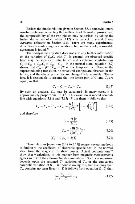
78 Chapter 3

Besides the simple relation given in Section 3.8, a somewhat more involved relation connecting the coefficients of thermal expansion and the compressibility of the two phases may be derived by taking the higher derivatives of equation (3.12) with respect to p and T (see Ehren/est relations in Section 8.1). There are many experimental difficulties in confirming these relations, but, on the whole, reasonable agreement is found. 23

Thermodynamics by itself does not give any further information on the variation of C"Cn with T. In general, the observed specific heat may be separated into lattice and electronic contributions Cn = C gn + Cen,Cs = C gs + C es . In the normal state, equation (3.9) shows that C gn = fJT 3, C en = yT at low temperatures. Now, in the superconducting transition, no structural changes are observed in the lattice, and the elastic properties are changed only minutely. There­fore, it is reasonable to assume that the lattice part of Cs and Cn are equal, so that

(3.17)

By such an analysis, Ces may be calculated; in many cases, It IS approximately proportional to T3. This variation is indeed compat­ible with equations (3.11) and (3.15). From them, it follows that

H 2V [ (T)2] Cn - Cs = Cen - Ces = 2n~; T 1 - 3 T"

and therefore

(3.18)

(3.19)

(3.20)

(3.21 )

These relations [equations (3.18 to 3.21)] suggest several methods of finding y, the coefficient of electronic specific heat in the normal state, from the magnetic threshold curves. Actual computations26

show that y calculated in this manner from magnetic measurements agrees well with the calorimetric determinations. Such a comparison depends upon the assumed T 3-variation of Ces or the equivalent parabolic variation of H c. Without invoking this, but assuming that Ces contains no term linear in T, it follows from equation (3.17) that

I. Cn - Cs 1m = y

1'-+0 T (3.22)

Electronic Specific Heat 79

The advantage of this procedure in not assuming the parabolic temperature dependence of He is to some extent countered by the need for making magnetic measurements down to very low tempera­tures. Where this has been done, the relation (3.22) is found to be obeyed very well.

While all these results show the internal consistency in the applica­tion of thermodynamic relations to superconductors, they do not throw much light on the microscopic mechanism of superconductivity. Very accurate measurements of Ces made since 1954 have revealed that at low temperatures it varies as

(3.23)

A typical result based on one of the early measurements is shown in Fig. 3.14. Departures from a T 3-law occur at very low temperatures, and thus probably escaped notice in the experiments made earlier. Similar small deviations of the Hc-T curve from the parabolic law were also observed. By analogy to the studies of Einstein's model of lattice vibrations (Section 2.4), the Schottky peak in paramagnetic salts (Section 4.9), and the roton specific heat in liquid helium II (Section 5.4), it may be inferred that such an exponential variation

0 ••

:: ,. ~ 0.1

v

O.O~

, -- C~,. y Tc 9.17 .'p (_ I.50 Ie T!

~ - -- Ce " Y Tc l I I leI'

"

~ "',

~ -~~ ~ ...

~ ........

~ 0.0 I

0.005

Fig. 3.14. Variation of C., in vanadium. 25

80 Chapter 3

of the specific heat is characteristic of the presence of an energy gap separating the normal and superconducting electrons.

In 1950, it was also found that the transition temperature 7;, depended on the isotopic mass M of the atom, 7;, '" IXM-I/2, which suggested that the interaction of the electrons with the lattice was somehow responsible for superconductivity. These ideas culminated in a satisfactory theory of simple superconductors by Bardeen, Cooper, and Schrieffer in 1957.

3.10. RECENT STUDIES

It is hardly possible here to do justice to the theoretical concepts underlying the Bardeen-Cooper-Schrieffer (BCS) theory, which has successfully correlated several effects discovered earlier and predicted new phenomena as well. The task is ameliorated by the existence of several texts.2 7 The theory shows that owing to the presence of virtual phonons, there is a tendency for the electrons to be correlated in pairs, called Cooper pairs. It requires an energy of approximately k7;, to break up this correlation, and the presence of such pairs allows a dissipationless flow of electric current. We shall content ourselves with a brief exposition of how the specific-heat studies fit into the theory.

The fact that an exponential variation of Ces [equation (3.23)] indicates the presence of an energy gap is easily visualized from Sec­tion 4.9, where it is proved that if two energy levels are separated by a gap e, the specific heat at low temperatures has a dominant term of the form exp( -e/kT). The detailed calculations of the BCS theory yield

C es - 1.44 7;, -T = 8.5 exp --­YeT

- 1.627;, = 26 exp --T---

~ 7;, or 2.5 < T < 6

for T

7 < ~ < 12

where the gap 2eo is related to 7;, by means of the relation

(3.24)

2eo = 3.52 k7;, (3.25)

The form of the specific-heat curves resemble equation (3.24) closely, and some values of 2eo/k7;, determined by fitting this equation are given in Table 3.1V. For widely different metals, the values do cluster around the idealized 3.52 of the BCS model, which incidentally assumes the metal to be isotropic.

Another simple prediction of the theory is that

C e.(7;,) = 2.43y7;, (3.26)

Electronic Specific Heat 81

Table 3.IV. Values of 2eo/kY:: Obtained from Ces-T Curves

Metal

In Ta 11 Sn v

3.9 3.6 3.2 3.6 3.6

analogous to equation (3.21). A few values shown in Table 3.V show that many metals do not deviate much from this equation. Con­sidering the simplicity of the model chosen for analysis and the wide variety of phenomena explained by it, the BCS theory must surely be considered as a significant advance toward the elucidation of a very complicated physical phenomenon.

Earlier, it was mentioned that the thermodynamic relations (3.12) to (3.16) are not very well satisfied for many alloys. Recent studies have shown that superconductors must be broadly divided into two categories. The superconductors of the first kind exhibit complete Meissner diamagnetism and seem to obey the thermodynamic rela­tions derived for them. The BCS model explains their behavior reasonably well. Superconductors of the second kind do not exhibit the full Meissner effect. As shown in Fig. 3.15b, the magnetic field begins to penetrate the specimen at a lower critical field Hcl , but the last traces of superconductivity are destroyed only at a much higher field H e2 . Thus, type II superconductors show even in longitudinal magnetic fields the characteristics similar to the intermediate state of an ordinary type I superconductor. Following some earlier sugges­tions by Ginzburg and Landau, Abrikosov showed that the mixed state between He! and He2 of a type II superconductor may be con­sidered as a bundle of normal filaments in a superconductive medium. The filaments, or fluxoids, which are the magnetic analogs of hydro­dynamic vortices, have special quantum properties and may also be pinned down by dislocations and other defects in the solid. Therefore,

Table 3.V. Values of Ces at Te

Metal

Hg Sn Al Ta Zn TI

Ce,(7;) 3.18 2.60

yI; 2.60 2.58 2.25 2.15

82

101

H­

I bl

Chapter 3

He,

Fig. 3.15. (a) Expulsion of flux in a superconductor of the first kind up to a critical field H,. (b) Incomplete Meissner effect in a superconductor of the second kind.

Flux penetration begins at H" and is complete at H,2'

the model allows the irreversibility of magnetization observed in type II superconductors. Further, the magnetization measurements do not have the same simple relationship to the measurement of electrical resistivity, as in type I superconductors. Many alloys are type II superconductors, and obviously the simple relations derived in Section 3.8 have to be generalized suitably.28 Indeed, careful measurements on ideal type II superconductors, clearly exhibiting the specific-heat singularities at the transitions, are only now avail­able. 29 The theory of Ginzburg and Landau, developed by Abrikosov and Gor'kov, explains many features of the behavior of type II superconductors, which are gaining technical importance in the generation of high magnetic fields. These matters are taken up at length in some recent reviews of the field. 27 ,30

REFERENCES

I. 1. L. Olsen, Electron Transport in Metals, Interscience, New York, 1962. 2. M. Born, Atomic Physics, Biackie, London, 1962, chapter 8. D. ter Haar, Elements

of Statistical Mechanics, Rinehart, New York, 1954, chapter 4. 3. C. Kittel, Solid State Physics, Wiley, New York, 1956, chapters II and 13. A.l.

Dekker, Solid State Physics, Prentice-Hall, New York, 1957, chapters 10 and 13. L. V. Azaroff and 1. 1. Brophy, Electronic Processes in Materials, McGraw-Hili, New York, 1963, chapters 7, 8, and 10.

4. 1. M. Ziman, Contemp. Phys. 3, 241,321,401 (1962); 4,1,81 (1963). 5. W. A. Harrison and M. B. Webb (editors), The Fermi Surface, Wiley, New York,

1960. 6. E. C. Stoner, Phil. Mag. 21, 145 (1936). 7. R. E. Gaumer and C. V. Heer, Phys. Rev. 118,955 (1960). 8. D. H. Parkinson, Rept. Progr. Phys. 21, 226 (1958). 9. 1. G. Daunt, Progr. Low Temp. Phys. 1, 202 (1955).

Electronic Specific Heat

10. P. H. Keesom and N. Pearlman, Handbuch der Physik, XIV(l), 282 (1956). 11. D. Pines, Solid State Phys. 1, 367 (1955). S. Raimes, Rept. Progr. Phys. 20,

(1957). 12. G. V. Chester, Advan. Phys. 10, 357 (1961).

83

13. P. L. Taylor, Phys. Rev. 131, 1995 (1963). S. K. Koenig, Phys. Rev. 135, A 1693 (1964).

14. N. F. Mott, Rept. Progr. Phys. 25, 218 (1962); Advan. Phys. 13, 325 (1964). 15. W. H. Lien and N. E. Phillips, Phys. Rev. 133, A1370 (1964). 16. W. Hume-Rothery, Electrons, Atoms, Metals, and Alloys, Iliffe, London, 1955,

chapter 29. 17. F. E. Hoare, in: Electronic Structure and Alloy Chemistry of Transition Elements,

P. A. Beck (ed.), Interscience, New York, 1963, p. 29. 18. G. J. van den Berg, Progr. Low Temp. Phys. 4, 194 (1964). 19. J. E. Zimmerman and F. E. Hoare, J. Phys. Chem. Solids 17, 52 (1960). J. E.

Zimmerman and H. Sato, J. Phys. Chem. Solids 21, 71 (1961). J. P. Franck, F. D. Manchester, and D. L. Martin, Proc. Roy. Soc. (London), Ser. A 263, 494 (1961).

20. A. W. Overhauser, J. Phys. Chem. Solids 13, 71 (1960). W. Marshall, Phys. Rev. 118, 1519 (1960). K. P. Gupta, C. H. Cheng, and P. A. Beck, J. Phys. Chem. Solids 25, 73 (1963).

21. V. A. Johnson and K. Lark-Horovitz, Progr. Low Temp. Phys. 2, 187 (1957). 22. P. H. Keesom and G. Seidel, Phys. Rev. 113, 33 (1959). 23. D. Shoenberg, Superconductivity, Cambridge University Press, Cambridge, 1952.

E. A. Lynton, Superconductivity, Methuen, London, 1962. 24. D. C. Rorer, H. Meyer, and R. C. Richardson, Z. Naturforsch. 18a, 130 (1963). 25. W. S. Corak, B. B. Goodman, C. B. Satterthwaite, and A. Wexler, Phys. Rev.

102, 656 (1956). 26. J. Eisenstein, Rev. Mod. Phys. 26, 277 (1954). B. Serin, Progr. Low Temp. Phys.

1, 138 (1955). 27. J. Bardeen and J. R. Schrieffer, Progr. Low Temp. Phys. 3, 170 (1961). J. M. Blatt,

Theory of Superconductivity, Academic, New York, 1964. G. Rikayzen, Theory of Superconductivity, Interscience, New York, 1965. J. R. Schrieffer, Theory of Superconductivity, Benjamin, New York, 1965.

28. R. R. Hake (in press). 29. T. McConville and B. Serin, Phys. Rev. Letters 13, 365 (1964). B. B. Goodman,

Phys. Letters 12, 6 (1964). 30. Proceedings of the IBM Conference on Superconductivity, IBM J. Res. Dev. 6,

1-125 (1962). Proceedings of the Colgate Conference on Superconductivity, Rev. Mod. Phys. 36, 1-331 (1964).

Chapter 4

Magnetic Contribution to Specific Heats

4.1. THERMODYNAMICS OF MAGNETIC MATERIALS

The behavior of magnetic materials at low temperatures is of widespread interest, be it in demagnetization techniques to produce very low temperatures or in the use of superconducting magnets. Therefore, it is worthwhile to consider the specific heats of magnetic materials separately. It is well known that the magnetic energy depends upon the operative magnetic field H, and so it is first necessary to inquire how the specific heat is defined for a system capable of magnetization.

For a simple fluid, the basic thermodynamic relation used in Chapter 1 was

T dS = dE + dW = dE + P dV (4.1)

If the fluid is magnetizable, a term M·dH must be added to dW as the work done in changing the magnetic field. For simplicity, the scalar product M ·dH may be replaced by M dH where M, the mag­netic moment of the substance, is interpreted as the component of M in the direction of H. Then

T dS = dE + P dV + M dH = dE' + P dV - H dM

where E' = E + M H. It is somewhat arbitrary whether E or E' is considered as the internal energy of the substance. This depends on whether the energy M H arising from the simultaneous presence of the field and the body is included in the energy content of the field or of the body. In several cases, it is advantageous and logical 1 to use E' as the internal energy. Further, in the problems of interest here, the mechanical work P dV may be neglected in comparison with the magnetic part - H dM. So the fundamental relation may be written as

T dS = dE' - H dM 84

(4.2)

Magnetic Contribution to Specific Heats 8S

A comparison of equations (4.1) and (4.2) shows immediately that all the relations derived in Chapter 1 may be taken over to the magnetic case simply by replacing P and V by Hand - M, respectively. The principal magnetic heat capacities, CH at constant field and CM at constant magnetization, are

CM = (dQ) = T(as) (4.3) dT M aT M

The equations (1.12) and (1.14) between Cp and Cv are transformed into

T(aMjaT)~

(aMjaHh (4.4)

while the relation (1.16) giving the ratio of isothermal to adiabatic compressibility becomes

(aMjaHh CH

(i3MjaHh CM (4.5)

In general, (aMjaH) depends upon the shape of the body. For a long rod set parallel to H, the field Hi inside the body is the same as the outside field H, whereas for other orientations and shapes, appropriate coefficients of demagnetization have to be introduced. Assuming this to be done, the differential molar susceptibility X may be intro­duced by the relation

aM aH = X (4.6)

where M refers to the moment per mole. The correspondence C p +-+ CHand C" +-+ C M suggests that C M

is the quantity of greater theoretical interest. This is true to some extent because in an "ideal" paramagnetic materiaL which obeys the relation M = f(HjT), CM is independent of the external field. A simple way of showing this is to write the magnetic analogs of equation (1.17), namely,

(4.7)

For an "ideal" paramagnet, M = f(HjT) or H = Tf-l(M). There­fore, (iJCMjiJMh = 0, whereas CH depends upon H.

These relations concerning the magnetic contributions to the heat capacity and hence to the entropy of a substance are of importance in the process of adiabatic demagnetization. A full discussion of the question may be found in the many reviews on the subject. 2

86 Chapter 4

4.2. TYPES OF MAGNETIC BEHAVIOR 3

The molecules of most materials have no permanent magnetic moments. Under such conditions, an applied field H induces a magnetic moment in the electronic system of the molecules which is in a direction opposite to that of H; this behavior is said to be dia­magnetic. Diamagnetism is independent of temperature, and so it is of little interest in specific-heat studies. Some molecules, oxygen, for example, have elementary magnetic moments f1; at high temperatures, they are ordinarily oriented at random. On applying a magnetic field, there is a preferential orientation of the moments along H, resulting in a magnetization parallel to H (paramagnetic behavior). At low temperatures, an ordered arrangement of the elementary magnets is possible. This ordering process was attributed pheno­menologically to internal magnetic fields by Weiss in 1907, but in 1928 Heisenberg showed that it is due to the quantum-mechanical exchange interaction between neighboring electrons. An ordered state with parallel spins and therefore parallel magnetic moments (Fig. 4.1b) produces a large spontaneous magnetization even in the absence of H. In this ferromagnetic state, M becomes a nonlinear function of H and hysteresis effects are also present.

The exchange interaction is able to overcome the thermal randomization of the spins at a sufficiently low temperature. The Curie temperature 7;" below which the spins become ordered, is as high as 1080 0 K for iron and less than 10 K for some alums. However, the ordered state need not always be ferromagnetic, as was shown by Neel. In some cases, the adjacent spins may be aligned anti parallel (Fig.4.1c). In this antiferromagnetic state there is no net spontaneous magnetization, but hysteresis is present and the susceptibility shows a sharp maximum at the transition temperature (Neel point). In a few cases, alternate magnetic moments are unequal and become arranged with adjacent spins antiparallel (Fig. 4.1d). This ferri­magnetic state is macroscopically similar to a ferromagnetic state, but the substances-ferrites and garnets find important practical

11111111 11111111 11111111 11111111 (a) (b) (e) (d)

Fig. 4.1. Schematic order-disorder state in a lattice of elementary magnets: (a) para­magnetism-disordered spins; (b) ferromagnetism-parallel spins; (c) antiferro­magnetism-adjacent spins antiparallel; (d) ferrimagnetism-adjacent unequal spins

antiparallel.

Magnetic COOtribUtiOD to Specific Heats 87

applications-are poor conductors of electricity. Other types of ordering in which the spins are arranged along spirals are also possible (Section 7.6), and simple surveys of para-,4 ferro-, 5 antiferro-,6 and ferrimagnetic 7 states are available.

It is clear that, if the atoms or molecules of a substance possess permanent magnetic moments, the magnetic state depends very much upon the temperature, which means that interesting effects may be expected in the specific heats. In discussing them, it is convenient to start from the ordered state at low temperatures and then to pass on to the behavior as the temperature is raised.

4.3. SPIN WA VES-MAGNONS

The ideal ordered state described above exists only in the absence of thermal agitation. Taking first the case of ferromagnets, the spins at the lattice sites are aligned at OaK along, say, Z so that the angular momentum hs is along Z. At a finite temperature, the spins at some sites j may be excited to higher energy states, i.e., point in other directions. Such distributions may be Fourier-analyzed into a set of waves. A spin wave may then be described as a sinusoidal disturbance of the spin system. The usefulness of describing a ferromagnet at finite temperatures as a superposition of spin waves was pointed out by Bloch in 1930. It permits a correlation of the various magnetic and other properties. A full description of the subjectS is outside the scope of the present work, and only a qualitative derivation9 of the spin wave spectrum in a ferromagnet can be given here. Unfortun­ately, this conceals some of the difficulties involved in the concept of spin waves, which are treated at length elsewhere.s

For simplicity, consider a linear ferromagnetic chain with a small field H 0 along - Z. Then the spins will all be pointing up with angular momenta hSi about Z. Further, Si = JlJgfJ = JlJhy where fJ = he/4nmc is the Bohr magneton, y = ge/2mc is the magneto­mechanical ratio, and g is the Lande factor equal to approximately 2 in ferromagnets. Classically, at OaK all the spins will precess in phase about Z at the Larmor frequency (00 = yH o. If now a spin wave is excited, the situation will be as shown in Fig. 4.2a. The spins are no longer in phase, and the phase angle between successive spins is equal to qa, where a is the lattice constant and 2n/q is the wave­length.

In an effective field H eff' each spin, because of its magnetic moment, will experience a torque ELi X Heff = yhs i X H eff . This torque is equal to the time rate of change of angular momentum

d(hsi) ~ = yhsi X Heff

88 Chapter 4

Qq., 9· / / I 000

.....

(0)

o (b) leJ

Fig. 4.2. Classical picture of a spin wave q in a linear ferromagnetic chain.

The effective field is calculated from the Hamiltonian [compare equation (4.18)]

Yfi = -gf3Si· (Ho + ~~~Sj) = -gf3si·Herr

where the sum :r.j is over the two near neighbors and J is the quantum­mechanical exchange constant. Using this value of Herr,

d(hs i) (2J) -- = yhs· x H 0 + - L s· dt ' gf3 j J

(4.8)

If R is the amplitude of precession, Si x Ho = sHo sines, Ho) = RHo. Figures 4.2 (a and b) shows that the resultant of OP 1 and OP3 is 20Q where P2Q = tRq2a2, and from Fig. 4.2c cjJ = LP20Q = tRq2a2s- 1•

Therefore, the right-hand side of equation (4.8) is equal to yh[RH 0 + (2J jgf3)sRq2a2]. The left-hand side is hw'R, where w' is the angular velocity of precession, and so

w' = yHo + 2J sq2a2 gf3

The Larmor frequency of the spin system is yH 0, and the frequency of the spin wave itself is

(4.9)

In a three-dimensional crystal, the same dispersion law wex:. q2, first found by Bloch, is obeyed, and the general ferromagnetic spin

Magnetic Contribution to Specific Heats

wave frequency may be taken as 2Jsa2 2

Wq = rtf - h- q

89

(4.10)

The constant rtf depends upon the details of the crystal structure and has been calculated in several practical cases. B The same W ex q2

is also obeyed by the spin waves in a ferrimagnet. However, in anti­ferromagnets, special considerations come into play in defining the normal modes of disturbances. It was first shown by Hulthen that the spin-wave spectrum is given as

2J'sa2

Wq = rta - h- q (4.11)

where J' is the magnitude of the exchange constant. The antiferro­magnetic spectrum is linear in q, unlike the quadratic dependence in ferro- and ferrimagnets. To establish equation (4.11) would require a longer discussion than is warranted here, and so it suffices to mention the references to elementary9 and rigorousB derivations.

It is interesting to compare the spin waves with the lattice waves analyzed in Chapter 2. At low frequencies, the normal modes of a lattice have a dispersion relation W ex q, whereas the allowed modes in the spin system may be either W ex q2 as in ferromagnets or W ex q

as in antiferromagnets. A set of mass points connected by elastic springs will form a model for lattice vibrations. A model for spin waves will be a set of arrows, each connected to its two neighbors by torsional springs. The angular displacement of a spin out of the line with its neighbors gives rise to a torque proportional to the excess displacement and tending to restore equilibrium. The analogy with lattice waves is actually very deep. The spin waves may be quantized into magnons, which play the same role in magnetic phenomena as phonons do in lattice dynamics. Magnons and phonons obey Bose­Einstein statistics. These similarities have been very fruitful in the study of magnetic systems.

4.4. SPIN WAVE SPECIFIC HEATS

The fact that magnons obey Bose statistics allows easy calculation of the low-temperature thermal properties of magnetic materials. It was seen in Chapter 2 that at a temperature T the mean energy of a Bose oscillator of angular frequency W is hw/[exp(hw/kT) - 1] [equation (2.8a)] and that the number of energy states between momenta p and p + dp is (4nV/h3)p2 dp [equation (2.18)]. Using the dispersion relations (4.1 0) and (4.11), the specific-heat contributions at low temperatures can be easily derived.

90 Cbapter4

(4.12)

The upper limit of integration over q cannot be specified without detailed analysis, but at low temperatures the upper limit for x may be taken as infinity without serious error and the integral may be evaluated suitably. The specific heat now follows as

dE (kT)312 CM = dT = cfNk 2Js (4.13)

where the constant C f has been calculated for several crystal struc­tures.8 For example, C f '" 0.113 in a simple cubic arrangement of spins. Equation (4.13) is an important result, that at low temperatures the ferromagnetic contribution to specific heats is proportional to T312. A similar T312-variation is obeyed by the saturation magnetiza­tion of ferromagnets, for which the T312 behavior had been observed for a long time. In specific heats, the measurement of spin wave contri­butions has been only recently successful.

In metals (Chapter 3), the conduction electrons give a specific heat proportional to T, the phonons give a T 3 -term, and, if the above magnetic term is added, the low-temperature specific heat will be of the form

Cv = yT + f3T 3 + bT312

The temperature variation of the heat capacity will be dominated by the term with the lowest power of T, namely, the electronic term. With a few exceptions discovered recently, most ferromagnets are metallic; therefore, a clear resolution of the magnetic T 312-term is a matter of considerable experimental difficulty. Not surprisingly, the spin wave effects were not easily observed in the specific heats of ferromagnets, although the magnetic measurements had borne out the theoretical predictions. The situation is quite different in ferrimagnets. They are electrical insulators, and in the absence of free electrons the specific heat is of the form

Cv = f3T3 + bT312

At low temperatures, the spin wave is dominant, and a plot of CT- 312 against T312 should be a straight line. The first such experiments

Magnetic Contributioo to Specific Heats

~

" If' ~ If' ."

~ U

) ~

~ J

200

100

~ (deg K~)

Fig. 4.3. Low-temperature specific heat of YIG showing the spin wave T3/2_

contribution. 10

91

were made on magnetite Fe304 by Kouvel in 1956; since then, similar measurements have been made on several garnets, ferrites, and very recently on some ferromagnetic insulators. Figure 4.3 shows a typical result for yttrium iron garnet (YIG), with clear evidence for the T 3 /2 _term. 10 The exchange constant J may also be obtained from various other experiments, such as magnetic resonance and neutron scattering. The agreement among the values of J is fair, when the large corrections for demagnetizing effects and anisotropy are taken into account.

Going now to the case of antiferromagnets, the dispersion relation OJ = lY.a(2J'sa 2/h)q means that

E = 4nV f 21Y.J'sa2q3 dq

o exp(2IY.Jsa2q/kT) - 1

92 Chapter 4

C(J/ mole'd"lll

30

w ~------------------------~---7~-------------------1

10

29.5 so 100

T(deg K)

Fig. 4.4. Heat capacity of MnC03 (circles and thick lines) and CaC03 (thin lines) showing antiferromagnetic contribution. I I

At low temperatures, the upper limit for x may again be taken as infinity, and the specific heat becomes

eM = CaNk(~;sY (4.14)

The constant Ca has been calculated for several types of lattices. The T3 spin wave specific heat in antiferromagnets is strikingly different from the T3/2-dependence in ferromagnets. The temperature depen­dence is of the same form as the lattice contribution in the Debye T3-region. This makes an experimental separation of the spin wave and lattice specific heats almost impossible in metals and very difficult in nonmetallic antiferromagnets. In the carbonates of manganese and cobalt, the antiferromagnetic T 3-contribution is about ten to twenty times larger than the lattice term, as may be seen in Fig. 4.4, where the specific heat of MnC03 is compared with that of CaC03, which has no magnetic contribution.!! The experimental values agree very well with those calculated from magnetic measurements.

It must be added that the spin wave specific-heat relations (4.13) and (4.14) hold good at moderate temperatures only. At very low

Magnetic Contribution to Specific Heats 93

temperatures, some of the approximations made above are not valid and the specific heat may decrease exponentially. At high tempera­tures, interactions among magnons give rise to other terms, as shown in detail by Dyson, and the simple spin wave picture is no longer very useful. For the sake of simplicity, these details8 are left out here.

4.5. THE WEISS MODEL FOR MAGNETIC ORDERING

As mentioned earlier, the ordered ferro-, ferri-, or antiferro­magnetic states go over into the paramagnetic state at sufficiently high temperatures. The change in the magnetic properties is accom­panied by a sharp peak in the specific-heat curve at 7;,. Figure 4.5 shows the typical example of nickel. The magnetic contribution eM is obtained by subtracting the lattice and electronic terms from the total Cv ' The behavior near 7;, is typical of a general class of coopera­tive transitions, which will be discussed at length in Chapter 7.

Historically, it was Weiss who in 1907 gave a simple explanation of ferromagnetism. A few years earlier, Langevin had shown that the

10

8

I- 1 . /

./ \..

,.-

~ y

/

f r--I-" C,

6

II If

"1 c. A

:..--:...--- k2:: .\cM Cp - Cy

---:- J l\. o o 200 600 800

T (dog K)

Fig. 4.5. Heat capacity of nickel (in calfg-atom'deg) showing the magnetic contribution eM besides lattice and electronic terms.

94 Chapter 4

competition between the magnetic field H tending to align the elemen­tary magnets fJ. and the thermal agitation causing a random arrange­ment results in a net magnetization of the form

M = N /1 tanh (~~) (4.15)

Langevin's theory explained many aspects of paramagnetic behavior­in particular, Curie's law, that the susceptibility varies as 1fT, arises because for ordinary fields and temperatures flH/kT ~ 1. Weiss suggested that because of the magnetization of the other parts of a solid there is an internal magnetic field aM (a a constant) and that the effective field acting on the elementary dipoles is

Herr = H ext + aM

Substitution of H eff in place of H in equation (4.15) shows that even in the absence of an external field H ext there is a spontaneous magnetiza­tion given by the implicit equation

Ms = N/1 tanh --(Ms~) N/1 T

(4.16)

where ~ = aN /1 2 /k. This is the ferromagnetic state. Weiss's theory also explained hysteresis and other features of M-H ext curves. For many metals, equation (4.16) satisfactorily describes the variation of M s with T, except very near the transition temperature ~. The moment /1 comes out to be equal to the Bohr magnet on he/4nmc, showing that ferromagnetism is due to the magnetic moment of electrons. [As a matter of fact, equation (4.15) is the quantum­mechanical expression for particles of spin th.]

The energy of magnetization in the absence of H ext is

and so the magnetic contribution to specific heat is

1 dM 2

C M = -2"a dT (4.17)

The magnetic specific heat given by the Weiss model is shown in Fig. 4.6. eM steadily increases from zero at T = 0 to a maximum ~R at T = ~. This maximum is followed by a discontinuous drop to eM = 0 in the paramagnetic state T > ~. No latent heat is liberated at ~, and the transition in the Weiss model is a phase change of the second order (see Section 8.1).

Magnetic Contribution to Specific Heats

I

2R , ,

I

/ 1 /

~ / \

/ \

/ ",'/ \ , /' ....

/ - -o o 0.2 0 .4 0.6 0.8 1.0 1.2 1.4

Fig. 4.6. Schematic variation of magnetic heat capacity near 7; in the Weiss model (full line) and in statistical theories (broken lines).

95

The experimental values of CM, as seen in Figs. 4.4 and 4.5, follow the general trend in being small at low temperatures and beginning to rise as 7;, is approached. Near 7;" there is not even qualita­tive agreement with the above theory. C M often rises to a value much higher than the predicted maximum; furthermore, the specific-heat curve has a "tail" above the transition. CM decreases sharply, no doubt, but instead of falling abruptly to zero it lingers on for a con­siderable range of temperatures before becoming immeasurably small.

The phenomenological theory may be suitably modified to give a small "tail" to the specific-heat curve,12 but the agreement is not very much improved. It is generally believed that an explanation of the behavior of ferro- and antiferromagnets near 7;, belongs to the realm of proper statistical theories.

4.6. THE HEISENBERG AND ISING MODELS

Very soon after the development of quantum mechanics, Heisen­berg (in 1928) gave an explanation of the origin of Weiss's internal magnetic fields, whose large magnitudes of around 105 Oe remained puzzling. On account of the Pauli exclusion principle, two electrons with spins SI, S2 have an interaction energy of the form - 2Js I . S2,

where the exchange integral J is a function of distance. For large separations of the electrons, J is very small, but for spacings of the

96 Chapter 4

order of a few Angstroms the exchange energy becomes large enough to be comparable to chemical binding energies. Thus, if the energy were written in terms of the electronic magnetic moments /L, it would be of the same form and magnitude as the internal magnetic energy in the Weiss model, even though it is basically electrostatic in origin. If 1 were positive, a parallel (ferromagnetic) alignment of spins would be favored, while a negative 1 results in anti parallel alignment.

The statistical theory of magnetic systems thus involves the calculation of the partition function L exp( - Er/kT) of the system. With the general form of the exchange interaction, the calculations are so prohibitively complicated that it is normal to make two stages of approximations. The Heisenberg model assumes that, since 1 falls off rapidly with increasing distance, it is enough to take the interactions as extending only to the nearest neighbors. Thus the energy of the system in this model is

E(Heisenberg) = -21 I Si' Sj - flU' I Si (4.18) i.j

where L is over all pairs of direct neighbors. This model has been quite successful in explaining, for example, the spin waves at low temperatures (Section 4.3). However, even this approximation in­volves formidable difficulties, so that in many statistical problems a further simplification is commonly used, though the model was intro­duced slightly earlier by Ising. In the Ising model, the scalar product Si . Sj is replaced by SizSjz on the basis that if Z is the direction of alignment, the expectation value of S in X, Y directions is zero. Then

E(Ising) = - 21 L SizS jz - flH L Siz (4.19) i,j i

where L is again over pairs of adjacent neighbors. The Ising model is a scalar problem in that it deprives magnetism

of its intimate connection with the angular momentum of electrons. Further, it does not admit a spin wave picture at low temperatures. Hence, it may be considered a poor model for magnetic studies. However, near or above 7;" the statistical enumeration of the states, which is correctly taken into account, assumes dominant importance in the thermodynamic and other properties of the system. Therefore, a large amount of theoretical work has been done on the behavior of the simple Ising model near 7;" where its deficiencies are unimportant. There are two reasons for the great interest in the field: In the first place, the Ising and Heisenberg models furnish instructive theoretical schemes not only for magnetic transitions but also for other coopera­tive transformations, which will be discussed in Chapter 7. The Ising model is the simplest one which appears to reproduce many of the

Magnetic Contribution to Specific Heats 97

features observed experimentally. Secondly, the general problem for a three-dimensional solid has remained so far an unsolved challenge. The exact solution for a two-dimensional Ising model was given by On sager in 1944, but even this is a remarkable tour de force to be savored only by professional theoreticians. 13

It is now superfluous to add that the solutions of the Heisenberg and Ising models, even in their approximate form, are far too sophis­ticated to be reproduced here. As regards the specific heat, which is the prime concern in this text, the two-dimensional Ising lattice exhibits a logarithmic singularity:

eM ~ A log (T - TJ .. . ~ B log (~ - T) .. .

(4.20)

where the constants A, B have been calculated for several lattices. In a three-dimensional case, such exact relations are not yet available, and various approximate calculations have been made. The nature of the singularity, whether an inverse power of IT - 7;,1 or logarithmic in IT - ~I, cannot be described with certainty, although for a diamond­type Ising lattice the approximations have been carried sufficiently far to suggest a logarithmic infinity in specific heat below the ferro­magnetic transition. 14 To be fair, it must be mentioned that a logarithmic singularity at the cooperative transition had been re­vealed by calorimetric measurements performed somewhat earlier (Figs. 4.9 and 5.5). Above 7;, the experiments can be fitted to a loga­rithmic term in some cases and to a power law singularity in others.14a

It is also possible to estimate the ferromagnetic transition tem­perature 7;" as well as the magnetic part of the entropy S and internal energy E that are removed at the transition. For a fcc lattice, the values are

2k7;,/zJ 0.68 0.82

(S~ - SJ/k 0.27 0.10 (4.21)

0.44 0.15

Here z is the number of nearest neighbors and J is the exchange constant. The values are for spin !, and the first column refers to the Heisenberg model and the second to the Ising model. The entropy values show that the Heisenberg model has a larger tail on the high­temperature side than the Ising model. For bcc or other types of lattices, the constants in (4.21) are slightly different. Similar small variations arise for spins greater than !. In particular, the specific

98 Chapter 4

heat on the high-temperature side rises more rapidly for larger spins. Antiferromagnetic transitions may be studied similarly, but calcula­tions are scanty. A schematIc variation of tilt: s{JC\.:iu\" ~-,.oaL "cur I;, is shown in Fig. 4.6.

In contrast to these approximate values, which depend upon the model chosen for calculations, a very general result may be given for the total magnetic entropy SM. It is well known that a particle with spin sh has 2s + 1 quantized orientations. In a field H, the levels have slightly different energies, but in the absence of H the energies are all equal and there is a 2s + 1 degeneracy in the state of the system. The entropy corresponding to this is kIn (2s + 1) per particle, which is the entropy that comes into play here. The rule

SM = R In (2s + 1) per mole (4.22)

has been verified in many cases. 15 Only a small part of this entropy is removed as the substance is cooled to T" from a high temperature. This percentage is slightly larger in a Heisenberg model with its larger tail above T". Most of the ordering takes place below the transition.

4.7. SPECIFIC HEATS NEAR THE TRANSITION TEMPERATURE

It is only recently that careful experimental studies have been made to check the various predictions of the statistical theories; on the whole, reasonable agreement is found. 16 As an example of ferromagnets, the complete magnetic and calorimetric studies 1 ? on copper ammonium and copper potassium chlorides, Cu(NH4 hCI4 ·

2H 2 0(T" = O.70 0 K) and CuK 2CI4 ·2H2 0(T" = 0.88°K), may be con­sidered. Below about O.5T", the specific heat follows the variation given by this spin wave theory (Section 4.3). For the ammonium salt, the exchange constant Jlk given by the spin wave variation is about 0.28 oK, compared to the values of approximately 0.30oK calculated from the Curie-Weiss constant and approximately 0.29°K derived from the behavior of the specific heat in the paramagnetic state T> T". Near T", the statistical theory suggests that the specific heat is a function of TIT" only; Fig. 4.7 shows how closely this is verified. (The lattice contribution is negligible at these low temperatures.) The entropy calculated from the full line has a value of 5.81Imole·degK, whereas the theoretical value for s = t of Cu 2 + ion is R In 2 = 5.761Imole·degK. Further, the authors obtain 2kT"lzJ = 0.75, (Soo - SJlk = 0.22, (Eoo - Ec)/kT" = 0.38. These values are in between the numbers given in (4.21), although the Heisenberg model gives a good explanation of the other properties of the substance. A part of the discrepancy may be due to the bcc structure of these salts,

Magnetic Contribution to Specific Heats 99

15~----------,-------------------------.-----------~

o "

10

5

o~----------~----------~----------~~----------~ 1.0 1.5 2.0 T/ Te 0.5

Fig. 4.7. Heat capacity of CuK2CL,'2H20 (7;, = O.882°K, circles) and Cu(NH4hCI4 '2H20 (7;, = O.704°K, triangles) plotted as a function of T/7;,.16

whereas equation (4.21) refers to a fcc lattice. Support for this view is given by the fact that a Heisenberg model for a bcc lattice gives 2kTclzJ = 0.72, in much better agreement with the experiments.

Antiferromagnetic transitions are exemplified by the study18 of nickel and cobalt chlorides, NiCI2·6H20(TN = 5.34°K), CoCI2·6H20 (TN = 2.29°K). The specific heat of the nickel salt is shown in Fig. 4.8, while that of the cobalt salt is similar except for the change in the Neel temperature. The lattice term, which is nearly the same in both saits, was found from the T 3-behavior of the lattice specific heat and the T- 2-variation of the paramagnetic specific heat at T~ TN (com­pare Section 4.9). The magnetic specific heat is obtained by subtract­ing the lattice contribution from the total specific heat. Because of the influence of the crystalline electric field upon the electronic levels of the transition metal ions, one should expect s = ! for the cobaltous ion and s = 1 for the nickelous ion. The magnetic entropy was equal to 9.131/mole·degK for the nickel sait, which is within 1 % of R In 3. That of cobaltous chloride was 5.80 l/mole·degK ~ R In 2. The exchange constant IJI/k has a value of approximately 1.6°K for COC!2·6H20 if calculated from the total ordering energy and about 1.5°K if calculated from the Neel temperature. Of more interest is

100

1 ." .. 1 8 Q. v

Chapter 4

J

O~~~---L __ ~ ____ L-__ ~ __ -L __ ~ ____ L-__ J-__ -L __ ~

o 10 14 16 18 20 22

T(deg K)

Fig. 4.8. Heat capacity of NiCl2 ·6H20 .18

the behavior of eM found near TN (Fig. 4.9). The data appear to suggest that the specific heat becomes logarithmically infinite at the Neel temperature. This singularity and the similar behavior found in liquid 4He (Fig. 5.6) are of special interest because Onsager's solu­tion for a two-dimensional cooperative transition shows a logarithmic infinity, while no firm predictions are as yet available for a three­dimensional case.

4.8. PARAMAGNETIC RELAXATION

Specific-heat studies in paramagnetic salts are important in two respects. In the first place, the attainment of temperatures much lower than 10 K by adiabatic demagnetization techniques involves a thorough knowledge of the magnetic entropy which can be extracted from the system. Secondly, paramagnetic saIts furnish an interesting class of specific-heat anomalies, namely, the Schottky peak. Before these matters are taken up in detail, it is convenient to discuss a special method of measuring specific heats which is very useful when they are not easily separated from the lattice contributions.

The method is based on paramagnetic relaxation,3.4 discovered by Gorter. If a magnetic field is applied to a paramagnetic salt, the internal energy of the system is changed. It is found that the time

Magnetic Contribution to Specific Heats 101

taken for the transfer of the heat of magnetization from the dipoles to the crystal lattice (spin-lattice relaxation time) is much longer than the time needed for the establishment of thermal equilibrium among the dipoles themselves (spin-spin relaxation time). On suddenly changing H, the dipoles very quickly (in about 10- 10 sec) follow the field, but the magnetic energy is given to the lattice only in a leisurely (of the order of 10 - 6 sec) fashion. Therefore, for any variation of H over a time long compared to the spin-spin relaxation time but short compared to the spin-lattice relaxation time, the dipoles are in equilibrium among themselves but do not exchange heat with the lattice. A measurement of the variation of M under such conditions gives the adiabatic susceptibility Xs. The normal DC measurement yields the isothermal susceptibility XI" Equations (4.4) to (4.6) now show that

or (4.23)

As pointed out first by Casimir, du Pre, and de Haas in 1938-1939, the lattice temperature is not changed during the measurement, and so the lattice specific heat does not enter the calculation.

102 Chapter 4

By this technique it is possible to measure magnetic contributions to specific heats at liquid-nitrogen temperatures, where they may amount to only 10- 6 of the total heat capacity of the salt. Since the spin-lattice relaxation time is about 10- 6 sec at these temperatures, the adiabatic susceptibility must be determined at radio frequencies. At liquid-helium temperatures the spin-lattice relaxation time is usually of the order of 10- 3 sec and audiofrequency measurements suffice. The details of the experimental techniques are thoroughly discussed by Benzie and Cooke. 19 At very low temperatures ( ~ 10 K), the heating produced in AC measurements is considerable, and direct calorimetry is preferred. At these temperatures, the lattice specific heat is so small that the entire specific heat measured calorimetrically may be taken as arising from magnetic effects. At higher temperatures, the paramagnetic relaxation technique is very useful, because the lattice and magnetic terms are nearly comparable and not easily separated out.

At very low temperatures, since the spin system can exist for an appreciable time without interacting with the lattice, it is advantageous in magnetic studies to attribute a separate (spin) temperature and specific heat to the spin system. Discussions of such nonequilibrium concepts can be found in the treatises on magnetic resonance and are not appropriate here.

4.9. SCHOTTKY EFFECT

It is well known that a particle with spin sh has 2s + 1 possible orientations of the spin; in a magnetic field, the particle has a number of discrete energy levels. This spacing of the quantized energy levels is reflected in the specific heat in an interesting way. Consider for a moment a system with two levels, L1 apart. At T ~ L1/k, the upper level will scarcely be populated, whereas at T ~ L1/k both levels will be nearly equally populated. Only at temperatures comparable to L1jk will transitions from one level to another take place in appreciable amounts. This rapid change in the internal energy corresponds to a large specific heat which becomes zero at both high and low tempera­tures. Thus there is the intriguing possibility of a hump in Cv, which will in general be superimposed on the lattice and other contributions.

A general problem of this kind was considered by Schottky in 1922. Suppose there is a system in which the particles can exist in a group of m levels, separated from the ground state by energies C1' cz, ... , Cm and with degeneracies g1' g2' ... , gm' Using the Boltzmann factor exp( - c/kT), the probability of a particle occupying the rth

Magnetic Contribution to Specific Heats

level is gr exp( - erik T)

L gr exp( - er/kT) n

103

With N independent particles in the system, the mean energy at a temperature Tis

m

N L ergr exp( - er/kT) E = r=O

m

L gr exp( - er/kT) r=O

(4.24)

The specific heat is obtained by calculating dE/dT. The simple case of two levels illustrates all the features of such calculations. For a two-level system, equation (4.24) becomes

E = Ng1el exp( -edkT) go + gl exp( -edkT)

and the Schottky specific heat is

Nd go exp(edkT) C Sch = - - c:-c--.,---:-=--=':'-,.-::-=:::-=

kT2 gl [1 + (gO/gl) exp(edkT)]Z

( b)2 go exp(b/T) = R T gl [1 + (gO/gl) exp(b/T)jZ

(4.25)

where b = edk is the energy separation measured in degK. CSch is plotted in Fig. 4.10 for a few values of g dgo.

The qualitative remarks made earlier about the behavior at low and high temperatures may now be made quantitative. From equa­tion (4.25) it is easy to see that

(4.26)

(4.27)

The specific heat attains a maximum value at an intermediate tempera­ture Tm given by

( go) exp(~) = (b/Tm) + 2 g 1 Tm (b/Tm) - 2

(4.28)

and the maximum itself is equal to

CSch(max) = ~ ~m[(:J2 -4J (4.29)

104 Chapter 4

, .0

0.8

0.6

J 0.4

0.2

0.1 0.4 0.6 0.8 \.0 1.2 1.4 1.6 \.B 2.0

T /;

Fig. 4.10. Schottky heat capacity of a two-level system for several values of f,,/f,o'

Thus if go/g 1 = I, the maximum occurs at Tm = 0.42<5 and has a value CSch(max) = 3.61/mole·deg. Table 4.I gives Tm/<5 and CSch(max) for several values of g J!go. When these values are compared with the typical lattice and electronic contributions of 10- 2 l/mole·deg at 4 OK, it is evident that a Schottky peak occurring at liquid-helium tempera­tures will dominate the variation of specific heat (see Fig. 4.11).

If CSch is isolated from the observed total specific heat, by the methods to be discussed below, there are several ways of finding <5 and g J!go. The position and magnitude of the peak, the behavior at high temperatures (CSch'T 2 = constant) or at low temperatures (log (CSch'T 2 ) linear in I/T) may all be used. This, of course, assumes that there are only two energy levels to be considered. If more levels are involved, the full equation (4.24) has to be used, or, alternatively,

d2(RTlnz) -2 d2 lnz CSch = T dT2 = RT d(1/T)2

TABLE 4.1

C Sch (max) g,/go l/mole'deg Tm/o Total entropy

0.5 2.00 0.448 R Ini 1.0 3.64 0.417 R In 2 1.5 5.06 0.394 R In! 2.0 6.31 0.377 R In 3 5.0 12.0 0.320 R In6

Magnetic Contribution to Specific Heats 105

where

z = Lg.exp(-:~) Apart from the behavior CSch oc T - 2 at high temperatures, no simple results can be given. In such cases it is necessary to start with some schemes of energy levels derived either theoretically or from suscepti­bility, paramagnetic resonance, and other data. The specific-heat curve then serves as a check on the correctness of the assumed model.

The entropy associated with the Schottky peak may be obtained by integrating CSch • T- 1 ; the values for the two-level case are given in Table 4.I. These results may also be obtained by enumerating the possible configurations of the system, as was done with equation (4.21). For example, if there are m levels of equal degeneracy, the extra entropy is R In m per mole. In the two-level case, S = R In [1 + (gdgoH Usually, a comparison of the theoretical and experimental values of the excess entropy serves to verify the correctness of separ­ating out CSch from the observed total specific heat.

The problem of getting CSch from the observed specific heat by subtracting the lattice and other contributions is one of consider­able difficulty. If the Schottky peak occurs at low temperatures, the lattice term may be taken as f3T 3 . At temperatures well above the peak, CSch oc T- 2, and the total specific heat will be of the form C = f3T 3 + BT- 2• Thus a plot of CT2 versus T 5 should be a straight line, which permits the desired resolution to be carried out. The magnetic contribution in Fig. 4.9 was obtained from Fig. 4.8 in this manner. For this separation to work, the lattice term must be propor­tional to T3 and the two terms must be of similar magnitude. If this restriction cannot be satisfied, it is usual to take for Clatlice the specific heat of a salt of similar composition and same crystal structure, but which does not have an anomaly. The case of MnC03 and CaC03

(Fig. 4.4) is an example of this type of analysis. In some cases, the magnetic contribution may be evaluated separately from measure­ments of paramagnetic relaxation or adiabatic demagnetization from different magnetic fields. In general, the Schottky term, if present at liquid-helium temperatures, is so large a fraction of the observed specific heat that small errors in evaluating the lattice corrections are not serious.

4.10. SPECIFIC HEAT OF PARAMAGNETIC SALTS

Paramagnetic salts, in which the magnetic dipoles have energy levels with spacings of approximately 1 to lOOK, form the natural examples of simple systems exhibiting a variety of Schottky peaks. That such a close relationship should exist may be inferred in the

106 Chapter 4

following way. For the magnetic moment of a paramagnet, Langevin's theory gives an expression of the form

M = NJLtanh(JLH/kT) (4.15)

In a field H, the energy of the magnetic moment of the body is MH; this corresponds to a specific heat

(4.30)

If the energy difference between two levels 2JLH of a particle is put equal to 810 this is nothing but equation (4.25) with go = g I. Figure 4.10 with kT/2JLH instead of T/{) and gl/go = 1 will represent equation 4.30 equally well. In a paramagnetic gas, the position of the specific­heat maximum may be shifted at will by applying a magnetic field. For the fields normally used, this is practicable only at low tempera­tures.20 The entropy of the spin system can be increased merely by demagnetizing a magnetically saturated specimen. If the process is done adiabatically, a compensating decrease of temperature is en­forced to keep the entropy constant. This forms the basis of the adia­batic demagnetization technique to reach temperatures below 10 K and to measure the magnetic specific heats in that region. 2

A similar electrocaloric effect is also possible, in which excitations occur between the different levels of electric dipoles.20a

In a solid, the magnetic ions have energy levels about 10 K apart even in the absence of external fields. These closely spaced levels arise in several ways. In any solid, there are crystalline electric fields which remove the spin degeneracy of some atomic energy levels through the familiar Stark effect. There are magnetic dipole and exchange interactions among neighboring ions, which also split the energy levels, though Stark-splitting accounts for the major share in the level splitting. Besides these causes attributed to the electronic spin, nuclear effects may also arise from the energy levels of the nuclear dipoles and quadrupoles. The specific-heat studies, being integrated measurements, give no clue to the origin of the energy splittings. This must come from other theoretical and experimental studies, especially those on magnetic susceptibility and paramagnetic resonance. The resonance studies are particularly fruitful in directly giving the separa­tion and degeneracy of the various levels. A good account of the interrelations among the various measurements is given by Rosen­berg.21

A prerequisite for applying the simple Schottky theory is that the various ions should be independent of one another. Since the mag­netic interactions do not fall off very rapidly with increasing distance, the ions will not respond independently, except as a first approxima­tion, to the applied magnetic fields. An approximate correction for the

1.6

1.2

w

1 1" 0.8

'ii. v

0.4

Magnetic Contribution to Specific Heats 107

lack of statistical independence may be applied, but it is more usual to dilute the specimen with isomorphous diamagnetic salts so that the various ions are far removed from one another. In some salts, such as alums and Tutton salts, the water molecules in the crystal provide the necessary dilution, but where nature does not perform the decoupling well enough, artificial measures have to be employed. Even when a complete picture of the energy levels is available, small discrepancies between the calculated and theoretical specific heats are often present. They are usually attributed to the lack of statistical independence caused by coupling among the ions themselves and among the ions and the lattice phonons.22

An example of the good agreement between theory and experi­ment is the Schottky effect in (J. - NiS04 · 6H20.23 The Ni2+ ion can have in general three energy levels on account of the removal of spin degeneracy by the crystalline electric and magnetic fields, although approximate calculations suggested two levels with gl = 2 and go = 1. The experimental curve does resemble Fig. 4.10, with

p • *' ....

:::-.... • A-_.P -.,--- /" C""'9---..: ./' a NiSO,· 6~O

/

Clat-__ .--

o~_, __ ~~ __ ~L~"--=-·_=t~_·--__ ·~I ____ -L ____ ~ o 2 6 8 10 12

T (dog K)

Fig. 4.11. Heat capacity of IX-NiS04 ·6H20 .2J Full line is the calculated magnetic term. Dot-dashed line is the lattice heat capacity.

108 Chapter 4

gdgo = 2 as regards CSch (max). Detailed comparisons showed three levels with spacings 6.44 and 7.26°K above the lowest spin state. The agreement with the experimental values, after taking into account the lattice contribution (which is about 7% of the total Cv at 6°K and about 1 % at 4 OK), is seen to be very good. The total entropy of the magnetic system is R In 3. With this knowledge of the energy levels, other properties, such as susceptibility and magnetization, have been calculated in reasonable agreement with the observed values.

An illustration of the great utility of calorimetric data in supple­menting the information from paramagnetic resonance and suscepti­bility measurements is furnished by the case of ferric methylammonium sulfate Fe(NH3CH3 ) (S04h' 12H20.24 Paramagnetic resonance studies by Bleaney and coworkers showed that Fe3+ ion has three doublet states. The middle Sz = ±~ level is separated from the other two by energies of 1.05 and 0.58°K, but it was not known which of the levels ±t, ±i was the lowest spin level. Therefore two schemes, shown in Fig. 4.12, are possible, and the corresponding CSch are compared with the experimental specific heats. There is no doubt that scheme 2, with Sz = ±t as the lowest level, is the correct one. The addition of

.1.-----, T 0.;8· ._,I -+-I O.b

1.0;'° .

1 ~ ; --Sc-hA.m-. - I -

0.4

v

t 1---r--1.03°K I 0.2

:T--T"-0.58·~

,, : _ .... 1 ...... _ Sd tome- '}

a a

,,- , J

~ rT' OBJ,..

§ I ~ I

/ I

J I

I I

a.'

\.

" , \. S,'ome \

\ ~ , , ~.

I' , \C"'t.*mt: 2 \.

""'" ~ \.

-0

0.8 1.2

Fig. 4.12. Heat capacity of Fe(NH,CH,)(S04)z'12H zO compared with two possible level schemes. Obviously. scheme 2 with ± i level lowest gives a better fit.

Magnetic Contribution to Specific Heats 109

the magnetic dipolar contribution removes the small discrepancy found in Fig. 4.12. In this salt, measurements of susceptibility could not throw much light on the energy level schemes, and the calorimetric data gave an elegant solution to the problem.

Although the spin disorder in the paramagnetic state, which gives a T- 2 specific heat at high temperatures, should eventually be removed at OaK, it is not easy to say whether the removal will involve a Schottky peak or a cooperative singularity. In general, with dilute systems, the spin disorder is removed with a Schottky peak. If the exchange interactions are strong, a cooperative transition to the ferro­magnetic, antiferromagnetic, or other states occurs before a Schottky peak can be observed.

4.11. NUCLEAR SCHOTTKY EFFECTS

Schottky effects are widely observed in the electron paramag­netism of crystalline salts or of some gases such as nitric oxide and oxygen. In the solid state, Schottky peaks may arise from a different source. If the atomic nucleus has a magnetic moment Ji.N' it may have a set of energy levels in an effective field H eff, arising from orbital and conduction electrons. The splitting is similar to the hyperfine struc­ture (hfs) observed in spectroscopy. Moreover, if the nucleus has a quadrupole moment, its interaction with the field gradients produced by neighboring atoms will cause small level splittings. The change in population of these levels is readily observed as a Schottky effect in the specific heats.

The hfs effect was first observed in ferromagnetic materials, where the presence of internal fields of the order of 1050e obviously suggests that the nuclear levels will be appreciably split. Since then, such effects have been observed in antiferromagnets and more prominently in many ferromagnetic rare-earth metals. In holmium, the peak occurs at a reasonable temperature of 0.3°K, and so the complete anomaly has been mapped out.25 The levels of a nucleus of spin I may be written as

Bilk ~ ai

where i = -I, -I + 1, ... , I and a is the hfs coupling constant For holmium, I = J and there are eight levels. From paramagnetic­resonance studies, Bleaney had calculated a ~ 0.31°K. The specific­heat studies give a ~ 0.32°K, in excellent agreement with para­magnetic-resonance data. Actually, in holmium there is a small quadrupole contribution which is taken into account in the theoreti­cal curve of Fig. 4.13. The excellent fit with the experiments needs no further description.

t:­

'" o c­o

V (; ~ or:

110 Chapter 4

6 4-~--~----~----~

1.0

o~--~~---P----"---+----'---"----~--~~--~ a 7 Te:mpt:roturf! 'deg K

Fig. 4.U. Heat capacity of holmium meta!.25 Full line is theoretical Schottky curve.

If a nucleus with a quadrupole moment is situated in a non­spherical or non cubic electronic environment, the quadrupole inter­action with the electric field gradient gives a set of energy levels

r.;/k ~ P'[i 2 - *1(1 + I)]

Here P' is the quadrupole coupling constant, which may be related to the quadrupole moment and the field gradient. The T- 2 high­temperature Schottky term arising from such splittings has been observed in substances such as rhenium, mercury, indium, and gallium,26

Because of the smallness of the nuclear moments compared to the electronic moments, the nuclear anomalies occur in the region of 1O- 2K, whereas the electronic peaks are present at I to lOoK. On the other hand, the nuclear effects may arise even in diamagnetic materials.

REFERENCES I. E. A. Guggenheim. Thermodynamics. North Holland. Amsterdam. 1957. chapter 12.

A. B. Pippa rd. Elements of Classical Thermodynamics. Cambridge University Press. Cambridge. 1957, pp. 23 and 63.

Magnetic Contribution to Specific Heats 111

2. C. G. B. Garrett, Magnetic Cooling, Harvard University Press, Cambridge, 1954. D. de Klerk and M. 1. Steenland, Progr. Low Temp. Phys. 1,273 (1955). D. de Klerk, Handbuch der Physik, XV(2), 38 (1956). E. Ambler and R. P. Hudson, Rept. Progr. Phys. 18, 251 (1955). W. A. Little, Progr. Cryogenics 4,99 (1964).

3. A. J. Dekker, Solid State Physics, Prentice-Hall, New York, 1957, chapters 18 and 19. J. B. Goodenough, Magnetism and the Chemical Bond. Interscience, New York, 1963, chapter 2.

4. J. H. van den Handel, Advan. Electron. Electron Phys. 6, 463 (1954). 5. E. C. Stoner, Rept. Progr. Phys. 11,43 (1948); 13,83 (1950). 6. A. B. Lidiard, Rept. Progr. Phys. 17, 201 (1954). T. Nagamiya, K. Yosida and

R. Kubo, Advan. Phys. 4, I (1955). 7. W. P. Wolf, Rept. Progr. Phys. 24, 212 (1961). R. K. Wangsness, Progr. Cryo­

genics 4, 73 (1964). 8. J. van Kronendonk and 1. H. van Vleck, Rev. Mod. Phys. 30, I (1958). A. I.

Akhiezer, V. G. Bar'yakhtar, and M. I. Kagano, Soviet Phys. Uspekhi 3, 567, 661 (1960).

9. F. Keffer, H. Kaplan, and Y. Yafet, Am. J. Phys. 21, 250 (1953). 10. D. T. Edmonds and R. G. Petersen, Phys. Rev. Letters 2, 499 (1959). II. A. S. Borovik-Romanov and I. N. Kalinkina, Soviet Phys. JETP 14, 1205 (1962).

I. N. Kalinkina, Soviet Phys. JETP 16, 1432 (1963). 12. K. P. Belov, Magnetic Transitions, Consultants Bureau, New York, 1959. 13. G. H. Wannier, Elements of Solid State Theory. Cambridge University Press,

Cambridge, 1959, chapter 4. H. Eyring, D. Henderson, B. 1. Stover, and E. M. Eyring, Statistical Mechanics and Dynamics, Wiley, New York, 1964, chapter 10.

14. J. W. Essam and M. F. Sykes, Physica 29, 378 (1963). 14a. A. R. Miedema, R. F. Wielinga, and W. J. Huiskamp, Phys. Letters 17,87 (1965).

D. T. Teaney, Phys. Ret). Letters 14,898 (1965). 15. J. A. Hofmann, A. Paskin, K. J. Tauer, and R. J. Weiss, J. Phys. Chem. Solids

1, 45 (1956). 16. C. Domb and A. R. Miedema, Progr. Low Temp. Phys. 4, 296 (1964). 17. A. R. Miedema, H. van Kempen, and W. 1. Huiskamp, Physica 29, 1266 (1963). 18. W. K. Robinson and S. A. Friedberg, Phys. Rev. 117,402 (1960). 1. S. Skalyo and

S. A. Friedberg, Phys. Rev. Letters 13, 133 (1964). 19. R. J. Benzie and A. H. Cooke, Proc. Phys. Soc. (London), Ser. A 63, 213 (1950). 20. W. F. Giauque, D. N. Lyon, E. W. Hornung, and T. E. Hopkins, J. Chem. PhI'S.

37, 1446 (1962). 20a. I. Shepherd and G. Feher, Phys. Rev. Letters 15, 194 (1965). 21. H. M. Rosenberg, Low Temperature Solid State Physics, Oxford University Press,

Oxford, 1963, chapters I and 9. 22. J. H. van Vleck, J. Chem. Phys.5, 320 (1937). M. H. Hebb and E. M. Purcell,

J. Chem. Phys. 5,338 (1937). V. F. Sears, Proc. Phys. Soc. (London) 84,951 (1964). J. W. Tucker, Proc. Phys. Soc. (London) 85,559 (1965).

23. J. W. Stout and W. B. Hadley, J. Chem. Phys. 40, 55 (1964). 24. A. H. Cooke, H. Meyer, and W. P. Wolf, Proc. Roy. Soc. (London), Ser. A 237,

404 (1956). 25. O. V. Lounasmaa, Phys. Rev. 128, 1136 (1962). H. van Kempen, A. R. Miedema,

and W. 1. Huiskamp, Physica 30,229 (1964). 26. P. H. Keesom and C. A. Bryant, Phys. Rev. Letters 2, 260 (1959). H. R. O'Neal,

N. M. Senozan, and N. E. Phillips, Proceedings of the Eighth International Con­ference on Low Temperature Physics (London, 1962, R. O. Davies, ed.), Butter­worth, London, 1963. N. E. Phillips, M. H. Lambert, and W. R. Gardner, Rev. Mod. Phys. 36, 131 (1964). 1. C. Ho and N. E. Phillips, Phys. Letters 10, 34 (1964).

Chapter 5

Heat Capacity of Liquids

5.1. NATURE OF THE LIQUID STATE

Among the three states of aggregation, solids;=! liquids;=! gases, less is known about the liquid state than about the other two. To some extent this is not surprising, because the limiting cases of solids and gases are sufficiently clear-cut and simple to allow schematic models to represent their behavior. In gases, the molecules are far apart and have no spatial correlation. In solids, the atoms are arranged in lattice sites. Such situations can be analyzed to a first approximation on the basis of idealized models, perfect gases, or perfect lattices, and these elementary calculations may then be refined, if necessary. The difficulty in developing an adequate theory of the liquid state is that such convenient starting points are not available. Near the freezing point, liquids exhibit many of the characteristics of solids, whereas near the boiling point the behavior of liquids is to some extent similar to that of gases. 1 In liquids, the atomic arrange­ment in the immediate vicinity of any atom is partially ordered (short­range order), but at great distances the arrangement is completely random (long-range disorder). The absence of long-range order distinguishes a liquid from a solid, while the presence of short-range order differentiates between a liquid and a gas.

The phenomena that occur in a liquid may be described as follows. After melting, the system is no longer crystalline, but each atom still retains much the same relationship to its nearest neighbors as it did in a solid. The thermal energy of vibration of each atom is changed only slightly. In the liquid, rotational motion is possible; furthermore, the atoms can jump from one position to another. The fluidity of a liquid arises because such a jumping process can relax an applied shear stress in a very short time, of the order of 10- 10 sec; as a matter of fact, at frequencies higher than about lO lD cps, liquids do behave like solids in supporting shear waves. As the liquid is

112

Heat Capacity of Liquids 113

warmed, the molecules acquire more freedom of motion and the distance up to which there is short-range order is progressively reduced. This continues until the boiling point is reached, when the molecules are liberated from the liquid lattice at the expense of con­siderable latent heat.

5.2. SPECIFIC HEAT OF ORDINARY LIQUIDS AND LIQUID MIXTURES

On the basis of the above ideas, one would expect the specific heat to show a small increase on melting, and thereafter in the liquid state it should show a gradual increase until the boiling point is reached. Many liquids do behave in this way. Table 5.1 shows the measured specific heat under saturated vapor pressure Cs for some common cryogenic liquids. The gradual increase in Cs up to the boiling point of the liquid is in conformity with the expected behavior.

The specific heat at saturated vapor pressure Cs is the quantity of practical relevance in liquids, since it is more easily measured than Cp or Cv • In Section 8.2 it will be proved that if P is the coefficient of volume expansion, then

Cs = C p - TVP(:~)svp (5.1)

The term TVP(oP/oT)sat increases as the liquid is warmed so that (Cp - C.)jC. is about 1 % near the melting point and about 25% near the boiling point. Thus in Table 5.1 the increase in Cp as the liquid is warmed is somewhat larger than the rise in Cs. The behavior of Cv is not so simple. The difference between Cp and Cv

TVp2 Cp - Cv = -k- (5.2)

T

where kT is the isothermal compressibility [equation (1.14)], and the ratio Cp/Cv both increase with rise in temperature. Cp/Cv may become

Table 5.1. Heat Capacity of Some Cryogenic Liquids (in cal/mole·deg)

Substance T Cisolid) C,(liquid) T C,(liquid) Cp(gas) (degK) (degK)

N2 63.2 5.7 6.7 77.3 6.9 6.8 O2 54.4 5.6 6.4 90.2 6.5 6.9 A 83.8 4.2 5.0 87.3 5.1 5.0

114 OIaptfJ' 5

as high as 1.5 in some cases. The specific heat at constant volume, as calculated from the measured values of C., p, and kn increases with temperature near the melting point, reaches a shallow maximum, and thcn decreases as the boiling point is approached.2 In the gaseous state, there are no mean positions for the atoms to vibrate, and only free translation and rotation are possible. Under such conditions, Cv becomes about t R for gases such as nitrogen and oxygen and! R for gases such as argon, as will be seen in the next chapter.

There are some exceptions to the above general behavior. Water, for instance, is an exception to many of the above statements. This most common of all liquids is in many ways the most exceptional one as well.

Although the behavior of liquids is understood qualitatively, there is no satisfactory theory to explain the details. Several approxi­mate models have been proposed with varying degrees of success. Space does not permit an elaboration of these attempts to calculate the properties of liquids. 1,2 Only in the case of quantum liquids, 4He and 3He, has any reasonable theory accounted for the mass of avail­able observations. Since these two unique liquids are almost ubiquitous in cryogenic laboratories, they are treated separately in detail.

Curiously, the special properties of liquid mixtures are somewhat better understood. When two liquids are mixed, the specific heat, density, and other properties of the mixture are slightly different from what may be expected from a mere addition of the contribution due to the parent liquids. Simple thermodynamic and statistical con­siderations permit correlation of the various excess quantities with one another. There is a considerable physicochemical literature on this subject, and it appears best to consult some of the introductory texts. 2 ,3

5.3. LIQUID 4He AT LOW TEMPERATURES

The helium isotope of mass 4 exhibits several bizarre properties in the condensed state. The atoms obey Bose-Einstein statistics, and the liquid becomes a degenerate Bose system below 2. 17 oK. Helium­four exists as a liquid even at OaK and becomes a solid only under a pressure of about 25 atm or more. Below 2.17°K, it flows through narrow channels with practically zero viscosity; it can sustain un­damped temperature waves; sometimes it creeps in the form of thin films even against gravitational potential; in fact, its unusual behavior has formed a fascinating field of study in its own merit. Rather than do injustice to the subject by trying to summarize the field,4 we must content ourselves with an account of the caloric properties.

Heat Capacity of Liquids 115

A fundamental step toward an understanding of the behavior of liquid 4He was taken by Landau in 1941. The zero-point energy of the atoms is so large that the substance remains a liquid even at OaK. In such a quantum region, one cannot identify any single particle and follow its motion. Instead, we should look at the collective behavior of the system as a whole and enumerate the quantum states. This amounts to the formulation of a theory assum­ing solid-like behavior rather than gas-like, on the grounds that the determining feature of the entire situation is the interaction among all the atoms.

As seen in Chapter 2, the simplest type of thermal excitation possible in a condensed system is a sound wave or a phonon. In a solid, it can be either longitudinal or transverse, but a liquid can support only longitudinal oscillations. The energy G = hw and the momentum P = hq of a phonon are related by

G = cp (5.3a)

where c is the velocity of sound. A molecule in a liquid is capable of much more complicated motions than mere back-and-forth oscillations. Rotational or vortex motions are simple examples of the more general motions. On the basis of some plausible arguments, Landau assumed for such motions (called rotons) the energy­momentum dispersion relation of the form

G = ~ + (p - Po)2 2J1

(5.3b)

This equation has turned out to be so useful in interpreting the behavior of liquid helium that the uncertain foundations on which it was based were rather glossed over for a long time. Recent theoretical work by Feynman and several others has shown that in a Bose system the dispersion relation has the phonon form (5.3a) at low momenta and the roton form (5.3b) at high momenta, so that the complete spectrum has the (orm shown in Fig. 5.1. Neutron­scattering experiments carried out since 1958 have strikingly con­firmed the details of Landau's energy-momentum relationship. 5

At thermal equilibrium, the excitations in the liquid are distri­buted mainly in the regions of energy minima, that is, near G = 0 and G = G(Po) =~. Thus it is convenient to speak of long-wave excitations (phonons, p - 0) and short-wave excitations (rotons, P - Po) separately, even though the spectrum of Fig. 5.1 is continuous. The thermodynamic properties may then be calculated as phonon and roton contributions. In the following section, this is carried out in a simple manner.

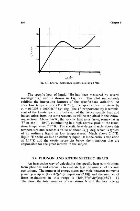
116

15~----+-----r---~-----+----~--~

Q 10~----~~~+---~~~-+~~-r--~ 2' ~ -" ;;.

5~--~+-----r---~-----+----~--~

0.-__ -. ____ .. __ -. ____ +-__ -+ __ ... o

pi"" (A-l)

Fig. 5.1. Energy-momentum spectrum in liquid 4He.

Chapter 5

The specific heat of liquid 4He has been measured by several investigators,6 and is shown in Fig. 5.2. This plot immediately exhibits the interesting features of the specific-heat variation. At very low temperatures (T < 0.6°K)" the specific heat is given by Cs = (0.0205 ± 0.OOO4)T3 J/g. deg. The T 3-proportionality is reminis­cent of the low-temperature behavior of the lattice specific heat and indeed arises from the same reasons, as will be explained in the follow­ing section. Above 0.6°K, the specific heat rises faster, somewhat as T6 or exp (- 10/T), culminating in a high narrow peak at the trans­ition temperature 2.17°K. The specific heat drops sharply above this temperature and reaches a value of about 3J/g· deg, which is typical of an ordinary liquid at low temperatures. Much above 2. 17°K, liquid 4He behaves like an ordinary liquid. It is the curious transition at 2.17°K and the exotic properties below the transition that are responsible for the great interest in the subject.

5.4. PHONON AND ROTON SPECIFIC HEATS

An instructive way of calculating the specific-heat contributions from phonons and rotons is to evaluate first the number of thermal excitations. The number of energy states per mole between momenta p and p + dp is (4n V /h3)p2 dp [equation (2.18)] and the number of Bose excitations in this range is (4nV/h3)p2 dp/[exp(e/kT) - It Therefore, the total number of excitations N and the total energy

Heat Capacity of Liquids 117

100

10

/ 'I V - -"

I V I I

I

2 / i

/ ~ [

3

10

4/ 10

0.2 0.4 0.6 0.8 1.0 2.0 3.0 4.0 5.0

Temperature (deg K)

Fig. 5.2. Specific heat of liquid 4He under its saturated vapor pressure. 6

E per mole are

41tVf p2 dp N = JI3 exp(B/kT) - 1

(5.4a)

41tVJ Bp2 dp E = JI3 exp(B/kT) - 1

(5.4b)

Consider first the case of phonons B = cpo The situation is the same as that occurring in the Debye theory of lattice heat capacity except that only longitudinal phonons are possible in the liquid state. The Debye temperature in the helium problem, obtained as usual by terminating g(v) at vD, is

() = he (181t2p)1/3 21tk mHe

(5.5)

and has a value of about 30°K. Therefore, regions up to 2°K may be considered as the Debye T3-region. In this low-temperature region no serious error is made in extending to infinity the integration in

118 Chapter 5

equation (5.4) over p/kT, and hence per mole

N_,,"" = 4nV(kTV foo x 2 dx = 4nV(kT)3 x 2.404 y •• v.. n' 3 ., "x 1 ,,3 r (5.6)

\C:/Jo" •.. ,-,

Ephon = 4~~C(k:J f~ e~3 ~x1 = 4~~C(k:y x ;;

The corresponding specific heat per gram is

16n5k4

cphm = 15h3c3p T3

(5.7)

(5.8)

For rotons, e = A + (p - Po)2/2/l. In practice, A/k is found to have a value of about lOoK; therefore, nothing is lost by using the simpler Maxwell-Boltzmann statistics, so that

N - 4nV r 2 d {- [A + (p - PO)2/2/l]} rol - YJP pexp kT

Further, the parameter Po in the helium problem is found to be much greater than /lkT, so that in the integration over dp the quantity p2 may be replaced by p~. Moreover, because of the rapid reduction of the exponential factor for large values of p - Po, the integration may be performed over p - Po from - 00 to 00. Thus per mole

4n V f"" 4n Vp2 Nrol = Yp~ e-l'1fkT _ qo e- x2 / 2I'kTdx = T(2n/lkT)1/2 e-fj,/kT (5.9)

A similar calculation gives the specific heat per gram as

Crol = ::3(~~y/2 p~A2 [1 + U; + i(U;J}-l'1fkT (5.10)

The temperature dependence of the roton part of the thermo­dynamic quantities is basically of the form exp( - A/kT~ This is a consequence of the finite energy gap A and the need for the Boltzmann­type excitation across the gap [compare equations (2.10) and (4.26H The number of phonons is proportional to T3, and a numerical esti­mate shows that below 0.6°K, practically all the excitations are of the phonon type. Around 0.7°K, the number of rotons overtakes the number of phonons; at temperatures above about 10 K, most of the excitations are of the roton type. Figures 5.2 and 5.3 show how the specific heat follows the gradual transition in the nature of the thermal excitations.

The phonon-type behavior at low temperatures is similar to the Debye T 3-region discussed in Chapter 2. As a matter of fact, if only

Heat Capacity of Liquids 119

lii',----------.---------.-------~'"

7 /'

., 10

/ / ...... ph

! / ......

I ...... ...... '3 ......

'" 10 ~

J r

., 10

., 10 ~_~~ ______ ~ ______________ ~-------------~,

1.0 1.5

---+ T(deg K)

Fig. 5.3. Specific heat of liquid 4He showing phonon and roton contributions.7

longitudinal phonons are present, equations (2.13) and (2.20) become

_ hC(~)1!3 () - k 4nV

16n5k4V 3

Cv=TI~T

and they are similar to equations (5.5) and (5.8). The velocity of sound in liquid 4He at low temperatures is 239 ± 2 M/sec. Equation (5.8) now gives C phon = (0.0204 ± 0.0005)T 3 Jig· deg, which is to be compared with the experimental value Cv = (0.0205 ± 0.OO(4)T 3

mentioned earlier. The excellent agreement provides strong support for the above picture of thermal excitations in liquid 4He at low temperatures.

Above 0.6°K, the roton contribution becomes significant; up to about 1.6°K, the specific heat can be accurately fitted by the addition of phonon and roton contributions. In 1947, Landau calculated the values of L1, Po, and f1 from such an analysis of specific-heat data (which at that time were not known with any great accuracy). A similar analysis was performed by Kramers and coworkers in 1956,

120 Chapter 5

Table 5.11. Comparison of the Values of ~, Po, and 11

~ f1<J(A-I) J1 I(degK) h m4He

Calorimetry Landau (1947) 9.6 2.0 0.77 Kramers (1956) 8.8 ± 0.1 1.96 ± 0.05 0.23 ± 0.1

Neutron scattering 1.1 oK 8.65 ± 0.04 1.92 ± 0.01 0.16 ± 0.01

using carefully determined values of specific heats. In Table 5.11 the numerical values of ~, Po, and J1 are compared with the results of neutron-scattering experiments in which the energy-momentum dispersion relation 5 was studied directly. The close agreement between the values must be taken as a striking vindication of Landau's calculation of the properties of liquid 4He on the basis of the special E-P relation (5.3).

Above 1.6°K, the number of rotons becomes so large that it is no longer possible to neglect the interactions among the excitations. (The analogy in the case of solids is the anharmonicity of lattice vibrations.) The neutron-scattering experiments show that the para­meter ~ changes slightly because of the interactions among the rotons. Taking into account the small temperature dependence of the para­meters and also using the full c-p curve, the Los Alamos group of workers8 has calculated the specific heats and find excellent agree­ment over the whole temperature range up to 2°K.

Finally, it must be added that the above picture of a gas of phonon and roton excitations accounts satisfactorily for a numbp.r of other properties of liquid 4He. A full account is given in the works cited earlier. 4.5

5.5. TRANSITION IN LIQUID 4He

It was the specific-heat measurement by Keesom and coworkers in 1932 that gave a definite indication of the special phase change in liquid helium at 2.1 rK. There is a sharp peak at 2.1 rK, and the shape of the curve (Fig. 5.2) resembles the Greek letter lambda (A). Phase transitions in which there is a similar sharp A-peak in the specific heat are now commonly called lambda-transitions; they are the result of cooperative effects in the system. A few other A-anomalies will be discussed in Chapter 7, while the thermodynamics of such phase changes is taken up in Chapter 8.

Heat Capacity of Liquids 121

The characteristic feature of the A-transitions in liquids and solids is the appearance of a sharp peak in the specific heat (and hence calorimetric measurements are frequently used to detect such transitions). It is obviously of interest to know whether the peak is a sharp maximum or really an infinite singularity with S C dT still remaining finite. The question assumes fundamental importance in the theoretical understanding of such transitions. On the one hand, approximate statistical calculations on reasonable models of sub­stances predict a finite maximum at the transition T;., the peak being rounded off in a temperature interval of about 10- 3°K near TJ.. in some calculations and there being a jump in the specific heat in other theories. On the other hand, exact calculations on highly simplified models predict that the specific heat has a logarithmic or other infinity, i.e., of the form C ~ constant x 10g1TJ.. - TI near T;. (see Section 4.6). No reliable guidance could be obtained from experi­ments on solids, owing to the difficulty of keeping the temperature constant throughout the specimen to within about 10- 6°K. Fairbank, Buckingham, and Kellers9 realized that a temperature resolution of about 10- 6°K was possible in liquid helium. It was also pointed out in the Introduction that thermal equilibrium occurs very quickly, in a few seconds at temperatures below around 4°K. These workers placed the liquid in intimate contact with copper fins and succeeded in measuring the specific heat to within a microdegree of the A-point.

In order to exhibit the nature of the specific heat very near TJ.. = 2.1 rK, the results are shown on successively expanded tem­perature scales in Fig. 5.4. The very large amount of expansion of each successive curve is vividly demonstrated by the fact that the width of the small vertical line directly above the origin indicates the fraction of the curve which is shown enlarged in the next curve on the right. The specific-heat curve maintains the same geometrical shape on all the expanded scales, and clearly there is no indication of any rounded maximum within 1O- 4 °K of TJ.., as suggested by some approximate theories. There was also no hysteresis between the values measured with increasing and decreasing temperatures.

The same data are plotted on a logarithmic scale in Fig. 5.5. On both sides of the A-point the data fall in two parallel straight lines over a factor of 104 in IT - TJ..I. The observations (in Jjg·degK) near the A-point are well fitted by the equation

c = 4.55 - 3.00 10gloiT - TJ..I - 5.2015 (5.11)

where 15 = 0 for T < Tic and b = 1 for T > T;..- The inclusion of a logarithmic term permits a simple representation of the specific heat

i "?

~ U

122 Chapter 5

24

22

~ 20

18

16

14

12

1O

~ 8

6

~ O~~-L~ __ L-~-L~-L~ __ L-~-L~-L~ __ L-~-L~ __ ~ - 1.5- 1.0- O.S 0 0.5 1.0 1.5 -4 -2 0 6 -20 - 10 0 10 20 30

I T -T~"II IT -T~lmd"V

Fig. 5.4. Specific heat of liquid 4 He near the A-point. 9 The solid lines represent equations (5.11) and (5.12). The width of the small line above the origin indicates the

fraction of the curve which is expanded in the next figure on the right.

in joules per gram of liquid helium up to about 3SK:

(-740) C = cD(T) + [130 - 90.9 log IT - TAil exp T

(-370) = cD(T) + [23.5 - 16.4 log IT - TAil exp T (5.12)

where cD(T) represents the Debye function, evaluated at each tem­perature with the appropriate value of density and velocity of sound.

Besides the specific heat, the thermal expansion coefficient also shows a logarithmic infinity as the A-point is approached, although measurements have been performed up to IT - TAl ~ 1O- 4°K only. It will be seen in Section 8.1 that the behaviors of the two quantities are interconnected and that

( TA)Cp = T;.(~l~) _ T;.(pA)(~P) (J T aT.l. p). p aT A

(5.13)

"i :' ~ J

Heat Capacity of Liquids 123

25

20

15

10

5

0 10 " 10-' 1 2

Fig. 5.5. Specific heat of liquid helium versus log IT - TJ9 Solid lines represent equations (5 .11) and (5.12).

Figure 5.6 shows a parametric plot of the specific heat and the expan­sion coefficient. 9 The straight line is the asymptotic value given by equation (5.13) with the experimental values of the various other quantities. The tendency of the observations to attain the limiting value is clear. Thus we must conclude that both the expansion coefficient and the specific heat are consistent with an infinite logarithmic singularity at T;..

At present, there is no complete theory of cooperative transitions. In special cases, as with magnetic transitions treated in Section 4.6, much progress has been made in expressing the thermodynamic quantities in powers of IT - T;.I. The outstanding observation of a logarithmic singularity in C p and f3 is an experimental property which must be explained by any proper statistical theory.

5.6. SPECIFIC HEAT OF LIQUID 3He

The ordinary liquid helium used in bulk is the isotope of mass 4. The isotope 3He is present to about 1 part in 107 in natural helium. However, since 1948, small quantities of 3He, produced by nuclear

124

i ."

~ "-

U

~ e

20

18

16

14

12

10

8

6

2

, =10-'-,

" - , _ 10-2 I

I

f I

? , ! ,

I

P-' ~ IO-I

" T<T), P , I

d , , ? , ,

I

r I :_,.10 ,

oL-~-i __ ~-L~ __ A--L~~~-L~L-~-L~

0.06 0.04 0.02 o - 0 .02 - 0.04 - 0.06 - 0.08

(p>./p)II

Chapter 5

Fig. 5.6. Cylindrical approximation near TJ.." Parametric plot of (TJT)C p versus (pJp)f3. Full line is the calculated asymptotic value.

reactions, have been available for research, and its use in cooling cryostats to approximately 0.3°K was mentioned in Chapter 1. Helium-three exists as a liquid even at OOK and becomes a solid only under a pressure of about 30 atm or more. It obeys Fermi-Dirac statistics, and the properties of liquid 3He are quite different from those of 4He. The experimental and theoretical evidence unequivo­cally points out that liquid 3He must be considered a Fermi system, whereas the superfluid properties of liquid 4He arise from the Bose-Einstein condensation. 5 Since 3He offers the possibility of studying a simple Fermi liquid, it has of late become the subject of an active field of study.ID.II

Heat Capacity of Liquids 125

The equations derived in Chapter 3 for an ideal Fermi~Dirac gas were initially considered as a convenient framework for describ­ing the properties of liquid 3He. For a F~D gas, the degeneracy temperature is

__ 1_('J.Nh3 )2/3 TF - 2mk 8 nV (5.14)

which for the density of liquid 3He has a value of about 5°K. Early measurements of nuclear susceptibility showed that XT was constant down to about 1.5°K, and the deviations at lower temperatures could be fitted to a perfect-gas model with a degeneracy temperature of about O.5°K, nearly ten times smaller than the expected value. In a simple-minded way, this could be explained by saying that the effective mass m* is about ten times the mass of the 3He atom. The measurements 12 of specific heat above O.5°K destroyed this naive

g, ."

" ~ ~

0 u

J'

Ie I

I I I

I I

" /

o~ __________ ~ ____________ +-__________ ~

o Temperature (deg K)

Fig. 5.7. Heat capacity of liquid 3He under its saturated vapor pressure (curve A).12 Curve B is the specific heat of F-D gas with TF = 5.00 K

and curve C is that with TF = O.5°K.

126

0.8

0.7

0.6

i 0.5

:' u

g ::::,. 0 .• 8 U

0.3

0.2

0.1 I I

I I

I

0

0

I I

I I

I

"

... . },;

/' . /

/

. ,'/ . .. ,.' I,' ~,'

f

0.1 0.2

T(deg K)

0.3

Fig. 5.8. Heat capacity of liquid JHe below O.4°K. 14

Chapter 5

0 ••

picture. The specific heat does not resemble, even qualitatively, the behavior of an ideal F- D gas with any value of m*. Figure 5.7 compares the specific heats of a F- D gas having TF = 5.0 or 0.5°K with the experimental results. (Strictly, Cv should be compared instead of C.at , but this does not improve matters. In fact, the devia­tions of Cv are equally serious. 13)

Below 0.2°K, the specific heat of the liquid does vary propor­tionally with T , as may be expected from the F- D gas relationship:

(5.15)

Any satisfaction at such simple behavior is, however, short-lived.

Heat Capacity of Liquids 127

The F-D theory also shows that if Yo is the magnetic moment per atom, the molar susceptibility X should tend to the value

X _ 4nmYo(3N)1/3 V-~nV

(5.16)

This functional relationship is obeyed very well, but quantitatively the agreement is very poor. The m* /m3He calculated from the specific­data has a value of about 2, that from susceptibility is about to, from compressibility data about 0.3, and so on. In other words, even though the F-D gas formulas give the correct temperature dependence at very low temperatures (~0.3°K), the observations are not con­sistent with the quantitative interrelationships among the various formulas.

5.7. LIQUID 3He AS A FERMI LIQUID

A solution to this dilemma at very low temperatures was sug­gested in 1956 by Landau; since then, the microscopic foundations of such theories have been intensely studied by Brueckner and others.5,ll According to Landau's theory of a Fermi liquid, the presence of strong interactions among the atoms renders a descrip­tion of the behavior of single particles meaningless and the statistical behavior is determined by the elementary excitations of the whole system. These excitations or quasi particles obey Fermi-Dirac statis­tics and may be taken as an effective description of an atom together with its polarization field caused by the correlated interactions. At low temperatures, the system may be visualized as made up of N quasiparticles of effective mass m*, but in calculating any physical property the fundamental quantity to be considered is the interaction function. Thus, in calculating the magnetic susceptibility, we must consider the dependence of the interaction function upon the nuclear orientations. In compressibility, the volume dependence of the inter­actions is involved. The specific heat is determined by the density of states at the Fermi level, and so on.

Detailed calculations show that the specific heat is given by equation (5.15) with m* instead of m. Therefore, from the experimental data, we can conclude that m*/m3He ~ 2. The expression for suscepti­bility involves besides m* the constants of the spin-dependent part of the interaction function. Thus a calculation of m* using (5.16) will not give the same effective mass as that calculated from specific­heat data. In this manner, the Fermi-liquid theory gives different

128 Chapter 5

interrelationships among the various properties of liquid 3He, although the temperature dependence is in many cases the same as that given by the F-D gas calculations. The details of the theory are unfortunately very complicated, and the mathematical techniques used in these many-body problems are not commonly known. Hence, it seems best to suggest suitable reviews5.15 for those interested rather than give a garbled version of the theory here. On the whole, the Fermi-liquid theory of the behavior of liquid 3He below O.2°K appears to be in reasonable accord with the experiments.

The situation at higher temperatures (T > OSK) is not very satisfactory. As seen from Fig. 5.7, the curve bears no resemblance to the variation expected for a F-D gas. A heuristic approach 13 has been to assume that the alignment of the nuclear spins gives a spin contribution (similar to the Schottky term discussed in Section 4.9) with a peak around O.3°K and that at high temperatures there are contributions from excitations not dependent upon the quantum statistics of the atoms. Such calculations have had quite some success in explaining thermal and magnetic properties. However, the concept of splitting the entropy into such contributions has been questioned by others as having no fundamental justification. Further, nothing is said about the origin of the assumed high-temperature contribu­tion, which is independent of the statistics. 11 On account of these factors, the calculations are not here discussed in any detail.

The electrons in a metal form another example of an interact­ing Fermi system, which has already been considered in Chapter 3. Several authors have conjectured that a phenomenon analogous to superconductivity of the electronic system (Sections 3.8 to 3.10) should occur in liquid 3He, also. The transition temperature cannot be calculated precisely, but is estimated to be approximately 1O- 3 °K, if not lower. One of the characteristics of the transition, which has been reviewed by Sessler5 • 1O, for example, is that the specific heat should exhibit an anomaly (Fig. 5.9) similar to the anomaly at the superconducting transition (Fig. 3.11). As mentioned earlier, phase transitions are best detected by specific-heat measurements, and so calorimetric measurements are being made to as low a temperature as possible. At the time of writing, Peshkov 16 has reported a small bump at O.OO55°K. Above 8 x 1O- 3°K, the specific heat increases linearly with T (Fig. 5.8), the value being given by Csat ~ 20T J/mole·deg. The evidence is not quite conclusive,17 but Peshkov's observations will constitute the discovery of an eagerly sought phase transition in liquid 3He~of course, by specific-heat studies!

One question which cannot be answered here is why although sound waves can be propagated through liquid 3He as through any

Heat Capacity of Liquids

° T ----Fig. 5.9. Predicted specific heat of the

superphase of liquid 3Hc.

129

other system, phonon terms are not included in the specific heat of liquid 3He. The answer lies deeply involved in quantum statistics. 18

Phonon-type thermal excitations obey Bose-Einstein statistics, whereas the system of 3He atoms obeys Fermi-Dirac statistics.

5.8. MIXTURES OF 4He AND 3He

Liquid 4He and 3He are completely miscible, except at low temperatures, where phase separation occurs for a range of concentra­tions. It has already been mentioned that the properties of mixtures are of considerable interest in chemical thermodynamics. 2,3 In the helium case, since the two pure liquids exhibit peculiar properties of their own, a study of the mixtures has special significance in quantum statistics. 19

Although considerations of space prohibit a detailed account of the various studies/o,2o one interesting result is worth mentioning. Taconis, Beenakker, and de Bruyn Ouboter5 have found that for dilute mixtures of 3He in liquid 4He, the specific heat at low tempera­tures « 1 OK) is nearly constant and equal to ~Rx per mole of the mixture where x is the mole fraction of 3He. This may be explained simply on the basis of an idea put forward by Pomeranchuk that in dilute solutions the 3He atoms do not interact with the superfluid 4He, and so form a gas of excitations. At low concentrations, the 3He atoms may be taken as nondegenerate and so will have a perfect­gas specific heat Cv = ~R per mole (as will be explained in Chapter 6). Therefore, the excess specific heat of the solution will be ~Rx per

130 ChapterS

mole of the mixture. Other properties, such as the velocity of sound, confirm this simple picture of the role of 3He atoms.

5.9. SUPERCOOLED LIQUIDS-GLASSES

When a liquid is cooled ordinarily, it solidifies into a crystalline state at its normal freezing point; however, some substances can be supercooled. A classic example is glycerine, which can be easily cooled below its normal freezing point of about 290°K. With some care in avoiding nucleation, the supercooled liquid can be taken right down to approximately OaK without any crystallization. At about 1'g "" l80oK, the behavior of glycerine changes from a liquid-like fluidity above 1'g to a solid-like rigidity below 1'g. The free energy of this solid is greater than that of the crystalline solid, but it represents a metastable thermodynamic state which can exist indefinitely under certain conditions. This highly supercooled liquid state is typical of most glasses; hence it is called the glassy state. The situation is thermodynamically the same with allotropes such as diamond, a metastable form of carbon.

The specific heat of glycerol has been measured by several workers and is summarized in the review on the glassy state by Davies and JonesY The heat capacity of the crystalline state [curve (a) in Fig. 5.10] is due to the vibrations of the molecules in the lattice, as analyzed in Chapter 2. The specific heat of the supercooled liquid [curve (b)] is considerably greater because of the additional complex motions possible in the liquid state. However, over a narrow interval of temperature around 1'g "" l80oK, the specific heat falls rapidly to a value just above that of the crystalline solid. Only a small dif­ference persists at lower temperatures. Similar marked decrease around 1'g is shown in the thermal-expansion coefficient, electrical conductivity, and other properties. It is an important characteristic of supercooled liquids that the viscosity increases by several orders of magnitude as the temperature is lowered through the transition region. In glycerine, it increases from about 106 poise at 1900 K to about 1013 poise at 1700K. Thus at about 170oK, the stress applied to maintain a strain relaxes to lie of its initial value in hours, com­pared to 10-3 sec at about 190oK, so that for practical purposes the substance behaves like a solid. Above 1'g, the molecules have all the mobility characteristic of liquids, but below 1'g they cannot change their configurations in any reasonable amount of time; the only other modes of motion are the lattice vibrations about their mean positions, as in a solid. This is the reason why the specific heat decreases sharply in the transition region.

Heat Capacity of Liquids

6()

50

g, 40 "0

~

~ ~ 30 8 -a. u

20

10

0

0 100 200 300

Temperature I deg K I

Fig. 5.10. Measured heat capacity of glycerine: (a) crystalline solid, (b) supercooled liquid,

(c) glassy state, (d) very slowly cooled liquid.

131

However, the glassy state is not a crystalline state. The viscosity increases so rapidly as the substance is cooled through 1'g that the spatial disorder of the liquid has been abruptly "frozen-in." X-ray diffraction studies22 confirm the molecular disorder in the glassy state. An interesting check is the calculation of the entropy dif­ference between the supercooled glass and the crystalline state (Fig. 5.11). At the melting point, the entropy difference, obtained from the latent heat, is about 15 cal/mole'deg, but below 1'g a dif­ference of about 5 units persists right down to OOK. This is a measure of the configurational entropy of glass which is "frozen-in" at 1'g. The persistence of such an entropy difference at OOK is not really a contradiction of the third law of thermodynamics,23 because the glassy state is not one of stable internal equilibrium. Suitable nuclea­tion can precipitate a crystallization of the whole system (devitrifica­tion of glass). Figure 5.11 shows that above 1'g the difference in entropy between the supercooled liquid and the crystal decreases rapidly with lowering temperature. At 1'g, however, the liquid

132

g, -0 . 1 :::" 3 a

~ ~ 0>

~ j! '" '0 >-0-

~ . ~ x

15

10

5

01-------+-----~~----~ o 100 200 300

T emperatutE' (dc') K)

Fig. 5.11. Excess entropy of the glassy solid over the crystalline state (full line). Curve d shows the excess entropy if the liquid is cooled

very slowly at T".

Chapter 5

becomes so viscous that configurational changes to lower the entropy do not take place in short periods of time. Oblad and Newton showed experimentally that if glycerine is kept undisturbed for a long time before the measurement is made at any temperature, the specific-heat curve appears as a smooth extension of the behavior above Tg [broken curves (d) in Figs. 5.10 and 5.11]. This shows clearly that if sufficient time (a whole week of undisturbed waiting just a few degrees below I'g) is allowed, molecular rearrangements do take place. Because of the experimental difficulties, measurements could be made to only a few degrees below I'g. Nevertheless, an inspection of Fig. 5.11 shows that the entropy difference will undoubtedly extrapolate to zero at oaK. If a liquid can exist in internal equilibrium, such as liquid 4He and 3He, its entropy will vanish at absolute zero.

The entropy difference between crystalline and glassy states is similar to the problem of entropy differences between the various

Heat Capacity of Liquids 133

allotropes of some solids. Materials such as sulfur, tin, and carbon exist in different crystalline states with different specific heats. An investigation of the entropy differences among them was originally used by Nernst and coworkers to check the validity of the third law of thermodynamics. With crystalline solids, it is, of course, possible to calculate the vibrational specific heats from suitable theoretical models. 24

Numerical values of the specific heat of glasses are of importance in practice, and Stevels22 has collected the data for a variety of glasses. Some cases of cryogenic interest are mentioned in Table 8.1.

REFERENCES

I. J. Frenkel, Kinetic Theory of Liquids, Dover, New York, 1954. 2. J. S. Rowlinson, Liquids and Liquid Mixtures, Butterworth, London, 1959. 3. E. A. Guggenheim, Mixtures, Clarendon, Oxford, 1952. 4. K. Mendelssohn, Handbuch der Physik, XV (2), 370 (1956). J. Wilks, Rept. Progr.

Phys. 20, 38 (1957). K. R. Atkins, Liquid Helium, Cambridge University Press, Cambridge, 1957.

5. Liquid Helium, Proceedings of the International Summer School "'Enrico Fermi," (Varenna, 1961, G. Careri, ed.), Academic, New York, 1963. J. Wilks, Liquid Helium, Clarendon, Oxford, 1966.

6. H. C. Kramers, J. Wasscher, and C. J. Gorter, Physica 18, 329 (1952). R. W. Hill and O. V. Lounasmaa, Phil. Mag. 2, 143 (1957). J. Wiebes, C. G. Niels-Hakken­berg, and H. C. Kramers, Physica 23, 625 (1957).

7. H. C. Kramers, Progr. Low Temp. Phys. 2, 59 (1957). 8. P. J. Bendt, R. D. Cowan, and J. L. Yarnell, Phys. Rev. 113, 1386 (1959). 9. M. J. Buckingham and W. M. Fairbank, Progr. Low Temp. Phys. 3, 80 (\961).

10. J. C. Daunt (ed.), Heliwn Three, Ohio State University Press, Columbus, 1960. II. E. R. Grilly and E. F. Hammel, Progr. Low Temp. Phys. 3,113 (\961). N. Bernades

and D. F. Brewer, Rev. Mod. Phys. 34, 190 (1962). D. F. Brewer, Progr. Cryo­genics 4,25 (1964).

12. G. de Vries and J. G. Daunt, Phys. Rev. 92, 1572 (1953); 93, 631 (1954). T. R. Roberts and S. G. Sydoriak, Phys. Rev. 93, 1418 (1954). D. W. Osborne, B. M. Abraham, and B. Weinstock, Phys. Rev. 94, 202 (1954).

13. L. Goldstein, Phys. Rev. 112, 1465 (1958). 14. D. F. Brewer, J. G. Daunt, and A. K. Sreedhar, Phys. Rev. IlS, 836 (1959). M.

Strongin, G. O. Zimmerman, and H. A. Fairbank, Phys. Rev. Letters, 6, 404 (1961). A. C. Anderson, G. F. Salinger, W. A. Steyert, and J. C. Wheatley, Phys. Rev. Letters 7,295 (1961).

15. A. A. Abrikosov and I. M. Khalatnikov, Rept. Progr. Phys. 22, 329 (1959). 16. V. P. Peshkov, Soviet Phys. JETP 19, 1023 (1964). 17. E. S. R. GopaJ, J. Sci. Indus. Res. 23,496 (1964). W. R. Abel, A. C. Anderson,

W. C. Black, and J. C. Wheatley, Phys. Rev. Letters 14,129 (1965). 18. K. Huang, Statistical Mechanics, Wiley, New York, 1963, pp.262, 384. 19. I. Prigogine, A. Bellemans, and V. Mathot, Molecular Theory of Solutions, North

Holland, Amsterdam, 1957, chapters 18 and 19. 20. J. 1. M. Beenakker and K. W. Taconis, Progr. Low Temp. Phys. 1, \08 (1955).

K. W. Taconis and R. de Bruyn Ouboter, Progr. Low Temp. Phys. 4, 38 (1964).

134 Cbapter 5

21. R. O. Davies and G. O. Jones, Advan. Phys. 2, 370 (1953). 22. J. M. Stevels, Handbuch der Physik. XIII. 510 (1962). 23. J. Wilks, Third Law of Thermodynamics. Oxford University Press, Oxford, 1961,

chapter 5. 24. F. Seitz, l,,/oderii Theory of Solids. ~Y1cGraw-HiH, l'!e\v York, 1940, chapter 14.

Chapter 6

Specific Heats of Gases

6.1. Cp AND Cv OF A GAS

The heat capacity of a gas depends strongly upon the conditions under which heating is done, whether at constant pressure or at con­stant volume. Indeed, it was pointed out in Chapter 1 that the ratio CJCv is as high as 1.67 for a monatomic gas. It is possible to measure directly both Cp and Cv in gases and vapors, and a representative list! of the values at 3000 K is given in Table 6.1. The specific heats refer to the "ideal" state of a gas at zero pressure and are calculated from the values at higher pressures by using a knowledge of the equation of state [see equation (1.17)]. Typically, at a pressure of 1 atm, Cp and Cv are higher than the "ideal" values by less than 1 % in the so-called permanent gases and by about 1 to 2 % in organic vapors.

The specific heat per gram is different for different gases. For heavy gases, the value of Cv is small, and for light gases, Cv is large.

Table 6.1. Molar Heat Capacities (in cal/mole.deg) at JOOoK and P = 0 atm

Gas

He A H2 N2 O2 CO NO HCI CI2

Cp 4.97 4.97 6.85 6.94 7.02 6.96 7.08 6.97 8.02 Cv 2.98 2.98 4.86 4.96 5.03 4.97 5.10 4.98 6.02 Cp - C,. 1.99 1.99 1.99 1.98 1.99 1.99 1.98 1.99 2.00

CO2 N20 S02 H2S NH3 CH4 C2H2 C2H4 C2H6

Cp 8.77 9.25 9.20 8.15 8.49 8.48 10.35 10.15 12.25 Cv 6.78 7.27 7.20 6.15 6.50 6.49 8.35 8.15 10.25 Cp - Cv 1.99 1.98 2.00 2.00 1.99 1.99 2.00 2.00 2.00

135

136 Chapter 6

The consideration of molar heat capacities provides a great simplifica­tion: Cv turns out to be about 3 caljmole'deg for monatomic gases (such as helium and argon) and about 5 cai/mole·deg for diatomic gases (such as H 2, N 2 , °2 , CO, NO, HCl). C p - Cv is approximately equal in all cases to 2 caljmole·deg. When it is recalled that the gas constant R has a value 1.987 in the same units, the difference between Cp and Cv is nothing other than equation (1.13):

Cp - C v = R

a relation first used by Mayer in 1842. Since the natural unit for the molar heat capacity is R, the striking feature of Table 6.1, demanding an immediate explanation, is that Ct, ~ ~R for monatomic gases and Cv ~ 1R for diatomic gases.

6.2. CLASSICAL THEORY OF Ct. OF GASES

Boltzmann's equipartition theorem is able to provide an ex­planation for the simple coefficients ~ and 1. This theorem, as ex­plained in Section 2.2, connects the internal energy of a system with its number of degrees of freedom (that is, the number of squared terms in the Hamiltonian function, which is the same as the number of independent coordinates required to describe the motion of the system). Each degree of freedom contributes tRT to the internal energy of a mole of the substance at thermal equilibrium. A mass point is a good model of the atoms in a monatomic gas, It has three translational degrees of freedom (Hamiltonian (p~ + p; + p;)/2m where the p are the momenta of the molecules), Therefore, the internal energy is E = 3 x tRT and Cv = 8E/8T = ~R, as is found to be the case. The molecules of a diatomic gas may be represented by a pair of masses rigidly connected together, i.e., a rigid dumbell. Then, besides having the three translatory motions, the molecules can rotate about any pair of directions perpendicular to its axis. There are altogether five degrees of freedom; consequently, E = 1RT and C v = 1R. Thus the specific heats of permanent gases are readily understood in classical statistics.

A closer study of Table 6.1 reveals, however, that this agreement between the equipartition law and the observed values is only limited. A linear triatomic molecule, such as CO2 or N 20, should behave like a diatomic molecule, because it can rotate only about the directions perpendicular to its axis. Therefore, Cv should be 1R, whereas the actual values for CO2 and N 20 exceed 1R quite significantly. A general polyatomic molecule which can rotate about all three principal axes should have Cv = ~R, which is also not the case. Even

Specific Heats of Gases 137

a diatomic molecule such as chlorine exceeds its equipartition value of Cv = tR.

The discrepancy is partly due to the fact that the molecules can have internal vibrations. Each mode of vibration has two square terms in the Hamiltonian, one for kinetic and one for potential energy, and so counts as two degrees of freedom. A diatomic molecule has one vibrational frequency, and a general polyatomic molecule has 3n - 6 vibrational modes. If the vibrational contributions are added, Cv = ~R ~ 7 caljmole'deg for diatomic gases and Cv = 3(n - l)R for polyatomic gases. (If the molecules of a polyatomic gas are linear, there are only 3n - 5 vibrations, and Cv is correspondingly less.) The specific heats in Table 6.1 are all less than this value. The vibrational heat capacity of polyatomic gases (and of chlorine) falls short of this equipartition value. Experiments made at higher temperatures (Table 6.11) revealed that at 2000a C H20, CO2, and S02 attain their equipartition value of 3(n - l)R ~ 12 cal/mole·deg, while N 2' °2, HCI, CO, and H2 are obviously moving toward their value of approximately 7 caljmole·deg. (Chlorine exceeds the equi­partition value because of anharmonicity and dissociation 1 ,2, both of which are not considered in this elementary account.)

Measurements at low temperatures revealed another short­coming of the classical theory. Eucken, as early as 1905, noticed that the heat capacity of hydrogen at liquid-nitrogen temperatures was significantly lower than the room-temperature value. Table 6.111 shows that Cv has become equal to about ~R below about 60a K. Cp decreases by the same amount (recall Cp - Cv = R), and the ratio CplCv goes from 1.40 at room temperature to 1.67 at soaK. The values below 60a K are typical of a monatomic gas, for which only translational degrees of freedom are possible.

The equipartition law provides no reasonable explanation for the observation that at low temperatures the vibrational and rotational degrees of freedom remain "frozen in" and begin to "thaw out" as the temperature is raised. The clarification came from the application

Table 6.11. Cv at High Temperatures (in cal/mole·deg)

Gas Temperature

(deg C) A N 2, O 2, H2 Cl2 H 2O CO2, S02 HCl,CO

0 2.98 4.98 4.90 5.90 5.93 6.90 500 2.98 5.35 5.29 6.30 6.95 9.43

2000 2.99 6.22 6.10 7.4 11.9 11.5

138 Chapter 6

Table 6.ill. Heat Capacities of Hydrogen (in cal/mole.deg)

Temperalufe (dcgK)

300 200 100 80 60 40

C v 4.86 4.49 3.42 3.18 3.05 3.00 CplCv 1.41 1.45 1.56 1.62 1.66 1.67

of quantum concepts to the problem. Inspired by Einstein's funda­mental resolution of the temperature variation of vibrational specific heat in 1907, Nernst suggested in 1911 the quantization of rotational and vibrational levels in gases. Hydrogen remained somewhat anomalous until Dennison suggested an explanation in 1927, following the earlier calculation of Hund. The advances made in quantum mechanics and spectroscopy after 1925 brought the theoretical calculation of thermodynamic properties of simple gases over wide ranges of temperatures to such a high degree of precision that it surpassed the accuracy of the experimental measurements.

6.3. QUANTUM THEORY OF Cv OF GASFS

It is qualitatively easy to see why the rotational and vibrational degrees of freedom are not fully excited at low temperatures. For the common molecules, the vibrational frequencies are in the range of about 1014/sec, and the associated energy levels have a spacing equivalent to hv/k '" lOoooK. So, at room temperature ('" 3000 K), only a few molecules have enough energy to excite the vibrational modes. The rotational frequencies are about 100 times smaller, so that at any temperature above lOOK the rotational modes are fully excited. The rotational energy levels in hydrogen are rather high because of the low moment of inertia of the molecule; therefore, hydrogen begins to contribute the rotational specific heat only above 60°K. The translation of these ideas into quantitative results is, of course, a standard problem in statistical mechanics. 3 •4 The present discussion is limited to some simple cases, which are nevertheless sufficient to illustrate the principles involved.

The simplest case to consider is a monatomic gas, schematically taken as a set of mass points with no interatomic forces. Let a large number of such atoms, each of mass m, be enclosed in a vessel of sides Lb L 2, L3 in which they obey the Schrodinger equation

V 2 tfJ + 8n2~E tfJ = 0 h

Specific Heats of Gases 139

for free particles of energy E. The wave functions should vanish at the walls, but because the number of particles N is very large in any physical system, the boundary conditions do not affect the final result (see also Section 2.5). It is therefore mathematically convenient to impose a periodic boundary condition, as in lattice dynamics,

t{t(x,y,z) = t{t(x ± Lt>Y,z) = .. , = t{t(x,y,z ± L 3)

so that the solutions can be taken as progressive waves instead of standing waves. The wave functions satisfying these conditions are

t{t = A exp[2ni(plx + P2Y + P3 Z)]

where Pi = hni/Li and ni are positive or negative integers. The energy of a molecule is e = (pi + p~ + p~)j2m The energy of the system is the sum of the energies of the particles, and so the final partition function of the system will involve the product of N terms each equal to

cO [-(Pi + d + P~)] Z = I exp

~=_~ 2mkT (6.1)

A simple calculation shows that the energy levels are approximately h2/2mkL2 ~ 1O-15°K apart, so that the summation over ni may be replaced by an integration over Pi:

VfII [-(Pi + p~ + P~)] Z = h3 exp 2mkT dpl dP2 dP3

Here V = LIL2L3 is the volume of the system. The integral from - 00 to 00 of e- x2 is well known to be n 1/2 , and so

Z = v(2n~kTr/2 (6.2)

The partitIOn function of the system Z would have been just the product of N such terms but for the fact that all the particles are indistinguishable. This means that

Z = ~!(Z)N (6.3)

because the N! ways of permuting the particles are indistinguishable from one another and must hence be counted as only one way. Therefore,

~ (2nmkT)3 /2] A = - kTln Z = - NkTln ( -h-z - + NkT In N - NkT (6.4)

140 Chapter 6

where Stirling's approximation In N! ~ N In N - N is used. It is now a simple matter to calculate

Ct. =~R (6.5)

The specific heat at constant volume is approximately 3 cal/mole'deg, as was borne out in Table 6.1. This value was also explained by the equipartition law, but the present calculations give the absolute value of the entropy at a pressure P = NkT/V as

S = -G;).. = R{i + In[(k~5/2 g(2:~r/2J} (6.6)

(Here a weight factor g, equal to 1 for structureless particles and equal to 2 for vapors of sodium, potassium, and thallium, which have doubly degenerate ground state, has been added for completeness.) This equation, first derived in a different manner by Sackur and Tetrode in 1912, is in excellent agreement with the experimental values of entropy determined calorimetrically (see Table 6.VII). As a matter of historic interest, Tetrode, from the calorimetric entropy of mercury vapor, obtained Planck's constant h to within 5 % of the accepted value.

6.4. ROT A TIONAL PARTITION FUNCTION

The power of statistical thermodynamics becomes obvious when the rotational degrees of freedom are considered. The simplest case is a heteronuclear molecule of moment of inertia I perpendicular to its axis. With spherical p'olar coordinates, the expression for the kinetic energy js !!T.= t/(l)2 + sin20cP2). The generalized momenta are Pe = a!!T /ae = Ie, P4> = a!!T /a cp = I sin20cp, and so the classical Hamiltonian is Yl' = (Pi + sin - 2 Op~)/2/. The transcription into quantum mechanical operators leads to the Schr6dinger equation

a2", 1 a2", 8n21E a02 + sin2 0 aljJ2 + ~'" = 0 (6.7)

The eigenfunctions of this equation are '" = p1ml(cos O)eim4>, with m = -j, -j + 1, ... ,j - l,j, where p1ml(cosO) are the associated Legendre functions. The energy levels are ej = j(j + 1)h2/8n 21, where j = 0, 1, .... Each energy level j possesses 2j + 1 independent wave functions and so must be assigned a weight 2j -+- 1. Proceeding as before, the partition function is

1 Z ='_(Z)N

N

2.5

2.0

@i " v 1.5 0 E ~

~

"2 1.0 :; v

0.5

o

Specific Heats of Gases 141

-./

V I

/ /

/ o 0.5 1.0 1.5 2.0

T/6r

Fig. 6.1. Rotational heat capacity of a gas of heteronuclear diatomic molecules.

where the partition function z for a single molecule is

00 [ V+ 1)eJ z = L (2j + 1) exp _ } r

j=O T (6.8)

where er = h2 18n2 Ik. Over the entire range of temperatures, the summation has to be carried out by numerical methods3 .4, and the rotational specific heat has the values shown in Fig. 6.1. Cv(rot.) has a simple form at high or low temperatures:

Cirot.) = R[1 + ls(iY + ... J (6.9)

(6.10)

The rotational heat capacity of diatomic molecules has the equiparti­tion value R ~ 2 cal/mole·deg at high temperatures. As the tempera­ture is lowered, Cv(rot.) attains a shallow maximum of about 1.1R at Tier ~ 0.8 and then drops down steeply. Below about Tier ~ 0.2, the rotational specific heat becomes too small to be resolved experi­mentally.

142 Chapter 6

Table 6.IV. Rotational Characteristic Temperatures Or of Gases (in deg K)

Gas

H2 HD HT D2 DT T2 HCl N2 O2 CO NH3

e, 85.4 65.7 58.4 43.0 36.5 29.1 15.2 2.86 2.07 2.77 12.3

Clearly, Or is the characteristic temperature governing the behavior of Cv(rot.). Now a study of the band spectra enables the moment of inertia of the molecules to be determined,5 and some values of Or calculated from such spectroscopic observations are given in Table 6.1Y. For most gases, Or is in the region where the substances would have become liquids or solids, and so in the gaseous state they have the limiting value of R, thus accounting for the success of the equipartition law. Only in the case of the light hydrogeneous molecules is there any possibility of observing the "freezing" of the rotational degrees of motion. Hydrogen and deuterium are specially treated below because of the additional interesting effects arising from nuclear symmetry in the molecules. The rotational heat capacity of hydrogen deuteride (HD), obtained by subtracting the translational contribution ~R from the observed heat capacity, is in good agree­ment with the theoretical curve of Fig. 6.1 if Or is taken as 65. rK. However, the observations are incomplete.

The treatment of polyatomic molecules is along similar lines, taking into account the possibility of rotation about all three axes and the molecular symmetry. For all polyatomic molecules, the equipartition value is reached in the gaseous state. The interest in the polyatomic gases is in calculating the entropy from the statistical partition function. The relevant formulas are analogous to the Sackur-Tetrode equation (6.6) and may be found in several treatises. 3 .4,6 A comparison of the statistical entropy with the experimental value often gives information about the ordered state of the solid. This will be taken up in Section 6.7.

6.5. HOMONUCLEAR MOLECULES-ISOTOPES OF HYDROGEN

The heat capacity of homonuclear molecules, of which H2 and D2 are of great interest,7 involves a consideration of the symmetry of the wave functions of the nuclei. Quantum mechanics shows that if the nuclei have an even mass number (for example, the deuteron), the wave function describing their motion must be symmetrical in

Specific Heats of Gases 143

nuclear coordinates, while if the nuclei have an odd mass number (for example, the proton) the wave functions must be antisymmetrical. Since the total wave function contains the product of the rotational and the nuclear spin functions, it is convenient to consider the two separately.

Interchanging the two nuclei of a diatomic molecule is equivalent to replacing fJ by IT - fJ and ¢ by IT + ¢ in the rotational eigenfunction pJml(cos fJ)eim<P, that is, replacing the ~unction by (-ltpJml( -cos fJ)eim<P, which is equal to (-1)1 pJml(cos fJ)e'm<P because pJml(cos fJ) is even or odd according to whether j + Iml is even or odd. Hence the molecular rotational function is symmetric in the nuclear coordinates for even values of j and anti symmetrical for odd j. It is convenient to write

Ze = j= 0~4 •.. (2j + 1) exp [ -j(j + 1)jJ

Zo = j= 1~5, .. (2j + 1) exp [- j(j + 1)~]

(6.11 )

(6.12)

If the nucleus has a spin I (in units of h), there will be orienta­tional quantization in an external magnetic field, with an eigenfunction for each of the P = 21 + 1 states. In the absence of a magnetic field, the orientated states become indistinguishable, but their number remains unaltered. Thus there are P spin wave functions t/lr(a), t/ls(b), where r, s = 1,2, ... , p, for each nucleus a, b of a homonuclear diatomic molecule. From them, there are 1P(P - 1) combinations of the type t/lr(a)t/ls(b) - t/lr(b)t/ls(a) (where r # s), which are antisymmetric in the nuclear coordinates, and there are 1P(P - 1) combinations of the type t/lr(a)t/ls(b) + t/lr(b)t/ls(a) (where r # s), symmetric in the nuclei, as well as P products t/lr(a)t/lr(b) also symmetric in the nuclei. In all, there are 1P(P - 1) antisymmetric and 1P(P + 1) symmetric spin wave functions of the molecule. These are the spin weight factors.

After these preliminaries, the rotational specific heat of hydrogen may be taken up. The hydrogen nucleus (proton spin I = 1, P = 2) has an odd mass, and so the total wave function must be anti­symmetric. This means that the symmetric rotational functions Ze

must be combined with the anti symmetric spin functions, while the antisymmetric rotational functions Zo are to be associated with the symmetric spin functions of degeneracy 1P(P + 1). If these weight factors 1P(P - 1) = 1, 1P(P + 1) = 3 are taken into account, the partition function for the equilibrium state of hydrogen becomes

144 Chapter 6

and the specific heat will be

d r 2 d J Cirot.) = dTLRT dT In (ze + 3zo) (6.13)

This formula, derived by Hund,8 did not agree with the measured specific heats of hydrogen if the spectroscopic value of the moment of inertia, 4.67 x 10- 40 g-cm 2 , was used.

The reason was very soon pointed out by Dennison. 9 The transitions between the states of different nuclear spins are due to the very small interaction of the nuclear magnetic moment with the magnetic field produced by the rotation. The normal hazards of molecular collision do not affect the nuclear spins, and so the transi­tions between the two states are extremely rare. Therefore, hydrogen normally behaves as if it were a metastable mixture of two entirely separate species of molecules-parahydrogen and orthohydrogen. In parahydrogen, the nuclear spins are antiparallel (resultant spin and magnetic moment of the molecule are zero), and so this anti symmetric spin state is associated with even rotational states. Orthohydrogen has the spins of the nuclei parallel and corresponds to odd rotational states. In normal hydrogen, the relative abundance of the two types of molecules will be determined by the equilibrium conditions at room temperature. Since at high temperatures, Zo is approximately equal to Ze, the relative abundance of para and ortho molecules will be in the ratio p-H 2: 0-H z = 1: 3. The specific heat of normal hydro­gen must be calculated by adding the contributions from the two species in this ratio, because during the course of an ordinary calorimetric measurement the ratio does not change appreciably. Thus

(6.14)

This formula is in excellent agreement with the observations on ordinary hydrogen (for which the usual abbreviation is n-H2)'

Although the transitions between the ortho and para forms of hydrogen are so infrequent that the mixture retains its room-tempera­ture composition of o-H2 :P-H2 = 3: 1 during normal measurements of the specific heat, it is possible to catalyze the transitions by bringing the gas into contact with activated charcoal or paramagnetic salts. Substances such as ferric hydroxide are commonly used as catalysts. The lowest energy state of the ortho molecule is the j = 1 state, unlike the para molecule with a zero-energy j = 0 state. So, at low temperatures the equilibrium gas contains mostly para molecules. Typically, equilibrium hydrogen contains 25 % P-H2 at 3()()OK and over 99 % p-Hz at 20°K. This almost pure para hydrogen, or any

e :; v

Specific Heats of Gases 145

50 100 150 200 250 JO() 350

Fig. 6.2. Rotational heat capacity of ortho, para, normal, and equilibrium hydrogen (8, = 85.4°K).

other mixture, will remain in metastable equilibrium if the temperature is changed in the absence of catalysts. Therefore, the specific heats of various ortho- para mixtures have been studied; the results are in excellent agreement with the theoretical calculations if Or is taken as 85.4°K. By selective adsorption of the ortho molecules on alumina, 99 % pure orthohydrogen has been prepared recentlylO and its properties studied.

The rotational specific heat of the various forms (ortho, para, normal, and equilibrium states) of hydrogen are shown in Fig. 6.2.

For deuterium, the nuclear spin I is 1, and so p = 3. Since the deuteron contains two particles (proton and neutron), the total wave function must be symmetrical. The even rotational functions Ze are to be coupled to even nuclear spin functions of weight tp(p + 1) = 6, while the antisymmetrical rotational functions Zo are to be associated with the antisymmetrical spin functions of weight tp(p - 1) = 3. So for a metastable mixture of deuterium (n-D 2 ),

6 d ( 2d ) 3 d ( 2d ) Cv(rot.) = 9 dT RT dT In ze + 9 dT RT dT In Zo (6.15)

! .

146 Chapter 6

The measurements on ordinary deuterium are in good agreement with th is rela ti on.

The para molecules have antiparallel nuclear spins. Therefore, paradeuterium is associated with odd rotational states, unlike para­hydrogen, which is associated with even j-states because of the difference in nuclear mass and hence symmetry. The temperature variation of CJrot.) for paradeuterium is thus similar to that of orthohydrogen. The specific heat of orthodeuterium resembles the behavior of parahydrogen in having a maximum in Cv(rot.), but because of the increased moment of inertia, the peak occurs at about 85°K in orthodeuterium as compared to about 1700K in para­hydrogen. Further, because of the higher percentage of even rotational states, normal deuterium shows a weak maximum in the specific heat at about lOO°K. The theoretical variation of CJrot.) shown in Fig. 6.3 is in good agreement with experiments if Or is taken as 43.0o K. At low temperatures, orthodeuterium is the more favored

J . O~---r----,-----.---""----.----r-----r---'

2 . S~---r-----~--~~-----+---~~---r---~---~

2.O+-_-+_--itj-~L_1---=~~¥~:t:== .. 1

f 1.5~----~~~-~~---+-----+---,~---~--~---1 -:-

1->

u 1.0~--~~-~~--~---~~---+---~--~--~

O~~-~~r--fl--r---~~---+----+----~--~--~

o~~"~--~p---~-----p----~----+---~~--" 25 50 75 100 125 150 175

Fig. 6.3. Rotational heat capacity of para, ortho. normal , and equilibrium deuterium (0, = 43.00 K).

Specific Heats of Gases 147

state, and so almost pure metastable orthodeuterium can be prepared for experimental studies. Enrichment of paradeuterium requires a special process. 1 0

Similar considerations apply to other cases such as that of CH4 ,

where the four hydrogen atoms are indistinguishable. However, these substances are no longer in the gaseous state when the deviations from the equipartition value are expected to arise. The study of tritium and its hydrides is barely possible. 11

6.6. VmRATIONAL AND ELECTRONIC SPECIFIC HEATS

The vibrational levels of molecules are 100 to 1000 times higher than the rotational levels; consequently, for many "permanent" gases the vibrational contribution becomes appreciable only at high temperatures. There are some substances, especially the organic vapors, which have rather low vibrational frequencies; for them, the vibrations are excited at room temperatures, as shown in Table 6.I.

The vibrational specific heat has been already calculated, in a different context. In Chapter 2, it was pointed out that a harmonic vibrator of frequency v has energy levels en = (n + !)hv, and so

z = I exp [_ (n + !)hV] = exp(!hv/kT) n=O kT 1 - exp(hv/kT)

Thus

. (ev)2 exp(ev/T) CiVlb.) = R T [exp(8v1T) - IF (6.16)

where 8v = hv/k. This is the well-known Einstein function [equation (2.9)], and the temperature variation of C v was represented in Fig. 2.1. (There is a small difference in that three-dimensional oscillators were considered in Chapter 2, whereas the present Cv(vib.) for the one­dimensional case is one-third the Cv considered in Section 2.4.) From spectroscopic studies of the vibrational frequencies, the values of 8v may be calculated, some of which are given in Table 6.V. For simple molecules, the vibrational specific heat is barely excited at

Table 6.V. Vibrational Characteristic Temperatures 8v (in 103 "1()

Gas

8v 6.0 5.3 4.3 4.1 3.7 3.1 3.4 2.2 0.80 0.46

148 Chapter 6

Table 6.VI. Vibrational Heat Capacity of Chlorine (in caljmole.deg)

Calculated Experimental

243

0.848 0.840

Temperature (deg K)

270

0.985 0.977

"" J17

1.188 1.148

391

1.407 1.459

452

1.530 1.557

3000 K, i.e., at about one-tenth ev ' Chlorine is an exception; the values, calculated from a band-spectrum value ofv = 16.95 x lOI2/sec, are compared with the experimental results! in Table 6.VI. There is indeed good agreement.

In polyatomic molecules, there are several vibrational frequencies, and the corresponding Einstein terms must be summed up. In many cases, to get full agreement with experiments, corrections have to be applied for the coupling between vibrational and rotational levels of the molecule and for the anharmonicity of the vibrations at higher temperatures. These problems are treated in several texts. 3 ,4

Electronic energy levels, being of the order of lO4°K apart, are not excited at room temperatures, In nitric oxide (NO) and a few free radicals, there are exceptionally low-lying levels with spacings of about 100oK, The excitations between such levels give rise to the Schottky type of specific heat (Section 4,9), Measurements in the gaseous state, which exists only at temperatures well above the specific-heat peak, are in reasonable accord with the calculations.4

6.7. CALORIMETRIC AND STATISTICAL ENTROPIES­DISORDER IN SOLID STATE

The study of the entropy of gases offers some interesting informa­tion about possible disorder in the solid state, which is of fundamental interest in connection with the third law of thermodynamics.!2 Statistical thermodynamics allows calculation of the absolute entropy of gases,1> as was outlined for the case of translational degrees of freedom. The expressions involve, besides the fundamental constants h, k, m, etc., the frequencies of rotational and vibrational modes and the possible degeneracy of the states of the gas. These quantities can be determined from spectroscopic observations, and the entropy can be calculated. 5 On the other hand, from the measured specific heats of the solid and liquid phases as well as the latent heats of the phase changes, it is easy to calculate the entropy of the gas at, say, the normal boiling point. The calorimetrically determined values must agree with the statistically calculated values, if the conceptions

Specific Heats of Gases 149

Table 6.VII. Statistical and Calorimetric Entropies (in cal/mole·deg)

Gas and boiling point (degK)

A Kr N2 CI 2 HCI HI CH4 C2H4 CO2 NH3 87.3 120.2 77.4 238.6 188.2 237.5 111.5 169.3 194.7 239.7

Statistical 30.87 34.65 36.42 51.55 41.45 47.8 36.61 47.35 47.55 44.10 Calorimetric 30.85 34.63 36.53 51.56 41.3 47.8 36.53 47.26 47.59 44.13

of the third law and the statistical mechanics of the substances are correct. Table 6.Vll, giving the relevant data at the boiling point of several simple substances, shows that the agreement is very good in most cases. This is indeed gratifying.

In some cases, calorimetric and statistical entropies do not agree so well as in Table 6. VII. Among the possible reasons for the dis­crepancy are (i) errors of calorimetry in the form of impure specimens, etc. ; (ii) anomalous variations of specific heat below the temperatures up to which measurements have been made, resulting in an incorrect extrapolation to OaK (compare Section 1.4); and (iii) inadequate knowledge of the molecular parameters or the equation of state. Even when these reasons are ruled out, differences between the statistical and calorimetric values persist in some cases. 13 Table 6.VIII shows that they are significantly greater than the limits of experi­mental error, which is of the order of ±O.l caljmole·deg in the unfavorable cases involving specific-heat anomalies in the solid state. Although at one time there was considerable discussion about these discrepancies, it is now settled that in these substances the solid phases are not in internal equilibrium. As in the case of glassy materials discussed in Section 5.9, the solid state contains "frozen-in" configurational disorder not revealed in the calorimetric measure­ments of specific heats and hence in the evaluation of the entropy. Whereas the statistical calculations give the entropy difference between the gas at its boiling point and a perfectly ordered state at OaK, calorimetry gives the entropy difference between the gas at its boiling point and a slightly disordered state at OaK. Therefore, the calorimetric values must be smaller than the statistically calculated results, which is in fact one of the salient features of Table 6.VIII.

Carbon monoxide is a molecule with quite similar atoms; in an ideal solid state, the atoms should be arranged in the perfect order ... CO CO CO CO .... A disordered state ... CO CO OC CO ... will have a slightly higher energy A, dependent upon the difference between C and 0 atoms. If the temperature T is much larger than A/k, fluctuations in thermal energy of the order of A/k are possible,

150 Chapter 6

Table 6. vm. Discrepancies Between Statistical and Calorimetric Entropies 13

Gas and boiling point (deg K)

CO N 20 CH 3 0 FCI03 S02F2 NO H 2O 0 20 83 184.6 99.7 226.5 217.8 121.4 298* 298*

Statistical 38.32 48.50 39.49 62.59 64.14 43.75 45.10 46.66 Calorimetric 37.2 47.36 36.72 60.17 62.66 43.03 44.28 45.89 Statistical-

Calorimetric 1.1 1.1 2.8 2.4 1.5 0.7 0.8 0.8

* H 2 0 and 0 20 at room temperature.

and the molecule rotates freely from the CO to OC configuration and back. At very low temperatures (T ~ !!.Ik), the solid will become completely ordered if allowed to do so. However, in any solid there are always intermolecular potential barriers b opposing the molecular motions. If these barriers are small compared to !!., an ordered state sets in at T ~ !!./k. If, however, the potential barriers are much larger than !!., then the high-temperature disordered state becomes frozen at T ~ blk. The ordering at lower temperatures is not possible, because the mismatch energy !!. is not sufficient to overcome the potential barrier b. If a molecule can take up one of two possible sites, the entropy of the frozen disorder is R In 2 per mole. The discrepancy in Table 6.VIII is 1.1 caJjmole·deg, which is slightly smaller than R In 2 ~ 1.38 units, suggesting that a part of the disorder had been removed before the potential barriers in the solid prevented any trend toward a perfect arrangement. Similar arguments apply to nitrous oxide. This is a linear molecule with the atoms nearly alike, so that its orientation in the solid state may be either NNO or ONN. The discrepancy, 1.1 units, is again a little smaller than R In 2. The same end-for-end disorder occurs in the long-chain l-olefins with more than eleven carbon atoms,14 while I-decene and smaller molecules are fully ordered in the solid state.

The magnitude of the difference in CH3D is about 2.7 call mole·deg, which immediately gives a clue to the nature of the dis­order. In a completely ordered state, the CH3D molecules may be expected to take up a position with the deuterium atoms in one particular site among the four tetrahedral carbon-hydrogen bonds. If the rotational motion has been frozen at relatively high tempera­tures, there will be a residual entropy of R In 4 ~ 2.75 units, which is very close to the experimental value. The same is the situation with the perchloryl fluoride FCI03, where the crystal fails to distinguish

Specific Heats of Gases 151

between the oxygen and the fluorine atoms in orienting the molecule in the solid state. There are four possible positions for the fluorine atoms, giving a disorder entropy R In 4 '" 2.75 units, which is close to the observed value of 2.42 units. In sulfuryl fluoride (S02F 2), the slightly asymmetric top molecules have two possible orientations in the solid state, resulting in an entropy difference of about 1.5 units.

The statistical entropy of nitric oxide is only 0.7 units higher than the calorimetric values. X-ray studies 15 show that nitric oxide is present as a dimer

~ .. Q O .. N

with nitrogen-oxygen bonds of 1.1 and 2.4 A, respectively. The X-ray diffraction patterns suggest that the dimer is distributed in the crystal without distinguishing between the corners occupied by the N atoms and those occupied by the 0 atoms. This randomness gives an entropy of R In 2 per mole of the dimer and so accounts for the ob­served difference tR In 2 '" 0.69 units per mole of the monomer NO.

Ice provides a celebrated example of a more complicated type of disorder which was first elucidated by Pauling. 16 In gaseous H 20, the HOH.angle is about 105°, and the two H atoms are at a distance of 0.95 A from the oxygen atom. In ice, the various molecules are bound together into a loose open structure by hydrogen bonds, and each 0 atom is surroun~ed by four other 0, tetrahedrally situated at a distance of 2.76 A. The water molecules retain their individuality to a large extent, but there is space only for one ~ atom along each tetrahedral 0-0 direction at a distance of 0.95 A from either oxygen. In a mole of ice there are 2N H atoms, and if there are two possible positions along each 0-0 bond, the possible number of configurations is 22N. Of these, only a few are acceptable. Consider any 0 atom and the available sites along the four tetrahedral direc­tions. There is one way of putting four hydrogens close to the 0 atom, giving {OH4)2+ ionic arrangement; there are four ways of getting (OH 3)+, six ways of getting (OH2 ), and four ways of getting (OH)-; and there is one way of getting (0)2 - ionic arrangement. Of these sixteen possibilities, only six yield the desired H 20 molecule; that is, only three-eighths of all possible configurations are acceptable to that 0 atom. Thus the total number of possible arrangements of a mole of the solid is (2)2N . (it = {!t. Therefore, the entropy asso­ciated with this is R In! = 0.81 caljmole·deg. This agrees very well with the difference of 0.8 units observed for both H 2 0 and D2 0. There is considerable evidence from neutron- and electron-diffraction studies for the essential correctness of the statistical disorder in ice, and the matter has been recently reviewed by Chidambaram. 1 7

152 Chapter 6

The hydrated sodium sulfate Na2S04 ·lOH20 shows a residual entropy of about 1.5 units, which has been explained on the basis of X-ray structural work 18 A four-member hydrogen-bonded ring exists in the structure, with the protons unsymmetrically located III the hydrogen bonds. Therefore, two arrangements,

H H H H "- / "- /

O-H ° ° H-O I I

H H other and other atoms atoms

H H I I

° H-O O-H 0 / "- / "-

H H H H

are possible, and a random population of the two schemes gives a disorder entropy of R In 2. Isomorphous Na2 Cr04 ·10H 20 has the same structure and presumably would have the same residual entropy.

It was mentioned earlier that if the mismatch energy A is much larger than the intermolecular potential barriers, an ordered state is achieved at a temperature T ~ A/k. Consider, for example, HI instead of CO. The atoms are so different that the energy difference A between HI and IH configurations is very large. Even at relatively high temperatures, there is insufficient thermal energy to permit such a disorder. As a matter of fact, such substances display the ordering process in spectacular specific-heat singularities, the typical example l9 of HI and DI being given in Fig. 6.4. These cooperative anomalies were first found in ammonium chloride by Simon in 1922 and have since been found in a large number of substances. They are discussed fully in the following chapter. The configurational entropy in these materials is removed at relatively high temperatures. Hence there should be no discrepancy between statistical and calorimetric entropies. The examples given in Table 6. VII confirm this.

6.S. HINDERED ROTATION

A molecule does not always rotate as a rigid body, as was implied in the calculations of Section 6.4. In many organic molecules, groups of atoms can rotate freely or partially about the bond directions. A classic example is the difference between ethane H3C-CH3 and dimethyl acetylene H3C-C=:C-CH3. In ethane, the influence of the hydrogen atoms of one methyl group can be felt by the other CH3

Specific Heats of Gases

30

2' " 24 . o E

.c, o ~ 18

I

"­U

12

6

o o

~ ~

01/ ~ l-\.. ,/' ~

/ ,/ V

-' -~......, '/ HI

~ /

",

30 60 90 120 150 180 210

Temperature (deg K)

Fig. 6.4. Heat capacities of HI and DI. 19

240

153

30

24

18

1 2 • o S

6 0

o

group, and so a rotation of one group about the C-C axis may be expected to have a potential of the form V = Vo (1 - cos 3¢). In dimethylacetylene, the CH3 groups are far away, and so the methyl groups experience little, if any, potential barrier for rotation about the C==C bond. In fact, the entropy calculated by assuming a free rotation of the methyl group agrees well with the calorimetric value in the case of this substance. On the other hand, the measured entropy of ethane falls between the entropies calculated by assuming free or no rotation about the C-C bond. It is clear that from such entropy differences a knowledge of the potential barriers may be obtained.

The hindered rotation of the radicals in a molecule can also be studied from infrared and microwave spectra of the substance. Wilson20 has recently reviewed the various methods of determining Vo. The thermodynamic method, though used first to obtain this information (mainly by Pitzer and his coworkers), is rather inaccurate because it depends upon the small difference between two large quantities, namely, the calorimetric entropy and the statistical con­tribution from translational, vibrational, and other modes. The

154 Chapter 6

spectroscopic determination is more accurate; Vo thus determined can be used to interpret the calorimetric data. Methyl chloroform is one of the early substances for which spectroscopic data made possible the satisfactory interpretation of specific-heat measurements. Methanol has been studied extensively by various methods, and the results are in very good agreement with one another. 4

6.9. ENTROPY OF HYDROGEN The entropy of hydrogen depends upon its composition. Johnston

and coworkers21 calculated the entropy of parahydrogen by using the measured specific heats up to 12°K and then making a Debye-type extrapolation of the heat capacity of the solid down to absolute zero. At the boiling point (20.76°K), the entropy comes out to be

1.0 .---,~-----------------,

0.9

0.8

0.7

74% 0.6

x

0.3

0.2

0.1

O~--~~=--L ____ ~ ____ ~ __ ~ ____ ~

2 4 6 8 10 12

T(deg K)

Fig. 6.5a. Heat capa­cities of mixtures of orthohydrogen and parahydrogen in the

solid state.

Specific Heats of Gases

Fig. 6.Sb. I.-peaks with ortho concentrations exceeding about 60 %.23 Curve (a) = 74 ~~ and curve (b) = 66 % orthohydro-

gen.

155

15

(0)

10

(b)

OL-____________ ~ ____________ ~

1.0 1.5 2.0

T(deg K)

14.8 ± 0.1 cal/mole·deg. The statistical entropy is easily calculated from the translational and rotational functions and a small vibrational partition function. The value 14.76 agrees very well with the calori­metric evaluation.

A similar statistical calculation of the entropy of normal hydrogen shows that it exceeds that of para hydrogen by 4.29 cal/mole·deg. This excess arises from three sources. Normal hydrogen is a mixture of orthohydrogen and parahydrogen in the ratio 0: p = 3: 1, and the entropy of mixing is equal to - R(t In t + i In i) - 1.14 units. A second source is the nuclear-spin entropy of orthohydrogen. The ortho molecules, with a resultant nuclear spin I = 1, have three possible orientations, and the degeneracy will not be revealed until the specific heats are measured down to about 1O- 6 °K. The excess entropy is R In 3 per mole of orthohydrogen, and so it contributes iR In 3 - 1.64 to the ordinary 3: 1 mixture.

A third contribution comes from the ordering of the rotational axes of the molecules at low temperatures. As mentioned earlier, ortho-para transitions take place only slowly in liquid and solid states, which makes it possible to measure the thermal properties of the condensed phases with various ortho-para concentrations.

156 Chapter 6

Such measurements were first performed by Simon, Mendelssohn, O':J,..,rl Dllha.."....r.Jn 22 ~n.rl 't"n" ... ., "'''(",~T'\tl'lT h'lT U~l1 ..... ""rl D;~1.r.a.t",_ ..... 23 .......... ..-l ...... 1.1.'-& .I.'\o.U.l.l'-'.l.U.UJ.J. U.l.lU lU.VI..'" J.v,",v.1.tli] LlJ .l..l.1.11 «..1.1U 1.'-1'"'1\.."'\'~Vl1 c:.L.11U

by Ahlers and Orttung.24 Measurements above helium temperatures (Fig. 6.5a) show that the specific heats of solid solutions of ortho­hydrogen considerably exceed those of pure parahydrogen. With ortho concentrations in excess of about 60%, the specific heat exhibits a pronounced i.-peak at about 2°K (Fig. 6.5b). The additional specific heat increases with increasing ortho concentration, and the entropy associated with the anomaly is only a little lower than R In 3 per mole of orthohydrogen.

The excess entropy is in fact what is expected. The ground state of the ortho-molecule is the j = 1 rotational state, which, because of the low moment of inertia, has considerable energy. Solid hydrogen has a very open structure, largely on account of the high zero-point energy; therefore, the potential barriers opposing rotation of the molecules are small. The ortho molecules may be rotating right down to O°K. The rotational level j = 1 is threefold degenerate, but since the molecular field in the solid is cubic and not spherical, different relative orientations have slightly differing energies of interaction. The lowest energy of the system occurs for an ordered arrangement of the axis of rotation; indeed, NMR experiments25 show that the ortho molecules become ordered in this way. The specific-heat anomaly is due to this cooperative ordering process, though recent investigations24 show that the details of the ordering process are more complicated than was originally supposed. It is evident that the removal of the threefold degeneracy gives an extra entropy R In 3 per mole of orthohydrogen, or ~R In 3 ~ 1.64 per mole of normal hydrogen. The sum of the three contributions (1.14 + 1.64 + 1.64 ~ 4.4 cal/mole·deg) is in satisfactory agreement with the calculated difference of 4.3 units.

A similar entropy contribution due to the removal of the three­fold degeneracy of para molecules is present in deuterium. Following the earlier experiments,26 which revealed anomalous specific heats similar to those shown in 6.5a, Grenier and White27 detected A-peaks (as in Fig. 6.5b) at about 3°K in the specific heat of solid deuterium, with para concentrations of more than approximately 65 %. They used a special enrichment procedure 1o to get para concentrations greater than the normal 33j %. Taking into account the various contributions, there is satisfactory agreement between calorimetric and statistical entropies.

REFERENCES

1. J. R. Partington and W. G. Shilling. The Specific Heats of Gases, Benn, London, 1924. A. Eucken, Handbuch der Experimental Physik, VIII(l) (1929), chapter 10.

Specific Heats of Gases 157

2. E. Justi, Spez!/ische Warme, Entropie, und Dissoziation technischer Gase, Springer, Berlin, 1938.

3. J. E. Mayer and M. G. Mayer, Statistical Mechanics. Wiley, New York, 1940, chapters 6, 7, and 8. J. G. Aston and 1. J. Fritz, Thermodynamics and Statistical Thermodynamics, Wiley, New York, 1959, chapters 18, 19, and 20.

4. J. S. Rowlinson, The Perfect Gas, Pergamon, Oxford, 1963, chapter 3. 5. G. Herzberg, Infrared and Raman Spectra of Polyatomic Molecules, Van Nostrand,

New York, 1945, p. 501; Spectra of Diatomic Molecules, Van Nostrand, New York, 1950, p. 466. K. S. Pitzer, Quantum Chemistry, Prentice-Hall, Englewood Cliffs, N.J., 1953, chapter 9.

6. L. S. Kassel, Chem. Rev. 18, 277 (1936). E. B. Wilson, Chem. Ret". 27, 17 (1940). 7. H. W. Woolley, R. B. Scott, and F. G. Brickwedde, J. Res. Nat. Bur. Std. 41, 379

(1948). 8. F. Hund, Z. Physik 42, 93 (\927). 9. D. M. Dennison, Proc. Roy. Soc. (London), Ser. A 115,483 (1927).

10. C. M. Cunningham, D. S. Chapin, and H. L. Johnston, J. Am. Chem. Soc. 80, 2382 (\ 958).

II. W. M. Jones, J. Chem. Phys. 16. 1077 (1948); 17, 1062 (1949). 12. J. Wilks, Third Law of Thermodynamics, Oxford University Press, Oxford, 1961,

chapter 5. 13. J. O. Clayton and W. F. Giauque. J. Am. Chern. Soc. 54, 2610 (1932). (Carbon

monoxide.) K. Clusius, Z. Elektrochem. 40, 99 (\934); R. W. Blue and W. F. Giauque, J. Am. Chem. Soc. 57, 991 (\935). (Nitrous oxide.) K. Clusius, L. Popp, and A. Frank, Physica 4, 1105 (1937). (Monodeutro methane.) J. K. Koehler and W. F. Giauque, J. Am. Chem. Soc. 80, 2659 (1958). (Perchloryl fluoride.) F. J. Bockoff, R. V. Petrella, and E. L. Pace, J. Chern. Phys. 32, 799 (1960); 36,3502 (1962). (Sulfuryl fluoride.) H. L. Johnston and W. F. Giauque. J. Arn. Chem. Soc. 51. 3194 (1929). (Nitric oxide.) W. F. Giauque and J. W. Stout, J. Am. CI,ern. Soc. 58, 1144 (1936). (Water.) E. A. Long and J. D. Kemp, J. Am. Chem. Soc. 58, 1829 (1936). (Heavy water.)

14. J. P. McCullough, H. L. Finke, M. E. Gross, J. F. Messerly, and G. Waddington, J. Phys. Chem. 61, 289 (1957).

15. W. J. Dulmage, E. A. Meyers, and W. N. Lipscomb, Acta cryst. 6,760 (\953). 16. L. Pauling, J. Am. Chem. Soc. 57, 2680 (1935); Nature of the Chemical Bond.

Cornell University Press, Ithaca, N.Y., 1960, p. 464. 17. R. Chidambaram, Acta cryst. 14, 467 (1961). 18. K. S. Pitzer and L. V. Coulter, J. Am. Chem. Soc. 60, 1310 (1938); G. Brodale and

W. F. Giauque, J. Am. Chem. Soc. SO, 2042 (1958). H. W. Ruben, D. H. Temple­ton, R. D. Rosenstein, and I. Olovsson, J. Am. Chem. Soc. 83, 820 (1961).

19. A. Eucken and E. Karwat, Z. phys. Chem. 112, 467 (1924). W. F. Giauque and R. Wiebe, J. Am. Chem. Soc. 51, 1441 (1929). K. Clusius and D. Wolf, Z. Natur­forsch. 2a, 495 (1947).

20. E. B. Wilson, Advan. Chem. Phys. 2, 367 (1959). 21. H. L. Johnston, J. T. Clarke, E. B. Rifkin, and E. C. Kerr, J. Am. Chem. Soc. 72,

3933 (1950). 22. K. Mendelssohn, M. Ruheman, and F. Simon, Z. phys. Chem. 815, 121 (1931). 23. R. W. Hill and B. W. A. Ricketson, Phil. Mag. 45, 277 (1954). 24. G. Ahlers and W. H. Orttung, Phys. Rev. 133, AI642 (1964). 25. J. Hatton and B. V. Rollin, Proc. Roy. Soc. (London), Ser. A 199, 222 (1949).

F. Reif and E. M. Purcell, Phys. Rev. 91, 631 (1953). T. Sugawara, Y. Masuda, T. Kanda, and E. Kanda, Sci. Rept. Res. Inst. Tohoku, Univ. A7, 67 (1955). G. W. Smith and R. N. Housley, Phys. Rev. 117, 732 (1960).

26. O. D. Gonzalez, D. White, and H. L. Johnston, J. Chem. Phys. 61, 773 (1957). 27. G. Grenier and D. White, J. Chern. Phys. 40,3015 (1964).

Chapter 7

Specific-Heat Anomalies

7.1. SPURIOUS AND GENUINE ANOMALIES

The idea that the specific heats of some materials show abnormal variations at certain temperatures was introduced as early as Chap­ter 1, and several examples of such uncommon behavior were men­tioned in Chapters 3 to 6. Before embarking upon a systematic classification of such unusual specific-heat variations, it is worthwhile to digress a little upon what constitutes anomalous behavior. Any definition of an anomaly is to some extent negative in that it invokes the standards for normal behavior, which obviously depend upon the progress of our knowledge concerning the thermal properties of physical systems. Thus, deviations from Einstein and Debye models of specific heats, at one time considered to be anomalous variations of specific heats, are now taken as normal in the light of detailed lattice calculations. Similarly, the unexpected behavior of the specific heat of a superconductor is now viewed as a simple consequence of the onset of superconductivity in the electronic system. The possi­bility always exists that the puzzles of one era may become clarified in the succeeding years. Consequently, it is best to adopt as a prag­matic simplification that, in most substances and in many simple theoretical models of solids, the specific heat decreases continuously as the temperature is lowered. If there is an increase associated with reduction of temperatures, giving in effect a maximum in the heat capacity, the behavior is generally called a specific-heat anomaly. Although at one time such events were rarely observed, they are now known to occur in numerous substances. In general, if the origin of the effect is known, we shall call a finite small maximum a peak in the heat capacity and a large, nearly infinite, maximum a singularity. It appears best to reserve the term anomaly for the cases where the explanation is unknown.

158

Specific-Heat Anomalies 159

It is useful to illustrate the above statements with some examples. For the majority of common solids, the typical low-temperature specific heat is that shown by the thick line in Fig. 7.1a, decreasing continuously to zero as OaK is approached. A few substances exhibit a definite maximum as shown in Fig. 7.1b, a specific-heat peak. A practical case, that of nickel sulfate at low temperatures, was shown in Fig. 4.11. Here, on the basis of theoretical and experimental studies of thermal and other properties, it was possible to resolve the observations into a lattice contribution and a Schottky term, as shown schematically in Fig. 7.1b. Much effort has gone into the resolution of experimentally determined total specific heats into simple

, -101

> v

Ie )

T-fbI

Fig. 7.1. (a) Typical specific-heat variation of many common solids (thick lines). Broken lines show a possible resolution into Debye and Schottky contributions. (b) Schematic picture of a specific heat peak. Broken lines show decomposition into lattice and Schottky contributions. (c) Frequency distribution for a combination of Debye and Schottky terms. The Schottky term is equivalent to removing frequencies at 2VE and

adding them at v" shown as shaded portions.

160 Chapter 7

lattice, electronic, and other contributions so that the anomalous part can be discussed independently. Unfortunately, this sort of decomposition game, played with numerical data, can be carried to extremes. It was noticed by Simon in 1930 that the specific heats of many solids could be fitted very well by a combination of a Debye and a Schottky term, somewhat as shown by the broken lines in Fig. 7.1a. It was then postulated that the lattice follows the Debye variation, while the electronic system follows the Schottky relation as a result of excitation between the ground state and a higher energy state. With several adjustable constants, the agreement in such cases is, as expected, very good.

The underlying physical reason for this kind of agreement is as follows. I A comparison of the Schottky equation (4.25) for the case go = gl with the Einstein equation (2.9) reveals that the Schottky term is the same as the difference Cv(TE/T) - Cv(2TdT) between two Einstein models with frequencies VE and 2vE. Thus, the above de­composition is equivalent to adding a number of frequencies at VE

and removing the same number at 2VE in the Debye spectrum. The resulting g(v) (thick line in Fig. 7.1c) has a slightly better resemblance to the actual frequency spectra of solids-compare Figs. 2.5 to 2.8-than a single Debye spectrum, and the better representation of the specific heats by such a frequency spectrum is not surprising. With other approximate representations of g(v), such as those attempted by Raman and coworkers, the situation is similar.

It is now natural to ask whether a Schottky term obtained by such a decomposition justifies considering the specific-heat variation to be anomalous. At present, such specific-heat contributions are not called anomalous. The Debye spectrum is now known beyond all doubts to be nothing more than a good approximation to the g(v) of solids; a judicious combination of Debye and other terms is at best a better approximation. Hence, any peak separated out from the observations is artificial and without proper theoretical justifica­tion; the actual specific heat can be represented equally well by an appropriate g(v), which can be studied and confirmed by other inde­pendent methods such as neutron-diffraction studies. It is only when there is an actual maximum in the observed total specific heat that the lattice and electronic modes are insufficient for an explana­tion. Therefore, a practical criterion for a specific-heat anomaly is the presence of a maximum in the temperature variation of specific heat.

It is thus clear that what could have been considered a specific­heat anomaly in, say, 1930 is now taken to be normal behavior of the lattice. Another way in which later studies establish the presence of normal behavior is in bringing to light insidious experimental errors.

Specific-Heat Anomalies 161

In particular, three sources of error in many early observations have been revealed. Where hydrogen or helium exchange gas is used to cool the specimen to low temperatures, the desorption of the gas at low temperatures vitiates calorimetric studies by preventing the easy attainment of good vacuum insulation and by causing liberation of the heat of desorption. Secondly, small amounts of impurities, especially of materials which have pronounced specific-heat peaks, often result in apparent anomalies. Magnetic materials showing transitions at low temperatures should be scrupulously avoided. Thirdly, uncertainties in temperature scales may cause errors in the evaluation of heat capacities. Several anomalies reported earlier in many common materials! have now proved to be results of these experimental shortcomings.

7.2. COOPERATIVE AND NONCOOPERATIVE ANOMALIES

In discussing the model systems which show specific-heat peaks it is convenient to start with a system of independent particles or modes. Indeed, the simple models of solids and gases in Chapters 2, 3, and 6 invoked only such independent modes of excitation, namely, independent phonons, electrons, and molecules. The simplicity of such a system is that the total energy is just the sum of the energies of the various independent modes. Since there is no mutual inter­dependence among the modes, the system is called a noncooperative one. Under these conditions, a rather complete theoretical analysis of the system is possible. The examples of Schottky effect (Section 4.9), rotational specific heat of gases (Section 4.5), and the heat capacity of some liquids and solutions2 show that even in these non­cooperative processes specific-heat maxima can occur. The practical examples of such peaks and their theoretical interpretation have been fully discussed elsewhere, and there is no need for further analysis in this chapter. As a matter of fact, the rotational specific heat of gases is so well understood that many authors do not classify its maximum as a specific-heat anomaly.

In some physical systems, the interactions among the constituents are so strong that the energy state of one constituent depends upon the energy states of its neighbors. For example, in a ferromagnet the probability of a given spin pointing along + Z is large if the nearby spins also point along + Z and small if they are aligned along - Z. Thus, the spin states are not mutually independent. The probability of transferring a particle to an excited state depends upon the degree to which the excited state is occupied. Under such conditions, the excited states are often too few until some critical mean energy, that is, some critical temperature, is approached. Then the process of

162 Chapter 7

excitation by mutual cooperative action takes over and the particles of the system are very rapidly transfered to the excited states in the vicinity of the transition temperature. Thus. the energy of the system is changed in a small interval of temperature. In consequence, the cooperative transition is revealed in the specific heat as a pronounced singularity at the transition temperature 7;,.

Several categories of cooperative phenomena are now known. The alignment of magnetic dipoles (spins), superconductivity of elec­tronic systems, superfluidity in liquid helium, order-disorder transi­tions, and the onset of molecular rotation are some topics mentioned earlier. The phenomenon of ferroelectricity is analogous to ferro­magnetism. There are other specific-heat singularities in rare-earth metals and at liquid-gas critical points. The present chapter will be concerned with these cooperative effects.

Specific-heat singularities due to magnetic interactions are by far the most frequent peaks observed at low temperatures. There are many ions which are paramagnetic; the presence of anyone of them in a substance gives rise to either noncooperative Schottky peaks or cooperative ordering singularities. In the latter case, the ordered state at low temperatures may be ferro-, ferri-, or antiferro­magnetic. Even in diamagnetic solids, the nuclear moments, if any, become ordered at sufficiently low temperatures. The experimental and theoretical aspects of these phenomena were discussed at some length in Chapter 4. Here it suffices to remark that if the spins become noncooperatively ordered, there is a smooth Schottky maximum, whereas in cooperative ordering the specific heat is probably infinite at the transition temperature 7;,. Where sufficiently careful measure­ments have been made, the specific heat shows a logarithmic infinity on the low-temperature side of 7;,. On the high-temperature side, it is not settled whether the singularity is logarithmic or of the power­law type.

Cooperative transitions in superconductors and superfluids were also fully discussed in earlier chapters. The two processes differ from the other cooperative phenomena in that the ordering takes place in the momentum space rather than in the coordinate space. F or instance, a ferromagnet becomes ordered with all spins along one direction in the ordinary coordinate space. On the other hand, the superfluid properties of liquid 4He are basically the result of Bose condensation of the particles into zero-momentum states. The Cooper pairs, which are responsible for superconductivity, behave very much like condensed bosons. There are, however, differences between the specific-heat behavior of superfluids and superconductors. Liquid 4He exhibits the famous A.-transition at 2.17°K, with the heat capacity showing logarithmic infinities both below and above T .. (Section 5.5).

Specific-Heat Anomalies 163

Superconductors show only a finite jump at the transition (Section 3.9). Further, liquid 4He has a specific-heat tail on the high-tempera­ture side of the transition, whereas at temperatures higher than 7;" superconductors give no clue about their dramatic properties below the transition. There have been suggestions that superconductors should also exhibit ),-type singularities, but careful experiments have up to now failed to reveal any such behavior. 3 The transition in liquid 3He, if confirmed, should prove very interesting. Several authors have predicted a peculiar anisotropic state of the liquid below 7;,.

With a variety of known cooperative effects, obviously no general theory of such processes can be given, and each effect is best treated on its own merits. Thereafter, it will be appropriate to show how co­operative phenomena can be interpreted in terms of simple models.

7.3. ORDER-DISORDER TRANSITIONS

In an ordinary alloy, the atoms are distributed at random over the available lattice sites. As the temperature is lowered, the third law of thermodynamics predicts that an ordered state having less entropy should result. However, in many cases the random arrange­ment is forcibly preserved by the interatomic potential barriers preventing the free movement of atoms. An illustration would be a typical tin-lead solder. This freezing-in of disorder has been men­tioned earlier (Sections 5.9 and 6.7). In other cases, the material lowers its entropy by precipitating individual grains of the component pure metals. In a few cases, the alloy (say AmBn of metals A and B) lowers its entropy by taking up a structure appropriate to a crystal­line chemical compound AmBn. This last transformation is the one under consideration here.

A classic example is the alloy f1-brass, CuZn. At or below room temperature, the substance has perfect cubic symmetry. The Zn atoms occupy the comers of a cubic unit cell, and the Cu atoms occupy the cube center. Thus, in this state f1-brass may be visualized as two interpenetrating simple cubic lattices of Cu and Zn. At a temperature of about lOOooK, the structure is disordered in the sense that the Cu and Zn atoms occupy sites at random. As the tempera­ture is raised from OOK, the ordered state (schematically shown in Fig. 7.2a) is gradually transformed into the disordered state (shown in Fig. 7.2b), although the process occurs very rapidly in the vicinity of the transition temperature 7;, ~ 469°C. The change in lattice structure is most easily followed by X-ray or neutron scattering. Many alloys, among them AuCu, AuCu 3, CuPt, and AgZn, show order-disorder transformations.4

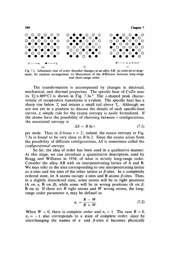
164

000 0 0 0 • • • • • 000 0 0 0 • • • • • o 000 0 0 • • • • • 000 0 0 0 • • • • • O--A .--B

(0)

o • • 000 • • • 0 • o • • 0 0 0 • • 0 • 0 o 0 0 0 0 0 00. • •

• 0 0 0 • 0 • • 0 • •

(b\

Chapter 7

o • 0 0 • 0 • • 0 • 0 o 0 • 0 0 0 • 0 0 • • • 0 0 0 0 0 o • • • 0

000 0 • 0 • • • • 0 @-- A or 8 atom

(c\

Fig. 7.2. Schematic view of order-disorder changes in an alloy AB: (a) ordered arrange­ment, (b) random arrangement, (c) illustration of the difference between long-range

and short-range order.

The transformation is accompanied by changes in electrical, mechanical, and thermal properties. The specific heat of CuZn near its 7;,( ~ 469°C) is shown in Fig. 7.3a. 5 The A-shaped peak charac­teristic of cooperative transitions is evident. The specific heat has a sharp rise below 7;, and retains a small tail above 7;,. Although we are not yet in a position to discuss the details of such specific-heat curves, a simple rule for the excess entropy is easily formulated. If the atoms have the possibility of choosing between r configurations, the associated entropy is

AS = R In r (7.1)

per mole. Thus in f3-brass r = 2; indeed, the excess entropy in Fig. 7.3a is found to be very close to R In 2. Since the excess arises from the possibility of different configurations, AS is sometimes called the configurational entropy.

So far, the idea of order has been used in a qualitative manner. At this stage, we can introduce a quantitative description, used by Bragg and Williams in 1934, of what is strictly long-range order. Consider the alloy AB with an interpenetrating lattice of A and B. We may refer to the sites corresponding to one interpenetrating lattice as a-sites and the sites of the other lattice as f3-sites. In a completely ordered state, let A atoms occupy a-sites and B atoms f3-sites. Then, in a slightly disordered state, some atoms will be in right positions (A on a, B on f3), while some will be in wrong positions (A on f3, B on a). If there are R right atoms and W wrong atoms, the long­range order parameter (5/ may be defined as

R-W (51=R+W (7.2)

When W = 0, there is complete order and (5/ = 1. The case R = 0, (5/ = -1 also corresponds to a state of complete order, since by interchanging the names of a- and f3-sites it becomes physically

Specific-Heat Anomalies

0.25

0.20

~ -u

'" :::0-S

0.1 5

uCl.

0.1 0 r~

100

v 0; E o o Cl.

~

~

o

J

V J

V .,/ ---

200 300 400

Temperature (deg C)

(a)

-

T/Tc _

(b)

\

~

- ---500 600

\ as

01 "

165

Fig. 7.3. (a) Specific heat of CuZn. 5 (b) Temperature variation of order parameters.

166 Chapter 7

identical to the case W = O. Complete disorder exists when there are as many right atoms as wrong ones, that is, when R = Wand (J"/ = O. Therefore, only the range between (J"/ = 1 (complete order) and (J"/ = 0 (complete disorder) is of physical interest. At very low tem­peratures, (J"/ is unity, and it drops rapidly to zero when T.: is reached, as represented in Fig. 7.3b.

The short-range order parameter (J"s may also be easily intro­duced, following the work of Bethe in 1935. In many systems, the interaction among the atoms is significant only for the nearest neigh­bors. For instance, the spin exchange integrals of Section 4.6 are nearest-neighbor interactions. Therefore, as a criterion of order we may compare the number of right pairs (AB type) and the number of wrong (AA or BB) pairs of near neighbors. An illustration will clarify this concept. From the point of view of long-range order defined by equation (7.2), the lattice of Fig. 7.2c is highly disordered. Yet nearly all atoms have unlike atoms as nearest neighbors. So if the relative number of right and wrong neighbors is taken as a measure of the ordering in the vicinity of any atom, the lattice is only slightly disordered. Consider an A atom. Let the probability that a given neighbor is a B atom be (l + (J"s)/2 and the probability that it is an A atom be (1 - (J"s)/2. For complete order (J"s = 1 and for complete disorder (J"s = O. Therefore, (J"s is called the short-range order para­meter. The temperature variation of (J"s is shown schematically in Fig. 7.3b. As T.: is approached, (J"s decreases rapidly from unity, but even above T.: short-range order persists for some temperatures.

7.4. ONSET OF MOLECULAR ROTATION

The nature of atomic motions in solids is obviously controlled by the interatomic forces. In rocksaIt, the Na + ions are equally strongly bound to the six surrounding CI- atoms, and it is hard to identify a single NaCI molecule or the molecular frequencies. If the intramolecular forces are comparable to the intermolecular forces, it is sometimes possible to identify distorted motions of parts of the molecules, for example, the C03 vibrations in solid CaC03.

In the extreme case of loosely bonded molecules, the molecular motions are practically unaffected at high temperatures; it was men­tioned in Section 6.7 that under such circumstances the molecules or radicals may be freely rotating. Consider as an example solid methane, in which the spherical CH4 molecules are loosely held together by Van der Waals forces. The methane molecules are freely rotating at "high" temperatures. On reducing the energy content of the solid by cooling it to "low" temperatures, the rotational motion is found to die down in a cooperative way. The specific heat of methane,6

Specific-Heat Anomalies 167

12

10

I ~

/ ~ /

~ /

o 10 20 30 40

Temperature (deg K)

Fig. 7.4. Heat capacity of methane."

given in Fig. 7.4, shows the familiar A-peak. Structural studies,7 in particular those in which magnetic resonance and neutron diffrac­tion were used, reveal that the CH4 molecules are freely rotating above ~ = 200K. At lower temperatures, they perform hindered rotations or torsional oscillations backward and forward about a mean position.

The transition in solid hydrogen, treated in Section 6.9, is another well-known example of a cooperative onset of molecular rotation. In orthohydrogen, the axis of rotation, which is not unique above ~, becomes ordered below the transition. Similar specific­heat singularities in hydrogen halides and in various ammonium salts were mentioned in Section 6.7. As a matter of fact, the specific­heat singularity in solid NH4 Cl, observed by Simon in 1922, was the first true A-anomaly to be discovered. In many cases, the precise nature of molecular rotations is not yet clear, and the available evidence suggests that they differ from substance to substance. However, a discussion of the various individual cases 7 is not appro­priate here.

7.5. FERROELECTRICITY

Solids belonging to ten of the thirty-two crystallographic classes lack inversion symmetry. They can exhibit electric polarization in the absence of an electric field, owing to the spontaneous alignment

168 Chapter 7

of electric dipoles. In contrast to the magnetic case, this electric polarization cannot be observed under ordinary static conditions, because it is compensated by free charges on the surfaces. However, the polarization is temperature-dependent, and so changes in it can be deduced from the current flowing in a closed circuit when the temperature of the crystal is changed. For this reason, substances belonging to the ten noncentrosymmetric classes are called pyro­electric.

Some pyroelectrics have the additional property that the spon­taneous polarization can be reversed in sense by an applied electric field. The material is then said to be ferroelectric. Thus, in ferro­electrics the polarization can be measured simply by reversing the applied electric field. In nonferroelectric pyroelectrics, dielectric breakdown occurs well before a field large enough to reverse the polarization can be applied. The dielectric behavior of a ferroelectric is complex. Not only is the relation between the polarization P and the applied field E nonlinear, but there is also a hysteresis loop, analogous to the ferromagnetic case. The alignment of the dipoles is opposed by thermal agitation. On increasing the temperature, the ordering is disturbed, and at a critical temperature, the ferroelectric Curie point, it breaks up. The crystal loses its ferroelectricity and becomes an ordinary dielectric (paraelectric state). Rochelle salt, ammonium dihydrogen phosphate, barium titanate, and triglycine sulfate are among the well-known ferroelectrics. There are several excellent reviews of this field. 8

The onset of ferroelectric ordering gives rise to A-type peaks in the heat capacity. The behavior of potassium dihydrogen phosphate (KDP), which is ferroelectric below 123°K, is typical of the specific­heat studies. 9 Superimposed on the usual lattice contribution is the configurational specific heat associated with ferroelectric ordering at 123°K (Fig. 7.5). The detailed behavior near the Curie point is slightly uncertain in most ferroelectrics because of the existence of thermal hysteresis; that is, the specific heat on cooling is slightly different from that on warming. The entropy associated with the excess specific heat is about 0.7 cal/mole·deg, which is close to the value t R In 2. The spontaneous polarization p. decreases slowly as the temperature is raised from OaK, but drops rapidly as 1'.: is approached. Just as in the magnetic case [equation (4.17)], the excess specific heat should be proportional to dP;/dT. This relationship is approximately obeyed in KDP. 10 Further, there is evidence10a that the specific heat near T.: may be fitted to logarithmic singularities, of the type discussed in Sections 4.6 and 4.7.

The similarity between ferroelectricity and ferromagnetism extends to other forms of ordering as well. Ferroelectricity and

t 0

-0 E

0

a. U

Specific-Heat Anomalies

36

32

28

2'

20

16

12

)

L V

/' ,r

/ ~V

20 40 60 80 100

120

T emperohJl"e (deg K)

~ V--

---

140 ISO 160

Fig. 7.5. Heat capacity of KH 2 P04 . 9

169

..,.,....,..

200

antiferroelectricity are also known; these topics are discussed in the many reviews on the subject.8 In spite of these similarities, the molec­ular basis of the electric phenomenon is apparently very different. Tak­ing the example of KH 2P04 , the deuterated KD2 P04 has a transition temperature ('" 213°K) nearly double that of KDP. Yet the entropy associated with the transition is nearly the same in the two salts. The entropy excess suggests some form of order-disorder process, while the dependence on the mass of hydrogen shows that the hydro­gen atoms are involved in the ordering. Indeed, the theoretical ex­planations of ferroelectricity, originally advanced by Mueller, Slater, and others, invoke an ordering of the hydrogen bonds. For a large number of compounds, order-disorder structures of the hydrogen bonds are possible. 8 In ionic ferroelectrics such as BaTi03 , another mechanism has been suggested by Anderson, Cochran, and others. 11

This is based on the idea that in an optical mode (Section 2.8) the

170 Chapter 7

adjacent charges vibrate out of phase. If the restoring forces and hence the frequency tend to zero, a spontaneous separation of charges, which is nothing but the spontaneous polarization under considera­tion here, is possible. Thus, it is suggested that as the temperature is lowered the frequency of some optical mode decreases rapidly and becomes zero at~. Such a mechanism, which is supported by neutron­diffraction studies on SrTi03, explains many observations on BaTi03-type ferroelectrics. These questions are treated at length in the reviews already cited.

7.6. TRANSITIONS IN RARE-EARTH METALS

The rare-earth metals, lanthanum (atomic number Z = 57) to lutetium (Z = 71), can be isolated and purified only with some special techniques developed in the last twenty years. Much of the work done before 1950 was on impure metals; as seen earlier, the impurities often have very disturbing effects on specific heats. Recent studies12 on relatively pure metals have shown very complicated thermal and magnetic properties. The rare-earth metals show unusual types of ferro- and antiferromagnetic orderings13 which give rise to these complicated phenomena. Thus, a discussion of the heat capacity of rare-earth metals should belong to Chapter 4. However, on account of the variety of abnormal effects observed and the very large gaps in our knowledge, these matters are considered here.

The electronic structure of the rare-earth metals may be written as Xe core-4fn; 5s2 , 5p6; 6s2 , 5d1-although some exchange between the 4 f; and 5d-shells takes place. As the atomic number Z increases from 57 to 71, n increases from 0 to 14. The 4fshells are largely screened by the closed 5s- and 5p-shells, so that magnetic and Stark interactions are weak. As a result of the subtle balance between these interactions and the normal thermal energy, the metals show very complicated thermal, magnetic, and other properties. A brief account of the specific-heat behavior will highlight the challenging problems in the study of these metals.

Lanthanum (Z = 57, n = 0) has no 4 f-electron, is a super­conductor, and behaves in a normal way.

Cerium has one 4f-electron and exhibits the complex specific-heat behavior shown in Fig. 7.6. As the specimen is cooled from room temperature, the specific heat follows the curve A in the region 200 > T > 120°K. On warming from a low temperature, the specific heat follows the curve B, exhibiting a pronounced thermal hysteresis. Some latent heat is also evolved in the region L around 100°K. At 13°K, there is a large peak in the specific heat, which is due to the onset of antiferromagnetism at lower temperatures. At about 200oK,

Specific-Heat Anomalies

-0-U

i 20 40

V It v v

J: I I(~

60

V

."

20 40 60

80 100 120 140 '/l 180

B .. / ~,. Y '\

~ l ,/ Ce

~ t-:.

-~

80 100 120 1040 160 180

Temperature (deg K)

Fig. 7.6. Heat capacities of cerium and neodymium. 14

200

• 200

10

171

0-V

the fcc lattice of cerium starts to undergo a transition into a com­pressed fcc' lattice of about 15 % less volume. Besides the fcc' phase, there is another hcp phase at low temperatures. 1 5 Apparently the fcc;: fcc' transition is an electronic one in which the magnetic 4 [electron goes over into the 5d conduction band. These phase changes involve very little rearrangement of atoms and show a pro­nounced dependence upon the stresses and strains in the crystal, past thermal history, and the state of crystalline imperfections. Thus, on repeated cooling to 200K and warming to 300oK, the hysteresis loop at 1600 K collapses and the peak at 13°K is enhanced. Such a sluggish dependence upon thermal history is characteristic of martensitic transformations,16 of which another example, namely, that of sodium, was mentioned in Section 2.10. At the present time, however, there is no quantitative explanation of the hysteresis effects.

Praseodymium has a large specific-heat bump distributed around 400 K. Neodymium (Z = 60) has two peaks, one at gOK and another at 19°K (Fig. 7.6). Below gOK, there is an ordering into the ordinary

172 Chapter 7

antiferromagnetic state discussed in Section 4.2. The peak at 19°K is due to the onset of a special type of antiferromagnetism, which will be mentioned later (Fig. 7.8e). The peak in praseodymium also arises from a similar special type of antiferromagnetic ordering. 1 7

The heat capacity of promethium, an element which has to be produced artificially, has not been studied so far. Samarium (Z = 62) has a sharp singularity at 15°K due to antiferromagnetic ordering. There is a second peak at 106°K, but as yet no corresponding anomaly in the magnetic behavior has been found. Europium is antiferro­magnetic below about 90 0 K.

The ferromagnetism of gadolinium below 289°K is very well known. The specific heat has a large A-singularity at that temperature (Fig. 7.7). The next five metals, in which n runs from 8 to 12, show complex ferro- and antiferromagnetic states. Terbium is paramagnetic down to 230oK, where it becomes ferromagnetic. Dysprosium (Fig. 7.7) is paramagnetic down to 175°K, when it becomes antiferro­magnetic, and then at 85°K it becomes ferromagnetic. There is a large A-peak at 175°K and a symmetrical peak at 85°K. Holmium behaves in a similar manner, with a A-peak at the Neel point (132°K) and a symmetrical peak at the ferromagnetic Curie point of 20oK. In between the two temperatures, the specific heat rises rather non­uniformly, a feature which is aggravated in erbium (Fig. 7.7). Between its Neel point of 80 0 K and its Curie point of 19°K, there is a rounded maximum at 54°K, just discernible in the scale of Fig. 7.7. This arises from complications in magnetic ordering, which are discussed below. Thulium becomes antiferromagnetic on cooling to 15°K. With these metals, the specific heat at the ferromagnetic transition shows con­siderable hysteresis.

In yttrium (Z = 70), the 5d-electron goes into the 4fshell, which otherwise should have n = 13, and completes it. Therefore, the metal does not exhibit any striking magnetic or thermal phenomena. Like­wise, lutetium, which has a closed shell (n = 14) of 4felectrons, behaves normally.

Even this sketchy summary is enough to show that nearly every type of specific-heat abnormality' is present in these metals. This complex behavior corresponds to the complicated magnetic structure, which is being slowly unravelled as a result of careful neutron­diffraction and magnetic measurements. Although the details of such studies 13 go beyond the scope of the present discussion, an indication of the complexity of the problem is appropriate here.

Simple cases of magnetic ordering were outlined in Section 4.2. Ferromagnetism corresponds to parallel alignment of adjacent spins and antiferromagnetism to antiparallel alignment. This simple arrangement holds good, for example, in ferromagnetic dysprosium,

Specific-Heat Anomalies 173

) Oy

4 VE. jV JGd I

2

III / / A , .. I '-~./ h

~ ~

) / ~ """"-./

6

OJ V 4

fd 2

I 0

50 100 150

200 250 300 350

Temperature (deg K)

Fig. 7.7. Heat capacities of gadolinium, dysprosium, and erbium. 's Note off-set scales for the ordinates.

T < 85°K, when the magnetic moments lie parallel in the basal plane (Fig. 7.8a). In the antiferromagnetic phase (85° < T < 175°K), the resultant moment in each plane is rotated by an angle !X with respect to the moment in the next plane (Fig. 7.8b), the angle !X

changing with T. It is evident that the magnetic moments in the hexagonal lattice lie on a spiral, the characteristic helicoidal structure, and that this ordering has no net moment on a bulk scale. The same helicoidal arrangement is found in terbium, also.

Holmium is more complex. In the ferromagnetic state, the mag­netic moment has a common component normal to the hexagonal planes and a helicoidally ordered component in the basal plane (Fig. 7.8c). Thus, the ferromagnetic moment of holmium below 200K

174 Chapter 7

~ '----../ < -4) ~ ~ <=> C3 C3Ja CD & ~ C3 G?;20 't; ... CD <g C3

C3 <:;;ZJ30 <D cp ~ (a) (b) (e) (d) Ie)

Fig. 7.8. Complex magnetic ordering in rare-earth metals: (a) collinear ferro­magnetism-dysprosium, (b) helicoidal antiferromagnetism-dysprosium, (c) helicoidal ferromagnetism-holmium and erbium, (d) cycioidal antiferro­magnetism---erbium, (e) transverse oscillatory antiparallel ordering-praseo­dymium and neodymium. The drawings are based on projections of regular hexagons. In (a), the vecl'dr (arrow) always points toward the horizontal vertex. In (b), the arrow moves uniformly in the plane. the rotation angles ex, 2cx, and 3ex being shown. In (c), the arrow rotates uniformly in the ellipse so that its pro­jection in the plane (broken line) rotates uniformly in the plane while the projection perpendicular to the plane is constant. In (d), the projection in the plane rotates uniformly while the ellipses move up and down. In (e), the vector is always in the plane and lies on either side of the main diagonal in the second

and fourth rows.

is due only to the component parallel to the hexagonal c-axis. This component decreases with the increase of T, and in the antiferro­magnetic state (20 < T < 132°K), only the helical structure remains.

Ferromagnetic erbium has a structure similar to that shown in Fig. 7.8c, a constant component along the c-axis and helicoidally arranged components in the basal plane. In the antiferromagnetic region (19 < T < 800 K), the magnitude and sign of the moment along c vary periodically from layer to layer in accordance with a sine law (Fig. 7.8d). Below about 52°K, the moments in the basal plane are helicoidally ordered, but at higher temperatures they become dis­ordered. This change of the basal components makes itself felt in specific heats as a small bump at approximately 54°K, which was mentioned earlier.

There remains one more type of magnetic ordering, which in the absence of any better name may be called transverse oscillatory anti-

Specific-Heat Anomalies 175

parallel ordering. Neodymium below 7°K has the usual type of collinear antiparallel ordering of the moments, which lie on the basal plane. Between 7 and 19°K, there is a superimposed sinusoidal modu­lation of the basal moments in a direction perpendicular to the usual ordering direction (Fig. 7.8e). This ordering disappears above 19°K and gives rise to a specific-heat bump at 19°K. A similar situation exists in praseodymium, also.

Any theoretical discussion of such types of magnetic ordering is bound to be complicated,13 though considerable progress has been made recently. With a very delicate balance between thermal and magnetic forces, the situation offers a challenge to theoreticians and experimenters alike to improve the existing knowledge of the phenomenon.

7.7. LIQUID-GAS CRITICAL POINTS

A perusal of the specific-heat singularities mentioned earlier brings out the fact that they are associated with some change in the ordered state or a phase change. The close relation of the thermal properties to molecular ordering has been the aim of the discussions, while the relation of phase changes to phenomenological considera­tions has been left to Section 8.1. The liquid-gas phase equilibrium is historically important for having been the source of the idea of the equation of state. At the liquid-gas critical point (for convenience simply called critical point in this section), the isothermal bulk modulus vanishes, differences between liquid and gaseous states disappear, and the region is dominated by molecular fluctuations. Obviously, unusual effects in thermal properties should be expected. Early experiments showed a large peak as the critical point was approached. In the related case of critical liquid-liquid mixtures, the existence of singular behavior in specific heat 19 and other properties has also been known for some time. Nevertheless, it is only recently that specific heats have been measured near enough to the critical point to reveal the unusual behavior. Since the compressibility of the system is high in the critical region, a direct measurement of the specific heat at constant volume Cv is possible using containers strong enough to withstand the critical pressure.

The first experiments of this kind were completed by Bagatskii, Voronel', and Gusak 20 on argon near its critical point; they showed that Cv had a tendency to become infinite at 7;. Subsequent work20

by Voronel' and coworkers on oxygen and by Little and Muldover on 4He has abundantly verified that Cv tends to an infinite value at 7;. In the helium case, experiments to within 1O-4°K of I;, show that the approach to infinity is logarithmic in IT - 7;1 both below

i ~ ~

1 ~

0 y

-;; u

176 Chapter 7

and above ~. The situation is very similar to the A.-transition at 2.1 rK in liquid 4He (Section 5.5), and the coefficient of the logarithmic term is of the same order in both cases. The behavior of argon and oxygen appears to be more complicated. The original discussion indicated a logarithmic approach both below and above ~ with the same slope (Fig. 7.9). Fisher21 has analyzed the data again to show that although below ~ the approach is certainly logarithmic, above ~ it may be a power law of the form coc(T - ~)-1/5. Figure 7.9 shows the situation in the case of argon. Obviously, only further work can settle the exact nature of the approach to infinity on the high-temperature side.

The singularity in the specific heat at constant volume is of special interest. The experiments quoted earlier to show the possi­bility of infinite specific heats at some transitions all refer to the heat capacity at constant pressure or at constant saturation. Other parameters such as the coefficient of thermal expansion also show

J5

30

2,

20

b

10 /

o 100

J V

\

150

T It!mpc!!!rCHure (d~ K)

(0)

1000._

175 200

Js ...... -~"'E'"",or-----,------,

JOol-----+--~t:r'I'_+---~

25 1------+-----~-~r_~

i -" ~ 20~r_----r----~-----~

1 ~ 8 J 15t----~~------~---~

...

Olt------+------.. ____ -. 0.01 0.1 1.0

II-IT/Tell p~cenl (b)

10

Fig. 7.9. (a) Heat capacity C, of argon. (b) Behavior near its liquid-gas critical tem­perature T, = 150SK. Full lines refer to logarithmic singularity both above and

below T,. Broken line is a power-law fit above T, with an exponent -~.

Specific-Heat Anomalies 177

singularities, and it was believed that though C p is infinite, Cv remains finite. The phenomenological theories of phase transitions based on an expansion of some order parameters in powers of 1 T - 7;1, as originally done by Landau and Lifshitz, are based on such ideas. The experiments at the critical point show that, in some cases at least, such assumptions are not valid. The thermodynamic conse­quences of infinite singularities in Cv have been considered by several authors.22 It is found, for instance, that the adiabatic compressibility should tend to zero at 7;; experiments on sound propagation in 4He near the critical region verify this prediction. 23 It is somewhat amusing that while the theoretical two-dimensional Ising model gives a logarithmic infinity in Cv , it is only for an ideal incompressible lattice. The introduction of lattice compressibility results in a finite specific heat together with a latent heat at the transition. 24

One might at first expect that the properties of gases are so well known that a satisfactory theory of the condensation into a liquid could easily be formulated. Unfortunately, it is not so. The inter­atomic forces in a gas normally play only a secondary role and may therefore be treated as small corrections to ideal gases. On the other hand, the phenomenon of condensation arises solely from the cohesive forces; in this limiting case, the usual methods of calculation do not work well. The principal theoretical contribution of sufficient generality is Mayer's demonstration of the existence of a condensa­tion in the theory of nonideal gases. 7 Calculations based on simple models have been rather more successful. Mention should be made of Lee and Yang's analysis showing that the properties of a weakly interacting gas have some similarity to those of an Ising lattice (Section 4.6). The ferromagnetic ordering and the random para­magnetic arrangement are the respective formal analogs of the con­densed and gaseous phases. 25 Near the transition temperature, the specific heats of ferromagnets and liquids show similar singularities, which lends some credence to this view, although it is not possible here to go into the details of the calculations.

7.8. MODELS OF COOPERATIVE TRANSITIONS

Having seen the variety of possible cooperative effects, it is obvious that no general theory of such phenomena is possible. The main difficulty in developing a theory of strongly interacting systems is that the total energy of the system can no longer be calculated from the simple sum of the energies of the individual particles, as was done earlier with systems of noninteracting particles. A natural way under such circumstances is to ask how the system is altered when a new particle is added to the existing N particles-in other words,

178 Chapter 7

to determine the response of the system to small perturbations. This approach is usualiy calied the method of Green's functions; it is along these lines that much recent progress has been made. The mathematical techniques involved in such computations are quite esoteric. Even so, except for the case of superconductivity of electronic systems, no complete theory, applicable right up to the transition temperature, has been worked out for the phenomena of interest. Therefore, in an elementary text it is instructive to mention how the cooperative effect may be incorporated in simple models.

It turns out that the Ising lattice, introduced in connection with magnetic ordering (Section 4.6), is a reasonable model of many types of cooperative phenomena. In this model, spins are placed at lattice sites, and each spin can point along + Z or - Z. The interactions, which extend to nearest neighbors only, have two possible values, corresponding to parallel or antiparallel alignment of a pair of adjacent spins. It is not hard to see that the same model can be applied to order-disorder transformations, also. In such case, the atoms are at lattice sites and the atomic interactions have two possible values, corresponding to right or wrong pairing of nearest neighbors. Further, it was mentioned in the preceding section that the liquid-gas trans­formation can also be brought into the general scheme of Ising models. Other association problems, such as the ordering of hydrogen bonds, lead to similar mathematical calculations. Indeed, cooperative phenomena in quite different fields, such as traffic flow or melting of polymers, can be viewed against the same framework. Because of such varied applications, the Ising model has received considerable attention from theoreticians. 26

It was mentioned in Section 4.6 that the exact solution of the three-dimensional Ising lattice has not been obtained so far. For two dimensions, Onsager showed in 1944 that the specific heat exhibits a logarithmic approach to infinity both above and below 7;,. In three dimensions, approximate calculations show that the specific heat has the form

c '" A In (7;, - T) + .. . '" B (T - 7;,)-0: + .. .

although the behavior on the high-temperature side is not quite settled. The mathematical details of even these calculations are too specialized to be proper here.

The experimental evidence for a variety of transitions is con­sistent with the predicted variation in the lower temperature (T < 7;,) region. For T > 7;" the data can be fitted well by a power law in some cases and by a logarithmic term in some others. This remains a challenging unsolved problem.

Specific-Heat Anomalies 179

Although the Ising lattice gives a workable model of configura­tional ordering, the complexity of the mathematical calculations has led to several further approximate models. The Weiss model of ferromagnetism and the Bragg-Williams model of order-disorder transitions and its extensions are some of the well-known simplifica­tions of the Ising problem. All these calculations are still not quanti­tatively applicable to real physical systems, because of the restriction to nearest-neighbor interactions. Any consideration of more realistic interatomic forces appears to be too formidable a problem to be attempted at present.

So far, most A-type specific-heat singularities have been ascribed to configurational ordering. The possibility exists, however, that the singularities may arise from the vibrational modes of the lattice. If some optical branch of the vibration spectrum approaches zero frequency, a )Aype of specific-heat singularity can result.27 As mentioned in Section 7.5, if the frequency of an optical mode vanishes in an ionic crystal, it can give rise to ferroelectric polarization.

REFERENCES I. D. H. Parkinson, Repl. Progr. Phys. 21, 226 (1958). 2. L. A. K. Staveley, K. R. Hart, and W. J. Tupman, Dis. Faraday Soc. 15,130 (1953).

G. N. Lewis, M. Randall, K. S. Pitzer, and L. Brewer, Thermodynamics, McGraw Hill, New York, 1961, chapter 25.

3. J. F. Cochran, Ann. Phys. (N.Y.) 19, 186 (1962). 4. H. Lipson, Progr. Metal Phys. 2, I (1950). T. Muto and Y. Takagi, Solid State

Phys. 1, 193 (1955). L. Guttman, Solid State Phys. 3, 145 (1956). E. W. Elcock, Order-Disorder Phenomena, Methuen, London, 1956.

5. H. Moser, Phys. Z. 37, 737 (1936). C. Sykes and H. Wilkinson, J. Inst. Metals 61, 223 (1937). C. W. Garland, Phys. Rev. 135, AI696 (1964).

6. K. Clusius, Z. phys. Chem. B3, 41 (1929). K. Clusius and A. Perlick, Z. phys. Chem. B24, 313 (1934). J. H. Colwell, E. K. Gill, and J. A. Morrison, J. Chem. Phys. 36, 2223 (1962).

7. H. N. V. Temperley, Changes of State, Cleaver-Hume, London, 1956. 8. E. T. Jaynes, Ferroelectricity, Princeton University Press, Princeton, 1953. A. F.

Devonshire, Advan. Phys. 3, 85 (1954). P. W. Forsberg, Handbuch der Physik, XVII, 264 (1956). W. Kanzig, Solid State Phys. 4, I (1957). H. D. Megaw, Ferro­electricity in Crystals, Methuen, London, 1957. F. Jona and G. Shirane, Ferro­electric Crystals, Pergamon, Oxford, 1962. W. J. Merz, Progr. Dielectrics 4, 101 (1962). A. F. Devonshire, Rept. Progr. Phys. 27, I (1964).

9. J. Mendelssohn and K. Mendelssohn, Nature 144, 595 (1939). C. C. Stephenson and J. G. Hooley, J. Am. Chem. Soc. 66, 1397 (1944).

10. A. von Arx and W. Bantle, Helv. phys. acta 16, 211 (1943). lOa. B. A. Strukov, Soviet Phys. Solid State 6, 2278 (1965). J. Grindlay, Phys. Letters

18,239 (1965). II. W. Cochran, Advan. Phys. 9, 387 (1960); 10, 401 (1961). 12. F. H. Spedding, S. Levigold, A. H. Daane, and L. D. Jennings, Progr. Low Temp.

Phys. 2, 368 (1957). 13. K. P. Belov, R. Z. Levitin, and S. A. Nikitin, Soviet Phys. Uspekhi 7, 179 (1964).

K. Yosida, Progr. Low Temp. Phys. 4, 265 (1964). W. C. Koehler, J. Appl. Phys. 36, 1078 (1965).

UM) Chapter 7

14. D. H. Parkinson, F. E. Simon, and F. H. Spedding, Proc. Roy. Soc. (London), Ser. A 207, 137 (1951). n H. Parkinson and L. M. Robert>, Proc. Phys. Soc. (London), Ser. B 70, 471 (1957). O. V. Lounasmaa, Phys. Rev. 133, A502 (1964).

15. C. l. McHargue and H. L. Yakel, Acta Met. 8, 637 (1960). M. K. Wilkinson, H. R. Child, C. l. McHargue, W. C. Koehler, and E. O. Wollan, Phys. Rev. 122, 1409 (1961). K. A. Gschneidner, R. O. Elliot, and R. R. McDonald, J. Phys. Chern. Solids 23, 555 (1962).

16. C. S. Barrett and M. Cohen, in: Phase Transformations in Solids (R. Smoluchowski, l. E. Mayer, and W. A. Weyl, editors), Wiley, New York, 1951, chapters 13 and 17. M. A. laswon, Research 11, 315 (1958).

17. R. M. Moon, l. W. Cable, and W. C. Koehler, J. Appl. Phys. 35, 1041 (1964). l. W. Cable, R. M. Moon, W. C. Koehler, and E. O. Wollan, Phys. Rev. Letters 12, 553 (1964).

18. M. Griffel, R. E. Skochdopole, and F. H. Spedding, Phys. Rev. 93, 657 (1954): J. Chern. Phys. 23, 2258 (1955); 25, 75 (1956).

19. M. Fixman, J. Chern. Phys. 36, 1957 (1962). 20. M. I. Bagatskii, A. V. Voronel', and V. G. Gusak, Soviet Phys. JETP 16, 517

(1963). A. V. Voronel', Ya. R. Chashkin, V. A. Popov, and V. G. Simkin, Soviet Phys. JETP 18, 568 (1964). W. A. Little and M. Moldover, Proceedings of the Ninth International Conference on Low Temperature Physics (Columbus, Ohio, 1964), Plenum Press, New York, 1965, p. 653.

21. M. E. Fisher, Phys. Rev. 136, AI599 (1964). 22. M. Ya. Azbel, A. V. Voronel', and M. Sh. Giterman, Soviet Phys. JETP 19, 457

(1964). C. N. Yang and C. P. Yang, Phys. Rev. Letters 13, 303 (1964). R. B. Griffiths, Phys. Rer. Letters 14, 623 (1965).

23. C. E. Chase, R. C. Williamson, and L. Tisza, Phys. Rev. Letters 13, 467 (1964). 24. O. K. Rice, J. Chern. Phys. 22, 1535 (1954). c. Domb, J. Chern. Phys. 25, 783

(1956). 25. T. L. Hill, Statistical Mechanics, McGraw-Hill, New York, 1956, chapters 5

and 7. 26. G. F. Newell and E. W. Montroll, Rev. Mod. Phys. 25, 353 (1953). H. S. Green

and C. A. Hurst, Order-Disorder Phenomena, Interscience, New York, 1964. 27. H. B. Rosenstock, J. Chern. Phys. 35, 420 (1961).

Chapter 8

Miscellaneous Problems in Specific Heats

8.1. SPECIFIC HEAT NEAR PHASE TRANSITIONS

In the previous chapters, various aspects of specific heats of solids, liquids, and gases have been discussed. It is a common ex­perience to find that two phases can coexist over a range of pressure and temperature. Consider, for instance, water and its vapor con­tained in a vessel of volume V. If the temperature is raised slightly, a small quantity of water is converted into steam, absorbing latent heat in the process, and a new equilibrium pressure is established. In a P-T plane (Fig. 8.1), this will be represented as an equilibrium curve. Quantities such as the density, specific heat, and compressibility remain finite but different in the two phases. An interesting relation among the thermodynamic quantities at such an equilibrium curve is furnished by the Clausius-Clapeyron equation. To derive this, apply Maxwell's relation (8P/8T)v = (8S/8Vh [equation (1.11)] to the

Temperature --

Fig. 8.1. Coexistence of two phases.

181

182 Chapter 8

system. The latent heat L12 is equal to T dS at the phase boundary, and so

DP Sz - SI L12 ---

DT Vz - VI T(Vl - VI) (8.1 )

where D/DT stands for the derivative along the equilibrium curve. This simple equation, in which all the quantities can be determined experimentally, forms a rigorous practical test of the first and second laws of thermodynamics. Nowadays, it is often used to calculate or check the latent heat when the vapor pressure of the liquid is known.

It turns out that this type of equilibrium among the phases is only one of the many possible types of phase changes. I The super­conducting phase transition at zero field (Section 3.9) shows no latent heat or volume change. Then the right-hand side of equation (8.1), being of the form 0/0, is indeterminate, whereas the left-hand side is found to have a definite value in practice. The Weiss model of ferro­magnetism (Section 4.5) and the Bragg-Williams model of order­disorder transition (Section 7.3) show a similar behavior. There are other phase changes where the specific heats become infinite. Mag­netic transitions (Section 4.7) and the }.-transition in liquid 4He (Section 5.5) show logarithmic infinities in specific heats. It is obvious that the above simple considerations of phase equilibria must be generalized to include these possibilities.

It is convenient to start from the general thermodynamic con­dition for phase equilibrium, namely, the equality of the Gibbs' function of the two phases:

(8.2)

Further, (iJG/iJT)p = - Sand (iJG/iJPh = V [equation (1.10)). In the ordinary phase change considered above, there are changes in Vand S, that is, in the first derivatives of G. Ehrenfest suggested that such changes should be called transitions of the first order. The con­dition for equilibrium along the equilibrium line (Fig. 8.1) is

(iJG~) bP + (iJG I ) bT = (iJGz) bP + (~Gz) bT iJP T iJT p iJP T iJT p

or, rearranging,

DT Vz - VI

which is the Clausius-Clapeyron equation. In the superconducting transition, there is no volume or entropy change, but the specific heat and compressibility are different; that is to say, the first derivatives

Miscellaneous Problems in Specific Heats 183

of G are continuous but the second derivatives are not. Therefore, they are called phase changes of the second order. For such changes, consider the equilibrium along segments of S and V curves:

(~~ )/P + Gi )pbT = (~;)/P + (~i )}T

(~.VI) bP + (~VI) bT = (CV2) bP + (?V2) bT cP T cT p cP T cT p

so

DP _1_C p2 - Cpl /32 - /31 DT TV /32 - /31 kT2 - kTi

(8.3)

where /3 is the volume expansion coefficient and kT is the isothermal compressibility. Equations (8.3) are called Ehrenfest relations for second-order phase changes and can also be obtained by applying L'Hospital's rule to equation (8.1) under these conditions. The super­conducting phase change at zero field is a practical example of a second-order phase change. The available evidence (Section 3.9) is in reasonable agreement with the Ehrenfest relations. Theoretically, still higher order phase changes can exist, but so far no such cases have been experimentally observed.

In some situations, quantities such as the specific heat and volume expansion become infinite, when equation (8.3) reduces to an indeterminancy of the form 00/00. A simple way of handling these ie-transitions was suggested by Pippard in 1956. Since C p becomes very large near T;" the entropy-temperature curve must have an almost vertical tangent at Tk On the other hand, S;, will be a smooth function of P, so that we may take S as a function of T and P to be cylindrical in shape near 0" Thus,

S(P,T) = S;. + f(P - rtT)

where rt is the pressure coefficient of the A-point (DP/DT);, and f is some function describing how the curve approaches the ),-point. Then

(::~)T = r (~)= -rtf" aTap

so that

DP rt=-=

DT

a2S/iJTap

WS/iJp2h

184 Chapter 8

Making use of the Maxwell's relation [equation (1.11)],

a (as) a (av) aT aT p = iY.aT aT p

a (as) a (CV) ap aT p = iY. ap aT p

and

Physically, these equations mean that in the vicinity of the I,-line (as/aT)p is a linear function of (aV /aT)p, and so

Cp = (DP) TV/3 + constant DT A

(8.4a)

If V(P, T) is treated in the same manner as S(P, T), (aV /aT)p is seen to be a linear function of (av/aph near the I.-point, and so

/3 = (DP) kT + constant (8.4b) DT i.

The relations (8.4) are called Pippard's relations for the I.-trans­ition, and the cylindrical approximation should hold good very near the transition temperature. For several I.-type phase changes, the relations are found to be obeyed reasonably well. Figure 8.2 shows

500..---,-

43

42

Mj V

J

8380/

.::- 41

!

39 833 / 20'~-----+~~-r----~--~

8 /3 Sl3t or , 8 12 16 8 12 16

v P(lO- Scm3 jdeg) Vp(10-scm 3 jdeg)

(a) (b)

Fig. 8.2. Pippard's relations near (X '" P transition of quartz' at 574°C: (a) cpjTversus Vp [equation (8.4aH (b) Vp versus Vkr [equation (8.4b)).

MiscellaneolL'i Problems in Specific Heats 185

how closely ordinary a-quartz follows equations (8.4) slightly below its transition temperature (~ 574°C) to the p-form. 2 More detailed studies on liquid 4He (Section 5.5) and ammonium chloride3 show that equations (8.4) are obeyed quite well, but that its range of validity is much smaller above the transition than at lower temperatures.

In solids, other general relations are possible,4 but so far they have found little use. Simple discussions of the various models of phase transitions and their application to physical systems are avail­able elsewhere/' s rendering a further analysis unnecessary here.

8.2. SPECIFIC HEAT AT SATURATED VAPOR PRESSURE

The discussion of the specific-heat behavior at coexistent phases leads naturally to an important mode of calorimetry, namely, the measurement of specific heat at constant saturation. Consider again the example of a liquid in contact with its saturated vapor in a closed vessel. C p and Cv may easily be defined for the pure phases, but not for the total system. The heat applied at constant pressure is utilized as latent heat for evaporating the liquid without any rise of tem­perature, and an indeterminate infinite value of C p will be calculated. Under such conditions, it is best to consider what happens if the heating is done with the assumption that the pressure on the liquid is not constant but equal to the saturated vapor pressure correspond­ing to the temperature of the liquid. Using once again the notation D/DT for heating along the liquid-vapor equilibrium curve, as in Fig. 8.1,

DS Csat = T DT (8.5)

The relation between Csat and Cp of a liquid or vapor is easily found. For any quantity x, the variations at constant P and along the P-T equilibrium curve are connected by

~; = (:;)p + (:;)T ~~ Using Maxwell's relation (oS/oPh = - (oV/oT)p [equation (1.11)], it follows that

Hence

DS (OS) (OV) DP DT = oT p - oT p DT

(8.6)

186 Chapter 8

which was the relation mentioned in Section 5.2. For a solid in contact with its vapor, CSal> defined as for a liquid, may be taken equal to Cp for most practical purposes because the expansion co­efficient and vapor pressure are both very small. In a liquid, (Cp - Csat)/Cp is nearly zero at low temperatures and becomes about 10 to 20% near the boiling point. For a vapor, the situation is very different, because the volume expansion f3 is 10 to 100 times larger than that of the liquid. In fact, Csat becomes negative at temperatures near the boiling point. Thus, superheated steam gets hotter if ex­panded adiabatically, a fact which is of importance in practical engineering applications.

If Csi denotes the specific heat of the liquid at constant saturation and Cs2 that of the vapor,

DL12 D (DS2 DS I) DT = DT[T(S2 - Sd] = S2 - SI + T DT - DT

or

C _ C DL12 _ L12 s2 sl - DT T (8.7)

Equations (8.6) and (8.7) are of use in evaluating the specific heats if the liquid and its vapor are placed in a closed vessel to which heat is applied. Under these conditions, which are quite common in the calorimetry of liquids, the heat is used not only in heating the liquid and vapor but also in supplying latent heat. A full discussion of the procedures to be adopted under such conditions is given by Rowlin­son. 6

8.3. RELAXATION OF ROTATIONAL AND VIBRATIONAL SPECIFIC HEATS

It was mentioned in Section 4.8 that in paramagnetic salts the magnetic susceptibility shows dispersion as a function of the frequency of measurements. This paramagnetic relaxation arises basically because the magnetic dipoles require a finite time, of the order of 10 - 6 to 10 - 3 sec at room temperature, to attain thermal equilibrium with the lattice. So the susceptibility changes gradually from its isothermal low-frequency value to the adiabatic high-frequency value when the period of the applied AC signal scans the region of the relaxation time. A very similar phenomenon occurs if the ratio of the specific heats y = C p/Cv is determined from the velocity of sound,

Miscellaneous ProblelM in Specific Heats 187

c = (yP/p) 1/2. From its normal value at low frequencies, it increases to a limiting high-frequency value as the frequency of the sound wave becomes greater than the reciprocal of some relaxation time. For example, in hydrogen at STP, the velocity of sound increases by about 9 % as the frequency becomes approximately 100 Mcps, which is just what is expected if C p/Cv increases from 1.40 to 1.67. The obvious interpretation of this acoustic relaxation would be that the rotational degrees of freedom require a finite time, of the order of 10- 7 sec at STP, to come to equilibrium with the translatory motion.

Since the original observations on carbon dioxide in 1925 by Pierce, acoustical relaxation has been observed in numerous gases, liquids, solutions, and gas mixtures at frequencies from 10 to 109 cps. However, the velocity does not always increase with the relaxation of all the rotational degrees of freedom as in the simple case con­sidered above. Rotations about different axes may have different relaxation times -r. Further, each vibrational mode has its character­istic -r, and it is found that structural relaxation is possible in liquids, because the disturbances of the atomic structure caused by a sound wave take a finite time to attain the new values. Therefore, the interest in the field has been not so much concerned with the study of specific heats as with the molecular processes in liquids and gases. The rather extensive literature on the subject is adequately summarized in several places. 7

8.4. DEFECTS IN SOLIDS

The solidified inert gases are often regarded as particularly simple solids. The interatomic forces are known reasonably well; therefore, a calculation of the heat capacity of the lattice, as in Chapter 2, should completely explain their specific heats. It turns out that this is not quite the case. The specific heat of solid argon,S shown in Fig. 8.3a, reveals a peculiar feature. As the melting point is approached, the specific heat rises very much above the Dulong-Petit value of about 6.5 cal/mole·deg. Solid krypton,S solid 3He,9 and in fact a variety of solids 10 show a similar marked upward trend in specific heat below the melting point.

Such an increase above the classical value may arise from three causes: anharmonicity, the phenomenon of premelting, or generation of defects in the solid state. Detailed calculations show that in most cases anharmonic effects give an increase of C p no more than about a tenth of the observed excess. Premelting of solids 11 is a term applied to the phenomenon of abnormally large values of heat capacity and other properties sometimes observed very close to the melting point 1M. In these cases, the liquids also exhibit abnormally large values of

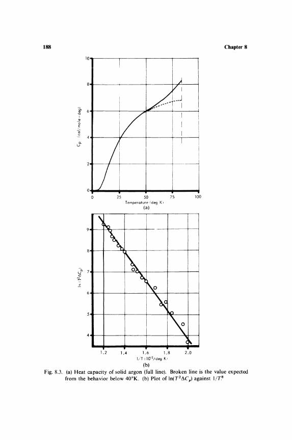
188

"'­u

84-------~----_4------~~--~

0t------P----~------r_----~ o 25

\

8

~

\ 9

50 Temperature I deg K I

(a)

75 100

\ .~

J- 7 <l ~

6

5

4

1.2 1.4

~

~ ~

'" C~ 1.6 1.8 2.0 1/T t 1O-2/deg K,

(b)

Chapter 8

Fig. 8.3. (a) Heat capacity of solid argon (full line). Broken line is the value expected from the behavior below 40oK. (b) Plot of In(T2~C p) against I/T.8

Miscellaneous Problems in Specific Heats 189

the various parameters as the freezing point is approached, the phenomenon of aftermelting in liquids. 10 They may arise from actual melting, at temperatures slightly different from the nominal 1M, in the regions of singularities such as dislocations and grain boundaries, where impurities have segregated. Then the latent heat associated with such regions may be measured as a pseudo specific heat. The subject appears to be somewhat controversial, because some authors 12 have carefully looked for these anomalies but did not find any. All the same, the magnitude and range of the excess specific heat in Fig. 8.3a rule out premelting as the cause of the observed behavior; there is now growing evidence that the explanation is to be sought in the thermal excitation of defects in the solid state.

Studies of diffusion, optical properties, and other phenomena in solids indicate that at temperatures above T;::::: e, the perfect lattice arrangement is disturbed by various kinds of defects. 13 For example, an atom may have moved away from its lattice position, leaving a hole at its site, a vacancy defect, and an atom may occupy a nonlattice vacant space amid other atoms which are at their lattice positions, an interstitial atom. In a simple way, if Ed is the energy needed to form a defect, the number of defects nd at any temperature Twill be given by a Boltzmann factor

nd = no exp (- :i) and the specific-heat contribution from such defects will be

d nod (Ed \ LlCv = dT(nh ) = kT2 exp - kT; (8.8)

Thus, a plot of In(T2LlCJ against liT should be a straight line with a slope - Edlk. Similarly, a plot of In(T2 LlCp ) against liT will be a straight line with a slope - hdlk, where hd is the enthalpy of formation of a defect. Figure 8.3b shows such a plot; the observations do fit the theoretical linear relationship with hd ~ 1250 cal/mole in solid argon. The value is uncertain to about ± 5 %, because LlC p depends slightly upon the method used to extrapolate the specific heat from below about 400K in Fig. 8.3a. Similar LlCp = AT- 2 exp (- BIT) variations have been observed in solid 3He and other substances.

Since the atomic forces and crystal structure of solidified inert gases are well known, several attempts have been made to calculate the values of hd from theoretical models; the values come out to be about 30 % higher than the experimental results. The discrepancy arises from the fact that in the earlier models no relaxation of the stress field was assumed. On the other hand, it is more plausible that the atoms surrounding a vacancy defect move in slightly to

190 Chapter 8

reduce the void, so that the volume of the vacancy is less than that of the atom which left that site. When this is taken into account,t4 there is better agreement \vith the experiments.

Similar specific-heat effects resulting from the presence of defects in the lattice structure are produced by heavy mechanical deforma­tion,15 neutron irradiation, 16 and self-irradiation in radioactive materials. In some cases, the specific heat is reduced, for example, by defects acting as traps for charge carriers in semiconductors and thereby reducing the number of "free" electrons or holes.

8.5. SURF ACE EFFECTS

In the simple discussion of specific heats so far, it has been generally assumed that the internal energy, and hence the specific heat, is proportional to the mass of the substance; that is, they are extensive quantities (Section 1.2). As a matter of fact, statistical mechanics shows that this is a very good approximation (Section 2.5). Nevertheless, in special circumstances, as with finely divided powders, a contribution proportional to the surface area must be considered. It is qualitatively easy to visualize the nature of the effects, taking for simplicity the Debye model for an enumeration of the frequency distribution. In a finite solid, besides the longitudinal and transverse waves which propagate through the solid as if in an infinite medium, there are surface waves of the type considered by Rayleigh, Love, and others. The enumeration of the number of frequencies in a three­dimensional volume V, as in Section 2.5, gives the number of fre­quencies below v as being proportional to Vv\ while it is evident that a similar calculation for a two-dimensional surface of area S will give a term proportional to Sv 2 . Thus, the addition of surface contributions to the Debye term will result in

g(v) dv = 1X1 Vv 2 dv + 1X2SV dv

The corresponding low-temperature specific heat will be

(8.9)

This behavior is indeed found in the specific heat of powdered materials. Figure 8.4 shows the specific heat, in the liquid-helium range, of MgO powder with an area of about 160 M 2/g, which corres­ponds to an edge length of about 100 A if all the particles are in the form of cubes. 1 7 The specific heat is represented well by an equation C = 0.OO459T3 + 0.163T2 mJ/mole·deg, in which the T 3 -term is the usual Debye term.

Miscellaneous Problems in Specific Heats 191

0.12

Vo ~

0

)

cI V

/ Ijl'

0.10

vi ."

~ 0.08 g

~ E

.... ~

0.06

0.04 o 0.1 0.2 0.3 0.4 0.5 0.6 0.7 0.8

1/T (per deg K)

Fig. 8.4. Heat capacity of powdered magnesium oxide with grains of about 100 A size. l ?

The full calculation of the surface contribution is a complex problem which as yet has not been solved satisfactorily. In the continuum model, it is possible to calculate with some difficulty the surface and volume modes of plates and rectangular parallelopipeds. 18

Apart from the usual shortcomings of a continuum model, there is a further assumption that the elastic behavior is not affected by the size of the specimen. On the other hand, it is obvious that the atoms near the surfaces are acted upon by forces very different from those exerted upon the atoms in the interior. Therefore, there is a spatial inhomogeneity of the lattice. The calculations with models of finite lattices are so involved that only beginnings have been made. 19

They show that, apart from the low-temperature effect given by equation (8.9), there should be very small differences at higher tem­peratures, because of the change in optical frequencies resulting from the presence of surface boundaries. The experimental observations are scanty, but it appears that the ST 2-term in equation (8.9) is two to three times larger than the theoretical estimates. 18 A full com­parison between theory and experiment is not easy, because under the experimental conditions, in addition to the total surface area, the shape of the individual particles may also have some influence. Further, the possibility of thermal motions of whole grains of the

192 Chapter 8

substance, behaving as though they were giant macromolecules, cannot be eliminated. The experiments also suffer from the fact that attaining thermal equilibrium in a fine powder is difficult. There is a real need for further experimental and theoretical studies.

8.6. COMPILATIONS OF SPECIFIC-HEAT DATA

A knowledge of specific heat is useful in so many fields of study that the literature on heat capacities is very extensive and is reported in diverse publications. Without the abstracting services of Chemical Abstracts and Physics Abstracts, the task of searching for the data on any particular material would be inordinately laborious. Apart from these sources, perhaps the best single reference, if the heat capacity of any substance is needed, is the sixth edition of Lando/t­Bornstein Zahlenwerte and Funktionen, Vol. 2, Part 4 (Springer­Verlag, Berlin, 1961, 863 pages). This gives an exhaustive listing of the heat capacities of almost all materials investigated before 1958-1959. Special data of cryogenic interest are collected in the various publications of the National Bureau of Standards Cryogenic Engineer­ing Laboratory, Boulder, Colorado. For example, A Compendium of the Properties of Materials at Low Temperatures (V. J. Johnson, editor, 1957) and Specific Heats and Enthalpies of Technical Solids at Low Temperatures (by R. J. Corruccini and J. J. Gniewek, 1960) contain useful information about the specific heat and other properties below 3000 K. There are, of course, other reports by several groups of workers on various aspects of specific-heat studies, such as Debye temperatures or the properties of metals and gases; the references to them may be found without difficulty from the recent reviews cited at the end of the earlier chapters.

In the construction of calorimeters and other pieces of cryogenic equipment, various low-melting solders, glues, varnishes, and technical solids are often used. Their specific heats are needed for the design of such apparatus, especially because weight-for-weight they may contribute more thermal capacity than the standard construction materials such as copper, brass, and stainless steel. Unfortunately, the heat capacity depends upon the purity, method of preparation, and composition of these substances, so that for accurate work each sample must be individually investigated. For many other purposes, it is convenient to have some approximate values. Even so, no handy tabulation of the many measurements is available, and hence Table 8.1 is given here as a summary of the properties of several such auxiliary materials used in cryogenic equipment.

The specific heats of several materials are quite high compared to those of, say, copper. In particular, if the heat capacity of some

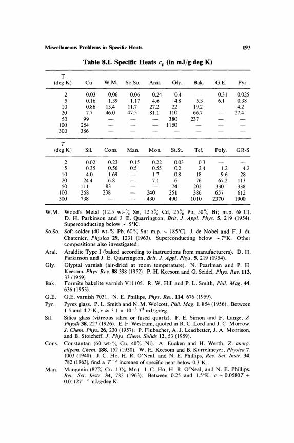
Miscellaneous Problems in Specific Heats 193

Table 8.1. Specific Heats cp (in mJjg·deg K)

T (degK) Cu W.M. So.So. Aral. Gly. Bak. G.E. Pyr.

2 0.03 0.06 0.06 0.24 0.4 0.31 0.025 5 0.16 1.39 1.17 4.6 4.8 5.3 6.1 0.38

10 0.86 13.4 11.7 27.2 22 19.2 4.2 20 7.7 46.0 47.5 81.1 110 66.7 27.4 50 99 380 237

100 254 1150 300 386

T (deg K) Sil. Cons. Man. Mon. St.St. Tef. Poly. GR-S

2 0.02 0.23 0.15 0.22 0.03 0.3 5 0.35 0.56 0.5 0.55 0.2 2.4 1.2 4.2

10 4.0 1.69 1.7 0.8 18 9.6 28 20 24.4 6.8 7.1 6 76 67.2 113 50 111 83 74 202 330 338

100 268 238 240 251 386 657 612 300 738 430 490 1010 2370 1900

W.M. Wood's Metal (12.5 wt-% Sn, 12.5% Cd, 25% Pb, 50% Bi; m.p. 68°C). D. H. Parkinson and J. E. Quarrington, Brit. J. Appl. Phys. 5, 219 (1954). Superconducting below ~ 5°K.

So. So. Soft solder (40 wt- % Pb, 60 % Sn; m.p. ~ 185°C). J. de Nobel and F. J. du Chatenier, Physica 29, 1231 (1963). Superconducting below ~7°K. Other compositions also investigated.

Aral. Araldite Type I (baked according to instructions from manufacturers). D. H. Parkinson and J. E. Quarrington, Brit. J. Appl. Phys. 5, 219 (1954).

Gly. Glyptal varnish (air-dried at room temperature). N. Pearlman and P. H. Keesom, Phys. Rev. 88 398 (1952). P. H. Keesom and G. Seidel, Phys. Rev. 113, 33 (1959).

Bak. Formite bakelite varnish V11105. R. W. Hill and P. L. Smith, Phil. Mag. 44, 636 (1953).

G.E. G.E. varnish 7031. N. E. Phillips, Phys. Rev. 114,676 (1959). Pyr. Pyrex glass. P. L. Smith and N. M. Wolcott, Phil. Mag. 1,854 (1956). Between

1.5 and 4.2°K, c "" 3.1 X 10- 3 T3 mJ/g·deg. Sil. Silica glass (vitreous silica or fused quartz). F. E. Simon and F. Lange, Z.

Physik 38,227 (1926). E. F. Westrum, quoted in R. C. Lord and J. C. Morrow, J. Chern. Phys. 26, 230 (1957). P. Flubacher, A. J. Leadbetter, J. A. Morrison, and B. Stoicheff, J. Phys. Chern. Solids 12, 53 (1959).

Cons. Constantan (60 wt-% Cu, 40% Ni). A. Eucken and H. Werth, Z. anorg. a/lgern. Chern. 188, 152 (1930). W. H. Keesom and B. Kurrelmeyer, Physica 7, 1003 (1940). J. C. Ho, H. R. O'Neal, and N. E. Phillips, Rev. Sci. Instr. 34, 782 (1963), find a T- 2 increase of specific heat below 0.3°K.

Man. Manganin (87% Cu, 13% Mn). J. C. Ho, H. R. O'Neal, and N. E. Phillips, Rev. Sci. Instr. 34, 782 (1963). Between 0.25 and 1.5°K, c ~ 0.0580T + O.0112Y- 2 mJ/g·deg K.

194 Chapter 8

Mon. Monel (67 wt-% Ni, 30% Cu, 1.5% Fe, 1% Mn). W. F. Hampton and 1. H. ~1ennie, Can. J. l?es. 7, 677 (1932). W. H Keesom and B. Kurrelmeyer. Physica 7, 1003 (1940).

St.St. Stainless steel. R. Kohlhass and M. Braun, Arch. Eisenhutlenw. 34, 391 (1963). F. 1. du Chatenier, B. M. Boerstoel, and 1. de Nobel, Physica 31, 1061 (1965). Below ~ 300oK, values are nearly the same for i'-iron, manganese steel, and chrome-nickel steel.

Tef. Teflon (polytetrafluoroethylene). Material has a transition around 160oK. G. T. Furukawa, R. E. McCoskey, and G. 1. King, J. Res. Nat. Bur. Std. 49,273 (1952). Between 1.4 and 4.2°K, R. 1. Noer, C. W. Dempsey, and 1. E. Gordon, Bull. Am. Phys. Soc. 4, 108 (1959), give c ~ 40 X 1O- 3 r 3 ml/g'deg for teflon, c - 63 x 10- 3r3 for polystyrene, and c - 35 x 10- jr' for lucite. W. Reese and 1. E. Tucker, J. Chern. Phys. 43, 105 (1965), give values for tetlon, nylon, and Kel-F (1 to 4 OK) also.

Poly. Amorphous polyethylene. Glassy transition 200oK. B. Wunderlich, J. Chern. Phys. 37, 1203 (1962). (Material with various degrees of crystallinity also investigated.) I. V. Sochava and O. N. Trepeznikova, Soviet Phys. Doklady 2, 164 (1957). (Data for polyvinyl alcohol also given.)

GR-S. GR-S (Buna S) rubber (I,3-butadiene with 25 wt-~';; styrene). Second-order transition with hysteresis around 2100 K. R. D. Rands, W. F. Ferguson, and 1. L. Prather, J. Res. Nat. Bur. Std. 33, 63 (1944). Natural rubber studied by N. Bekkedahl and H. Matheson, J. Res. Nat. Bur. Std. 15, 505 (1934).

substance with low specific heat is to be measured, the thermal capacity of a small amount of glue or solder used for attaching the heater or thermometer may be comparable to that of the specimen under study. Further, constantan and manganin, widely used for winding heaters, are quite unsuitable below about 0.5°K because of the T- 2 increase. At O.l°K, for example, the specific heat of manganin is nearly 103 times that of copper.

8.7. TABULATIONS OF SPECIFIC-HEAT FUNCTIONS

The Einstein and Oebye functions are widely used in calculating the thermodynamic properties of gases and solids, as discussed in detail elsewhere in this monograph. The Oebye function for the internal energy is also useful in cryogenic practice for calculating the amount of refrigeration needed to cool an apparatus. For example, let us calculate the amount of liquid 4He spent if its latent heat, equal to 0.62 callcc, is used to cool 1 gram-atom of copper (1 gram-atom = 63.6 g of copper, Oebye temperature of copper ~ 3100 K) from 300, 90, or 200K to 4.2°K. Strictly, it is the change in enthalpy t1H = SCpdT of copper which must be used for this purpose rather than an estimate of the change in the internal energy t1E = SCv dT. However, Cp - Cv ,

which depends upon the expansion coefficient and compressibility and hence is not easily tabulated as a function of T 10, is usually small enough to permit the calculation to be done using t1E without any serious error. Further, copper has no specific-heat anomaly in this

Miscellaneo~ Problems in Specific Heats 195

Table S.I1

e E(Debye) E(Debye) T T 3RT cal/mole

300 1.03 0.666 1200 90 3.44 0.233 126 20 15.5 0.005 0.6 4.2 74 0.00004 0.001

region. So for various values of 81T, we look up the values of the Debye energy function E(Debye)/3R T in the Appendix and write out a table (Table 8.11), taking for simplicity R ~ 2 caljmole·deg.

The change in internal energy between room temperature and liquid-helium temperature is about 1200 caljmole. If the latent heat of liquid helium is used to bring about this reduction of temperature, about 2000 cc will be spent. A similar calculation shows that 200 cc is needed to cool 63.6 g of copper from 90 to 4.2°K, and only 1 cc from 20 to 4.2°K. The tremendous advantage of precooling any apparatus with liquid air and liquid hydrogen in order to conserve the supply of liquid helium was mentioned even in the Introduction.

Many tabulations of the Einstein and Debye functions were mentioned in Chapter 2. Some of these tables, especially the older ones, should be used with caution since the value of R different from the present accepted 8.314 J Imole·deg = 1.987 caljmole·deg has been used in them. The error caused by this is serious only at high tem­peratures, where the Debye specific heat approaches its limiting value of 3R. A 1 % error in the specific heat at T - 8 gives an error of nearly 10 % in the calculated value of 8. One way to make the tables permanently useful is to give the values in a dimensionless form, that is, give Cv!3R rather than Cv . Then, to find the specific heat at any given T18, the entries must be multiplied by 3R, but the tables themselves need not be changed every time an improvement in our knowledge of the value of R takes place. This is the procedure followed in the tabulations of Overton and Hancock for the Einstein functions and those of Beattie for the Debye functions, which are at present the most accurate ones available. For rough calculations, a table to three figures is often sufficient, but for a variety of refined calculations it is necessary to have more accurate tables. Un­fortunately, six-figure tables are not easily accessible. Beattie's six­figure tables were published in 1926, though they have been recently checked for accuracy, while the eight-figure tables of Overton and Hancock and the detailed tables of Hilsenrath and Ziegler are contained in laboratory reports rather than professional journals.

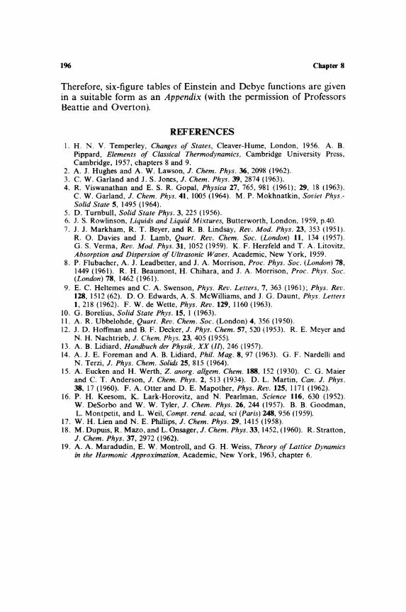
196 Chapter 8

Therefore, six-figure tables of Einstein and Debye functions are given in a suitable form as an Appendix (with the permission of Professors Beattie and Overton).

REFERENCES

I. H. N. V. Temperley, Changes of States, Cleaver-Hume, London, 1956. A. B. Pippard, Elements of Classical Thermodynamics, Cambridge University Press, Cambridge, 1957, chapters 8 and 9.

2. A. l. Hughes and A. W. Lawson, J. Chem. Phys. 36, 2098 (1962). 3. C. W. Garland and l. S. lones, J. Chem. Phys. 39, 2874 (1963). 4. R. Viswanathan and E. S. R. Gopal, Physica 27, 765, 981 (1961); 29, 18 (1963).

C. W. Garland, J. Chem. Phys. 41, 1005 (1964). M. P. Mokhnatkin, Soviet Phys.­Solid State 5, 1495 (1964).

5. D. Turnbull, Solid State Phys. 3, 225 (1956). 6. 1. S. Rowlinson, Liquids and Liquid Mixtures, Butterworth, London, 1959, p.40. 7. J. J. Markham, R. T. Beyer, and R. B. Lindsay, Rev. Mod. Phys. 23, 353 (1951).

R. O. Davies and J. Lamb, Quart. Rev. Chern. Soc. (London) 11, 134 (1957). G. S. Verma, Rev. Mod. Phys. 31, 1052 (1959). K. F. Herzfeld and T. A. Litovitz, Absorption and Dispersion of Ultrasonic Waves, Academic, New York, 1959.

8. P. Flubacher, A. J. Leadbetter, and l. A. Morrison, Proc. Phys. Soc. (London) 78, 1449 (1961). R. H. Beaumont, H. Chihara, and J. A. Morrison, Proc. Phys. Soc. (London) 78, 1462 (1961).

9. E. C. Heltemes and C. A. Swenson, Phys. Rev. Letters, 7, 363 (1961); Phys. Rev. 128, 1512 (62). D. O. Edwards, A. S. McWilliams, and J. G. Daunt, Phys. Letters 1,218 (1962). F. W. de Wette, Phys. Rev. 129, 1160 (1963).

10. G. Borelius, Solid State Phys. 15, I (1963). II. A. R. Ubbelohde, Quart. Rev. Chem. Soc. (London) 4,356 (1950). 12. J. D. Hoffman and B. F. Decker, J. Phys. Chem. 57,520 (1953). R. E. Meyer and

N. H. Nachtrieb, J. Chern. Phys. 23, 405 (1955). 13. A. B. Lidiard, Handbuch der Physik, XX (II), 246 (1957). 14. A. J. E. Foreman and A. B. Lidiard, Phil. Mag. 8,97 (1963). G. F. Nardelli and

N. Terzi, J. Phys. Chern. Solids 25,815 (1964). 15. A. Eucken and H. Werth, Z. anorg. aI/gem. Chem. 188, 152 (1930). C. G. Maier

and C. T. Anderson, J. Chern. Phys. 2, 513 (1934). D. L. Martin, Can. J. Phys. 38,17 (1960). F. A. Otter and D. E. Mapother, Phys. Rev. 125, 1171 (1962).

16. P. H. Keesom, K. Lark-Horovitz, and N. Pearlman, Science 116, 630 (1952). W. DeSorbo and W. W. Tyler, J. Chem. Phys. 26, 244 (1957). B. B. Goodman, L. Montpetit, and L. Weil, Compt. rend. acad, ~ci (Paris) 248, 956 (1959).

17. W. H. Lien and N. E. Phillips, J. Chem. Phys. 29,1415 (1958). 18. M. Dupuis, R. Mazo, and L. Onsager, J. Chem. Phys. 33, 1452, (1960). R. Stratton,

J. Chem. Phys. 37, 2972 (1962). 19. A. A. Maradudin, E. W. Montroll, and G. H. Weiss, Theory of Lattice Dynamics

in the Harmonic Approximation, Academic, New York, 1963, chapter 6.

Appendix

The six-figure tables give the values of the internal energy E and heat capacity at constant volume Cv of solids in the Einstein and Oebye models. The functions are tabulated in a dimensionless form as follows to make them permanently useful:

A. Einstein internal energy function [equation (2.9a)]:

E (Einstein) x hVE TE 3RT eX - 1

x=-=-kT T

B. Einstein specific-heat function [equation 2.7)]:

C v (Einstein) x 2 ex

3R (eX - 1)2

C. Oebye internal energy function [equation (2.16a)]:

E (Oebye) = ~[ x3 dx 3RT x 3 eX - 1 o

O. Oebye specific-heat function [equation (2.17)]:

£) X=-

T

The presently accepted value of R is 1.987 caljmole' deg, or 8.314 J/mole·degK.

The functions A to 0 are tabulated at intervals of 0.01 over the useful range, namely, TE/T < 16 in the Einstein functions and efT < 24 in the Oebye functions. Over most of the range, a linear interpolation gives an accuracy of nearly three to four units in the sixth significant figure. However, interpolation with second differences is recommended for accurate work. Following the usual procedure, a reduction by one unit of the fixed "characteristic" part is indicated by an underscoring

197

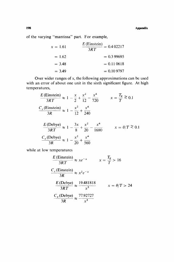
198

of the varying "mantissa" part. For example,

x = 1.61

= 1.62

= 3.48

= 3.49

= 0.399695

= 0.11 0618

= 0.109797

Appendix

Over wider ranges of x, the following approximations can be used with an error of about one unit in the sixth significant figure. At high temperatures,

E (Einstein) x x2 X4

3RT ~ 1 - 2" + 12 - 720 TE '"

X = T < 0.1

C v (Einstein) x2 X4

3R ~ 1 - 12 + 240

E (Debye) 3x x2 X4

3RT ~ 1 - 8 + 20 - 1680 x = elT <: 0.1

C v (De bye ) x 2 X4

3R ~ 1 - 20 + 560

while at low temperatures

E (Einstein) _ ----;:;::;xe x

3RT TE

X = T > 16

C v (Einstein) 2---'----- ~ x e x

3R

E (Debye) 19.481818 ---- ~ ------c~-

3RT x3 x = elT > 24

C v (Debye) 77.92727 3R ~ x3

A. Einstein Internal Energy Function E (Einstein}/3R T

E(Einstein)/3 RT

x

0.0

0.1 0.2 0.3

0.4 0.5 0.6

0.1 0.8 0.9

1.0

1.1 1.2 1.3

1.4 1.5 1.6

1.1 1.8 1.9

2.0

2.1 2.2 2.3

2.4 2.5 2.6

3.0

3.1 3.2 3.3

3.4 3.5 3.6

3.1 3.8 3.9

o 1 2 3 4 5 6 1 8 9

1.0 00000 95008 2QQll .!!2.Q12 80133 15208 10300 65408 ~ ~

.9 50833 46008 41200 36408 31633 26814 22132 11401 12699 08001 9 03331 ~ ~ ~ ~ 8020~ ~ 71068 ~ ~ 8 51489 52996 48519 44059 396I5 3518 30111 26382 22004 I7b43

.8 13298 08969 04651 00361 96082 91818 ~ ~ ~ ~ 1 10141 66582 62432 58299 54183 50082 45998 41930 31811 33841 1 29822 25818 21830 11858 13903 09963 06039 02131 98240 94364

.6 90504 86660 82831 19019 15222 11441 61616 63921 60193 56415 6 52113 49086 45415 41160 38120 34496 30881 21293 23115 20153 6 16606 13014 09558 06051 02511 22lQ! ~ 92206 88181 §2lIl

0.581911 18591 15233 11884 68549 65230 61926 58636 55361 52102

5 48851 45621 42411 39211 36025 32853 29691 26554 23421 20314 5 11215 14131 11062 08006 04965 01939 ~ ~ ~ ~ 4 81020 84018 81151 18238 15339 12453 69582 66124 63881 61051

.4 58235 55433 52644 49810 41108 44361 41621 38906 36199 33506 4 30825 28159 25505 22865 20238 11624 15024 12436 09862 01301 4 04153 02211 ~.21!.!!§. ~ ~.llill ~ 84831 82398

.3 19978 77570 75175 72792 70422 68064 65719 63386 61065 58757 3 56461 54176 51904 49645 41391 45161 42931 40725 38525 36337 3 34160 31996 29843 27701 25572 23453 21347 19252 17168 15096

0.3 13035 10986 08948 06921 04905 02900 00907 ~ ~ ~

.2 93044 91105 89178 87261 85355 83459 81515 19101 77838 75985 2 74143 72311 70490 68679 66879 65088 63308 61539 59119 58030 2 56291 54562 52842 51133 49434 47745 46065 44396 42736 41086

.2 39445 37814 36193 34581 32979 31386 29803 28229 26665 25110 2 23564 22027 20500 18981 17472 15972 14480 12998 11525 10061 2 08605 07158 05721 04291 02871 01459 00056 98661 ~ ~

.1 94528 93161 91815 90471 89135 87808 86488 85177 83874 82519 1 81293 80014 78743 77480 16225 74978 13738 12507 11283 10061 1 68858 61658 66464 65219 64101 62930 61161 60611 59462 58321

0.15 1187 6060 4941 3829 2124 1626 0535 ~ mA. :wM

.14 6241 5184 4135 3092 2051 1028 0005 ~ 1W ~ 13 5982 4993 4010 3033 2063 1099 0142 .2lli. 8246 ~ 12 6316 5449 4530 3616 2708 1806 0910 0021 illl !!!.22.

.11 7387 6520 5660 4805 3951 3113 2216 1444 0618 mb 10 8982 8112 1368 6569 5116 4988 4206 3429 2651 10 1129 0312 ~ ~ 81348 1l22l 66685 ~ 2m ~

.09 31960 30902 23893 16933 10020 03156 ~ ~ 82841 16111 08 69542 62959 56421 49930 43484 31083 30121 24415 18141 11924 08 05144 ~ llID. ~ 81458 1.2ill. illl.Q. ~ ~ 2!.Q2l

201

202 E(Emein)/3 RT

o 2 4 5 6 8 9

4.0 0.07 46294 40578 34903 2926B 23673 1811( 12602 07126 olGBB L612Q

4.1 4.2 4.3

4.4 4.5 4.6

4.7 4.8 4.9

5.0

5·1 5.2 5.3

5.4 5.5 5.6

5.7 5.8 5.9

.06 ~0930 85609 80326 75080 69872 64702 59569 54472 49413 44389 06 39402 34451 29536 24656 19812 15002 10228 05488 00782 96111 O~ 91473 86870 82299 77763 73259 68788 64349 59943 55569 512?8

.05 46918 42639 38392 34176 29991 25837 21714 17620 13557 09524 05 05521 01547 21.§.9.£ lli.§l 89801 §22.U 82114 illlllllli ~ 04 67079 63390 59729 56094 52487 48907 45353 41826 38325 34850

.04 31402 27979 24582 21210 17863 14542 11246 07974 04727 01504 03 98306 95132 91981 88855 85752 82672 79616 76583 73572 70585 03 67620 64678 61758 58860 55984 53130 50298 47487 44698 41930

0.03 39183 36457 33752 31067 28403 25759 23136 20532 17949 15385

.03 12841 10317 07812 05326 02859 00412 ~ ~ 2ll§l 90808 02 88453 86116 83797 81496 79213 76948 74700 72470 70257 68061 02 65882 63720 61574 59446 57334 55238 53159 51095 49048 47017

.02 45002 43002 41018 39050 37097 35159 33236 31329 29436 27558 02 25695 23846 22012 20192 18387 16596 14819 13056 11306 09571 02 07849 06141 04446 02764 01096 ~ ~ 2§llQ 2A22! ~

.01 91360 89782 88217 86664 85123 83594 82078 80573 79081 77600 01 76131 74674 73229 71795 70372 68961 67561 66172 64794 63427 01 62071 60726 59392 58068 56755 55453 54160 52879 51607 50346

6.0 0.014 9095 7854 6622 5401 4190 2988 1796 0613 ~ ~

6.1 6.2 6.3

6.4 6.5 6.6

.013 7122 5977 4842 3715 2598 1490 0390 .21QQ 8218 ~ 012 6081 5025 3978 2939 1909 0887 9873 8868 7870 8 1

011 5900 4927 3962 3004 2054 1113 0118 9252 §.J.E 1421

.010 6517 5620 4730 3848 2973 2105 1244 0390 22ill.!U.Q.ll 009 78707 70445 62250 54123 46062 38067 30138 22274 14474 06138 008 99066 91457 83910 76425 69002 61640 54338 47096 39914 32792

6.7 .008 25727 18721 11773 04882 98048 ~ 8454877882 1!£1l 64114 6.8 007 58212 51763 45367 39025 3273526497 20311 14175 08091 02057 6.9 006 96073 90139 84254 78418 72630 66891 61199 55554 49956 44405

7.0 0.006 38900 33441 28027 22658 11334 12054 06818 01626 ~ ~

7.1 7.2 7.3

7.4 7.5 7.6

7.7 7.8 7.9

.005 86308 81287 76308 71370 66474 61619 56804 52029 47294 42599 005 37943 33327 28748 24208 19707 15242 10816 06426 02073 2l12l 004 93477 89232 85024 80851 76712 72609 68540 64505 60505 56537

.004 52604 48703 44835 41000 37197 33426 29687 25979 22303 18657 004 15043 11459 07905 04381 00887 ~ ~ ~ 87203 83~54 003 80534 77241 73976 70739 67530 64347 61192 58063 54961 51 85

.003 48835 45811 42813 39840 36892 33969 31071 28198 25349 22525 003 19724 16948 14194 11465 08758 06075 03414 00776 98160 ~62 002 92996 90447 87919 85413 82929 80465 78023 75601 73201 ~

E(Eimitein)/3 RT

x o 2 3 4 5 6 7 8 9

8.0 0.002 68460 66120 63800 61500 59220 56959 54717 52495 50292 48107

8.1 .002 45941 43794 41665 39555 37462 35387 33330 31291 29269 27265 8.2 002 25278 23308 21354 19418 17498 15595 13708 11837 09982 08143 8.3 002 06320 04513 02721 00945 ~ ~ ~ 2l22l 92290 2Q£Q1

8.4 .001 88931 87273 85630 84001 82386 80785 79197 77623 76063 74517 8.5 001 72983 71463 69956 68462 66981 65513 64058 62615 61184 59766 8.6 001 58360 56966 55585 54215 52857 51511 50177 48854 47543 46243

8.7 .001 44954 43676 424104115439909 38676 37452 36240 35038 33846 8.8 001 32665 31494 30333 29183 28042 26911 25790 24688 23577 22485 8.9 001 21403 20330 19266 18211 17166 16130 15103 14084 13075 12074

9.0 0.0011 1083 0099 2ill 8158 ll.Q!. 6251 2llQ ~ Jill ~

9.1 .00101627 0726 ~ ~ 80711 72014 ~ ~ illll ill§Q 9.2 0009 29656 21406 13227 05120 ~ 89118 BI222 lll22 ~ ~ 9.3 0008 50323 42767 35277 27852 20492 13197 05966 ~ ~ ~

9.4 .0007 77671 70751 63892 57094 50355 43675 37054 30491 23985 17537 9.5 0007 11146 04810 ~ lliQ£ 86136 80020 1..12..22. lli2Q §lm ~ 9.6 0006 50240 44440 38b9f 32993 27345 21747 16198 10698 0524b ~

9.7 .0005 94486 89178 83915 78700 73530 68406 63327 58293 53303 48358 9.8 0005 43456 38597 33781 29008 24277 19587 14939 10332 05766 01240 9.9 0004 96754 92308 87901 83533 79204 74913 70659 66444 62266 58125

10.0 0.0004 54020 49952 45919 41923 37962 34036 30144 26287 22465 18676

10.1 .0004 14921 11199 07510 03853 00229 ~ ~ ~ 86053 ~ 10.2 0003 79151 75747 72372 69028 65713 62427 59171 55944 52745 49575 10.3 0003 46433 43318 40232 37173 34141 31136 28158 25206 22281 19381

10.4 .0003 16507 13659 10837 08039 05266 02518 ~ ~ 94420 ~ 10.5 0002 89141 86536 83955 81397 78861 76348 73858 71390 68944 66519 10.6 0002 64116 61735 59375 57036 54717 52420 50143 47886 45650 43433

10.7 .0002 41236 39059 36901 34763 3264430543 28461 263982435422327 10.8 0002 20319 18329 16356 14402 12464 10544 08641 06755 04886 03034 10.9 0002 01198 .2.2.ll2 21.2li 2.2I!\2 ~ 92264 ~ 88801 87092 85400

11.0 0.0001 83722 82059 80411 78778 77160 75556 73966 72391 70830 69283

11.1 11. 2 11. 3

.00016 7749 6230 4724 3231 1752 0287 8834 1122 ~ A25A 00015 3153 1765 0388 2Q£2 7673 £114 2QQ1 l22I 2388 ~ 00013 9816 8547 7290 6044 4809 3585 2373 1171 ~ ~

11.4 .00012 7630 6471 5322 4184 3056 1938 0830 ~ 8644 7566 11.5 00011 6497 5438 4389 3349 2319 1297 0285 9282 8289 llQi 11.6 00010 6328 5360 4402 3452 2511 1578 0653 97374 88296 I2lQQ

11.7 .00009 70385 61550 52796 44120 35523 27003 18560 10194 01903 ~ 11.8 00008 85544 77476 69481 61557 53706 45925 38215 30574 23002 15499 11. 9 00008 08064 00696 lli.2i ~ ~ llil3J. 64842 ~ 22:l.2!. 441QQ

203

204

x

!2.0

12.1 12.2 12.3 12.4 12.5 12.6

12.7 12.8 12.9

13.0

£(Einsteio)j3 RT

o 2 4 5 6 B 9

0.00007 37310 30582 23915 17308 10761 04273 97844 ~1 85160 78904

.00006 72705 66562 60474 54442 48464 42541 36671 30854 25090 19379 00006 13719 08110 02552 ~ 21588 86180 80821 1221l 70248 6202i 00005 59867 54747 49673 44b46 39664 34727 29835 2~f 20184 15424

.00005 10707 06033 01402 96812 ~ ~ ~ 78868 74483 1Q!li 00004 65833 61567 57340 53151 49000 44887 40811 36772 32770 28805 00004 24875 20982 17123 13300 09512 05758 02038 ~ 94700 9108Q

.00003 87494 83941 80419 76930 73473 70047 66652 63288 59955 56653 00003 53380 50137 46924 43740 40585 37458 34361 31291 28249 25236 00003 22249 19290 16358 13453 10574 07721 04894 02094 ~ ~

0.00002 93843 91143 88468 85817 83190 80588 78009 75453 72921 70412

13.1 .00002 67926 65462 63021 60603 58206 55832 53479 51147 48837 46548 L3.2 00002 44280 42032 39806 37599 35413 33246 31100 28973 26865 24777 13.3 00002 22708 20658 18626 16613 14619 12643 10685 08744 06822 04917

13.4 .00002 03C"0 01159 ~ 2liIQ 2.2£2!. 93848 92062, m2 ~ 86801 13.5 00001 85080 83374 81684 80009 78350 76705 75076 73462 71863 70278 13.6 00001 68708 67152 65610 64083 62569 61070 59584 58112 56653 55207

13·7 .00001 53775 52356 50950 49557 48177 46809 45454 44112 42781 41463 13.8 00001 40157 38863 37581 36311 35052 33805 32569 31345 30132 28930 13.9 00001 27739 26558 25389 24231 23083 21946 20819 19702 18596 17500

14.0 0.000011 6414 5338 4272 3216 2169 1132 0105 9087 8078 7078

14.1 .000010 6088 5107 4135 3172 2218 1272 0335 94071 84874 75762 14.2 000009 66734 57789 48926 40145 31444 22824 14283 05820 9743 6 §9~~ 14.3 000008 80897 72742 64662 56656 48724 40865 33079 25364 17720 10146

14.4 .000008 02643 ~ 87842 80544 73313 66148 22Q2Q 52017 ~ 38145 14.5 000007 31304 24527 17812 11159 04568 98037 ~ ~ 78804 lS2lQ 14.6 000006 66275 60097 53977 47912 41904 35951 30053 24209 18420 12683

14.7 .000006 07000 01369 221JQ 22£.6.i 84786 lillQ 7398.4 68658 63381 ~8153 14.8 000005 52973 47840 42755 37717 32726 277S1 22881 18027 13217 08452 14.9 000005 03731 22Q.21 ~ 89828 run ~ 76306 71882 ~ 63156

15.0 0.000004 58854 54591 50367 46183 42037 37930 33861 29829 25834 21877

15.1 .000004 17956 14071 10222 06409 02631 98888 ~ 2!2Q£ 87866 84260 15.2 000003 80687 77147 73639 70165 66722 63311 59932 56584 53268 49981 15.3 000003 46726 43500 40304 37138 34001 30893 27814 24764 21742 18747

1~.4 .000003 15781 12842 09930 07045 04187 01355 ~ 95770 2l2ll ~0289 15.5 000002 87586 84908 52255 79626 77022 74442 71886 69354 66845 64360 15.6 000002 61897 59457 57040 54646 52273 49923 47594 45287 43001 40737

15.7 .000002 38493 36271 34069 31887 29726 27584 25463 23361 21279 19216 15.8 000002 17172 15147 13141 11154 09185 07234 05302 03387 01490 ~ 15.9 000001 97749 95905 94077 92267 90473 88696 86936 85192 83464 81752

16.0 0.000001 80056 E/3RT -

-x xe when x > 16

B. Einstein Specific Heat Function Cv (Einstein)j3R

C .(Einstein)/3 R

0.0

0.1 0.2 0.3

0.4 0·5 0.6

0.7 0.8 0.9

1.0

1.1 1.2 1.3

1.4 1.5 1.6

1.7 1.8 1.9

2.0

2.1 2.2 2.3

2.4 2.5 2.6

2.7 2.8 2.9

3.0

3.1 3.2 3·3

3.4 3.5 3.6

3.7 3.8 3.9

o 2 4 5 6 7 8 9

1.0 00000 ~ 222tl 2.2.2£2 ~ m.2£ 22lQQ. ~ ~ 22.R2

.9 99167 98992 98801 98593 98368 98127 97869 97595 97304 96997 9 96673 96333 95976 95603 95214 948C8 94386 93947 93d92 93021 9 92534 92030 91510 90974 90422 89854 E9270 88669 88053 87421

.9 86773 86109 85429 84733 84022 83295 82552 81793 81019 80230 9 79425 78604 77768 76917 76050 75168 74271 73359 72432 71490 9 70532 69560 68573 67571 66555 65523 64477 63417 62341 61252

.9 60148 59030 57897 56750 55589 5d415 53226 52023 50806 d9~75 9 48331 47073 45801 44516 43218 41906 40581 392d2 37891 36526 9 35148 33758 32354 30938 29509 28068 26614 25147 23668 22177

0.9 20674 19158 17630 16091 14540 12976 11401 09815 08217 06607

.9 04986 03354 01710 00056 ~ 967~g ~ 93328 ~16l9 ~ 8 88170 86430 84679 82918 ~ 793 77575 75774 739b4 72144 8 70314 68474 66626 64768 62900 61024 59139 57244 55341 53429

.8 51509 49580 47642 45696 43742 41780 39809 37831 35844 33850 8 31849 29839 27822 25798 23766 21728 19682 17629 15569 13502 8 11429 09349 07262 05169 03070 00964 ~ ~ 94610 92481

.7 903458820486057 83905 81747 7958477416 75243 7306470881 7 68693 66500 64303 62101 59894 5768d 55469 53249 51026 48799 7 46568 44333 42094 39852 37606 35356 33104 30848 28589 26321

0.7 24062 21794 19523 17249 14973 12694 10413 08130 05844 03556

.7 01266 ~ 96680 94384 92086 89787 87486 ~518g 82880 8057§ 6 78269 7596I 13652 71343 69032 66721 64408 209 59782 57A6 6 55154 52839 50524 48209 45893 43578 41262 38941 36632 34317

.6 32002 29688 27374 25061 22748 20437 18125 15815 13506 11197 6 08890 06584 04219 01975 22§1l illll. ~ m1A ~ ~8183 585890835988130979021 7b736 7445272171 b9892b7bI5 5340

.5 63068 60798 58530 56265 54003 51743 49486 47232 44980 42732 5 40486 38244 36004 33767 31534 29304 27077 24853 22633 20416 5 18203 15993 13786 11584 09385 07189 04997 02810 00625 ~

0.4 96269 94091 91929 89164 87604 85448 83296 81149 79006 76867

.474732 12602 70476 68355 66238 64125 62018 59915 57816 55722 4 53633 51549 49470 47395 45325 43260 41200 39145 37095 35050 4 33010 30975 28946 26921 24901 22887 20878 18814 16876 14882

.4 12894 10912 08935 06963 04996 03036 01080 22llQ ~ ~ 3 93313 91386 89463 87547 85636 83731 81831 19937 78049 76167 3 74290 72419 10554 68695 66841 64993 63152 61316 59486 57661

.3 55843 54031 52224 50424 48629 46840 45058 43281 41510 39746 3 37987 36234 34488 32747 31012 29284 27562 25845 24135 22431 3 20733 19041 17355 15675 14001 12333 10672 09017 07367 05724

208 C .(Einstein) /3 R

x o 2 9

4.0 0.3 04087 02456 lCP32 992U 97601 2.22.2.2 943:4 92eoo 91213 89631

4.1 .2 86055 86486 84923 83365 81814 80270 78731 77198 75672 74152 4.2 72637 71129 69627 68132 66642 65158 63681 62210 60744 59285 4.l :7832 56385 549L4 53509 52081 50658 49241 47831 46426 45027

4.4 .2 43635 42248 40868 39494 38125 36763 35406 34056 32711 31372 4.5 2 3004028713 27392 26077 24768 23465 22168 20877 19591 18312 4.6 2 17038 15770 14508 13?52 12001 10757 09518 08285 07057 05836

4.7 .2 0462003410 02205 01006 ~ 98626 97444 96268 22Q2l 2l2l1 4.8 1 92773 91620 90471 89329 88192 87060 t5934 84814 83699 82589 4.9 1 81485 P0387 79294 78206 77123 76046 74975 73909 72848 71792

5.0 0.17 0742 :!.ti2l ~ 7623 6594 lliQ ill!. llli ~ 1526

5.1 .16 0528 5.2 15 0827 5.3 14 1624

2.2l2. §.ill 7564 £5.1ll. 2§l.1. 4647 3685 2727 1775 9885 lli~ 8015 ~ .§l£5. 5247 4334 3426 .?.2£.l 0731 9842 §12§. 8078 7204 6334 ~ 4608 ill.?

5.4 .13 2901 2055 1213 0376 22Al §1!.2 7.§.2l 7072 ~ 2.ill. 5.5 12 4642 5.6 11 6827

3840 3044 2251 1463 0680 ~ 9126 8355 12§1 6070 5317 4568 3823 3082 2346 i6i3 oR85 0161

5.7 .10 9442 8726 8014 7307 6603 5904 5208 4517 3829 3146 1791 1119 0451 WJ.5. Wl.5. 84713 78189 71704 ~ 52475 46140 39843 33583 27359 21173 15023 08910 02832

5.8 10 246,) 5· 9 09 58847

6.0 0.08 96791 90786 84816 78882 72984 67121 61293 55499 L9741 44017

6.1 .08 38327 32672 27051 21464 15910 1039004904 22i2! 94031 88644 6.2 07 83289 77967 72678 67421 62196 57004 51843 46713 41615 36549 6.3 07 31513 26509 21536 16593 11681 06799 01948 97126 92335 ~l2Il

6.4 .06 82841 78139 73465 68821 64206 59620 55063 50534 46034 41561 6.5 06 37117 32701 28313 23953 19620 15314 11036 0678402560 98363 6.6 05 94192 90048 85930 81838 77772 73733 69719 65731 61768 57831

6.7 .05 53919 50032 46171 42334 38521 34734 30970 27231 23516 19826 6.8 05 16159 12516 08896 05300 01728 98178 94652 91149 87668 84210 6.9 04 80775 77363 73972 70604 67258 63934 60632 57351 54092 50854

7.0 0.04 47638 44443 41269 38116 34984 31873 28782 2571~ 22662 19632

7.1 .04 16623 13633 10663 07714 04783 01873 98982 96110 ~ 90423 7.2 03 87609 84813 82036 79277 76538 73816 71113 68428 65761 63112 7.3 03 60481 57868 55273 52695 50134 47591 45065 42556 4006437590

7.4 .03 35132 32690 30266 27857 25466 23090 20731 18388 16061 13750 7.5 03 11454 09175 06911 04662 02429 00212 98~09 ~22~ ~o ~ 7.6 02 89350 87223 85110 83012.80928 78858 76 03 74762 72736 70723

7.7 .02 68725 66740 64769 62812 60868 58938 57021 55118 53228 51351 7.8 02 49487 47636 45799 43974 42162 40362 38575 36801 35039 33290 7.9 02 31553 29828 28115 2641424725 23049 21384 19730 18089 16459

C.(Einstein)/3 R

o 1 2 3 4 5 6 7 8 9

8.0 0.02 14840 13233 11638 10053 08480 06918 05367 03827 02298 00780

8.1 .01 99273 97776 96291 94815 93350 91896 90452 89018 81595 86182 8.2 01 84779 83385 82002 80629 19266 11912 16568 75234 13909 12594 8.3 01 11288 69992 68105 61421 66159 64900 63649 62408 61116 59952

8.4 .01 58138 51532 56335 55147 53961 52196 51633 50419 49333 48195 8.5 01 41066 45945 44832 43121 42630 41541 40460 39381 38322 31265 8.6 01 36215 35173 34138 33111 32092 31080 30016 29019 28089 21106

8.1 .01 26131 25163 24202 23241 22300 21360 20421 19501 18582 11669 8.8 01 16163 15864 14911 14085 13205 12332 11466 10606 09152 08904 8.9 01 08063 07228 06399 05571 04160 03950 03145 02341 01554 00761

9.0 0.009 99866 92116 84423 76188 69210 61688 54222 46812 39451 32151

9.1 .009 24911 11120 10582 03498 9~4~~ 89488 8g5~1 15681 68864 6209g 9.2 008 55310 48100 42019 35508 2 9 22513 1 0 9 09114 ~ ~ 9.3 001 90813 84681 18541 12454 66401 60406 54449 48538 42611 36849

9.4 .001 31011 25336 19645 13991 08391 02828 2llQl 91828 ~ §222! 9.5 00615639 10324 65050 59815 54621 49466 4435039213 3423529235 9.6 006 24213 19348 14462 09612 04800 00024 ~ 90582 ~ 81283

9.1 .005 16681 12126 61600 63108 58651 54228 49839 45484 41161 36812 9.8 005 32616 28393 24202 20043 15916 11820 01151 03124 ~ 2215g 9.9 004 91811 81901 84022 80112 16351 12561 68199 65066 6I3b3 51687

10.0 0.004 54041 50422 46831 43268 39133 36225 32144 29290 25862 22461

10.1 .004 19081 15139 12416 09120 05849 02603 ~ ~ ~ 89810 10.2 003 86149 83651 80518 11529 14503 11501 68522 65561 62634 59125 10.3 003 56838 53913 51131 48311 45513 42131 39982 31249 34538 31841

10.4 .003 29118 26529 23901 21294 18101 16141 13594 11068 08561 06014 10.5 003 03606 01158 W£2. IDli ~ ~ 89202 86866 84549 82251 10.6 002 19910 11108 15463 13236 11026 68834 66659 64501 62360 60236

10.1 .002 58129 56038 53964 51906 49865 41839 45830 43836 41858 39896 10.8 002 31950 36018 34102 32201 30316 28445 26589 24141 22921 21108 10.9 002 19310 11521 15151 14002 12260 10532 08818 01118 05431 03158

11.0 0.002 02091 00450 98816 21ill ~ .2.l22£ 92410 90840 89282 !l11.ll.

11.1 .001 86205 84684 83116 81619 80195 18122 11261 15812 14315 12949 11.2 001 11534 10130 68138 61351 65981 64628 63280 61942 60615 59299 11.3 001 51994 56699 55414 54139 52815 51621 50311 49143 41919 46104

11.4 .0014 5500 4305 3119 1944 0111 a620 8413 1334 6205 5084 11.5 0013 3913 2811 1111 0693 ~ ~ lill ~441 2l2.2. ~ 11.6 0012 3341 2324 1316 0316 2ltl ~ 00 lli2 ~ 4481

11.1 .0011 3536 2598 1669 0146 ~ .§lli 8024 1!l!. 6245 ~ 11.8 0010 4495 3631 2113 1923 1019 0243 ~ 85898 11lll ~ 11.9 0009 61602 53635 45132 31893 30118 22401 14151 01110 ~ 92181

209

210 C.(Einstein)/3 R

c 2 5 6 7 8 9

12.0 0.0008 84777 77434 7015! 62927 55761 486;4 41605 34613 27678 20800

12.1 .0008 13977 07211 00499 2)842 ~240 80691 74196 67754 61364 ~ 12.2 0007 48141 42506 36323 30190 24101 18014 12090 06155 00268 94430 12.3 0006 88640 82891 71201 71551 65948 60391 54879 49412 43990 38613

12.4 .0006 33279 27990 22744 11540 12380 01262 02185 9~~ ~ §I£Q2 14.5 0005 82294 77423 72592 67800 63048 58335 53661 49025 44421 39861 12.6 0005 35345 30860 26411 22000 17624 13285 08982 04713 00481 96282

12.1 .000492119 81990 83895 79834 15806 11811 6185063921 60024 56160 12.8 0004 52327 48527 44151 41019 31312 33635 29989 26313 22786 19230 12.9 0004 15103 12205 08136 05295 01883 98500 ~ 91816 88516 85243

13.0 0.0003 81997 18779 75586 72421 69281 66168 63080 60018 56981 53970

13.1 .0003 50983 48022 45085 42112 39284 36419 33519 30761 27968 25197 13.2 0003 22450 19725 17023 14344 11687 09052 06439 03847 01278 ~ 13.3 0002 96202 93696 91211 88746 86302 83879 81475 79092 76728 74384 13.4 .0002 72060 69755 67470 65203 62955 60726 58516 56324 54151 51995 13.5 0002 49858 47738 45637 43552 41486 39436 37404 35388 33390 31408 13.6 0002 29443 2749425561 2364521745·1986017992 16139 14301 12479

13.7 .0002 10672 08881 0710405342 03596 01863 00145 98442 ~ ~ 13.8 0001 93417 91770 90137 88518 86912 85320 83741 82175 80623 79083 13.9 0001 7755776043 74542 73054 71578 70114 68663 61224 65198 64383

14.0 0.00016 2980 1589 0209 88~ li§2 6141 4807 ~ 2174 0874

14.1 .00014 9585 8306 7039 5782 4536 3300 2075 0860 ill2 8461 14.2 00013 7276 6102 4937 3783 2638 1502 0377 9261 8154 7056 14.3 00012 5968 4889 3820 2759 1707 0664 lliQ 8605 ~ 6580

14.4 .00011 5581 4590 3607 2633 1666 0708 2I22. 8~17 ~ ~ 14·5 00010 6039 5129 4226 3332 2444 1564 0692 ~lli2§.~ 14.6 00009 72762 64403 56114 47896 39748 31669 23658 15715 07840 00032

14.7 .00008 92290 84614 71003 69457 61915 54556 47201 39908 32611 25508 14.8 00008 18400 11352 04364 21..4l5. ~ !Uill 77002 ~ 63667 2IQM 14.9 00001 50559 44089 37614 31313 25007 18754 12554 06408 00314 ~

15·0 0.00006 88281 82341 76452 70613 64824 59085 53394 47752 42158 36612

15.1 .00006 31113 25662 20256 14897 09584 04316 22Q21 ~ 88781 83690 15.2 00005 78648 73640 68679 63761 58885 54050 49257 44505 39193 35122 15.3 00005 30490 25899 21346 16833 12358 07922 03523 ~ ~ 2Q52£ 15.4 .00004 86303 82089 77912 73771 69665 65594 61558 57557 53590 49657 15.5 00004 45758 41892 38060 34260 30493 26758 23055 19384 15745 12137 15.6 000040856005013 01497 98011 ~ ll!£2 ~ ~ 81026 11l.!.§.

15.7 .00003 7443571181 67956 6475861588 58446 55330 52241 49178 46142 15.8 00003 43132 40148 37190 34257 31349 28467 25609 22775 19961 11182 15.9 00003 14421 11685089710628103615 00911 ~ ~~ 90622

16.0 0.00002 88090 2 Cv / 3R. % e -% when x:> 16.

C. Debye Internal Energy Function E (Debye)/3RT

E(Debye)/3 RT

" 0.0

0.1 0.2 0.3

0.4 0·5 0.6

0.7 0.8 0·9

1.0

1.1 1.2 1.3

1.4 1.5 1.6

1.7 1.8 1.9

2.0

2.1 2.2 2.3

2.4 2.5 2.6

2.1 2.8 2.9

o 1 2 3 5 6 1 8 9

1.0 00000 .2§lli ~ ~ 85080 !!lll2 17680 ll.22.i 10320 ~

.9 63000 59355 55120 52095 48480 44815 41280 31695 34119 30554 9 26999 23454 19919 16393 12818 09313 05811 02392 ~1~ 25A5l 8 91995 88550 85114 81688 18212 14866 11410 68084 ~ ~

.8 51985 54638 51302 41915 44658 41351 38053 34166 31489 28221 8 24963 21115 18417 15248 12030 08821 05622 02433 m.2l 96083 7 92923 89113 86633 83502 80381 77270 74168 71016 67994 64921

.7 61858 58805 55762 52728 49103 46689 4368440688 37102 34126 7 31759 28802 25854 22916 19981 17068 14159 11259 08368 05487 1 02615 m2l 96900 llQ5.l .2!m. 88398 ~ §.UllllW:. 11.lll

0.6 74415 71641 68888 66138 63397 60666 57944 55231 52527 49833

.6 47148 44472 41805 39141 36498 33859 31228 28601 25995 23392 6 20198 18213 15637 13070 10512 07963 05422 02891 00369 ~ 5 95351 92856 90369 87891 85422 82962 80511 18068 75634 73209

.510193 68386 65981 63596 61215 58842 56418 54122 51715 49431 5 47101 44785 42472 40168 37872 35585 33306 31036 28174 26520 5 24275 22038 19809 17589 15311 13114 10979 08192 06613 04442

.5 02280 00126 ~ ~ .2.l1!£ ~ run llill ~ 83184 4 81103 19030 76964 74907 72851 708I6 ~ 66756 ~ 62128 4 60126 58731 56745 54166 52794 50831 48875 46921 44987 43054

0.4 41128 39211 37301 3539833503 31616 29136 278642599924141

.422291 20448 18613 1618514965 13151 1134509541 0115505911 40419402424 00661 ~ llill ~ ~ 2!2.5.2 2.QUi 88522 3 86816 85111 83425 81740 80062 18390 16126 75068 13418 11114

.3 70137 68501 66883 65266 63656 62053 60456 58866 57283 55106 3 54136 52572 51015 49465 47921 46383 44852 43328 41810 40298 3 38793 31294 35801 34315 32835 31361 29893 28432 26971 25528

.3 24086 22649 21219 19795 18371 16965 15559 14159 12165 11311 3 09995 08619 01249 05885 04527 03174 01828 00481 22!2! ~ 2 96500 95182 93870 92564 91264 89969 88680 81397 86119 ~

3.0 0.28 3580 2319 1063 .2lli 8568 ~ W2 4861 3644 ~

.27 1215 0008 8807 1610 ~ ~ ~ £§12. llQ2. Q5M 25 9385 8230 1081 5931 4798 3664 2535 1412 0293 2l1i 24 8070 6966 5868 4774 3684 2600 1521 0441 2lI1 8312

.23 7252 6197 5146 4101 3060 2023 0991 ~ B942 ~

~i ~g~~ ~g~~ ;~g~ !~;~ j~gt ~~~; ~~i~ g~i~ 9al~ A~~3 .20 7589 6668 5752 4840 3932 3028 2128 1233 0341 ~ 19 8511 7692 6811 5945 5018 4215 3356 2501 1650 0803 18 9959 9120 8284 7452 6624 5800 4980 4164 3351 2542

213

214 E(Debye)/3 RT

x o 1 3 4 5 6 7 8 9

4.0 0.18 1737 0935 0138 .21.U 8'/';1 7767 ~ 6204 ~ ill§.

6.1 6.2 6.3

6.4 6.5 6.6

6.7 6.8 6.9

7.1 7.2 7.3

7.4 7.5 7.6

7.7 7.8 7.9

.17 3888 3123 2361 1603 0849 0098 il51 8601 7866 §~:~ 16 6396 5666 4939 4216 3496 2779 ~ 135 0649 15 9246 8549 7856 7166 6479 5795 5114 4437 3763 3092

. U ~~: ~~~g ~~~ ~~~~ m! ml ~~~ ffif ~~~~ ~ 13 9704 9099 8497 7898 7301 6707 6116 5528 4943 4360

.13 3780 3203 2628 2057 1488 0921 0357 .212§. ~ 8682 12 8129 7579 7031 6485 5942 5402 4864 4329 3797 3267 12 2739 2214 1691 117l 0653 0138 ~ ill! 8606 8101

0.11 7598 7097 6598 6102 5608 5116 4627 4140 3656 3174

.ll 2694 2216 1740 1267 0796 0327 9861 ~ ~ ~ 10 8016 7561 7107 6656 6206 5759 5314 481I 4430 3992 10 3555 3120 2688 2257 1829 1402 0978 0555 0135 ~

.09 92997 88852 84726 80619 76531 72463 68414 64384 60373 56381 09 52408 48453 44517 40600 36701 32821 28958 25114 21288 17480 09 13690 09917 06162 02425 98706 .22QQ! llil2. ~ 84002 80369

.08 76753 73155 69573 66007 62459 58927 55412 51913 48431 44965 08 41515 38082 34664 31263 27877 24508 21154 17815 14493 11186 08 07894 04618 01357 98112 94881 91666 88466 85280 82110 :@ill

0.07 75813 72687 69575 66478 63395 60327 57273 54233 51208 48196

.07 45198 42215 39245 36289 33347 30419 27504 24603 21715 18841 07 15980 13132 10297 07476 04668 01813 22Q2Q ~ ~ ~0821 06 88090 85371 82665 79972 77291 74623 7I967 ~ ~ 4072

.06 61465 58869 56286 53715 51155 48607 46071 43547 41034 38533 06 36043 33565 31098 28643 26199 23766 21344 18934 16534 14146 06 11768 09402 07046 04701 02366 00043 llUQ ~ 2llli ~

.05 88583 86323 84073 81833 79603 77384 75174 72975 70785 68606 05 66437 64277 62127 59987 57857 55737 53626 51525 49433 47351 05 45278 43214 41160 39115 37080 35053 33036 31028 29029 27039

0.05 25059 23087 21123 19169 17224 15287 13359 11440 09530 07628

.0505734038490197300105 98245 2§l2!~ ~ 90890 ~ 04 87261 85459 83665 81879 80101 78331 76569 74815 73068 71329 04 69598 67875 66160 64452 62752 61059 59374 57696 56026 54363

.04 52707 51059 49418 47785 46158 44539 42927 41322 39725 38134 04 36550 34974 33404 31841 30285 28736 27194 25658 24129 22607 04 21092 19583 18081 16586 15097 13615 12139 10669 09206 07750

.04 06299 04855 03418 01987 00562 22l!l llUQ ~ ~ ~ 03 92140 90758 89382 88011 86647 85289 83936 82590 ~ 79914 03 78584 77261 75943 74631 73324 72023 70728 69439 68155 66876

E(Debye)/3 RT 215

][ 0 1 2 4 5 6 7 8 9

8.0 0.036 5603 4335 3073 1816 0565 2..ll2. 8078 6843 2Ql 4388 8.1 .035 3169 1954 0745 2.lli. 8342 1li2. ~ AID. ~ 2424 8.2 034 1256 0092 §.ill I1.§Q 6631 ~ 4348 illl. 2084 2.lli. 8.3 032 9839 8724 7613 6507 5406 4310 3218 2130 1048 mQ

8.4 .031 8896 7827 6762 5702 4646 3594 2547 1505 0467 .2ill 8.5 030 8403 7378 6357 5340 4328 3319 2315 1315 0319 ~ 8.6 029 8340 7357 6378 5402 4431 3464 2500 1541 0586 ~

8.7 .028 8687 7744 6804 5868 4936 4008 3084 2163 1247 0334 8.8 027 9424 8519 7617 6719 5825 4934 4047 3163 2283 1407 8.9 027 0534 ~ .ru.2. 12ll ~ 6223 .2ill 4523 .ill.!! ~ 9.0 0.026 1999 1164 0333 .2.2Q2 8681 ill2 7041 6227 5416 4608

9.1 .025 3803 3001 2203 1408 0616 2m. 9041 ~ lli.2. BQ1 9.2 024 5930 5160 4393 3629 2868 2110 1355 0603 ill! 9108 9.3 023 8365 7625 6888 6154 5423 4694 3969 3246 2526 1809

9.4 .023 1095 0384 5Zill. lliQ 8267 I.2§1. 6869 6174 5482 4793 9.5 022 4107 3423 2741 2063 1387 0714 0043 .2.ll2 ~ 8046 9.6 021 7386 6728 6073 5421 4771 4123 3478 2835 2195 1558

9.7 .021 0923 0290 2§.22. 2Qll 8406 .1.W.1 7162 6544 2ill. .lli.2 9.8 020 4704 4095 3488 2884 2282 1683 1085 0490 2m. 21Q1 9.9 019 8719 8133 7549 6967 6388 5811 5236 4663 4092 3524

10.0 0.019 2958 2393 1831 1271 0714 0158 9604 2Q2l ~ illi 10.1 .018 7410 6867 6326 5787 5249 4714 4181 3650 3120 2593 10.2 018 2068 1544 1023 0504 ~ lliQ ~ 8445 lli.2 lill 10.3 017 6921 6416 5914 5413 4915 4418 3923 3430 2938 2449

10.4 .017 1961 1475 0991 0508 0027 9548 9071 ~ 8122 1§2Q. 10·5 016 7180 6711 6244 5779 5316 4854 4394 3936 3479 3024 10.6 016 2570 2118 1668 1220 0773 0328 9884 9442 9001 8562

10.7 .0158125 7689 7255 6822 6391 5962 5534 5107 4682 4259 10.8 015 3837 3416 2997 2580 2164 1749 1336 0925 0515 0106 10.9 014 9699 9293 8889 8486 8084 7684 7286 6888 6492 6098

11.0 0.014 5705 5313 4923 4534 4146 3760 3375 2992 2610 2229

11.1 .014 1849 1471 1094 0719 0345 m~ 9600 2£J.Q 8861 §.ill

11.2 013 8126 7761 7397 7034 6673 5954 5596 5239 4884 11.3 013 4530 4177 3826 3475 3126 2778 2431 2085 1741 1398

11. 4 .013 1056 0715 0375 0036 ~ 9362 2m. 8693 8360 8029 11. 5 012 7698 7368 7040 6713 6387 6061 5737 5415 5093 4772 11.6 012 4452 4134 3816 3500 3184 2870 2557 2245 1934 1623

11. 7 .012 1314 1006 0699 0393 0088 lli.1 9481 !!!l2. 8878 8578 11.8 011 8279 7982 7685 7389 7094 6799 6506 6214 5923 5633 11. 9 011 5344 5055 4768 4482 4196 3912 3628 3346 3064 2783

216

12.0

12.1 12.2 12.3

12.4 12.5 12.6

12.7 12.8 12.9

13.0

13.1 13.2 13.3

13.4 13.5 13.6

13.7 13.8 13·9

14.0

14.1 14.2 14.3

14.4 14·5 14.6

14.7 14.8 14.9

E(Debye)/3 RT

o 2 3 4 5 6 8 9

0.011 2503 2224 1946 1669 1393 1118 0843 0570 0297 0025

.010 9754 9484 9215 8947 8679 8413 8147 7882 7618 7355 010 7093 6832 6571 6311 6052 5794 5537 5281 5025 4770 010 4516 4263 4011 3759 3509 3259 3010 2761 2514 2267

.010 2021 1776 1531 1288 1045 0803 0561 0321 0081 ~ 009 96036 93661 91293 88932 86579 84233 81895 79564 77240 74923 009 72614 70312 68017 65730 63449 61176 58909 56650 54398 52153

.009 49915 47683 45459 43241 41031 38827 36630 34440 32257 30080 009 27910 25747 23591 21441 19298 17161 15031 12907 10790 08680 009 06576 04478 02387 00302 98224 ~ 94086 ~ ~ 87927

0.008 85886 83851 81823 79801 77785 75775 73771 71774 69782 67796

.008 65817 63843 61875 59914 57958 56008 54064 52125 50193 48266 008 46345 44430 42521 40617 38719 36827 34941 33060 31184 29314 008 27450 25592 23739 21891 20049 18212 16381 14555 12735 10920

.008 09111 07306 05507 03714 01926 00143 ~ ~ ~ 93063 007 91306 89554 87807 86066 84330 82598 80872 79151 77435 75724 007 74017 72316 70620 68929 67242 65561 63884 62213 60546 58884

.007 57226 55574 53927 52284 50646 49012 47384 45760 44140 42526 007 40916 39310 37710 36114 34522 32935 31353 29775 28201 26632 007 25068 23508 21953 20402 18855 17313 15775 14242 12713 11188

0.007 09668 08152 06640 05132 03629 02130 00636 22112 ~ 22lll

.006 94699 93225 91755 90290 88829 87371 85918 84469 83024 81583 006 80146 78713 77285 75860 74439 73022 71609 70200 68795 67394 006 65996 64603 63213 61828 60446 59068 57694 56323 54957 53594

.006 52235 50880 49528 48180 46836 45496 44159 42826 41497 40171 006 38849 37531 36216 34905 33597 32293 30992 29695 28402 27112 006 25826 24543 23264 21988 20716 19447 18181 16919 15661 14405

.006 13153 11905 10660 09418 08180 06945 05714 04485 0326002039 006 00820 99605 ~ill TIl~ lliTI ~411l ~m ~2~83 .2!!..2Q ~1 005 88815 87632 E6452 B5275 E4I02 ~2932 El7b4 0 00 79439 78281

15.0 0.0057 7126 5975 4826 3680 2537 1398 0261 9128 1221 6869

15.1 .0056 5745 4623 3504 2388 1276 0166 ~ 1222 6853 2122 15.2 0055 4660 3567 2478 1391 0307 9226 ~ 7072 222i ~ 15.3 0054 3862 2798 1736 0677 9621 8568 ~ 6470 ~ 4382

15.4 .0053 3342 2305 1271 0239 9210 8184 7160 ~ 5121 4105 15.5 0052 3092 2081 1073 0068 2Q£2 ~065 7067 ~072 5080 4090 15.6 0051 3102 2117 1135 0155 9177 202 7230 260 ~ 4327

15.7 .0050 3365 2405 1447 0492 ~ 8588 7640 6694 212! 4810 15.8 0049 3872 2936 2002 1070 0141 ~ 8290 7368 6448 5531 15.9 0048 4616 3703 2792 1884 0978 0074 2!li 8274 7377 6482

E(Debye)/3 RT 217

x 0 1 2 3 4 5 6 7 8 9

16.0 0.0047 5589 4699 3811 2925 2042 1160 0281 2lli ~ ill§.

16.1 .0046 6786 5917 5051 4187 3325 2465 1607 0752 1m ~ 16.2 0045 8198 7350 6505 5662 4821 3982 3146 2311 147 o 47 16.3 0044 9819 8992 8167 7345 6524 5706 4889 4075 3262 2451

16.4 .0044 1643 0836 0031 2.ill. 8428 ~ 6832 .§.Qll 5244 mi 16.5 0043 3664 2876 2091 1307 0526 ill§. 8968 8192 lli.!i 664 16.6 0042 5875 5107 4340 3575 2812 2051 1292 0534 2m. 9024

16.7 .0041 8272 7522 6774 6027 5282 4539 3797 3058 2320 1584 16.8 0041 0849 0117 ill§. 8656 12ll 11.Ql §.ill. gm 2Qll 4318 16.9 0040 3601 2885 2171 1459 0749 0040 2ill. 1m 7222

17.0 0.0039 6521 5822 5125 4430 3736 3044 2353 1664 0977 0291

17.1 .0038 9606 8924 8243 7563 6885 6209 5535 4862 4190 3520 17.2 0038 2852 2185 1519 0855 0193 22li ~ 8216 7560 §.2Q2 17.3 0037 6252 5600 4950 4301 3654 3009 23 5 1722 1081 0441

17.4 .0036 9803 9166 8531 7897 7264 6633 6004 5376 4749 4124 17.5 0036 3500 2878 2257 1637 1019 0403 ill1 2.lli. 8561 :ruQ 17.6 0035 7340 6732 6125 5519 4915 4312 3711 3110 2512 1914

17.7 .0035 1318 0723 0130 ~ !!ill ill!!. 111Q 1lli. ~ 6014 17.8 0034 5431 4849 4269 3690 3113 2536 1961 1388 0815 0244 17.9 0033 9674 9106 8538 7972 7408 6844 6282 5721 5161 4602

18.0 0.0033 4045 3489 2934 2380 1828 1277 0727 0178 9631 9084

18.1 .0032 8539 7995 7453 6911 6371 5832 5294 4757 4221 3687 18.2 0032 3154 2622 2091 1561 1033 0505 ~ ill! ~ 8407 18.3 0031 7886 7365 6846 6327 5810 5294 4779 4266 3753 3241

18.4 .0031 2731 2222 1714 1206 0700 0196 ~ ~ 8687 8187 18.5 0030 7687 7189 6692 6195 5700 5206 4713 4221 3730 3240 18.6 0030 2752 2264 1777 1291 0807 0323 9841 ~ W2. !!ill. 18.7 .0029 7921 7443 6967 6492 6017 5544 5072 4600 4130 3661 18.8 0029 3192 2725 2258 1793 1329 0865 0403 .2lli. 2.ili. 9022 18.9 0028 8563 8106 7649 7193 6739 6285 5832 5381 4930 4480

19.0 0.0028 4031 3583 3136 2690 2245 1800 1357 0915 0473 0033

19.1 .0027 9593 9155 8717 8280 7844 7409 6975 6542 6109 5678 19.2 0027 5247 4818 4389 3961 3534 3108 2683 2259 1835 1413 19.3 0027 0991 0570 0151 ~ llil. 8896 8480 8064 1ill ill2

19.4 .0026 6822 6410 5999 5588 5179 4770 4362 3955 3549 3143 19.5 0026 2738 2335 1932 1530 1128 0728 0328 m~ 2lli. ill! 19.6 0025 8738 8342 7947 7553 7160 6768 6376 5595 5206

19.7 .0025 4817 4430 4043 3657 3272 2887 2503 2120 1738 1357 19.8 0025 0976 0596 0217 .2lll2. 2.@. ~ 8708 llil ill!! U§.2 19.9 0024 7212 6839 6468 6097 5727 5358 4989 4621 4254 3888

218 E(Debye)/3 RT

J[ 0 2 3 4 5 6 7 8 9

20.0 0.0024 3522 3157 2793 2429 2067 1705 1343 0983 0623 0264

20.1 .0023 9905 9548 9191 8834 8479 8124 7770 7416 7064 6712 20.2 0023 6360 6010 5660 5310 4962 4614 4266 3920 3574 3229 20.3 0023 2884 2540 2197 1855 1513 1172 0832 0492 0153 ill.4 20.4 .0022 9476 9139 8803 8467 8132 7797 7463 7130 6798 6466 20.5 0022 6135 5804 5474 5145 4816 4488 4161 3834 3508 3182 20.6 0022 2857 2533 2210 1887 1564 1242 0921 0601 0281 2lli. 20.7 .0021 9643 9325 9008 8691 8375 8059 7744 7430 7116 6803 20.8 0021 6491 6179 5867 5556 5246 4937 4628 4319 4012 3705 20.9 0021 3398 3092 2786 2481 2177 1874 1571 1268 0966 0665

21.0 0.0021 0364 0064 21M 2ill. 9166 8868 ~ !!ill. m!l. 7682

21.1 .0020 7387 7092 6798 6505 6212 5920 5628 5337 5046 4756 21.2 0020 4466 4177 3889 360l 3313 3026 2740 2454 2169 1884 21.3 0020 1600 1316 1033 0750 0468 0187 22.Q§. 2ill. 2ill. 9066 21.4 .0019 8787 8509 8231 7953 7676 7400 7124 6849 6574 6300 21.5 0019 6026 5753 5480 5208 4936 4665 4394 4124 3854 3585 21.6 0019 3316 3048 2780 2513 2246 1980 1714 1449 1184 0920 21. 7 .00190656 0393 0130 ~ 22Q2 ~93: 2Q§l 8823 !l2§l !llQl 21.8 0018 8044 7786 7528 7270 7013 6500 6244 5989 5734 21.9 0018 5480 5226 4973 4720 4467 4215 3964 3713 3462 3212

22.0 0.0018 2962 2713 2464 2216 1968 1720 1473 1227 0981 0735

22.1 .0018 0490 0245 0001 llil 2m. ~ 9028 8786 8544 !llQl 22.2 0017 8062 7821 7581 7342 7103 864 6626 6388 6150 5913 22.3 0017 5677 5441 5205 4970 4735 4501 4267 4033 3800 3567 22.4 .0017 3335 3103 2871 2640 2409 2179 1949 1720 1491 1262 22.5 0017 1034 0806 0578 0351 0125 2!!22. m~ .2ill. ~222 ~ 22.6 0016 8774 8550 8326 8103 7880 7658 7215 994 773 22.7 .0016 6553 6333 6113 5894 5675 5457 5239 5021 4804 4587 22.8 0016 4371 4155 3939 3724 3509 3294 3080 2866 2653 2440 22.9 0016 2227 2015 1803 1591 1380 1169 0958 0748 0539 0329

23.0 0.0016 0120 lli! 21Ql 2ill. 9288 ~ l!ru. 8667 ~ ~

23.1 .0015 8050 7845 7640 7435 7231 7028 6824 6621 6419 6217 23.2 0015 6015 5813 5612 5411 5210 5010 4810 4611 4412 4213 23.3 0015 4014 3816 3619 3421 3224 3027 2831 2635 2439 2243 23.4 .00152048 1854 1659 1465 1271 1078 0885 0692 0499 0307 23.5 0015 0116 ~~~f m~ n% ~~g! 9162 .§m. 2782 2fU !!ill 23.6 0014 8215 7277 7091 904 6533 23.7 .0014 6347 6162 5977 5793 5609 5425 5241 5058 4875 4693 23.8 0014 4510 4328 4147 3965 3784 3603 3423 3243 3063 2883 23.9 0014 2704 2525 2346 2168 1990 1812 1634 1457 1280 1104

24.0 0.0014 0928 B/3RT - 19.481818/ z3 when J[ > 24.

D. Debye Specific Heat Function C v (Debye}/3R

C.(Debye)/3 R

" 0.0

0.1 0.2 0.3

0.4 0.5 0.6

0.1 0.8 0.9

1.0

1.1 1.2 1.3

1.4 1.5 1.6

1.7 1.8 1.9

2.0

2.1 2.2 2.3

2.4 2.5 2.6

o 2 3 4 5 6 7 8 9

1.0 00000 ~ ~ .22222. ~ ~ 99820 m22. 2.22.§9. ill22.

.9 99500 99395 99280 99156 99021 98&Y~ 98721 98556 98382 98197 9 98003 91798 91584 97360 91126 96882 96628 96364 96091 95808 9 95514 95211 94899 94516 94244 93902 93550 93188 92811 92436

.9 92045 91645 91235 90816 90381 89948 89500 89042 88514 88097 9 81611 81115 86610 86095 85511 85031 84494 83942 83380 82809 9 82229 81639 81041 80433 19816 19190 18554 11910 11256 16594

.9 75922 75242 74552 73854 13147 12430 11705 10971 70229 69471 9 68717 67948 61171 66385 65590 64781 63915 63155 62326 61489 9 60643 59189 58921 58056 51117 56290 55395 54491 53580 52660

0.9 51732 50796 49853 48901 47941 46974 45999 45016 44025 43026

.9 42020 41006 39985 38956 37919 36815 35824 34765 33699 32626 9 31545 30451 29362 28259 27150 26033 24910 23179 22642 21498 9 20346 19188 18024 16852 15674 14489 13298 12100 10895 09684

.9 08467 b7243 06013 04777 0353402286 01031 ~ ~ 21£lQ 8 95951 94666 93315 92078 90775 89467 88153 ~ B5509 ~ 8 82842 81500 80153 78800 77442 76079 74711 73337 71959 10515

.8 69186 61192 66394 64990 63581 62168 60750 59327 57900 56468 8 55031 53590 52144 50694 49239 47780 46311 44850 43318 41902 8 40423 38939 31451 35959 34463 32963 31460 29952 28441 26926

0.8 25408 23886 22361 20832 19299 11163 16224 14681 13135 11586

.8 10034 08419 06920 05359 03194 02221 00656 ~ ~ ~ 1 94341 92163 91116 89586 87994 86400 84803 ~ BIOO2 ~ 7 78391 76183 15112 73559 11944 70321 68708 67081 65464 63839

.7 62212 60584 58954 51322 55688 54053 52416 50171 49137 47496 1 45853 44209 42563 40916 39268 37619 35968 34316 32664 31010 1 29355 27699 26042 24385 22726 21067 19407 17146 16084 14422

.1 12759 11095 09431 07166 06101 04436 0277001104 22!ll 2111Q 6 96103 94435 92768 91100 89432 87764 86096 84428 82760 81092 6 79424 17751 16089 14422 72754 71087 69421 67755 66089 64423

0.6 62758 61093 59429 57166 56103 54440 52718 51111 49456 47796

.6 46131 44419 42821 41165 39509 31854 36200 34546 32894 31243 6 29593 21944 26296 24649 23003 21359 19115 18073 16432 14192 6 13154 11511 09881 08241 06614 04983 03353 01124 00091 ~

.59684895226 9360591986 9036988753 8713985526 83916 82301 5 80700 19095 11491 15889 14290 12692 71096 69502 67910 66320 5 64132 63146 61562 59980 58400 56823 55241 53614 52102 50533

.5 48966 41401 45839 44219 42121 4116539611 3806036511 34965 5 33421 31819 30340 28803 27268 25736 24201 22680 21155 19633 5 18113 16596 15082 13510 12061 10554 09050 07548 06049 04553

221

222 C.,(Debye)/3 R

" 0 1 2 3 4 5 6 7 8 9

4.0 0.5 03059 01568 00080 ~ mn ~ ~ ~ 91207 ~

4.1 .4 88272 86808 85347 83889 82434 80982 79532 78086 76642 75201 4.2 4 73763 72328 70896 69466 68040 66616 65196 63778 62363 60952 4.3 4 59543 58137 56734 55334 53938 52544 51153 49765 48380 46999

4.4 .4 45620 44244 42872 41502 40136 38772 37412 36055 34701 33350 4.5 4 32002 30657 29315 27976 26641 25308 23979 22653 21330 20010 4.6 4 18693 17380 16069 14762 13458 12157 10859 09565 08273 06985

4.7 .4 05700 04418 03139 01864 00591 ~ ~ ~ ~ ~ 4.8 3 93025 91775 90528 89284 88044 07 5573 4342 3114 1 90 4.9 3 80669 79451 78237 77025 75817 74612 73410 72211 71016 69824

5.0 0.36 8635 7449 6267 5087 3911 2738 1568 0402 2m. ~ 5.1 .35 6922 5768 4618 3470 2326 1186 0048 llil ~ 6654 5.2 34 5529 4408 3289 2174 1062 ~g5~ ~;21 H:: 58:~ R2g 5.3 33 4456 3366 2279 1195 0115

5.4 .32 3698 2640 1585 0533 ~ §.ill. U22 m§ 2.lli. ~ 5.5 31 3255 2228 1203 0182 9164 !ru.2. ~ 2m. 4121 5.6 30 3121 2125 1131 0141 .2!2! 8169 ~ 6210 2n2. 4262

5.7 .29 3293 2327 1364 0404 2.ill ~ 1.ill. 2m. ~~ 5.8 28 3767 2830 1897 0967 0039 lli2 ~ 1lli. 7~g~ gli8 5.9 27 4536 3629 2725 1824 0926 0031 .2!ll! 8249

6.0 0.26 5597 4719 3843 2971 2101 1234 0370 ~ 8651 1122 6.1 .25 6943 6093 5246 4401 3559 2721 1885 1051 0221 n~l 6.2 24 8568 7745 6926 6109 5295 4483 3674 2868 2065 6.3 24 0466 illQ. 8878 8088 UQQ ili2 llil illA ill1 l4Ql

6.4 .23 2631 1862 1095 0331 ~6§g 8811 ~ ~ ill!. ~80~ 6.5 22 5056 4313 3572 2834 1364 o 33 .9.2Q.5. .2!12. Ij~8 6.6 21 7735 7017 6301 5588 4877 4168 3462 2758 2057

6.7 .21 0662 ~ ~ ~ :r2QQ W:2. ;~H §~~~ ~ ~ 6.8 20 3828 3158 2490 1824 1161 0500 .lliQ 1!ITl! 6.9 19 7229 6581 5936 5294 4653 4015 3379 2745 2113 1484

7.0 0.19 0856 0231 ~ 8988 .lliQ 1lli. lli.2. 00- 22!.l 2ll.Q

7.1 .18 4704 4101 3500 2901 2304 1709 1116 0526 m.:r. ill!. 7.2 17 8766 8184 7604 7025 6449 5875 5303 4733 4165 3599 7.3 17 3035 2473 1913 1355 0799 0245 2§.2.l .2.lli. §222 ~

7.4 .16 7505 6963 6422 5884 5347 4813 4280 3750 3221 2694 7.5 16 2169 1646 1124 0605 0087 2lli. ~ ~ 8036 1.2ll 7.6 15 7021 6516 6013 5512 5013 4515 4020 352 3034 2543

7.7 .15 2055 1568 1083 0599 0118 2ru!. 9160 8683 8209 m~ 7.8 14 7264 6795 6327 5861 5396 4933 4472 4013 3555 7.9 14 2644 2191 1740 1290 0842 0395 m.! 25.2§. 9066 8626

C.(Debye)/3 R

o 2 3 4 5 6 8 9

8.0 0.13 8187 7750 7315 6881 6449 6019 5590 5162 4736 4312

8.1 .13 3889 3468 3048 2630 2213 1798 1384 0972 0561 0152 8.2 12 9744 9338 8933 8529 8127 7727 7328 6930 6534 6139 8.3 12 5746 5354 4964 4575 4187 3801 3416 3032 2650 2270

8.4 8.5 8.6

8.7 8.8 8.9

9.0

9.1 9.2 9.3

9.4 9.5 9.6

9.7 9.8 9.9

10.0

10.1 10.2 10.3

10.4 10.5 10.6

10.7 10.8 10.9

11.0

11.1 11.2 11.3

11. 4 11. 5 11. 6

11. 7 11.8 11. 9

• 12 1890 1512 1136 0761 0387 0014 9643 9273 8905 8538 11 8172 7807 7444 7082 6722 6362 6004 5648 5292 4938 11 4585 4234 3883 3534 3187 2840 2495 2151 1808 1466

• 11 1126 0787 0449 0113 21l1. 9443 9110 ~ 8447 8118 10 7790 7463 7137 6812 6489 6166 5845 5525 5206 4888 10 4572 4256 3942 3628 3316 3005 2695 2387 2079 1773

0.10 1467 1163 0859 0557 0256 ~ 2§2I1 2l22i 90626 87669

.0984722817867886175946730417014667262643896152558672 09 55829 52996 50174 47361 44558 41766 38983 36210 33448 30695 09 27951 25218 22494 19780 17076 14381 11696 09021 06355 03698

.09 01051 98414 22ill 93166 .2.Q221 87956 ~365 82783 80210 77646 08 75092 72546 70010 67482 64964 62454 59953 57461 54978 52504 08 50038 47581 45133 42693 40262 37840 35426 33020 30623 28235

.08 25855 23483 21120 18765 16418 14080 11750 09428 07114 04808 08 02510 00221 llil2. 9~6 93400 g1142 88893 86621. 84417 F191 07 79972 77762 7555973364 71176 8996 66824 64659 62502 0352

0.07 58210 56075 53948 51828 49716 47611 45513 43422 41339 39263

.07 37194 35133 33078 31031 28991 26957 24931 22912 20900 18895 07 16897 14905 12921 10943 08973 07009 05051 03101 01157 ~ 06 97290 95366 93449 91539 89635 87738 85847 83962 82084 80213

.06 78348 76489 74637 72791 70952 69118 67291 65470 63656 61848 06 60045 58249 56459 54676 52898 51126 49361 47601 45847 44100 06 42358 40622 38892 37168 35450 33738 32031 30330 28635 26946

.06 25263 23585 21913 20246 18585 16930 15280 13636 11997 10364 06 08737 07115 05498 03887 02281 00681 ~ 97496 ~ ~ 05 92759 91190 89627 88069 86516 84969 83426 81889 ~ 78830

0.05 77308 75791 74280 72773 71271 69774 68283 66796 65314 63837

.05 62365 60898 59436 57978 56526 55078 53635 52197 50763 49334 05 47910 46491 45076 43666 42261 40860 39464 38073 36686 35304 05 33926 32552 31183 29819 28460 27104 25753 24407 2)065 21727

.05 20394 19065 17740 16420 15104 13792 12484 11181 09882 08587 05 07297 06011 04728 03450 02177 00907 ~ 98380 21122 ~ 04 94620 93374 92133 90896 89663 88433 87208 85987 84769 83556

.04 82346 81140 79938 78740 77546 76356 75169 73987 72808 71533 04 70461 69294 68130 66969 65813 64660 63511 62366 61224 60085 04 58951 57820 56693 55569 54448 53332 52219 51109 50003 48900

223

224 C JDebye)/3 R

:It 0 1 2 3 4 5 6 1 8 9

12 .. 0 .... ......... n ...... t' ...... r eL"., .U::I'lIE 'II .'IIn ,,'!IE" ,,,.,0 0204 0' 1. I!) An/:. v-v",,,, fUV.L UI\J;) .JU~~ '+.1'-; ~"~7 ·J,II .. ,~ ~ -"' .... .,. 12.1 .043 6999 5931 4819 3824 2112 1124 0619 llil ~ H~~ 12.2 042 6531 5502 4411 3454 2435 1419 0406 2121 12.3 041 6386 5389 4395 3404 2416 1431 0449 lliQ 8i~4 12£

12.4 .040 6552 5585 4621 3660 2103 1148 0196 .2§!1 8901 ~m 12.5 039 1011 6080 5145 4213 3285 2359 1435 0515 ~ 12.6 038 1111 6862 5956 5052 4151 3253 2358 1465 0515 9688

12.1 ·031 8803 1921 1042 6166 5292 4421 3552 2686 1823 0962 12.8 031 0104 ~ !!J.2§. mt ~i~~ ~ ~ 4169 3331 2496 12.9 036 1664 0834 0006 2!§l TIl§. lli.Q. .22Q! 5091 4281

13.0 0.035 3413 2661 1864 1063 0264 9468 8614 1883 1094 6301

13.1 ·034 5523 4141 3961 3184 2409 1639 0865 0091 lll!. !i2.tl 13.2 033 1805 1046 6289 5534 4182 4031 3283 2531 1193 1051 13.3 033 0312 .2.ill. 8840 8101 1.ill. 6641 W,Q .ill§. .ill.! .illl

13.4 .032 3035 2319 1605 0893 0183 lli..2. !lllQ 8066 7364 6665 13.5 031 5961 5212 4518 3886 3191 2509 1824 1140 0458 :uli 13.6 030 9101 8425 1151 1019 6409 5141 5015 4411 3148 3088

13.1 .030 2429 1113 1118 0465 9814 9164 8511 1812 1228 65~~ 13.8 029 5946 5308 4611 4031 3404 2173 2144 1516 0890 02 13.9 028 9644 9024 8405 1188 1113 6559 5948 5338 4129 4123

14.0 0.028 3518 2915 2313 1113 1115 0519 ~ lll!. §.ill. 8149

14.1 .027 1561 6915 6390 5806 5225 4645 4066 3489 2914 2341 14.2 021 1169 1198 0629 0062 W.§. ~ ~ 1808 1249 6691 14.3 026 6134 5519 5026 4414 3924 3315 2828 2282 1131 1194

14.4 .026 0653 0113 .2.ill. 9038 8502 ~ 7436 ~ 6315 5841 14.5 025 5320 4195 4271 3148 3221 2108 2190 1613 1151 0643 14.6 025 0130 .22!2. ~ 8601 ~ 1.2ill! 1083 6580 §Qli 2.2.l§.

14.1 .024 5019 4582 4085 3590 3091 2604 2113 1624 1135 0648 14.8 024 0162 2tl!!. 2.!.22 8113 8232 112l 1.ill. 6198 6322 5848 14.9 023 5315 4903 4432 3963 3495 3028 2563 2098 1635 1114

15.0 0.023 0113 0253 2122 2.ill. 8882 8428 IDA 12£ lQll.. 6621

15.1 .022 6112 5125 5219 4833 4389 3941 3505 3064 2625 2181 15.2 022 1150 1314 0819 0445 0013 22§!. .2.!2l 8122 8294 1.ll§1 15.3 021 1441 1016 6592 6110 5148 5328 4909 4490 4013 3651

15.4 .021 3242 2828 2415 2004 1593 1183 0115 0361 .22§Q 2lli. 15.5 020 9150 8141 8345 1943 1543 1144 6145 6348 5952 5551 15.6 020 5162 4169 4311 3985 3595 3206 2818 2430 2044 1659

15.7 .020 1274 0891 0508 0127 2lll.. §~~l 8988 8611 8234 1858 15.8 019 7484 7110 6737 6365 5994 5254 ~ 4519 4152 15·9 019 3187 3422 3059 2696 2334 1913 1613 1254 0896 0538

C .(Debye )/3 R 225

:z: 0 1 2 3 4 5 6 7 8 9

16.0 0.019 0182 9826 2fl.l 9118 §1§2 .§.ill 8061 llll lli.!. 1.Qll

l6.1 .018 6665 6318 5972 5627 5283 4939 4596 4255 3914 3574 16.2 018 3234 2896 2558 2221 1885 1550 1216 0882 0550 0218 16.3 017 9887 9556 9227 8898 8570 8243 7917 7592 7267 6943

16.4 .017 6620 6298 5976 5655 5335 5016 4698 4380 4063 3747 16.5 017 3432 3117 2803 2490 2178 1866 1555 1245 0936 0627 16.6 017 0319 0012 2J.2§.. 2!QQ ~ §..ill. 8488 8185 7883 ~

16.7 • 016 7281 6981 6682 6383 6086 5789 5492 5197 4902 4608 16.8 016 4314 4021 3729 3438 3147 2857 2568 2279 1991 1704 16.9 016 1417 1131 0846 0561 0277 .2..22A 2ill. 2R2. 9148 8867

17.0 0.015 8587 8308 8029 7751 7474 7197 6921 6646 6371 6097

17.1 '015 5823 5550 5278 5007 4736 4465 4196 3927 3658 3390 17.2 015 3123 2857 2591 2325 2060 1796 1533 1270 1008 0746 17.3 015 0485 0224 .2.2.§.1. 2l.Q.2. 9446 9188 lli!. 8674 8418 8162

17.4 ·014 7907 7652 7398 7145 6892 6640 6388 6137 5886 5636 17.5 014 5387 ~138 4890 4642 4395 4148 3902 3657 3412 3168 17.6 014 2924 2681 2438 2196 1954 1713 1473 1233 0994 0755

17.7 .014 0516 0278 0041 9804 ~ ill.i ~ 8863 8629 §ill 17.8 013 8162 7930 7698 7467 7236 7005 6775 6546 6317 6089 17.9 013 5861 5633 5406 5180 4954 4729 4504 4280 4056 3833

18.0 0.013 3610 3387 3165 2944 2723 2503 2283 2064 1845 1626

18.1 .013 1408 1191 0974 0757 0541 0326 0110 ~ 9682 ~ 18.2 012 9255 9042 8830 8618 8407 8196 7985 7775 7566 7357 18.3 012 7148 6940 6732 6525 6318 6112 5906 5700 5495 5291

18.4 .012 5087 4883 4680 4477 4275 4073 3871 3670 3470 3270 18.5 012 3070 2871 2672 2473 2275 2078 1881 1684 1487 1291 18.6 012 1096 0901 0706 0512 0318 0125 22E .ill.2. .2.2ll 2m.

18.7 .011 9164 8973 8783 8593 8403 8214 8025 7836 7648 7460 18.8 011 7273 7086 6900 6714 6528 6342 6157 5973 5789 5605 18.9 011 5422 5239 5056 4874 4692 4511 4330 4149 3969 3789

19.0 0.011 3609 3430 3251 3073 2895 2717 2540 2363 2186 2010

19.1 .011 1834 1659 1484 1309 1135 0961 0787 0614 0441 0268 19.2 Oll 0096 22£1. llii 22§l 9411 9241 9071 8901 8732 ~ 19.3 010 8394 8226 8058 7890 7723 7556 7390 7223 7057 6892

19.4 .010 6727 6562 6397 6233 6069 5906 5743 5580 5417 5255 19.5 010 5093 4932 4771 4610 4449 4289 4129 3970 38ll 3652 19.6 010 3493 3335 3177 3019 2862 2705 2549 2392 2236 2081

19.7 .010 1925 1770 1616 1461 1307 ll53 1000 0845 0694 0541 19.8 010 0389 0237 0085 ~ ~ ~ ~ ~ 91820 ~ 19.9 009 88833 87344 85858 4375 2 94 81417 79943 7 472 77003 7553

226 C.(Debye)/3 R

% 0 2 3 4 5 6 7 6 9

20.0 0.009 74076 72616 71160 69706 66255 66607 65362 63920 62461 61044

20.1 .009 59611 56160 56752 55327 53905 52465 51069 49655 46244 46636 20.2 009 45430 44026 42626 41231 39637 36445 37056 35670 34267 32906 20.3 009 31526 30153 26761 27411 26044 24679 23317 21956 20602 19246 20.4 .009 17697 16549 15203 13660 12519 11181 09846 08513 07163 05656 20.5 009 04531 03206 01669 00572 ~ ~ ~ ~ ~ 92A22 20.6 006 91423 90126 66631 67539 250 49 3 3 79 2397 III 79 41 20.7 .006 76566 77294 76025 74756 73493 72231 70971 69714 66459 67206 20.6 006 65956 64706 63463 62220 60960 59742 56506 57272 56041 54612 20.9 006 53566 52362 51140 49921 46704 47469 46277 45067 43659 42654

21.0 0.0064 1451 0250 ~ 1§22 6661 2.ill. ~ ~ !m Qlgj

21.1 .0062 9544 6366 7190 6016 4644 3675 2507 1342 0160 2Q!i 21.2 0081 7861 6704 5550 4399 3249 2101 0956 W m~ H~a 21.3 0080 6396 5261 4129 2998 1870 0744 9620 ~ 21. 4 .0079 5144 4031 2919 1610 0702 llil §.illffit llil ~ 21. 5 0078 4101 3008 1917 0828 ~§a~ 8656 mt~ 2lli. m~ 21.6 0077 3262 2189 1118 0049 1lli illl ~ illl 21.7 0076 2621 1567 0516 2ill. !!ill u.u. ill.Q. 5288 ~ 3210 21.8 0075 2174 1140 0108 2Q1§. ~ 7022 2ill. ~ 5~a: .ill.2 21.9 0074 1918 0902 ~ .§ru WI ~ ~ ~ 2846

22.0 0.0073 1847 0650 ~ 8861 ~ ~ 2l!2!. !2.Q2 lm. ill.@.

22.1 .0072 1957 0978 0001 ~ ~051 1Qll ~109 5140 l~U 3~08 22.2 0071 2245 1283 0323 m~ 8;~§ A66i ~ffi§ ~2g~ 22.) 0070 2706 1762 0819 .7.Q22 illQ .ill§. 22.4 .0069 3337 2409 1463 0559 ~ !i1.!2 n~B 68A~ m! 2.Q!1 22.5 0068 4134 3222 2313 1405 049 am 222.Q 22.6 0067 5093 4197 3303 2411 1521 .2lli. AA58 7974 1Q2!. 22.7 .0066 6210 5330 4452 3576 2701 1827 0955 0085 9~16 ~ 22.8 0065 7483 6618 5755 4694 4034 3176 2319 1464 o 10 i1i6 22.9 0064 8907 8058 7210 6363 5518 4675 3833 2992 2153

23.0 0.0064 0480 ~ 6812 illQ illQ. 6321 2ill. 4667 .l!!!l 3020

23.1 .0063 2198 1378 0559 2ill ~ 8110 11ll ~ 2ID i~66 23.2 0062 4058 3252 2447 1643 0841 0041 ru!. ~ 'lli1. 89f~ 23.3 0061 6058 5265 4474 3664 2896 2109 1323 053 ID.2 23.4 .0060 8193 7414 6636 5860 5065 4311 3539 2766 1998 1229 23.5 0060 0462 ~ ID!. 8166 ~ ~ 5886 5128 iffi- ~616 23.6 0059 2661 2108 1357 0606 .2!lli. ~ 8362 llil 2m. lliQ

23.7 .0056 5388 4648 3909 3171 2434 1699 0965 0232 ~ !mQ. 23.8 0057 8041 7313 6586 5860 5136 4413 3691 2970 2251 1532 23.9 0057 0615 0099 lli2 8671 :illi ~ ill!!. ~ 5121 4415

24.0 0.0056 3710

Cv / 3R- 77. 92727 / xl ... hen % ,. 24 •

Author Index

A Abel, W. R., 133 Abraham, B. M., 133 Abrikosov, A. A, 81, 82, 133 Ahlers, G., 154, 157 Akhiezer, A I., III Alers, G. A, 49, 54 Ambler, E., III Anderson, A c., 133 Anderson, C. T., 196 Anderson, O. L., 54 Anderson, P. W., 169 Andrews, D. H., 16, 18 Aston, J. G., 156 Atkins, K. R., 133 Azaroff, L. V., 82 Azbel, M. Ya., 180

B Bagatskii, M. I., 175, 180 Bantle, W., 179 Bardeen, J., 80, 83 Barrett, C. S., 180 Barron, T. H. K., 51, 54 Bar'yakhtar, V. G., III Beattie, J. A, 54, 195, 196 Beaumont, R. H., 196 Beck, P. A., 83 Beenakker, J. J. M., 129, 133 Bekkedahl, N., 194 Bellemans, A., 133 Belov,K.P., Ill, 179 Bendt, P. J., 133 Benzie, R. J., 102, 111 Berg, W. T., 54 Bernades, N., 133 Bethe, H. A, 166 Beyer, R. T., 196 Bijl, D., 54

Black, W. C., 133 Blackman, M., 34-36, 40-42, 50,

52, 54 Blatt, 1. M., 83 Bleaney, B., 108, 109 Bloch, F., 52, 87, 88 Blue, R. W., 157 Bockhoff, F. J., 157 Boerstoel, B. M., 194 Boltzmann, L., 20, 21, 136 Borelius, G., 196 Born, M., 24, 27,35,82 Borovik-Romanov, A S., III Bragg, W. L., 164 Braun, M., 194 Brewer, D. F., 133 Brewer, L., 179 Brickwedde, F. G., 157 Brillouin, L., 38, 54 Brockhouse, B. N., 41, 54 Brodale, G., 157 Brophy, J. J., 82 Brueckner, K., 127 Bryant, C. A., 111 Buckingham, M. J., 121, 133

C Cable, J. W., 180 Careri, G., 133 Casimir, H. B. G., 101 Chambers, R. G., 54 Chapin, D. S., 157

227

Chase, C. E., 180 Chashkin, Ya. R., 180 Cheng, C. R., 83 Chester, G. V., 83 Chidambaram, R., 151, 157 Chihara, R., 196 Child, R. R., 180

228

Clarke, J. T., 157 Clayton, J. 0., 157 Clusius, K., 157, 179 Cochran, J. F., 179 Cochran, W., 54,169,179 Cockett, A. H., 4, 19 Cohen, M., 180 Collins, J. G., 54 Colwell, J. H., 179 Cooke, A. H., 102, 111 Cooper, L. N., 80 Corak, W. S., 83 Corruccini, R. J., 192 Coulter, L. V., 157 Courant, R. D., 54 Cowan, R. D., 133 Cowley, R. A., 54 Cunningham, C. M., 157

D Daane, A. H., 179 Daunt, J. G., 82,133, 196 Davies, R. 0., 54, 111, 130, 134, 196 Dayal, B., 54 De Bruyn Ouboter, R., 129, 133 Debye, P., 24, 27-31, 34, 35 Decker, B. F., 196 De Haas, W. J., 101 Dekker, A. J., 82, III De Klerk, D., 111 De Launay, J., 54 Dempsey, C. W., 194 Dennison, D. M., 138, 144, 157 De Nobel, J., 193, 194 De Sorbo, W., 196 Devonshire, A. F., 179 De Vries, G., 133 De Wette, F. W., 196 Din, F., 4,19 Dixon, A. E., 54 Dolling, G., 54 Domb, c., 54, Ill, 180 Drude, P., 55 Du Chatenier, F. J., 193, 194 Duke, W. M., 3 Dulmage, W. J., 157 Dulong, P. L., 20-22 Du Pre, F. K., 101 Dupuis, M., 196 Dyson, F. J., 93

E Edmonds, D. T., 111

Edwards, D.O., 196 Ehrenfest, P., 182

Author Index

Einstein, A., 1,20,23-27,50, 138 Eisenstein. J .. 83 Elcock, E. W., 179 Elliot, R. 0., 180 Essam, J. W., 111 Eucken, A., 18,26,32,35,53, 137,

156, 157, 193, 196 Ewell, R. B., 53 Eyring, E. M., 111 Eyring, H., 111

F Fairbank, H. A., 133 Fairbank, W. M., 121, 133 Feher, G., 111 Feldman, J. L., 54 Ferguson, W. F., 194 Feynman, R. P., 115 Filby, J. D., 54 Finke, H. L., 157 Fisher, M. E., 176, 180 Fixman, M., 180 Flubacher, P., 54,193,196 Foreman, A. J. E., 196 Forsberg, P. W., 179 Franck, J. P., 83 Frank, A., 157 Frenkel, J., 133 Friedberg, S. A., 111 Friedel, J., 71 Fritz, J. J., 156 Frohlich, H., 64 Furukawa, G. T., 194

G Gardner, W. E., 18 Gardner, W. R., 111 Garland, C. W., 179, 196 Garrett, C. G. B., 111 Gaumer, R. E., 82 Giauque, W. F., 111, 157 Gilat, G., 54 Gill, E. K., 179 Ginzburg, V. L., 81, 82 Giterman, M. Sh., 180 Gniewek, J. J., 192 Goldstein, L., 133 Gonzalez, O. D., 157 Goodenough, J. B., 111 Goodman, B. B., 83, 196

Author Index

Gopal, E. S. R., 18, 133, 196 Gordon, J. E., 194 Gor'koy, L. P., 82 Gorter, C. J., 100, 133 Green, H. S., 180 Grenier, G., 156, 157 Griffel, M., 180 Griffiths, R. B., 180 Grilly, E. R., 133 Grindlay, J., 179 Gross, M. E., 157 GrUneisen, E., 35, 50, 52, 54 Gschneidner, K. A, 180 Guggenheim, E. A, Ill, 13 3 Gupta, K. P., 83 Gusak, V. G., 175, 180 Guttman, L., 179

H Hadley, W. B., III Hake, R. R., 83 Hammel, E. F., 133 Hampton, W. F., 194 Hancock, J. H., 53, 195 Harrison, W. A, 82 Hart, K. R., 179 Hatton, J., 157 Hearmon, R. F. S., 18,34,54 Hebb, M. H., III Heer, C. V., 82 Heisenberg, W., 86, 95 Heitemes, E. C., 196 Henderson, D., III Herbstein, F. H., 53, 54 Herzberg, G., 156 Herzfeld, K. F., 196 Hill, R. W., 17, 19, 133, 154, 157, 193 Hill, T. L., 180 Hilsenrath, J., 53, 195 Ho, J. C., Ill, 193 Hoare, F. E., 4, 19,83 Hoffman, J. D., 196 Hofmann, J. A, III Hooley, J. G., 179 Hopkins, T. E., III Hornung, E. W., III Housley, R. M., 157 Houston, W. V., 41 Howling, D. H., 19 Huang, K., 133 Hudson, R. P., III Hughes, A J., 196 Huiskamp, W. J., III

Hultben, L., 89 Hume-Rothery, W., 83 Hund, F., 138, 144, 157 Huntington, H. B., 18 Hurst, C. A, 180

I Ising, E., 96

J Jackson, L. C., 3,4, 19 Jaswon, M. A., 180 Jaynes, E. T., 179 Jennings, L. D., 179 Johnson, F. A, 54 Johnson, V. A, 83 Johnson, V. J., 192 Johnston, H. L., 154, 157 Jona, F., 179 Jones, G. 0., 130, 134 Jones, J. S., 196 Jones, W. M., 157 Justi, E., 156

K Kagano, M. I., III Kalinkina, I. N., III Kanda, E., 157 Kanda, T., 157 Kanzig, W., 179 Kaplan, H., III Karman, T. yon, 24, 27, 35 Karwat, E., 157 Kassel, L. S., 157 Keesom, P. H., 19,54,83, Ill,

193, 196

229

Keesom, W. H., 56, 76, 120, 193, 194 Keffer, F., III Kellerman, E. W., 41 Kellers, C. F., 121 Kemp, J. D., 157 Kerr, E. C., 157 Khalatnikoy, I. M., 133 King, G. 1., 194 Kittel, C., 18,82 Klein, M. L., 54 Koehler, J. K., 157 Koehler, W. C., 179, 180 Koenig, S. K., 83 Kohlhaas, R., 194 Kothari, L. S., 54 Kouyel, J. S., 91 Kramers, H. C., 119, 120, 133

230

Kubo, R., 111 Kurrelmeyer, B., 193, 194 Kurti, N., 4,18,19

L Lamb, J., 196 Lambert, M. H., 111 Landau, L. D., 81, 82, 115, 119, 120,

127,177 Lange, F., 16, 18, 193 Langevin, P., 93 Lark-Horovitz, K., 83, 196 Lawson, A. W., 196 Leadbetter, A. J., 54, 193, 196 Ledermann, W., 54 Lee, T. D., 177 Leibfried, G., 54 Levigold, S., 179 Levitin, S., 179 Lewis, G. N., 179 Lidiard, A. B., 111, 196 Lien, W. H., 83, 196 Lifshitz, E. M., 177 Lindemann, F. A., 27, 50 Lindsay, R. B., 196 Lipscomb, W. N., 157 Lipson, H., 179 Litovitz, T. A., 196 Little, W. A., 111, 175, 180 Long, E. A., 157 Lord, R. C., 193 Lorentz, H. A., 55 Loudon, R., 54 Lounasmaa, O. Y., 111, 133, 180 Love, A. E. H., 190 Ludwig, W., 54 Lundqvist, S. 0., 54 Lundstrom, Y., 54 Lynton, E. A., 83 Lyon, D. N., 111

M MacDonald, D. K. C., 18 Madelung, E., 50 Maier, C. G., 196 Manchester, F. D., 83 Mapother, D. E., 196 Maradudin, A. A., 54, 196 Markham, J. J., 196 Marshall, W., 71, 83 Martin, D. L., 54, 83, 196 Masuda, Y., 157 Matheson, H., 194

Author Index

Mathot, Y., 133 Mayer,J.E., 156, 177, 180 Mayer, J. R., 136 Mayer, M. G., 156 Mayfield, F. D., 53 Mazo, R., 196 McClintock, M., 3 McConville, T., 83 McCoskey, R. E., 194 McCullough, J. P., 157 McDonald, R. R., 180 McHargue, C. J., 180 McWilliams, A. S., 196 Megaw, H. D., 179 Meissner, W., 74 Mendelssohn, J., 179 Mendelssohn, K., 3,133,154,157,179 Mendoza, E., 19 Mennie, J. H., 194 Merz, W. J., 179 Messerly, J. F., 157 Meyer, H., 83, III Meyer, R. E., 196 Meyers, E. A., 157 Miedema, A. R., III Miller, A. R., 18,54 Mitra, S. S., 54 Mokhnatkin, M. P., 196 Moldover, M., 175, 180 Monpetit, L., 196 Montroll, E. W., 42, 54, 180, 196 Moon, R. M., 180 Morrison, J. A., 54, 179, 193, 196 Morrow, J. C., 193 Moser, H., 179 Mott, N. F., 66, 83 Mueller, H., 169 Musgrave, M. J. P., 54 Muto, T., 179

N Nachtrieb, N. H., 196 Nagamiya, T., III Nardelli, G. F., 196 Neel, L., 86 Neighbours, J. R., 49, 54 Nernst, W., 1, 16,26,27,133, 138 Newell, G. F., 54, 180 Newton, R. F., 132 Niels-Hakkenberg, C. G., 133 Nikitin, S. A., 179 Noer, R. J., 194

Author Index

o Oblad, A G., 132 OchsenfeId, L., 74 Olovsson, I., 157 Olsen, J. L., 82 O'Neal, H. R., 18, 111, 193 Onnes, H. K., 74 Onsager, L., 97,178,196 Orttung, W. H., 154, 157 Osborne, D. W., 133 Otter, F. A, 196 Overhauser, A W., 71, 83 Overton, W. c., 53,195, 196

p Pace, E. L., 157 Parkinson, D. H., 18, 19,82, 179,

180, 193 Partington, J. R., 3, 54, 156 Paskin, A, 111 Pauling, L., 151, 157 Pearlman, N., 19,83, 193, 196 Peierls, R. E., 54, 76 Perlick, A, 179 Peshkov, V. P., 128, 133 Petersen, R. G., 111 Petit, AT., 20-22 Petrella, R. V., 157 Phillips, J. C., 45 Phillips, N. E., 83, 111, 193, 196 Pierce, G. W., 187 Pines, D., 83 Pippard, A B., 111, 183, 196 Pitzer, K. S., 153, 156, 157, 179 Planck, M., 22 Pomeranchuk, I. Ya., 129 Popov, V. A., 180 Popp, L., 157 Prather, J. L., 194 Prigogine, I., 133 Purcell, E. M., 111, 157

Q Quarrington, J. E., 193

R Raimes, S., 83 Raja Gopal, E. S., 18, 133, 196 Raman, C. V., 43, 160 Ramanathan, K. G., 18 Randall, M., 179 Rands, R. D., 194 Rayleigh, Lord, 190

Rayne, J. A, 18 Reese, W., 194 Reif, F., 157 Rice, O. K., 180 Richards, T. W., 16 Richardson, R. C., 83 Ricketson, B. W. A, 154, 157 Rifkin, E. B., 157 Rikayzen, G., 83 Roberts, J. K., 18, 54 Roberts, L. M., 180 Roberts, T. R., 133 Robinson, W. K., 111 Rollin, B. V., 157 Rorer, D. c., 83 Rose-Innes, A C., 4, 19 Rosenberg, H. M., 3, 106, 111 Rosenstein, R. D., 157 Rosenstock, H. B., 54, 180 Rowlinson, 1. S., 18, 19, 133, 156,

186, 196 Ruben, H. W., 157 Ruheman, M., 154, 157 Rutgers, A J., 53

S Sackur, 0., 140 Salinger, G. L., 133 Sato, H., 83 Satterthwaite, C. B., 83 Schottky, W., 102 Schrieffer, 1. R., 80, 83 Schrodinger, E., 32, 54 Scott, R. B., 4, 157 Sears, V. F., 111 Seidel, G., 83, 193 Seitz, F., 134 Senozan, N. M., 111 Serin, B., 83 Sessler, AM., 128 Shepherd, I., 111 Sherman, J., 53 Shilling, W. G., 156 Shirane, G., 179 Shoenberg, D., 83 Simkin, V. G., 180

231

Simon, F. E., 43, 152, 154, 157, 160, 167, 180, 193

Singh, S. P., 54 Singwi, K., 54 Skalyo, J. S., 111 Skochdopole, R. E., 180 Slater, J. C., 53, 169

232

Smith, G. W., 157 Smith, P. L., 193 Smoluchowski, R., 180 Sochava, I. V., 194 Sommerfeld, A, 55, 60 Southard, J. C., 16, 18 Spedding, F. H., 179, 180 Squire, C. F., 3 Sreedhar, A. K, 133 Srinivasan, T. M., 18 Staveley, L. A K, 179 Steenland, M. J., III Stephenson, C. C., 179 Stevels, J. M., 133, 134 Steyert, W. A, 133 Stoicheff, B. P., 54, 193 Stoner, E. C., 82, III Stout, J. W., Ill, 157 Stover, B. J., III Stratton, R., 196 Strongin, M., 133 Strukov, B., 179 Stull, D. R., 53 Sturtevant, J. M., 19 Sugawara, T., 157 Swenson, C. A, 196 Sydoriak, S. G., 133 Sykes, C., 179 Sykes, M. F., III

T Taconis,K, 129, 133 Takagi, Y., 179 Tarasov, V. V., 32 Tauer, K J., 111 Taylor, P. L., 83 Teaney, D. T., III Temperley, H. N. V., 179, 196 Templeton, D. H., 157 Tenerz, E., 54 ter Haar, D., 82 Terzi, N., 196 Tetrode, H., 140 Tewary, V. K, 54 Thirring, H., 42 Tisza, L., 180 Trepeznikova, O. N., 194 Tripathi, B. B., 54 Tucker, J. E., 194 Tucker, J. W., 111 Tupman, W. I., 179 Turnbull, D., 196 Tyler, W. W., 196

Author Index

U Ubbelohde, A R., 196

V Vance, R. W., 3 Van den Berg, G. J., 83 Van den Ende, J. N., 77 Van den Handel, J. H., 111 Van der Hoeven, B. J. C., 54 Van Hove, L., 42 Van Kempen, H., 111 Van Kronendonk, J., 111 Van Vleck, J. H., III Verma, G. S., 196 Viswanathan, R., 18, 196 Von Arx, A., 179 Von Karman, T.

(see Karman) VaroneI', A. Y .. 175, 180

W Waddington, G., 157 Walker, C. B., 54 Waller, I., 54 Wangsness, R. K, III Wannier, G. H., 38, 54, 111 Wasscher, J., 133 Webb, M. B., 82 Weil, L., 196 Weinstock, B., 133 Weiss, G. H., 54, 196 Weiss, P., 86, 93 Weiss, R. J., 111 Weissberger, A, 19 Werth, H., 193, 196 Westrum, E. F., 193 Wexler, A, 83 Weyl, H., 54 Weyl, W. A., 180 Wheatley, J. C., 133 White, D., 156, 157 White, G. K, 4,17,19,54 White, W. P., 19 Wiebe, R., 157 Wiebes, J., 133 Wielinga, R. F., 111 Wilkinson, H., 179 Wilkinson, M. K, 180 Wilks, J., 133, 134, 157 Williams, E. J., 164 WiIIiamson, R. C., 180 Wilson, E. B., 153, 157 Wolcott, N. M., 193

Author Index

Wolf, D., 157 Wolf, W. P., 111 Wollan, E. 0., 180 Wolley, H. W., 157 Woods, A. D. B., 41, 54 Wooster, W. A., 54 Wunderlich, B., 194

y Yafet, Y., 111 Yakel, H. L., 180 Yang, C. N., 177, 180

Yang, C. P., 180 Yarnell, J. L., 133 Yosida, K., 111, 179

Z Zavaritskii, N. V., 19 Zeise, H., 53 Zemansky, M. W., 18 Ziegler, G. G., 53, 195 Ziman, J. M., 82 Zimmerman, G. 0.,133 Zimmerman, J. E., 19, 83

233

SUbject Index

A Acetylene, 135 Acoustical branch, 37-40, 49 Actinium, 33 Adiabatic calorimeter, 16 Adiabatic demagnetization, 2, II, 17,

18,85,100, 105, 106 Aftermelting, 189 Allotropes, 130, 133 Alloys, 33, 68-72, 77, 82,163 Alumina, 145 Aluminum, 20, 27,33-35,45,46,49,

52,53,63,81 Alums, 33 86, 107 Ammonia, 135, 142, 149 Ammonium chloride, 152, 167, 185 Ammonium dihydrogen phosphate, 168 Angstrom method, 18 Anharmonicity, 45-47, 120, 137,

148, 187 Anomalies in specific heats, 3, 13, 15,

18,149,158-180 Antiferromagnetism, 68, 86-89, 91,

92,98-100, 109, 162, 170-175 Antimony, 33 Araldite, I Q3 Argon, 9, 33, 113, 114, 135-137,

149, 175, 176, 187-189 Arsenic, 33 Arsenic oxides, 33

B Bakelite, 193 Band structure, 63-70 Barium, 63 Barium titanate, 168-170 BCS theory, 80, 81 Beryllium, 18,33,63,66

234

Bismuth, 20, 33, 34, 193 Blackman's calculation of g(v), 36,

40-42 Bohr magneton, 87,94 Boltzmann factor, 23, 25, 102, 118, 189 Boltzmann's constant, 13 Born-Von Karman cyclic condition,

39, 139 Born-Von Karman model, 35-40 Boron, 20, 21, 33 Boron nitiride, 32, 33 Bose condensation, 114, 115, 124, 162 Bose-Einstein statistics, 31, 55, 89, 114,

116, 128 Boundary conditions, 29, 37, 39, 139 Bragg-Williams model, 164, 179, 182 Brass, 68, 163-165, 192 Brillouin zone, 38, 39,41,45,65,

66, 72 Bromine, 147 Buna-S-Rubber, 193, 194 Butadiene, 194

C Cadmium, 33, 34, 63, 66, 74, 193 Calcium, 33, 63, 66 Calcium carbonate, 92, 105, 166 Calcium fluoride, 21,31,33,51 Calorimetry, 16-18, 149 Carbon, 20,21, 130, 133, 149, 150 Carbon dioxide, 135-137, 149, 187 Carbon monoxide, 135-137, 142, 147,

149, 150, 157 Carbon resistance thermometer, 74 Cerium, 33, 170, 171 Cesium, 33, 63-65 Cesium chloride, 50 Chlorine, 33, 135, 137, 147-149

Subject Index

Chromium, 33, 63, 67 Chromium chlorides, 33 Chromium methylamine alum,

11, 13, 15, 18 Chromium oxide, 33 Clausius-Clapeyron equation, 181, 182 Cobalt, 33, 63, 67 Cobalt carbonate, 92 Cobalt chloride, 99 Compilations of specific heats, 192-194 Compressibility, 8, 10,50,51,78,85,

127,175,177,182-184,194 Conduction band, 58, 72, 73 Configurational disorder, 130, 149,

164,179 Configurational specific heat, 168 Constantan, 193, 194 Cooperative phenomena, (see phase

change, cooperative effects) Cooper pairs, 80, 162 Copper, 9, 12, 18,20,22,25,33,34,

49,51-53,55,60-63,65,66, 70, 121, 163, 192-195

Copper alloys, 69-72,163-165 Copper ammonium chloride, 98, 99 Copper potassium chloride, 98, 99 Copper sulfide, 21 Correlation effects, 64 Coulomb forces, 41, 43,64 Critical magnetic field, 74-77, 81, 82 Critical points in phonon spectra,

42,43,45-48 Critical temperature, liquid-gas,

162,175-178 liquid mixtures, 175

Crystalline fields, 106, 107 Curie temperature, ferromagnetic,

86,97,172 ferroelectric, 168

Curie's law, 94 Curie-Weiss constant, 98 Cyclic boundary condition, 39, 139 Cylindrical approximation

(see Pippard relations)

D

1-Decene, 150 Debye functions, 30, 31, 43, 47,122,

159,160,190,194-196,197, 198, 211-226

Debye model, 28-36, 40-43,117, 154, 158, 190

235

Debye temperature, 1,30,32-36,40, 43-53,61,63,73,117,119, 189, 192, 194, 195

Debye P-law, 31, 32, 92,117-119 Debye-Waller factor, 53 Defects in solids, 47, 187-190 Degree of freedom, 10,21,22,55,

136-138,140, 142 Demagnetization coefficients, 74, 85 Density of states, 56, 60, 65-69, 127 Deuterium, 33,142,145-147,150,156 Deuterium iodide, 152, 153 Deuterohydrogen (see hydrogen

deuteride) Deuteromethane, 150, 157 Deuterotritium, 142 Devitrification, 132 Diamagnetism, 74, 75,81,86,107,

110,162 Diamond, 20, 22, 26, 27, 33, 41, 51,

53,73,97,130 Dimethyl acetylene, 152, 153 Disorder (see order; entropy and

order; frozen disorder) Dispersion relation (see phonon

dispersion; spin waves) Dissociation, 137 Dope, 72 Dulong-Petit's law, 20-22, 26, 47,187 Dysprosium, 33, 172-174

E

Effective mass, 62, 63, 65, 73, 125-127 Ehrenfest relations, 78, 183 Einstein functions, 26, 43,147,148,

160, 194-210 Einstein model, 25-27, 41, 43,

79, 158, 160 Einstein temperature, 26, 27, 147 Elastic solids, 6, 29 Elastic waves, 28, 29, 34, 49, 190 Electrical conductivity, 52, 55, 66, 70,

72-75,130 Electro-caloric effect, 106 Electron-electron interaction, 64, 65 Electron-phonon interaction, 64, 65 Electronic specific heat, 14, 15,55-83,

90,93,148,160 Electronic transition in cerium, 171 Energy bands, 58 Energy gap, 58, 72, 80, 81,118 Enthalpy, 7,189,194

236

Entropy, 6,10,11,26,30,75,76, 97-100,104-106,130-133, 140, 164, 168, 169

Entropy and disorder in solid state, 130-133, 142, 148-156

Entropy of mixing, 154 Equation of state, 6, H, 9, 51, 135, 149 Equipartition theorem, 21, 22, 55, 60,

136, 137, 140-142 Erbium, 33,172-174 Ethane, 135, 152, 153 Ethylene, 135, 149 Europium, 172 Exchange constant, 89, 91, 95-99 Exchange interaction, 64, 71,86,95,

96, 106, 109, 166, 170

F Fermi-Dirac statistics, 55-57,124-128 Fermi energy, 56, 57 Fermi level, 67, 68, 127 Fermi liquid, 124, 127, 128 Fermi surface, 58-60, 63, 65, 66 Fermi temperature, 56-58, 125, 126 Ferric hydroxide, 144 Ferric methylammonium sulfate,

108, 109 Ferric oxide, 21 Ferrimagnetism, 86-91, 162 Ferrites, 86,91 Ferroelectricity, 162,167-170,179 Ferroelectric Curie temperature, 168 Ferromagnetism, 68, 86-99,109,162,

168,170-175,177,179 Fluorine, 151 Fluorspar (see calcium fluoride) Force constants, 41, 45 Free-electron gas model, 55-58, 62-65 Frozen disorder, 130, 132, 149-152,

163 Fused quartz (see quartz, fused)

G Gadolinum, 33,172,173 Gallium, 33, 63, 110 Gamma-rays, 52, 53 Garnets, 86, 91 Gas constant, 8, 21, 55, 94,129,

136,195 Gases, ratio of specific heats, 9, 10,

135,137,138,186,187 Gases, specific heat, 135-157 Germanium, 18,33,72-74

Subject Index

G. E. varnish, 193 Gibbs' function, 7, 75,182 Glass, 49,129-133,194 Glycerine, 129-132 Glyptal,193 Gold, 20,33,34,51,52,63,65 Graphite, 20, 32, 33 Green's function, 178 GrUneisen constant, 51 GrUneisen equation of state, 9, 51

H Hafnium, 33, 63 Hamiltonian, 88,96,136, 137, 140 Heat capacity, definition, 5, 6

determination, 16-18 near 0 0 K, 10-13 pressure variation, 10 ratio CI,IC r , 9,10 ratio CHICM , 85 relation between C p and C r , 7-9,

14, 113 relation between Csat and C p ,

113, 185, 186 units, 5

Heisenberg model, 95-99 Helium-3, 8,17,34,114,123-129,

132,163,187,189 Helium-4, 2, 8, 9, 33, 34, 114-124, 129,

132,135,161-163,175-177, 185, 194, 195

Helmholtz function, 7,13,23,139 Holmium, 109, 110, 172-174 Hydrogen, 2, 18,33, 135-138, 142-147,

150-152, 154-156, 161, 167, 169, 187, 195

Hydrogen bonds, 151, 152, 169, 178 Hydrogen bromide, 147 Hydrogen chloride, 135-137, 142, 147,

149 Hydrogen deuteride, 142, 147 Hydrogen disulfide, 135 Hydrogen iodide, 149, 152, 153 Hydrogen tritide, 142 Hyperfine splitting, 109 Hysteresis, 82, 86, 94,121,168,

170-172, 194

I Ice, 150, 151 Impurity effects, 18,62,72,73,74,

149, 161, 170 Indium, 33,63, 77,81,110

Subject Index

Indium antimonide, 51, 72, 73 Infrared spectra, 51, 52,153 Internal energy, 6, 7,22,50,55,58, 97,

102, 136, 190, 194, 195, 197 Internal fields, 86, 94, 95, 109 Iodine, 33 Iridium, 33, 63 Iron, 20, 33, 34, 53, 63,67, 70, 86,194 Iron pyrites, 33, 51 Ising model, 95-97, 177-179 Isotope effect in superconductors, 80

K Kohn anomaly, 64 Krypton, 33, 149, 187

L Lambda transitions, 120-124, 152-156,

162-179,182-184 Landau theory of liquid 3He, 127, 128

4He, 115-120 Landau-Lifshitz theory of phase

transitions, 177 Lande factor, 87 Landolt-Bornstein tables, 53, 192 Langevin theory, 94, 106 Lanthanum, 33, 170 Larmor frequency, 87, 88 Latent heat, 76, 94,113,170,177,

182, 186, 189, 194, 195 Lattice heat capacity, 14, 15,20-55,

61,62,68,73,78,90,92,93, 98,99, 101, 102, 105, 107, 108, 130, 133, 158-160, 168

Laws of thermodynamics (see thermodynamic laws)

Lead,20,33,34,52,53,63,74,193 Lead chloride, 21 Lead sulfide, 21 Legendre functions, 140, 143 Linear chain, 36-39, 59, 87, 88 Liquid helium (see helium) Liquid mixtures, 113, 114, 129, 175 Liquids, specific heat of, 112-134, 161 Liquids, supercooled, 129-133 Lithium, 33, 34, 52, 63, 64 Lithium fluoride, 33,49,50,52 Logarithmic singularity, 97, 100, 101,

121-123,162,168,175-178, 182

Lucite, 194 Lutetium, 170, 172

M Magnesium, 33, 63, 66 Magnesium oxide, 33,190,191 Magnetic ordering, 68, 71,86,87,

93-98, 162, 170-175, 178, 179,182

237

Magnetic resonance, 91, 105, 106, 108, 109, 156, 158, 167

Magnetic specific heat, 84-111 Magnetic susceptibility, 70, 85, 86,

94, 101, 102, 105, 106, 108, 125, 127, 186

Magnetic threshold curve of super-conductors, 74-79

Magnetite, 91 Magnetomechanical ratio, 87 Magnons, 87, 89, 93 Manganese, 33, 63, 67, 70, 71, 193, 194 Manganese carbonate, 92, 105 Manganin, 193, 194 Many-body problem, 64,128,177,178 Martensitic transformation, 47,171 Maxwell's relations, 7, 10, 181, 184 Maxwell-Boltzmann statistics, 25, 31,

56, 118 Mayer theory of condensation, 177 Mechanical equivalent of heat, 5,9 Meissner effect, 74, 75, 81 Melting point, 50,112,113,130,187 Mercury, 18,33,63,74,81,110,140 Metals, 55-68 Methane, 135, 147, 149, 166, 167 Methanol, 154 Methyl chloroform, 154 Modes of thermal energy, 14-16 Molybdenum, 33, 63 Molybdenum disulfide, 33 Monel, 193, 194

N Neel temperature, 86, 99,100,172 Neodymium, 33,171,174,175 Neon, 33 Nernst-Lindemann formula, 9 Nernst-Lindemann phonon spectrum,

27,43 Neumann-Kopp law, 21 Neutron scattering, 39, 41, 43, 47, 52,

53,91,115,120,151,160, 163,167,170,172

Nickel, 33, 34, 63, 67,93,193,194 Nickel chloride, 99-101 Nickel sulfate, 107, 159

238

Niobium, 33. 63 Nitric oxide, 109, 135, 136, 148, 150,

151, 157 Nitrogen, 9, 33,113,114,135-137,

142, 147, 149, 151 Nitrous oxide, 135, 136, 150. 157 Noncooperative systems, 161 Normal modes, 21, 23, 89 Nuclear specific heat effects, 106, 109,

110, 142-147, 154, 162 Nylon, 194

o Olefins, 150 Onsager solution, 97, 100, 178 Optical branch, 36-40,169,170,179,

191 Order parameters, 112, 164-166, 177 Order-disorder transitions, 68,

162-166, 178, 179 Ordering, hydrogen bonds, 151, 152,

169,178 in coordinate and momentum

space, 162 magnetic (see magnetic ordering)

Ortho-para conversion, 144-147, 154 Osmium, 33, 63 Oxygen, 33, 86, 109, 113, 114, 135-137,

142,147,149,151,175,176

p

Palladium, 33, 63, 68, 69 Palladium alloys, 68 Paraelectricity, 168 Paramagnetic relaxation, 18, 100-102,

105, 186 Paramagnetism, 11, 15,68,85,86,93,

94,98-102,105-109,162, 172, 177

Partition function, 13-15,23,24,96, 139-145, 147

Pauli exclusion principle, 56, 95 Penetration depth, 74 Perchloryl fluoride, 150, 151, 157 Periodic boundary condition, 39, 139 Phase change, first order, 182

second order, 76, 94, 183, 194 cooperative effects, 14,93,96,

100, 109, 120, 123, 162-179 glass, 129-133, 194

Phonon,30,31,55, 80,89,90, 107, 115-120, 128, 161

Subject Index

Phonon dispersion, solids, 35-41, 45, 47,49,53,64

Phonon spectrum, liquid helium-4, 115, 116, 119, 120

solids, 24, 30, 39-49,160 Phonons in liquid helium-3, 128 Photon, 23, 31 Pippard relations, 122-124, 183-185 Planck's constant, 22, 140 Plasma modes, 64 Platinum, 20, 33, 34, 51, 63 Polyethylene, 193, 194 Polymers, 32 Polystyrene, 194 Polytetrafluorethylene, 193, 194 Polyvinyl alcohol, 194 Potassium, 33, 63-65, 140 Potassium bromide, 12,21,33,49.

50,52 Potassium chloride, 31, 33, 50, 52 Potassium dihydrogen phosphate, 168,

169 Potassium iodide, 33, 50, 52 Power law singularity, 97,162,176-178 Praseodymium, 33. 17I. 172. 174, 175 Precooling, 2, 195 Premelting, 187, 189 Promethium, 172 Protoactinium, 33 Pseudo T3-region, 45 Pyrex, 193 Pyroelectricity, 168

Q Quantum statistics, 22-24, 30. 55. 56.

60,129,138-143 Quartz, crystalline, 33, 184, 185

fused, 49, 193 Quasi-harmonic theory, 49 Quasi-particles, 127

R Radon, 33 Raman spectra, 52 Rare-earth metals, 68, 109, 162,

170-175 Refrigeration, calculation, 1, 194, 195 Relaxation, magnetic (see

paramagnetic relaxation) rotation-vibration, 186, 187 stress, 112, 130, 189, 190

Residual rays, 51 Rhenium, 33, 63, 110

Subject Index

Rhodium, 33, 63, 68, 69 Rigid band model, 68-70 Rochelle salt, 168 Rock salt (see sodium chloride) Rotation of molecules in solids, 150,

154,156, 162, 166, 167 Rotation, hindered, 152-154, 167 Rotational characteristic temperature

of gases, 142, 145, 146 Rotational specific heat, 136, 138,

140-147, 161, 186, 187 Roton, 115, 118-120 Roton specific heat, 79, 116-120 Rubber, 193, 194 Rubidium, 33, 63-65 Rubidium bromide, 33, 50, 52 Rubidium iodide, 33, 50, 52 Rutger's relation, 76 Ruthenium, 63 Rutile, 33

S Sackur-Tetrode equation, 140, 142 Samarium, 172 Saturated vapor, specific heat of, 185,

186 Schottky specific heat, 43, 79, 100,

102-110,128,148,159-162 Schrodinger equation, 138, 140 Selenium, 33 Semiconductors, 72-74, 190 Shear waves, 29, 112 Silica, 49, 193 Silicon, 20,21,33,51,53,72,73 Silver, 20, 33, 34, 49, 52, 63, 65, 68, 69 Silver bromide, '33 Silver chloride, 21, 33 Silver iodide, 51 Silver sulfide, 21 Sodium, 18,33,41,45,47,48,62-65,

140,171 Sodium chloride, 21, 31, 33,41,43-45,

49,50,52, 166 Sodium chromate, 152 Sodium iodide, 35, 36 Sodium sulfate, 152 Soft solder, 163, 193 Specific-heat anomaly, peak and

singularity, 158 Specific-heat compilations, 192, 194

definition, 5 use of the study of, 1,2 (see also heat capacity, or desired

materials and conditions)

239

Spin density waves, 71 Spin-lattice and spin-spin relaxation,

101, 102 Spin temperature, 102 Spin waves, 87-89, 96 Spin wave specific heat, 89-92,98 Spiral magnetic structure, 87, 172-175 Stainless steel, 192-194 Stark effect, 106, 170 Steam, 137, 151, 186 Stefan-Boltzmann law, 31 Stirling approximation, 140 Strontium, 33, 63 Strontium titanate, 170 Styrene, 194 Sulfur, 32, 133 Sulfur dioxide, 135, 137 Sulfuryl fluoride, 150, 151, 157 Superconductivity, 64, 74-82, 128, 162,

163,170,178,182,183 specific heat effects, 76-81,128,

129, 158 types I and II, 81, 82

Supercooled liquids, 129-133 Superfluidity of liquid 4He, 114, 116,

162, 163 3He, 128, 129, 163

Surface effects, general absence, 29, 37, 139, 190

Surface specific heat, 190-192 Sylvine (see potassium chloride)

T T3-1aw, 31, 32, 35, 61,73,78,79,90,

92,99,105,116,118,119 Tabulation of specific heats, 192-194

of specific-heat functions 194-226 Tail of specific-heat curves, 95, 97, 163,

164 Tantalum, 33, 63, 74, 77, 81 Technical materials, specific heat of,

193, 194 Teflon, 193, 194 Tellurium, 33 Terbium, 33,172,173 Thallium, 33, 63, 81,140 Thermal energy, 14-16, 149, 170 Thermal expansion, 8, 9, 24, 50, 51,

78,122-124,130,176,183, 184, 186, 194

Thermodynamic laws, 1,6,10,11,76, 132,148,149,163

240

Thermodynamics of fluids and solids, 6-11

of magnetic materials, 84-85 Thorium, 33, 63 Thulium, 172 Ti" ~n ~~ lA ~l ~7 ~A ~~ Q1 177 ..LU_~, -v, -'oJ, .... ...,., v..J, 1-', I"'T, f I, U.l, J.J..J,

193 Titanium, 33, 63, 67 Transition metals, 66-70 Triglycine sulfate, 168 Tritium, 142, 147 Tungsten, 33, 52, 63 Tutton salts, 107

U Uranium, 63

V Vacuum calorimeter, 16-19 Valence band, 58, 65,72,73 Vanadium, 33,63,67,74,77,79,81 Velocity of sound, 18, 28, 34, 115, 119,

122,129,177,186,187 Vibrational characteristic temperature

of gases, 147, 148

Subject Index

Vibrational specific heat of gases, 137, 138, 147, 148, 186, 187

of solids (see lattice heat capacity)

W Water, 8,114, 137, 150, 151, 157 Water, heavy, 150, 151, 157 Weiss model, 93-96,179,182 Wood's metal, 193

X X-ray scattering, 43, 45, 52,53, 130,

151,152,163

Y

Yttrium, 33, 172 Yttrium iron garnet, 91

Z Zero-point energy, 23, 24,115,156 Zinc,20,33,63,66,81,163 Zinc sulfide, 33, 51 Zirconium, 33, 63