Special Topics in Particle Physics

Robert Geroch

April 18, 2005

Contents

1 The Klein-Gordon Equation 3

2 Hilbert Space and Operators 6

3 Positive-Frequency Solutions of the Klein-Gordon Equation 8

4 Constructing Hilbert Spaces and Operators 13

5 Hilbert Space and Operators for the Klein-Gordon Equation 15

6 The Direct Sum of Hilbert Spaces 18

7 The Completion of an Inner-Product Space 20

8 The Complex-Conjugate Space of a Hilbert Space 22

9 The Tensor Product of Hilbert Spaces 23

10 Fock Space: The Symmetric Case 28

11 Fock Space: The Anti-Symmetric Case 31

12 Klein-Gordon Fields as Operators 34

13 The Hilbert Space of Solutions of Maxwell’s Equations 39

14 Maxwell Fields as Operators 44

15 The Poincare Group 47

16 Representations of the Poincare Group 49

17 Casimir Operators: Spin and Mass 54

18 Spinors 61

19 The Dirac Equation 65

20 The Neutrino Equation 72

21 Complex Klein-Gordon Fields 75

22 Positive Energy 75

23 Fields as Operators: Propagators 79

24 Spin and Statistics 83

1

25 ?-Algebras 85

26 Scattering: The S-Matrix 91

27 The Hilbert Space of Interacting States 94

28 Calculating the S-Matrix: An Example 96

29 The Formula for the S-Matrix 100

30 Dimensions 102

31 Charge Reversal 104

32 Parity and Time Reversal 107

33 Extending Operators to Tensor Products and Direct Sums 111

34 Electromagnetic Interactions 114

35 Transition Amplitudes 119

2

1 The Klein-Gordon Equation

We want to write down some kind of a quantum theory for a free relativisticparticle. We are familiar with the old Schrodinger prescription, which more orless instructs us as to how to write down a quantum theory for a simple, nonrel-ativistic classical system. The idea is to mimic as much at that prescription aswe can. In doing this, a number of difficulties will be encountered which, how-ever, we shell be able to resolve. There is a reasonable and consistent quantumtheory for a free relativistic (spin zero) particle.

Recall the Schrodinger prescription. We have a classical system (e.g., apendulum, or a ball rolling on a table). The manifold of possible instantaneousconfigurations of this system is called configuration space, and points of thismanifold are labeled by letters such as x. However, in order to specify completelythe state of the system (i.e., in order to give enough information to uniquelydetermine its future evolution), we must specify at some initial time both itsconfiguration x and its momentum p. The collection of such pairs (x, p) iscalled phase space. (More precisely, phase space is the cotangent bundle ofconfiguration space.) Finally, the dynamics of the system is described by acertain real-valued function on phase space, H(x, p), the Hamiltonian. Thetime-evolution of the system (i.e., its point in phase space) is given by Hamilton’sequations:

d

dtx =

∂

∂pH

d

dtp = − ∂

∂xH (1)

Thus, the complete dynamical history of the classical system is represented bycurves (solutions of Eqn. (1)), (x, p)(t), in phase space. (More precisely, byintegral curves of the Hamiltonian vector field in phase space.)

The state of the corresponding quantum system is characterized not by apoint in phase space as in the classical case, but rather by a complex-valuedfunction ψ(x) on configuration space. The time-evolution of the state of thesystem is then given, not by Eqn. (1) as in the classical case, but rather by theSchrodinger equation

i~∂

∂tψ = H

(x,−i~ ∂

∂x

)ψ (2)

where the operator on the right means “at each appearance of p in H , substitute−i~ ∂

∂x”. (Clearly, this “prescription” may become ambiguous for a sufficientlycomplicated classical system.) Thus, the complete dynamical history of thesystem is represented by a certain complex-valued function ψ(x, t) of locationin configuration space and time.

We now attempt to apply this prescription to a free relativistic article of massm ≥ 0. The (4-)momentum of such a classical particle, pa, satisfies papa =m2. (Latin indices represent (4-)vectors or tensors in Minkowski space. Weuse signature (+,−,−,−).) Choose a particular unit (future-directed) timelikevector ta (a “rest frame”), and consider the component of pa parallel to ta,E = pata, and its components perpendicular to ta, ~p. Then, from papa = m2,

3

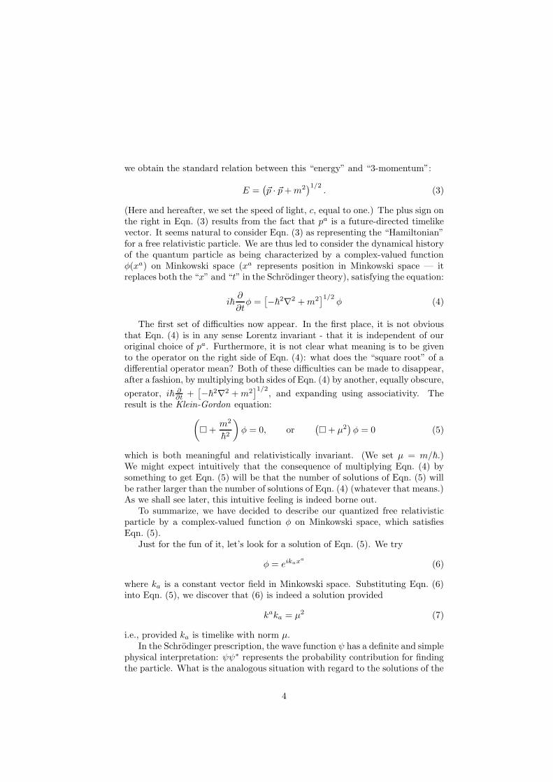
we obtain the standard relation between this “energy” and “3-momentum”:

E =(~p · ~p+m2

)1/2. (3)

(Here and hereafter, we set the speed of light, c, equal to one.) The plus sign onthe right in Eqn. (3) results from the fact that pa is a future-directed timelikevector. It seems natural to consider Eqn. (3) as representing the “Hamiltonian”for a free relativistic particle. We are thus led to consider the dynamical historyof the quantum particle as being characterized by a complex-valued functionφ(xa) on Minkowski space (xa represents position in Minkowski space — itreplaces both the “x” and “t” in the Schrodinger theory), satisfying the equation:

i~∂

∂tφ =

[−~2∇2 +m2

]1/2φ (4)

The first set of difficulties now appear. In the first place, it is not obviousthat Eqn. (4) is in any sense Lorentz invariant - that it is independent of ouroriginal choice of pa. Furthermore, it is not clear what meaning is to be givento the operator on the right side of Eqn. (4): what does the “square root” of adifferential operator mean? Both of these difficulties can be made to disappear,after a fashion, by multiplying both sides of Eqn. (4) by another, equally obscure,

operator, i~ ∂∂t +[−~2∇2 +m2

]1/2, and expanding using associativity. The

result is the Klein-Gordon equation:

(�+

m2

~2

)φ = 0, or

(�+ µ2

)φ = 0 (5)

which is both meaningful and relativistically invariant. (We set µ = m/~.)We might expect intuitively that the consequence of multiplying Eqn. (4) bysomething to get Eqn. (5) will be that the number of solutions of Eqn. (5) willbe rather larger than the number of solutions of Eqn. (4) (whatever that means.)As we shall see later, this intuitive feeling is indeed borne out.

To summarize, we have decided to describe our quantized free relativisticparticle by a complex-valued function φ on Minkowski space, which satisfiesEqn. (5).

Just for the fun of it, let’s look for a solution of Eqn. (5). We try

φ = eikaxa

(6)

where ka is a constant vector field in Minkowski space. Substituting Eqn. (6)into Eqn. (5), we discover that (6) is indeed a solution provided

kaka = µ2 (7)

i.e., provided ka is timelike with norm µ.In the Schrodinger prescription, the wave function ψ has a definite and simple

physical interpretation: ψψ∗ represents the probability contribution for findingthe particle. What is the analogous situation with regard to the solutions of the

4

Klein-Gordon equation? We know, e.g., from electrodynamics, that what is a“density” in a nonrelativistic theory normally becomes ”the time-component ofa 4-vector” in a relativistic theory. Thus, to replace “ψψ∗”, we are led to lookfor some 4-vector constructed out of a solution of the Klein-Gordon equation.This suggestion is further strengthened by the observation that for a Schrodingerparticle in a potential (so H = (1/2m)p2 + V (x)), we have the equation

∂

∂t(ψψ∗) = −~∇ ·

[~

2mi

(ψ∗~∇ψ − ψ~∇ψ∗

)](8)

(Proof: evaluate the time-derivatives on the left using (2), and verify that theresult is the same as the expression on the right.) This looks very much likethe nonrelativistic form of the statement that the 4-divergence of some 4-vectorvanishes. Hence, we want to construct some divergence-free 4-vector from solu-tions of the Klein-Gordon equation. One soon discovers such an object which,in fact, looks suggestively like the object appearing in Eqn. (8):

Ja =1

2i(φ∗∇aφ− φ∇aφ∗) (9)

Note that, because of (5), Ja is divergence-free.We cannot interpret the “time-component” of Eqn. (9) as a probability den-

sity for the particle unless this quantity is always nonnegative, that is to say,that Jat

a ≥ 0 for every future-directed timelike vector ta, that is to say, unlessJa itself is future-directed and timelike. To see whether this is indeed the case,we evaluate Ja for the plane-wave solution (Eqn. (6)), and find:

Ja = ka (10)

This expression is indeed timelike, but is not necessarily future-directed:Eqn. (6) is a solution of the Klein-Gordon equation whether ka is future- or past-directed. Thus, we have not succeeded in interpreting a solution of the Klein-Gordon equation in terms of a “probability density for finding the particle.”

We next consider the situation with regard to the initial value problem.Since the Schrodinger equation is first order in time derivatives, a solution of thatequation is uniquely specified by giving ψ′(x) at some initial time, say t = 0. TheKlein-Gordon equation, on the other hand, is second order in time derivatives.Hence, to specify a solution, one must give both φ and ∂φ/∂t at the initialtime t = 0. This radical change in the structure of the initial data is clearlya consequence of our having “squared” Eqn. (4). It is still another indicationthat the transition to the relativistic case is not just a trivial application of theSchrodinger prescription.

Finally, let’s look briefly at the structure of the space of solutions of theKlein-Gordon equation. In the non-relativistic case, the space of solutions ofthe Schrodinger equation is a Hilbert space: it’s obviously a complex vectorspace, and we define the norm of the state ψ by:

‖ψ‖2 =

∫

t=const.

ψψ∗dV (11)

5

That the real number (11) is independent of the t = const. surface overwhich the integral is performed is a consequence of Eqn. (8) (assuming, as onealways does, that ψ falls off sufficiently quickly at infinity.) One might thereforebe tempted to try to define the norm of a solution of the Klein-Gordon equationas an integral of Ja ∫

S

Jadsa (12)

over a spacelike 3-plane S. But it is clear from (10) that the expression (12) willnot in general be nonnegative. Thus, the most obvious way to make a Hilbertspace out of solutions of the Klein-Gordon equation fails. This, of course, israther embarrassing, for we are used to doing quantum theory in a Hilbertspace, with Hermitian operators representing observables, etc.

To summarize, a simple “relativization” of the Schrodinger equations leadsto a number of maladies.

2 Hilbert Space and Operators

The collection of states of a quantum system, together with certain of the struc-ture naturally induced on this collection, is described by a mathematical objectknown as a Hilbert space. We recall the basic definitions.

A Hilbert space consists, first of all, of a set H . Secondly, H has the structureof an Abelian group. That is to say, given any two elements, ξ and η, of H ,there is associated a third element of H , written ξ + η, this operation subjectto the following conditions:

H1. For ξ, η ∈ H , ξ + η = η + ξ.

H2. For ξ, η, φ ∈ H , (ξ + η) + φ = ξ + (η + φ).

H3. There is an element of H , written “0”, with the following property: foreach ξ ∈ H , ξ + 0 = ξ.

H4. If ξ ∈ H , there exists an element of H , written “−ξ”, with the followingproperty: ξ + (−ξ) = 0.

Furthermore, H has the structure of a complex vector space. That is to say,with each complex number α and each element ξ of H there is associated anelement of H , written αξ, this operation subject to the following conditions:

H5. For ξ, η ∈ H , α ∈ C, α(ξ + η) = αξ + αη.

H6. For ξ ∈ H , α, β ∈ C, (α+ β)ξ = αξ + βξ and (αβ)ξ = α(βξ).

H7. For ξ ∈ H , 1ξ = ξ.

There is, in addition, a positive-definite inner product defined on H . That is tosay, with any two elements, ξ and η, of H there is associated a complex number,written (ξ, η), this operation subject to the following conditions:

6

H8. For ξ, η, φ ∈ H , α ∈ C, (αξ + η, φ) = α(ξ, φ) + (η, φ).

H9. For ξ, η ∈ H , (ξ, η) = (η, ξ).

H10. For ξ ∈ H , with ξ 6= 0, (ξ, ξ) > 0. (That (ξ, ξ) is real follows from H9.)

We sometimes write ‖ξ‖ for√

(ξ, ξ). Finally, we require that this structure havea property called completeness. A sequence, ξi (i ∈ 1, 2, ...), of elements of H iscalled a Cauchy sequence if, for every number ε > 0, there is a number N suchthat ‖ξi − ξj‖ < ε whenever i and j are greater than N . A sequence is said toconverge to ξ ∈ H if ‖ξ − ξj‖ → 0 as i→∞. H is said to be complete if everyCauchy sequence converges to an element of H .

H11. H is complete.

There are, of course, hundreds of elementary properties of Hilbert spaces whichfollow directly from these eleven axioms.

A (linear) operator on a Hilbert space H is a rule A which assigns to eachelement ξ of H another element of H , written Aξ , this operation subject to thefollowing condition:

O1. ξ, η ∈ H , α ∈ C, A(αξ + η) = αAξ +Aη.

We shall discuss the various properties and types of operators when they arise.There is a fundamental difficulty which arises when one attempts to use

this mathematical apparatus in physics. The “collection of quantum states”which arises naturally in a physical problem normally satisfies H1–H10. (Thisis usually easy to show in each case.) The problem is with H11. The mostobvious collection of states often fails to satisfy the completeness condition. Asone wants a Hilbert space, he normally corrects this deficiency by completing thespace, that is, by including additional elements so that all Cauchy sequences willhave something to converge to. (There is a well-defined mathematical procedurefor constructing, from a space which satisfies H1–H10, a Hilbert space.) Theunpleasant consequence of being forced to introduce these additional states isthat the natural operators of the problem, which were defined on the originalcollection of states, cannot be defined in any reasonable way on the entire Hilbertspace. Thus, they are not operators at all as we have defined them, for theyonly operate on a subset of the Hilbert space. Fortunately, this subset is dense.(A subset D of a Hilbert space H is said to be dense if, for every element ξof H , there is a sequence consisting of elements of D which converges to ξ. )Some very unaesthetic mathematical techniques have been devised for dealingwith such situations. (See Von Neumann’s book on Mathematical Foundationsof Quantum Mechanics.)

This problem is not confined to quantum field theory. It occurs alreadyin Schrodinger theory. For example, the collection of smooth solutions of theSchrodinger equation for which the integral (11) converges satisfy H1–H10, butnot H11. To complete this space, we have to introduce “solutions” which are,for example, discontinuous. How does one apply the Schrodinger momentumoperator to such a wave function?

7

Figure 1: The mass shell in momentum space.

3 Positive-Frequency Solutions of the Klein-

Gordon Equation

We represent solutions of the Klein-Gordon equation as linear combinations ofplane-wave solutions (Eqn. (6)):

φ(x) =

∫

Mµ

f(ka)eikaxa

dVµ (13)

Of course, we wish to include in the integral (13) only plane-waves which satisfythe Klein-Gordon equation, i.e., only plane waves whose ka satisfy the nor-malization condition (7). The four-dimensional (real) vector space of constantvector fields in Minkowski space-time is called momentum space. The collectionof all vectors ka in momentum space which satisfy Eqn. (7) consists of two hy-perbolas (except in the case µ = 0, in which case the hyperbolas degenerate tothe two null cones through the origin). This collection is called the mass shell(associated with µ), Mµ (Fig. 1). Thus the function f in (13) is defined onlyon the mass shell, and the integral is to be carried out over the mass shell. Itis convenient, furthermore, to distinguish the future mass shell M+

µ (consist-ing of future-directed vectors which satisfy (7)) and the past mass shell M−µ(consisting of past-directed vectors which satisfy (7)), so Mµ = M+

µ ∪M−µ .Eqn. (13) immediately suggests two questions: i) What are the necessary

and sufficient conditions on the complex-valued function f on Mµ in order thatthe integral (13) exist for every xa, and in order that the resulting φ(x) besmooth and satisfy the Klein-Gordon equation? ii) What are the necessaryand sufficient conditions on a solution φ(x) of the Klein-Gordon equation in

8

Figure 2: The volume element on the mass shell.

order that it can be expressed in the form (13) for some f? These, of course,are questions in the theory of Fourier analysis. It suffices for our purposes,however, to remark that the required conditions are of a very general character(that functions not be too discontinuous, and that, asymptotically, they go tozero sufficiently quickly). The point is that all the serious things we shall do withthe Klein-Gordon equation will be in momentum space. We shall use MinkowskiSpace and φ(x) essentially only to motivate definitions and constructions on thef ’s in momentum space.

One question regarding (13) which must be answered is what is the volumeelement dVµ we are using on the mass shell. Of course, it doesn’t make anyreal difference, for a change in the choice of volume element would merely resultin a suitable readjustment of the f ’s. Our choice can therefore be dictated byconvenience. We require that our volume element be invariant under Lorentztransformations on momentum space (note that these leave the mass shell in-variant), and that it be applicable also in the case µ = 0. It is easy to state anappropriate volume element in geometrical terms. Let µ > 0. Then the massshell is a spacelike 3-surface in momentum space, in which there is a metric, so ametric is induced on Mµ. A metric on this 3-manifold defines a volume element

dVµ. This dVµ is clearly Lorentz-invariant, but, unfortunately, it approacheszero as µ→ 0. To correct this, we define

dVµ = µ−1dVµ (14)

which is easily verified to he nonzero also on the null cone. In more conventionalterms, our volume-element can be described as follows. Choose a unit time-likevector ta in momentum space, and let S be the spacelike 3-plane perpendicularto ta. Then any small patch A on Mµ, located at the point ka, can be projectedalong ta to give a corresponding patch A′ on S (see Fig. 2.) Let dV ′µ be thevolume of A′ on S (using the usual volume element in the 3-space S). Our

9

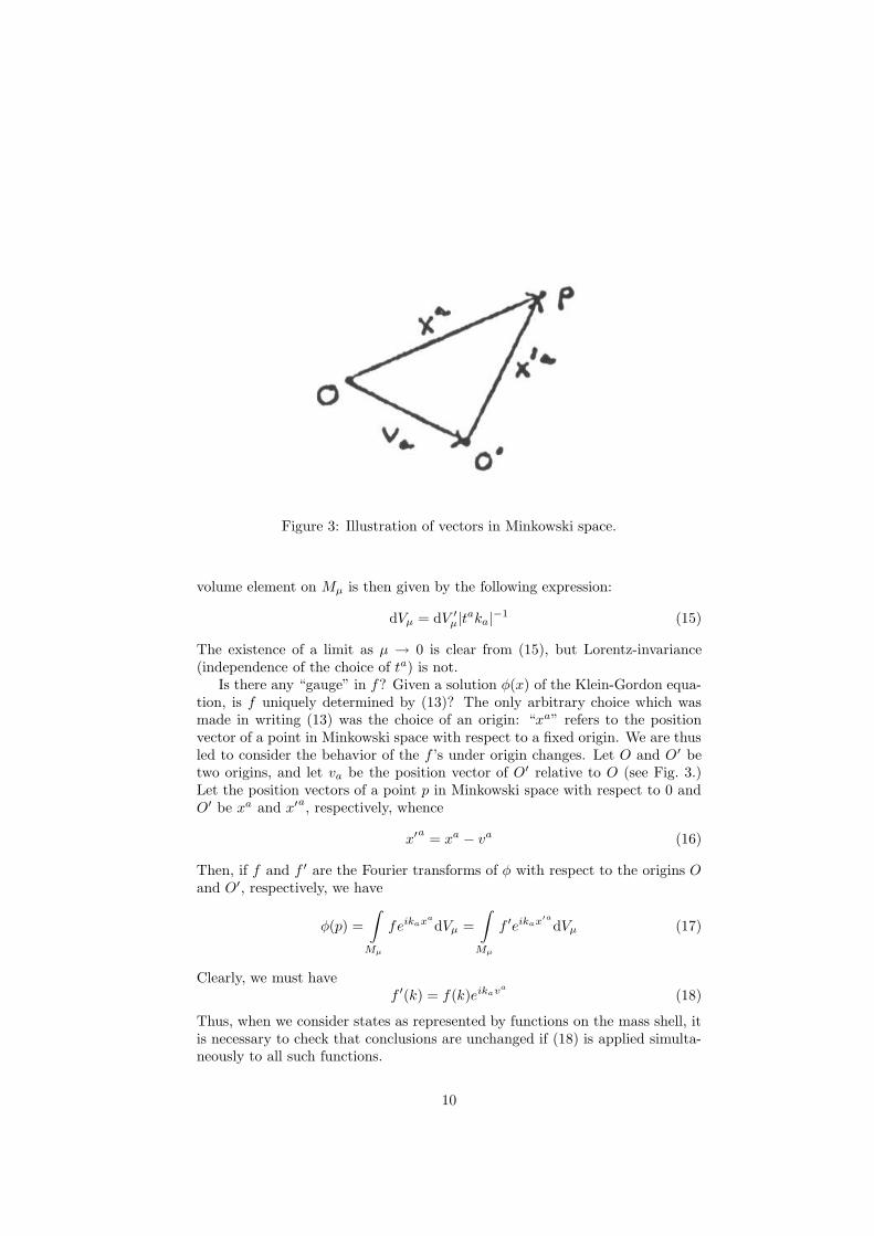
Figure 3: Illustration of vectors in Minkowski space.

volume element on Mµ is then given by the following expression:

dVµ = dV ′µ|taka|−1 (15)

The existence of a limit as µ → 0 is clear from (15), but Lorentz-invariance(independence of the choice of ta) is not.

Is there any “gauge” in f? Given a solution φ(x) of the Klein-Gordon equa-tion, is f uniquely determined by (13)? The only arbitrary choice which wasmade in writing (13) was the choice of an origin: “xa” refers to the positionvector of a point in Minkowski space with respect to a fixed origin. We are thusled to consider the behavior of the f ’s under origin changes. Let O and O′ betwo origins, and let va be the position vector of O′ relative to O (see Fig. 3.)Let the position vectors of a point p in Minkowski space with respect to 0 andO′ be xa and x′a, respectively, whence

x′a

= xa − va (16)

Then, if f and f ′ are the Fourier transforms of φ with respect to the origins Oand O′, respectively, we have

φ(p) =

∫

Mµ

feikaxa

dVµ =

∫

Mµ

f ′eikax′a

dVµ (17)

Clearly, we must havef ′(k) = f(k)eikav

a

(18)

Thus, when we consider states as represented by functions on the mass shell, itis necessary to check that conclusions are unchanged if (18) is applied simulta-neously to all such functions.

10

Now look again at Eqn. (3). It says, in particular, that the energy-momen-tum vector is future-directed. This same feature shows up in the right side ofEqn. (4) by the plus sign. If this sign were replaced by a minus, we would be deal-ing with a past-directed energy-momentum vector. The trick we used to obtainEqn. (5) from (4) amounted to admitting also past-directed energy-momenta.It is clear now how Eqn. (4) itself can be carried over into a well-defined andfully relativistic condition on φ. We merely require that the f of Eqn. (13) van-ish on M−µ . We call the corresponding solutions of the Klein-Gordon equationpositive-frequency (or positive-energy) solutions. Defining negative-frequencysolutions analogously, it is clear that every solution of the Klein-Gordon equation(more precisely, every solution which can be Fourier-analyzed) can be writtenuniquely as the sum of a positive-frequency and a negative-frequency solution.The positive-frequency solutions (resp., negative-frequency solutions) form avector subspace of the vector space of all (Fourier analyzable) solutions.

To summarize, we are led to take as the “wave function of a free relativistic(spin zero) particle” a positive-frequency solution of the Klein-Gordon equation.To what extent does this additional condition take care of the difficulties wediscovered in Sect. 1?

Consider first the current, Eqn. (9). We saw before, from the example ofa negative-frequency plane wave, that in general J is neither future-directedor even timelike. Is it true that J is future-directed timelike for a positive-frequency solution of the Klein-Gordon equation? Unfortunately, the answer isno. Consider a linear combination of two positive-frequency plane waves:

φ = eikaxa

+ αeik′axa

(19)

That is, α is a complex constant, and ka and k′a are future-directed constantvectors satisfying (7). (Strictly speaking, this example is not applicable, for (19)cannot be Fourier analyzed. It is not difficult, however, to appropriately smear(19) over the future mass shell to obtain an example without this deficiency.)Substituting (19) into (9), we obtain:

Ja =1

2ka

[2 + αei(k

′b−kb)xb + α∗ei(kb−k

′b)x

b]

+1

2k′a[2αα∗ + αei(k

′b−kb)xb + α∗ei(kb−k

′b)x

b] (20)

Clearly, one can choose α, ka, and k′a so that this Ja is not timelike in cer-tain regions. Thus, even the assumption of positive-frequency solutions doesnot resolve the difficulty associated with not having a simple probabilistic in-terpretation for our wavefunction φ: we still cannot think of Jat

a (with ta unit,future-directed, timelike) as representing a probability density for finding theparticle. The resolution of this problem must await our introduction of a posi-tion operator.

Note from Eqn. (20) that Ja is trying very hard to be timelike and future-directed in the positive-frequency case: it is only the cross terms between thetwo plane waves which destroys this property. This observation suggests that, in

11

the positive-frequency case, the integral of Ja over a spacelike 3-plane might bepositive. In order to check on this possibility, we want to rewrite the integral ofJa in terms of the corresponding function f on Mµ. It will be more illuminatingto do this for the general solution φ of the Klein-Gordon equation, i.e., notassuming, for the time being, that φ is positive-frequency. Substituting (13)into (9):

Ja =

∫

Mµ

dVµ

∫

Mµ

dV ′µ1

2k′a[f∗(k)f(k′)ei(k

′b−kb)xb + f(k)f∗(k′)ei(kb−k

′b)x

b]

(21)

We now let S be a spacelike 3-plane through the origin, and let ta be the unit,future-directed normal to S. Then

∫

S

Jata dS =

∫

Mµ

dVµ

∫

Mµ

dV ′µ1

2k′at

a

f∗(k)f(k′)

∫

S

ei(k′b−kb)xb dS

+f(k)f∗(k′)∫

S

ei(kb−k′b)x

b

dS

(22)

But, from the theory of Fourier analysis

∫

S

ei(k′b−kb)xb dS = (2π)3|taka|−1δ(k − k′) (23)

and so (22) becomes

∫

S

Jata dS = (2π)3

∫

M+µ

ff∗ dVµ −∫

M−µ

ff∗ dVµ

(24)

In particular, if f vanishes on M−µ , the left side of (24) must be positive, orvanishes if and only if φ vanishes. (The actual form of (24) was rather suggestedby Eqn. (15). If we had omitted the absolute-value sign on the right (and whatbetter thing could be done with an absolute-value sign?), the “volume element”on M−µ would have been negative.) This calculation was not done merely foridle curiosity; the right side of (24) will be important later.

We saw before that the initial-value problem for the Klein-Gordon equationis as follows: one must specify φ and ta∇aφ on an initial spacelike 3-plane. Howdoes the initial-value problem go for positive-frequency solutions of the Klein-Gordon equation? In fact, we only have to specify φ as initial data in this case.To see this, suppose we know the value of the integral

φ(x) =

∫

M+µ

f(k)eikaxa

dVµ (25)

12

for every xa which is perpendicular to a unit timelike vector ta at the origin(i.e., on the spacelike 3-plane perpendicular to ta, through the origin). Theintegral (25) can certainly be expressed as a Fourier integral over S (ta setsup a one-to-one correspondence between M+

µ and S). But then, by taking aFourier transform, we can determine f on M+

µ . Thus, we know φ throughoutMinkowski space. That is to say, when we properly interpret (4), we obtain a“Schrodinger-type” initial-value problem. If we ignore questions of smoothnessand convergence of Fourier integrals, the situation can be roughly summarizedas follows:

1. There is a one-to-one correspondence between: i) solutions of the Klein-Gordon equation, ii) complex-valued functions f on Mµ, and iii) values ofφ and ta∇aφ on a spacelike 3-plane.

2. There is a one-to-one correspondence between: i) positive-frequency solu-tions of the Klein-Gordon equation, ii) complex-valued functions on M+

µ ,and iii) values of φ on a spacelike 3-plane.

4 Constructing Hilbert Spaces and Operators

There is a general and extremely useful technique for obtaining a Hilbert spacealong with a collection of operators on it. It is essentially this technique whichis used, for example, in treating the Schrodinger and Klein-Gordon equations.It is convenient, therefore, to describe this construction, once and for all, in ageneral case. Special cases can then be treated as they arise.

The fundamental object we need is some n-dimensional manifold M onwhich there is specified a smooth, nowhere-vanishing volume-element dV . Indifferential-geometric terms, this means that we have a smooth, nowhere-vani-shing, totally skew tensor field εa1···an on M . Our Hilbert space, and operators,are now defined in terms of certain fields on M .

We first define the Hilbert space. Consider the collection H of all complex-valued, measurable, square-integrable functions f on M . This H is certainly acomplex vector apace. We introduce a norm on H :

‖f‖2 =

∫

M

ff∗ dV (26)

It is known that this H thus becomes a Hilbert space. (Actually, we havebeen a little sloppy here. One should, more properly, define an equivalencerelation on H : two functions are equivalent if they differ only on a subset (ofM) of measure zero. It is the equivalence classes which actually form a Hilbertspace. For example, the function f which vanishes everywhere on M except onepoint, where it is one, is measurable and square-integrable. Its norm, (26), iszero, although this f is not the zero element of H . It is, however, in the zeroequivalence class, for it differs from the zero function only on a set (namely, onepoint) of measure zero.) This is a special case of a more general theorem: the

13

collection of all complex-valued, measurable, square-integrable functions (moreprecisely, the collection of equivalence classes as above) on a complete measurespace form a Hilbert space.

We now introduce some operators. Let va be any smooth (complex) con-travariant vector field, and v any smooth (complex) scalar field on M . Thenwith each smooth, complex-valued function f on M we may associate the func-tion

V f = va∇af + vf (27)

where ∇a denotes the gradient on M . To what extent does (27) define anoperator on H? Unfortunately, (27) is not applicable to every element of H ,for two reasons: i) a function f could be measurable and square-integrable (i.e.,an element of H), but not differentiable. Then the gradient operation in (27)would not be defined. ii) an element f of H could even be smooth, but couldhave the property that, although f itself is square-integrable, the function (27)is not. However, there is a large class of elements of H on which (27) is definedand results in an element of H . Such a class, for example, is the collection ofall functions F which are smooth and have compact support. (Such a functionis automatically square-integrable and measurable.) This class is, in fact, densein H . Clearly, (27) is linear whenever it is defined. Thus, we can call (27) an“operator on H”, in the sense that we have agreed to abuse that term.

We agree to call an operator Hermitian if, whenever V f and V g are defined,(V f, g) = (f, V g). What are the necessary and sufficient conditions that (27)be Hermitian? Let f and g be smooth functions on M , of compact support.Then:

(V f, g) =

∫

M

(va∇af + vf)g∗ dV

=

∫

M

[−fva∇ag∗ + fg∗(−∇ava + v)] dV

(28)

where we have done an integration by parts (throwing away a surface term bythe compact supports). Eqn. (28) is clearly equal to

(f, V g) =

∫

M

[fv∗a∇ag∗ + fv∗g∗] dV (29)

for every f and g when and only when:

v∗a = −va v − v∗ = ∇ava (30)

These, then, are the necessary and sufficient conditions that V be Hermitian.One further remark is required with regard to what the divergence in the firstEqn. (30) is supposed to mean. (We don’t have a metric, or a covariant deriva-tive, defined on M .) It is well-known that the divergence of a contravariantvector field can be defined on a manifold with a volume-element εa1···an . This

14

can be done, for example, using either exterior derivatives or Lie derivatives.For instance, using Lie derivatives we define “∇ava” by:

Lvmεa1···an = (∇ava)εa1···an (31)

(Note that, since the left side is totally skew, it must be some multiple ofεa1···an .)

Finally, we work out the commutator of two of our operators; V = (va, v)and W = (wa, w). If f is a smooth function of compact support, we have:

[V,W ]f = (va∇a + v)(wb∇b + w)f − (wb∇b + w)(va∇a + v)f

= (vb∇bwa − wb∇bva)∇af + (va∇aw − wa∇av)f(32)

Note that the commutator is again an operator of the form we have been dis-cussing, (27). Note furthermore that the vector part of the commutator is theLie bracket of the vector fields appearing in V and W .

To summarize, with any n-manifold M on which there is given a smooth,nowhere-vanishing volume element we associate a Hilbert space H along with acollection of operators on H . The commutator of two operators in this collectionis again an operator in the collection.

5 Hilbert Space and Operators for the Klein-

Gordon Equation

We now complete our description of the quantum theory of a free, relativistic,spin-zero particle.

For our Hilbert space we take, as suggested by Sec. 3, the collection ofall complex-valued, measurable, square-integrable functions on the future massshell, M+

µ . In order to obtain position, momentum, energy, etc. operators, weuse the scheme described in Sec. 4. That is, we look for vector and scalar fieldson M+

µ .We first consider momentum operators. Let pa be any constant vector field

in Minkowski apace, and φ any positive-frequency solution of the Klein-Gordonequation. Then, clearly,

~ipa∇aφ (33)

is also a positive-frequency solution of the Klein-Gordon equation. In terms ofthe corresponding functions on M+

µ , (33) takes the form

f → (~paka)f (34)

That is to say, we multiply f by the real function (~paka) on M+µ . Thus, for

each constant vector field pa, we have an operator, P (pa), on our Hilbert spaceH . Since the multiplying function in (34) is real, the operators P (pa) are allHermitian. (See (30).) We now interpret these operators. Choose a constant,

15

unit, future-directed timelike vector field ta in Minkowski space (a preferred“state of rest”). Then P (ta) is the “energy” operator, and P (pa), with pa unitand perpendicular to ta, is the “component of momentum in the pa-direction”operator.

The position operators are more complicated. Not only do they depend onmore objects in Minkowski space (rather than just a single pa as in the momen-tum case), but also they require us to take derivatives in the mass shell. Toobtain a position operator, we need the following information: a choice of originO in Minkowski space, a constant, unit, future-directed timelike vector field ta

in Minkowski space, and a constant unit vector field qa which is perpendicularto ta. (Roughly speaking, O and ta define a spacelike 3-plane — the “instant”at which the operator is to be applied — qa defines “which position coordinatewe’re operating with”, and O tells us what the origin of this position coordinateis.) Now, qa is a vector in momentum space, and therefore defines a constantvector field in momentum space, which we also write as qa. One is tempted totake the derivative of f along this vector field. But this will not work, for qa isnot tangent to the mass shell, whereas f is only defined on the mass shell. Tocorrect this deficiency, we project qa into the mass shell — that is, we add toqa that multiple of ta which results in a vector field lying in M+

µ :

−1

i

[qa − ta(tbkb)

−1(qckc)]

(35)

We now have a vector field on M+µ , and therefore an operator on our Hilbert

space H . But are those operators Hermitian? From (30), we see that thisquestion reduces to the question of whether the divergence of (35) vanishes ornot. Unfortunately, we obtain for this divergence

−1

i

(gab − µ−2kakb

)∂a[qb − tb(tckc)−1(qdkd)

]= −1

i(qaka)(tbkb)

−2 (36)

where we have denoted the derivative in momentum space by ∂a. To obtain aHermitian operator, we take the Hermitian part of the operator represented by(35):

f → −1

i

[qa − ta(tbkb)

−1(qckc)]∂af −

1

2i(qaka)(tbkb)

−2 (37)

In (37), f is to be the function on M+µ obtained using O as the origin (see

(18).) (Why is there no ~ in (37)? We should, perhaps, have called k-space“wave number and frequency space” rather than “momentum space”.) We shallwrite the operator (37) X(O, ta, qa). For any value of its arguments, X is aHermitian operator on H . (It is strange — and perhaps rather unpleasant —that the position and momentum operators are so different from each other.)

We now have a lot of operators, and so we can ask for their commutators.This is easily done by substituting into our explicit formula, Eqn. (32). The

16

result is the standard formulae:[P (pa), P (p′

a)]

= 0[X(O, ta, qa), X(O, ta, q′

a)]

= 0

[P (pa), X(O, ta, qa)] = −i~(paqa)

(pata) = 0

(38)

The next thing one normally does with operators (in the Heisenberg repre-sentation, which is the one we’re using) is to work out their time derivatives.For the momentum operators, this is easy, for no notion of a “time” was used todefine P (pa)). Thus, whatever reasonable thing one wants to mean by a “ ˙ ”,we have:

P (pa) = 0 (39)

This, of course, is what we expect for the momentum operator on a free particle.For the position operators, on the other hand, we have an interesting notionof time-derivative. We want to compare X(O, ta, qa) with “the same positionoperator at a slightly later time”. This “at a slightly later time” is expressedby slightly displacing O in the ta-direction. Thus, we are led to define:

X(O, ta, qa) = limε→0

1

ε[X(O′, ta, qa)−X(O, ta, qa)] (40)

where O′ is defined by the property that its position vector relative to O is εta.It is straightforward to check, with this definition, that

X(O, ta, qa)f = −(qaka)(tbkb)−1f (41)

which, of course, is what we expected. Note that a number of statements abouthow X(O, ta, qa) depends on its arguments follow directly from Eqn. (41).

Finally, one would like to ask about the eigenvectors and eigenvalues of ouroperators. It is clear from Eqn. (34) that the only candidate for an eigenfunc-tion of P (pa) would be a δ-function on M+

µ . Of course, a δ-function is not afunction, and hence not an element of H (we cannot enlarge H to include suchfunctions, if we want to keep a Hilbert space, for a δ-function should not besquare-integrable.) It is convenient to have the idea, however, that if P (pa)had eigenfunctions, they would be plane-waves. We next ask for eigenfunctionsof X(O, ta, qa). We look for the wave function of a “particle localized at theorigin”, that is we look for an f such that X(O, ta, qa)f = 0 for every qa whichis perpendicular to ta (ta and O fixed). That is, from (37), we require that

[qa − ta(tbkb)

−1(qckc)]∂af −

1

2(qaka)(tbkb)

−2f = 0 (42)

for every such qa. The solution to (42) is:

f = const. (taka)1/2 (43)

The first remark concerning (43) is that it is not square-integrable, and hencedoes not represent an element of H . This does not stop us, however, from

17

substituting (43) into (13) to obtain a function φ on Minkowski space. Theresulting φ (the explicit formula is not very enlightening — it involves Hankelfunctions) is not a δ-function at O. In fact, this φ is “spread out” around O todistances of the order of µ−1 — the Compton wavelength of our particle. Thus,our picture is that a relativistic particle cannot be confined to distances muchsmaller than its Compton wavelength.

6 The Direct Sum of Hilbert Spaces

Associated with any countable sequence, H ′, H ′′, H ′′′, . . ., of Hilbert spaces thereis another Hilbert space, written H ′⊕H ′′⊕H ′′′⊕ . . ., and called the direct sumof H ′, H ′′, H ′′′, . . .. We shall give the definition of the direct sum and a few ofits elementary properties.

Consider the collection of all sequences

(ξ′, ξ′′, ξ′′′, . . .) (44)

consisting of one element (ξ′) of H ′, one element (ξ′′) of H ′′, etc., for which thesum

‖ξ′‖2 + ‖ξ′′‖2 + ‖ξ′′‖2 + . . . (45)

converges. This collection is the underlying point set of the direct sum. Toobtain a Hilbert space, we must define addition, scalar multiplication, and aninner product, and verify H1–H11.

The sum of two sequences (44) is defined by adding them “component-wise”:

(ξ′, ξ′′, ξ′′′, . . .) + (η′, η′′, η′′′, . . .) = (ξ′ + η′, ξ′′ + η′′, ξ′′′ + η′′′, . . .) (46)

We must verify that, if the addends satisfy (45), then so does the sum. Thisfollows immediately from the inequality:

‖ξ′ + η′‖2 = ‖ξ′‖2 + (ξ′, η′) + (η′, ξ′) + ‖η′‖2

≤ ‖ξ′‖2 + 2‖ξ′‖‖η′‖+ ‖η′‖2

≤ 2‖ξ′‖2 + 2‖η′‖2(47)

The product of a sequence (44) and a complex number α is defined by:

α(ξ′, ξ′′, ξ′′′, . . .) = (αξ′, αξ′′, αξ′′′, . . .) (48)

That the right side of (48) satisfies (45) follows from the fact that

‖αξ′‖ = |α|‖ξ′‖ (49)

We have now defined addition and scalar multiplication. That these two oper-ations satisfy H1–H7, i.e., that we have a complex vector space, is trivial.

We define the inner product between two sequences (44) to be the complexnumber

((ξ′, ξ′′, ξ′′′, . . .), (η′, η′′, η′′′, . . .)) = (ξ′, η′) + (ξ′′, η′′) + (ξ′′, η′′) + . . . (50)

18

The indicated sum of complex numbers on the right of (50) converges if (in fart,converges absolutely if and only if) the sum of the absolute values converges.Thus, the absolute convergence of the right side of (50) follows from the factthat

|(ξ′, η′)| ≤ ‖ξ′‖ ≤ 1

2‖ξ′‖2 +

1

2‖η′‖2 (51)

We now have a complex vector space in which there is defined an inner product.(Note incidentally, that the norm is given by (45).) The verification of H8, H9,and H10 is easy.

Thus, as usual, the only difficult part is to check H11. Consider a Cauchysequence of sequences (44). That is to say, we have a countable collection ofsuch sequences,

φ1 = (ξ′1, ξ′′1 , ξ′′′1 , . . .)

φ2 = (ξ′2, ξ′′2 , ξ′′′2 , . . .)

φ3 = (ξ′3, ξ′′3 , ξ′′′3 , . . .)

...

(52)

with the following property: for each real ε > 0 there is a number N such that

‖φi − φj‖2 = ‖ξ′i − ξ′j‖2 + ‖ξ′′i − ξ′′j ‖2 + · · · ≤ ε (53)

whenever i, j ≥ N . We must show that the sequence of elements (52) of thedirect sum converge to some element of the direct sum. First note that (53)implies

‖ξ′i − ξ′j‖2 ≤ ε, ‖ξ′′i − ξ′′j ‖2 ≤ ε, . . . (54)

That is to say, the first “column” of (52) is a Cauchy sequence in H ′, the secondcolumn a Cauchy sequence in H ′′, etc. Since H ′, H ′′, . . . are Hilbert spaces,these Cauchy sequences converge, say, to ξ′ ∈ H ′, ξ′′ ∈ H ′′, etc. Form

φ = (ξ′, ξ′′, ξ′′′, . . .) (55)

We must show that the φi converge to φ, and that is φ is an element of thedirect sum (i.e., that (45) converges for φ). Fix ε ≥ 0 and choose i such that‖φi − φj‖2 ≤ ε whenever j > i. Then, for each positive integer n,

‖ξ′i − ξ′j‖2 + ‖ξ′′i − ξ′′j ‖2 + . . .+ ‖ξ(n)i − ξ(n)

j ‖2 ≤ ε (56)

Taking the limit of (56) as j →∞, we obtain

‖ξ′i − ξ′‖2 + ‖ξ′′i − ξ′′‖2 + . . .+ ‖ξ(n)i − ξ(n)‖2 ≤ ε (57)

but n is arbitrary, and so, taking the limit of (57) as n→∞,

‖φi − φ‖2 = ‖ξ′i − ξ′‖2 + ‖ξ′′i − ξ′′‖2 + . . . ≤ ε (58)

19

That is to say, the φi converge to φ. Finally, the fact that φ is actually anelement of the direct sum, i.e., the fact that

‖ξ′‖2 + ‖ξ′′‖2 + ‖ξ′′‖2 + . . . (59)

converges, follows immediately by substituting

‖ξ′‖2 ≤ 2‖ξ′i‖2 + 2‖ξ′i − ξ′‖2 (60)

(and the corresponding expressions with more primes) into (59), and using (58)and the fact that φi is an element of the direct sum. Thus, the direct sum iscomplete.

To summarize, we have shown how to construct a Hilbert space from acountable sequence of Hilbert spaces. Note, incidentally, that the direct sumis essentially independent of the order in which the Hilbert spaces are taken.More precisely, the direct sum obtained by taking H ′, H ′′, . . . in one order isnaturally isomorphic to the direct sum obtained by taking these spaces in anyother order.

Finally, we discuss certain operators on the direct sum. Consider a sequenceof operators: A′ acting on H ′, A′′ acting on H ′′, etc. Then with each element(44) of the direct sum we may associate the sequence

(A′ξ′, A′′ξ′′, A′′′ξ′′′, . . .) (61)

Unfortunately, (61) may not be an element of the direct sum, for

‖A′ξ′‖2 + ‖A′′ξ′′‖2 + ‖A′′′ξ′′′‖2 + . . . (62)

may fail to converge. However, (61) will produce an element of the direct sumwhen acting on a certain dense subset of the direct sum, namely, the set ofsequences (44) which consist of zeros after a certain point. Is there any conditionon the A’s which will ensure that (61) will always be an element of the directsum? An operator A on a Hilbert space H is said to be bounded if A is definedeverywhere and, for some number a, ‖Aξ‖ ≤ a‖ξ‖ for every ξ ∈ H . Thesmallest such a is called the bound of A, written |A|. (The norm on a Hilbertspace induces on it a metric topology. Boundedness is equivalent to continuityin this topology.) It is clear that (62) converges for every element of the directsum provided i) all the A’s are bounded, and ii) the sequence of real numbers|A′|, |A′′|, . . . is bounded.

7 The Completion of an Inner-Product Space

It is sometimes the case, when one wishes to construct a Hilbert space, that onefinds a set on which addition, scalar multiplication, and an inner product aredefined, subject to H1–H10 — what we shall call an inner product space. Onewants, however, to obtain a Hilbert space, i.e., something which also satisfies

20

H11. There is a construction for obtaining a Hilbert space from an inner prod-uct space. Since this construction is in most textbooks, we merely indicate thegeneral idea.

Let G be an inner product space. Denote by G′ the collection of all Cauchysequences in G′. If ξi ∈ G′, ηi ∈ G′ (i = 1, 2, . . .), we write ξi ≈ ηi provided

limi→∞

‖ξi − ηi‖ = 0 (63)

One verifies that “≈” is an equivalence relation. The collection of equivalenceclasses, denoted by G, is to be made into a Hilbert space.

Consider two elements of G, i.e., two equivalence classes, and let ξi and ηibe representatives. We define a new sequence, whose ith element is ξi + ηi.One verifies, using the fact that ξi and ηi, are Cauchy sequences, that this newsequence is also Cauchy. Furthermore, if ξi and ηi are replaced by equivalentCauchy sequences, the sum becomes a Cauchy sequence which is equivalent toξi + ηi. Thus, we have defined an operation of addition in G. In addition, ifξi is a Cauchy sequence and α a complex number, αξi is a Cauchy sequencewhose equivalence class depends only on the equivalence class of ξi. We havethus defined an operation of scalar multiplication in G. These two operationssatisfy H1–H7.

If ξi ∈ G′, ηi ∈ G′, thenlimi→∞

(ξi, ηi) (64)

exists. Furthermore, this complex number is unchanged if ξi and ηi are replacedby equivalent Cauchy sequences. Thus, (64) defines an inner product on G. One

must now verify H8, H9, and H10, so that G becomes an inner product space.Finally (and this is the only hard part), one proves that G is complete, and so

constitutes a Hilbert space. The Hilbert space G is called the completion of theinner product space G.

Note that G can be considered as a subspace of its completion; with eachξ ∈ G associate the element of G (the equivalence class) containing the Cauchysequence ξi = ξ of G. It is easily checked from the definition, in fact, that G isdense in G. Suppose that G itself were already complete? Then every Cauchysequence in G would converge, and, from (63), two Cauchy sequences would beequivalent if and only if they converged to the same thing. Thus, in this caseG would be just another copy of G; the completion of a complete space is justthat space again.

Finally, suppose that A is a bounded operator on the inner product spaceG. Then A can be extended to a bounded operator on G. That is, there is abounded operator on G which reduces to A on G considered as a subspace ofG. To prove this, let ξi be a Cauchy sequence in G. Then, since A is bounded,

‖Aξi −Aξj‖ = ‖A(ξi − ξj)‖ ≤ |A|‖ξi − ξj‖ (65)

whence Aξi is a Cauchy sequence in G. Furthermore, if two Cauchy sequencessatisfy (63), then

limi→∞

‖Aξi −Aηi‖ ≤ |A| limi→∞

‖ξi − ηi‖ = 0 (66)

21

That is to say, Aξi is replaced by an equivalent Cauchy sequence when ξi is.Therefore, we can consider A as acting on elements of G to produce elementsof G. This action is clearly linear, and so we have an operator A defined on G.Furthermore, this A is bounded, and in fact |A| = |A|, for

limi→∞

‖Aξi‖ ≤ |A| limi→∞

‖ξi‖ (67)

for any Cauchy sequence in G.

8 The Complex-Conjugate Space of a HilbertSpace

Let H be a Hilbert space. We introduce the notion of the complex-conjugatespace of H , written H . As point-sets, H = H. That is to say, with eachelement ξ ∈ H there is associated an element of H; this element will be writtenξ. Furthermore, we take as the group structure on H that is induced from H :

ξ + η = (ξ + η) (68)

In other words, the sum of two elements of H is defined by taking the sum(in H) of the corresponding elements of H , and taking the result back to H .Scalar multiplication in H , on the other hand, is defined by the formula (µ ∈ C,ξ ∈ H):

µξ = (µξ) (69)

That is, to multiply an element of H by a complex number, one multipliesthe corresponding element of H by the complex-conjugate of that number, andtakes the result back to H. (Note that a bar appears in two different senses in(69). A bar over a complex number denotes its complex-conjugate; a bar overan element of H denotes the corresponding element of H .) Finally, the innerproduct on H is fixed by requiring that the transition from H to H preservenorms:

‖ξ‖ = ‖ξ‖ (70)

It is obvious that this H thus becomes a Hilbert space.Note that the complex-conjugate space of H is naturally isomorphic with

H . We write ¯H = H , and, for ξ ∈ H , ¯ξ = ξ.The reason for introducing H is that one frequently encounters mappings

on H which are anti-linear (T (µξ + η) = µT (ξ) + T (η)) rather than linear(T (µξ+η) = µT (ξ)+T (η)). Anti-linear mappings on H become linear mappingson H, and it is easier to think about linear mappings than anti-linear ones.Consider, for example, the inner product on H , (ξ, η). This can be consideredas a mapping H ×H → C, which is linear in the first H and anti-linear in thesecond. If, however, we consider the inner product as a mapping H × H → C,it becomes linear in both factors.

22

9 The Tensor Product of Hilbert Spaces

With any finite collection of Hilbert spaces, Hα, Hβ , . . . , Hγ , there is associatedanother Hilbert space, called the tensor product of Hα, Hβ, . . . , Hγ , and writtenHα⊗Hβ ⊗ · · · ⊗Hγ . We shell define the tensor product and derive a few of itsproperties.

It is convenient to introduce an index notation. We attach a raised Greekindex to a vector to indicate to which Hilbert space it belongs, e.g., ξα ∈ Hα,ηβ ∈ Hβ . The corresponding complex-conjugate spaces, Hα, Hβ, . . . , Hγ , willbe written Hα, Hβ, . . . , Hγ . Membership in the complex-conjugate spaces willbe indicated with a lowered Greek index. The element of Hα which correspondsto ξα ∈ Hα would be written ξα, while (69) would be written thus: µξα = (µ ξα).Finally, the operation of taking the inner product (which associates a complexnumber, linearly, with an element of H and an element of H) is indicated byplacing the two elements next to each other, e.g., ξαηα. Hence, ‖ξα‖2 = ξαξα.The inner product operation looks (and is) similar to “contraction.”

We now wish to define the tensor product. In order to avoid cumbersomestrings of dots, we shall discuss the tensor product of just two Hilbert spaces, Hα

and Hβ. The tensor product of n Hilbert spaces is easily obtained by insertingdots at appropriate places in the discussion below.

Consider the collection of all formal expressions of the following type:

ξαηβ + . . .+ σατβ (71)

“Formal” here means that the pluses and juxtapositions of elements in (71) arenot to be considered, for the moment, as well-defined operations. They aremerely marks on the paper. We introduce, on the collection of all such formalsums, an equivalence relation: two formal sums will be considered equivalentif they can be obtained from each other by any combination of the followingoperations on such sums:

1. Permute, in any way, the terms of a formal sum.

2. Add to a formal sum, or delete, the following combination of terms:(µξα)ηβ + (−ξα)(µ−1ηβ).

3. Add to a formal sum, or delete, the following combination of terms: (ξα+σα)ηβ + (−ξα)ηβ + (−σα)ηβ .

4. Add to a formal sum, or delete, the following combination of terms:ξα(ηβ + τβ) + ξα(−ηβ) + ξα(−τβ).

We denote the collection of equivalence classes by F αβ . The idea is to intro-duce on this Fαβ the structure of an inner-product space, and then take thecompletion to obtain the tensor product.

We add two formal sums by “stringing them together”:

(ξαηβ+. . .+σατβ)+(φαψβ+. . .+λακβ) = ξαηβ+. . .+σατβ+φαψβ+. . .+λακβ

(72)

23

The equivalence class of the formal sum on the right in (72) depends, ofcourse, only on the equivalence classes of the two formal sums on the left, andso we have defined an operation of addition on F αβ . Similarly, the product ofa format sum and a complex number, defined by

µ(ξαηβ + . . .+ σατβ) = (µξα)ηβ + . . .+ (µσα)τβ (73)

induces an operation of scalar multiplication on F αβ . (Note that we don’tchange the equivalence class of the right side of (73) by placing some or all ofthe µ’s with the second vectors rather than the first.) Thus, we have on F αβ

the structure of a complex vector space. So far, we have merely repeated thestandard construction of the tensor product of two vector spaces.

We next wish to define an inner product, or, equivalently, a norm, on F αβ .The norm of a formal sum, Eqn. (71), is defined by writing

(ξαηβ + · · ·+ σατβ)(ξαηβ + · · ·+ σατβ) (74)

and expanding using associativity. For example, the norm of a formal sum withjust two terms would be given by the sum of the complex numbers on the rightof:

(ξαηβ + σατβ)(ξαηβ + σατβ)

= (ξαξα)(ηβ ηβ) + (σαξα)(τβ ηβ) + (ξασα)(ηβ τβ) + (σασα)(τβ τβ)(75)

This norm clearly depends only on the equivalence class of the formal sum, andso defines a norm, and hence an inner product on F αβ . This inner producton Fαβ certainly satisfies H8 and H9 — but does it satisfy also H10? Toshow that it does involves a bit more work. A formal sum will be said to bein normal form if any two elements of Hα appearing in that sum are eitherproportional to each other (parallel) or have vanishing inner product with eachother (perpendicular) and if, furthermore, any two elements of Hβ appearing inthat sum are also either parallel or perpendicular, and if, finally, no two terms inthat sum have the property that both their Hα elements and their Hα elementsare parallel. (This last condition can always be achieved by combining terms.)The norm of a formal sum in normal form is clearly positive. For example, ifEqn. (71) were in normal form, its norm would be

∥∥ξαηβ + . . .+ σατβ∥∥2

= (ξαξα)(ηβ ηβ) + . . .+ (σασα)(τβ τβ) (76)

Thus, the proof that the norm we have defined on F αβ is positive-definite willbe complete if we can show that every formal sum is equivalent to a formal sumin normal form. The essential step in this demonstration is the Gram-Schmidtorthogonalization procedure. Let ξ, η1, . . . , ηn be elements of a Hilbert space H .Then

ξ = µ1η1 + · · ·+ µnηn + τ (µi ∈ C, (ηi, τ) = 0) (77)

That is to say, any vector in H can be written as a linear combination ofη1, . . . , ηn, plus a vector perpendicular to the η’s. Consider now a formal sum,say

ξαηβ + σατβ + φαψβ (78)

24

We obtain an equivalent formal sum by replacing σα by a vector parallel toξα plus a vector perpendicular to ξα and combining terms. Thus, Eqn. (78) isequivalent to a formal sum

ξαη′β

+ σ′ατβ + φαψβ (79)

in which σ′α is perpendicular to ξα. We next obtain an equivalent formal sumby replacing φα by a vector parallel to σ′α plus a vector parallel to ξα plus avector perpendicular to both σ′α and ξα. Thus, Eqn. (79) is equivalent to aformal sum

ξαη′′β

+ σ′ατ ′β

+ φ′αψβ (80)

with ξα, σ′α, and φ′α all perpendicular to each other. We now repeat thisprocedure with the Hβ vectors to obtain a formal sum in normal form which isequivalent to Eqn. (78). Hence, every formal sum is equivalent to a formal sumin normal form, whence the norm on F αβ is positive-definite, whence Fαβ is aninner-product space.

We now define the tensor product of Hα and Hβ to be the completion ofFαβ :

Hα ⊗Hβ = Fαβ (81)

This is really quite complicated. An element of the tensor product is an equiv-alence class of Cauchy sequences in an inner-product space whose elements areequivalence classes of formal sums. Note that F αβ itself can be considered asa subspace of Hα ⊗Hβ . Elements of the tensor product which belong to F αβ

will be called finite elements. In fact, we shall go one step further and considerformal sums (71) to be elements of the tensor product. Equivalent formal sumsare then equal as elements of the tensor product. With these conventions, weshall be able to avoid, for the most part, having to speak always in terms ofequivalence classes and Cauchy sequences.

The tensor product of more than two Hilbert spaces, Hα ⊗Hβ ⊗ · · · ⊗Hγ ,is defined in a completely analogous way. We use Greek indices to indicatemembership in the various tensor products, e.g., we write ξαβ···γ for a typicalelement of Hα ⊗Hβ ⊗ · · · ⊗Hγ . Addition and scalar multiplication within thetensor products is indicated in the obvious way:

ξαβ···γ + ηαβ···γ

µξαβ···γ(82)

Note, incidentally, that our original formal sums are now considerably less for-mal. For example, Eqn. (71) can be considered as the sum, in Hα ⊗Hβ, of thefollowing elements of Hα ⊗Hβ: ξαηβ , . . . , σατβ .

We next observe that there is a natural, one-to-one correspondence betweenthe formal sums which are used to obtain Hα ⊗ · · · ⊗Hβ ,

ξα · · · ηβ + · · ·+ σα · · · τβ (83)

25

and those which are used to obtain Hα ⊗ · · · ⊗ Hβ :

ξα · · · ηβ + · · ·+ σα · · · τβ (84)

That is to say, the inner product space consisting of finite elements of Hα ⊗· · · ⊗ Hβ is the complex conjugate space of the inner product space consistingof finite elements of Hα ⊗ · · · ⊗ Hβ . This relationship clearly continues tohold in the actual tensor product spaces. We conclude that Hα ⊗ · · · ⊗ Hβ isthe same as (words we shall frequently use instead of “is naturally isomorphic

with”) Hα ⊗ · · · ⊗Hβ . The tensor product of the complex-conjugate spaces isthe same as the complex-conjugate space of the tensor product. This fact allowsus to extend our index notation still further. A typical element of Hα⊗· · ·⊗Hβ

will be written ξα···β , this being the element which corresponds to the elementξα···β of Hα⊗ · · · ⊗Hβ . The inner product, in the tensor product space, of twoelements, ξα···β and ηα···β , of Hα ⊗ · · · ⊗Hβ can now be written as follows:

ξα···βηα···β (85)

Thus, the index notation extends very nicely from the original collection ofHilbert spaces to the various tensor products which can be constructed.

We now introduce some operations between elements of our tensor productspaces. Let ξα···βγ···δ and ηγ···δ be finite elements of Hα⊗. . .⊗Hβ⊗Hγ⊗. . .⊗Hγ

and Hγ ⊗ . . .⊗ Hδ , respectively. We can certainly associate with these two anelement, ξα···βγ···δ ηγ···δ of Hα ⊗ . . .⊗Hβ . For example,

(ξαηβσγτ δ + φαψβλγκδ)(ργ εδ + νγ ζδ)

= ξαηβ(σγ ργ)(τ δ εδ) + φαψβ(λγ ργ)(κδ εδ) + ξαηβ(σγ νγ)(τ δ ζδ)

+ φαψβ(λγ νγ)(κδ ζδ)

(86)

Note, furthermore, that

‖ξα···βγ···δ ηγ···δ‖ ≤ ‖ξα···βγ···δ‖‖ηγ···δ‖, (87)

a result which is easily checked by placing ξα···βγ···δ and ηγ···δ in normal form.Can this operation be extended from finite ξα···βγ···δ , ηγ···δ to the entire tensor

product? To see that it can, let ξα···βγ···δi and ηiγ···δ, be Cauchy sequences offinite elements of Hα⊗ . . .⊗Hβ⊗Hγ⊗ . . .⊗Hγ and Hγ⊗ . . .⊗Hδ, respectively.Then

‖ξα···δi ηiγ···δ − ξα···δj ηjγ···δ‖= ‖ξα···δi ηiγ···δ − ξα···δj ηiγ···δ + ξα···δj ηiγ···δ − ξα···δj ηjγ···δ‖≤ ‖ξα···δi − ξα···δj ‖‖ηiγ···δ‖+ ‖ξα···δj ‖‖ηiγ···δ − ηjγ···δ‖

(88)

where we have used (87). Thus, ξα···βγ···δηγ···δ is a Cauchy sequence in theHilbert space Hα⊗ . . .⊗Hβ; hence it converges to some element of this Hilbertspace. In this way, we associate with any (not necessarily finite) elements

26

ξα···βγ···δ and ηγ···δ an element ξα···βγ···δηγ···δ. This product is clearly linearin the factors, and satisfies (87). The operation of contraction is thus extendedfrom the Hilbert spaces to their tensor products. Note that (85) is now a specialcase.

Now let ξα···β and ηγ···δ be finite elements of Hα⊗. . .⊗Hβ and Hγ⊗. . .⊗Hδ,respectively. We can certainly associate with these two an element, ξα···βηγ···δ ,Hα ⊗ . . .⊗Hβ ⊗Hγ ⊗ . . .⊗Hδ. For example,

(ξαηβ +σατβ)(φγψδ +λγκδ) = ξαηβφγψδ +σατβφγψδ + ξαηβλγκδ +σατβλγκδ

(89)Note, furthermore, that

‖ξα···βηγ···δ‖ = ‖ξα···β‖‖ηγ···δ‖ (90)

This operation, too, can be extended from finite elements to the entire tensorproduct. Let ξα···βi and ηγ···δi be Cauchy sequences. Then ξα···βi ηγ···δi is also aCauchy sequence, for

‖ξα···βi ηγ···δi − ξα···βj ηγ···δj ‖= ‖ξα···βi ηγ···δi − ξα···βj ηγ···δi + ξα···βj ηγ···δi − ξα···βj ηγ···δj ‖≤ ‖ξα···βi − ξα···βj ‖‖ηγ···δi ‖+ ‖ξα···βj ‖‖ηγ···δi − ηγ···δj ‖

(91)

This Cauchy sequence must converge to some element of Hα⊗ . . .⊗Hβ⊗Hγ⊗. . . ⊗ Hδ. Thus, with any (not necessarily finite) elements ξα···β and ηγ···δ wemay associate an element ξα···βηγ···δ. This product is linear in the factors andsatisfies (90). The operation of “outer product” is thus defined on our tensorproduct spaces. Note that the “formal products” which appear in (71) now haveoperational significance. (This informalization is typical of the final status offormal operations.)

We remark that our discussion of outer products above is merely the “finitepart” of a more general result:

(Hα ⊗ . . .⊗Hβ)⊗ (Hγ ⊗ . . .⊗Hδ) = Hα ⊗ . . .⊗Hβ ⊗Hγ ⊗ . . .⊗Hδ (92)

That is, we have shown that finite elements of the left side can be consideredas elements of the right side of (92). The rest of the proof is analogous to theproofs above.

We next consider the extension of operators from our Hilbert spaces to theirtensor products. Let A be a linear operator from Hα to Hγ . This operator canbe written Aγα: the result of acting on ξα ∈ Hα with A is written Aγαξ

α. (Thenotation may be misleading here. While every element of Hγ ⊗ Hα defines suchan operator, not every operator can be considered as belonging to Hγ ⊗ Hα.)With each finite element ξα···β of Hα ⊗ . . .⊗Hβ we may certainly associate anelement, Aγαξ

α···β , of Hγ ⊗ . . .⊗Hβ . For example,

Aγα(φαψβ + λακβ) = (Aγαφα)ψβ + (Aγαλ

α)κβ (93)

27

Unfortunately, there is in general no inequality which will permit us to extendthis operation to the entire Hilbert space Hα ⊗ . . . ⊗ Hβ. Thus, in general,Aγαξ

α···β will only be defined for finite ξα···β ; these elements, fortunately, aredense in Hα ⊗ . . . ⊗ Hβ . There is, however, one condition under which theoperation can be extended to the entire Hilbert space Hα⊗ . . .⊗Hβ. If Aγα isbounded, then

‖Aγαξα···β‖ ≤ |A|‖ξα···β‖. (94)

(Proof: Use normal form.) In this case, (94) implies that Aγαξα···βi is a Cauchy

sequence if ξα···βi is, and so we may define Aγαξα···β for any ξα···β .

In fact, in many applications of the tensor product, the Hα, Hβ , etc. areall merely copies of one fixed Hilbert space H . We then have one-to-one corre-spondences between Hα, Hβ , etc. These correspondences can be indicated byretaining the root letter. For example, the element of Hβ corresponding withξα ∈ Hα would be written ξβ . The correspondences between our underlyingHilbert spaces induce correspondences, in an obvious way, between various ten-sor products. We may thus give meaning to such expressions as ξαβ + ξβα. Inthis case — when all our underlying Hilbert spaces are copies of a Hilbert spaceH — we may introduce symmetrization over tensor indices (round brackets),e.g.,

ξ(αβγ) =1

6

(ξαβγ + ξβγα + ξγαβ + ξβαγ + ξγβα + ξαγβ

)(95)

and anti-symmetrization over tensor indices (square brackets), e.g.,

ξ[αβγ] =1

6

(ξαβγ + ξβγα + ξγαβ − ξβαγ − ξγβα − ξαγβ

)(96)

Note that any Cauchy sequence of symmetric (resp., skew) tensors of a givenrank converges to a tensor which is necessarily symmetric (resp., skew). Hence,the symmetric (resp., skew) tensors of a given rank themselves form a Hilbertspace. Similar remarks apply, of course, to any other symmetry on tensor in-dices.

There are an enormous number of facts about tensor products of Hilbertspaces. We have stated a few of them — and proven still fewer — here. Itis the sheer bulk of the information, however, which makes the index notationvaluable. Elementary facts are made to look elementary, and the mind is freedfor important questions.

10 Fock Space: The Symmetric Case

The arena in which one discusses systems of many noninteracting identical par-ticles is a Hilbert space called Fock space. This Hilbert space is constructed interms of the Hilbert space H of one-particle states. Although the construction ofH itself depends on the type of particle being considered (neutrinos, electrons,mesons, photons, etc.), the steps leading from H to its Fock space are indepen-dent of such details. In fact, there are two Fock spaces which can be associated

28

with a given Hilbert space H — what we shall call the symmetric Fock spaceand the anti-symmetric Fock space. If H represents the one-particle states ofa Boson field, the appropriate space of many-particle states is the symmetricFock space based on H . Similarly, fermions are described by the anti-symmetricFock space. We shall define the Fock spaces associated with a Hilbert space Hand a few of the operators on these spaces.

Let H be a Hilbert space. The (symmetric) Fock space based on H is theHilbert space

C⊕Hα ⊕ (H(α ⊗Hβ))⊕ (H(α ⊗Hβ ⊗Hγ))⊕ · · · (97)

where Hα, Hβ , etc. are all copies of H (Sect. 9), and where the round bracketssurrounding the indices of the tensor products mean that the Hilbert space ofsymmetric tensors is to be used. More explicitly, an element of the symmetricFock space consists of a string

Ψ = (ξ, ξα, ξαβ , ξαβγ , . . .) (98)

where ξ is a complex number, ξα is an element of H , ξαβ is a symmetric (ξαβ =ξ(αβ)) second-rank tensor over H , ξαβγ is a symmetric third-rank tensor overH , etc., for which the sum

‖Ψ‖2 = ξξ + ξαξα + ξαβ ξαβ + ξαβγ ξαβγ + · · · , (99)

which defines the norm of Ψ, converges. Physically, ξα1···αn represents the “n-particle contribution” to Ψ. That the tensors are required to be symmetricis a reflection of the idea that “Ψ is invariant under interchange of identicalparticles”.

We next introduce the creation and annihilation operators. Let σ ∈ H . Weassociate with this σ an operator C(σ) on Fock space, this operator defined byits action on a typical element (98):

C(σ)Ψ = (0, σαξ,√

2σ(αξβ),√

3σ(αξβγ), . . .) (100)

Similarly, with each τ ∈ H we associate an operator A(τ ), defined by

A(τ )Ψ = (ξµτµ,√

2ξµατµ,√

3ξµαβ τµ, . . .) (101)

This C(σ) is called the creation operator (associated with σ); A(τ ) the anni-hilation operator (associated with τ ). Note that the creation and annihilationoperators are only defined on a dense subset of Fock space, for, in general, thesum on the right in (99) will not converge for the right sides of (100) and (101).It is an easy exercise in tensor calculus to work out the commutators of theseoperators:

[C(σ), C(σ′)] = 0

[A(τ ), A(τ ′)] = 0

[A(τ ), C(σ)] = (σµ τµ)I(102)

29

For example, the last equation in (102) would be derived as follows:

A(τ )C(σ)Ψ = A(τ )(0, σαξ,√

2σ(αξβ),√

3σ(αξβγ), . . .)

= (ξσµτµ, ξασµτµ + σαξµτµ, ξ

αβσµτµ + 2σ(αξβ)µτµ, . . .)

C(σ)A(τ )Ψ = C(σ)(ξµ τµ,√

2ξµατµ,√

3ξµαβ τµ, . . .)

= (0, σαξµτµ, 2σ(αξβ)µτµ, 3σ

(αξβγ)µτµ, . . .)

(103)

Furthermore, if φ represents the element (η, ηα, ηαβ , . . .) of Fock space, we have

(C(σ)Ψ, φ) = (Ψ, A(σ)φ) (104)

for both sides of this equation are given by the sum

ξσµηµ +√

2ξασβ ηαβ +√

3ξαβσγ ηαβγ + · · · (105)

Eqn. (104) is often summarized in words by saying that C(σ) and A(σ) areadjoints of each other. (An operator is thus its own adjoint if and only if itis Hermitian. Technical distinctions are sometimes made between the adjointand the Hermitian conjugate, and between self-adjoint and Hermitian. We shallnot make these distinctions until they arise.) We can now understand why thestrange factors

√2,√

3, etc. were inserted in the definitions (100) and (101).These are the only positive real factors for which the resulting creation andannihilation operators will satisfy (102) and (104).

We next introduce two number operators. For σ 6= 0, the number operatorin the state σ is defined by

N(σ) = ‖σ‖−2C(σ)A(σ) (106)

whenceN(σ)Ψ = ‖σ‖−2(0, σαξµσµ, 2σ

(αξβ)µσµ, . . .) (107)

The total number operator, N , is defined by

NΨ = (0, ξα, 2ξαβ , 3ξαβγ , 4ξαβγδ, . . .) (108)

Note that these operators, too, are only defined on a dense subset of Fock space.We can think, intuitively, of N as resulting from “summing the N(σ)’s over anorthonormal basis”, using

“∑

orthonormalbasis

σασµ = δαµ” (109)

where δαµ is the “Kronecker delta”. The number operators, N(σ) and N , areHermitian. Various commutators are as follows:

[N(σ), C(σ)] = [N,C(σ)] = C(σ)

[N(σ), A(σ)] = [N,A(σ) = −A(σ)

[N(σ), N ] = 0

(110)

30

(Commutators involving N(σ) are most easily evaluated using (106) and (102),rather than (107), (100), and (101). Furthermore, one can guess the commuta-tors involving N using the intuitive remark surrounding (109).)

Finally, we write down the eigenvectors and eigenvalues of our number oper-ators. Clearly, from (108), the eigenvalues of N are precisely the non-negativeintegers: 0, 1, 2, . . .. The most general eigenvector with eigenvalue n is:

(0, 0, . . . , 0, ξα1···αn , 0, . . .) (111)

The eigenvectors of N(σ) are only slightly more difficult. First note that atensor ξα1···αn satisfies

σ(α1ξα2···αn)µσµ = νξα1···αn (112)

for some complex number ν if and only if

ξα1···αn = σ(α1 · · ·σαmκαm+1···αn) (113)

for some καm+1···αn satisfying καm+1···αn σαn = 0. Proof: If ν = 0, we’re through.If ν 6= 0, (112) implies

ξα1···αn = σ(α1λα2...αn) (114)

for some λα2...αn . If λα2...αn σαn = 0, we’re through. If not, substitute (114)into (112) to obtain

ξα1···αn = σ(α1σα2ρα3...αn) (115)

Continue in this way. It is now clear, from (107), that the most general simul-taneous eigenvector of N and N(σ), with eigenvalues n and m, respectively,is

(0, 0, . . . , 0, σ(α1 · · ·σαmκαm+1···αn), 0, . . .) (116)

where καm+1···αn σαn = 0.

11 Fock Space: The Anti-Symmetric Case

The definition and properties of Fock space in the antisymmetric case are closelyanalogous to those in the symmetric case.

Let H be a Hilbert space. The (anti-symmetric) Fock space based on H isthe Hilbert space

C⊕Hα ⊕ (H [α ⊗Hβ])⊕ (H [α ⊗Hβ ⊗Hγ])⊕ · · · (117)

where Hα, Hβ, etc. are all copies of H , and where the square brackets sur-rounding the indices of the tensor products mean that the Hilbert space ofanti-symmetric tensors is to be used. That is, an element of the antisymmetricFock space consists of a string

Ψ = (ξ, ξα, ξαβ , ξαβγ , . . .) (118)

31

of anti-symmetric tensors over H for which the sum

‖Ψ‖2 = ξξ + ξαξα + ξαβ ξαβ + · · · , (119)

which defines the norm of Ψ, converges. That the tensors are required to heanti-symmetric is a reflection of the idea that “Ψ reverses sign under the in-terchange of identical particles.” Physically, ξα1···αn represents the “n-particlecontribution” to Ψ.

We associate with each σ ∈ H a creation operator, C(σ), and with eachτ ∈ H an annihilation operator, A(τ ), on Fock space as follows:

C(σ)Ψ = (0, σαξ,√

2σ[αξβ],√

3σ[αξβγ], . . .) (120)

A(τ )Ψ = (ξµτµ,√

2ξµατµ,√

3ξµαβ τµ, . . .) (121)

As in the symmetric case, these operators are only defined on a dense subsetof Fock space. The commutators of these creation and annihilation operatorscertainly exist — but they don’t reduce to anything simple. We define theanti-commutator of two operators:

{A,B} = AB +BA (122)

It is the anti-commutators of the creation and annihilation operators which aresimple in the antisymmetric case:

{C(σ), C(σ′)} = 0

{A(τ ), C(τ ′)} = 0

{A(τ ), C(σ)} = (σµτµ)I(123)

The creation and annihilation operators are still adjoints of each other:

(C(σ)Ψ, φ) = (Ψ, A(σ)φ) (124)

There is one further property of the creation and annihilation operators whichis special to the antisymmetric case. Setting σ = σ′ in (123), we obtain:

C(σ)2 = 0 A(τ )2 = 0 (125)

These equations have a simple physical interpretation. If we try to create twoparticles in the same state, or annihilate two particles from the same state, weobtain zero. That is to say, one “can’t have more than one particle in a givenstate.” This, of course, is the essential feature of Fermi statistics.

The number operator in the state σ ( 6= 0) and total number operator aredefined by:

N(σ)Ψ = ‖σ‖−2C(σ)A(σ)Ψ = (0, σαξµσµ, 2σ[αξ|µ|β]σµ, . . .) (126)

NΨ = (0, ξα, 2ξαβ, 3ξαβγ , . . .) (127)

32

These operators are Hermitian. We can think of N as obtained by “summingthe N(σ)’s over an orthonormal basis.” Some commutators are:

[N(σ), C(σ)] = [N,C(σ)] = C(σ)

[N(σ), A(σ)] = [N,A(σ)] = −A(σ)

[N(σ), N ] = 0

(128)

(It is interesting that one must use commutators, and not anticommutators,to make (128) simple.) The number operator in the state σ has one furtherproperty, this one special to the antisymmetric case. From (126), (123), and(125), we have

N(σ)2 = N(σ) (129)

Clearly, (129) is again saying that “occupation numbers in the antisymmetriccase are either 0 or 1.” A Hermitian operator which is equal to its square iscalled a projection operator. Eqn. (129) (or, alternatively, Eqn. (126)) impliesthat N(σ) is bounded (and, in fact, |N(σ)| = 1). Hence, from Section 7, N(σ)is defined on all of Fock space. On the other hand, N is only defined on a densesubset.

Finally, we write down the eigenvectors and eigenvalues of our number op-erators. Once again, the eigenvalues of N are the nonnegative integers, and thegeneral eigenvector with eigenvalue n is:

(0, 0, . . . , 0, ξα1···αn , 0, . . .) (130)

The eigenvalue-eigenvector structure of N(σ), however, is quite different fromthat of the symmetric case. In fact, (129) implies that the only eigenvalues ofN(σ) are 0 and 1. First note that

σ[α1ξ|µ|α2···αn]σµ = νξα1···αn (131)

if and only if either ξα1···αn σαn or

ξα1···αn = σ[α1κα2···αn] (132)

for some tensor κα2···αn which is antisymmetric. (We needn’t require, in addi-tion, that κα2···αn σαn = 0. Any multiples of σα which are contained in κα2···αn

will be lost in (132) because of the anti-symmetrization on the right.) Thus themost general eigenvector of N(σ) with eigenvalue 0 is (118) with

ξασα = 0, ξαβσα, ξαβγ σα = 0, . . . (133)

The most general eigenvector with eigenvalue 1 is

(0, σακ, σ[ακβ], σ[ακβγ], σ[ακβγδ], . . .). (134)

33

12 Klein-Gordon Fields as Operators

Everybody knows that one essential idea of quantum field theory is that classicalfields (e.g., real or complex-valued functions of position in Minkowski space) areto become operators (operator-valued functions of position in Minkowski space)on some Hilbert space. We have now assembled enough machinery to discussthis transition from fields to operators in the Klein-Gordon case. Of course, thesame program will have to be carried out later — in essentially the same way —for other fields. The resulting field operators will play an important role whenwe discuss interactions.

Let φ+ be a positive-frequency solution of the Klein-Gordon equation. Thatis, φ+ is a complex-valued function of position in Minkowski space. The com-plex-conjugate function of φ+, i.e., the function defined by the property that itsvalue at a point in Minkowski space is to be the complex-conjugate of the valueof φ+, will be written φ−. Clearly, φ− is a negative-frequency solution of theKlein-Gordon equation. Finally, we introduce the real solution

φ(x) = φ+(x) + φ−(x) (135)

of the Klein-Gordon equation. The functions φ+ and φ− can certainly be recov-ered from φ: they are the positive- and negative-frequency parts, respectively,of φ. Alternatively, these relations can be discussed in terms of functions inmomentum space. Let h+ (resp., h−) be the complex-valued function on thefuture mass shell M+

µ , (resp., the past mass shell M+µ ) which represents the

positive-frequency (resp., negative-frequency) solution φ+ (resp., φ−) of theKlein-Gordon equation. Then h+ and h− are clearly related as follows:

h−(k) = h+(−k) (136)

That is to say, the value of h− at ka ∈ M−µ is the complex-conjugate of thevalue of h+ at (−ka) ∈M+

µ . Finally, the function h in momentum space whichrepresents the real solution φ is given by

h = h+ + h− (137)

This h has the property that it is invariant under simultaneous complex-conju-gation and reflection through the origin, a property equivalent to the reality ofφ.

Our φ+, φ−, and φ each assign a number (for the first two, a complex num-ber; for the last, a real number) to each point of Minkowski space. Roughlyspeaking, what we want to do is find objects φ+(x), φ−(x), and φ(x) which as-sign, to each point in Minkowski space, an operator. These operators are to acton the (symmetric) Fock space based on the Hilbert space of positive-frequencysolutions of the Klein-Gordon equation. The relationship between the functionsφ+(x), φ−(x), and φ(x) is to be reflected, in an appropriate way, as a relation-ship between the corresponding operators. Since the functions φ+(x) and φ−(x)are complex-conjugates of each other, we demand that the operators φ+(x) and

34

φ−(x) be adjoints of each other; since the function φ(x) is real and the sumof φ+(x) and φ−(x), we demand that the operator φ(x) be Hermitian and the

sum of the operators φ+(x) and φ−(x). Still speaking roughly, one might imag-ine proceeding as follows. Choose an orthonormal basis σi (i = 1, 2, . . .) forthe Hilbert space H of positive-frequency solutions of the Klein-Gordon equa-tion. Then for each i we have a positive-frequency solution φ+

i (x), a negative-frequency solution φ−i (x) (the complex-conjugate function of φ+

i (x)), and a realsolution φi(x) (the sum of φ+

i (x) and φ−i (x)). Then any triple of solutions,φ+(x), φ−(x), and φ(x), related as above (i.e., φ+ is positive-frequency, φ− isits complex-conjugate, and φ is their sum) could be expanded in terms of ourbasis:

φ+(x) =∑

i

aiφ+i (x) (138)

φ−(x) =∑

i

aiφ−i (x) (139)

φ(x) = φ+(x) + φ−(x) =∑

i

(aiφ+i (x) + aiφ

−i (x)) (140)

Here, a1, a2, . . . are simply complex numbers. Thus, triples of solutions relatedas above would be characterized by sequences of complex numbers. To passfrom fields to operators, we could now simply replace the coefficients in the ex-pansions (138), (139), and (140) by the corresponding creation and annihilationoperators:

φ+(x) = ~∑

i

φ+i (x)A(σi) (141)

φ−(x) = ~∑

i

φ−i (x)C(σi) (142)

φ(x) = φ+(x) + φ−(x) = ~∑

(φ+i (x)A(σi) + φ−i (x)C(σi)) (143)

Fix the basis σi. Then, for each position x in Minkowski space, φ+i (x), φ−i (x),

and φi(x) are just numbers. The right sides of (141), (142), and (143) aresimply (infinite!) sums of operators on Fock space. In this way, we mightexpect to be able to associate operators, φ+(x), φ−(x), and φ(x) with positionsin Minkowski space. These operators would, of course, satisfy the appropriateadjoint, Hermiticity, and sum conditions. One further difference between (138),(139), (140) and (141), (142), (143) should be emphasized. Whereas (138),(139), (140) involve a particular solution of the Klein-Gordon equation, whichis expanded in terms of a basis, no such particular solution is singled out in(141), (142), (143). The sums in (141), (142), (143) need be done just once toobtain operator-valued functions on Minkowski space.

The paragraph above merely outlines a program. In order to actually carryit out, we would, at least, have to solve three problems:

i) find a basis for our Hilbert space H whose elements can be representedas smooth (or at least continuous) functions on Minkowski space (recall

35

that an element of H is a function on the mass shell which need only bemeasurable and square-integrable),

ii) prove that the sums on the right of (141), (142), (143) converge in asuitable sense, and

iii) prove that the resulting operators are independent of the choice of basis.

The problem is with ii): in no reasonable sense do such sums converge. The wayout of this difficulty is through the use of “smearing functions.” The support ofa function f on Minkowski space (more generally, on any topological space) isdefined as the closure of the collection of points on which f is nonzero, so thesupport of f is a subset of Minkowski space. A smooth, real-valued functionf with compact support will be called a test function. Note that, if G is anycontinuous function on Minkowski space, then the value of

G(f) =

∫G(x)f(x) dV (144)

for every test function f determines uniquely the function G. (The integral(144) converges because f has compact support.) These remarks suggest that,instead of dealing with an operator-valued function φ(x) on Minkowski space —something we have not been able to obtain — we “smear out the x-dependenceof the operators”:

φ(f) =

∫φ(x)f(x) dV (145)

That is to say, we consider our operators as depending, not on points in Min-kowski space, but rather on the test functions themselves. Roughly speaking,φ(f), for every test function f , has the same information content as φ(x) forevery point x of Minkowski space, just as G(f) determines G(x). The advantageof this formulation is that we may be able to define φ(f), whereas we have notbeen able to define φ(x). To obtain evidence on this question as to whetherφ(f) can be defined, we naively carry out the “smearing operation”, (145), for(141), (142), (143):

φ+(f) = ~∑

i

(

∫φ+i (x)f(x) dV )A(σi) (146)

φ−(f) = ~∑

i

(

∫φ−i (x)f(x) dV )C(σi) (147)

φ(f) = φ+(f) + φ−(f) (148)

Thus, the operators which result from smearing are merely the creation andannihilation operators, “weighted by the components of f with respect to thebasis vectors.”

The preceding two paragraphs — particularly (146), (147), (148) — areintended to motivate the simple and precise definitions which follow. Let f(x)be a test function. Then the Fourier inverse of f , f ′(k), is a smooth function

36

on all of momentum space (not just on the mass shell: f(x) doesn’t have tosatisfy the Klein-Gordon equation). If, however, we restrict f ′(k) to the futuremass shell, M+

µ , we obtain a measurable and square-integrable function on M+µ ,

and hence an element, σ(f), of our Hilbert space. (The proof that this f ′(k)is actually square-integrable over the mass shell is given in books on Fourieranalysis.) That is, with each test function f there is associated an element σ(f)of H . We now define:

φ+(f) = ~A(σ(f)) (149)

φ−(f) = ~C(σ(f)) (150)

φ(f) = φ+(f) + φ−(f) = ~(A(σ(f)) + C(σ(f))) (151)

(See (146), (147), (148).) These are the smeared-out field operators. We remarkthat these field operators are linear mappings from the real vector space of testfunctions to the vector space of operators on Fock space. Note that φ+(f)

and φ−(f) are adjoints of each other, and that φ(f) is Hermitian with φ(f) =

φ+(f) + φ−(f). It is now clear why we were not able to define operators such

as φ+(x) earlier. We can think of φ+(x) as being the “limit of φ+(f) as fapproaches a δ-function at x” (see (145).) But as f approaches a δ-function,f ′(k) approaches a function which is not square-integrable on the mass shell.Thus, φ+(x) represents “creation in an un-normalizable state.”

We next wish to establish a result whose intuitive content is: “in their de-pendence on x, the operators φ(x), φ−(x), and φ(x) satisfy the Klein-Gordonequation, e.g.,

(�+ µ2)φ+(x) = 0.” (152)

Strictly speaking, of course, (152) has no meaning, for φ+(x) has no meaning.Is it possible, however, to express the essential content of (152) in terms ofthe well-defined operators (149)? Yes. The idea is to replace (152) with thestatement that the result of smearing out the left side with an arbitrary testfunction f gives zero:

∫f(x)(�+ µ2)φ+(x) dV = 0 (153)

Formally integrating by parts twice, and throwing away surface terms since fhas compact support, we are led to replace (153) (and hence (152)) by

∫φ+(x)(� + µ2)f(x) dV = 0 (154)

These considerations suggest that we replace the meaningless equations (152)or (153) by an “equivalent” equation, (154), to which we can assign a meaning.We are thus led to the following conjecture: If f is a test function, then

φ+((�+ µ2)f) = 0

φ−((�+ µ2)f) = 0

φ((�+ µ2)f) = 0

(155)

37

(Note that if f is a test function, so is (� + µ2)f .) In fact, our conjecture istrue, for if f ′(k) is the Fourier inverse of f(x), then (−kaka + µ2)f ′(k) is theFourier inverse of (�+µ2)f . But (−kaka+µ2)f ′(k) vanishes on the mass shell,so σ((� + µ2)f) = 0. Eqns. (155) now follow from (149), (150), (151). Weconclude that, in an appropriate sense, our operator fields satisfy the Klein-Gordon equation.

Finally, we consider the commutators of our operators. Let f and g be testfunctions. Since any two creation operators commute with each other, and anytwo annihilation operators commute with each other (see (102)), we clearly have

[φ+(f), φ+(g)] = [φ−(f), φ−(g)] = 0 (156)

Furthermore, since the commutator of any creation operator with any annihila-tion operator is a multiple of the identity operator (see (102)), we have

[φ+(f), φ−(g)] =~iD+(f, g)I [φ−(f), φ+(g)] =

~iD−(f, g)I (157)

where D+(f, g) and D−(f, g) are complex-valued (not operator-valued) func-tions of the test functions f and g. In fact, it follows immediately from (156),(149), (150), and (102) that

D+(f, g) = i~σα(g)σα(f)

D−(f, g) = −i~σα(f)σα(f)(158)

Therefore,

D+(f, g) = −D−(g, f) (159)

D+(f, g) = D−(f, g) (160)

The commutators of the φ operators follow from (151) and (157),

[φ(f), φ(g)] =~i

(D+(f, g) +D−(f, g))I =~iD(f, g)I (161)

where the second equality is the definition of D(f, g). Eqns. (159) and (160)now imply

D(f, g) = −D(g, f) (162)

D(f, g) = D(f, g) (163)

The D-functions have one further property, which can be called Poincare in-variance. Let x→ Px be a Poincare transformation on Minkowski space whichdoes not reverse the future and past time directions. (This last stipulation isnecessary because the distinction between positive frequency and negative fre-quency requires a particular choice of a “future” time direction on Minkowskispace.) Then, defining the test functions f(x) = f(Px), g(x) = g(Px), we have

D±(f , g) = D±(f, g) D(f , g) = D(f, g) (164)

38

The functions D±(f, g) and D(f, g) are often discussed by introducing dis-tributions D±(x, y) and D(x, y) on Minkowski space, and setting

D±(f, g) =

∫dVx

∫dVyD

±(x, y)f(x)g(y)

D(f, g) =

∫dVx

∫dVyD(x, y)f(x)g(y)

(165)

It is not surprising that there should exist such distributions. A distribution,after all, is just a continuous linear mapping from the topological vector spaceof test functions to the reals, and D±(x, y) and D(f, g) are certainly linear intheir arguments. We shall not at this time discuss the topology on the space oftest functions, nor prove that D± and D are continuous. Poincare invarianceimplies that

D±(x, y) = D±(x− y)

D(x, y) = D(x− y)(166)

where we have written x − y for the position vector of x relative to y. It isnot difficult to evaluate the functions (166) explicitly using (158) and a table ofintegrals. They involve Bessel functions.

There is, however, one particularly interesting property of D(f, g). Testfunctions f and g will be said to have relatively spacelike supports if, for anypoint x of the support of f and any point y of the support of g, x − y isspacelike. The property is the following: If f and g have relatively spacelikesupports, then D(f, g) = 0. The easiest proof is by means of the distributionD(x, y). Eqn. (162) implies

D(x− y) = −D(y − x) (167)

But if x − y is spacelike, there is a Poincare transformation which does notreverse future and past and which takes x to y and y to x (i.e., x = Py,y = Px). Poincare invariance, (164), now implies

D(x − y) = D(y − x) (168)

whence D(x, y) = 0 for x − y spacelike. That D(f, g) = 0 when f and g haverelatively spacelike supports now follows from (165).

13 The Hilbert Space of Solutions of Maxwell’s

Equations

We now wish to write down the quantum theory for a system of many free(non-interacting) photons. Our starting point is the classical field equations:Maxwell’s equations. The method is entirely analogous to that of the Klein-Gordon equation: the electromagnetic field plays the role of the Klein-Gordon

39

field φ, the Maxwell equations the role of the Klein-Gordon equation. Thereare, of course, important differences between the two cases: a tensor field ratherthan a scalar field, two first-order tensor equations rather than one second-orderscalar equation, etc. One further difference should be emphasized. Whereas theKlein-Gordon equation is, in a sense, the Schrodinger equation for a free par-ticle, the Maxwell equations are classical (non-quantum). The electromagneticanalogy of the classical free particle, on the other hand, would be geometricaloptics. Thus, we have the following table:

Electrodynamics Free Relativistic Particle

Geometrical Optics Classical DynamicsMaxwell’s Equations Klein-Gordon EquationQuantum Electrodynamics Many-Particle Theory

(169)

Theories appearing in the same row are described, mathematically, in roughlythe same terms: for the first row, curves in Minkowski space; for the second row,fields in Minkowski space; for the third row, creation and annihilation operatorson Fock space.

The first step is to impose the structure of a Hilbert space on a certaincollection of solutions of Maxwell’s equations — just as we began the second-quantization of the Klein-Gordon equation by making a Hilbert space of solu-tions of that equation.

The electromagnetic field is a skew, second-rank tensor field Fab ( = F[ab])on Minkowski space. In the absence of sources, this field must satisfy Maxwell’sequations :

∇[aFbc] = 0 (170)

∇aFab = 0 (171)

Eqn. (170) implies that there exists a vector field Aa on Minkowski space forwhich

Fab2∇[aAb] (172)

Conversely, given any vector field Aa, the Fab given by (172) satisfies (170).This Aa is called a vector potential. Substituting (172) into (171), we obtain

�Aa −∇a(∇bAb) = 0 (173)

Thus, any vector field satisfying (173) defines, via (172), a solution of Max-well’s equations, end, conversely, every solution of Maxwell’s equations can beobtained from some vector potential satisfying (173). Two vector potentials, Aaand Aa, define (via (172)) the same Fab if and only if

Aa = Aa +∇aΛ (174)

for some scalar field Λ on Minkowski space. Changes in the vector potential ofthe form (174) are called gauge transformations. By means of a gauge transfor-mation one can find, for any solution of Maxwell’s equations, a vector potentialwhich satisfies

∇aAa = 0 (175)

40

Vector potentials which satisfy (175) are said to be in the Lorentz gauge. If avector potential for a solution of Maxwell’s equations is in the Lorentz gauge,then, from (173), it satisfies

�Aa = 0 (176)

If two vector potentials are both in the Lorentz gauge, and differ by a gaugetransformation (174), then necessarily

�Λ = 0 (177)

We can summarize the situation with the following awkward remark: the vectorspace of solutions of Maxwell’s equations is equal to the quotient space of thevector space of vector fields which satisfy (175) and (176) by the vector subspaceconsisting of gradients of scalar fields which satisfy (177). All fields above are,of course, real.

We now do with Maxwell’s equations what was done earlier with the Klein-Gordon equation: we go to momentum space. Let Aa(x) be a vector potential,in the Lorentz gauge, for a solution to Maxwell’s equations. Set

Aa(x) =

∫

M

A′a(k)eikbxb

dV (178)

In (178), k represents position in momentum space, and A′a(k) associates acomplex vector in momentum space with each such k. The integral on the rightin (178) associates, with each point x in Minkowski space, a vector in momentumspace, and hence a vector in Minkowski space at the point x. Thus, the rightside of (178) defines a vector field in Minkowski space. We now demand thatAa(x) given by (178) satisfy (176) and (175):

�Aa(x) =

∫

M

(−kckc)A′a(k)eikbxb

dV = 0 (179)

∇aAa(x) =

∫

M

ikaA′a(k)eikbxb

dV = 0 (180)

Eqn. (179) states that A′a(k) vanishes unless kaka = 0. That is to say, A′a(k)need only be specified on the null cone in momentum space, or, what is thesame thing, on the mass-zero shell, M0. Thus, we can replace (178) by

Aa(x) =

∫

M0

A′a(k)eikbxb

dV0 (181)

Eqn. (180) states thatkaA′a(k) = 0 (182)

for every k ∈M0. An A′a(k) which satisfies (182) will be said to be transverse.Finally, the condition that A(x), given by (181), be real, is

A′a(−k) = A′a(k) (183)

41

Eqn. (183) implies, in particular, that the knowledge of A′a(k) onM+0 determines

uniquely the values of A′a(k) on M−0 . We thus need only concern ourselves withA′a(k) on M+

0 .To summarize, there is a one-to-one correspondence (modulo questions of

convergence of Fourier integrals) between real vector fields Aa(x) on Minkowskispace which satisfy (175) and (176) and transverse complex vector functionsA′a(k) on M+

0 .Unfortunately, real vector fields Aa(x) on Minkowski space which satisfy

(175) and (176) are not the same as solutions of Maxwell’s equations: we haveto deal with the problem of gauge transformations. Let Λ satisfy (177), and letAa(x) be given by (174). Then the corresponding Fourier inverses, Λ′(k) andA′a(k), are clearly related by:

A′a(k) = A′a(k) + ikaΛ′(k) (184)

In other words, a gauge transformation on Aa(x) which preserves the Lorentzgauge corresponds simply to adding to A′a(k) a complex multiple of ka. Notethat, since ka is null, the gauge transformations (184) do not destroy thetransversality condition, (182).

To summarize, there is a one-to-one correspondence (modulo convergenceof Fourier integrals) between solutions of Maxwell’s equations and equivalenceclasses of transverse complex vector functions A′a(k) on M+

0 , where two suchfunctions A′a(k) are regarded as equivalent if they differ by a multiple of ka.

The reason for expressing the content of Maxwell’s equations in terms ofmomentum space is that certain properties of the space of solutions of Max-well’s equations become more transparent there. We first impose on the (real!)solutions of Maxwell’s equations the structure of a complex vector space. Toadd two solutions of Maxwell’s equations, one simply adds the tensor fields onMinkowski space. Expressed in terms of momentum space, this means that oneadds the corresponding A′a(k). To “multiply” a solution Fab of Maxwell’s equa-tions by a complex number α, one multiplies the corresponding complex vectorfunction A′a(k) by α in the usual way, and interprets the result, αA′a(k), as asolution of Maxwell’s equations (necessarily, a real solution). These operationsclearly extend to operations on the equivalence classes of A′a(k), and hence arewell-defined operations on solutions of Maxwell’s equations. It is only whenα is real that multiplying a solution Fab by α, in the sense described above,is equivalent to simply multiplying the tensor field Fab by α in the usual way.This cannot be the case, of course, when α is complex, for the usual product,αFab, would be a complex field on Minkowski space rather than a real one, andsolutions of Maxwell’s equation must he real. We can, however, give a picturefor what the product of i and Fab (“product” and “multiply” will always referto that operation defined above) means. Let Aa(x) be a vector potential in theLorentz space, and let A′a(k) be as in (181). Then iA′a(k) corresponds to the

42

vector potential

∫

M+0

iA′a(k)eikbxb

dV0 −∫

M−0

i A′a(k)eikbxb

dV0

=

∫

M+0

A′a(k)eikbxb+π

2 dV0 +

∫

M−0

A′a(k)eikbxb−π2 dV0

(185)

In other words, multiplication of a solution of Maxwell’s equations by i cor-responds to resolving Fab into complex plane-waves, and shifting the phase ofthe positive frequency parts by π/2 while shifting the phase of the negative-frequency parts by −π/2. (In exactly the same way, the real solutions of theKlein-Gordon equation form a complex vector space.)

We next introduce an inner product on our complex vector space. We definethe norm of a transverse complex vector function A′a(k) on M+

0 by

2

~

∫

M+0

(−A′a(k)A′a(k)) dV0 (186)

Since A′a(k) is transverse, and since kaka = 0 on M0, the real number (186)is clearly invariant under gauge transformations, (184), on A′a(k). Thus, thenorm (186) is well-defined on solutions of Maxwell’s equations. Furthermore,the norm (186) is non-negative and vanishes when and only when A′a(k) = 0(more properly, when and only when A′a(k) is in the zero equivalence class, i.e.,when and only when A′a(k) is a multiple of ka). To prove this, we show thatthe integrand is non-negative. Fix k, and let

A′a(k) = ma + ina (187)

where ma and na are real. By transversality,

maka = nak

a = 0 (188)

The integrand of (186) is

(−A′a(k)A′a(k)) = −mama − nana (189)

But (188) implies that ma and na are either spacelike or multiples of ka, whence(189) is nonnegative and vanishes when and only when ma + ina is a multipleof ka.

Thus, the collection of all equivalence classes of (say, continuous) transverseA′a(k) on for which (186) converges has the structure of an inner-product space.Its completion is our Hilbert space, HM , of solutions of Maxwell’s equations.Just as in the Klein-Gordon case, one can describe HM directly in momen-tum space. It is the collection of all equivalence classes of measurable, square-integrable (in the sense that (186) converges), transverse A′a(k) on M+

0 .

43

This HM represents the one-photon states. (Intuitively, a solution of Max-well’s equations represents a “wave function” for a single photon.) The spaceof many-photon states is the (symmetric, since photons are bosons) Fock spacebased on HM . Thus, from our earlier discussion, we have creation, annihilation,and number operators for (free) photons. The commutation relations and otherproperties of these operators have already been worked out.

Finally, we introduce momentum operators on HM . Let pa be a constantvector field in Minkowski space. Then, with each solution Fab(x) of Maxwell’sequations, we associate another solution: multiply the solution −~pc∇cFab ofMaxwell’s equations by the number i (“multiply”, of course, in the sense ofHM ). We thus define a linear operator, P (pa), on HM . In momentum space,this operator clearly takes the form

P (pb)A′a(k) = ~(pbkb)A′a(k) (190)

Note that the momentum operators are only defined on a dense subset of HM ,are Hermitian, and commute with each other. Another interesting property ofthese operators — which also holds in the Klein-Gordon case — is that “energiesare positive.” Let pa be timelike and future-directed, so P (pa) represents anenergy operator. Then paka ≥ 0 for any ka ∈ M+

0 . Hence, from (190) and(186), the inner product of σ and P (pa)σ is positive for any element σ ( 6= 0)of HM .

Although they are not commonly discussed, one can also introduce positionoperators on HM . As in the Klein-Gordon case, one projects to obtain a vectorfield on the mass shell. Instead of taking the directional derivative of a functionon the mass shell as in the Klein-Gordon case, one takes the Lie derivative ofA′a(k), considered as a contravariant vector field on M+

0 . (It’s important, inorder to preserve transversality, that one takes A′a(k) to be a contravariantrather than a covariant field.) Finally, one includes an appropriate “divergence-type term” in the operators in order to make them be Hermitian.

14 Maxwell Fields as Operators

We shall now introduce, on the Fock space for the Maxwell equation, operatorsassociated with the classical fields, Aa and Fab, of the Maxwell theory. Thedefinitions are closely analogous to those of the Klein-Gordon theory.

Since the classical Klein-Gordon field φ is a scalar field, the test functionsused to “smear out” the corresponding field operators are scalar fields. In theMaxwell case, on the other hand, the classical fields are vector or tensor fields onMinkowski space. One must therefore introduce “test functions” which them-selves have vectorial or tensorial character. The support of a tensor field f a1···an

on Minkowski space is defined as the closure of the collection of all points ofMinkowski Space at which fa1···an 6= 0. A smooth, real tensor field on Minkow-ski space, with compact support, will be called a test field. In order to facilitatecalculations with such test fields, it is convenient to establish the following re-mark:

44

Lemma 1. Let Ta1···an be a smooth, totally antisymmetric tensor field on Min-kowski space. Then ∫

Ta1···an∇[a1fa2···an] dV = 0 (191)

for every totally antisymmetric test field fa2···an if and only if

∇a1Ta1a2···an = 0 (192)

Furthermore, ∫Ta1···an∇mfma1···an dV = 0 (193)

for every totally antisymmetric test field fma1···an if and only if

∇[mTa1···an] = 0 (194)

Proof. Integrating by parts once, and discarding the surface term by compactsupport, we have the identity

∫Ta1···an∇[a1fa2···an] dV = −

∫(∇a1Ta1···an)fa2···an dV (195)

for every totally antisymmetric test field fa2···an . But clearly the right side of(195) vanishes for every test field if and only if (192) holds. The second part ofthe Lemma is proved in the same way, using the identity

∫Ta1···an∇mfma1···an dV = −

∫(∇[mTa1···an])f

ma1···an dV (196)

Note that Lemma 1 is easily generalized to higher order equations, to othersymmetries of the tensors, etc. The essential idea is that linear differentialequations on a tensor field Ta1···an on Minkowski space can be expressed by thecondition that the smeared-out version of this field vanish for an appropriatecollection of test fields.

We begin with the field operators for the vector potential. Unfortunately,the classical vector potential, Aa(x), is not determined uniquely by a solution ofMaxwell’s equations; there is the freedom of gauge transformations (174), whereΛ is a solution of the wave equation. We would expect this gauge freedom toappear in some way in the corresponding operators. The essential observationis that, by Lemma 1, the quantity

∫Aaf

a dV (197)

is invariant under gauge transformations provided the test field f a is the sum ofa gradient and a vector field whose divergence vanishes. Conversely, the valueof the real number (197) for every test field which is the sum of a gradient and

45

a divergence-free field determines Aa(x) uniquely up to gauge transformations.We are thus led to view the gauge freedom in the vector potential as representinga restriction on the class of test fields which are appropriate for smearing outthe vector potential.

The remarks above motivate the definitions below. Let f a be a test field,and let f ′a(k) be its Fourier inverse, a vector function on momentum space.Evidently, if fa is divergence-free then

f ′a(k)ka = 0 (198)

while if fa is a gradient then

f ′a(k) = h(k)ka (199)

It is clear, therefore, that if fa is the sum of a gradient and a divergence-freefield, then f ′a(k), restricted to M+

0 , is transverse. In other words, we mayassociate, with each test field fa on Minkowski space which is the sum of agradient and a divergence-free field, an element σ(fa) of HM . We define thevector potential operators

A(fa) = ~(C(σ(fa)) +A(σ(fa)) (200)

Note that the operator (200) is Hermitian, a result one expects because thecorresponding classical field is real. The definition of the electromagnetic fieldoperators is suggested by Lemma 1 and Eqn. (172). If f ab is a skew test field,we define

F (fab) = A(2∇bfab) (201)

Thus, the electromagnetic field operators (which are also Hermitian) must besmeared out with skew, second-rank test fields. (Note that the right side of(201) is well-defined, for the argument is necessarily divergence-free.)

We next verify that our field operators satisfy the same equations as theclassical fields. Using Lemma 1, Eqns. (175) and (176) are translated into

A(∇af) = 0 (202)

A(�fa) = 0 (203)

where f is any test function and fa is any test field which is the sum of a gradi-ent and a divergence-free field. Eqn. (202) follows immediately from (199). Toprove (203), note that, if f ′a(k) is the Fourier inverse of fa, then (−kbkb)f ′a(k)is the Fourier inverse of �fa. But (−kbkb)f ′a(k) vanishes on M+

0 , whence (203)follows. We conclude that, in a suitable sense, our vector potential operatorssatisfy (175) and (176). Similarly, using Lemma 1, Maxwell’s equations (170)and (171) on Fab are to be translated into the following conditions on the elec-tromagnetic field operators:

F (∇cfabc) = 0 (204)

F (∇[af b]) = 0 (205)

46

where fabc is a totally antisymmetric test field and fa is any test field. To prove(204) and (205), we substitute the definition (201):

F (∇cfabc) = A(2∇b∇cfabc) = A(0) (206)

F (∇[af b]) = A(2∇b∇[af b]) = A(∇a(∇bf b)−�fa) (207)

Thus, (204) is clearly true, while (205) follows immediately from (202) and(203). We conclude that, in a suitable sense, our Maxwell field operators satisfyMaxwell’s equations.

Finally, we remark briefly on the commutators of the vector potential oper-ators. Let fa and fa be test fields, each of which is the sum of a gradient anda divergence-free field. Then, from (200) and (102),

[A(fa), A(fa)] = ~2(−σα(fa)σα(fa) + σα(fa)σα(fa))I =~iD(fa, fa)I (208)

where the second equality definesD(fa, fa). Thus, D(fa, fa) is real and satisfies

D(fa, fa) = −D(fa, fa) (209)

These properties imply that whenever fa and fa have relatively spacelike sup-ports, D(fa, fa) = 0. As in the Klein-Gordon case, D(fa, fa) can be writtenout explicitly in terms of a distribution on Minkowski space.

15 The Poincare Group

A smooth mapping from Minkowski space to itself which preserves the norms ofvectors is called a Poincare transformation. If, in addition, this mapping i) doesnot reverse the of past and future time directions, and ii) does not reverse spatialparities ( i) and ii) together are equivalent to i) and the condition that εabcdbe invariant), then the Poincare transformation is called a restricted Poincaretransformation. The result of applying two Poincare transformations (resp.,restricted Poincare transformations) in succession is clearly again a Poincare(resp., restricted Poincare) transformation. These transformations thus form agroup, called the Poincare group (resp. restricted Poincare group), P (resp.,RP .) One sometimes expresses this relation between the Poincare group andMinkowski space by saying that the Poincare group acts on Minkowski space.That is, we have a mapping Ψ : P ×M →M (M = Minkowski space) with thefollowing properties:

Ψ(P,Ψ(P ′, x)) = Ψ(PP ′, x) (210)

Ψ(e, x) = x (211)

for P, P ′ ∈ P , x ∈M .In fact, the Poincare group has more structure than merely that of a group.

It is also a (10-dimensional, real, differentiable) manifold. This additional man-ifold structure on P leads naturally to the notion of an “infinitesimal Poincaretransformation”.

47

A group G which is also a smooth manifold, and for which the group oper-ations (composition within the group, considered as a mapping from G×G toG, and the operation of taking the inverse, considered as a mapping from G toG) are smooth mappings, is called a Lie group. Let G be a Lie group, and letLG denote the collection of all contravariant vectors at the identity element eof G. This LG is thus a real vector space whose dimension is the same as thedimension of the manifold G. (Vectors at the identity of G represent “elementsof G which differ infinitesimally from the identity.”)

So far, our LG involves only the manifold structure of G (and, of course, thelocation of the identity element.) Is there some way in which the group structureof G can also be incorporated into LG? Let v ∈ LG, so v is a contravariantvector at e ∈ G. Let g(ε) be a smooth curve, parameterized by the parameterε, in G such that g(O) = e and such that the tangent vector, with respect to ε,of g(ε) at e is just v. (“Tangent vector with respect to ε” means that one takesthe derivative of g(ε) with respect to ε and evaluates at ε = 0.) Similarly, letg′(ε) be a curve associated with v′ ∈ LG. Consider now the smooth curve

g(ε)g′(ε)g−1(ε)g′−1

(ε) (212)

in G. Unfortunately, the tangent vector (with respect to ε) of the curve (212)vanishes at e. It turns out, however, that (212) is still a smooth curve if we takeas its parameter not ε but rather ε2. The tangent vector of (212), with respectto the parameter ε2, is not in general zero at e. Furthermore, this tangent vectordepends only on v and v′ (and not on the particular curves g(ε) and g′(ε) whichactually appear in (212)), and so we may write it as follows: [v, v′]. Thus, withany two elements, v and v′, of LG, we associate a third element, [v, v′], of LG.It is by means of this bracket operation that the group structure of G appearsin LG. It can be proven that the bracket is necessarily linear, antisymmetric,and subject to the Jacobi identity:

[av + bv′, v′′] = a[v, v′′] + b[v′, v′′]

[v, av′ + bv′′] = a[v, v′] + b[v, v′′](213)

[v, v′] = −[v′, v] (214)

[v, [v′, v′′]] + [v′, [v′′, v]] + [v′′, [v, v′]] = 0 (215)

(a, b ∈ R; v, v′, v′′ ∈ LG.) More generally, a Lie algebra is a vector space V onwhich there is given a mapping from V ×V to V (the bracket), subject to (213),(214), and (215).

To summarize, the collection LG of contravariant vectors at the identity ofany Lie group G has the structure of a Lie algebra.

There is a more formal way of expressing the structure of LG in terms ofthat of G. Let v ∈ LG. For each g ∈ G, “left multiplication by G” defines asmooth mapping from G to G which takes e to g. This mapping therefore carriesv (a vector at e) to some vector at g. Repeating, for each g ∈ G, we obtain avector field on G. That is, with each v ∈ LG there is associated a certain vector

48

field on the manifold G. If v, v′ ∈ LG, then the Lie derivative of the vectorfield associated with v′ by the vector field associated with v, evaluated at e, isprecisely the element [v, v′] of LG. In this formulation, properties (213), (214),and (215) of the bracket are clearly true.

The Poincare group P is a Lie group: hence we have a Lie algebra LP . (TheLie algebra of the restricted Poincare group is the same as the Lie algebra of thePoincare group: “infinitesimal Poincare transformations” cannot reverse pastand future or spatial parities.) Fortunately, elements of LP can be expressedvery simply as certain vector fields on Minkowski space. This is not surprising:if we think of an element of LP as representing an “infinitesimal Poincare trans-formation,” then its action on Minkowski space should be expressible in termsof some vector field on Minkowski space. The vector fields in Minkowski spacewhich represent elements of LP are those which satisfy

∇(avb) = 0 (216)

(Eqn. (216) states that the Lie derivative of the Minkowski metric by va van-ishes.) Choosing a particular origin O, the most general solution of (216) canbe expressed in the form

va = vOabxb + vOa (217)

where vOa is a constant vector field on Minkowski space, vOab is a constant skewtensor field on Minkowski space, and xa is the position vector of x relativeto our origin O. Note that the particular constant fields vOab and vOa whichdescribe a given va(x) will depend on the choice of origin O. Note also that thedimensions are correct: six dimensions for vOab plus four dimensions for vOa maketen dimensions for LP . The bracket operation in LP becomes Lie derivativesof solutions of (216). That is to say, if v, v′ ∈ LP correspond to solutions va, v

′a,

respectively, of (216), then the solution of (216) which corresponds to [v, v′] isjust

Lvv′a = vb∇bv′a − v′b∇bva (218)

As a check, one can verify (213), (214), and (215) for (218).To summarize, whereas the Lie algebra LP of the Poincare group arises from

very general considerations involving the structure of Lie groups, LP can in factbe expressed very simply in terms of certain vector fields in Minkowski space.

16 Representations of the Poincare Group

Let P be a member of the restricted Poincare group. Then, with each positive-frequency solution φ(x) of the Klein-Gordon equation, we may certainly asso-ciate another positive-frequency solution, φ(Px). This mapping from solutionsto solutions is clearly linear, and so represent an operator, UP , on the Hilbertspace HKG of positive-frequency solutions of the Klein-Gordon equation. Thatis, for each P ∈ RP , we have an operator UP on HKG. Since the operatorsarise from the action of RP on Minkowski space, we have

UPUP ′ = UPP ′ (219)

49

Ue = I (220)

where e denotes the identity of RP . A mapping from a group into a collectionof operators on a Hilbert space, subject to (219) and (220), is called a represen-tation of the group. (More generally, the term representation is used when theoperators act on any vector space.) Thus, we have defined a representation ofRP .

The inner product we have defined on HKG is clearly invariant under theaction of the restricted Poincare group. That is to say, if P ∈ RP , σ, τ ∈ HKG,we have

(UPσ, UP τ) = (σ, τ) (221)

An operator on a Hilbert space which is defined everywhere and which satis-fies (221) for any two elements of that Hilbert space is said to be unitary. Arepresentation of a group with the property that the operator associated witheach group element is unitary is called a unitary representation. We thus havea unitary representation of RP on HKG.

A similar situation obtains in the Maxwell case (and for the other relativisticfield equations we shall introduce later.) We have a unitary representation ofRP on HM .

Associated with the restricted Poincare group RP is its Lie algebra LP .What does a unitary representation of RP look like in terms of LP? Let UP bea unitary representation of the restricted Poincare group on a Hilbert space H .Let v ∈ LP , and let P (ε) be a corresponding curve in RP . Consider, for eachσ ∈ H , the right side of

Hvσ =~i

limε→0

UP (ε)σ − UP (0)σ

ε(222)

(“lim”, of course, refers to the topology on H .) It may happen, of course, thatthe limit in (222) does not exist for certain σ. It is normally the case in practice,however, that the limit does exist for a dense subset of H , and, furthermore,that the limit depends only on v and not on the particular curve P (ε). In thiscase, the right side of (222) is certainty linear in σ (since the UP are), and sodefines an operator Hv on H . (The factor ~/i in (222) is for later convenience.)Thus, we associate with each v ∈ LP an operator Hv on H . The operator Hv

is linear in v, i.e.,Hav+bv′ = aHv + bHv′ (223)

How is H[v,v′] related to Hv and Hv′? To answer this question, we consider theoperators associated with the curve (212):

UP (ε)UP ′(ε)U−1P (ε)U

−1P ′(ε) (224)

Taking the derivative (i.e., as in (222)) of (224), and evaluating at ε = 0, weobtain the desired relation

[Hv , Hv′ ] =~iH[v,v′] (225)

50

where we have used (222). In other words, the bracket operation on the v’sbecomes commutators of the Hv ’s. (Note that (225) is consistent with (213),(214), and (215).) One further property of the Hv ’s follows from the unitarycharacter, (221), of our representation. Taking the derivative of

(UP (ε)σ, UP (ε)τ) = (σ, τ) (226)

with respect to ε and evaluating at ε = 0, we obtain, using (222),

(Hvσ, τ) = (σ,Hvτ) (227)

That is, each operator Hv , is Hermitian.To summarize, a unitary representation of the restricted Poincare group on

a Hilbert space H normally leads to a linear mapping from LP to the collectionof Hermitian operators on H . The Lie bracket operation in LP translates tothe commutator of the corresponding operators.

The general remarks above are merely intended to provide a framework forwhat follows. In practice, it is not necessary to go through a limiting processto obtain the Hermitian operators associated with a representation of RP . Letv ∈ LP be the vector field va on Minkowski space, so va satisfies (216). Then,if φ(x) is a positive-frequency solution of the Klein-Gordon equation, so is theright side of

Hvφ =~iva∇aφ (228)

We thus define an operator Hv on (a dense subset of) HKG. The Hv’s clearlysatisfy (223) and (225). In terms of momentum space, (228) may be describedas follows. Let φ(k) be the Fourier inverse of φ(x) with respect to an origin O,and let va be given by (217) with respect to the same origin O. It then followsimmediately, taking the Fourier inverse of (228), that

Hvφ(k) = ~(v0aka)φ(k) +~iv0a

bkb∂aφ(k) (229)

(Note that (229) is well-defined, for v0abkb tangent to M+

µ .) We see from (229)and (30) that each Hv is Hermitian.

The situation is completely analogous for the Maxwell Hilbert space HM .Eqn. (228) is replaced by

HvFab =~iLvFab =

~i

(vc∇cFab + Fcb∇avc + Fac∇bvc) (230)

where the multiplication by i in (230) refers to multiplication within the Hilbertspace HM . In momentum space, our Hermitian operators take the form

HvA′a(k) = ~(v0bkb)A

′a(k) +~iLv0c

bkbA′a(k) (231)

To summarize, we can take LP be simply the Lie algebra of solutions of(216), and the operators Hv , to be defined by (228) and (230) (or by (229) and(231)). Then Hermiticity, (223), and (225) follow directly.

51

To facilitate calculations with the Hv’s, it is convenient to introduce a specialnotation. Let T a1···an be a tensor field on Minkowski space. Then T a1···an asso-ciates, with each point x and tensor fa1···an at x, a real number, T a1···anfa1···an .For fixed x, this mapping is linear in fa1···an . Furthermore, the value of thisnumber for every x and fa1···an determines T a1···an uniquely. (Think of fa1···anas a “test function.”) An operator field is what results if we replace “realnumber” in the remarks above by “operator on a Hilbert space H .” Thus, anoperator field, T a1···an , associates, with each point x of Minkowski space andtensor fa1···an at x, an operator on H , written T a1···anfa1···an , such that, for xfixed, this operator is linear in fa1···an . (For example, an operator field is whatAa(x) and F ab(x) would be, if they existed.) Note that a tensor field is a specialcase of an operator field — when all the operators are multiples of the identityoperator on H .

The easiest way to discuss the Hv’s is as operator fields. Let x be a point ofMinkowski space, and fa a vector at x. Then the constant vector field

va = fa (232)

on Minkowski space certainly satisfies (216), and so defines an operator Hv (oneither HKG or HM ). We have defined an operator field, which we write as P a.(These, of course, are our old momentum operators, expressed in a differentway.) Let x be point of Minkowski space, and let fab be a skew tensor at x.Then the vector field

va(y) = fabxb (233)

on Minkowski space, where xa denotes the position vector of y relative to x,satisfies (216), and so defines an operator Hv. We have thus defined a skewoperator field, which we write Pab.

We introduce three operations on operator fields. The first is outer product.Let fabc be a tensor at the point x of Minkowski space. Write fabc in the form

fabc = mambc + · · ·+ nanbc (234)

Then, for example, the outer product of P a and P bc is the operator field P aP bc,defined by

P aP bcfabca = (maP a)(mbcP bc) + · · · (naP a)(nbcP bc) (235)

where the products on the right are to be interpreted as merely products ofoperators. Note that (235) is independent of the particular expansion (234).The outer product of two operator fields in general depends on the order inwhich they are written. For example, P aP bc 6= P bcP a. The second operationis contraction. Let f b be a vector at the point x of Minkowski space. Then, forexample, P aP ab is the operator defined by

P aP abfb = (P ctc)(P dbt

df b)− (P cxc)(P dbxdf b)− (P cyc)(P dby

df b)

− (P czc)(P dbzdf b)

(236)

52

where ta, xa, ya, za are vectors at x which define an orthonormal basis

tata = 1 xaxa = yaya = zaza = −1

taxa = taya = taza = xaya = xaza = yaza = 0(237)

Note that (236) is independent of the choice of basis. The final operation onoperator fields is differentiation. Let ra and f b be vectors at the point x ofMinkowski space. Let x′ be the point of Minkowski space whose position vectorrelative to x is εra, and let f ′b be f b translated to the point x′. Then, forexample, ∇aP b is the operator field defined by

(∇aP b)raf b = limε→0

P af′a − P afaε

(238)

(provided this limit exists). In short, operator fields are handled exactly astensor fields, except that one must keep track of the order in products. Theterms Hermitian operator field, unitary operator field, etc. are self-explanatory.

First note that P a and P ab are Hermitian operator fields. We next considerthe derivatives of our two operator fields. It is clear from (232) and (238) thatP a is constant:

∇aP b = 0 (239)

To compute the derivative P ab, we first note the following fact. If va(x), asolution of (216), is expressed in the form (217) with respect to two differentorigins, O and O′, then

vO′

ab = vOab vO′

a = vOa + vOabrb (240)

where ra is the position vector of O′ relative to O. It now follows from (233)

and (240) that, if scd is a skew tensor at O and s′cd is scd translated to O′, then

P cds′cd − P cdscd = −scdrdP c (241)

Hence,∇aP bc = ηa[bP c] (242)

Eqns. (239) and (242) imply, in particular, that the second derivative of P abvanishes. Finally, we evaluate the commutators of our operator fields. We havealready seen that the momentum operators commute:

[P a, P b] = 0 (243)

The other commutators are computed using the following fact: if va(x) andwa(x) are elements of LP , expressed in the form (217) with respect to the sameorigin O, then [v, w] takes the form

2vO[acwOb]cx

b + (vOcwOac − wOcvOac) (244)

with respect to O. Hence, from (225), (233), and (244), we have

[rabP ab, scdP cd] =

2~iracsbcP

ab (245)

53

where rab and sab are skew tensors at x. Therefore,

[P ab, P cd] =~i

(ηb[cP d]a − (ηa[cP d]b

)(246)

By an identical argument, we obtain, finally,

[P a, P bc] = −~iηa[bP c] (247)

The interaction between the restricted Poincare group and our Hilbert spacesis expressed completely and neatly by the operator fields P a and P ab. Theimportant equations on these fields are (239), (242), (243), (246), and (247).

17 Casimir Operators: Spin and Mass

Our plan is to introduce a number of relativistic field equations, and, for eachone, to make a Hilbert space of an appropriate collection of solutions, to in-troduce the corresponding Fock space, and to replace the classical fields byoperators on Fock space. This program has now been carried out for the Klein-Gordon and Maxwell equations. With each set of equations there are associatedtwo real numbers called the mass and the spin. We could, of course, merelystate what mass and what spin are to be associated with the equations in eachcase. It is useful, however, to see how these quantities arise in a natural wayfrom very general considerations involving the structure of the Poincare group.In fact, what we need of the Poincare group is the action of its Lie algebra, LP ,on our Hilbert spaces (Sect. 16), and certain objects, called Casimir operators,associated with LP . More generally, there are Casimir operators associatedwith any Lie algebra. We begin with this more general situation.

Let L be a Lie algebra. Then, in particular, L is a vector space. It isconvenient to introduce an index notation. An element of L will be writtenwith a raised Greek index (not to be confused with the Greek indices used inthe discussion of Fock space.) Elements of the dual space of L (elements ofthe vector space of linear maps from L to the reals (or the complexes, if Lwere a complex vector space)) are written with lowered Greek indices. Objectswith more that one index represent tensors over L and its dual. Finally, theaction of the dual induces the operation of contraction between one raised andone lowered Greek index: this is indicated by using a repeated index. (Whenone wants to do anything except the most trivial calculations with multilinearalgebra, it is usually simpler in the long run to introduce an index notation.)For example, the bracket operation in L is a bilinear mapping from L×L to L,and so can be represented by a tensor Cµαβ :

[v, v′]µ = Cµαβvαv′

β(248)

(This tensor is sometimes called the structure constant tensor.) Eqns. (214) and(215), expressed in terms of Cµαβ, become

Cµαβ = Cµ[αβ] (249)

54

Cµν[αCνβγ] = 0 (250)

In other words, a Lie algebra is simply a vector space over which there is givena tensor Cµαβ , subject to (249) and (250). (For example, the invariant metricof a Lie algebra, which we shall not use here, is CµναC

νµβ .)

We now introduce the set A of all finite strings of tensors over L:

(vα, vαβ, . . . , vα1···αn , 0, 0, . . .) (251)

What structure do we have on A? We can certainly add two finite strings byadding them “component-wise” — i.e., adding the vector of the first string tothe vector of the second string, the second-rank tensor of the first string tothe second-rank tensor of the second string, etc. — to obtain a new element ofA. Furthermore, we can multiply a finite string by a number by multiplyingeach element of that string by the number. Thus, A has the structure of an(infinite-dimensional) vector space. We can also introduce a product operationon A. (This, in fact, is the reason for considering A at all.) To take the productof two finite strings, take all possible outer products consisting of one tensorfrom the first string and one from the second, always placing the tensor fromthe first string first, and add together the resulting tensors when they have thesame rank to obtain the product string. For example,

(vα, vαβ , 0, . . .)(wα, wαβ , wαβγ , 0, . . .)

= (0, vαwβ , vαβwγ + vαwβγ , vαβwγδ + vαwβγδ, vαβwγδε, 0, . . .) (252)

Note that the product, AB, of elements A and B of A is linear in A and B:

(aA+A′)B = aAB +A′B

A(aB +B′) = aAB +AB′(253)

(a ∈ R, A,A′, B,B′ ∈ A.) A vector space on which there is defined a productwhich satisfies (253) is called an algebra. So A is an algebra. (Note that everyLie algebra is an algebra: the product is the bracket.) Since outer products oftensors are associative, so is A:

A(BC) = (AB)C (254)

(A,B,C ∈ A). An algebra for which (254) holds for any three of its elements iscalled an associative algebra.

Our algebra A so far involves only the vector-space structure of L. (In fact,A is sometimes called the tensor algebra of the vector space L.) We now want toincorporate in some way the remaining structure of L, i.e., the bracket. Considerthe collection of all elements of A of the form

(−Cαµνvµwν , 2v[αwβ], 0, . . .) (255)

for v, w ∈ L. Let I denote the set of all elements of A which can be writtenas a sum of products of elements of A in such a way that at least one factor in

55

each product is of the form (255). Clearly, we have (i) I is a vector subspaceof A, and (ii) the product of any element of I with any element of A is againan element of I. (A subset of an associative algebra, satisfying (i) and (ii),is called an ideal.) We now want to take the quotient algebra, A/I, of A bythe ideal I. We define an equivalence relation on A: two elements of A areto be regarded as equivalent if their difference is in I. That the equivalenceclass of any linear combination of elements A and B of A depends only on theequivalence classes of A and B follows from (i). That the equivalence class ofthe product of any two elements A and B of A depends only on the equivalenceclass of A and B follows from (ii). Thus, the collection of equivalence classes isitself an associative algebra. It is written UL and called the universal envelopingalgebra of the Lie algebra. To summarize, with every algebra there is associatedan associative algebra UL.

There is an important relation between L and UL. Let vα ∈ L, and letψ(v) denote the element of UL whose equivalence class contains the element(vα, 0, 0, . . .) of A. We thus have a — clearly linear — mapping from to L toUL. Furthermore, it follows from (255) that

ψ([v, v′]) = ψ(v)ψ(v′)− ψ(v′)ψ(v) (256)

for any two elements of L. (In fact, it was to make (256) hold that we definedUL as we did.) In other words, the bracket operation in the Lie algebra L corre-sponds to the commutator of elements of the associative algebra UL. Note that,applying ψ to both sides of (214) and (215), and using (256) and associativity,we obtain identities.

Why this interest in the universal enveloping algebra? Let L be a Lie algebra,and suppose, for each element v of L, we are given an operator Hv on some fixedHilbert space H . Suppose, furthermore, that Hv is linear in v, and that

H[v,v′] = HvHv′ −Hv′Hv (257)

for any v, v′ ∈ L. (Compare (225). It is convenient to omit the factors ~/i —not an essential change, for such factors can always be included in the operators— when considering purely mathematical questions.) We show that this actionof L on H can be extended naturally to an action of UL on H . Consider anelement of the associative algebra A, written (as every element of A can bewritten) as sums of outer products of vectors, e.g.

(vα, uαwβ + pαqβ, rαsβtβ , 0, 0, . . .) (258)

We associate with each expression of the form (258) an operator on H , e.g.,

Hv +HuHw +HpHq +HrHsHt (259)

It follows from the fact that Hv is linear in v that the operator (259) dependsonly on the element of A represented by (258) (and not on the particular ex-pansion used.) Furthermore, (255) and (257) imply that if (258) is an elementof I (∈ A), then the operator (259) is zero. Thus, (259) depends only on the

56

equivalence class of (258). In other words, we have, for each element Γ of UL,an operator, HΓ, on H . The operators HΓ are linear in H :

HaΓ+Γ′ = aHΓ +HΓ′ (260)

and, clearly, satisfyHψ(v) = Hv (261)

Furthermore, it follows immediately from (259) that

HΓΓ′ = HΓHΓ′ (262)

Let us summarize the situation. We have a Lie algebra L acting on a Hilbertspace H by means of the operators Hv (v ∈ L) on H . The collection of alloperators (at least, the collection of all those which are defined everywhere) ona Hilbert space has the structure of an associative algebra. We thus have amapping from a Lie algebra to an associative algebra, with these two algebraicstructures related via (257). Things could be better. It would be nice if wecould express the bracket operation in L in the form

[v, v′] = vv′ − v′v (263)

and haveHvv′ = HvH

′v (264)

Then (257) would follow already from (263) and (264). This program, unfortu-nately, cannot be accomplished directly, for the only “product” which is definedin L is the entire bracket, and not the individual terms on the right of (263).But it can be accomplished indirectly. We “enlarge” L to UL. We still cannotwrite (263) — but instead we have (256). (Eqn. (256) also states that the al-gebraic structure of L has been incorporated into that of UL.) We still cannotwrite (264) — but instead we have (262). In short, since L is being mapped toan associative algebra (the operators on H), and since the natural thing to mapto an associative algebra is another associative algebra, we “force associativity”on L by enlarging it to UL.

We can now introduce the Casimir operators. A Casimir operator of the Liealgebra L is an element of the center of UL, i.e., an element Γ of UL such that

Γ∆−∆Γ = 0 (265)

for every ∆ ∈ UL. It should be emphasized that the Casimir operators of aLie algebra are not themselves elements of that Lie algebra, but rather of itsuniversal enveloping algebra. That is, they must be represented as strings oftensors over L. Note that the collection of all Casimir operators of a Lie algebraform an associative algebra. Finally, we remark that the universal envelopingalgebra UL and hence the Casimir operators (which are not operators, as wehave defined them, but merely elements of an algebra) are fixed once and for allgiven the Lie algebra L. They do not depend on the presence of a Hilbert space

57

H or on the Hv ’s. For example, the Casimir operators of LP (the Lie algebraof the Poincare group) simply exist. (In fact, there are just two algebraicallyindependent ones.) They needn’t be found individually for HKG, HM , etc.

Now suppose again that we have a Hilbert space H and, for each v ∈ L, anoperatorHv onH , where the Hv’s are linear in v and satisfy (257). Then we havean operator HΓ on H for each Γ ∈ UL, and, in particular, an operator on H foreach Casimir operator of L. Eqns. (265) and (262) imply that, if Γ is a Casimiroperator, then HΓ commutes with all the H∆’s, and, in particular, with all theHv’s (see (261)). This normally implies, as we shall see in examples later, thatHΓ is simply a multiple of the identity operator. Thus, the Casimir operatorsassign numbers to our relativistic field equations, i.e., to our representations ofthe restricted Poincare group.

The words “normally implies” above are rather vague. I do not know whetheror not there is a general theorem which implies that the Casimir HΓ’s aremultiples of the identity in cases of interest. However, the following resultsuggests this conclusion:

Lemma 2 (Schur’s Lemma). Let H be a finite-dimensional complex vectorspace, and let L be a set. Suppose, for each v ∈ L, we are given an operator(defined everywhere) on H, Hv. Suppose, furthermore, that the only vectorsubspaces S of H having the property that Hvσ ∈ S for every v ∈ L and σ ∈ Sare S = {0} and S = H. Let K be an operator (defined everywhere) on H whichcommutes with all the Hv’s. Then K is some complex multiple of the identity.

Proof. Since H is a complex vector space, K has at least one eigenvector, i.e.,there exists a complex number κ and a nonzero element σ of H such that

Kσ = κσ (266)

Fix κ, and let S be the collection of all σ’s which satisfy (266). Then, for σ ∈ S,v ∈ L,

K(Hvσ) = HvKσ = κ(Hvσ) (267)

Hence, Hvσ ∈ S. By hypothesis, therefore, S = {0}, or S = H . But byconstruction S contains at least one nonzero element of H , so we must haveS = H . In other words, every element of H satisfies (266), whence K = κI .

We now want to apply all this mathematics to our relativistic fields. Asusual, one can regard the formal developments as merely providing motivationand insight into what turn out to be very simple notions in practice. Theoperators on our Hilbert spaces associated with the Casimir operators of LPcan be expressed quite easily in terms of the operator fields P a and P ab discussedin Section 16. The first Casimir operator is

P aPa = m2 (268)

We see from (243) and (247) that m2 commutes with P a and P ab. Furthermore,(239)) implies that m2 is a constant operator field. Hence, m2 is just an ordinary

58

operator on our Hilbert spaces. It turns out to be a multiple of the identity (assuggested above), and that multiple is called the (squared) mass of the field.To define the second Casimir operator, we first introduce the operator field

W aεabcdP bP cd (269)

Then (239) and (242) imply that W a is constant. The second Casimir operatoris the left side of

W aWa = −~2m2s(s+ 1) (270)

Note, from (243), (246), and (247), that W aWa commutes with P a and P ab. It

turns out to be a multiple of the identity, and the non-negative number s whichmakes that multiple be the right side of (270) is called the spin of the field. Weremark that the mass and spin are associated not with each individual solutionof a relativistic field equation, but rather with the equation itself.

Unfortunately, (270) will not give the spin s when m = 0. In the masslesscase, it is found that there is a number s for which

W a = s~P a (271)

and so this equation is used to define the spin. This definition has an interestingconsequence. Note that the definition of W a involves one εabcd, while thereare none in P a. That is, W a is a pseudovector, while P a an ordinary vector(operator field). Hence, the spin s is a pseudoscalar in the massless case, anda scalar when m 6= 0. We shall see shortly that this feature is related to thenotion of helicity.

Finally, we evaluate the mass and spin in the Klein-Gordon and Maxwellcases. Let ra be a vector at the point x of Minkowski space, and let positive-frequency solution of the Klein-Gordon equation. Then

raP a(rbP bφ) = raP a

(~irb∇bφ

)= −~2rarb∇a∇bφ (272)

To evaluate P aPaφ we must sum (272), with the appropriate signs, as ra runs

over an orthonormal tetrad (see (236).) Clearly, the result of taking this sum issimply to replace rarb by the Minkowski metric, ηab. So

P aPaφ = −~2�φ = ~2µ2φ (273)

But ~2µ2 for the Klein-Gordon equation is what we earlier (c.f. (5)) called m2.Hence, the m in Sect. 1 is indeed the mass for the Klein-Gordon equation. Toevaluate the spin, let ra be a vector and sab a skew tensor at the point x. Then,writing xa for the position vector relative to x,

raP a(sbcP bcφ) = raP a

(~isbcx

c∇bφ)

=~ira∇a

(~isbcx

c∇bφ)

= −~2(rcsbc∇bφ+ rasbcxc∇a∇bφ) (274)

59

Let ua be another vector at x. Then, to evaluate uaWaφ, we must sum (274)

over r’s and s’s so that∑rbscd = uaε

abcd. The result, clearly, is just to replacethe combination rbscd in (274) by uaε

abcd. So,

uaWaφ = −~2uaε

abcd(ηbd∇cφ+ xd∇b∇cφ) = 0 (275)

Thus, W a is zero on HKG. Now (270) implies s = 0 in the massive case, while(271) gives s = 0 in the massless case. The Klein-Gordon equation describes aparticle of mass m and spin zero.

It is enlightening, instead of treating just the Maxwell case, to discuss themore general equation

(�+ µ2)Aa = 0 ∇aAa = 0 (276)

Maxwell’s equations are obtained for µ = 0. If ra is a vector at x,

raP a(rbP bAc) = −~2rarb∇a∇bAc (277)

Hence,P aP

aAb = −~2�Ab = ~2µ2Ab (278)

Hence, the mass of the fields described by (276) is just as in the Klein-Gordoncase. (In particular, photons have mass zero.) If ra is a vector and sab a skewtensor at x, then

raP a(sbcP bcAd) = raP a

(~iLsbcxcAd

)

=~ira∇a

(~i

(sbcx

c∇bAd +Absbd

))

= −~2[rasbcx

c∇a∇bAd + rcsbc∇bAd + rasbd∇aAb]

(279)

Therefore, by the same argument as before,

uaWaAe = −~2uaε

abcd [xd∇b∇cAe + ηbd∇cAe + ηed∇bAc]= −~2εaebcu

a∇bAc(280)

where ua is a vector at x. Hence,

W aWaAc = −~2εaebc∇b

(−~2εacpq∇pAq

)

= −4~4∇b(∇[eAb]) = −2~4µ2Ae(281)

Thus, the spin of the fields (276) is s = 1, provided µ 6= 0.But something appears to be wrong in the Maxwell case, µ = 0. Eqn. (280)

is not proportional to

uaPaAe =

~ira∇aAe (282)

60

First note that, by a gauge transformation on the right in (282), we can write

uaPaAe =

~2iua∇[aAe] (283)

We still don’t have proportionality with (280). The reason is that the repre-sentation of LP on HM is not irreducible. A solution of Maxwell’s equations issaid to have positive (resp. negative) helicity if

εabcdFcd = ± i2F ab (284)

with the plus (resp. minus) sign on the right. (In (284), “i” means multiplicationin HM . The factor i/2 is necessary because εabcdεcdefF

ef = −4F ab for any skewF ab.) In momentum space, a positive-helicity or negative-helicity solution takesthe form

A′a(k) = ma + ina (285)

with mama = nana, mana = 0. The two helicities arise because there are twodirections through which ma can be rotated through 90o to obtain na. Everysolution of Maxwell’s equations can be written uniquely as the sum of a positiveand a negative helicity solution. Furthermore, the inner product of a positivehelicity solution with a negative helicity solution is zero. (These facts followimmediately from (285).) Thus, HM is the direct sum of the Hilbert space ofpositive-helicity solutions with the Hilbert space of negative-helicity solutions.On the Hilbert space of positive-helicity solutions, s = 1; on the Hilbert spaceof negative-helicity solutions, s = −1.

18 Spinors

Particles with half-integer spin (electrons, neutrinos, etc.) are described bymathematical objects called spinor fields. We shall base our treatment of suchparticles on what are called “two-component spinors” (rather than the morecommon four-component spinors.) Essentially the only difference between thetwo is one of notation. Whereas the two-component spinors lend themselvesmore naturally to an index notation, the four-component spinors are slightlymore convenient when discussing discrete symmetries. We shall first define(two-component) spinors, and then indicate how formulae can be translated tothe four-component language.

Let C be a two-dimensional, complex vector space. Membership in C will beindicated with a raised, upper case Latin index, e.g., ξA, ηA, etc. We introducethree additional two-dimensional complex vector spaces:

i) The complex-conjugate space, C, of C (see Sect. 8);

ii) The dual space, C∗, of C (i.e., the vector space of linear mappings from Cto the complexes; and

61

iii) The complex-conjugate space of the dual space of C, C∗ (or, what is thesame thing, the dual space of the complex-conjugate space of C).

Membership in C will be indicated with a primed raised index, e.g., ξA′; mem-

bership in C∗ by an unprimed lowered index, e.g., ξA; and membership in C∗

by a primed lowered index, e.g., ξA′ . That is, we now have four different vectorspaces, with their elements represented by four different index combinations.What operations can be performed on the elements of C, C, C∗, and C∗? Ofcourse, we can multiply elements by complex numbers, and add elements whichbelong to the same vector space (i.e., which have the same index structure). Fur-thermore, our four vector spaces can be grouped into pairs which are complex-conjugates of each other: C and C are complex-conjugates of each other, andC∗ and C∗ are complex-conjugates of each other. Thus, we have an operationof complex-conjugation, which, applied to an element of C (resp. C, C∗, or C∗),yields an element of C (resp. C, C∗, C∗). For example,

ξA = ξA′

σA = σA′

ηA′ = ηA

τA′ = τA(286)

Note the effect of the operation of complex-conjugation on the index structure:it adds a prime if there was none before, and a deletes a prime if there wasone before. Finally, we can group our four vector spaces into pairs which areduals of each other: C and C∗ are duals of each other, and C and C∗ are dualsof each other. We thus have the operation of contraction: an element ξA ∈ Ctogether with an element ηA ∈ C∗ defines a complex number, ξAηA; an elementσA′ ∈ C together with an element τA′ ∈ C∗ defines a complex number, σA

′τA′ .

One indicates contraction, as above, by using a repeated index. Note that onecan only contract between a raised and a lowered index when these are of thesame type (both primed or both unprimed). We have, for example,

(ξAηA) = ξA′ηA′ (287)

(Note that the index notation we used for Hilbert spaces is essentially a specialcase of that described above. The inner product on a Hilbert space inducesa natural isomorphism between C and C∗, and between C∗ and C. One cantherefore do away with primed indices entirely.)

Now consider the various tensor products between C, C, C∗, and C∗. Theparticular tensor product to which an object belongs is indicated by its indexstructure, e.g., TA···BC

′···D′E···FG′···H′ . Complex-conjugation extends in an ob-

vious way to the tensor products, e.g.,

TA···BC′···D′E···FG′···H′ = TA′···B′C···D

E′···F ′G···H (288)

We define a spinor-space as a two-dimensional, complex vector space C on whichis specified a nonzero object εAB which is skew:

εAB = ε[AB] (289)

62

(Note that, since C is two-dimensional, any two skew εAB ’s differ at most by acomplex factor. Hence, there is “just one” spinor space.) Elements of the tensorproducts will be called spinors. Thus, we can multiply spinors by complexnumbers, add spinors when they have the same index structure, take outerproducts of spinors, and contract over spinor indices (one raised and one lowered,both primed or both unprimed.) Since εAB 6= 0, there is a unique spinor εAB

which is skew and satisfiesεAMε

BM = δBA (290)

where δBA is the unit spinor (defined by δBAξA = ξB for all ξA.) We can now

“raise and lower spinor indices” (i.e., define isomorphisms between C and C∗

and between C and C∗):

ξA = εABξB

ηA′

= εA′B′ηB′

ξA = ξBεBA

ηA′ = ηB′εB′A′

(291)

(Note the placement of indices in (291).) Similarly, one can raise and lower anindex of a spinor with more than one index. Note that, since εAB is skew, wehave

ξAσA = −ξAσA (292)

Let V denote the collection of all spinors ξAA′

which are real:

ξAA′ = ξAA′

(293)

We can certainly add two elements of V obtain another element of V , andmultiply an element of V by a real number to obtain another element of V . (Note

that multiplication by a complex number does not preserve (293): (αξAA′) =

αξAA′ .) Thus, V is a real vector space, which, as can easily be checked byintroducing a basis, is four-dimensional. (The collection of all Hermitian 2× 2matrices is a real four-dimensional vector space.) We can furthermore define onV an inner product (i.e., a metric) via

ξAA′ξAA′ (294)

By introducing a basis, or otherwise, it is easily checked that the signature ofthis metric is (+,−,−,−).

So far, spinor space is a purely mathematical construct. In order to actuallyuse the spinor space in physics, we must somehow tie it down to our space-time — Minkowski space. This is accomplished, of course, through the vectorspace V of solutions of (293). The vectors at a point x of Minkowski spaceform a four-dimensional vector space on which there is a metric of signature(+,−,−,−). We “tie down” spinor space, therefore, by specifying some metric-preserving isomorphism between V and this vector space of vectors at the pointx. We assume that such an isomorphism has been fixed once and for all. Thus,we can regard a tensor in Minkowski space at x, e.g., T abc, defining a spinor,TAA

′BB′CC′ which is real:

TAA′BB′CC′ = TAA′BB′

CC′ (295)

63

We shall allow ourselves to write such “equivalent” quantities as equal:

T abc = TAA′BB′

CC′ (296)

In other words, we are free to replace a lowercase Latin index (tensor index inMinkowski space) by the corresponding uppercase Latin index written twice,once unprimed and once primed. For example, the metric in Minkowski spacetakes the form (see (294))

ηab = εAB εA′B′ (297)

We may thus regard tensors at x as merely a special case of spinors (those havingan equal number of primed and unprimed indices, and which, for a real tensor,are real). Finally, note that translation in Minkowski space defines a metric-preserving isomorphism between the vectors at x and the vectors at any otherpoint y. Hence, we have automatically spinors at the point y. More generally,we have the notion of a spinor field, a spinor function of position in Minkowskispace. Tensor fields in Minkowski space are, of course, a special case. We canmultiply spinor fields by real or complex scalar fields, and spinor fields (whenthey have the same index structure), take outer products of spinor fields, andcontract appropriate spinor indices.

It is possible, in addition, to take derivatives of spinor fields. Let, for exam-ple, TABC′ be a spinor field. Let rm be a vector at x, and let x′ be the pointwhose position vector relative to x is εrm. We define ∇mTABC′ by

rm∇mTABC′ = limε→0

TABC′(x′)− TABC′(x)

ε(298)

The replacement of Minkowski tensor indices by spinor indices can, of course,be extended to the index of the derivative operator. That is,

∇mTABC′ = ∇MM ′TABC′ (299)

In short, the mechanics of calculating with spinor fields is in no essential waydifferent from that of tensor fields. The one point one has to be careful aboutis the index locations in contractions (see (292).)

One further question must be discussed. To what extent does the impositionof the notion of spinor fields on Minkowski space enrich the structure of Min-kowski space? That is, are there essentially inequivalent spinor structures onMinkowski space? To obtain evidence on this question, consider the collectionof vector fields on Minkowski space of the form

ξAξA′

(300)

where ξA(x) is a spinor field. This vector field is certainly real, and, from (294)is null. (From (292), ξAξA = 0.) Furthermore, the inner product of two suchfields,

(ξAξA′)(ηAηA′) = (ξAηA)(ξA

′ηA′) = (ξAηA)(ξBηB) (301)

is necessarily non-negative. Thus, the spinor structure on Minkowski spacedetermines a particular time orientation, which we may specify as being the

64

“future.” (Past-directed null vectors then have the form −ξAξA′ .) Furthermore,the tensor field on Minkowski space defined by the right side of

εabcd = −i(εABεCD εA′C′ εB′D′ − εA′B εC′D′εACεBD) (302)

is real, totally antisymmetric, and satisfies εabcdεabcd = −24. Hence, this mustbe all alternating tensor on Minkowski space. Thus, a spinor structure on Min-kowski space induces both temporal and spatial parities on Minkowski space.In fact, this is all the structure induced on Minkowski space by a spinor struc-ture. More precisely, given two metric-preserving isomorphisms between V andvectors in Minkowski space, such that these induce the same spatial and tem-poral parities on Minkowski space, these are related by a linear mapping from Conto C which preserves εAB (i.e., by an element of SL(2,C).) Finally, note thatthere are precisely two εAB-preserving linear mappings on C which leave V (andhence tensors in Minkowski space) invariant, namely the identity and minus theidentity. This is the statement of the “two-valuedness” associated with spinors.

Finally, we briefly indicate how one translates formulae from the two-compo-nent to the four-component spinor notation. A four-component spinor is a pairof two-component spinors, (ξA, ηA′), consisting of one spinor with a primed andone with an unprimed index. One then normally chooses a basis for C and writesthis pair out as a 4×1 column matrix. The “γ-matrices” in the four-componentnotation serve the function of combining these components in the appropriateway to obtain the various scalar, vector, and tensor fields on Minkowski spaceassociated with the pair (ξA, ηA′). For example, a pair (ξA, ηA′) defines thefollowing fields on Minkowski space:

ξAηA, ξAξA′ , ηA′ ηA, ξAηA′ , ξAξB εA′B′ ,

ηA′ηB′εAB , ξAηB εA′B′ , ξB ξA′εAC εC′B′(303)

The spinor notation discussed here (which is due to Penrose) essentially avoidsthe γ-matrices by choosing a basis for neither spinor space nor Minkowski space.Questions of (restricted) Lorentz invariance simply do not arise: one cannot,with this notation, write anything which is not invariant.

19 The Dirac Equation

The field which describes a free, massive, spin- 12 particle consists of a pair,

(ξA, ηA′), of spinor fields on Minkowski space. These fields must satisfy theDirac equation:

∇AA′ξA =µ√2ηA′ (304)

∇AA′ηA′ = − µ√2µξA (305)

65

where µ is a positive real number (which, as we shall see shortly, is essentiallythe mass of the particle.) The Dirac equations are to be considered as analogousto the Klein-Gordon equation, or to the Maxwell equations.

There is another, for some purposes more illuminating, form for Dirac’sequations. Taking the derivative of (304), we have

∇BA′∇AA′ξA =µ√2∇BA′ηA′ (306)

Substituting (305) on the right in (306), and using the fact that

∇BA′∇AA′ =1

2δBA� (307)

we obtain(�+ µ2)ξB = 0 (308)

Thus, the Dirac equations imply that the spinor field ξA (and, by a similarargument, ηA′) satisfies the Klein-Gordon equation. Conversely, if ξA is anysolution of (308), then, defining ηA′ by (304) (note µ 6= 0), (ξA, ηA′) is a solu-tion of Dirac’s equations. In other words, there is a one-to-one correspondencebetween solutions of Dirac’s equations and solutions of (308). Why, then, dowe choose to deal with a pair of spinor fields and the relatively complicatedequations (304), (305) rather than simply a simple spinor field and (308)? Thereason is that there is a certain symmetry between ξA and ηA′ which, whilemerely a curiosity at present, will later be found to be related to the discretesymmetries of Minkowski space.

One further consequence of (308) is that it makes clear the fact that theproblem of finding solutions of Dirac’s equations is no more and no less difficultthan that of finding solutions of the Klein-Gordon equations. Fix two constantspinor fields, αA and βA, on Minkowski space. Then, by the remarks above,each solution, (ξA, ηA′), of Dirac’s equations defines two solutions, ξAαA andξAβA, of the Klein-Gordon equation, and, conversely, if φ and ψ are solutionsof the Klein-Gordon equation, then φαA+ψβA is a solution of (308), and hencedefines a solution of Dirac’s equations.

Note that if (ξA, ηA′) is a solution of Dirac’s equations, so is (ηA, ξA′). Wecall (ηA, ξA′) the complex-conjugate of the solution (ξA, ηA′) (analogous to thecomplex-conjugate of a solution of the Klein-Gordon equation). Of course,complex-conjugation, applied twice to a solution of Dirac’s equations, yieldsthe original solution.

We now go to momentum space. Set

ξA(x) =

∫

Mµ

ξA(k)eikbxb

dVµ (309)

ηA′(x) =

∫

Mµ

ηA′(k)eikbxb

dVµ (310)

66

where ξA(k) and ηA′(k) are spinor-valued functions. These functions are onlydefined on Mµ, and the integrals (309), (310) are only carried out over Mµ,because of (308). Inserting (309) and (310) into (304) and (305), we obtain

ikAA′ξA(k) =

µ√2ηA′(k) (311)

ikAA′ηA(k) = − µ√

2ξA(k) (312)

Note that each of (311) and (312) implies the other. Thus, a solution of Dirac’sequations is characterized by a pair of spinor-valued functions, ξA(k) and ηA′(k),on Mµ, subject to (311) and (312). (Alternatively, a solution is characterizedby a single, arbitrary, spinor function ξA(k) on Mµ. Then ηA′(k) is defined by(311), and (312) follows identically.) A solution of Dirac’s equations is said tobe positive-frequency (resp. negative-frequency) if ξA(k) and ηA′(k) vanish onM−µ (resp. M+

µ ). In momentum space, complex conjugation has the effect

ξA(k)→ ηA(−k) ηA′(k)→ ξA′(−k) (313)

Thus, just as in the Klein-Gordon case, complex-conjugation takes positive-frequency solutions to negative-frequency solutions, and vice-versa. (Roughlyspeaking, positive-frequency solutions represent electrons, and negative-frequen-cy solutions positrons.)

Let (ξA, ηA′) be a solution of Dirac’s equations, and consider the real vectorfield

ja = ξAξA′+ ηA

′ηA (314)

in Minkowski space. First note that, since each term on the right in (314) is afuture-directed null vector, ja is future-directed and either timelike or null. Wehave, for the divergence of ja,

∇aja = ξA∇AA′ ξA′+ ξA

′∇AA′ξA + ηA′∇AA′ ηA + ηA∇AA′ηA

′(315)

Substituting (304) and (305), and using (292), we find

∇aja = 0 (316)

Thus, ja is a real, future-directed timelike or null, divergence-free vector field.Therefore, the integral of ja over a spacelike 3-plane yields a nonnegative numberwhich, assuming that the Dirac field goes to zero sufficiently quickly at infinity,is independent of the choice of the 3-plane. This integral can be used to definea norm on solutions of Dirac’s equations. The situation is much simpler whentranslated into momentum space (see (23)). We define the norm by

i√

2

µ

∫

M+µ

ξA(k)ηA(k) dVµ −∫

M−µ

ξA(k)ηA(k) dVµ

(317)

67

Note that, because of (311) and (312), the expression (317) is equal to both of

∫

M+µ

−∫

M−µ

1

µ2(ξAξA

′+ ηAηA

′)kAA′ dVµ (318)

∫

M+µ

−∫

M−µ

2

µ2ξAξA

′kAA′ dVµ (319)

The forms (318) or (319) show, in particular, that our norm is positive. (Thevector ξAξA

′is future-directed null, whereas kAA′ is future-directed timelike on

M+µ and past-directed timelike on M−µ .)We have now obtained a norm on our collection of solutions of Dirac’s equa-

tion. In order to obtain a Hilbert space, therefore, we have only to imposethe structure of a complex vector space on our collection of solutions. In otherwords, we must define addition of solutions and multiplication of solutions bycomplex numbers. There is only one reasonable way to define addition: onesimply adds the corresponding spinor fields in Minkowski space (or, in momen-tum space, adds the corresponding spinor functions on the mass shell.) Onemight think, at first glance, that there is also only one reasonable definition ofthe product of a complex number and a solution of Dirac’s equations: if α is acomplex number, and (ξA(k), ηA′(k)) is a solution of Dirac’s equations, one de-fines the product to be the solution (αξA(k), αηA′(k)). In other words, since theDirac equation is linear on (complex) spinor fields, the solutions of this equa-tion naturally have the structure of a complex vector space. There is, however,an alternative way to define the product of a solution of Dirac’s equations anda complex number. Let ξ(k) and ηA′(k) be a pair of spinor functions on Mµ

which satisfy (311) and (312), i.e., a solution (in momentum space) of Dirac’sequations. Let α be a complex number. Then we might also define the productof α and (ξA(k), ηA′(k)) to be the solution

(αξA(k), αηA′ (k)) for k ∈M+µ

(αξA(k), αηA′(k)) for k ∈M−µ(320)

of Dirac’s equations. That is to say, we multiply the positive-frequency part ofthe fields by α and the negative-frequency part by α. We obtain, in this way,an essentially different complex vector space of solutions of Dirac’s equations.In fact, we adopt this second — rather less aesthetic — alternative. As weshall see later, this choice is essential to obtain agreement between theory andexperiment.

We now have a complex vector space with a norm, (317), and hence a Hilbertspace. More precisely, the Hilbert space of the Dirac equation, HD, is thecollection of all pairs, (ξA(k), ηA′ (k)), of spinor functions on Mµ which satisfy(311), which are measurable, and for which the integral (317) converges. The

68

inner product on our Hilbert space can now be obtained from the norm via theidentity

(φ, ψ) =1

4

(‖φ+ ψ‖2 − ‖φ− ψ‖2

)+i

4

(‖ψ + iψ‖2 − ‖φ− iψ‖2

)(321)

Using (317) and (321), the inner product on HD takes the form

1

µ2

∫

M+µ

(ξAσA

′+ ηA

′τA)kAA′ dVµ −

1

µ2

∫

M−µ

(ξA′σA + ηAτA

′)kAA′ dVµ (322)

where (ξA(k), ηA′(k)) and (σA(k), τA′(k)) are two solutions of Dirac’s equa-tions. Note the appearance of the complex-conjugations in the integral overM−µ . These arise because of our choice of the complex vector space structurefor HD.

To summarize, whereas the solutions of Dirac’s equations have only onereasonable real vector space structure and only one reasonable norm, there aretwo possible complex vector space structures, of which we choose one. Thischoice then leads to the particular form for the inner product on our Hilbertspace.

We now introduce the antisymmetric Fock space based on HD. We thushave creation and annihilation operators, number operators, etc.

In the real Klein-Gordon and Maxwell cases, we were dealing with real fieldson Minkowski space. This feature was reflected in momentum space by ourrequirement that the fields on the mass shell be invariant under simultaneouscomplex-conjugation and reflection through the origin. Physically, we were deal-ing with particles which are identical with their antiparticles. While we could,of course, restrict ourselves to real (ξA = ηA) solutions of Dirac’s equations, itis convenient not to do so. Thus, the functions on the future mass shell needbear no special relation to those on the past mass shell. This state of affairsleads to a pair of projection operators on HD. Let (ξA(k), ηA′(k)) ∈ HD. Thenthe action of P+ (projection onto the positive frequency part) is defined by

P+(ξA(k), ηA′(k)) =

{(ξA, ηA′) for k ∈M+

µ

(0, 0) for k ∈M−µ(323)

and similarly for P−. Note that

P+ + P− = I (324)

These operators are both projection operators, i.e., they are defined everywhereand satisfy

(P+)2 = P+ (P−)2 = P− (325)

Eigenstates of P+ with eigenvalue one (i.e., positive-frequency solutions) arecalled particle states, and those of P− antiparticle states. Thus, we can speakof creation or annihilation of particle and antiparticle states, number operators

69

for particles and antiparticles, etc. When we discuss charge, for example, weshall introduce the total charge operator, eP− − eP+, (this is the form whenthe particles have negative charge, e.g., electrons) where e is the fundamentalcharge.

The Dirac equation describes particles of mass ~µ and spin 12 . This statement

must, of course, be proven using the techniques of Sect. 17. We now givethe proof. The only piece of additional machinery we require is the notionof the Lie derivative of a spinor field. Quite generally, any smooth mapping,with smooth inverse, from Minkowski space to itself takes any tensor field onMinkowski space to another tensor field on Minkowski space. Smooth mappingswhich “differ infinitesimally from the identity mapping” are described by smoothvector fields. The corresponding “infinitesimal change in a tensor field” definesthe Lie derivative of that tensor field. Does a smooth mapping, with smoothinverse, on Minkowski space take spinor fields to spinor fields? In other words,can we formulate a natural notion of the Lie derivative of a spinor field (by avector field) so that the Lie derivative of a tensor field will arise as a special case(i.e., considering a tensor field as merely a special case of a spinor field when thenumbers of primed and unprimed spinor indices are equal)? Unfortunately, theanswer to these questions is no. To see this, suppose for a moment that it werepossible to generalize the Lie derivative from tensor to spinor fields. Let va bean arbitrary smooth vector field on Minkowski space. Then we would have

Lvηab = Lv(εAB εA′B′) = εABLv εA′B′ + εA′B′LvεAB (326)

But, since εAB is skew, so must be LvεAB, and similarly for Lv εA′B′ . Thus, theright side of (326) must be some multiple of the Minkowski metric ηab. But it issimply false that, for an arbitrary smooth vector field va on Minkowski space,Lvηab is a multiple of ηab. Thus, we cannot in general define the Lie derivativeof a spinor field. Intuitively, the problem is that the light-cone structure ofMinkowski space is an essential ingredient in the very definition of a spinorfield. A smooth (finite or infinitesimal) mapping on Minkowski space whichalters the light-cone structure simply does not know what to do with a generalspinor field.

The remarks above are also the key to resolving the problem. In order todefine spin and mass, it is only necessary to take Lie derivatives of spinor fieldsby vector fields va which satisfy (216) — i.e., by vector fields which do preservethe light-cone structure of Minkowski space. We might expect to be able todefine Lie derivatives by such vector fields, and this is indeed the case. Theformula is, for example,

LvTABC′DE′ = vm∇mTABC

′DE′ −

1

2TMBC′

DE′∇MM ′vAM ′

− 1

2TAMC′

DE′∇MM ′vBM ′ − 1

2TABM

′DE′∇MM ′v

MC

+1

2TABC

′ME′∇DM ′vMM ′ +

1

2TABC

′DM ′∇ME′v

MM ′ (327)

70

Note that Lie differentiation commutes with complex-conjugation (va is real),raising and lowering of spinor indices, and contraction of spinor indices. Note,furthermore, that (327) reduces to the usual Lie derivative for tensor fields. Itfollows from the remarks on p. 65 that (327) is the only formula which satisfiesthese properties.

We first determine the mass associated with the Dirac equation. Let (ξA(x),ηA′(x)) be a solution of the Dirac equation, and ra a vector at some point x ofMinkowski space. Then

(raP a)ξM =~ira∇aξM

(raP a)(rbP b)ξM = ~2rarb∇a∇bξM (328)

Substituting ηab for rarb, we obtain

P aPaξM = −~2�ξM = ~2µ2ξM (329)

where we have used (308). Hence, from (268), the mass associated with theDirac equation is ~µ. The spin calculation is slightly more complicated. Let scd

be a skew tensor at x. Then, from (327),

scdP cdξM =

~i

(scdx

d∇cξM −1

2ξNsMN ′

NN ′

)(330)

If rb is a vector at x, we have, therefore.

rbP bscdP cdξ

M = ~2rb∇b(scdx

d∇cξM −1

2ξNsMN ′

NN ′

)

= ~2rBB′sCC

′DD′(εBD εB′D′∇CC′ξM +

1

2εD′C′δ

MC∇BB′ξD

)(331)

Substituting uaεabcd for rbscd, and using (269) and (302),

uaW aξM = i~2

(εABεCD εA

′C′ εB′D′ − εA′B′ εC′D′εACεBD

)uAA′

×(εBD εB′D′∇CC′ξM +

1

2εD′C′δ

MC∇BB′ξD

)

= − i2~2ua∇aξM + i~2uMA′∇AA′ξA

(332)

Therefore,

uaW aubW bξ

M = (i~2)2

(1

4uaub∇a∇bξM −

1

2uMA′ub∇AA′∇bξA

−1

2uMB′ua∇BB′∇aξB + uMA′uAB

′∇AA′∇BB′ξB)

(333)

Finally, substituting ηab for uaub, we have

W aW aξM =

3

4~4�ξM = −3

4~2m2ξM (334)

We conclude from (270) that the Dirac equation describes a particle with spin 12 .

71

20 The Neutrino Equation

A neutrino is essentially a “massless Dirac particle”. There are, however, a fewfeatures which are particular to the case µ = 0.

The (four-component) neutrino field consists of a pair, (ξA, ηA′) of spinorfields on Minkowski space, subject to the neutrino equation (see (304), (305)):

∇AA′ξA = 0 (335)

∇AA′ηA′ = 0 (336)

Note that, whereas in the massive case either of the two spinor fields can beobtained from the other (via (304), (305)), the fields become “uncoupled” inthe massless case. That is to say, each spinor field satisfies its own equation.Taking a derivative of (335),

∇BA′∇AA′ξA = 0 (337)

and using (307), we obtain�ξA = 0 (338)

and similarly for ηA′ . Thus, each of our neutrino fields satisfies the wave equa-tion. Note, however, that (338) does not imply (335). (Solutions of the neutrinoequations can, however, be obtained from solutions of the wave equation. If αA′satisfies the wave equation, then ξA = ∇AA′αA′ satisfies (335).)

The complex-conjugate of the solution (ξA, ηA′) of the neutrino equation isthe solution (ηA, ξA′).

Passing to momentum space, we set

ξA(x) =

∫

M0

ξA(k)eikbxb

dV0 (339)

ηA′(x) =

∫

M0

ηA′(k)eikbxb

dV0 (340)

where ξA(k) and ηA′(k) are spinor-valued functions on the zero-mass shell, M0.In momentum space, (335) and (336) become

ξA(k)kAA′ = 0 (341)

ηA′(k)kAA′

= 0 (342)

Positive-frequency and negative-frequency solutions of the neutrino equationsare well-defined. Complex-conjugation again reverses frequency, and is againexpressed in momentum apace by the equations (313).

The current (314) is still divergence-free in the massless case. (In fact, theproof is rather simpler with µ = 0.) This fact leads to a norm on solutions ofthe neutrino equation. The simplest way to obtain the norm, however, is as a

72

“µ → 0 limit” of the Dirac norm. Consider (318). It is not difficult to checkfrom (311) and (312) that

ξA(k)ξA′(k) + ηA

′ηA(k) = α(k)kAA

′(343)

where α(k) is a real function on Mµ which is positive on M+µ and negative on

M−µ . From (318), the norm in the Dirac case is simply∫

M0

|α(k)| dVµ (344)

We now return to the massless case. Eqn. (341) implies that ξA(k)ξA′(k) is

proportional to kAA′, while (342) implies that ηA

′(k)ηA(k) is also proportional

to kAA′ . Therefore,

ξA(k)ξA′(k) + ηA

′ηA(k) = α(k)kAA

′(345)

on M0, where α(k) is real on M0 and positive on M+0 and negative on M−0 . We

therefore define the norm in the neutrino case, in analogy with (344), by∫

M0

|α(k)| dVµ (346)

For the complex vector space structure in the massless case, we use the sameconvention as in the massive case (see (320)).

In fact, the theory we have been discussing is not very interesting physi-cally. The reason is that our Hilbert space of solutions of the neutrino equationcontains four irreducible subspaces: positive-frequency solutions with ηA′ = 0,negative-frequency solutions with ηA′ = 0, positive-frequency solutions withξA = 0, and negative-frequency solutions with ξA = 0. Every solution canbe written uniquely as the sum of four solutions, one from each class above.Thus, our neutrino field describes four similar particles. But neutrinos in thereal world appear in pairs (particle-antiparticle.) Thus, we would like to intro-duce a field whose Hilbert space has only two irreducible (under the restrictedPoincare group) subspaces. The result is what is called the “two-componentneutrino theory”, which we now describe. (The only purpose in treating thefour-component theory at all was to make explicit the analogy with the Diracequation.)

The (two-component) neutrino field is a single spinor field ξA on Minkowskispace which satisfies (335), and, therefore, (338). In momentum space, we have aspinor-valued function ξA(k) on M0 which satisfies (341). This equation implies

ξA(k)ξA′(k) = α(k)kAA

′(347)

where α(k) is real, and positive on M+0 and negative on M−0 . We define the

norm on our solutions by ∫

M0

|α(k)| dV0 (348)

73

The complex vector space structure is defined as before: the product of a com-plex number β and a solution ξA(k) is defined to be the solution

βξA(k) for k ∈M+0

βξA(k) for k ∈M−0(349)

The collection of all measurable spinor functions ξA(k) on M0 for which (341)is satisfied and (348) converges, with the above complex vector space structure,is a Hilbert space which we write as HN .

We introduce the antisymmetric Fock space based on HN . We thus havecreation and annihilation operators, number operators, etc.

We introduce on HN the two projection operators P+ and P−, projectiononto positive and negative frequency, respectively. These operators, of course,satisfy (324) and (325).

Finally, we remark on the spin and mass to be associated with HN . We havedone the mass calculation several times: (338) clearly leads to m = 0 for HN .Furthermore, most of the work involved in calculating the spin has already beendone. Nowhere in the argument leading to (332) did we use the fact that ξA

satisfies the Dirac equation, and so (332) holds also in the neutrino case. Butnow (335) implies that the second term on the right in (332) vanishes, so wehave

uaW aξB =

1

2

~2

iua∇aξB (350)

Since, furthermore,

uaP aξB =

~iua∇aξB (351)

one is tempted to conclude from (271) that s = 12 for HN . This conclusion is

essentially correct, but one technical point must be clarified. (Unfortunately,our notation is rather badly suited to the remarks below, and so they will soundrather mystical.) The problem involves what the i’s mean in (350) and (351).(This problem never arose in the Dirac case because the i’s were always squaredaway, so their meaning was irrelevant.) Where did the i’s come from? The iin (351) came from the ~/i factors which are introduced in the operator fieldsassociated with the Poincare group. This i means “multiplication by i withinthe Hilbert space HN” because only in this way does one obtain Hermitianoperators from “infinitesimal unitary operators”. In other words, the i in (351)arises from very general considerations involving the action of a Lie group on aHilbert space, and, in this general framework within which the formalism was setup, there is only one notion of multiplication by i, namely, multiplication withinthe Hilbert space. Thus, the “i” in (351) multiplies the positive-frequency partof what follows by i, and the negative-frequency part by −i. (See (349).) Thei in (350), on the other hand, is a quite different animal. It arose from the i in(302). (The i’s in P a and P ab (see (269)) combine to give−1.) But the i in (302)appears because of the way that the real tensor field εabcd must be expressedin terms of spinors. Hence, the “i” in (350), because of its origin, representssimply multiplication of a tensor field by i. That is to say, the “i-operators” in

74

(350) and (351) are equal for positive-frequency solutions, and minus each otherfor negative-frequency solutions. Thus, s = 1

2 for positive-frequency solutions(neutrinos), and s = − 1

2 for negative-frequency solutions (antineutrinos). Thatis, in the neutrino case the particle and its antiparticle have opposite helicity.This “prediction” is in fact confirmed by experiment.

21 Complex Klein-Gordon Fields

In Sect. 5, we dealt with real equations of the Klein-Gordon equation (although,for reasons of motivation, we chose to characterize such fields as complex po-sitive-frequency solutions). Such fields describe particles with spin zero whichare identical with their antiparticles (e.g., the π0). On the other hand, there arespin-zero particles which are not identical with their antiparticles (the π+ andπ−). These are described by complex solutions of the Klein-Gordon equation.

Consider a complex scalar field, φ(x), in Minkowski space which satisfies theKlein-Gordon equation, (5). In momentum space,

φ(x) =

∫

Mµ

φ(k)eikbxb

dVµ (352)

Thus, our solution is characterized by a complex-valued function φ(k) on Mµ.(In the real case, one requires in addition φ(−k) = φ(k).) The norm of such afunction is defined by

1

~

∫

Mµ

φ(k)φ(k) dVµ (353)

We adopt, for the complex vector space structure on these functions, essentiallythe same structure used in the Dirac and neutrino case. To “multiply” φ(k) bya complex number, one takes

αφ(k) for k ∈M+µ

αφ(k) for k ∈M−µ(354)

The collection of all measurable, square-integrable (in the sense of (353), com-plex-valued functions on Mµ, with this complex vector space structure, is ourHilbert space, HCKG, for complex solutions of the Klein-Gordon equation. (Weshall write the Hilbert space of Sect. 5 as HRKG.)

There is defined on HCKG the two projection operators, P+ and P−, whichtake the positive-frequency part and negative-frequency part, respectively.

We introduce the symmetric Fock space based on HCKG, creation and an-nihilation operators, number operators, etc.

22 Positive Energy

Many of the quantities associated with an elementary particle (e.g., charge)are reversed in the passage from a particle to its antiparticle. It is observed

75

experimentally, however, that energy is not one of these quantities. For example,if an electron and a positron annihilate (say, with negligible kinetic energy), thenthe total, energy released is 2m, and not zero. We are thus forced to assign a(rest) energy +m to both a positron and an electron. Where does this factappear in our formalism?

Of course, “energy” refers to the state of motion of an observer. This “stateof motion” is represented by some constant, unit, future-directed timelike vectorfield ra in Minkowski space. The energy operator is then E = raP a. It shouldbe emphasized that we are not free to assign energies arbitrarily to obtain agree-ment with experiment. The very concept of energy is based in an essential wayon the action of the Poincare group (more explicitly, on the time translations).If we wish to avoid a radical change in what energy means in the passage fromclassical to quantum theory, we must choose for the energy in quantum fieldtheory that quantity which arises naturally from time translations in Minkow-ski space, i.e., we must choose the E above. We take as our precise statementthat “energies are nonnegative” the statement that the expectation value of Ein any state σ (on which E is defined) be nonnegative:

(σ,Eσ) ≥ 0 (355)

Is it true or false that (355) holds for the five Hilbert spaces we have constructed,HRKG, HCKG, HM , HD, HN?

We begin with the real Klein-Gordon case. The Hilbert space consists ofmeasurable, square-integrable, complex-valued functions φ(k) on Mµ which sat-isfy

φ(−k) = φ(k) (356)

Such functions do not have an obvious complex vector space structure. If φ(k)satisfies (356), and α is a complex number, then αφ(k) will not in general satisfy(356). This fact, of course, is not surprising: there is no obvious way to take the“product” of a complex number and a real solution of a differential equation toobtain another real solution. This problem is resolved, in HRKG, by choosingone of the two mass shells to be preferred, and calling it the “future” mass shell,M+µ . We then agree that, to multiply by α, “M+

µ gets α while M−µ must becontent with α.” In other words, we define multiplication of φ(k) by α by

αφ(k) k ∈M+µ

αφ(k) k ∈M−µ(357)

It should be emphasized that, in the real case, we are forced (by the requirementthat we obtain a Hilbert space) to select one preferred mass shell and definemultiplication by (357).

Now consider the energy. If φ(x) is a real solution of the Klein-Gordonequation, then

Eφ(x) =~ira∇aφ(x) (358)

Because of the i in (358), one might naively think that (358) does not represent areal solution of the Klein-Gordon equation, and so that (358) is not a definition

76

for E. This, of course, is not the case. The i in (358) arose because of generalconsiderations involving representations of the Poincare group (Sect. 16), andmeans “multiplication within the Hilbert space HRKG.” In momentum space,the operator ~ra∇a has the effect

φ(k)→ i~(raka)φ(k) (359)

Note that (359) does not destroy (356), a statement which reflects the fact that

φ(x)→ ~ra∇aφ (360)

is an unambiguous operation on real solutions of the Klein-Gordon equation.Now using (357), the energy operator in momentum space takes the form

φ(k)→{

~rakaφ(k) k ∈M+µ

−~rakaφ(k) k ∈M−µ(361)

The expectation value of E in the state φ(k) is∫

M+µ

(raka)φ(k)φ(k) dVµ −∫

M−µ

(raka)φ(k)φ(k) dVµ (362)

which, of course, is positive. (Why don’t we just define the energy operator by(359), (360), leaving out the i? Because the expectation value of this operatoris not real. That is, the i is needed for Hermiticity.)

We summarize the situation. In order to make a Hilbert space of real so-lutions of the Klein-Gordon equation, we are forced to select a preferred massshell to be called “future”. Then, provided ra is “future-directed” according tothis convention, E will have positive expectation values.

Now consider the complex Klein-Gordon case. The energy operator still hasthe form

Eφ(x) =~ira∇aφ(x) (363)

and i still means multiplication within our Hilbert space. In momentum space,φ(k) is an arbitrary measurable, square-integrable, complex-valued function.The operator ~ra∇a has the effect

φ(k)→ i~(raka)φ(k) (364)

We must still multiply (364) by 1/i. But we now have the freedom to select oneof two possible complex vector space structures on the complex solutions of theKlein-Gordon equation. For the “product” of a complex number α and φ(k),we could choose

αφ(k) (365)

or, alternatively,

αφ(k) k ∈M+µ

αφ(k) k ∈M−µ(366)

77

The resulting energy operators are

Eφ(k) = ~(raka)φ(k) (367)

Eφ(k) =

{~rakaφ(k) k ∈M+

µ

−~rakaφ(k) k ∈M−µ(368)

respectively. Finally, the resulting expectation values of E are

∫

Mµ

rakaφ(k)φ(k) dVµ (369)

∫

M+µ

(raka)φ(k)φ(k) dVµ −∫

M−µ

(raka)φ(k)φ(k) dVµ (370)

respectively. But note that (369) can take both positive and negative values,while (370) is always nonnegative. But this is exactly what one might expect.The complex vector space structure (365) does not prefer one time directionover the other: it makes no reference to past and future. Therefore, it could notpossibly lead to a positive energy, for the energy associated with ra is certainlyminus the energy associated with −ra. The complex vector space structure(366), on the other hand, picks out a particular “future” time direction. Thenthe expectation value of E is positive provided ra is “future-directed” in thissense. It is for this reason that we are led to select (366) as our complex vectorspace structure.

We summarize. If energy is to arise from time translations, there is nofreedom to alter the energy operator itself. In the real Klein-Gordon case, weare forced, in order to obtain a Hilbert space, to select a preferred “future” massshell. Then energy is positive provided ra is future-directed. In the complexKlein-Gordon case, there are two distinct ways to obtain a Hilbert space, onewhich selects a preferred “future” mass shell, and one which does not. It is onlythe former choice which leads to positive energies. We make this choice.

There is an additional sense in which (366) is a more natural choice for thecomplex vector space structure for HCKG. Every real solution of the Klein-Gordon equation is certainly also a complex solution. We thus have a mappingΛ : HRKG → HCKG. This mapping is certainly norm-preserving. Is it alsolinear? The answer is no if we choose the structure (365), and yes if we choosethe the structure (366).

A completely analogous situation holds for the other Hilbert spaces. HM isbased on real solutions of Maxwell’s equations, its complex vector space struc-ture depends on choosing a particular future mass shell, and energies are nat-urally positive. On the other hand, HD and HN are based on complex fields.We have two choices for the complex vector space structure, one of which leadsto positive energies and one of which does not. We choose the complex vectorspace structure to be the one which, by preferring a future mass shell, makesthe energy be positive. (See (320), (349).)

78

23 Fields as Operators: Propagators

Ordinary relativistic fields are to be replaced, eventually, by an appropriateclass of operators on Fock space. This transition from fields to operators is tobe carried out according to the following general rules:

i) A real field becomes a Hermitian operator; a pair of complex-conjugatefields is a pair of adjoint operators;

ii) The operators have the same index structure, and satisfy the same equa-tions, as the corresponding fields; and

iii) The “positive-frequency part” of the operator is annihilation of a particle,the negative-frequency part creation of an antiparticle.

We have already discussed these operators in the real Klein-Gordon and Maxwellcases (Sects. 12 and 14, respectively). The purposes of this section are, firstly,to treat the complex Klein-Gordon and Dirac cases, and, secondly, to establishcertain properties of the functions which appear in the commutators or anti-commutators. For completeness, we briefly review Sects. 12 and 14.

Real Klein-Gordon. HRKG consists of (measurable, square-integrable)complex-valued functions φ(k) on Mµ which satisfy φ(k) = φ(−k). The innerproduct is

(φ(k), ψ(k)) =1

~

∫

M+µ

φ(k)ψ(k) dVµ +1

~

∫

M−µ

φ(k)ψ(k) dVµ (371)

Let f(x) be a real test function on Minkowski space, and let f(k) be its Fourierinverse, so f(k) = f(−k). Then f(k), restricted to Mµ, defines an element,σ(f), of HRKG. The corresponding field operator on symmetric Fock space is

φ(f) = ~C(σ(f)) + ~A(σ(f)) (372)

Note that (372) is Hermitian and satisfies the Klein-Gordon equation:

φ((�+ µ2)f

)= 0 (373)

The commutator is[φ(f), φ(g)

]= ~2 ([C(σ(f)), A(σ(g))] + [A(σ(f)), C(σ(g))])

= ~2 (−σα(f)σα(g) + σα(g)σα(f)) I

=~iD(f, g)I

(374)

where we have defined

D(f, g) = −i

∫

M+µ

−∫

M−µ

(f(k)g(k)− f(k)g(k)

)dVµ (375)

79

Complex Klein-Gordon. HCKG consists of (measurable, square-inte-grable) complex-valued functions φ(k) on Mµ. The inner product is

(φ(k), ψ(k)) =1

~

∫

M+µ

φ(k)ψ(k) dVµ +1

~

∫

M−µ

φ(k)ψ(k) dVµ (376)

Let f(x) be a real test function on Minkowski space, and let f(k) be its Fourierinverse, so f(k) = f(−k). Let σ+(f) be the element of HCKG given by f(k) onM+µ and zero on M−µ , and let σ−(f) be given by f(k) on M−µ and zero on M+

µ .The corresponding field operators on symmetric Fock space are

φ(f) = ~(C(σ−(f)) +A(σ+(f))

)(377)

φ∗(f) = ~(A(σ−(f)) + C(σ+(f))

)(378)

Note that these are adjoints of each other, and that they satisfy the Klein-Gordon equation:

φ((�+ µ2)f

)= φ∗

((�+ µ2)f

)= 0 (379)

We clearly have [φ(f), φ(g)

]=[φ∗(f), φ∗(g)

](380)

For the other commutator, however,

[φ(f), φ∗(g)

]= ~2

([C(σ−(f)), A(σ−(g))

]+[A(σ+(f)), C(σ+(g))

])

= ~2(−σ−α(f)σ−α (g) + σ+ασ+

α (f))I =

~2iD(f, g)I (381)

where D(f, g) is given by (375).Maxwell. HM consists of (measurable, square-integrable) complex vector

functions Aa(k) on M0 which satisfy Aa(k) = Aa(−k) and kaAa(k) = 0, wheretwo such functions which differ by a multiple of ka are to be regarded as definingthe same element of HM . The inner product is

(Aa(k), Ba(k)) = −1

~

∫

M+0

Aa(k)Ba(k) dV − 1

~

∫

M−0

Aa(k)Ba(k) dV (382)

Let fa(x) be a real test vector field on Minkowski space which is the sum of adivergence-free field and a gradient, and let fa(k) be its Fourier inverse. Thenfa(k) satisfies fa(−k) = fa(k) and kaf

a(k) = 0, and so defines an element,σ(fa), of HM . The corresponding operator on symmetric Fock space is

A(fa) = ~C(σ(fa)) + ~A(σ(fa)) (383)

This operator is Hermitian, and satisfies Maxwell’s equations (for the vectorpotential):

A(∇af) = 0 A(�fa) = 0 (384)

80

The commutator is

[A(fa), A(ga)] = ~2 (−σα(fa)σα(ga) + σα(ga)σα(fa)) I =~iD(fa, ga)I (385)

where we have defined

D(fa, ga) = i

∫

M+0

−∫

M−0

(fa(k)ga(k)− ga(k)fa(k)

)dV (386)

Dirac. HD consists of (measurable, square-integrable) pairs, (ξA(k), ηA′(k)),of spinor functions on Mµ which satisfy

ikAA′ξA(k) =

µ√2ηA′(k) ikAA

′ηA′(k) = − µ√

2ξA(k) (387)

The inner product is

((ξA, ηA′), (σ

A, τA′))

=2

µ2

∫

M+µ

ξA(k)σA′kAA′ dV −

2

µ2

∫

M−µ

σA(k)ξA′kAA′ dV

(388)Let fA(x), fA′(x) be a pair of test spinor fields on Minkowski space which isreal in the sense that the second field is the complex-conjugate of the first. (Ofcourse, “test” means having compact support.) Let fA(k) be the Fourier inverseof fA(x), and consider the pair

(µfA(k)− i

√2

µkAA

′fA′(k), µfA′(k) +

i√

2

µkAA′f

A(k)

)(389)

of spinor functions on Mµ. Note that the pair (389) satisfies (387). Letσ+(fA, fA′) be the element of HD which is given by (389) on M+

µ and zero

on M−µ , and let σ−(fA, fA′) be the element given by (389) on M−µ and zero onM+µ . The corresponding operators on antisymmetric Fock space are

ψ(fA, fA′) = C(σ−(fA, fA′)) +A(σ+(fA, fA′)) (390)

ψ∗(fA, fA′) = A(σ−(fA, fA′)) + C(σ+(fA, fA′)) (391)

These operators are adjoints of each other, and satisfy the Dirac equation:

ψ

(µfA(k)−

√2

µ∇AA′ fA′(k), µfA′(k) +

√2

µ∇AA′fA(k)

)

= ψ∗(µfA(k)−

√2

µ∇AA′ fA′(k), µfA′(k) +

√2

µ∇AA′fA(k)

)= 0 (392)

81

We clearly have

{ψ(fA, fA′), ψ(gA, gA′)

}={ψ∗(fA, fA′), ψ

∗(gA, gA′)}

= 0 (393)

For the other anticommutator,

{ψ(fA, fA′), ψ

∗(gA, gA′)}

=(σ−α(fA, fA′)σ

−α (gA, gA′) + σ+α(gA, gA′)σ

+α (fA, fA′)

)I

= D((fA, fA′), (g

A, gA′))I

(394)

where, using (388) and (389),

D((fA, fA′), (g

A, gA′))

= 2

∫

M+µ

−∫

M−µ

[(fA(k)gA

′(k) + fA

′(k)gA(k)

)kAA′

+iµ√

2

(fA(k)gA(−k)− fA′(k)gA′(−k)

)]dV (395)

The functions (375), (386), and (395) play a very special role in relativisticquantum field theory. They are called Feynman propagators. Several propertiesof the propagators follow immediately from the definitions. In the first place,they are all real. Secondly, we have the symmetries

D(f, g) = −D(g, f) (396)

D(fa, ga) = −D(ga, fa) (397)

D((fA, fA′), (g

A, gA′))

= D((gA, gA′), (f

A, fA′))

(398)

Furthermore, since the propagators arise from commutators or anticommutatorsof the field operators, they satisfy the appropriate field equations:

D((�+ µ2)f, g

)= 0 (399)

D(∇af, ga) = 0 D(�fa, ga) = 0 (400)

D

((µfA(k)−

√2

µ∇AA′ fA′(k), µfA′(k) +

√2

µ∇AA′fA(k)

), (gA, gA′)

)= 0

(401)Note also that the propagators are linear in the real test fields on which theydepend.

A more remarkable property of the propagators is that they can all be ex-pressed directly in terms of the Klein-Gordon propagator, D(f, g). Let va andwa be constant vector fields on Minkowski space, f and g real test functions,and consider the expression

−vawaD(f, g) (402)

82

Inserting (375) in (402), we see that (402) is precisely the right side of (386),provided we set fa = fva, ga = wga. Thus, we may define a function D(fa, ga)for test fields of the form fa = fva, ga = wga by (402). Then, assuminglinearity in fa and ga, we extend the range of D(fa, ga) to arbitrary real testvector fields. Finally, restricting fa and ga to fields which can be expressedas the sum of a divergence-free field and a gradient, we obtain precisely theMaxwell propagator.

The situation is similar in the Dirac case. Let ξA and σA be constant spinorfields, f and g real test functions. Then, from (395) and (375), we have

D((fA, fA′), (g

A, gA′))

= 2D(

(ξAσA′+ σAξA

′)∇AA′f, g

)+

µ√2

(ξAσA + ξA′σA′)D(f, g) (403)

But, again by linearity, if we know the Dirac propagator for test fields of the formf(ξA, ξA′) with constant ξA, we know the Dirac propagator for all test fields.In this sense, then, the Dirac propagator follows already from the Klein-Gordonpropagator.

We may now derive a particularly important property of the Feynman prop-agators. A function of a pair of test fields will be called causal if it vanisheswhenever the test fields have relatively spacelike supports (see p. 39). We haveseen in Sect. 12 that the Klein-Gordon propagator, D(f, g), is causal. Theremarks above imply, therefore, that all the Feynman propagators are causal.

24 Spin and Statistics

What is it that determines whether the appropriate Fock space for an elemen-tary particle is the symmetric or the antisymmetric one? (This distinction issaid to one of statistics. Particles described by the symmetric Fock space arecalled bosons, and are said to satisfy Bose statistics. Particles described by theantisymmetric Fock space are called fermions, and are said to satisfy Fermistatistics.) It is found in Nature that the statistics a particle obeys is invariablycorrelated with another feature of the particle, its spin. It is found, in fact, thatall particles with half-integer (i.e., half-odd-integer) spin obey Fermi statistics,while particles with integer spin obey Bose statistics. How should this fact beincorporated into quantum field theory? One could, of course, merely regardthe correlation between spin and statistics as an empirical fact — a fact whichcan be used to choose the appropriate statistics in each case. It is natural toask, however, whether there is some deeper theoretical reason why Nature oper-ates as She does. Certainly, no obvious internal inconsistencies arise if we insistthat Klein-Gordon and Maxwell particles be fermions, while Dirac particles bebosons. It would be desirable, however, to find some very general requirementon quantum field theories which would force the experimentally observed re-lation between spin and statistics. There is, in fact, such a requirement: thedemand that the propagators be causal. We have seen in Sect. 23 that, with the

83

“correct” statistics, the propagators are indeed causal. In this section, we shallindicate why the propagators for “fermion Klein-Gordon”, “fermion Maxwell”,and “boson Dirac” particles are not causal. These results are a special case of acore general theorem. If we require that energy be positive (to fix the complexvector space structure), and that the propagator be causal, then particles withhalf-integer spin must be fermions and those with integer spin bosons. We shallnot discuss this general theorem further.

We begin with HRKG. The (one-particle) Hilbert space is the same as before,the inner product given by (371). The operator φ(f) is still defined by (372).Now, however, we suppose that the creation and annihilation operators act onantisymmetric Fock space. Then (373) still holds, but (374) must be modifiedas follows:

{φ(f), φ(g)

}= ~2{C(σ(f)), A(σ(g)} + ~2{A(σ(f)), C(σ(g))}= ~2 (σα(f)σα(g) + σασα(f)) I

= ~

∫

M+µ

+

∫

M−µ

(f(k)g(k) + f(k)g(k)

)dV I

(404)

The “propagator” for antisymmetric statistics — the last line in (404) — issimply not causal. (Proof: Choose almost any test functions f and g withrelatively spacelike supports, and evaluate the integral.) That is to say, weobtain a causal propagator in the real Klein-Gordon case if and only if we useBose statistics. Thus, if we take causality of the propagator as a fundamentalassumption, we are led to assign Bose statistics to real Klein-Gordon particles.

Now consider the complex Klein-Gordon case. If we choose Fermi statistics,(376), (377), (378), and (379)) still hold. Furthermore, (380) holds if we replacethe commutators by anticommutators. For (381), however, we have

{φ(f), φ∗(g)

}= ~2{C(σ−(f)), A(σ−(g))}+ ~2{A(σ+(f)), C(σ+(g))}= ~2

(σ−α(f)σ−α (g) + σ+α(g)σ+

α (f))I

=~2

∫

M+µ

+

∫

M−µ

(f(k)g(k) + f(k)g(k)

)dV I

(405)

But the last line of (405) is not causal. Hence, in order to obtain a causalpropagator, complex Klein-Gordon particles must be bosons.

If we assign Fermi statistics to HM , (382), (383), and (384) remain valid.But (385) becomes

{A(fa), A(ga)} = ~2 (σα(fa)σα(ga) + σα(ga)σα(fa)) I

= −~

∫

M+µ

+

∫

M−µ

(fa(k)ga(k) + fa(k)ga(k)

)dV I

(406)

84

The last line is not causal. So causality of the propagator implies Bose statisticsfor photons.

Finally, we attempt to impose Bose statistics on Dirac particles. Eqns. (387),(388), (389), (390), (391), and (392) remain valid. Eqn. (393) remains valid ifthe anticommutators are replaced by commutators. But (394) becomes

[ψ(fA, fA′), ψ

∗(gA, gA′

)]

=(−σ−α(fA, fA′)σ

−α (gA, gA′) + σ+α(gA, gA′)σ

+α (fA, fA′)

)I

= −2

∫

M+µ

+

∫

M−µ

[(fA(k)gA

′(k)− fA′(k)gA(k)

)kAA′

+iµ√

2

(fA′(k)gA′(−k) + fA(k)gA(−k)

)]dV I

(407)

which, again, is not causal. Causality of the propagator implies Fermi statisticsfor Dirac particles.

We summarize. The requirement that energies be positive fixes the complexvector space structure of the one-particle Hilbert spaces. The additional require-ment that the propagators (the commutators or anticommutators of the fieldoperators) be causal then requires that particles with integer spin be bosons andparticles with half-integer spin be fermions, at least for the our cases HRKG,HCKG, HM , and HD.

25 ?-Algebras

We have now obtained a number of quantum field theories of relativistic, non-interacting particles. Our approach consists, basically, of the following steps:

i) form a Hilbert space of an appropriate collection of solutions of the fieldequations (Klein-Gordon, Maxwell, Dirac, neutrino),

ii) introduce the corresponding symmetric or antisymmetric Fock space, and

iii) replace the original fields by operators on Fock space.

However, there exists an alternative approach, in which one begins with thefield operators and their commutators (or anticommutators) as the basic ob-jects, deriving from these the Fock space and finally the one-particle Hilbertspace. While the two approaches are completely equivalent logically, they differconsiderably in attitude. In particular, the alternative approach emphasizes theanalogy between second quantization (the ultimate passage from fields to fieldoperators) and first quantization (e.g., the passage from Newtonian mechanicsto the Schrodinger equation). One thinks of the fields (Klein-Gordon, Max-well, Dirac, etc.) as “classical quantities” (analogous to x and p in Newtonian

85

mechanics) which, in the quantized version of the theory, are to become opera-tors on some Hilbert space. This alternative approach is the one conventionallyfollowed in textbooks. We discuss it in this section.

It is convenient to first introduce a mathematical object. A ?-algebra con-sists, first of all, of an associative algebra A (over the complexes) with unit I.That is to say, A is a complex vector space on which there is defined a product,AB, between elements A and B of A, where this product is linear in the factorsand satisfies (254). Furthermore, there is an element I of A such that

IA = AI = A (408)

for every A ∈ A. (Clearly, this I is unique.) Furthermore, we require that, aspart of the structure of a ?-algebra, there be given a mapping from A to A (theimage of A ∈ A under this mapping written A?) subject to:

A1. For each A ∈ A, (A?)? = A.

A2. For each A,B ∈ A, (AB)? = B?A?.

A3. For each A,B ∈ A, α ∈ C, (αA +B)? = αA? + B?.

The standard example of a ?-algebra is the collection of all bounded oper-ators which are defined everywhere on a fixed Hilbert space H . Addition isdefined by adding the operators, and scalar multiplication by multiplying theoperator by the complex number in the usual way. The product of two oper-ators is defined by applying them in succession. The unit I is, of course, theidentity operator. Finally, “?” represents the operation of taking the adjoint ofan operator. (In fact, every bounded operator defined everywhere on a Hilbertspace H has a unique adjoint. We omit the (moderately difficult) proof.) Notethat it is well-defined to speak of projection, Hermitian, and unitary elements ofa ?-algebra, for these notions involve only the structure incorporated in to the?-algebra. Intuitively, one can think of a ?-algebra as representing “operatorson a Hilbert space, but without the Hilbert space itself.”

The essential idea of the approach to be described below is identical for allthe relativistic field equations. It will suffice, therefore, to treat one case indetail. We select the complex Klein-Gordon fields.

The idea is to first introduce a certain ?-algebra A. We suppose that, witheach real test function f on Minkowski space, there is associated a pair ofelements of A, φ(f) and φ ? (f), which are related by the ?-operation. Wesuppose, furthermore, that A is generated by I, φ(f), and φ ? (f) (as f runsover all test functions). That is to say, the most general element of A consistsof a finite linear combination, with complex coefficients, of I and products ofthe φ(f)’s and φ ? (f)’s, e.g.,

αI+ βφ?(f) + γφ(g)φ?(k) + δφ(m)φ?(n)φ(p) (409)

Clearly, we can take the sum or product of objects of the form (409) multiplysuch an object by a complex number, and take the ? of such an object. Un-fortunately, we still do not have quite the ?-algebra we require. We wish to

86

require, in addition, that certain expressions of the form (409), while formallydistinct, are to be regarded as equal as elements of A. That is to say, we wish toimpose certain relations among the elements (409) of A. (This construction isanalogous to that in which one obtains a group by postulating the existence ofcertain elements subject to relations. If we wished to be more formal, we wouldintroduce an equivalence relation.) We impose the following relations:

φ(af + g) = aφ(f) + φ(g) φ?(af + g) = aφ? + φ?(g) (410)

φ((�+ µ2)f

)= φ?

((�+ µ2)f

)= 0 (411)

[φ(f), φ(g)

]=[φ?(f), φ?(g)

]= 0 (412)

[φ(f), φ?(g)

]=~2iD(f, g) I (413)

where f and g are any test functions, a is any real number, and D(f, g) is theFeynman propagator, (375). This completes the specification of the ?-algebraA.(Although, of course, this ?-algebraA looks familiar, it is to be regarded, for thepresent as merely the mathematical object which results from the constructionabove.)

It is useful conceptually to restate the construction above from a more phys-ical point of view. We have taken the classical field φ(x) and its complex-conjugate field φ(x), and replaced them by operators, φ(f) and φ?(f). (“Oper-ators” which, as yet, act on no particular Hilbert space: therefore, elements ofa ?-algebra.) We impose on these operators a number of more or less naturalconditions. We require that the operators be linear in the test functions, (410).We require that the operators, in their position dependence, satisfy the sameequations as the fields they replaced, (411). We require that the φ’s commutewith each other, and that the φ?’s commute with each other, (412). (This condi-tion is analogous to the statement in Schrodinger theory that position operatorscommute with each other and momentum operators commute with each other.)We must be careful, however, that we do not have all the operators commutewith each other, for the passage from classical to quantum theory involves re-placing classical variables by operators with certain, nontrivial, commutationrelations. What should we choose for the commutator of φ(f) and φ(g)? Werequire, firstly, that the commutator be a multiple of the identity (just as thecommutator of the operators x and p in the Schrodinger theory is a multipleof the identity). We require, furthermore, that [φ(f), φ?(g)] vanish when f andg have relatively spacelike supports. (This assumption is perhaps not too un-reasonable physically. When f and g have relatively spacelike supports, then,by causality, measurements made in the support of I should in no way affectmeasurements made in the support of g. Since the field operators are, in somesense, to be associated with measurements, we might expect commutativity inthis case.) But these conditions ((410), (411), (412), and the assumption thatthe right side of (413) be a multiple of the identity which is a causal function)imply that the right side of (413) be precisely the Feynman propagator, up to an

87

overall factor. (This statement is not difficult to prove.) Note that the “passageto a quantum theory” arises because of the assumed noncommutativity, (413).

To summarize, if we take the Klein-Gordon equation as a “classical” equa-tion, and attempt to “quantize” it, more or less in the standard way, we are ledto introduce the ?-algebra A.

We next construct an inner-product space. While the construction could inprinciple be carried out directly in terms of the ?-algebraA, it is more convenientto first introduce a second ?-algebra B. This B is to be generated by elementsA+(f), C+(f), A−(f), and C−(f), for each real test function f , subject to thefollowing relations:

(A+(f))? = C+(f) (A−(f))? = C−(f) (414)

A±(af + g) = aA±(f) +A±(g)

C±(af + g) = aC±(f) + C±(g)(415)

A±((�+ µ2)f

)= C±

((�+ µ2)f

)= 0 (416)

[C+(f), C+(g)

]=[C+(f), C−(g)

]=[C−(f), C−(g)

]= 0

[A+(f), A+(g)

]=[A+(f), A−(g)

]=[A−(f), A−(g)

]= 0

[A+(f), C−(g)

]=[A−(f), C+(g)

]= 0

(417)

[A+(f), C+(g)

]=~2iD+(f, g)I

[A−(f), C−(g)

]=~2iD−(f, g)I (418)

First note that we may regard A as a ?-subalgebra of B. Specifically, we set

φ(f) = ~[C−(f) +A+(f)

]

φ?(f) = ~[C+(f) +A−(f)

] (419)

whence each element of A defines an element of B. Note that the identifications(419) indeed establish A as ?-subalgebra of B, for (414)–(418) imply (410)–(413). In fact, although B is larger than A, there is a sense in which B “doesnot add anything new” to A. Specifically, each element of B can be considered aslimiting case of elements of A: A+(f), for example, is the “positive-frequencypart” of φ(f). (Just as a complex-valued solution φ(x) of the Klein-Gordonequation can be decomposed into its positive-frequency and negative-frequencyparts, so can an operator-valued solution, φ(f), of the Klein-Gordon equation.It in perhaps not surprising that if one introduces enough machinery, it becomespossible to describe such a decomposition directly in terms of the ?-algebra.)

Why do we introduce two distinct ?-algebras when they carry essentiallythe same information? Because A is easier to motivate while B is easier tomanipulate.

We now construct our inner-product space, KB. We postulate, first of all,the existence of an element σ0 (the “vacuum”, more commonly written |0〉).The most general element of KB is to consist of the juxtaposition of an element

88

of B and σ0. We add such elements of KB, and multiply by complex numbers,by performing the indicated operation on B, e.g.,

α(Aσ0) + (Bσ0) = (αA+B)σ0 (420)

where A,B ∈ B, α ∈ C. We wish, however, to impose on these elements afurther relation, namely

A+(f)σ0 = 0 A−(f)σ0 = 0 (421)

(“annihilation on the vacuum gives zero”). We now have a complex vector space.To obtain an inner-product space, we must introduce a norm. To evaluate thenorm of an element of KB, one first formally takes the “inner product” of theelement with itself. For αA+(f)C−(g)C+(h)σ0, for example, one would write

(αA+(f)C−(g)C+(h)σ0, αA+(f)C−(g)C+(h)σ0) (422)

We now set down certain rules for manipulating such expressions. Firstly, anelement of B which appears first on either side of the “formal inner product”can be transferred to the other side (where it must also appear first) providedthat, simultaneously, it is replaced by its starred version. (That is, we mimicthe usual rule for transferring an operator to the other side of an inner product.)For example, (423) can be rewritten

(αC−(g)C+(h)σ0, αC+(f)A+(f)C−(g)C+(h)σ0) (423)

or(ααA−(g)C+(f)A+(f)C−(g)C+(h)σ0, C

+(h)σ0) (424)

Secondly, one can use the commutation relations (417) and (418). For example,(423) can be rewritten

(αC−(g)C+(h)σ0, αA+(f)C+(f)C−(g)C+(h)σ0)

+ (αC−(g)C+(h)σ0, α~2iD+(f, f)C−(g)C+(h)σ0) (425)

Thirdly, one can use (421). Finally, we postulate

(σ0, σ0) = 1 (426)

(“the vacuum is normalized to unity”). By using these rules, every “norm” canbe reduced to some number. This is done, roughly speaking, as follows. Firstuse the commutators to “push the annihilation operators to the right” untilthey stand next to σ0 and hence give zero. There then remain only creationoperators. Each of these, in turn, is transferred to the other side of the innerproduct, thus becoming an annihilation operator. Each annihilation operatorobtained in this way is then “pushed to the right” again, where it eventuallymeets σ0 and gives zero. In this way, all the operators are eventually eliminated,

89

leaving only the functions which appear in the commutators. Now use (426).As a simple example, we evaluate the norm of C+(f)σ0:

(C+(f)σ0, C+(f)σ0) = (A+(f)C+(f)σ0, σ0)

= (C+(f)A+(f)σ0, σ0) + (~2iD+(f, f)σ0, σ0)

= 0 +~2iD+(f, f)(σ0, σ0)

=~2iD+(f, f)

(427)

Thus, KB has the structure of an inner-product space. (We shall establishshortly that the norm, defined above, is indeed positive.) In particular, if weconsider only the elements of KB which can be obtained by applying elementsof A to σ0 we obtain an inner-product subspace, KA, of KB. Finally, we takethe completion, KA, of KA to obtain a Hilbert space. (In fact, KA is dense in

KB, so KA = KB.)All these formal rules and relations sound rather mysterious. It is easy,

however, to see what the resulting Hilbert space is. Consider the symmetricFock space based on HCKG. As we have mentioned, the ?-algebras A andB can be represented as operators on this Hilbert space. Consider now theelement (1, 0, 0, . . .) (see (98)) of Fock space. It satisfies (421) and (426). Clearly,the inner-product space KA (resp. KB) is identical to the inner-product spaceconsisting of all elements of Fock space which can be obtained by applyingelements of A (resp. B) to (1, 0, 0, . . .). Thus, KA and KB can be consideredas subspaces of our Fock space. But in fact, both these subspaces are dense inFock space. Hence, KA and KB are identical with symmetric Fock space basedon HCKG. In other words, we have simply re-obtained Fock space by a differentroute.

We summarize the situation. In the conventional approach, one begins withthe classical fields, which are replaced by “operators” (elements of a ?-algebra),subject to certain commutation relations. One then assumes the existence ofa vacuum, and builds an inner-product space by applying the elements of our?-algebra to the vacuum. The norm is defined by formal manipulative rules,using the postulated commutators. Finally, one completes this inner-productspace to obtain a Hilbert space. One has the feeling that one is “quantizing” aclassical theory. We have proceeded in a rather different direction. We “lookedahead” to see what the resulting Hilbert space would be, and simply wrote itout. It turned out to be what we called the symmetric Fock based on the Hilbertspace HCKG, which, in turn, was based on the solutions of the original equation.We then simply defined the action of creation operators, annihilation operators,and field operators on this explicit Fock space. The resulting mathematicalstructures are identical — the methods of deriving this structure quite different.We have sacrificed much of the motivation to gain a certain explicitness.

90

26 Scattering: The S-Matrix

Our discussion so far has been restricted to free particles. That is to say, we havebeen dealing with systems consisting of any number of identical particles whichinteract neither with themselves nor with particles of any other type. While suchsystems provide a convenient starting point for quantum field theory, they areby themselves of very little physical interest. Particles in the real world do in-teract with other particles: electrons have charge, and so interact with photons;nucleons interact, at least, with π-mesons to form nuclei, etc. Furthermore,even for systems in which interactions play a minor role, the experiments whichprovide information about such systems must come from the interaction withother systems (i.e., the experimental apparatus). One of the most importantsituations — from both the theoretical and experimental points of view — inwhich interactions play a significant role is that of scattering. In this section, weshall set up the general framework for the description of scattering experiments.

We first recall a general principle of quantum theory. Let S1 and S2 representtwo quantum systems which, we assume, in no way interact with each other.Let H1 be the Hilbert space which encompasses the possible states of S1, andH2 the Hilbert space for S2. It is because the systems do not interact that eachis characterized by its own Hilbert space. Now suppose we introduce a newquantum system, S, which consists of S1 and S2 together. Note that we arenot here turning on any interactions — we have merely decided to consider twosystems as a single system. What is the Hilbert space of states of the systemS? It is H1 ⊗H2. (Note: the tensor product, not the direct sum.) That is tosay, a state of S can be obtained by taking a formal sum of formal products ofstates of S1 and S2. (Simple example: if H1 and H2 were both one-dimensional,so S1 and S2 each had essentially one state, then S should also have essentiallyone state. But in this example H1⊕H2 is two-dimensional, whereas H1⊗H2 isone-dimensional.) Note, incidentally, that any operator on H1 (i.e., which actson S1) extends naturally to an operator on H1⊗H2 (i.e., extends to an operatorwhich acts on S).

Now suppose we wish to consider a situation in which only certain typesof particles will be permitted to interact — say, electrons-positrons, photons,and neutral π-mesons. We begin by writing down the Hilbert space H whichencompasses the states of such a system when the interactions are “turned off”.That is to say, we imagine a system in which our various particles co-exist butdo not interact, and describe its states by H. In our example, H would be thetensor product of the antisymmetric Fock space based on HD , the symmetricFock space based on HM , and the symmetric Fock space based on HRKG. Notethat this is a purely mathematical construct. In the real world such particleswould interact: we do not have the option of turning off interactions to suit ourconvenience.

It is in terms of this H that scattering processes are described. We considerthe following situation. In the distant past, our particles are represented bybroad and widely separated wave packets. These particles then enter a regionin which the amplitudes are large and the wave packets overlap significantly.

91

They interact. Finally, we suppose that, in the distant future, all the particlesare again widely separated. We wish to describe such a process as follows. It isperhaps not unreasonable to suppose that, as one goes further and further intothe past, the interactions play a smaller and smaller role. Thus, in the limitas one goes into the past, it might be possible to describe the system by anelement of our non-interacting Hilbert space H. That is, our incoming state isto be some element of H. Similarly, in the limit as one goes into the future, i.e.,for the outgoing state, one obtains some other element of H. It is only in these“past and future limits” that H provides an accurate description of the state ofthe system. In any actual finite region of Minkowski space — and particularlywhere the interactions are strong — a description in terms of H is impossible.We therefore simply abandon, for the time being, any attempt to describe indetail what is happening while the interaction takes place. We agree that all wecare to know about the interaction is simply the relation between the incomingstate and the outgoing state — both elements of H. This relation is given bysome mapping S from H to H.

We illustrate this idea with a classical analogy. (Caution: This analogy canbe misleading if pushed too far.) Suppose we are interested in solutions of

(�+ µ2)φ = φ3 (428)

Let L denote the collection of solutions of this equation which are, in somesuitable sense, well-behaved asymptotically. (Note that L is not a vector space.It is analogous to the states of the interacting quantum system, which do forma vector space.) Let H denote the collection of asymptotically well-behavedsolutions of the Klein-Gordon equation. Fix a time-coordinate t in Minkowskispace (i.e., ∇at is constant, unit, and timelike). For each value of t, we definea mapping, Λ(t), from L to H. Fix t0. Then, if φ(x) is a solution of (428),the values of φ and (∇at)∇aphi on the 3-surface t = t0 are initial data forsome solution of the Klein-Gordon equation, which we write Λ(t)φ. Clearly,this mapping Λ(t) is invertible. We now ask whether the right side of

S = limt2→∞t1→−∞

Λ(t2)Λ(t1)−1 (429)

exists and is independent of our original choice of time-coordinate. If so, weobtain a mapping S from H to H. This S clearly provides a great deal ofinformation about the structure of Eqn. (428).

We now return to quantum field theory. All the information we want aboutthe interactions is to be contained in the mapping S, called the S-matrix, fromthe non-interacting Hilbert space to itself. One could, of course, merely deter-mine S, as best as one can, from experiments. But this would hardly represent aphysical theory. Ultimately, we shall be concerned with the problem of calculat-ing S from specific assumptions concerning the nature of the interaction. It is ofinterest, however, to first ask whether there are any very general properties of Swhich one might expect to hold merely from its physical interpretation. In fact,there are two such properties. The first is that S is an operator on H, i.e., S

92

is linear. I do not know of a water-tight physical argument for this assumption.It is, however, suggested by the principle of superposability in quantum theory.Let σ1 and σ2 be unit, orthogonal elements of H . Then σ = (σ1 + σ2)/

√2 is

also a unit vector in H. A system whose incoming state is σ has probability1/2 that its incoming state is σ1, and probability 1/2 that its incoming state isσ2. Hence, we might expect the corresponding outgoing state, S(σ) , to be thesame linear combination of S(σ1) and S(σ2), i.e., we might expect to have

S(σ) =1√2

(S(σ1) + S(σ2)) (430)

These considerations strongly suggest the assumption we now make: that S isa linear operator on H. The second property of S follows from the probabilisticinterpretation of states in quantum theory. Let σ be a unit vector in H. Then,if we write H as a direct sum of certain of its orthogonal subspaces, the sumof the norms of the projections of σ into these subspaces is one. This fact isinterpreted as meaning that the total probability of the system’s being foundin one of these subspaces is one. But if this σ is our incoming state, the totalprobability for all possible outgoing states must also be one. Hence, we mightexpect to have

‖Sσ‖ = 1 (431)

provided ‖σ‖ = 1. In other words, we expect S to be a unitary operator on H.To summarize, the probabilities for all possible outcomes of all possible scat-

tering experiments (involving a certain, given list of particles) are specified com-pletely by a unitary operator S on the non-interacting Hilbert spaceH. We wantto find this S.

The S-matrix approach to scattering problems involves a number of physicalassumptions. Among these are the following:

1. In the limit to the distant past (and distant future), the interactions havenegligible influence, so the state of the actual physical system can beassociated, in these limits, with elements of the non-interacting Hilbertspace, H.

2. The interaction is completely described by the S-matrix (e.g., there areno bound states.)

3. One can find short list of particles such that, if only particles which appearon this list are involved in the incoming state, then all outgoing particleswill also appear on the list.

In fact, all of these assumptions are believed to be false:

1. Even in the distant past and future, particles carry a “cloud of virtualparticles” which affect, for example, the observed mass. Thus, the in-teractions are important even in the limits. It appears, however, thatthese effects can be accounted for by suitably modifying the parameters(e.g., mass) which appear in the non-interacting Hilbert space H. Thisprocedure is associated with what is called renormalization.

93

2. There exist bound states, e.g., the hydrogen atom.

3. Suppose we decide that we shall allow incoming states containing onlyphotons and electron-positrons. Then, if the energies are sufficiently large,the outgoing states could certainly include π-mesons, proton-antiprotonpairs, etc. The problem is that we do not have an exhaustive list of all“elementary” particles, and so we cannot write down the “final” H. Weare forced to proceed by a series of approximations. In certain situations,interactions which produce elementary particles not included in our Hwill not play an important role. Thus, we can closely describe the phys-ical situation by using only one or two of the many interactions betweenelementary particles. Whenever we write down an H and an S, we havea physical theory with only a limited range of validity. The larger our H,and the more interactions included, the larger is the domain of validity ofour theory.

Despite these objections, we shall, as our starting point for the discussion ofinteractions, use the S-matrix approach.

27 The Hilbert Space of Interacting States

We have seen in Sect. 26 that scattering phenomena are completely described bya certain unitary operator S on a Hilbert space H. We also remarked that, sinceH represents noninteracting states, and since the states of the actual physicalsystem are influenced by interactions, we cannot interpret H as encompassingthe states of our system. Is it possible, then, to construct a Hilbert space Lwhich does represent the states of the interacting system? The answer is yes (atleast, for scattering states), provided we accept a sufficiently loose interpretationfor the word “construct.”

What features would we expect for a Hilbert snare which is to representthe “interacting states of the system”? Firstly, comparing L and H in thedistant past, we might expect to have an isomorphism Λin : L → H betweenL to H. (See the example on p. 92.) (An isomorphism between two Hilbertspaces is a mapping from one to the other which is one-to-one, onto, linear,and norm-preserving. Clearly, any isomorphism has an inverse, which is itselfan isomorphism.) Similarly, we would expect to have a second isomorphismΛout : L → H. Finally, from the definition of the S-matrix, we would expect tohave

S = ΛoutΛ−1in (432)

Fix H and S. A triple, (L,Λin,Λout) consisting of a Hilbert space L and twoisomorphisms, Λin and Λout, from L to H, subject to (432), will be called oninteraction space. How many essentially different interaction spaces are there fora given H, S? In fact, there is just one, in the following sense: Let (L′,Λ′in,Λ′out)and (L,Λin,Λout) be two interaction spaces for H, S. Then there exists a unique

94

isomorphism Ψ from L to L′ such that

Λin = Λ′in ·Ψ Λout = Λ′out ·Ψ (433)

(Proof: Evidently, we must choose Ψ = Λ′in−1

Λin, which, by (432), is the same

as Ψ = Λ′out−1

Λout.) That is to say, the interaction space is unique up toisomorphism (which, of course, is as unique as we could expect it to be.)

All this looks rather pedagogical. After all, L is just another copy of H, sowhy don’t we just say so instead of speaking of “triples,” etc.? The point is thatthe interaction space is more than just another cony of H — it also contains,as part of its structure, certain isomorphisms from L to H. As a consequence,only certain portions of the (extensive) structure on H can be carried over, ina natural way, to L. Examples of structure on H — which arise from the wayin which H was constructed — are:

1. The total charge operator on H.

2. The “total number of photons” operator on H (if, say, H happens toinclude photons).

3. The projection operator onto photon states (eliminating all other types ofparticles).

4. The operators which arise from the action of the restricted Poincare groupon H.

5. The “number of baryons minus number of anti-baryons” operator.

6. The creation and annihilation operators of various particles in variousstates.

7. The field operators on H.

The important point is that, in every case, the “additional structure” on H canbe described by giving an operator on H. The question of transferring structurefrom H to L reduces, therefore, to the following: under what conditions doesan operator A on H define, in a natural way, an operator on L? In fact, givenan operator A on H, there are two natural operators on L, namely,

Λ−1in AΛin Λ−1

outAΛout (434)

In other words, we can carry A from H to L via either of the isomorphisms Λin

or Λout. Which of (434) should we choose? There would he no choice if thesetwo operators were equal. Thus, an operator A on H leads to a unique operatoron the interaction space L provided A is such that the two operators (434) areequal. Using (432), this is equivalent to the condition

[S,A] = 0 (435)

95

This, of course, is the result we expect. It is only properties of H which are in-variant under the interaction (i.e., operators which commute with the S-matrix)which lead unambiguously to properties of the interaction states.

To summarize, structure on the interaction space is obtained from operatorson H which commute with the S-matrix.

The operators which commute with S characterize what are called conservedquantities. They include charge, baryon number, lepton number, momentum,angular momentum, etc. Operators such as 2, 3, 6, and 7 above will not com-mute with S. They describe quantities which are not conserved in interactions.

28 Calculating the S-Matrix: An Example

We shall soon begin writing down formulae for the S-matrix. Unfortunately,these formula are rather complicated. They contain large numbers of terms,sums and integrals whose convergence is doubtful, and symbols whose precisemeaning is rather obscure. We wish to avoid encountering all of these problemssimultaneously. It is convenient, therefore, to first study a simpler example —a problem in which some of the features of the S-matrix formulae are exhibited,and in which some, but only some, of the difficulties are seen. We discuss suchan example in the present section.

Let H he a fixed Hilbert space. Let K(t) be a one-parameter family ofbounded operators defined everywhere on H . That is, for each real number t,K(t) is an operator on H . Suppose furthermore that K(t) = 0 unless t is insome finite interval. That is, suppose that there are numbers ti < tf such thatK(t) = 0 for t ≥ tf and t ≤ ti. We are interested in studying curves in H , i.e.,one-parameter families σ(t) of elements of H , which satisfy the equation

−~i

d

dtσ(t) = K(t)σ(t) (436)

(Note: Derivatives and integrals of one-parameter families of elements of aHilbert space, and operators on a Hilbert space, are defined by the usual limit-ing procedure.) Let σ(t) satisfy (436). Then, since K(t) = 0 for t ≤ ti, σ(t) isa constant element of H , σi, for t ≤ ti. Similarly, σ(t) = σf for t ≥ tf . Clearly,a solution of (436) is completely and uniquely determined by σi, and σf is alinear function of σi. We write

σf = Sσi (437)

where S is some operator on H . The problem is to find an expression for S interms of K(t).

We first consider a special case in which the solution is easy. Suppose thatall the K(t)’s commute with each other, i.e., [K(t),K(t′)] = 0 for any t and t′.Then

σ(t) =

exp

− i

~

t∫

ti

dτK(τ)

σi (438)

96

is clearly a solution of (436). (Note: If A(t) is a one-parameter (differentiable)family of operators on H , then d

dt expA(t) = (expA(t)) ddtA(t) only when A(t)

and ddtA(t) commute.) Therefore,

S = exp

− i

~

tf∫

ti

dτK(τ)

= I+

− i

~

tf∫

ti

dτK(τ)

+

1

2!

− i

~

tf∫

ti

dτK(τ)

2

+1

3!

− i

~

tf∫

ti

dτK(τ)

3

+ · · · (439)

(The exponential of an operator is, of course, defined by the second equalityin (439). We ignore, for the time being, questions of the convergence of suchseries.) Thus, when the K(t)’s commute, S is given by the relatively simpleexpression (439).

Now suppose that the K(t)’s do not commute. Integrating (436), we rewriteit as an integral equation:

σ(t) = σi −i

~

t∫

ti

dτK(τ)σ(τ) (440)

We shall solve (440), at least formally, using a sequence of approximations. Webegin with a trial solution, σ0(t). We substitute this σ0(t) into the right sideof (440), and denote the result by σ1(t). We now take σ1(t) as our next trialsolution. Substituting it into the right side of (440) to obtain σ2(t), etc. Thus,the general formula for passing from one trial solution to the next is

σn+1(t) = σi −i

~

t∫

ti

dτK(τ)σn(τ) (441)

As our initial trial solution, we take σ0(t) = σi, a constant. The hope is thatthe resulting σn(t) will, as n → ∞, converge, in a suitable sense, to a solutionσ(t) of (436). Using (441) successively, we have

σ1(t) = σi −i

~

t∫

ti

dτ1K(τ1)σi

σ2(t) = σi −i

~

t∫

ti

dτ1K(τ1)σi +

(− i~

)2t∫

ti

dτ1

τ1∫

ti

dτ2K(τ1)K(τ2)σi

(442)

97

or, more generally,

σn(t) =

n∑

m=0

(− i~

)m t∫

ti

dτ1

τ1∫

ti

dτ2 · · ·τm−1∫

ti

dτmK(τ1) · · ·K(τm)

σi (443)

Thus, our formal limiting solution is

σn(t) =

∞∑

m=0

(− i~

)m t∫

ti

dτ1

τ1∫

ti

dτ2 · · ·τm−1∫

ti

dτmK(τ1) · · ·K(τm)

σi (444)

Indeed, if we substitute (444) into (436), and ignore questions of convergence ofsums and the validity of interchanging the order of differentiation and summa-tion, we obtain an identity. Thus, our formal expression for S is

S =

∞∑

m=0

(− i~

)m t∫

ti

dτ1

τ1∫

ti

dτ2 · · ·τm−1∫

ti

dτmK(τ1) · · ·K(τm) (445)

It is convenient to recast (445) into a form which more closely resembles(439). The idea is to eliminate integrals whose limits of integration lie betweenti and tf , i.e., to have all integrals be over the full range from ti to tf . Explicitly,the first few terms of (445) are

S = I+

(− i~

) tf∫

ti

dτ1K(τ1) +

(− i~

)2tf∫

ti

dτ1

tf∫

τ1

dτ2K(τ1)K(τ2)

+

(− i~

)3tf∫

ti

dτ1

tf∫

τ1

dτ2

tf∫

τ2

dτ3K(τ1)K(τ2)K(τ3) + · · · (446)

The first two terms on the right in (446) are already in the desired form. How-ever, the third term on the right,

(− i~

)2tf∫

ti

dτ1

tf∫

τ1

dτ2K(τ1)K(τ2) (447)

is not. The region of integration in (447) is shown in the figure. The idea isto reverse the orders of the two integrations, while keeping the actual regionover which the integration is performed — the shaded region in Figure 4 —unchanged. Thus, the expression (447) is equal to

(− i~

)2tf∫

ti

dτ2

tf∫

τ2

dτ1K(τ1)K(τ2) (448)

98

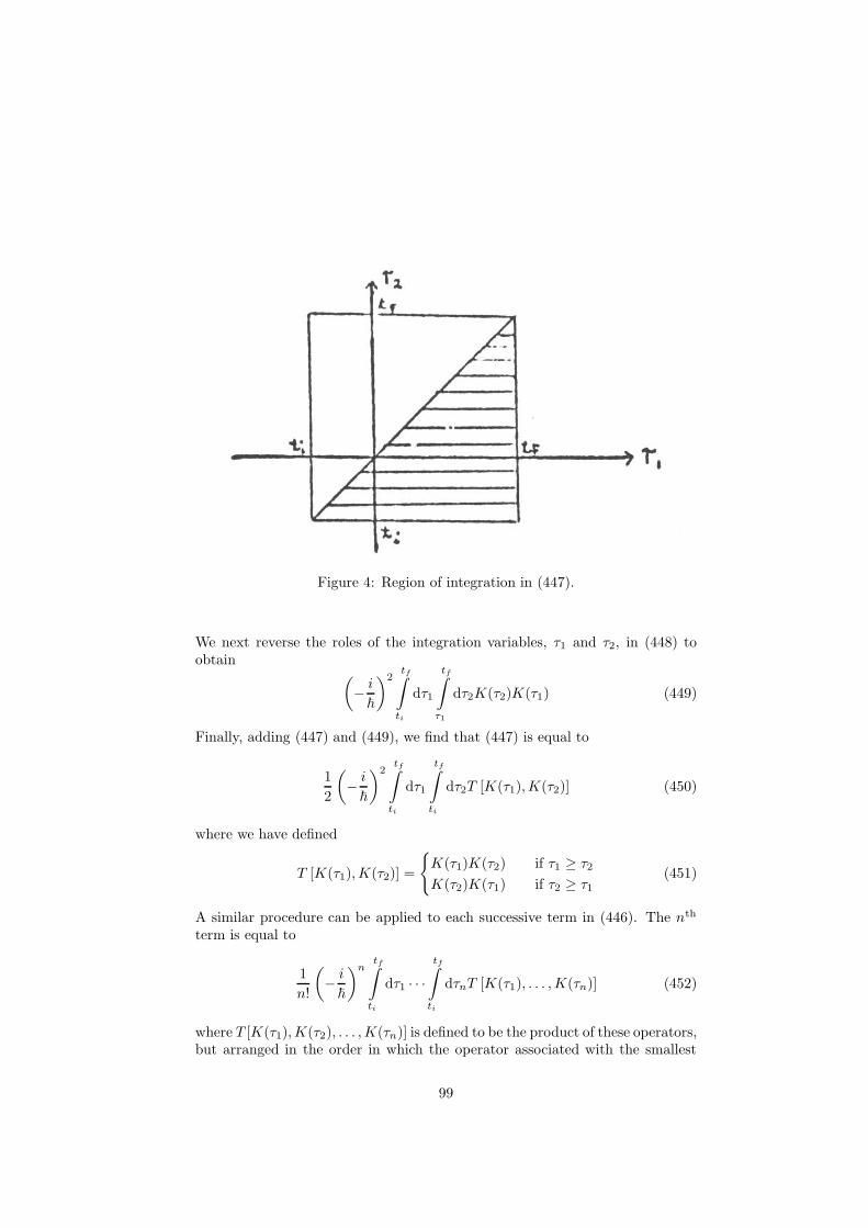
Figure 4: Region of integration in (447).

We next reverse the roles of the integration variables, τ1 and τ2, in (448) toobtain

(− i~

)2tf∫

ti

dτ1

tf∫

τ1

dτ2K(τ2)K(τ1) (449)

Finally, adding (447) and (449), we find that (447) is equal to

1

2

(− i~

)2tf∫

ti

dτ1

tf∫

ti

dτ2T [K(τ1),K(τ2)] (450)

where we have defined

T [K(τ1),K(τ2)] =

{K(τ1)K(τ2) if τ1 ≥ τ2K(τ2)K(τ1) if τ2 ≥ τ1

(451)

A similar procedure can be applied to each successive term in (446). The nth

term is equal to

1

n!

(− i~

)n tf∫

ti

dτ1 · · ·tf∫

ti

dτnT [K(τ1), . . . ,K(τn)] (452)

where T [K(τ1),K(τ2), . . . ,K(τn)] is defined to be the product of these operators,but arranged in the order in which the operator associated with the smallest

99

τm is placed on the right, the operator associated with the next-smallest τmis placed next, etc. This T [K(τ1),K(τ2), . . . ,K(τn)] is called the time-orderedproduct. Thus, our final formal expression for S is

S =

∞∑

n=0

1

n!

(− i~

)n tf∫

ti

dτ1

tf∫

ti

dτ2 · · ·tf∫

ti

dτnT [K(τ1), . . . ,K(τn)] (453)

Note that, if all the K(τ)’s commute, then the time-ordering is irrelevant, and(453) reduces to (439).

To summarize, the only modification of (439) required when the operatorsdo not commute is that the products of operators in the multiple integrals mustbe time-ordered.

Finally, note that if all the K(τ)’s are Hermitian, then, from (436),

d

dt(σ(t), σ(t)) =

(d

dtσ, σ

)+

(σ,

d

dtσ

)

=

(− i~Kσ, σ

)+

(σ,− i

~Kσ

)

=i

~[(Kσ, σ)− (σ,Kσ)] = 0

(454)

Hence, S must be a unitary operator. Unitarity is obvious in (439) — ratherless so in (453).

Our formulae for the S-matrix in field theory will also involve infinite seriesof multiple integrals of time-ordered products of Hermitian operators.

29 The Formula for the S-Matrix

In this section we shall write down the formula for the S-matrix in terms of acertain (as yet unspecified) operator field on Minkowski space. While we shallin no sense “derive” that our expression for S is correct, it will be possible, atleast, to show that the formula is a reasonable guess. We rely heavily on thediscussion in Sect. 28.

Consider Eqn. (453). We wish to write down an analogous formula for Sin quantum field theory. Since, first of all, S is to be an operator on the non-interacting Hilbert space we must take the K’s to be operators on H. Secondly,S should be unitary: we therefore take the K’s to de, Hermitian. By whatshould we replace the interaction variables - the τ ’s in Eqn. (453)? If we thinkof τ in Sect. 28 as representing a “time”, then a natural replacement would beposition x in Minkowski space-time. The integrals in (453) would then extendover all of Minkowski space. (Note: This is the reason why it was convenient, inSect. 28, to obtain an expression in which the integrals extended over the entiret-range from ti to tf .) Thus, we are led to consider the interaction is describedby a certain Hermitian operator field, K(x), which depends on position x in

100

Minkowski space, and acts on H. The S-matrix will then be given by theformula

S =∞∑

n=0

1

n!

(− i~

)n ∫dV1 · · ·

∫dVnT [K(x1), . . . ,K(xn)] (455)

where x1, x2, . . . represent points in Minkowski space, dV1, dV2, . . . the corre-sponding volume elements in Minkowski space, and all integrals are over allof Minkowski space. Note that Eqn. (453) already suffers from one difficulty:the question of the convergence of the infinite series. In writing (455) we haveretained that difficulty, and, in fact , introduced a second one: the question ofthe convergence of the integrals. (The integrals in (453) are all over compactregions.)

In fact, there is a second problem with (455) which was not encountered in(453), namely, the question of what the time-ordering operator T is to meanin (455). In (453), T means that the K(τ) operators are to be placed in theorder of decreasing τ -values. Unfortunately, in the passage from a “time” τ toposition x in Minkowski space-time, the natural ordering is destroyed. There is,however, one case in which points in Minkowski space can be ordered: we agreethat x2 exceeds x1, x2 > x1, if x2−x1 (i.e., the position vector of x2 relative tox1) is future-directed and timelike or null. Hence, for the region of integrationin (455) for which all the x1, . . . , xn can be ordered in this way, T has a well-defined meaning, and hence the integral makes sense. (More explicitly, the τ ’sare totally ordered, while points in (time-oriented) Minkowski space are onlypartially ordered.) Clearly, there is no Poincare-invariant way to “time-order”K(x1) and K(x2) when x2−x1 is spacelike. How, then, are we to give a meaningto (455)? One way of doing this would be through an additional condition onthe K(x). We simply assume that the ordering of K(x1) and K(x2) is irrelevantwhen x2 − x1 is spacelike. That is to say, a natural way of forcing a meaningfor (455) is to assume that the K(x) have the property

[K(x),K(x′)] = 0 for x− x′ spacelike (456)

We include (456) as a requirement on ourK(x). Thus, if x1, x2, . . . , xn are pointsin Minkowski space, we define T [K(x1),K(x2), . . . ,K(xn)] to be the product ofthese operators, placed in an order such that, if xi − xj is timelike or null andfuture-directed, then K(xi) appears before K(xj) in the product. Clearly, therealways exists at least one ordering having this property. Furthermore, (456) im-plies that all such orderings yield the same operator. Thus, T [K(x1), . . . ,K(xn)]is a well-defined operator.

To summarize, the interaction is to be described by giving a Hermitianoperator field K(x) on H which satisfies (456). The S-matrix is to be expressedin terms of K(x) by (455). The formal expression (455) is unsatisfactory insofaras we have investigated the convergence of neither the infinite series nor theintegrals themselves.

The standard textbooks give a more detailed, but, I feel, no more satisfac-tory, argument for (455). One chooses a time-coordinate t in Minkowski space,

101

and writes

H(t) =

∫

t=const.

K(x) (457)

for the “Hamiltonian”. One then imagines a “state vector” in the Hilbert spaceH, σ(t), which depends on the time-coordinate. One writes the “Schrodingerequation”,

−~i

d

dtσ(t) = H(t)σ(t) (458)

The argument of Sect. 28 then yields (455), where T refers to the orderinginduced by the time-coordinate t. Finally Poincare invariance (i.e., the conditionthat S be independent of our original choice of t) requires (456). This argumentassumes, implicitly, that the “states during the interaction” are described by H.We have deviated only slightly from this conventional argument. We isolatedthe simplest and clearest part in Sect. 28, and guessed the rest.

30 Dimensions

With each of the various fields and operators we have introduced, there is associ-ated a corresponding physical dimension. We shall determine these dimensionsin the present section.

Recall that we have set the speed of light equal to one, so length and timehave the same units. (E.g., we measure distance in light-seconds.) We maytherefore take as our fundamental units a mass (m) and a time (t). ThenPlanck’s constant h has dimensions mt. We assign to position vectors in Min-kowski space dimensions t, so the derivative in Minkowski space has dimensionst−1, and the wave operator � dimensions t−2. (Raising, lowering, and con-tracting indices does not affect dimensions.) The quantity µ which appears inthe Klein-Gordon and Dirac equations therefore has dimensions t−1. Positionvectors in momentum space have dimensions t−1. Finally, the volume elementon the mass shell has dimensions t−1 (see (14).)

The rule for determining the dimensions to be associated with a classicalfield is the following: consider an element of the Hilbert space which has normunity, and work back to determine the dimensions of the corresponding field.Consider first the (real or complex) Klein-Gordon case. A unit vector in theHilbert space is represented by a function φ(k) on Mµ which satisfies

1

~

∫

Mµ

φ(k)φ(k) dVµ = 1 (459)

Therefore, φ(k) has dimensions m1/2t3/2. But

φ(x) =

∫φ(k)eikbx

b

dV (460)

and so the Klein-Gordon field has dimensions m1/2t−1/2. For the Dirac case,Eqn. (388) implies that (ξA(k), ηA′(k) has dimensions t1/2. Then (309) and

102

(310) imply that (ξA(k), ηA′(k) has dimensions t3/2. The neutrino fields havethe same dimensions. Finally, for the Maxwell case, (382) implies that Aa(k)has dimensions m1/2t3/2, whence, from (178), Aa(x) has dimensions m1/2t−1/2.(In the Maxwell case, one has a simple independent check on the dimensions.The dimensions above for the vector potential imply that electric and magneticfields have dimensions m1/2t3/2 which agrees, of course, with the dimensionsfrom classical electrodynamics.)

The other quantities whose dimensions are of particular interest are thefield operators. To assign dimensions to these operators, we must decide whatdimensions are to be associated with the test fields. Recall that the role of thetest fields is to smear out the (undefined) operators associated with points ofMinkowski space, e.g.,

φ(f) =

∫f(x)φ(x) dV (461)

Thus, we can think of a test field as a “smearing density.” We therefore takeall test fields to have dimensions t−4. (That is, we require that φ(f) and the(undefined) φ(x) have the same dimensions.) With this convention, the deter-mination of the dimensions of the field operators is straightforward. Considerfirst the Klein-Gordon case. If f(x) is a test field (dimensions t−4), then, from

f(x) =

∫f(k)eikbx

b

dV (462)

f(k) is dimensionless. But a dimensionless element of our Hilbert space, (459),defines a φ(k) with dimensions m1/2t3/2. Therefore, the element of our Hilbertspace associated with this f(k), σ(f), has dimensions m−1/2t−3/2. Thus, thecreation and annihilation operators have dimensions m−1/2t−3/2. But

φ(f) = ~C(σ(f)) + ~A(σ(f)) (463)

(say, for real Klein-Gordon fields), and so the field operators, φ(f), have dimen-

sionsm1/2t1/2. In the Dirac case, the test fields, (fA(x), fA′(x)) have dimensionst−4, whence fA(k) is dimensionless. The corresponding pair of functions on themass shell, (389), therefore has dimensions t−1. Hence, the corresponding ele-ments of our Hilbert space, σ(fA, fA′), have dimensions t−3/2. This, then, isthe dimensions of the creation and annihilation operators. Finally, from (390),the field operators in the Dirac case have dimensions t−3/2. Similarly, in theMaxwell case, fa(x) has dimensions t−4, fa(k) dimensionless, σ(fa) dimensionsm−1/2t−3/2. The creation and annihilation operators therefore have dimen-sions m−1/2t−3/2, and so by (383), the Maxwell field operators have dimensionsm1/2t−1/2.

Note that, in every case, the classical fields and the corresponding fieldoperators have the same dimensions.

103

31 Charge Reversal

An important tool, both for constructing and analyzing interactions, is thediscrete symmetries — charge, parity, and time reversal. We begin with chargereversal.

Let H be a non-interacting Hilbert space, and suppose we are given anoperator S, the S-matrix, on H. What does it mean to say that “the interactiondescribed by S is invariant under charge reversal?” Roughly speaking, thismeans that if we replace any in-state, σ ∈ H, by “the same state, but withall particles replaced by their antiparticles,” then the corresponding out-statesare again “the same, but with particles replaced by antiparticles.” Thus, weare led to try to give a meaning to the notion “the same state (in H), but withparticles replaced by antiparticles.” Let us suppose that this mapping from non-interacting states to non-interacting states is accomplished by come operator Con H, so that Cσ represents the same state as σ, but with particles replacedby antiparticles. Then the statement that the interaction (described by S) isinvariant under charge reversal reduces to the condition

SCσ = CSσ (464)

for any σ ∈ H. In other words, invariance under charge reversal is expressedmathematically by the condition that S and C (both operators on H) commute.

In general, there will be a number of different operators C which could beinterpreted as effecting the replacement of particles by antiparticles. There isno obvious, unambiguous way of translating this physical notion into a math-ematical operator. We shall therefore proceed as follows. We first write downa list of properties which reflect the intuitive idea of “replacing particles byantiparticles, but not otherwise changing the state.” In general, there will hea moderately large class of C’s which satisfy these criteria. Then, for each in-teraction, we look for an operator C which satisfies our criteria and which, inaddition, commutes with the S-matrix. If such a C exists, we say that ourinteraction is invariant under charge-reversal. The point is that any operatorwhich commutes with the S-matrix is valuable. We regard the words “chargereversal” as merely suggesting a particularly fertile area in which such operatorsmight be found. This philosophy is important:

i) there is no natural, a priori charge-reversal operator;

ii) one sets up a class of possible charge-reversal operators, and then selectsfrom this class depending on what the interaction is,

iii) if no operator in this class commutes with the S-matrix, there is littlepoint in considering charge-reversal for that interaction.

(The third point is somewhat over-stated, and will be modified slightly later.)The first condition on C is that it should not mix up particles of different

types. That is to say, C should commute with the total number operators oneach of the Fock spaces which make up H. Therefore, C can be considered

104

as an operator on each of the Fock spaces separately. The assumption that Ccommutes with the total number operators implies, furthermore, that C can bedecomposed into an operator on the one-particle Hilbert space, an operator onthe two-particle Hilbert space, etc. We next assume that the action of C on themany-particle states can be obtained from the action on the one-particle statesas follows. Let H be one of our one-particle Hilbert spaces (e.g., HRKG, HCKG,HM , HD). Then an element of the corresponding Fock space consists of a string

(ξ, ξα, ξαβ , . . .) (465)

of tensors over H . The operator C on the one-particle Hilbert space H can bewritten, in the index notation, as Cαβ : the result of applying Cαβ to an elementξβ of H is written Cαβξ

β . We assume that the action of C on the element (465)of Fock space is

(ξ, Cαβξβ , CαµC

βνξµν , . . .) (466)

This is a quite reasonable assumption: if we know what charge-reversal meanson a one-particle state, we assume that, for a two-particle state, the effect ofcharge reversal is to “apply charge-reversal to each of the particles individually.”

Thus, we are led to distinguish a class of charge-reversal operators on eachof our one-particle Hilbert spaces, HRKG, HM , etc.

It is convenient to introduce some definitions. A mapping T from a Hilbertspace H to itself is said to be antilinear if

T (ασ + τ) = αT (σ) + T (τ) (467)

for any σ, τ ∈ H , α ∈ C. (Alternatively, T could be considered as a linearmapping from H to H .) We shall sometimes refer to an antilinear mapping asan antilinear operator. The word “operator” alone means “linear operator.” Alinear or antilinear operator T is said to be norm-preserving if

‖Tσ‖ = ‖σ‖ (468)

for every σ ∈ H . Eqn. (468) immediately implies that, for any σ, τ ∈ H ,

(Tσ, T τ) = (σ, τ) (469)

or (Tσ, T τ) = (τ, σ) (470)

according as T is linear or antilinear, respectively. As we have remarked, a lin-ear, norm-preserving operator is called unitary. An antilinear, norm-preservingoperator is said to be antiunitary.

Let H be one of the Hilbert spaces HRKG, HCKG, HM , or HD . A linear orantilinear operator C on H will be called a charge-reversal operator if

1. C is norm-preserving.

2. C commutes with all the unitary operators on H which arise from theaction of the restricted Poincare group on H .

105

3. C, applied to a positive- (resp., negative-) frequency element of H , yieldsa negative- (resp., positive-) frequency element.

These conditions are to reflect the intuitive that “the state is changed only inthat particles are replaced by antiparticles.” Conditions 1 and 3 are clearlyreasonable. (The passage from positive-frequency to negative-frequency is thepassage from particles to anti-particles.) Condition 2 ensures that quantitiessuch as the locations and momenta of particles are unchanged under C. Notethat, if C is a charge-reversal operator, and α is a complex number with |α| = 1,then αC is also a charge-reversal operator. (One could, conceivably, impose thefurther condition C2 = 1. We shall not do so.) Note that Condition 1 impliesthat C is also norm-preserving on the non-interacting Hilbert space H.

Before discussing examples of charge-reversal operators, we establish thefollowing result: C must be linear rather than antilinear. Let ra be a constant,unit, future-directed, timelike vector field in Minkowski space. Then the energyoperator associated with ra is

E =i

~raLa (471)

where raLa is the operator which comes from the unitary transformation as-sociated with the Poincare transformation (a translation) generated by ra. Itis essential, in (471), that the i/~ appear explicitly, so that ra is simply thefirst-order difference between a unitary operator and the identity operator. Weassume that C is antiunitary, and obtain a contradiction. For each of our Hilbertspaces, the expectation value of the energy E in any state (and, in particular,in the state C−1σ, for σ ∈ H) is non-negative:

(C−1σ,EC−1σ) ≥ 0 (472)

But, from (470), this implies

(CEC−1σ, σ) ≥ 0 (473)

Write

CEC−1 =

(Ci

~C−1

)(CraLaC

−1) (474)

Condition 2 above implies that C(raLa)C−1. The assumption that C is antiu-nitary implies C(i/~)C−1 = −i/~. Thus, we have

(C−1σ,EC−1σ) = −(Eσ, σ) (475)

But this is a contradiction, for the left side is non-negative and the right sidenon-positive. Therefore, C cannot be anti-linear.

The question of the uniqueness of charge-reversal operators is settled bythe following fact: let O be a bounded operator defined everywhere on H (oneof our four one-particle Hilbert spaces). Suppose that O commutes with theunitary operators which arise from the action of the restricted Poincare group

106

and, furthermore, that O takes positive- (resp., negative-) frequency to positive-(resp., negative-) frequency states. Then O is a multiple of the identity. Iknow of no simple proof. (The statement is essentially an infinite-dimensionalgeneralization of Schur’s Lemma (p. 58).) Now suppose that C and C ′ arecharge-reversal operators. Then C ′C−1 satisfies the conditions above, and hencemust be a multiple of the identity. It follows that C ′ = αC, where α is a complexnumber with |α| = 1. Thus, having found one charge-reversal operator on ourHilbert space H , we have found them all.

We begin with HRKG. In this case, the only positive-frequency or negative-frequency solution is the zero solution. (That is to say, HRKG describes parti-cles which are identical with their antiparticles.) Hence, Condition 3 is empty.Therefore, the identity is a possible charge-reversal operator. We conclude thatthe most general charge-reversal operator on HRKG is αI, with |α| = 1.

For HCKG, one charge-reversal operator is given by

φ(x)→ φ(x) (476)

or, in momentum space, byφ(k)→ φ(−k) (477)

That this operator is unitary rather than antiunitary follows from our complexvector-space structure on HCKG (see Sect. 12). Thus, the most general charge-reversal operator on HCKG is given by

φ(x) → αφ(x) (478)

with |α| = 1.The most general charge-reversal operator on HM is αI, with |α| = 1.The most general charge-reversal operator on HD is

(ξA, ηA′)→ α(ηA, ξA′) (479)

with |α| = 1.

32 Parity and Time Reversal

The basic idea of the remaining two discrete symmetries — parity and timereversal — is essentially the same as that for charge reversal. One is concernedprimarily with finding operators which commute with the S-matrix, and op-erators which can be interpreted as representing parity and time reversal areparticularly good candidates.

We begin with some remarks concerning the Poincare group. Recall that therestricted Poincare group, RP , is a connected, 10-dimensional Lie group. ThisRP is a normal subgroup of another 10-dimensional Lie group, the full Poincaregroup P . However, P is not connected; it has four connected components. Thesecomponents consist of Poincare transformations which reverse neither time norspace orientation (RP), time but not space orientation, space but not time

107

orientation, and both time and space orientation. The quotient group, P/RP,is isomorphic with the group Z2×Z2. (Z2 is the additive group of integers mod2.)

The situation is slightly different for the boson and fermion cases. We beginwith the boson case. Let H be one of the Hilbert spaces HRKG, HCKG, or HM .Then, as we have seen (Sect. 16), H defines a representation of RP . That is tosay, with each P ∈ RP there is associated a unitary operator UP on H , wherethese UP ’s satisfy:

UPUP ′ = UPP ′

Ue = I(480)

The problem of obtaining parity-reversal and time-reversal operators can bestated as follows: we wish to extend this representation from RP to P . Thatis to say, we wish to find, for each P ∈ P , a (unitary or antiunitary) operatorUP , subject to (480) and to the condition that, for P ∈ RP , this representationreduces to the given representation (Sect. 16) of it RP . It is necessary to admitboth unitary and antiunitary operators for, as we shall see shortly, it is otherwiseimpossible to find any extension of our original representation of RP.

There is an important difference between charge reversal on the one hand andparity and time reversal on the other. In the case of charge reversal, one settleseventually on a single unitary charge-reversal operator C. There is, however, noone natural “parity-reversal operator P” or “time-reversal operator T”. Thereis, instead, a 10-dimensional manifold’s worth of such operators, namely, theoperators associated with the appropriate component of the Poincare group.

Suppose now that we have a representation of P as described above. LetP and Q be in the same component of P , so PQ ∈ RP . Now UPUQ = UPQ.But, since PQ ∈ RP , UPQ is unitary rather than antiunitary. We concludethat either both UP and UQ are unitary, or else both are antiunitary. (Theproduct of two unitary operators, or two antiunitary operators, is unitary; theproduct of a unitary and an antiunitary operator is antiunitary.) We concludethat all the operators associated with the Poincare transformations in a givencomponent of P are the same (all unitary or all antiunitary.)

In fact, it follows from an argument similar to that used for charge-reversalthat UP is antiunitary if and only if the Poincare transformation P reversestime. From the remarks above, it suffices to show that, for some P whichreverses parity but not time, UP is unitary, and that, for some P which reversestime but not parity, UP is antiunitary. Let ra be a constant, unit, future-directedtimelike vector field, and consider the energy operator E given by (471). Allexpectation values of E are non-negative. Fix an origin O, and let ta be a unit,future-directed timelike vector at O. Let P denote the Poincare transformationwhich sends

xa → xa + 2ta(xbtb) (481)

where xa is the position vector relative to O. Evidently, this P reverses timeorientation but not space orientation. From the commutativity properties of

108

the Poincare group,

U−1P EUP =

(U−1P

i

~UP

)r′aLa (482)

wherer′a

= ra + 2ta(rbtb) (483)

Since r′a is a past-directed timelike vector, the positivity of E implies, evidently,that UP must be antiunitary. Similarly, let Q be the Poincare transformation

xa → −xa − 2ta(xbtb) (484)

So Q reverses spatial orientation but not time orientation. Then

U−1Q EUQ =

(U−1Q

i

~UQ

)r′aLa (485)

wherer′a

= −ra − 2ta(rbtb) (486)

Clearly, in this case r′a is a future-directed timelike vector, hence UQ must beunitary.

We next consider uniqueness. Let UP and U ′P be two extensions of our repre-sentation of RP , so UP = U ′P for P ∈ RP . Let Q be a Poincare transformationwhich reverses, say, temporal orientation but not spatial orientation. Considerthe unitary operator

A = U ′QU−1Q (487)

We first how that this A depends only on the component of P in which Q lies.Let W be another Poincare transformation which lies in the same componentof P as Q. Then W = QR for some R ∈ RP . Hence,

U ′WU−1W = U ′QRU

−1QR = (U ′QU

′R)(U−1

R U−1Q ) = U ′QU

−1Q (488)

where we have used the fact that UR = U ′R. We next show that, for P ∈ RP ,UP commutes with A. Indeed, since PQ = QV for some V ∈ RP , we have

UPAU−1P = UPU

′QU−1Q U−1

P = U ′PQU−1PQ

= U ′QV U−1QV = (U ′QUV )(U−1

V U−1Q ) = U ′QU

−1Q = A (489)

These properties do not yet suffice, however, to show that A is a multiple of theidentity (see p. 106). We must impose an additional condition which ensuresthat A does not mix up particles and antiparticles. However, it is reasonable,on physical grounds, to make the following additional assumption: UP reversesthe roles of particles and antiparticles if and only if P reverses time directions.Under this assumption, A must be a multiple of the identity, whence UQ = αU ′Q,where α is some complex number (the same for every on Poincare transformationin the same component as Q). However, since QQ ∈ RP , we have

U ′QU′Q = U ′QQ = UQQ = UQUQ (490)

109

whence α = ±1.To summarize, we are interested in extending a given representation from

RP to P in such a way that UP reverses the role of particles and antiparticleswhen and only when P reverses temporal orientation. Every such extension hasthe property that UP is antiunitary when and only when P reverses temporalorientation. The extension of the representation is unique except for the follow-ing possibilities: affix a minus sign to UP whenever P reverses spatial parity,affix a minus sign to UP whenever reverses temporal orientation, or affix a minussign to UP whenever P reverses spatial or temporal orientation, but not both.Thus, from one extension of the representation, it is easy to write down themall.

Finally, we write down a representation of P for each of our Hilbert spacesHRKG, HCKG, and HM . Let P be a Poincare transformation, and write Pxfor the point of Minkowski space to which P sends the point x. For the realand complex Klein-Gordon cases, the action of UP on an element φ(x) of ourHilbert space is as follows:

φ(x) → φ(Px) (491)

This action clearly defines a representation of P . For the Maxwell case, notethat P is a smooth mapping from Minkowski space to Minkowski space, andhence P sends any vector field on Minkowski space to another vector field. Thisaction defines UP on HM . For example, the two Poincare transformations (481)and (484) have the following actions on the vector potential Aa(x):

Aa(x)→ Aa(Px) + 2ta(tbAb(Px))

Aa(x)→ −Aa(Qx)− 2ta(tbAb(Qx))(492)

The situation with regard to HD differs in some important respects from thatabove. The fundamental difference is that HD does not define a representationof RP . Instead, the operative group is what is usually called “inhomogeneousSL(2,C)”: the (double) covering group of RP . (SL(2,C) is the (double) cov-ering group of the restricted Lorentz group.) We shall denote this connected,10-dimensional Lie group by RS . If RS is to replace RP , what group shouldreplace P? One could, in fact, introduce such a group, and attempt to extendto it our representation of RS . It is simpler, however, to proceed in a slightlydifferent way.

Let P ∈ RP . Associated with P there are precisely two elements of RS .The corresponding pair of unitary operators on HD differ only in sign. Thus,we can regard HD as a double-valued representation of RP : with each P ∈ RP ,there is associated two unitary operators on HD, these operators differing onlyin sign. These operators satisfy (480), modulo sign. The question in the fermioncase is therefore the following: Can this double-valued representation of RP beextended to a double-valued representation of P? The argument given earliershows that the operators associated with P ∈ P are antiunitary if and only if Preverses time-orientation. The uniqueness situation is essentially the same, bythe same argument.

110

There remains, therefore, only the task of specifying what the operators arefor P /∈ RP . Since the (double-valued) action of RP on HD is known, we needonly specify UP for one time-reversing P and one parity-reversing P . The actionis as follows. For the Poincare transformation (481),

(ξA(x), ηA′ (x))→ ± i√2

(tAA′ηA′(Px), tAA′ξ

A(Px)) (493)

and for the Poincare transformation (484),

(ξA(x), ηA′(x)) → ± 1√2

(tAA′ηA′(Qx), tAA′ξ

A(Qx)) (494)

33 Extending Operators to Tensor Products

and Direct Sums

We have now introduced a large number of operators — some on the one-particleHilbert spaces and some of the Fock spacs. In order that such operators can bediscussed relative to the S-matrix, however, their action must be defined on thenon-interacting Hilbert space H. Since H arises from two constructions — thetensor product and direct sum of Hilbert spaces — we are led to the problemof extending the action of operators through these two constructions.

We begin with the direct sum. Let H1, H2, . . . be a sequence of Hilbertspaces. Then the direct sum of this sequence, H = H1 ⊕H2 ⊕H3 ⊕ . . . is theHilbert space consisting of sequences

σ = (σ1, σ2, σ3, . . .) (495)

with σi ∈ Hi for which the sum

‖σ‖2 = ‖σ1‖2 + ‖σ2‖2 + · · · (496)

which defines the norm, converges. Now let O1, O2, . . . be a sequence of operators(Oi onHi) which are either all linear or all antilinear. We then define an operatorO on H as follows:

Oσ = (O1σ1, O2σ2, O3σ3, . . .) (497)

Clearly, O is linear (resp., antilinear) provided the Oi are linear (resp., antilin-ear.) Note, furthermore, that if all the Oi are norm-preserving, so is O; if allthe Oi are Hermitian, so is O; if all the Oi are projection operators, so is O. Ofcourse, not every operator on H can be expressed in the form (497).

The tensor product is next. Let Hα, Hβ, . . . , Hδ be a finite sequence ofHilbert spaces. Then the tensor product of this sequence, H = Hα⊗Hβ⊗· · ·⊗Hδ is the Hilbert space obtained as the completion of the inner-product spaceconsisting of all formal expressions of the form:

ξαβ···δ = σατβ · · ·µδ + · · ·+ λαρβ · · · νδ (498)

111

(The index indicates the Hilbert space to which a vector belongs.) Now letOα′α, O

β′β , . . . , O

δ′δ be a sequence of linear operators on Hα, Hβ , . . . , Hδ , re-

spectively. We then can define an operator O on H by:

O(ξαβ···δ) = (Oα′ασ

α)(Oβ′βτ

β) · · · (Oδ′ δµδ) + · · ·+ (Oα

′αλ

α)(Oβ′βρ

β) · · · (Oδ′ δνδ) (499)

If all the O’s are unitary, so is O; if all the O’s are Hermitian, so is O; if all theO’s are projection operators, so is O. Now suppose that the given O-operatorsare antilinear rather than linear. We thus have linear mappings from Hα toHα, from Hβ to Hβ , etc. Thus, in the index notation, the O’s would be written

Oα′α, Oβ

′β , . . . , Oδ′δ. In this case, we define the corresponding operator O on

H by

O(ξαβ···δ) = (Oα′ασα)(Oβ

′β τβ) · · · (Oδ′δµδ) + · · ·+ (Oα

′αλα)(Oβ′β ρβ) · · · (Oδ′δνδ) (500)

If the O’s are anti-unitary, so is O.We next consider the application of these constructions to obtaining opera-

tors on H. Recall that the non-interacting Hilbert space H is the tensor productof certain Fock spaces based on one-particle Hilbert spaces, e.g.,

H = F(HD)⊗F(HM )⊗F(HCKG) (501)

where F denotes the operation of taking the (symmetric or antisymmetric, asappropriate) Fock space.

Consider first the unitary or antiunitary operators UP (P ∈ P) which arisefrom the Poincare group. These operators are defined originally on the one-particle Hilbert spaces. Their action is first extended to the many-particleHilbert spaces via (499) or (500), and then to the Fock spaces via (497). Fi-nally, these operators are defined on H via (499) or (500). Thus, we obtaina representation of the Poincare group P on H. For P ∈ P , we write thecorresponding operator on H as UP . (No confusion will result from this du-plicity of notation.) Note that all the operators UP on H are norm-preserving,and that UP is antilinear if and only if P reverses time orientation, linear oth-erwise. The energy, momentum, and angular momentum operators on H areobtained by considering the UP ’s which differ infinitesimally from the identity(see Eqn. (222).) Similarly, the charge-reversal operator C is defined, first, onthe one-particle Hilbert spaces, and then extended successively to the many-particle spaces, to the Fock spaces, and finally to H. The resulting operator onH is again denoted by C.

Another operator of interest is the total charge operator, Q. On our realHilbert spaces (which represent neutral particles), HRKG and HM , Q = 0. Onthe complex Hilbert spaces, HCKG and HD, Q takes one of the two forms

Q = eP− − eP+ (502)

112

Q = eP+ − eP− (503)

where P+ and P− are the projection operators onto positive-frequency andnegative-frequency parts, respectively. The choice between (502) or (503) isbased essentially on convention. One uses (502) when the “particles” (positive-frequency solutions) have negative charge, and (503) when they have positivecharge. (For example, one could perfectly well dictate that the positron is the“particle”, and the electron the antiparticle. It is conventional, however, tomake the assignments the other way. This choice his no physical consequences.)Note that, in every case, Q is Hermitian. We extend Q from the one-particle tothe many-particle Hilbert spaces via (499), to the Fock spaces via (497), and toH via (499). The result is a Hermitian charge operator, Q, on H.

Finally, we consider the creation, annihilation, and field operators. Theseoperators, in distinction to the others defined above, are first defined on the Fockspaces rather on the one-particle Hilbert spaces. Suppose, for example, that His given by (501), and we are considering the field operator φ(f) on F(HCKG).Now consider the following triple of operators: I (the identity) on F(HD), I onF(HM ), and φ(f) on F(HCKG). This triple defines, via the construction (499),an operator on H. In this way, the creation, annihilation, and field operatorsare extended from a single Fock space to H. The resulting operators on H will,as usual, be denoted by the same symbols as the corresponding operators onthe single Fock spaces.

All of the commutators and other relations between these various operatorson H are simple to evaluate. We give a few examples. The operators associatedwith the Poincare group satisfy, of course,

UPUP ′ = UPP ′ (504)

The UP ’s leave invariant the charge of an element of H if P does not reversethe orientation, and reverse that sign if P does reverse time orientation. Hence,we have

UPQU−1P = ±Q (505)

with the plus sign if P does not reverse time orientation, the minus sign other-wise. Of course, charge-reversal reverses the sign of charge:

CQC−1 = −Q (506)

The commutators between the field operators (and the creation and annihilationoperators) within one Fock space are the same for H as for the original Fockspace. That is, for example, we have

[φ(f), φ∗(g)

]=~2iD(f, g)I (507)

on H. Similarly, the adjoint relations between these operators are unchanged inthe passage to H. Field operators (as well as creation and annihilation opera-tors) which act on different Fock spaces commute. For example,

[φ(f), A(fa)

]= 0 (508)

113

Finally, we consider the relationship between the field operators and C, Q, andUP . Once again, everything is straightforward, so a single example will suffice.Consider HCKG, so

φ(f) = ~C(σ−(f)) + ~A(σ+(f))

φ∗(f) = ~A(σ−(f)) + ~C(σ+(f))(509)

Let P be a restricted Poincare transformation. Then, from (497), (499), (100),and (101),

UPφ(f)U−1P = ~C(UPσ

−(f) + ~A(UPσ+(f)) (510)

Similarly, if C is a particle-reversal operator, then

Cφ(f)C−1 = ~C(Cσ−(f)) + ~A(Cσ+(f))

= ~C(σ+(f)) + ~A(σ−(f)) = φ∗(f)(511)

For the charge operator Q, we note that φ(f) creates an antiparticle (say, withpositive charge) and annihilates a particle. Hence, the total change in the chargeeffected by φ(f) is just −e times the norm of σ−(f) plus −e times the norm ofσ+(f). Thus,

[Q,φ(f)] = −e(‖σ+(f)‖+ ‖σ−(f)‖

)I (512)

Clearly, the list of operators in this subject is almost infinite. Roughly speaking,any two operators in this list have a relationship which is simple, straightforwardto derive, and easy to interpret physically.

34 Electromagnetic Interactions

In Sect. 29 (see Eqn. (455)) we wrote down an expression for the S-matrix interms of an (unknown) operator field K(x) on Minkowski space. Of course,this formula gives practically no information about the scattering unless oneknows K(x). One imagines that the actual K(x) which describes physical pro-cesses in the real world can be written as the sum a certain number of terms(e.g., the electron-photon interaction, the nucleon-photon interaction, the π-meson-photon interaction (electromagnetic interactions), the π-meson-nucleoninteraction (strong interactions), the electron-neutrino interaction, the π-meson-neutrino interaction (weak interactions), etc.) There are at least some exper-imental situations in which one single term dominates all the others. One at-tempts to obtain an expression for this term using physical arguments and trialand error. That is to say, one makes a reasonable guess for the term in K(x),and compares the theoretical consequences of that guess (via (455)) with ex-periment. The hope is that one can, in this way, isolate and study each term,and then, by adding the well-established terms, obtain a reasonable approxima-tion to the “actual” K(x) which is operative in Nature. We shall here merelyillustrate the general idea by writing down and discussing a few of the K(x)’sassociated with the interaction of charged particles with the electromagneticfield.

114

We begin with the simplest case: the interaction of a complex Klein-Gordonfield with the Maxwell field, e.g., the interaction of π±-mesons with photons. Inthis case, we would take for our non-interacting Hilbert space

H = F(HCKG)⊗F(HM ) (513)

What should we choose for the operator field K(x) on H? In this case, we havean important physical clue: we know what the classical “interaction energydensity” is between a classical Klein-Gordon field and a classical Maxwell field,namely

K(x) =ie

2~(φ(x)∇aφ(x)− φ(x)∇aφ(x)

)Aa(x) (514)

(Note that it is only an integral of (514) which has meaning, for we have the free-dom to add a gradient to the vector potential. Appropriate integrals are gauge-invariant, however, because the first integral is, as we have seen, divergence-free.) In (514), e is a constant. Using the discussion of Sect. 30, and the factthat K(x) has dimensions of energy density (mt−3), we see that the couplingconstant e has dimensions m1/2t1/2, whence e2/~ is dimensionless. In order toobtain eventual agreement with experiment, it will, of course, be necessary toset this constant to 1/137.

While (514) is a perfectly nice scalar field (on Minkowski space) constructedout of a complex Klein-Gordon field and a Maxwell field, it is, unfortunately, justthat — a scalar field rather than an operator field. The expression (514) is justnot the right sort of mathematical object to be K(x). Now comes the “transitionfrom classical to quantum theory.” Roughly speaking, what we propose to dois to replace the classical fields in K(x) (Eqn. (514)) by the corresponding fieldoperators to obtain K(x). Unfortunately, this replacement is not so simple andunambiguous as it may appear at first sight.

By what operator should we replace φ(x)? Our Klein-Gordon field operator,φ(f), depends on test fields in Minkowski space, and not on points of Minkowskispace. What one would like to do is define an operator field φ(x) by

φ(x) = limf→δx

phi(f) (515)

where δx denotes a δ-function located at the point x. But will the limit in (515)exist? The answer, as we have seen earlier, is no. We could still regard φ(x)as an operator-valued distribution (i.e., a linear mapping from test functionsto operators on H — that, after all, is what φ(f) is), but such an attitudeagain leads to difficulties. Eqn. (514) will require us to take products of suchoperator-valued distributions, but the ability to take products is precisely whatis lost in the transition from functions to distributions. That is to say, productsof distributions are not in general well-defined. (This is a genuine and seriousproblem — not to be confused, for example with the standard complaints aboutuse of the Dirac δ-function.) In short, we are stuck. There is no meaning whichcan be given to (515) which would be appropriate for replacement in (514).

We adopt the following attitude. We leave the problem of the nonexistenceof limits such as (515) unresolved for the time being. We permit ourselves to

115

manipulate such quantities formally, as though the question of the limits hadnever arisen. This marks the third (and, mercifully, the last) of the mathe-matical problems associated with this formalism. For emphasis, we list theseproblems again:

1. The question of the convergence of the infinite sun of operators in (455).

2. The question of the convergence of the integrals (over all of Minkowskispace) of operators in (455).

3. The nonexistence of the “δ-function limits” of field operators used in ob-taining K(x).

The situation will look less gloomy shortly. (I find it hard to believe that the“ultimate”, mathematically acceptable, quantum field theory will result from abrute-force attack on these problems.)

We now have φ(x) to replace φ(x). Naturally, we replace the classical

complex-conjugate field, φ(x), by the adjoint operator, φ∗(x). What aboutthe derivative terms? Let pa be a vector at the point x, and extend pa to aconstant vector field on Minkowski space. We then define

pa∇aφ(x) = − limf→δx

φ(pa∇af) (516)

(See Eqn. (145).) Similar remarks concerning non-existence of limits apply.We must next select an operator to replace the vector potential, Aa(x), in

(514). Ideally, one would like to define ulAa(x) by

paAa(x) = limf→δx

A(paf) (517)

where pa is a constant vector field, and A( ) is the field operator (Sect. 14) forthe vector potential. Unfortunately, this won’t work, for A(f a) is only definedfor test fields fa which can be written as the sum of a divergence-free field anda gradient; paf cannot be written in this form in general. The simplest way ofovercoming this difficulty is as follows. First note that the commutator of thevector potential operators ((385) and (386)) is well-defined whether or not thetest fields, fa and ga, can be written as the sum of a divergence-free field anda gradient. In fact, it is only these commutators which will enter the S-matrix.Hence, we can work with vector potential operators, Aa(x), and use for thecommutators (385).

We now have an operator equivalent for each term in (514). We must nowface the next problem: in what order should the operators be placed? This diffi-culty does not arise, of course, in the classical theory, because the classical fieldsmay be placed in any order. We consider the most general linear combination:

K(x) =ie

2~(aφ∇aφ∗ + b(∇aφ∗)φ+ cφ∗∇aφ+ d(∇aφ)φ∗

)Aa (518)

where a, b, c, and d are real numbers. Taking the Hermitian conjugate of (518),

K(x) = − ie2~(a(∇aφ)φ∗ + bφ∗∇aφ+ c(∇aφ∗)φ+ dφ(∇aφ∗)

)Aa (519)

116

We see that the Hermiticity of (518) requires

a = −d b = −c (520)

Further information about the coefficients is obtained from the experimentalfact that electromagnetic interactions are invariant under charge reversal. From(518):

CK(x)C−1 =ie

2~(aφ∗∇aφ+ b(∇aφ)φ∗ + cφ∇aφ∗ + d(∇aφ∗)φ

)Aa (521)

Thus, invariance under charge reversal requires one of the following two alter-natives:

a = c b = d CAaC−1 = Aa (522)

a = −c b = −d CAaC−1 = −Aa (523)

We choose (523) for two reasons: (i) it is more reasonable on physical groundsto have the vector potential reverse sign under charge reversal (for classicalelectromagnetic fields reverse sign when the signs of all charges are reversed),and (ii) with this choice, K(x) reduces, in the classical limit, to the classicalexpression (514). Thus, we arrive at the interaction:

K(x) =ie

4~(φ∇aφ∗ + (∇aφ∗)φ− φ∗∇aφ− (∇aφ)φ∗

)Aa (524)

Eqn. (524) describes an interaction which is invariant under charge reversal.Note, furthermore, that if P is any Poincare transformation, then

UPK(x)U−1P = K(Px) (525)

Since K(x) is integrated over all of Minkowski space (Eqn. (455)), the finalS-matrix will commute with each UP . Thus, our interaction conserves thequantities associated with the infinitesimal generators of energy, momentum,and angular momentum. The interaction is also invariant under parity andtime reversal. Note, furthermore, that we have

[K(x),K(y)] = 0 (526)

for x − y spacelike, for when x − y is spacelike, any two operators in (524)commute with each other. Finally, the total charge operator, Q, commuteswith K(x), for Aa(x) commutes with Q, φ(x) decreases the total charge by 2e,while φ∗(x) increases it by 2e.

To summarize, (524) is an interaction which is invariant under parity, time,and charge reversal, and conserves charge, energy, momentum, and angularmomentum.

As a second example, we discuss the interaction of photons with electronsand positrons. As before, we begin with the classic interaction energy density:

K(x) = e(ξAξA

′+ ηA

′ηA)AAA′ (527)

117

The classical Dirac fields are to be replaced by the following operators:

pAξA(x) = lim

f→δx

1

2

[ψ(fpA, f pA′)− iψ(ifpA,−if pA′)

]

pA′ηA′

(x) = limf→δx

1

2

[ψ(fpA, f pA′) + iψ(ifpA,−if pA′)

] (528)

where pA is a constant spinor field. Note that e in (527) again has dimensionsm1/2t1/2. The classical complex-conjugate fields, ξA

′and ηA, are to be replaced

by the Hermitian conjugates, ξ∗A′and η∗

A, respectively. In this case, the problem

of factor ordering is not resolved by the requirement that K(x) be Hermitian:this condition is satisfied for any factor ordering. However, this electromagneticinteraction should be invariant under charge reversal. We have

CξAC−1 = η∗A

CηA′C−1 = ξ∗

A′

(529)

What should we adopt for the behavior of the vector potential operator, Aa(x),under charge reversal? We have already decided, for the meson-photon interac-tion, to use

CAaC−1 = −Aa (530)

It is an important point that we must choose the same behavior for the presentinteraction. The reason is that, for the “actual” interaction which Nature obeys,K(x) will be the sum of the various interactions. If we use a different charge-reversal operator for each term which appears in this sum, then we will have nooperator which commutes with the total K(x). In other words, the behavior ofeach type of particle under the various reversals must be fixed once and for all.One has, of course, freedom to choose that behavior, and this choice is basedon obtaining operators which commute with as many terms in the “final” K(x)possible. Thus, using (529) and (530), we are led to adopt the expression

K(x) =1

2e(ξAξ∗A

′ − ξ∗A′ξA + ηA′η∗A − η∗AηA′

)AAA′ (531)

for the interaction.Note that (530) is Hermitian, and that the resulting S-matrix commutes

with the unitary operators which arise from the Poincare group. Thus, (530)conserves energy, momentum, and angular momentum. By the same argumentas before, K(x) commutes with the total charge operator Q. Finally, we notethat, if x− y is spacelike,

[K(x),K(y)] = 0 (532)

This arises from the following facts: when x − y is spacelike, any two bosonoperators commute, while any two fermion operators anticommute. But K(x)contains an even number of fermion operators. Since reversing the order oftwo boson operators gives a plus sign, and reversing the order of two fermion

118

operators gives a minus sign, the total number of minus signs will be even, andso we have (532).

Clearly a vast number of conceivable interactions could be written downusing the pattern illustrated above. One first writes down a real scalar fieldconstructed from the classical fields. One then replaces the classical fields bythe corresponding operators. The factors must be ordered so that the resultingoperator is Hermitian, and satisfies (532). Beyond that, the choice of factorordering must be based on physical or aesthetic considerations, experiment, etc.We have merely discussed two possible interactions here in order to illustratethe method. (In fact, these are the two simplest, for one can rely heavily onclassical theory as a guide.)

35 Transition Amplitudes

Suppose now that we have selected a particular K(x), and wish to work outits experimental consequences, using (455). The straightforward procedure —substituting K(x) into (455), and attempting to carry out the integrals and sum— turns out to be too difficult to carry out in practice. Instead, one adoptsa more indirect approach — which leads ultimately to the Feynman rules. Weshall not attempt to derive the Feynman rules, or even discuss the large volumeof technical apparatus which has been developed to deal with (455). Instead,we merely indicate the general idea of the method.

Suppose first that we were able, in some way, to obtain the value of thecomplex number

(τ, Sσ) (533)

for any two states σ, τ ∈ H. (The expression (533) is called the transitionamplitude between the state σ and the state τ .) This information is, of course,completely equivalent to a knowledge of the S-matrix. In fact, it suffices to know(533) only for σ’s and τ ’s drawn from a certain subspace of H, provided thissubspace is dense in H. Let σ0 denote the vacuum state in H and C1, C2, . . . , Cnany finite sequence of creation operators on H. (One Ci might create a photon,another an electron, others mesons, etc.) We consider the state (element of H)

C1C2 · · ·Cnσ0 (534)

Clearly, the collection of all finite linear combinations of states of the form (534)is dense in H. Hence, it suffices to evaluate

(C1 · · ·Cnσ0, SC′1 · · ·C ′mσ0) = (C1 · · ·Cnσ0, C

′1 · · ·C ′mσ0)

+

(− i~

)∫dV1(C1 · · ·Cnσ0,K(x1)C ′1 · · ·C ′mσ0)

+1

2!

(− i~

)2 ∫dV1

∫dV2(C1 · · ·Cnσ0, T [K(x1),K(x2)]C ′1 · · ·C ′mσ0)

+ · · · (535)

119

for any C1, . . . , Cn, C′1, . . . , C

′m. One now attempts to evaluate the various terms

in the sum (535) individually. The first term is celled the 0th-order interaction.It clearly vanishes unless n = m, and the C’s and C ′’s create the same numberof photons, the same number of electrons, etc. The second term is called thefirst-order interaction, etc. These orders correspond to the various orders of theFeynman diagrams.

The next step is based on the following observation. The operator K(x) isexpressed in terms of the field operators, and can, therefore, be written in termsof creation and annihilation operators. Thus, each inner product in (535) isequal to the vacuum expectation value of some product of creation and annihi-lation operators. But we have seen (p. 89) that such expectation values can bereduced to products of the propagators. (One pushes the annihilation operatorsto the the right, using the commutators, until they reach σ0, and there givezero.) Thus, each term in (535) can be written as an integral of a product of op-erators. The Feynman rules represent a technique for writing out such integralsdirectly without going through the algebra (p. 89). Since K(x) was expressed interms of the “unsmeared” field operators, the propagators will be distributions.Thus, the evaluation of the S-matrix reduces to integrating certain products ofdistributions over Minkowski space. Of course, the integrals diverge. These arethe divergences.

We illustrate these remarks with one example. Consider the second-orderinteraction with K(x) given by (531). Now, K(x) contains two lepton operatorsand one photon operator. Thus, the transition probability will vanish (in thesecond order) unless the number of outgoing leptons differs by no more thanfour from the number of ingoing leptons, and the number of outgoing photonsdiffers by no more than two from the number of ingoing photons. Clearly,the higher the order of the interaction, the more possibilities for creating andannihilating particles. Because of the smallness of the coupling constant in thiselectromagnetic interaction, e2/~ = 1/137, many experiments are adequatelydescribed by the first few orders.

“Would it not be better to get something done, even though onemight not quite understand what?”

– J. L. Synge

120