Special random variables

Chapter 5 Some discrete or continuous

probability distributions

Some special random variables

Bernoulli Binomial Poisson Hypergeometric Uniform Normal and its derivatives

Chi-square T-distribution F-distribution

Exponential Gamma

Bernoulli random variable

A random variable X is said to be a Bernoulli random variable if its probability mass function is given as the following: P{X=0}=1-p, P{X=1}=p; (you may assume X=1 whe

n the experimental outcome is successful and X=0 when it is failed.)

E[X]=1×P{X=1}+0×P{X=0}=p Var[X]=E[X2]-E[X]2 =p(1-p)

Binomial random variable Suppose there are n independent Bernoulli trials,

each of which results in a “success” with the probability p.

If X represents the number of successes that occur in the n trials, then X is said to be a binomial random variable with parameters (n,p). P{X=i}= n!/[(n-i)! ×i!] × pn(1-p)(n-i) , i=0, 1, 2,…n

niC

1)]1([)1()()(00

nn

i

inini

n

i

ppppCiXp

The expectation of binomial random variable

The Binomial random X is composed of n independent Bernoulli trials

∴X=Σ1~nxi, xi =1 when the ith trial is a success or xi =0 otherwise

E[X]=Σ1~nE[xi]=n×p Var[X]=Σ1~nVar[xi]=np(1-p)

Patterns of binomial distribution If p=0.5, then X will distribute

symmetrically If p>0.5, then X will be a left-

skewed distribution If p<0.5, then X will be a right-

skewed distribution If n∞, then X will distribute as a

symmetric bell/normal pattern

Poisson random variable The random variable X is a Poisson

distribution if its prob. mass function is given by

1!

)(

,...2,1,0,!

][

0

00

eeei

eiXP

ii

eiXP

i

i

i

i

(By the Taylor series)

Expectation and variance of Poisson distribution

By using the moment generating function

)}1(exp{

)!/)()!/(][)(00

te

i

it

i

ititX

eee

ieeieeeEt

t

222'"

'

2"

'

)0()0(][

,)0(][

)}1(exp{)}1(exp{)()(

)};1(exp{)(

XVar

XE

eeeet

eettttt

tt

Poisson vs. Binomial A binomial distribution, (n,p), a Poisson with me

anλ=np, when n is large and p is small. In other words, if the successful probability of trial

is very small, then the accumulative many trials distribute as a Poisson. The probability of one person living over 100 years of ag

e is 0.01, then the mean number of over-100-year-old persons 10 may occur within 1000 elders.

λ means the average occurrence among a large number of experiments, in contrast to, p means the occurring chance of every trial

Comparisons

A binomial random variable with p near to 0.5A Poisson random variable approximates to a binomial distribution when n becomes large.

Hypergeometric random variable

There are N+M objects, of which N are desirable and the other M are defective. A sample size n is randomly chosen from N+M without replacements.

Let X be the number of desirable within n chosen objects. Its probability mass function as the following.

),min(,...2,1,0,][ nNiC

CCiXP

MNn

Min

Ni

We said X is a hypergeometric distribution with parameters (N,M,n)

Expectation & variance of hypergeometric distribution

n

1i

n

ji1

n

1i

n

1i

1

),(2)()(

)()1(][E[X]

n size of sample in the outcome desired ofnumber theis X ,

otherwise0,

desirable isselection ith theif 1,

njii

ii

n

ii

i

XXCovXVarXVar

MNnNXPXE

XX

X

Expectation & variance of hypergeometric distribution (cont.)

1

11p)-np(1Var(X) np,E(X) then M),N/(Nplet if

)1

11(

)()1()(2

)()(

)1()(

jifor ,)()1)((

)1(][][][),(

1

1)1,1()1(][

2222

2

2

MN

n

MN

n

MN

nMN

MNMN

NMC

MN

nMNXVar

MNMN

NM

MN

N

MNMN

NNXEXEXXEXXCov

MN

N

MN

NXXPXXPXXE

n

jijiji

jijiji

Moreover, if N+M increases to ∞, then Var(X) converges to np(1-p), which is the variance of a binomial random variable with parameters (n,p).

hypergeometric vs. binomial Let X, and Y be independent binomial ran

dom variables having respective parameters (n,p) and (m,p). The conditional p.m.f. of X given that X+Y=k is a hypergeometric distribution with parameters (n,m,k).

The Uniform random variable

A random variable X is said to be uniformly distributed over the interval [α,β] if its p.d.f. is given by

1)(1

otherwise ,0

Xα if ,1

)(

dx

xf

Pattern of uniform distribution

Expectation and variance of uniform distribution

E[X]=∫α~β x[1/(β-α)]dx=(α+β)/2 Var(X)=E[X2]-E[X]2

=(β-α)2/12 P.161, Example 5.4b

Normal random variable A continuous r.v X has a normal distribution

with parameter μ and σ2 if its probability density function is given by:

We write X~N(μ,σ2)

By using the M.G.F., we obtain E[X]=ψ’(0)=μ, and Var[X]=ψ”(0)-ψ’(0)2=σ2

Standard normal distribution

adzea

a z - ,2

1)( 2/2

The Cumulative Distribution function of Z

symmetry)(by ),(1}{}{)(

)()(

}{}{

)(}{}{

aaZPaZPa

ab

bXaPbXaP

bbXPbXP

Percentiles of the normal distribution

Suppose that a test score distributes as a normal distribution with mean 500 and standard deviation of 100. What is the 75th percentile score of this test?

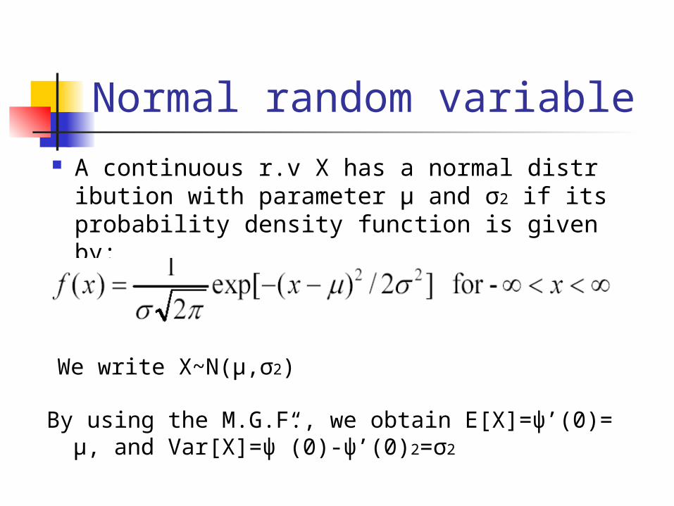
Characteristics of Normal distribution

P{∣X-μ∣<σ}=ψ(-1<X-μ/σ<1)=ψ(-1<Z<1)= ψ(1)-ψ(-1)=2ψ(1) -1=2× 0.8413-1P{∣X-μ∣<2σ}=ψ(-2<X-μ/σ<2)=ψ(-2<Z<2)= ψ(2)-ψ(-2)=2ψ(2) -1=2× 0.9772-1P{∣X-μ∣<3σ}=ψ(-3<X-μ/σ<3)=ψ(-3<Z<3)= ψ(3)-ψ(-3)=2ψ(3) -1=2× 0.9987-1

The pattern of normal distribution

Exponential random variables

x xyx

xedyexXPxFe

xf0

0,1}{)( ,0 xif ,0

0 xif,)(

A nonnegative random variable X with a parameter λ obeying the following pdf and cdf is called an exponential distribution.

•The exponential distribution is often used to describe the distribution of the amount of time until some specific event occurs.

•The amount of time until an earthquake occurs•The amount of time until a telephone call you receive turns to be the wrong number

Pattern of exponential distribution

Expectation and variance of exponential distribution

E[X]=ψ’(0)=1/λ E[X] means the average cycle time, λ presents the occurring frequ

ency per time interval Var(X)=ψ”(0)-ψ’(0)2=1/λ2 The memoryless property of X

P{X>s+t/X>t}=P{X>s}, if s, t≧0; P{X>s+t}=P{X>s} ×P{X>t}

}{)(1]1[1]1[1

]1[1

)(1

)(1

}{

}{

}{

},{}/{

)(

sXPsFee

e

tF

tsF

tXP

tsXP

tXP

tXtsXPtXtsXP

st

ts

Poisson vs. exponential Suppose that independent events are occurring at

random time points, and let N(t) denote the number of event that occurs in the time interval [0,t]. These events are said to constitute a Poisson process having rate λ, λ>0, if N(0)=0; The distribution of number of events occurring within an

interval depends on the time length and not on the time point.

lim h0 P{N(h)=1}/h=λ lim h0 P{N(h)≧2}/h=0

Poisson vs. exponential (cont.)

P{N(t)=k}=P{k of the n subintervals contain exactly 1 event and the other n-k contain 0 events} P{ecactly 1 event in a subinterval t/n} λ(t/n)≒ P{0 events in a subinterval t/n} 1-λ(t/n)≒

P{N(t)=k} , a binomial distribution ≒ with p=λ(t/n)

A binomial distribution approximates to a Poisson distribution with k=n(λt/n) when n is large and p is small.

knk

n

t

n

t

k

n

1

,...2,1,0,!

)(])([ k

k

tektNP

kt

Poisson vs. exponential (cont.)

Let X1 is the time of first event. P{X1>t}=P{N(t)=0} (0 events in the first t time length)=exp(-λt) ∵F(t)=P{X1≦t}=1- exp(-λt) with mean 1/λ ∴X1 is an exponential random variable

Let Xn is the time elapsed between (n-1)st and nth event. P{Xn>t/Xn-1=s}=P{N(t)=0} =exp(-λt) ∵F(t)=P{Xn≦t}=1- exp(-λt) with mean 1/λ ∴ Xn is also an exponential random variable

Gamma distribution See the gamma definition and proof in p.182-183

If X1 and X2 are independent gamma random variables having respective parameters (α1,λ) and (α2,λ), then X1+X2 is a gamma random variable with (α1+α2,λ)

The gamma distribution with (1,λ) reduces to the exponential with the rate λ. If X1, X2, …Xn are independent exponential random vari

ables, each having rate λ, then X1+ X2+ …+Xn is a gamma random variable with parameters (n,λ)

Expectation and variance of Gamma distribution

The gamma distribution with (α,1) reduces to the normal distribution when α becomes large. The patters of gamma distribution move fro

m right-skewed toward symmetric as α increases.

See p.183, using the G.M.F. to compute E[X]=α/λ Var(X)=α/(λ2 )

Patterns of gamma distribution

Derivatives from the normal distribution

The chi-square distribution The t distribution The F distribution

The Chi-square distribution If Z1, Z2,…Zn are independent standard

normal random variables, the X, defined by X=Z12+Z22+…Zn2, is called chi-square

distribution with n degrees of freedom, and denoted by X~Xn2

If X1 and X2 are independent chi-square random variables with n1 and n2 degrees of freedom, respectively, then X1+X2 is chi-square with n1+n2 degrees of freedom.

p.d.f. of Chi-square The probability density function for

the distribution with r degrees of freedom is given by

The relation between chi-square and gamma

A chi-square random variable with n degrees of freedom is identical to a gamma random variable with (n/2,1/2), i.e., α=n/2,λ=1/2

The expectation of chi-square distribution E[X] is the same as the expectation of gamma withα=

n/2,λ=1/2, so E[X]=α/λ=n (degrees of freedom) The variance of chi-square distribution

Var(X)=α/(λ2 )=2n The chi-square distribution moves from right-sk

ewed toward symmetric as the degree of freedom n increases.

Patterns of chi-square distribution

The t distribution If Z and Xn2 are independent random variables, with

Z having a std. normal dist. And Xn2 having a chi-square dist. with n degrees of freedom,

then Tn defined by n

ZZZ

nX

ZT n

n

n

222

21

2n

2

...

n

X ,

/

•For large n, the t distribution approximates to the standard normal distribution

•The t distribution move from flatter and having thicker tails toward steeper and having thinner tails as n increases.

p.d.f. of t-distribution

B(p,q) is the beta function

Patterns of t distribution

The F distribution

If Xn2 and Xm2 are independent chi-square random variables with n and m degrees of freedom, respectively,

then the random variable Fn,m defined bymX

nXF

m

nmn /

/2

2

,

•Fn,m is said an F-distribution with n and m degrees of freedom•F1,m is the same as the square of t-distribution, (Tm)²

p.d.f of F-distribution

where       is the gamma function, B(p,q) is the beta function,

Patterns of F-distribution

Relationship between different random variables

Gamma(α, λ)Poisson(λ) Exponential(λ)

Normal (μ,σ2)

Binomial (n, p) Bernoulli (p)

Z (0, 1)

n∞p0λ=np

n∞,p0.5

Repeated trials

StandardizationZ=(X-μ)/σ

The very small time partition

α=1

Chi-square (n)

t distribution

F distributionλ=1,α∞

α=n/2λ=1/2

Homework #4

Problem 5,12,27,31,39,44