Embed Size (px)
Citation preview

1
Spatio-Temporal Learning with the Online
Finite and Infinite Echo-state Gaussian
Processes
Harold Soh, and Yiannis Demiris
Abstract
Successful biological systems adapt to change. In this work, we are principally concerned with adaptive systems
that operate in environments where data arrives sequentially and is multi-variate in nature, e.g., sensory streams in
robotic systems. We contribute two reservoir inspired methods: (1) the online echo-state Gaussian process (OESGP)
and (2) its infinite variant, the online infinite echo-state Gaussian process (OIESGP). Both algorithms are iterative
fixed-budget methods that learn from noisy time-series. In particular, the OESGP combines the echo-state network
(ESN) with Bayesian online learning for Gaussian processes (GPs). Extending this to infinite reservoirs yields the
OIESGP, which uses a novel recursive kernel with automatic relevance determination (ARD) that enables spatial and
temporal feature weighting. When fused with stochastic natural gradient descent (SNGD), the kernel hyperparameters
are iteratively adapted to better model the target system. Furthermore, insights into the underlying system can be
gleamed from inspection of the resulting hyperparameters. Experiments on noisy benchmark problems (one-step
prediction and system identification) demonstrate that our methods yields high accuracies relative to state-of-the-art
methods and standard kernels with sliding windows, particularly on problems with irrelevant dimensions. In addition,
we describe two case-studies in robotic learning-by-demonstration (LbD) involving the Nao humanoid robot and the
ARTY smart wheelchair.
Index Terms
Gaussian Processes (GPs), machine learning, recurrent neural networks (RNNs), time-series analysis.
I. INTRODUCTION
One attribute of successful biological systems is the ability to adapt to changing physical and environmental
conditions. In particular, the ability to learn iteratively—improve behaviour and extend capabilities with experience—
is prized but at the same time, challenging to actualise in artificial systems. Real-world systems process inputs with
are not only noisy partial observations of the state, but are also temporal and multi-variate with irrelevant dimensions.
From this “raw material”, our learners are expected to produce predictions that are accurate and timely, ideally with
Digital Object Identifier 10.1109/TNNLS.2014.2316291
Preprint version; final version available at http://ieeexplore.ieee.orgIEEE Transactions on Neural Networks and Learning Systems (2014)Published by: IEEEDOI: 10.1109/TNNLS.2014.2316291

2
uncertainty estimates to mitigate high-loss scenarios. In addition, this information processing has to be performed
on a substrate with finite computational and storage resources.
Our primary task in this paper is to address these issues, which we undertake via a combination of online statistical
machine-learning and biologically-inspired recurrent neural networks (RNNs). As a result, we derive two novel
learning methods: the online finite and infinite echo-state Gaussian orocesses. Both methods operate on noisy multi-
variate time-series data on a fixed maximum computational and storage budget to produce high accuracies relative
to state-of-the-art methods. This paper collates and extends [1] and [2] with iterative hyperparameter adaptation,
in-depth derivation and analysis, and new experiments. Furthermore, we present two case studies in online robot
learning-by-demonstration (LbD) involving the Nao humanoid robot and the ARTY smart wheelchair.
The online echo-state Gaussian process (OESGP) is essentially a fusion of a recently-proposed class of RNNs, the
echo-state network (ESN) [3], with Bayesian online learning for Gaussian processes (GPs) [4]. Leveraging on recent
developments in recurrent kernel machines [5] (developed by considering reservoirs of infinite size), our second
contribution is novel recursive kernel with automatic relevance determination [6]. When combined with Bayesian
online learning, this new algorithm—the online infinite echo-state Gaussian processes (OIESGP)—obviates the need
to create and maintain an explicit reservoir. Moreover, by using stochastic natural gradient descent (SNGD) [7] to
adapt the hyperparameters, the OIESGP learns the impact of not only the spatial features, but also the relevancy
of the past. We demonstrate that this not only leads to better model fit and accurate predictions, but allows us to
gain insights into the underlying system via hyperparameter inspection.
To evaluate both methods, we conduct extensive experiments using a variety of benchmark dynamical systems
(e.g., Mackey-Glass, Henon and Lorenz systems), system identification problems and prediction with irrelevant
dimensions and noisy observations. These experiments demonstrate that the algorithms produce high accuracies
relative to standard kernels (e.g., isotropic and ARD squared exponential kernels) using sliding-windows as well as
state-of-the-art online methods including sparse online Gaussian process (SOGP) [4], kernel recursive least squares
(KRLS) [8], [9], locally weighted projection regression (LWPR) [10] and kernel least mean squares (KLMS) [11].
We follow up our experiments with a discussion from the perspective of dynamical systems theory, using Taken’s
Embedding Theorem [12] (and recent extensions) and the concept of false neighbours [13].
As real-world examples, we present two case studies in robot LbD. The first involves learning the joint velocity
control on the Nao humanoid robot to draw Lazy-8s. The second case-study discusses driving the ARTY smart
wheelchair [14] with haptic controllers as a step towards a robotic training implement for children with special
needs. For both problems, the OESGP and OIESGP attain excellent results compared to prevailing algorithms.
The remainder of this paper is organised as follows: in Section II, we first give a brief overview of online learning
with ESNs. Section III describes Bayesian online learning and derives the OESGP. Section IV presents the concept
of recursive kernels, followed by a description of the recursive ARD kernel and its properties. Hyperparameter
learning via SNGD is discussed in Section V. Section VI presents numerical results on benchmark problems with
noise and irrelevant dimensions, comparing the OESGP and OIESGP against other relevant methods. To better
understand our results, Section VII presents a discussion the principal causes behind our observations. Our case
Preprint version; final version available at http://ieeexplore.ieee.orgIEEE Transactions on Neural Networks and Learning Systems (2014)Published by: IEEEDOI: 10.1109/TNNLS.2014.2316291

3
studies with real-world robots are described in VIII. Finally, Section IX concludes this paper with a summary of
our main contributions and highlights areas for future work.
II. BACKGROUND: ONLINE LEARNING WITH ECHO-STATE NETWORKS
A. Echo-State Networks
Within the computational intelligence community, RNNs represent the standard approach for temporal learning.
Compared to their cousins, the multi-layer perceptrons, RNNs contain feedback connections that allow them to
represent temporal relationships. RNNs are universal approximators and theoretically, can represent any open
dynamical system arbitrarily well [15]. RNNs are typically trained by adapting all weights through gradient descent
methods such as backpropagation through time (BPTT) [16], [17] and real-time recurrent learning (RTRL) [18].
In recent years, an alternative methodology—reservoir computing [3], [19], [20]—has emerged and gained
widespread attention. Here, we discuss the ESN proposed by Jaeger [3] (Fig. 1), where the basic notion is to
drive a randomly-generated fixed RNN (called the reservoir) using the input signal and then derive the output via
some combination of the reservoir units (e.g., using standard linear regression). In other words, instead of adapting
all network weights, only the output weights are trained. More precisely, the state of the reservoir is updated during
training:
st+1 = (1− γ)h(Wst +Wixt+1 +Wbyt) + γst (1)
where st is the state of the reservoir units at time t, xt is the input, h(·) is the activation function, yt is the desired
output, W is reservoir weight matrix, Wi is the input weight matrix, Wb is the output feedback weight matrix,
and γ is the leak (or retainment) rate. After training, the update equation becomes:
st+1 = (1− γ)h(Wst +Wixt+1 +Wbyt) + γst (2)
and the predicted outputs yt are obtained using:
yt = Woψt (3)
where Wo is the linear output weight matrix and
ψt , [st;xt] (4)
is the augmented reservoir state and input vector1. Surprisingly, this simple procedure yields excellent results on a
range of problems from chaotic time-series prediction to system identification [21].
As one might expect, reservoir structure has a substantial impact on performance and this has resulted in an
abundance of fresh research into optimising reservoir topology [22], [23]. Arguably, the most important reservoir
property is the echo state property [3], which asserts that initial conditions will be asymptotically “washed out”. If
this property is not present, signals may be amplified, leading to chaotic behaviour. For hyperbolic tangent activation
1This augmentation is not always necessary and it is sometimes sufficient to regress solely on the reservoir state.
Preprint version; final version available at http://ieeexplore.ieee.orgIEEE Transactions on Neural Networks and Learning Systems (2014)Published by: IEEEDOI: 10.1109/TNNLS.2014.2316291

4
Neuronal Reservoir
Tim
e-s
eri
es
In
pu
ts
tanh(x)
−1
0
1
x
−4 −2 0 2 4
activation function
Outputs
Fig. 1. Echo-State Network (ESN). In the typical setup, the inputs are fully connected to a randomly-generated neuronal reservoir (obeying the
echo-state property) with a hyperbolic tangent activation function. The outputs are also fully connected to the reservoir with weights learned
via linear regression.
units, the echo-state property is empirically observed to hold if the spectral radius (the largest eigenvalue of W) is
less than one, ρ < 1. In practice, this value is manually tuned to match the given task and memory structure; the
closer ρ is to 1, the longer temporal correlations between reservoir states and hence, the memory of the system.
B. Online Training for ESNs
In the case of offline training, the augmented reservoir states, ψ, are gathered and regressed against the desired
outputs (e.g., using standard linear regression). For online training, this regression can be performed as the reservoir
evolves over time via stochastic gradient descent (SGD) as demonstrated in [24]; the output weights are updated
iteratively,
Wo,t+1 = Wo,t + η(yt − yt)xt (5)
where η is the learning rate. It was shown the SGD-ESN was sufficient to perform multi-step tracking of a 3-D
Lorenz system [24]. That said, convergence performance of the SGD approach is not only heavily dependent on η
but is also negatively impacted by the eigenvalue spread of the reservoir cross-correlation matrix [20].
To enable better convergence, Jaeger proposed using the recursive least squares (RLS) algorithm [21]. Briefly,
RLS is an adaptive filter which finds the output weights that minimise the least squares error function. In its basic
form, RLS (applied to the ESN) consists of the following iterative updates:
t+1 = yt+1 −ψ⊤t+1wo,t
gt+1 = Ptψt+1(λ+ψ⊤t+1Ptψt+1)
−1
Pt+1 = λ−1Pt − gt+1ψ⊤t+1λ
−1Pt
wo,t+1 = wo,t + tgt+1 (6)
where wo,t is a row of the output weights matrix at time t and λ is the forgetting factor. At t = 0, wo,0 = 0
and P0 = δ−1I where δ is user-defined. From the equations, readers may recognise RLS as a special-case of the
Preprint version; final version available at http://ieeexplore.ieee.orgIEEE Transactions on Neural Networks and Learning Systems (2014)Published by: IEEEDOI: 10.1109/TNNLS.2014.2316291

5
Neuronal Reservoir
Time-seriesInputs
Predictive Distribution
Sparse OnlineGaussian Process
Retains "novel" reservoir states
High-dimensional temporalfeature representation
Mean prediction & uncertainty estimate
*2D representation
Fig. 2. The Online Echo State Gaussian Process (OESGP) which learns online from temporal sequences and produces predictive distributions.
The OESGP uses a finite reservoir as a spatio-temporal kernel to compute covariances between time-series.
popular Kalman filter [25]. Using the RLS-ESN, Jaeger demonstrated online adaptation of the ESN for a system
identification task, i.e, the tenth-order nonlinear autoregressive moving average (NARMA-10) problem. In general,
the RLS-ESN exhibits fast convergence but is more computationally expensive compared to SGD; each RLS update
is on the order of O(N2ψ) where Nψ is length of ψ.
In this paper, we expand upon this body of work and contribute a novel online training method for ESNs through
Bayesian online learning, specifically the SOGP [4]. In fact, the SOGP is intimately connected with the KRLS
and its more recent variants [8], [9]. KRLS is a kernelised RLS filter with a sparse dictionary. Indeed, both KRLS
and SOGP give identical mean predictions if parameterised accordingly [8]. However, the SOGP has an underlying
probabilistic foundation and offers predictive distributions conveying uncertainty.
III. THE ONLINE ECHO-STATE GAUSSIAN PROCESS
When performing Bayesian regression, we assume that the outputs are a linear combination of the latent function
of the inputs and noise
y = f(x) + ǫ. (7)
where ǫ ∼ N (0, σ2n) and place a prior over the space of functions. A common prior to use is the GP, defined as a
collection of random variables where any finite subset is jointly Gaussian [26]. A GP is fully specified by its mean
function,
m(x) = E[f(x)] (8)
and its kernel or covariance function, which specifies the covariance between random variables indexed by the
inputs
k(x,x′) = E[(f(x)−m(x))(f(x′)−m(x′))].
It is often assumed that m(x) = 0 and we write the GP as
f(x) ∼ N (0, k(x,x′)). (9)
Preprint version; final version available at http://ieeexplore.ieee.orgIEEE Transactions on Neural Networks and Learning Systems (2014)Published by: IEEEDOI: 10.1109/TNNLS.2014.2316291

6
where the kernel becomes the main object of interest. Intuitively, the kernel computes the “similarity” between
inputs. For example, the popular squared exponential (SE) kernel—also called the Radial Basis Function (RBF) or
Exponentiated Quadratic kernel—has the form:
kSE(x,x′) = exp
(
−||x− x′||2
2l2
)
(10)
where l is the characteristic length scale (a hyperparameter of the model). kSE is symmetric, smoothly decaying
and isotropic, i.e., invariant to rigid motions (translations and rotations of the entire input space).
To perform inference with GPs, we place GP prior over our latent function values and a single test point2,
f , f∗ ∼ N
0,
K+ σ2nI k∗
k⊤∗ k(x,x∗)
(11)
where f = [f(xi)]Ni=1 is a vector of latent function values at the training inputs and f∗ is the function value at the
test input x∗. Then, we specify our likelihood function:
p(y|f ,X) = N (f , σ2nI) (12)
which follows from our assumption of Gaussian noise and captures how likely the function values are given the
observed outputs y. Finally, computing the posterior and marginalising (integrating) out the latent function values
f yields:
p(f∗|y,X,x∗) = N (k⊤∗ (K+ σ2
nI)−1y,
k(x,x∗)− k⊤∗ (K + σ2
nI)−1k∗). (13)
As can be seen from the above, GPs provide predictive (Gaussian) distributions instead of point predictions.
The Echo-state Gaussian process (ESGP) [27] uses the GP to regress against the augmented reservoir states ψt,
and was found to be highly effective on a variety of benchmark and real-world tasks. However, in its original
formulation, the ESGP is a poor choice for online temporal learning. The main problem lies in its unfavourable
computational and storage costs; the kernel matrix K grows quadratically with the number of training points and
prediction requires the inversion of K, which is O(n3).
Here, we introduce the Online Echo-State Gaussian Process (OESGP) [1] (Fig. 2), which uses sparse GP
approximations [4], [28] to maintain fixed maximum computational and storage costs. Unlike the offline ESGP,
The OESGP performs successive updates to a reservoir and the resulting GP posterior as new data points arrive. It
addresses the unbounded storage problem by keeping only “novel” reservoir states up to some maximum capacity.
The latter is based on minimising the Kullback-Leibler (KL) divergence between exact updates (the model grows)
and sparse updates (the model size remains the same).
The following derivations result directly from applying Bayesian online learning for regular GPs [4], [29], [30]
to our specific case. The update consists of two basic steps:
2Here, we show inference with a single test point with the extension to multiple tests point being a straightforward extension due to the
properties of Gaussian distributions. See [26, Ch. 2] for details.
Preprint version; final version available at http://ieeexplore.ieee.orgIEEE Transactions on Neural Networks and Learning Systems (2014)Published by: IEEEDOI: 10.1109/TNNLS.2014.2316291

7
1) Update the ESN state using (1) to derive the new composite state ψt+1.
2) Update the model posterior given (ψt+1, yt+1) and project the posterior onto the closest GP.
Given a prior ESGP at time t, a new datapoint is incoporated by performing a Bayesian update to yield a posterior
p(f |yt+1) =P (yt+1|f(ψt+1))pt(f)
〈P (yt+1|f(ψt+1))pt(f)〉t. (14)
In the case of GP regression, this update is exact. In the general case however, the update cannot be applied
repeatedly since it yields a posterior process that is typically non-Gaussian with intractable integrals. Instead, the
posterior process is projected onto the closest GP where “closest” is measured via the Kullback-Leibler divergence,
KL(pt||q), and q is the desired approximation. Minimising the KL divergence is equivalent to matching the first
two moments of p and q, yielding the update equations (in their “natural parameterisation” forms [4])
mt(ψ) = αTt kr(ψ) (15)
kt(ψ,ψ′) = kr(ψ,ψ
′) + kr(ψ)TCtkr(ψ
′) (16)
where α vector and C are updated using
αt+1 = αt + w1(Ctkr,t+1 + et+1) (17)
Ct+1 = Ct + w2(Ctkr,t+1 + et+1)(Ctkr,t+1 + et+1)T (18)
where kr,t+1 = [kr(ψ1,ψt+1), ..., kr(ψt,ψt+1)], et+1 is the t+1th unit vector and the scalar coefficients w1 and
w2 are given by
w1 = ∂ft ln〈P (yt+1|f(ψt+1))〉t (19)
w2 = ∂2ft ln〈P (yt+1|f(ψt+1))〉t (20)
In the case of regression with Gaussian noise, note that w2 does not depend on the outputs yt+1, that is,
w1 = (yt+1 − µt+1)/σ2t+1 (21)
w2 = −1.0/σ2t+1 (22)
where µt+1 and σ2t+1 are the predicted mean and variance at time t+ 1.
Although these “full update” equations (15)-(16) to update the ESGP sequentially, α and C increase with the
number of processed samples. To prevent unbounded growth, it is necessary to limit the number of the reservoir
states retained (called the basis vectors (BV), b ∈ B or inducing input sites [28]). This is achieved using a scoring
function that computes the novelty of the state ψt+1. Two basic steps are involved in maintaining the sparsity:
1) Compute the score of ψt+1 and if the score is higher than some threshold, perform an update using (15)-(16).
2) Maintain the size of B by removing the lowest scoring BV if |B| exceeds some predefined capacity.
In this work, the scoring function [4] used is:
γ(ψt+1) = kr(ψt+1,ψt+1)− kTB,t+1K
−1B,tkB,t+1 (23)
Preprint version; final version available at http://ieeexplore.ieee.orgIEEE Transactions on Neural Networks and Learning Systems (2014)Published by: IEEEDOI: 10.1109/TNNLS.2014.2316291

8
where kB,t+1 = [kr(bi,ψt+1)]bi∈B and K−1B,t = [kr(bi,bj)]bi,bj∈B. If γ(ψt+1) is below some constant threshold,
ǫγ , then an approximate update is performed using (17) and (18) with the only change being that:
et+1 = K−1B,tkr,t+1 (24)
instead of the unit vector et+1. This update does not increase the size B but does absorb states which are not
included. This operation may appear expensive since it involves computing the inverse of KB. However, this
inversion can be performed iteratively, i.e., K−1B,t+1 = K−1
B,t + γ−1t+1(et+1 − et+1)(et+1 − et+1)
T. To delete a BV,
the scoring function [30]
ǫi =|αt+1(i)|
K−1B,t+1(i, i) +Ct+1(i, i)
(25)
is applied and lowest scoring BV is removed using a reduced update of our model. Note that this score is truncated
loss (measured in KL-distance) between the approximated and updated GPs. To remove the jth BV, define α′ as
the vector αt+1 with the element α∗ = αt+1(j) removed. Additionally, C′ is the matrix Ct+1 without the jth row
and column and c∗ = Ct+1(j, j). The column vector c∗ is the jth row without c∗. Let Q = K−1B,t+1 and Q′, q∗,
q∗ be similarly defined as for C. Then, the reduced update equations are given by
αt+1 = α′ − α∗q∗
q∗(26)
Ct+1 = C′ + c∗q∗q∗⊤
q∗2−
1
q∗(
q∗c∗⊤ + c∗q∗⊤)
(27)
Qt+1 = Q′ −q∗q∗⊤
q∗(28)
Making predictions with the OESGP is straightforward with the mean of the predictive distribution given by
µ∗ = kB,t(ψt∗)Tαt (29)
and variance
σ2∗ = kr(ψt∗,ψt∗) + kB,t(ψt∗)
TCtkB,t(ψt∗) (30)
Compared to the full ESGP, this online variant OESGP operates with a lower computational complexity of O(s2B +
NψsB) per time step where sB is the maximum BV set size, typically chosen based on available computational
resources.
IV. ONLINE INFINITE ECHO-STATE GAUSSIAN PROCESS
The covariance function or kernel plays a significant role in GPs (and other kernel-based machine learning
methods such as support vector machines). From the perspective of learning theory, the kernel defines the space of
real functions [specifically, a reproducing kernel Hilbert space or (RKHS)] in which we expect our “true” function
to live. The kernel projects our inputs to a higher dimensional space via an implicit map φ—a valid kernel is
equivalent to an inner product between two mapping functions,
k(x,x′) = 〈φ(x), φ(x′)〉H. (31)
Preprint version; final version available at http://ieeexplore.ieee.orgIEEE Transactions on Neural Networks and Learning Systems (2014)Published by: IEEEDOI: 10.1109/TNNLS.2014.2316291

9
κ(x,x0) = hΨ(xt,Ψ(xt−1,Ψ(. . . ))),
Ψ(x0t,Ψ(x0
t−1,Ψ(. . . )))i
t
Fig. 3. The Online Infinite Echo-State Gaussian Process (OIESGP) uses a recursive kernel with automatic relevance determination (ARD) for
multivariate time-series where dimensions may have varying importance. The hyperparameters of this new kernel can be optimised in an online
manner via stochastic natural gradient descent (SNGD).
where H is our RKHS space. Since this inner product is effectively computed by the kernel function, it allows us
to work in a higher (possibly infinite) dimensional space without having to pay a hefty computational price.
For time-series regression, if the input space is 1-D, one can consider a sliding-window approach where we
construct an “augmented” observational element xt = [xt, xt−1, . . . , xt−τ ] where xt is the observation at time t.
We can then use the aforementioned SE kernel (or any applicable standard kernel). Although this method can be
effective, things become less straight-forward when each data point is multi-dimensional, xt = [xt,xt−1, . . . ,xt−τ ],
which is typically the case when dealing with multiple sensors or actuators. It then becomes necessary to vectorise
the matrix xt and important structural information can be lost in the process. Ideally, we would like the kernel to
take into account the temporal nature of sequential observations.
The ESN reservoir can be regarded as a spatio-temporal kernel that acts upon time-series or histories rather than
individual data-points. Unlike the SE-kernel however, the projected features are explicitly computed and expressed
as the reservoir state via (2). For typical ESNs, this iterated projection is computed by a random matrix. The use
of a reservoir together with the SE-kernel (as in the OESGP) can be seen as a two-step kernel whereby the time
series is first randomly projected onto the neuronal state space , followed by a second implicit projection defined
by kSE. A natural follow-up question is whether it is possible to simplify this approach into a single “joint” kernel.
Similar in spirit to how neural networks were extended to GPs, the construction of an explicit reservoir can be
eliminated by considering reservoirs with an infinite number of neurons. This approach has resulted in an entire
class of recursive kernels [5]. In fact, any valid recursive kernel can be applied with the online GP to yield an
OIESGP. In the remainder of this section, we describe further the concept of recursive kernels and propose a novel
recursive kernel with feature relevance detection.
Preprint version; final version available at http://ieeexplore.ieee.orgIEEE Transactions on Neural Networks and Learning Systems (2014)Published by: IEEEDOI: 10.1109/TNNLS.2014.2316291

10
A. Recursive Kernels
Consider a recurrent network with internal weights W, input weights V and internal state s. Upon encountering
input xt at time t, the RNN output is
yt = h(Vxt +Wst) (32)
where h is a combination of an activation function (such as the hyperbolic tangent) and a projection. The fundamental
concept behind the recursive approach is that (32) can be written as
h(Wst +Vxt) = h
[W|V]
st
xt
(33)
that is, a function of the concatenation of the input with the previous internal state. The same reasoning can also
be applied to kernel functions whereby the basis function inputs are a concatenation of the current input and the
previous recursive mapping:
φ(xt, φ(xt−1, φ(. . . ))) = φ([xt|φ(xt−1|φ(. . . )])]). (34)
Using this structure as a template, Hermans and Schrauwen [5] showed that recursive variants of kernels with the
form k(x,x′) = f(||x−x′||2) and k(x,x′) = f(x ·x′) could be derived. For example, the recursive-SE kernel has
the form
κSEt (x,x′) = exp
(
−||xt − x′
t||2
2l2
)
exp
(
κSEt (x,x′)− 1
σ2ρ
)
(35)
Note that recursive kernels are denoted with the symbol κ to differentiate them from standard kernels. Although
the recursive kernel can be theoretically applied to time-series of infinite length, in practical settings, we limit
the recursion depth (specified by a parameter τ ). It was experimentally demonstrated that the recursive-SE kernel
outperformed the standard SE kernel and fixed-sized reservoirs on the NARMA-10 benchmark problem and attained
state-of-the-art results on the challenging TIMIT phoneme recognition task [5].
B. Recursive Kernel with ARD
In this section, we generalise the derivation for the recursive SE to allow for varying spatial lengthscales, yielding
a new recursive kernel with ARD (Fig. 3) [6], [26]. To begin, let u = [u1|u2] and v = [v1|v2] be concatenations
of two vectors each. Then for kernels of the form,
k(u,v) = f((u− v)M(u− v)) (36)
where M is a diagonal matrix, M = diag(l)−2 with l = [li]di=1, we can separate out the kernel into two parts
k(u,v) = f((u1 − v1)M1(u1 − v1) +
(u2 − v2)M2(u2 − v2)) (37)
Preprint version; final version available at http://ieeexplore.ieee.orgIEEE Transactions on Neural Networks and Learning Systems (2014)Published by: IEEEDOI: 10.1109/TNNLS.2014.2316291

11
where M1 = diag(l1)−2 with l1 = [li]
d1
i=1 and M2 = diag(l2)−2 with l2 = [li]
d2
i=d1+1. Let ld+1 = ld+2 = · · · =
ld = σρ, i.e., the same lengthscale is used for all elements of the second portion, and we specify f(z) = exp(−z/2).
Then,
k(u,v) = exp
(
−1
2(u1 − v1)M1(u1 − v1)
)
×
exp
(
−1
2σ2ρ
(u2 − v2)2
)
(38)
Now, suppose that u1 and v1 correspond to the current inputs xt and x′t respectively, and u2 and v2 correspond
to the recursive maps for each time series, analogous to (34). If we let κARDt denote our recursive ARD kernel,
replacing k in (38), then
κARDt (x,x′) = exp
(
−1
2(x− x′)M1(x− x′)
)
×
exp
(
−κARDt−1 (x,x) + κARD
t−1 (x′,x′)− 2κARD
t−1 (x,x′)
2σ2ρ
)
(39)
where we have used the property of Mercer kernels that dot products between feature maps are equivalent to a
kernel function evaluation. Since κt−1(x,x) = 1 for exp(−z/2), we can simplify the above to yield:
κARDt (x,x′) = exp
(
−1
2(x− x′)M1(x− x′)
)
×
exp
(
κARDt−1 (x,x
′)− 1
σ2ρ
)
(40)
Note that this construction can be extended to the case where M1 is the factor analysis distance: M1 = ΛΛ⊤ +
diag(l)−2 [31], [26]. Finally, to simplify hyperparameter optimisation, we modify (40) above to include the noise
and signal variance
κ(x,x′) = σ2fκ
ARDt (x,x′) + σ2
nδx,x′ (41)
where σ2f is the signal variance, σ2
n is the noise variance, and δx,x′ is the Kronecker delta, which is one iff x = x′
and zero otherwise.
C. Recursive ARD Kernel Properties
Before proceeding, it would be useful to isolate key properties to identify when this kernel would be appropriate.
In short, the recursive ARD kernel is valid and anisotropic stationary, with temporal weighting.
1) Validity: κARD is a valid covariance function, i.e., it induces a covariance matrix K that is symmetric and
positive semidefinite and obeys Mercer’s Theorem such that κARD(x,x′) = 〈φ(x), φ(x′)〉H where φ(·) is a map
from the input space to the feature space H. This property is a requirement for use in a GP or SVM, and follows
from the construction given above.
Preprint version; final version available at http://ieeexplore.ieee.orgIEEE Transactions on Neural Networks and Learning Systems (2014)Published by: IEEEDOI: 10.1109/TNNLS.2014.2316291

12
2) Anisotropic Stationarity: A kernel is said to be stationary if it is translation invariant, i.e., only a function
of x− x′. From (40), it is clear that this is the case for κARD. Unlike the standard squared exponential, this ARD
kernel is anisotropic (directionally dependent): varying the li’s controls the impact that the different inputs have on
the predictions. We see in (40) that the kernel function’s responsiveness to input dimension k is inversely related
to lk.
From one perspective, κARDt is a generalisation of both the SE and recursive-SE kernels; if all li’s are equal, κARD
t
reduces to the regular SE recursive kernel. If recursion is not applied, it further reduces to the standard SE kernel.
The principal advantage of this generalisation is that it allows for feature weighting/selection while maintaining the
intuition that spatial-elements at a time t “belong together”. Such input weighting can be difficult to achieve in
regular reservoir approaches3.
3) Temporal Weighting via Recursion: The parameter σρ weights the previous recursion kernel value. Intuitively,
we can view it as a temporal lengthscale between the present inputs and the past; if σρ is very large, the past
recursive kernel value will cease to be relevant. Interestingly, this parameter is also related to the spectral radius
ρ in ESNs and affects the stability of the kernel [5]. If the inverse lengthscale σ−1ρ < 1, the kernel is stable and
iterative applications of the function will cause a convergence to a fixed point. The closer σ−1ρ is to 1, the slower
this rate of decay will be. As stated in Section II, the ESN spectral radius ρ performs the same role: the larger ρ is,
the slower the network states will decay (the rate of “memory fade” is slower). Effectively, this kernel introduces a
single hyperparameter to control the relevancy of the past. Although this “full ARD” kernel can be used to identify
relevant inputs at distinct time-steps, it requires the specification of τ × d lengthscale parameters, where τ is the
length of the sliding window.
4) Kernel Derivatives: Gradients for κARDt , useful for gradient-based optimisation (described in Section V) are
given by:
∂κARDt
∂li= κARD
t
[
1
σ2ρ
∂κARDt−1
∂li+βil3i
]
(42)
∂κARDt
∂σρ= κARD
t
[
−2(κARDt−1 − 1)
σ3ρ
+1
σ2ρ
∂κARDt−1
∂σρ
]
(43)
where βi = (xt,i − x′t,i)2 and the base cases
∂κARD1
∂li=βil3iκARD1 and
∂κARD1
∂σρ= 0
The recursive nature of these kernel gradients bears similarity to the recursive gradients used in RTRL for adapting
recurrent network weights [18].
V. ONLINE HYPERPARAMETER ADAPTATION VIA STOCHASTIC NATURAL GRADIENT DESCENT
Applying the recursive ARD kernel requires us to specify or learn its hyperparameters θ = (l, σρ, σf , σn). The full
Bayesian solution would be to place priors over the hyperparameters and compute posterior probability distributions
3Typically, the inputs weights are set to 1 are not adapted. Even changing the input weights may help only to a degree since the internal
weights that propagate signals in the reservoir are not adapted.
Preprint version; final version available at http://ieeexplore.ieee.orgIEEE Transactions on Neural Networks and Learning Systems (2014)Published by: IEEEDOI: 10.1109/TNNLS.2014.2316291

13
given the data. However, this approach is typically infeasible as it requires the evaluation of intractable integrals.
A common approximation is to maximise the marginal likelihood p(y|X,θ) over the training set (referred to as
type-II maximum likelihood estimation or ML-II for short). The downside of ML-II is the risk of over-fitting the
training data since the hyperparameters are point-optimised. In our online GPs, this problem is exacerbated since
we have in storage only the basis vectors, which make up a small representative sample.
What we are principally interested in is minimising the error over unseen test samples, i.e., the generalisation
error. As such, we use the alternative approach of optimising the hyperparameters with regard to the leave-one-out
likelihood [32]. Let us define the cost function we want to minimise
L(θ) = −
∫
log p(yt|xt,θ)p(xt, yt)dxtdyt (44)
where, for notational convenience, we have dropped the dependence on the training data seen thus far. In words,
we want the negative log likelihood of the samples generated by the underlying dynamical system to be as small
as possible. In our case,
log p(yt|xt,θ) = logN (yt − µt, σ2t ) (45)
= −1
2log σ2
t −(yt − µt)
2
2σ2t
−1
2log 2π (46)
where µt and σ2t are given by (29) and (30) respectively. In the online case, we approximate the gradient from
observed samples
∇θL =∂L(θ)
∂θ=
1
sg
k+sg∑
t=k
∂ log p(yt|xt,θ)
∂θ(47)
where sg is the sampling interval. With standard stochastic gradient descent, we would update our current estimate
θj using the following update
θj+1 = θj + η∇θL (48)
where η is the step size or learning rate.
In Euclidean space, the gradient points in the direction of steepest descent (since we are minimising cost).
However, in the general situation where the parameter space is a non-Euclidean manifold, the direction of steepest
descent is given by the natural gradient [7]
G−1θ ∇θL (49)
where G−1θ is the inverse Riemannian metric tensor (the covariance of the gradients [33]). For the space of probability
distributions represented by the hyperparameters, Gθ is the Fisher Information matrix:
Iθ =
[
E
[
∂ log p(yt|xt,θ)
∂θi
∂ log p(yt|xt,θ)
∂θj
]]|θ|
i,j=1
(50)
In this paper, we approximate the natural gradient over sg iterations through successive application of the Woodbury
identity (also called the matrix inversion lemma) to yield
I−1θ =
ǫt1− ǫt
I−1θ −
ǫt1− ǫt
(I−1θ ∇θL)
⊤(∇θL⊤I−1
θ )
(1− ǫt) + ǫt∇θL⊤(I−1θ ∇θL)
(51)
Preprint version; final version available at http://ieeexplore.ieee.orgIEEE Transactions on Neural Networks and Learning Systems (2014)Published by: IEEEDOI: 10.1109/TNNLS.2014.2316291

14
Iteration
Noisy 3D NARMA-10 Systemy t
x1
x2
x3
−1
0
1
−1
0
1
−1
0
1
0
0.5
0 20 40 60 80 100
(a)
l1
l2
l3
σ2
f
σρ
σ2
n
0.01
0.02
1.0
1.5
1
10
100
0 2000 4000 6000 8000 10000
Noise
Temporal
Lengthscale
Signal Variance
Characteristic
Lengthscales
Online Hyperparameter Adaptation
Hyp
erp
ara
me
ter
Va
lue
Iteration
(b)
RMSE
log-likelihood
RMSE & Log-likelihood Changes
Iteration
RMSE
RMSEmax
log-likelihood
log-likelihoodmax
0
0.5
1.0
1.5
0.05
0.1
0 2000 4000 6000 8000 10000
(c)
Fig. 4. Online hyperparameter adaptation while learning to predict the NARMA-10 system with two irrelevant input dimensions. (a) The first
100 time-steps of the three inputs and output. The true output (solid blue line) is hidden and only the noise corrupted outputs (circles) are
observed. Only x1 is relevant for generating y; the other two inputs are irrelevant. (b) The blue shaded region indicates when hyperparameter
optimisation was performed; it automatically stopped after the convergence criteria was met. The hyperparameters change to reflect the underlying
characteristics of the generating system. (c) The online adaptation led to 29% lower prediction error and a fivefold increase in the likelihood
compared to the OIESGP with fixed hyperparameters.
where ǫt = 1/sg . A similar approach was used in [34] for multi-layer perceptrons but here, we average over the
sampling interval and update the hyperparameters progressively
θj+1 = θj + ηI−1θ ∇θL (52)
Once the hyperparameters are updated, the GP posterior is out-of-date, forcing a recomputation of K, C and
Q which we perform directly using the BV set. Note that this causes a loss of information since observations
that were absorbed into C are not represented by B; the optimisation causes the method to forget some of the
training samples previously seen. Depending on the application, this is a mixed blessing as the information loss
typically leads to higher errors in the short-run, but forgetting may improve the adaptability of the algorithm to
non-stationary distributions. It may be possible to project the older OIESGP onto one with new hyperparameters
(e.g., by minimising the KL divergence), while taking into the account the possibility of non-stationarity through
appropriate weighting, but this remains future work.
As an example, Fig. 5 illustrates the results of a test where we varied the characteristic and temporal lengthscales
for the 105-step Mackey-Glass sequence and computed the RMSE scores over the final 2000 observations. From
the error landscapes, we observe the optimal hyperparameter set sits in a valley with l ≈ 0.2 and σ−1ρ ≈ 0.5 and the
RMSE increases with the respective lengthscales. In particular, we note a high error ridge as the spatial lengthscale
is increased to 10, while the RMSE score was more robust against changes to the temporal lengthscale. Fig. 5(b)
shows the results after applying SNGD starting from varying initial hyperparameters; the SNGD-enabled OIESGP
flattens the error ridge across the starting positions.
Preprint version; final version available at http://ieeexplore.ieee.orgIEEE Transactions on Neural Networks and Learning Systems (2014)Published by: IEEEDOI: 10.1109/TNNLS.2014.2316291

15
0.1
0.5
1
5
10
0.1
0.5
1
1.4
1.9
−3.5
−3
−2.5
−2
−3.6
−3.4
−3.2
−3
−2.8
−2.6
−2.4
−2.2
−2
−1.8
log
RM
SE
l
σ−1ρ
Hyperparameter Sensitivity on the
Mackey-Glass Problem (RMSE)
(a)
0.1
0.5
1
5
10
0.1
0.5
1
1.4
1.9
−3.5
−3
−2.5
−2
−3.6
−3.4
−3.2
−3
−2.8
−2.6
−2.4
−2.2
−2
−1.8
log
RM
SE
l
σ−1ρ
Error Scores with Online Hyperparameter
Adaptation (RMSE)
(b)
Fig. 5. Adaptation and performance sensitivity to recursive kernel hyperparameters. (a) The optimal hyperparameters (in terms of RMSE) are
in a valley with l ≈ 0.2 and σ−1ρ ≈ 0.5. (b) Online gradient descent minimised the error scores for the region where σ−1
ρ < 1, flattening the
error hill.
A. Practical Issues
A reasonable starting position aids convergence to a good set of hyperparameters. In our experience, a simple trial
of spatial lengthscales in the set {1, 10, 100} was sufficient to find a sensible initial location. As a rule of thumb,
spatial lengthscales should be smaller for dimensions deemed more important. An initial temporal lengthscale to
1.01 or 1.5 was found to be adequate for our trials. Our experiments showed that the optimisation process was
sensitive to the gradient sampling intervals, convergence criteria and learning rate:
• A sampling interval that is too short (e.g., sg = 1) resulted in poor results because the approximated gradient
was not representative of the true underlying gradient. On the other hand, long sampling intervals led to slow
convergence. We found a sampling interval in the range sg ∈ [10, 50] sufficed for our tests. In addition, the
BV set was fixed during the gradient sampling (similar to [35]) to prevent fluctuations in the cost function.
• The convergence criteria determines when hyperparameter optimisation should be stopped. Here, we used the
squared norm of difference between updated and current hyperparameters, ||△θj ||2 where △θj = θj − θj−1.
In practice, we found stopping after ||△θ||2 < cg = 10−4 consistently over 50 iterations worked well.
• The learning rate η trades-off fast convergence against a high variance in the hyperparameter estimates [36].
We have opted for the simple setting of η = 1/j where j is the current sampling interval. However, more
complex learning rate functions can be used [34], [36].
B. An Illustrative Example
Consider a sample learning problem consisting of a 3-D input data stream and a one-dimensional output where
the unknown underlying generative process is the NARMA-10 system [37] with two irrelevant input dimensions
and observations corrupted by noise ǫ ∼ N (0, 0.01). The NARMA-10 system consists of the following update
equation:
yt+1 = 0.3yt−1 + 0.05yt−1
9∑
i=0
yt−i + 1.5ut−1ut−9 + 0.1 (53)
where the input signal ut ∼ U(0, 0.5). The first 100 steps of this sytem are shown in Fig. 4a; the top row illustrates
the true and observed outputs, represented by the solid blue line and circles respectively. The true output in this
Preprint version; final version available at http://ieeexplore.ieee.orgIEEE Transactions on Neural Networks and Learning Systems (2014)Published by: IEEEDOI: 10.1109/TNNLS.2014.2316291

16
Iteration
CP
U-T
ime
(se
co
nd
s)
Computational Cost of Hyperparameter Adaptation
Fig. 6. Optimisation of the hyperparameters requires gradient computations which results in an increased CPU load. Periodic kernel matrix
inversions led to the spikes after each sampling interval of 25. After convergence (at t ≈ 5000), the required computational time decreased to
match the OIESGP with fixed hyperparameters.
problem is hidden. The next three rows are the inputs; the only relevant input is x1 = ut (rescaled to [-1,1]) and
both x2 and x3 are the two randomly generated irrelevant inputs with samples drawn from a uniform distribution
U(−1, 1).
We intentionally mis-specified the OIESGP’s hyperparameters with equal length-scales l1 = l2 = l3 = 10 and
prior noise σ2n = V[y] = 0.0228. The signal variance and temporal lengthscale were set at σ2
f = 1.0 and σρ = 1.01
respectively. For this example, the gradient sampling interval was 25, with convergence criteria ||△θ||2 < 10−4.
Fig. 4(b) and (c) summarises the results after 105 time-steps. Since the hyperparameters were optimised in a
stochastic manner, we observe variations in the log-likelihood with an overall increasing trend. After meeting the
convergence criteria, the characteristic length-scales for x2 and x3 had increased to > 150 (reducing their impact)
and the lengthscale for the correct input converged to 11.2. Given the variation in the signals, these resultant
lengthscales suggest that x1 is relevant while x2 and x3 can be discarded. The temporal length-scale σρ was
approximately right; after minor initial fluctuation, it settled on a value of 1.15, indicating the past was relevant
for making proper predictions. The noise variance parameter decreased from the wrong value of 0.0228 until 0.009
(very close to the true value of 0.01).
These changes not only gave us insight into the underlying system, but also led to significantly lower prediction
errors and higher likelihood scores compared to the OIESGP with fixed hyperparameters [Fig. 4 (c)]; the testing
average RMSE and log-likelihood scores (over the last 20%) of the sequence was 0.045 and 1.305 respectively
compared to 0.064 and 0.213 when the hyperparameters were fixed.
C. Computational Cost
Unfortunately, Fig. 6 shows that these benefits come with additional computational cost. Optimisation of the
hyperparameters requires gradient computations on the order of O(|θ|s2B) and periodic matrix inversions of order
O(s3B), resulting in a pronounced spike after each sampling interval.
Preprint version; final version available at http://ieeexplore.ieee.orgIEEE Transactions on Neural Networks and Learning Systems (2014)Published by: IEEEDOI: 10.1109/TNNLS.2014.2316291

17
This inversion can be avoided by having the OIESGP start “fresh” (without the recomputed posterior coefficients)
but this leads to slower adaptation and higher errors during the initial learning period. Alternatively, the inversion
can be performed on a separate thread on multi-core systems and the out-dated OIESGP replaced thereafter. The
kernel matrix derivative computations cannot be avoided but the gradient sampling can be amortised over a set of
iterations. For example, we can compute the likelihood gradient for a single parameter per iteration. In this case,
we found it necessary to randomise the order of the hyperparameter gradient computations to prevent unintended
correlations.
Ultimately, the choice of implementation depends on the application at hand; in situations where fast responses
are required but slow adaptation is permissible (e.g., we already have a good sense of the hyperparameters or the
underlying system changes slowly), we can sample over longer intervals.
VI. EMPIRICAL RESULTS ON BENCHMARK PROBLEMS
In this section, we present empirical results comparing OIESGP and OESGP to other state-of-the-art methods
on three classes of benchmarks: 1) one-step prediction, 2) system identification and 3) prediction with irrelevant
inputs. Specifically, our experiments employ the Mackey-Glass, Henon, Laser, Ikeda, and Lorenz and NP1 [38]
problems for one-step prediction. The benchmarks have been made more difficult by corrupting the observations
with additive zero mean Gaussian noise with s.d. 0.05. For the system identification set, we have used the NP2 [38]
and NARMA-10 benchmarks. To generate these sequences, we have made use of Matlab software provided by
Wen [39] and the Reservoir Computing toolbox [40].
Soh and Demiris [1] presented results comparing the OESGP to RLS-ESN and SGD-ESN, showing that the
finite reservoir GP attained higher accuracies on a variety of benchmark systems. In this work, we present extended
experiments comparing the finite and infinite echo-state GPs against the SOGP [4], LWPR [10], KLMS [11] and
NORMA [38]. For each of the methods, we performed a grid-search over their respective parameters and sliding-
window length to minimise the RMSE over the first 5000 time-steps (80% training, 20% testing). The kernel based
methods used the standard SE kernel. For the SOGP, we also included the full ARD kernel (labelled as SOGPARD)
In addition, the GP-based methods used online hyperparameter optimisation as described in the Section V and
meta-learning was enabled for LWPR.
A. Performance Measurement
For each of the experiments, we conducted 50 independent runs. Each time-series consisted of 105 time-steps
where 80% was used for training and the remaining 20% for testing. To compare the methods, we used three standard
performance metrics. The first two are the mean normalised absolute error, MNAE = (TeV[dt])−1
∑Ts
t=ts
√
(dt − yt)2
and the root-mean-square prediction error, RMSE = T−1e
∑Ts
t=ts
√
(dt − yt)2, where ts, Ts, Te is the start, end and
length of the testing sequence respectively. For the GPs and LWPR that were capable of producing predictive
variances, we also computed the negative log predictive density NLPD = T−1e
∑Ts
t=tslog p(yt|yt, σ
2t ), where
Preprint version; final version available at http://ieeexplore.ieee.orgIEEE Transactions on Neural Networks and Learning Systems (2014)Published by: IEEEDOI: 10.1109/TNNLS.2014.2316291

18
TABLE I
MEDIAN MNAE (TOP), RMSE (MIDDLE) AND NLPD (BOTTOM) SCORES FOR THE BENCHMARKS. INTERQUARTILE RANGES ARE SHOWN
IN BRACKETS AND LOWEST SCORES ARE IN BOLD.
Problem OESGP OIESGP SOGP SOGPARD LWPR KLMS NORMA
Mackey- 0.0904 0.0802 0.0839 0.0925 0.0980 0.1109 0.3518
Glass (0.0027) (0.0052) (0.0035) (0.0248) (0.0038) (0.0293) (0.1593)
0.0247 0.0218 0.0228 0.0250 0.0268 0.0299 0.0931
(0.0008) (0.0014) (0.0010) (0.0068) (0.0013) (0.0069) (0.0405)
-1.9255 -1.9718 -1.9490 -1.9285 -0.4120 – –
(0.0307) (0.0573) (0.0231) (0.1201) (0.0193) – –
Henon 0.2513 0.2541 0.2715 0.2577 0.6372 0.3901 0.7147
(0.0138) (0.0092) (0.0149) (0.0140) (0.0276) (0.0276) (0.0151)
0.0725 0.0739 0.0781 0.0745 0.1689 0.1063 0.1913
(0.0041) (0.0027) (0.0036) (0.0041) (0.0077) (0.0084) (0.0042)
-1.1619 -1.1538 -1.0592 -1.1051 -0.0328 – –
(0.0928) (0.0539) (0.0660) (0.0752) (0.0322) – –
Laser 0.1962 0.1913 0.2407 0.2173 0.2140 0.2428 0.4820
(0.0125) (0.0233) (0.0063) (0.0316) (0.0079) (0.0542) (0.0345)
0.0508 0.0481 0.0695 0.0551 0.0639 0.0627 0.1284
(0.0035) (0.0046) (0.0021) (0.0065) (0.0018) (0.0065) (0.0035)
-1.5247 -1.5515 -1.1924 -1.4904 -0.3206 – –
(0.0657) (0.0634) (0.0774) (0.0899) (0.0148) – –
Ikeda 0.5075 0.3825 0.4079 0.4002 0.4675 0.4230 0.8099
(0.0362) (0.0308) (0.0791) (0.0330) (0.0134) (0.0081) (0.0043)
0.2950 0.2288 0.2563 0.2398 0.2701 0.2590 0.4664
(0.0157) (0.0162) (0.0403) (0.0110) (0.0061) (0.0036) (0.0039)
0.2183 0.0642 2.1283 0.0803 0.4160 – –
(0.0494) (0.0695) (2.7382) (0.5110) (0.0145) – –
Lorenz 0.1411 0.1379 0.1637 0.1635 0.2596 0.1757 1.0680
(0.0044) (0.0070) (0.0036) (0.0041) (0.0055) (0.0079) (0.0699)
0.0383 0.0375 0.0445 0.0445 0.0693 0.0505 0.2625
(0.0012) (0.0015) (0.0012) (0.0013) (0.0009) (0.0017) (0.0168)
-1.7517 -1.7577 -1.6525 -1.6471 -0.2792 – –
(0.0265) (0.0250) (0.0264) (0.0333) (0.0065) – –
NP1 0.0157 0.0159 0.0176 0.0198 0.0123 0.0202 0.1027
(0.0011) (0.0014) (0.0015) (0.0010) (0.0007) (0.0009) (0.0224)
0.0147 0.0147 0.0162 0.0189 0.0119 0.0191 0.0868
(0.0011) (0.0013) (0.0013) (0.0008) (0.0008) (0.0007) (0.0201)
-1.9897 -2.0139 -2.0196 -1.9306 -0.4538 – –
(0.0437) (0.0323) (0.0384) (0.0447) (0.0207) – –
NP2 0.1292 0.1454 0.1538 0.1525 0.2111 0.2760 0.7477
(0.0132) (0.0158) (0.0142) (0.0129) (0.0379) (0.0347) (0.3435)
0.0828 0.0866 0.0919 0.0915 0.1232 0.1610 0.4007
(0.0083) (0.0068) (0.0068) (0.0097) (0.0255) (0.0154) (0.1131)
0.9015 0.8984 0.8936 0.8714 0.8344 – –
(0.0229) (0.0366) (0.0235) (0.0389) (0.0363) – –
NARMA 0.1687 0.1792 0.2225 0.1784 0.3018 0.3716 0.9501
(0.0327) (0.0291) (0.0304) (0.0376) (0.0011) (0.1200) (0.1660)
0.0220 0.0235 0.0289 0.0232 0.0394 0.0461 0.1129
(0.0041) (0.0038) (0.0040) (0.0049) (0.0002) (0.0129) (0.0177)
-1.9167 -1.9463 -1.7946 -1.8476 -0.4208 – –
(0.0499) (0.1107) (0.0707) (0.0747) (0.0067) – –
Preprint version; final version available at http://ieeexplore.ieee.orgIEEE Transactions on Neural Networks and Learning Systems (2014)Published by: IEEEDOI: 10.1109/TNNLS.2014.2316291
19
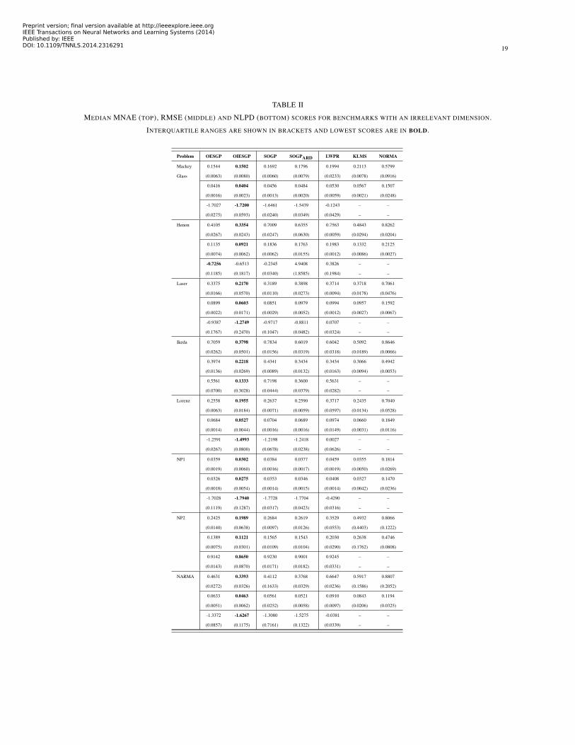
TABLE II
MEDIAN MNAE (TOP), RMSE (MIDDLE) AND NLPD (BOTTOM) SCORES FOR BENCHMARKS WITH AN IRRELEVANT DIMENSION.
INTERQUARTILE RANGES ARE SHOWN IN BRACKETS AND LOWEST SCORES ARE IN BOLD.
Problem OESGP OIESGP SOGP SOGPARD LWPR KLMS NORMA
Mackey 0.1544 0.1502 0.1692 0.1796 0.1994 0.2113 0.5799
Glass (0.0063) (0.0080) (0.0060) (0.0079) (0.0233) (0.0078) (0.0916)
0.0416 0.0404 0.0456 0.0484 0.0530 0.0567 0.1507
(0.0016) (0.0023) (0.0013) (0.0020) (0.0059) (0.0021) (0.0248)
-1.7027 -1.7200 -1.6461 -1.5439 -0.1243 – –
(0.0275) (0.0593) (0.0240) (0.0349) (0.0429) – –
Henon 0.4105 0.3354 0.7009 0.6355 0.7563 0.4843 0.8262
(0.0267) (0.0243) (0.0247) (0.0630) (0.0059) (0.0294) (0.0204)
0.1135 0.0921 0.1836 0.1763 0.1983 0.1332 0.2125
(0.0074) (0.0062) (0.0062) (0.0155) (0.0012) (0.0086) (0.0027)
-0.7256 -0.6513 -0.2345 4.9408 0.3826 – –
(0.1185) (0.1817) (0.0340) (1.8585) (0.1984) – –
Laser 0.3375 0.2170 0.3189 0.3898 0.3714 0.3718 0.7061
(0.0166) (0.0570) (0.0110) (0.0273) (0.0094) (0.0178) (0.0476)
0.0899 0.0603 0.0851 0.0979 0.0994 0.0957 0.1592
(0.0022) (0.0171) (0.0029) (0.0052) (0.0012) (0.0027) (0.0067)
-0.9387 -1.2749 -0.9717 -0.8811 0.0707 – –
(0.1767) (0.2470) (0.1047) (0.0482) (0.0324) – –
Ikeda 0.7059 0.3798 0.7834 0.6019 0.6042 0.5092 0.8646
(0.0262) (0.0501) (0.0156) (0.0319) (0.0318) (0.0189) (0.0066)
0.3974 0.2218 0.4341 0.3434 0.3434 0.3066 0.4942
(0.0136) (0.0269) (0.0089) (0.0132) (0.0163) (0.0094) (0.0053)
0.5561 0.1333 0.7198 0.3600 0.5631 – –
(0.0700) (0.3028) (0.0444) (0.0379) (0.0282) – –
Lorenz 0.2558 0.1955 0.2637 0.2590 0.3717 0.2435 0.7040
(0.0063) (0.0184) (0.0071) (0.0059) (0.0597) (0.0134) (0.0528)
0.0684 0.0527 0.0704 0.0689 0.0974 0.0660 0.1849
(0.0014) (0.0044) (0.0016) (0.0016) (0.0149) (0.0031) (0.0116)
-1.2591 -1.4993 -1.2198 -1.2418 0.0027 – –
(0.0267) (0.0800) (0.0678) (0.0238) (0.0626) – –
NP1 0.0359 0.0302 0.0384 0.0377 0.0459 0.0355 0.1814
(0.0019) (0.0060) (0.0016) (0.0017) (0.0019) (0.0050) (0.0269)
0.0326 0.0275 0.0353 0.0346 0.0408 0.0327 0.1470
(0.0018) (0.0054) (0.0014) (0.0015) (0.0014) (0.0042) (0.0236)
-1.7028 -1.7940 -1.7728 -1.7704 -0.4290 – –
(0.1119) (0.1287) (0.0317) (0.0423) (0.0316) – –
NP2 0.2425 0.1989 0.2684 0.2619 0.3529 0.4932 0.8066
(0.0140) (0.0638) (0.0097) (0.0126) (0.0553) (0.4403) (0.1222)
0.1389 0.1121 0.1565 0.1543 0.2030 0.2638 0.4746
(0.0075) (0.0301) (0.0109) (0.0104) (0.0290) (0.1762) (0.0808)
0.9142 0.8650 0.9230 0.9001 0.9245 – –
(0.0143) (0.0870) (0.0171) (0.0182) (0.0331) – –
NARMA 0.4631 0.3393 0.4112 0.3768 0.6647 0.5917 0.8807
(0.0272) (0.0326) (0.1633) (0.0329) (0.0236) (0.1586) (0.2052)
0.0633 0.0463 0.0561 0.0521 0.0910 0.0843 0.1194
(0.0051) (0.0062) (0.0252) (0.0058) (0.0097) (0.0206) (0.0325)
-1.3372 -1.6267 -1.3080 -1.5275 -0.0381 – –
(0.0857) (0.1175) (0.7161) (0.1322) (0.0339) – –
Preprint version; final version available at http://ieeexplore.ieee.orgIEEE Transactions on Neural Networks and Learning Systems (2014)Published by: IEEEDOI: 10.1109/TNNLS.2014.2316291

20
OESGP
OIESGP
SOGP
SOGPARD
LWPR
KLMS
NORMA
OESGP
OIESGP
SOGP
SOGPARD
LWPR
KLMS
NORMA
10−4
10−3
10−4
10−2
10−4
10−2
0.001
0.01
Mackey-Glass Henon Laser Ikeda Lorenz NP1 NP2 NARMA-10
Tra
inin
gTe
stin
g
Benchmark
Irre
lev
an
t D
ime
ns
ion
CP
U T
ime
Pe
r It
era
tio
n (
s)
Computational Time (in seconds) for Testing and Training
Tra
inin
gTe
stin
gT
rain
ing
Te
stin
g
Fig. 7. CPU time per iteration for testing and training. Overall, LWPR was the fastest algorithm for a majority of the problems considered.
Among the online GPs, the full ARD kernel was the most expensive to train and the isotropic kernel was the cheapest. The OIESGP was on
average cheaper than the OESGP for predictions, but required longer optimisation periods and hence, higher average training time.
−1
0
1 −1
0
1
−1
0
1
y t
s1,t s2,t
State Aliasing Due to Projected Noisy Observations
A
B
(a)
yt
Kernel Density Plot of Data Generated
by the Rotating Dynamical System
y t+1
Bi-modality of the Empirical
Conditional Distribution
yt+1
p(y
t+1|y
t)
0
0.5
1.0
−2 −1 0 1
(b)
p(y
t+1|y
t,y
t−1)
Kernel Density Plot with 1-step
Coordinate Delay Embedding
yt
y t+1
yt+1yt−1
0
1
2
3
4
5
0.6 0.8 1.0 1.2
Uni-modality of the Empirical
Conditional Distribution
(c)
Fig. 8. (a) True states of the rotating dynamical system live on a unit circle but give rise to noisy observations. Two distinct sets of points,
A and B, give rise to the same observation (the plane yt = 0) (b) The probability of the next observation conditioned upon the current one
is bi-modal, violating assumptions made by typical regression methods. This bi-modality occurs because of state aliasing caused by partial
observations. (c) A coordinate delay embedding reconstructs the state space sufficiently well that uni-modality is recovered and predictions can
be performed accurately.
log p(yt|yt, σ2t ) =
12 log σ
2t +
(yt−yt)2
2σ2
t
+ 12 log 2π. Unlike the two aforementioned error scores, the NLPD penalises
methods which are overconfident.
B. Accuracy Results
Let us first consider the noisy prediction problems without any irrelevant inputs. Table I summarises the three
error scores obtained by each of the algorithms. Overall, the GP methods outperformed the other algorithms on all
of the benchmarks except for the NP1 problem, where LWPR obtains the lowest MNAE and RMSE error scores.
Among the online GPs, the OESGP and OIESGP obtained the best scores on a majority of the benchmarks.
Preprint version; final version available at http://ieeexplore.ieee.orgIEEE Transactions on Neural Networks and Learning Systems (2014)Published by: IEEEDOI: 10.1109/TNNLS.2014.2316291

21
Interestingly, the simple SOGP with the isotropic Gaussian kernel also performed comparably well on the Mackey-
Glass, Ikeda, NP2 and NARMA-10 benchmarks, echoing recent results [23], [41] that complex reservoirs are not
necessary for certain prediction tasks. We had expected the SOGP with the full ARD kernel to realise lower errors
than the isotropic kernel because the additional lengthscale parameters would allow a better fit to the given problems.
However, this only occurred for the Henon, Laser and Ikeda benchmarks. This discrepancy may be explained by
the fact that the full ARD kernel required an optimisation over a larger hyperparameter space and would settle into
local minima (or not converge within the maximum number of iterations set).
The full benefit of the OIESGP with the recursive ARD kernel is evidenced by its performance on the problems
with irrelevant inputs (Table II); the OIESGP outperforms all the other methods, including the OESGP, in terms of
the error scores on all the problems; results are statistically significant at α = 0.05 level (Bonferroni corrected).
C. Computational Costs
Comparing computational costs, LWPR remains the overall fastest algorithm in terms of CPU time; average
training and testing times are shown in Fig. 7. That said, during our tests, we had to fine-tune LWPR parameters
when the grid-search took days of computation time under certain parameterisations. Among the online GP methods,
the isotropic Gaussian was the most rapid kernel, as expected. Contrasting OIESGP with OESGP, although training
was more expensive on the benchmarks with irrelevant dimensions (due to the longer optimisation periods), the
OIESGP produced predictions 20% faster on all the benchmarks except NP1 and NARMA-10 with irrelevant
dimensions.
VII. DISCUSSION: A DYNAMICAL SYSTEMS PERSPECTIVE
There are two notable findings obtained from our experiments. First, the isotropic Gaussian produces results
comparable to more complex methods on the one-step prediction task with dynamical systems. Second, the OIESGP
was decidedly more accurate than the other methods on the problems with irrelevant dimensions. In this section,
we try to understand the reasons for these observations from the perspective of dynamical systems theory.
An important result in the field of non-linear dynamical systems is Taken’s Embedding Theorem [12], which
states that the sliding-window (delay vector) constructed from single observations is an embedding — a one-
to-one mapping between manifolds — whenever the length of the delay vector is larger than twice the instrinsic
dimensionality of original space. Informally, a sufficiently long sliding window reconstructs the state-space such that
topological properties are preserved. Although Taken’s original statement assumed infinite precision observations
with no noise, this result has been extended to systems with observation and dynamical noise [42], [43].
As a concrete example, consider a simple linear dynamical system consisting of a rotating two-dimensional state
st by a fixed angle θ via iterative application of T to an initial state vector s0.
st+1 = Tst (54)
yt = Ost + ǫy (55)
Preprint version; final version available at http://ieeexplore.ieee.orgIEEE Transactions on Neural Networks and Learning Systems (2014)Published by: IEEEDOI: 10.1109/TNNLS.2014.2316291

22
State Delay Vector
Observation Delay Vector
Reservoir
I(y
t+1 | f
R (
ht )
)
0.5
1.0
1.5
Delay Length / Reservoir Size
0 2 4 6 8 10
Mutual Information between Varying History
Representation Lengths and Next Observation
I(y
t+1,φ
(ht))
Fig. 9. The mutual information between the next observation (to be predicted) and the delay vector (sliding-window) grows with with the delay
length approaching that of the underlying state. As we would expect, a delay vector constructed using the underlying state does not increase
the mutual information. The reservoir shows a different initial profile; a increase from 3 to 4 neurons results a sudden jump in informativeness.
where
T =
cos θ − sin θ
sin θ cos θ
O =
1 0
0 0
and θ = 0.1, s0 = [0, 1]⊤, ǫy ∼ N (0, 0.1). In Figure 8b, we see that standard regression on the observations will fail
to produce accurate predictions since the distribution is generally bi-modal; as a partial observation, yt only contains
limited information about the underlying state. As Fig. 8a shows, contaminated states lead to state aliasing; two
distinct state sets A and B can generate observations yt ≈ 0 (illustrated by the plane). This phenomena undermines
predictability of the system.
However, a sufficiently long history of the observed time-series — the embedding — preserves important
properties. In this example, a simple one-step delay vector reconstructs the state space sufficiently well such that
uni-modality of conditional probability is recovered (Fig. 8c).
Taken’s Theorem gives a reason why, for the basic prediction problems, the isotropic Gaussian with a sliding-
window performed well: using a window permits the GP to operate in a space topologically similar to the original
state space. Indeed, the reservoirs used in echo-state networks and the OESGP can be viewed as reconstructions.
Computing the mutual information (MI) between the next observation and the delay vector and reservoir recon-
structions (Fig. 9) allows us to quantitatively compare the informativeness of the different representations. For our
sample problem, the sliding-window and reservoirs have different MI profiles as the size of the representation is
increased. While the increase is more gradual for the delay vector, the reservoir requires a minimum size — a
“tipping point” — before sufficient information was available.
A. The Problem of False Neighbours
As to the second question of why the introduction of an irrelevant dimension hampered the algorithms except
the OIESGP, we consider the issue of false neighbours [13], used in state-space reconstruction to find the optimal
Preprint version; final version available at http://ieeexplore.ieee.orgIEEE Transactions on Neural Networks and Learning Systems (2014)Published by: IEEEDOI: 10.1109/TNNLS.2014.2316291

23
−0.3
−0.2
−0.1
0
0.1
0.2
0.3
0.4
−0.2−0.100.10.20.3
X
Y
Fig. 10. The Lazy-8 Learning-by-Demonstration experimental setup with the Nao humanoid robot with the collected trajectories [45]. Our goal
is to learn the (shoulder pitch/roll, elbow yaw/roll) joint velocities needed to produce the figure-8’s demonstrated.
sliding-window dimension.
The idea itself is straightforward: as our simple rotating system demonstrates, partial observations with noise
project states from their true high-dimensional spaces into neighbourhoods that they do not truly belong; as such,
these projected points have neighbours that may be from other regions of the space.
This has consequences for GPs (and other non-parametric methods) that rely on the notion of similarity between
the inputs as represented by the kernel function. Irrelevant dimensions exacerbate the problem of false neighbours
because the “extra” dimensions factor into the kernel, distorting distances and thus, decreasing prediction accuracy.
As such, we can interpret SNGD using the recursive ARD kernel as a “moulding” of the similarities (via the
hyperparameters) using the predictability of the system to approximate the topological properties of the original
space. Although the full ARD kernel with sufficiently long window offers this feature, the parameter space employed
is far larger. In a practical sense, the OIESGP strikes a balance between having too many parameters (the full ARD
and reservoir) and having too few (the isotropic Gaussian).
VIII. CASE STUDIES IN ONLINE ROBOT LEARNING BY DEMONSTRATION
In this section, we describe two case studies applying our methods to robot Learning-by-Demonstration (LbD),
which addresses the challenging task of developing robot control policies — mappings from states to actions. As
compared to developing policies by-hand, LbD methods derive policies from teacher demonstrations, which is often
more intuitive than hand-coding specific behaviours. This has inherent benefits: it enables rapid prototyping and
allows non-roboticists to participate in policy development [44].
A. Lazy-8 with the Nao Humanoid Robot
Our first case study is an online robot learning by demonstration scenario involving the Nao humanoid robot
(with 27 degrees of freedom) learning to draw the figure 8 (Fig. 10). This deceptively-simple Lazy-8 problem is a
classic benchmark problem because learning the joint velocity control to reproduce the demonstrated figures on a
real-world robot is non-trivial. As shown in Fig. 11, not only is the observed data noisy, the demonstrations have
different origin points and are limited in length.
Preprint version; final version available at http://ieeexplore.ieee.orgIEEE Transactions on Neural Networks and Learning Systems (2014)Published by: IEEEDOI: 10.1109/TNNLS.2014.2316291

24
0 2 4 6 8 10−2
−1.5
−1
−0.5
0
0.5
1
1.5
0 2 4 6 8 10−0.03
−0.02
−0.01
0
0.01
0.02
0.03
Time (s)
Velo
cit
y (
rad
/s)
Jo
int
An
gle
(ra
d)
Time (s)
Joint Angles and Velocities for the Lazy-8 Experiment
Fig. 11. Joint angles and velocities for the four left arm joints; shoulder-pitch (blue), shoulder-roll (red), elbow-yaw (green), elbow-roll (black).
For our experiments, the raw angles (left) were inputs and velocities (right) were outputs. Best viewed in colour.
TABLE III
PREDICTION AND TRAJECTORY RECONSTRUCTION MSE FOR THE LAZY-8 EXPERIMENT. STANDARD DEVIATIONS ARE SHOWN IN
BRACKETS AND LOWEST SCORES ARE IN BOLD.
OESGP OIESGP LWPR OGMM OSMM
Trajectory 1.373 0.260 4.032 2.479 2.214
×10−3 (0.723) (0.151) (0.982) (1.389) (0.684)
Joint Velocity 1.172 0.279 1.750 1.808 1.411
×10−5 (0.512) (0.104) (0.376) (0.349) (0.188)
In our setup, we employed twelve kinesthetic demonstrations, whereby the goal is to predict the velocity controls
given the current joint angles. Here, we compare the performance of OESGP, OIESGP and LWPR. In addition, we
include recent results obtained using incremental versions of the Gaussian mixture model (OGMM) and Student t’s
mixture model (OSMM) [45]. To compare methods, we computed the mean-squared error in both the (reconstructed)
trajectory and joint spaces.
For each of the algorithms, we performed a grid-search over relevant parameters and report the best results
obtained. In summary, the OESGP used a reservoir with 50 neurons (0.1 connectivity with the hyperbolic transform
activation function), a spectral radius of 0.9 and leak rate of 0.95. The capacity, lengthscale and noise hyperparam-
eters were set at 100, 1.0 and 0.01 respectively. The OIESGP was initialised with capacity 100, τ = 20, spatial
lengthscales of 2.0, a temporal lengthscale of 1.2 and a noise value of 0.01. The best LWPR model used a initial
diagonal distance matrix of 1.0 with meta learning enabled (rate of 50), penalty 10−4 and a sliding window of 20
time-steps.
Table III summarises the MSE scores obtained by each of the algorithms. Both our reservoir-inspired methods
perform better than the competing methods with the OIESGP achieving the best scores. Indeed, OIESGP’s error
scores are an order of magnitude lower than the compared algorithms for both the trajectory (0.260×10⁻³) and joint
(0.279× 10⁻⁵) measures. Comparing computational costs, OESGP and OIESGP took 5.3× 10⁻⁴ and 6.1× 10⁻⁴
seconds per iteration respectively, both faster than LWPR (4.1 × 10⁻³ s) and most importantly, fast enough for
Preprint version; final version available at http://ieeexplore.ieee.orgIEEE Transactions on Neural Networks and Learning Systems (2014)Published by: IEEEDOI: 10.1109/TNNLS.2014.2316291

25
x
yz
++
+
Fig. 12. Falcon placement on the ARTY smart wheelchair with a sample demonstration using the 3-DoF Falcon Haptic Controller; the x-axis
controlled the forward and backward speeds where else the y-axis controlled the turning velocities. The z-axis was not used in this study.
6.2 m
S
F
−3−2−10123
−3
−2.5
−2
−1.5
−1
−0.5
0
0.5
1
1.5
SF
Recorded TrajectoriesExperimental Area
Fig. 13. Experimental area for wheelchair driving case-study with recorded trajectories. Demonstrators were told to drive from S to F, passing
through the waypoints (blue dots).
real-time performance.
B. Haptic Control and the ARTY Smart Wheelchair
For our second case study, we focus on the problem of assisted mobility for young children. Our overarching
goal is to provide a smart wheelchair for young children that not only provides assisted mobility, but also functions
as a training tool. In this work, we experiment with a 3-DoF Falcon haptic controller (Fig. 12) on the ARTY smart
wheelchair with the aim of providing haptic guidance. Instead of hard-coding a track (e.g., in [46]), we teach the
smart wheelchair to drive a lap and provide the corresponding haptic feedback.
The objective was to model the 3-dimensional position of the Falcon “ball” controller (bx, by, bz), given the
pose and velocity of the wheelchair — 2-D map coordinates (mx, my), direction angle mα, translational velocity
vs and turning velocity vα. The pose and velocities obtained using adaptive Monte-carlo localisation (AMCL) and
gyroscope readings respectively. Only the X and Y Falcon-axes were used for controlling the wheelchair; the X-axis
controlled the speed and the Y-axis affected the turning rate. Our test environment was an office-space and five
demonstrator laps were collected with the sampled trajectories shown in Fig. 13.
For this experiment, we compared the OESGP, OIESGP and LPWR algorithms. As before, we performed a
Preprint version; final version available at http://ieeexplore.ieee.orgIEEE Transactions on Neural Networks and Learning Systems (2014)Published by: IEEEDOI: 10.1109/TNNLS.2014.2316291

26
TABLE IV
PREDICTION RMSE FOR THE WHEELCHAIR DRIVING TASK. STANDARD DEVIATIONS ARE SHOWN IN BRACKETS AND LOWEST SCORES
ARE IN BOLD.
OESGP OIESGP LWPR
X-axis 1.742 1.669 1.956
RMSE ×10−1 (0.285) (0.356) (0.370)
Y-axis 2.815 2.570 3.349
RMSE ×10−1 (0.717) (0.613) (0.840)
Z-axis 1.729 1.715 1.487
RMSE ×10−1 (0.723) (0.716) (0.809)
simple grid-search to find the best model for each algorithm. The best OESGP model used a 50-neuron reservoir
with 0.1 connectivity, input scaling of 0.5 and spectral radius of 0.9. The characteristic and temporal lengthscales
were set at 1.0 and 1.2 respectively. For OIESGP, the characteristic and temporal lengthscales were 5 and 1.2 with
τ = 5. The prior noise for both OESGP and OIESGP was 0.05. LWPR used a sliding window of 5 time-steps and
an initial distance metric of 0.5, a learning rate of 1 and meta-learning enabled. The methods were compared using
the five-fold cross-validation RMSE.
Table IV summarises our results; the lowest average RMSE scores for the X and Y axes were obtained by
OIESGP, while the best score for the Z-axis was obtained by LWPR. However, given the error standard deviations,
both the OIESGP and OESGP performed similarly well; 15 − 20% lower errors compared to LWPR for the two
controlling axes. Fig. 14 illustrates a representative prediction profile for the OIESGP algorithm, showing the method
is able to learn from teaching samples to provide control signals very similar to the human demonstrator. Regarding
computational times, OIESGP operated at 7.421 × 10⁻⁴ seconds per iteration, slightly slower than LWPR which
required 6.0390 × 10⁻⁴ s per iteration. OESGP was the slowest method at 1.034 × 10⁻³ seconds. That said, all
three methods were faster than the 10Hz requirement.
In summary, the OESGP and OIESGP performed well relative to LWPR for the task of learning to control the
Falcon haptic controller, and hence, the smart wheelchair to drive around a track. Either of the methods can be
used in a LbD system whereby an occupational therapist can easily change training tracks via demonstration to
better suit different users (or the same user at different stages of his/her development).
IX. CONCLUSIONS AND FUTURE WORK
In this paper, we presented finite and infinite variants of the online Echo-state Gaussian process, which are iterative
temporal learners with fixed maximum computational and storage budget. The OESGP uses a fixed reservoir, while
the OIESGP uses recursive kernels inspired by reservoirs with an infinite number of neurons. We introduced a new
recursive kernel with varying spatial lengthscales, which can be optimised iteratively using SNGD.
As demonstrated in tests, this yields an adaptive method better capable of processing irrelevant dimensions.
Preprint version; final version available at http://ieeexplore.ieee.orgIEEE Transactions on Neural Networks and Learning Systems (2014)Published by: IEEEDOI: 10.1109/TNNLS.2014.2316291

27
Time (s)
x
y
z
Sample OIESGP Prediction with Demonstration #2
Fig. 14. Sample predictions for each of the Falcon axes with the demonstration values shown as black dashed lines.
Experiments on benchmark problems demonstrated the efficacy of the reservoir-based GPs, particularly the OIESGP
over using the isotropic and full ARD kernels, as well as state-of-the-art methods including LWPR, NORMA and
KLMS. Taking a larger perspective, we believe both the OESGP and OIESGP will be effective “building blocks”
in learning systems that are expected to work in real-world scenarios.
In this work, we presented two case studies in LbD; learning Lazy-8s with the Nao humanoid robot and haptic
control with the ARTY smart wheelchair. We observed that the OESGP and OIESGP surpassed other leading
methods, achieving higher accuracies while being fast enough for real-time use.
We envision that this work can be extended in several ways; for example, the algorithms can be used in a mixture
of experts model, which may increase modelling power, while reducing the computational costs associated with the
optimisation process. Also, for non-stationary time-series, a forgetting factor [8] can be easily assimilated into our
methods. Moreover, to improve accuracy with very small basis vector sets, we may consider “freely-moving” basis
vectors [47]. Although our experiments show that our methods can perform well even when inputs are noisy, GPs
in their theoretical formulation assume noiseless inputs. Learning with inputs contaminated with Gaussian noise
and a squared exponential kernel leads to a “corrected” kernel with increased lengthscales [48]. Intuitively, the
same outcome should hold for our recursive ARD kernel but this has yet to be rigorously proven. It would also be
interesting to apply our methods in more complex architectures such as HAMMER [49], which would allow for
Preprint version; final version available at http://ieeexplore.ieee.orgIEEE Transactions on Neural Networks and Learning Systems (2014)Published by: IEEEDOI: 10.1109/TNNLS.2014.2316291

28
attention driven learning, and deep models [50] for modelling long-term spatio-temporal correlations.
ACKNOWLEDGMENT
The authors thank members of the Personal Robotics Lab at Imperial College London for their help, particularly
Dimitrios Korkinof for his valuable feedback and assistance with the Nao. This work was supported in part by the
EU FP7 project ALIZ-E under Grant 248116.
REFERENCES
[1] H. Soh and Y. Demiris, “Iterative Temporal Learning and Prediction with the Sparse Online Echo State Gaussian Process,” in IEEE
International Joint Conference on Neural Networks, 2012, pp. 1–8.
[2] H. Soh, Y. Su, and Y. Demiris, “Online spatio-temporal Gaussian process experts with application to tactile classification,” in IEEE/RSJ
International Conference on Intelligent Robots and Systems, 2012, pp. 4489–4496.
[3] H. Jaeger, “The ”echo state” approach to analysing and training recurrent neural networks,” German National Research Center for
Information Technology, Bremen, Tech. Rep. 148, 2001.
[4] L. Csato and M. Opper, “Sparse On-Line Gaussian Processes,” Neural Computation, vol. 14, no. 3, pp. 641–668, March 2002.
[5] M. Hermans and B. Schrauwen, “Recurrent Kernel Machines: Computing with Infinite Echo State Networks,” Neural Computation, vol. 24,
no. 1, pp. 104–133, 2011.
[6] R. Neal, Bayesian learning for neural networks, ser. Lecture Notes in Statistics. Springer Verlag, 1996, no. 118.
[7] S. I. Amari, “Natural gradient works efficiently in learning,” Neural computation, vol. 10, no. 2, pp. 251–276, 1998.
[8] S. Van Vaerenbergh, M. Lazaro-Gredilla, and I. Santamarıa, “Kernel Recursive Least-Squares Tracker for Time-Varying Regression,” IEEE
Transactions on Neural Networks and Learning Systems, vol. 23, no. 8, pp. 1313–1326, 2012.
[9] Y. Engel, S. Mannor, and R. Meir, “The Kernel Recursive Least-Squares Algorithm,” IEEE Transactions on Signal Processing, vol. 52,
no. 8, pp. 2275–2285, Aug. 2004.
[10] S. Vijayakumar, A. D’souza, and S. Schaal, “Incremental online learning in high dimensions,” Neural Computation, vol. 17, no. 12, pp.
2602–2634, 2005.
[11] W. Liu, P. Pokharel, and J. Principe, “The Kernel Least-Mean-Square Algorithm,” IEEE Transactions on Signal Processing, vol. 56, no. 2,
pp. 543–554, 2008.
[12] F. Takens, “Detecting strange attractors in turbulence,” in Dynamical systems and turbulence. Springer, 1981, pp. 366–381.
[13] H. Kantz and T. Schreiber, Nonlinear Time Series Analysis. Cambridge University Press, 2003, vol. 7.
[14] H. Soh and Y. Demiris, “Towards early mobility independence: An intelligent paediatric wheelchair with case studies,” in IROS 2012
Workshop on Progress, Challenges and Future Perspectives in Navigation and Manipulation Assistance for Robotic Wheelchairs, 2012.
[15] A. M. Schafer and H. G. Zimmermann, “Recurrent neural networks are universal approximators,” in Artificial Neural Networks–ICANN
2006. Springer, 2006, pp. 632–640.
[16] D. Rumelhart, G. Hinton, and R. Williams, “Learning representations by back-propagating errors,” Nature, vol. 323, no. 6088, pp. 533–536,
1986.
[17] P. J. Werbos, “Generalization of backpropagation with application to a recurrent gas market model,” Neural Networks, vol. 1, no. 4, pp.
339 – 356, 1988.
[18] R. J. Williams and D. Zipser, “A learning algorithm for continually running fully recurrent neural networks,” Neural Computation, vol. 1,
no. 2, pp. 270–280, June 1989.
[19] W. Maass, T. Natschlager, and H. Markram, “Real-time computing without stable states: A new framework for neural computation based
on perturbations,” Neural computation, vol. 14, no. 11, pp. 2531–2560, 2002.
[20] M. Lukosevicius and H. Jaeger, “Reservoir computing approaches to recurrent neural network training,” Computer Science Review, vol. 3,
no. 3, pp. 127–149, 2009.
[21] H. Jaeger, “Adaptive nonlinear system identification with echo state networks,” in Advances in Neural Information Processing Systems,
2003, pp. 593–600.
Preprint version; final version available at http://ieeexplore.ieee.orgIEEE Transactions on Neural Networks and Learning Systems (2014)Published by: IEEEDOI: 10.1109/TNNLS.2014.2316291

29
[22] Z. Deng and Y. Zhang, “Collective behavior of a small-world recurrent neural system with scale-free distribution,” IEEE Transactions on
Neural Networks, vol. 18, no. 5, pp. 1364 –1375, Sept. 2007.
[23] A. Rodan and P. Tino, “Minimum complexity echo state network,” IEEE Transactions on Neural Networks, vol. 22, no. 1, pp. 131 –144,
jan. 2011.
[24] P. Kountouriotis, D. Obradovic, S. Goh, and D. Mandic, “Multi-step forecasting using echo state networks,” in The International Conference
on Computer as a Tool (EUROCON 2005), vol. 2. IEEE, 2005, pp. 1574–1577.
[25] R. E. Kalman et al., “A new approach to linear filtering and prediction problems,” Journal of Basic Engineering, vol. 82, no. 1, pp. 35–45,
1960.
[26] C. E. Rasmussen and C. K. I. Williams, Gaussian Processes for Machine Learning. The MIT Press, 2006.
[27] S. Chatzis and Y. Demiris, “Echo State Gaussian Process,” IEEE Transactions on Neural Networks, vol. 22, no. 9, pp. 1435 –1445, Sept.
2011.
[28] J. Quinonero Candela and C. E. Rasmussen, “A unifying view of sparse approximate gaussian process regression,” Journal of Machine
Learning Research, vol. 6, pp. 1939–1959, December 2005.
[29] M. Opper, “A Bayesian approach to on-line learning,” Online Learning in Neural Networks, pp. 363–378, 1998.
[30] L. Csato, “Gaussian processes: iterative sparse approximations,” Ph.D. dissertation, Aston University, 2002.
[31] F. Vivarelli and C. Williams, “Discovering hidden features with gaussian processes regression,” Advances in Neural Information Processing
Systems, pp. 613–619, 1999.
[32] S. Geisser and W. F. Eddy, “A predictive approach to model selection,” Journal of the American Statistical Association, vol. 74, no. 365,
pp. 153–160, 1979.
[33] N. Le Roux, P. A. Manzagol, and Y. Bengio, “Topmoumoute online natural gradient algorithm,” in Advances in Neural Information
Processing Systems, vol. 20, 2007, pp. 849–856.
[34] S. I. Amari, H. Park, and K. Fukumizu, “Adaptive method of realizing natural gradient learning for multilayer perceptrons,” Neural
Computation, vol. 12, no. 6, pp. 1399–1409, 2000.
[35] M. Seeger, C. Williams, and N. Lawrence, “Fast forward selection to speed up sparse gaussian process regression,” in Ninth Intl. Workshop
on Artificial Intelligence and Statistics, vol. 9, 2003.
[36] L. Bottou, “Stochastic gradient descent tricks,” in Neural Networks: Tricks of the Trade. Springer, 2012, pp. 421–436.
[37] A. F. Atiya and A. G. Parlos, “New results on recurrent network training: Unifying the algorithms and accelerating convergence,” IEEE
Transactions on Neural Networks, vol. 11, no. 3, pp. 697–709, 2000.
[38] J. Kivinen, A. Smola, and R. Williamson, “Online learning with kernels,” IEEE Transactions on Signal Processing, vol. 52, no. 8, pp.
2165 – 2176, Aug. 2004.
[39] E. Wen, “Time series data,” 2011. [Online]. Available: http://web.cecs.pdx.edu/%7Eericwan/time-series-data.html
[40] D. Verstraeten and M. Wardermann, “Reservoir computing toolbox.” [Online]. Available: http://reslab.elis.ugent.be/rctoolbox
[41] T. Strauss, W. Wustlich, and R. Labahn, “Design strategies for weight matrices of echo state networks,” Neural Computation, vol. 24,
no. 12, pp. 3246–3276, Dec. 2012.
[42] M. Casdagli, S. Eubank, J. D. Farmer, and J. Gibson, “State space reconstruction in the presence of noise,” Physica D: Nonlinear
Phenomena, vol. 51, no. 1, pp. 52–98, 1991.
[43] J. Stark, D. Broomhead, M. Davies, and J. Huke, “Delay embeddings for forced systems. ii. stochastic forcing,” Journal of Nonlinear
Science, vol. 13, no. 6, pp. 519–577, 2003.
[44] B. D. Argall, S. Chernova, M. Veloso, and B. Browning, “A survey of robot learning from demonstration,” Robotics and Autonomous
Systems, vol. 57, no. 5, pp. 469–483, May 2009.
[45] D. Korkinof and Y. Demiris, “Online Quantum Mixture Regression for Trajectory Learning by Demonstration,” in IEEE/RSJ International
Conference on Intelligent Robots and Systems (Accepted), 2013.
[46] L. Marchal-Crespo, J. Furumasu, and D. J. Reinkensmeyer, “A robotic wheelchair trainer: design overview and a feasibility study,” Journal
of NeuroEngineering and Rehabilitation, vol. 7, p. 40, 2010.
[47] E. Snelson and Z. Ghahramani, “Sparse gaussian processes using pseudo-inputs,” in Advances in Neural Information Processing Systems
18, 2006, pp. 1257–1264.
Preprint version; final version available at http://ieeexplore.ieee.orgIEEE Transactions on Neural Networks and Learning Systems (2014)Published by: IEEEDOI: 10.1109/TNNLS.2014.2316291

30
[48] A. Girard, “Approximate methods for propagation of uncertainty with gaussian process model,” Ph.D. dissertation, University of Glasgow,
Glasgow, UK, 2004.
[49] Y. Demiris and B. Khadhouri, “Hierarchical attentive multiple models for execution and recognition of actions,” Robotics and Autonomous
Systems, vol. 54, no. 5, pp. 361–369, 2006.
[50] Y. Bengio, “Learning deep architectures for AI,” Foundations and trends R© in Machine Learning, vol. 2, no. 1, pp. 1–127, 2009.
Preprint version; final version available at http://ieeexplore.ieee.orgIEEE Transactions on Neural Networks and Learning Systems (2014)Published by: IEEEDOI: 10.1109/TNNLS.2014.2316291