Seediscussions,stats,andauthorprofilesforthispublicationat:https://www.researchgate.net/publication/290036927

Spatiallyvaryingcoefficientmodelsinrealestate:Eigenvectorspatialfilteringandalternativeapproaches

ARTICLEinCOMPUTERSENVIRONMENTANDURBANSYSTEMS·MAY2016

ImpactFactor:1.79·DOI:10.1016/j.compenvurbsys.2015.12.002

READS

4

2AUTHORS,INCLUDING:

MarcoHelbich

UtrechtUniversity

62PUBLICATIONS411CITATIONS

SEEPROFILE

Allin-textreferencesunderlinedinbluearelinkedtopublicationsonResearchGate,

lettingyouaccessandreadthemimmediately.

Availablefrom:MarcoHelbich

Retrievedon:14January2016

Computers, Environment and Urban Systems 57 (2016) 1–11

Contents lists available at ScienceDirect

Computers, Environment and Urban Systems

j ourna l homepage: www.e lsev ie r .com/ locate /ceus

Spatially varying coefficient models in real estate: Eigenvector spatialfiltering and alternative approaches

Marco Helbich a,⁎, Daniel A. Griffith b

a Department of Human Geography and Spatial Planning, Utrecht University, Heidelberglaan 2, 3584 CS, Utrecht, The Netherlandsb School of Economic, Political and Policy Sciences, University of Texas at Dallas, 800 W. Campbell Rd, Richardson, TX 75080-3021, USA

⁎ Corresponding author.E-mail address: m.helbich@uu.nl (M. Helbich).

http://dx.doi.org/10.1016/j.compenvurbsys.2015.12.0020198-9715/© 2015 Elsevier Ltd. All rights reserved.

a b s t r a c t

a r t i c l e i n f o

Article history:Received 4 March 2015Received in revised form 23 October 2015Accepted 8 December 2015Available online xxxx

Real estate policies in urban areas require the recognition of spatial heterogeneity in housing prices to account forlocal settings. In response to the growing number of spatially varying coefficient models in housing applications,this study evaluated four models in terms of their spatial patterns of local parameter estimates, multicollinearitybetween local coefficients, and their predictive accuracy, utilizing housing data for the metropolitan area of Vienna(Austria). The comparison covered the spatial expansion method (SEM), moving window regression (MWR),geographically weighted regression (GWR), and genetic algorithm-based eigenvector spatial filtering (ESF), anapproach that had not previously been employed in real estate research. The results highlight the followingstrengths and limitations of each method: 1) In contrast to SEM, MWR, and GWR, ESF depicts more localizedpatterns of the parameter estimates and does not smooth local particularities. 2) ESF is less affected bymulticollinearity between the local parameter estimates than MWR, GWR, and SEM. 3) Even though thein-sample explanatory power and prediction accuracy of ESF is superior compared to the competitors, repeatedsampling indicates a limited out-of-sample fit and prediction accuracy, suggesting over-fitting tendencies. 4) Theapplication of ESF is less intuitive than MWR and GWR, which are available off-the-shelf.

© 2015 Elsevier Ltd. All rights reserved.

Keywords:Hedonic modelsHousingEigenvector spatial filteringSpatial expansion methodMoving window regressionGeographically weighted regressionPrediction accuracy

1. Introduction

Interest in hedonicmodels that consider the spatial heterogeneity ofpricing effects to explore real estate markets in urban areas has grownrapidly (Helbich, Brunauer, Hagenauer, & Leitner, 2013; Lu, Charlton,Harris, & Fotheringham, 2014). Conventional global hedonic modelsassume a unitary housing market across space that can be modeledthrough a single price function being representative throughout acity (Bitter, Mulligan, & Dall'erba, 2007). Suchmodels are increasing-ly questioned due to their unrealistic simplification of housingmarkets (McMillen & Redfearn, 2010). As a consequence, localhedonic models emerged as an alternative to explore spatiallyvarying housing prices. Even though spatially varying pricing effects arecongruent with urban economic theory (Redfearn, 2009) referring to“micro-market effects” (Sunding& Swoboda, 2010, p. 558), and emergingwhere local legislation and policy regulation are effective (Helbich,Brunauer, Vaz, & Nijkamp, 2014), their incorporation in hedonic modelsconstitutes a methodological challenge. However, neglecting spatialheterogeneity might have serious consequences for model estimation,such as biased regression coefficients, resulting in inappropriate conclu-sions (LeSage & Pace, 2009; Páez, Fei, & Farber, 2008). No less important,

since policy strategies rely on suchmodels, it is critical for decisionmakersto have models that have the highest fit (Ahn, Byun, Oh, & Kim, 2012;Bourassa, Cantoni, & Hoesli, 2010) and that inform them properly aboutlocal housing market conditions, for example through visualizations ofspatially varying marginal prices (Ali, Partridge, & Olfert, 2007). Suchmodels also reduce the risk for mortgage lenders and appraisal agenciesby obviating loan losses and erroneous real estate assessments.

Despite these appealing methodological and practical advantages oflocalized models (e.g. Fotheringham, Charlton, & Brunsdon, 2002;Griffith, 2008) in real estate applications, there is still disagreementover which local hedonic approach is superior (Ahn et al., 2012). Inthis regard, comparative studies are helpful to contrast the merits ofdifferent modeling techniques, particularly in light of the increase inthe number of applications and the proliferation of new approaches(Páez et al., 2008). Until now, simulation experiments based on artificiallygenerated data with known properties have dominated the comparativeanalysis literature (e.g., Páez, Farber, & Wheeler, 2011). Even thoughsuch investigations greatly improve our knowledge of the advantagesand limitations of specific hedonic models, without linking them tomore complex real-world case studies, simulation studies cannot entirelyuncover their practical relevance. Consequently, empirical model assess-ments complementing simulations are essential. As model competitionoutcomes are data-dependent and might cause contradictory results,Bourassa et al. (2010) recommend that empirical comparisons utilize asingle dataset.

2 M. Helbich, D.A. Griffith / Computers, Environment and Urban Systems 57 (2016) 1–11

Therefore, the principal objective of this study was to address themodel performance of four spatially varying coefficient models using ahousing dataset for themetropolitan area of Vienna, Austria. As opposedto Farber and Yeates (2006) and Bitter et al. (2007), this studycompared SEM, MWR, and GWR by applying a more rigorous out-of-sample accuracy assessment, resulting in less optimistic results thanwhen using the R2 as performance measure. There are three reasonsfor selecting these models: their performance is good, they haveremarkable recognition in urban housing studies, and they support anenhanced understanding of local market conditions (e.g. Helbich et al.,2014; Kestens, Theriault, & Des Rosiers, 2006; Osland, 2010; Sunding& Swoboda, 2010). The second innovation was the introduction of ESFto model geographically varying relationships and to test the predictiveperformance of this approach relative to SEM, MWR, and GWR. It is thismodel, which had not previously been utilized in the context of hedonicmodeling, that makes this study not only of interest for urban analysis,but also of practical relevance to urban policymaking. Finally, as ESFgrounds on stepwise variable selection procedures which only test alimited number of variable combinations (i.e., the interaction terms be-tween the eigenvectors and housing predictors), a genetic algorithm-based approach had been proposed as alternative.

2. Spatial hedonic price analyses

The theoretical foundation of hedonic modeling is motivated byLancaster's (1966) theory of consumer utility, which argues that it isnot the good itself that generates utility, but the good's specificcharacteristics. Grounded in this notion, Rosen (1974) developedhedonic pricing theory, which explains that a house price is thesum of its utility-bearing characteristics. Housing is thus considereda heterogeneous good consisting of non-separable structural andneighborhood features (Malpezzi, 2003). Each of these characteristicshas its individual implicit price. Because property is fixed in space, ahousehold implicitly chooses a bundle of different goods by selectinga specific house, seeking to maximize its utility. Hence, a household'spurchasing decision theoretically reflects an optimal configuration ofhousing attributes and their paid transaction price (Sheppard, 1997).

Hedonic analysis provides a well-established approach to decon-struct a total house price, and to determine corresponding marginalprices (Malpezzi, 2003). A hedonic equation and its associatedunknown parameters are estimated through non-spatial and spatialeconometric regression or geostatistical approaches (e.g., Anselin &Arribas-Bel, 2013; Kuntz & Helbich, 2014). Besides the specificationof the functional form (Helbich, Jochem, Mücke, & Höfle, 2013),spatial effects subsuming spatial autocorrelation (SAC) and spatial het-erogeneity, challenge model estimation (Dubin, 1998). Spatial effectsare deduced from the durability and spatial fixation of properties,questioning the validity of non-spatial regression (McMillen &Redfearn, 2010). Accordingly, by assuming spatial equilibrium betweensupply and demand, one global regressionmodel is assumed to be validfor an entire market, and the estimated parameters are constant acrossspace. Once a dwelling is constructed, it becomes immovable, and sup-ply becomes inelastic (Schnare & Struyk, 1976). These supplyinelasticities are coupled with a differentiation in demand emergingfrom dissimilar households (e.g., due to income variation, diversesocioeconomic characteristics), which value housing propertiesdifferently (Quigley, 1985). Both issues cause local supply–demandimbalance (Bitter et al., 2007) and challenge unitary housing markets.Therefore, functional disequilibrium and housing market segmenta-tions are rational (Goodman & Thibodeau, 2003; Kestens et al., 2006),causing distinct patterns of price differentials that manifest as spatiallyheterogeneous marginal prices (Palm, 1978). Consequently, if this as-sumption of market segmentation is accepted, but not appropriatelymodeled, the hedonic coefficients are biased and models have a loss ofexplanatory power (Bitter et al., 2007; Bourassa et al., 2010; Helbich

et al., 2014; Schnare & Struyk, 1976),while local price variations remainhidden.

3. Modeling spatial variation: a review

Spatially varying coefficient models emerged to circumvent thelimitations of using spatial regimes in global models, for example,that discretemarket boundaries are known in advance and homogeneitywithin each region is present (Anselin & Arribas-Bel, 2013). Since spatialregimes were not relevant to the present study, the subsequent sectionsdeal only with SEM, MWR, and GWR.

3.1. Spatial expansion method

A classic approach to model spatial structural instability is Cassetti's(1972, 1997) SEM (see Section 4.2), a precursor of GWR. Here, globalcoefficients are parameterized by polynomials, where covariates areexpanded by spatially explicit variableswithin an ordinary least squares(OLS) framework (Fotheringham, Charlton, & Brunsdon, 1998). However,Pace, Barry, and Sirmans (1998) showed that a polynomial expansion istoo imprecise to model spatial variation effectively. While polynomialshave appealing usage, they lack robustness and tend to over-smoothlocal variation, and higher-order polynomials induce multicollinearity.Nevertheless, SEM has received attention in the real estate context fromCan (1992), Kestens et al. (2006), and Bitter et al. (2007). For instance,Can (1992) interacted a small set of structural housing variables withneighborhood quality to model spatial drifts. Complementing Can(1992), Fik, Ling, and Mulligan (2003) utilized a fully interactive modelthat includes higher-order polynomials. Due to numerous interactionterms, Fik et al. (2003) had to limit the number of structural characteris-tics. Because such a reductionistic model is affected by omitted variables,its estimates are most likely biased. Although SEM is an improvementover globalmodels (Pavlov, 2000), it is criticized for its inability to capturespatial trends other than those that are non-complex and broad,simultaneously discarding valuable local variation. In contrast toPavlov (2000), who relaxed the parametric assumption of SEM byusing non-parametric functions of spatial coordinates, Fotheringhamet al. (2002) promoted moving window approaches.

3.2. Moving window and geographically weighted regression

Both MWR and GWR (Fotheringham et al., 2002) circumvent themodeling inflexibility problems of SEM. GWR extends MWR throughadditional distance-based weightings (see Section 4.3). A benefit ofMWR and GWR is that marginal prices are allowed to vary smoothlyacross space by setting regional dummies or polynomial expansionsaside. From a theoretical viewpoint, Bitter et al. (2007) argue that, byrestricting the number of sales per local regression, GWR partly mimicsappraisers' sales comparisons and price adjustment processes.Despite these appealing properties, GWR is under debate. For example,Wheeler and Tiefelsdorf (2005) and Griffith (2008) referred to multi-collinearity problems amongst GWR estimates. While weak correlationaffects the ability to interpret model output, strong dependencies makea reliable separation of individual variable effects hardly possible(Wheeler & Tiefelsdorf, 2005). Páez et al. (2011) noted that GWRitself artificially introduces multicollinearity, even if the input covar-iates are uncorrelated, while Jetz, Rahbek, and Lichstein (2005)reported sign reversals that can be traced back to multicollinearity,causing a local omitting variable bias. However, model calibration,which is based on predictive performance, remains unaffected(Brunsdon, Charlton, & Harris, 2012). Others, including Wheeler(2009) and Vidaurre, Bielza, and Larrañaga (2012), have proposedintegrating ridge and lasso regression into GWR to alleviate collinearitycomplications (Ahn et al., 2012). However, these extensions have notfound resonance in real estate. Fotheringham et al. (2002) examinedthe calibration procedures of hedonic GWR models and concluded

1 Note that housing variables are always included as covariates.

3M. Helbich, D.A. Griffith / Computers, Environment and Urban Systems 57 (2016) 1–11

that an adaptive bandwidth reduces the volatility of the regressioncoefficients compared to a fixed one. Closely related to bandwidthsare complications with extreme coefficients. Cho, Lambert, Kim, andJung (2009) showed that fixed bandwidths are more prone to extremecoefficients than adaptive ones, especially in areas with spatially sparsedata. However, Páez et al. (2011) noted that these restrictions rest onsimulation studies with insufficient sample sizes (e.g. Wheeler, 2009;Wheeler & Tiefelsdorf, 2005).

Several hedonic studies emphasize the appealing empirical perfor-mance of GWR. For example, Kestens et al. (2006) and Bitter et al.(2007) challenged SEM and GWR. As expected, both SEM and GWRout-perform global models, while GWR is superior to SEM in terms ofprediction accuracy and explanatory power. Kestens et al. (2006)conveyed similar results, additionally stressing that SEM has the abilityto distinguish between non-spatial and spatial heterogeneity, which isnot possible with GWR. However, SEM results in over-generalizedpatterns. Comparing GWR and MWR, Páez et al. (2008) found similarprediction power for GWR and MWR, although the results differed interms of prediction error. Not unexpectedly, Farber and Yeates (2006)and Osland (2010) reported a better GWR performance compared toOLS. Farber and Yeates (2006) also measured GWR against MWR.Again, GWR was more precise. Contradicting the findings of Osland(2010) and Helbich et al. (2014), Gao, Asami, and Chung (2006) report-ed no significant improvement using GWR, and concluded that OLS issufficient. They argued that the spatial extent of their study site – onedistrict in Tokyo – was too small to show price heterogeneities.

In conclusion, this literature review showed that only a limitednumber of techniques are currently utilized in housing studies. Littleempirical consensus exists aboutwhichmodel performs best to analyzespatially varying relationships, which supports the need for furtherresearch. The application of ESF (Griffith, 2008) had not previouslybeen considered in real estate research and its potential remainedunknown.

4. Methods

4.1. Eigenvector spatial filtering

The principal aim of using ESF is to avoid SAC-based regressionmisspecification. The topology-based approach (Griffith, 2000, 2012)has several advantages compared to other filtering techniques (Getis,1990; Griffith & Peres-Neto, 2006). For example, Getis's (1990)approach is restricted to: a) positive SAC, b) the variables must have anatural and positive origin, and c) each variable must be filteredseparately. In contrast, Griffith's (2008) approach is not limited in thisrespect, and, more importantly, it can be extended to model geograph-ically varying relationships.

Initially, topology-based ESF rests upon de Jong, Sprenger, and vanVeen (1984), who pioneered the relationship between eigenvaluesand the Moran's I coefficient (MC, Cliff & Ord, 1973). In accordancewith Griffith (2000), ESF applies eigenvector decomposition in orderto extract a set of EVs from a given contiguity matrix (Getis, 2009;Patuelli, Schanne, Griffith, & Nijkamp, 2012), which also emerges inthe numerator of the MC statistic. This matrix is defined as follows:

I−11T

N

!C I−

11T

N

!ð1Þ

where I represents the N×N identity matrix having 1 s in the maindiagonal and 0 s elsewhere, 1 is a N×1 vectors of 1 s, C gives thetopological spatial arrangement of N spatial units, and T denotesthe matrix transpose. These resulting EVs have the appealing propertiesof beingmutually uncorrelated and orthogonal, eachmimicking a certaindegree of latent SAC, representing global to local patterns (Tiefelsdorf &Boots, 1995; Tiefelsdorf & Griffith, 2007). EV1 contains numerical values

resulting in the largest possible MC, whereas EV2 expresses the set ofvalues having the largest obtainable MC by any possible set of EVs thatare orthogonal and uncorrelated with EV1. This decomposition continuesfor the remaining N EVs, through the highest possible negative SAC(Griffith, 2000).

Due to missing degrees of freedom and a preference for more parsi-moniousmodels, the full set ofN EVsmust be reduced to a smaller set ofso-called candidate EVs. This reduction ensures the elimination of EVsthat represent trivial amounts or the wrong nature of SAC. For that pur-pose, Tiefelsdorf and Griffith (2007) proposed that MC/MCmax N 0.25,where MCmax is the largest positive MC value. This approach depictsonly those EVs that have at least about 5% redundant information. Inother words, only relevant map patterns are selected. Subsequently,only the candidate EVs significantly related to a response variable,conditionally on the “real” covariates, are identified through selectionalgorithms (e.g., stepwise selection, shrinkage and selection methods;Seya, Murakami, Tsutsumi, & Yamagata, 2014), which yield the finalset of EVs.

Rather than using the final EVs to correct for SAC on a global level,Griffith (2008, p. 2761) extended the basic linear model by means ofinteraction terms between the selected EVs and the predictors tomodel spatially varying coefficients in the following manner:

Y≈ β01þXK0

k0¼1

Ek0βk0

0@

1Aþ

XPp¼1

βp1þXKp

kp¼1

Ekpβkp

0@

1A•Xp þ ε ð2Þ

where Y is the n×1 vector of prices, Xp is a n×1 vector of independentvariable p (p=1,2,3, … ,P), Ekp is the kp EV (k=1,2,3, … ,K) thatdescribes the variable p, β0, βk0, βkp are estimated regression coefficients,and ε is an independent and identically distributed error term. Note that• denotes the element-wise matrix multiplication and the interactionterms are given by Ekp •Xp. The parameters are estimated by means ofOLS. The first part of the equation represents the spatially varying inter-cept, and the second part represents the spatially varying coefficients.After rearranging, the regression coefficients constitute the globalimpact, while the individual EVs mimic local modifiers of these globaleffects across space:

Y ¼ β01þXPp¼1

Xp•1βp þXKk¼1

EkβEk þXPp¼1

XKk¼1

Xp•EkβpEk þ ε: ð3Þ

Two appealing ESF properties are that the coefficients vary aroundthe global value β, and that multicollinearity amongst coefficients canbe easily ascertained in terms of common EVs. In practice, the outlinedprocedure is challenging due to a large set of covariates and interactionterms, eventually larger than the available number of degrees of free-dom. Griffith (2008) originally proposed forward variable selection tofind significant interactions, but this procedure is computationallyslow (Seya et al., 2014) and only investigates iteratively a rather smallnumber of variable combinations, posing the danger of an inappropri-ately selected set of variables. Because the model possibilities are 2k,where k denotes the number of predictors, testing all possible modelsto determine the optimal combination computationally is rarely feasible(Alberto, Beamonte, Gargallo, Mateo, & Salvador, 2010). Additionally,simplified models are easier to interpret.

In order to identify themost relevant interactions1 in a parsimoniousmanner, the application of an evolutionary computing strategy seemspromising. Stochastic search strategies, such as genetic algorithms(GA) (Goldberg, 1989; Reggiani, Nijkamp, & Sabella, 2001) imitatingnatural evolution, are effectively capable of selecting an optimal subsetof covariates (e.g. Ahn et al., 2012; Alberto et al., 2010). Nevertheless,these approaches have so far been virtually ignored by real estate

4 M. Helbich, D.A. Griffith / Computers, Environment and Urban Systems 57 (2016) 1–11

economists. Following Scrucca (2013), a GA produces a population ofsubsets (chromosomes), each including a randomly selected set of pre-dictors and thus representing a potential solution. Based on evolution-ary principles, new populations are generated. Each chromosomerepresents a potential variable set. Variables are encoded as a binarystring of 1's and 0's, where 1 means the presence and 0 the absence ofa predictor (gene). The length of a chromosome is given by the numberof variables. Commonly applied genetic principles are selection, cross-over, andmutation (Reggiani et al., 2001). The selection operator allowsonly the fittest offspring to reproduce and pass on its genetic proper-ties. Population diversity is introduced by means of crossover and mu-tation. The former produces offspring by combining different parts ofchromosomes, while the latter randomly modifies the values of genesof a chromosome. The efficiency and fitness of a chromosome is evalu-ated on the basis of a cost function. In this case, the Akaike informationcriterion (AIC) is used for evaluation purposes, which considers themodel fit and penalizes less parsimonious models. The evolutionaryprocess evolves until the algorithm is terminated, either due to a max-imum number of iterations having been performed, or the fitness func-tion not improving for a number of generations. Because less fitoffspring are extinct, the GA is likely to find a near-optimal subset ofpredictors (Hagenauer & Helbich, 2012).

Finally, in order to obtain the final andmappable coefficients, all ESFmodel partswith common attributes are collected and then factored outin order to determine its spatially varying coefficient (Griffith, 2008).

4.2. Spatial expansion method

The SEM expands global regression coefficients bymeans of aspatialattributes and/or spatial coordinates (Cassetti, 1972, 1997). Utilizing thegeographic context for parameter expansion allows the modeling of aspatial drift (Fotheringhamet al., 1998), that is, covariates are interactedwith locational attributes (Fik et al., 2003). The spatial drift is representedby polynomials of a certain degree of the spatial coordinates (ui,vi) oflocation i. Formally, the following simple model serves as the initialmodel:

yi ¼ β0 þ β1xi þ εi ð4Þ

where yi represents the response, β the estimated coefficients, xi acovariate, and εi an errorwith ε∼N(0,σ2I). For illustration,β1 is expandedlinearly by the coordinates (ui,vi) as:

β1i ¼ γ0 þ γ1ui þ γ2vi: ð5Þ

Substituting the expanded parameter β1 in Eq. (4) results in theterminal SEM, which can be estimated by OLS:

yi ¼ β0 þ γ0 þ γ1ui þ γ2við Þxi þ εi: ð6Þ

The complexity of themodeled spatial drift depends on the selectedorder of the polynomials. Lower-order (e.g., second-order) polynomialsare common (Kestens et al., 2006). The selection of an appropriateexpansion is key; however, this assumes that a priori knowledge ofthe actual spatial pattern present which is rarely the case.

4.3. Moving window and geographically weighted regression

Fotheringham et al. (2002) popularized GWR modeling by extend-ing local regression to the spatial domain. By considering a subset ofthe input data, GWR estimates a series of weighted least squares regres-sions and facilitates continuously changing price functions. Formally,the GWR specification can be written as:

y ui ;við Þ ¼ β0 ui ;við Þ þXKk¼1

βk ui ;við Þxk þ ε ui ;við Þ ð7Þ

where y is the response variable, xk are the kth predictors, (ui,vi) arethe coordinates of the ith point, βk(ui,vi) is a continuous function on thelocation i, and ε represents an error term with ε∼N(0,σ2I). The estima-

tion of β at location i is done by a locally weighted OLS estimator:

β ui ;við Þ ¼ XTW ui ;við ÞX� �−1

XTW ui ;við Þy ð8Þ

whereW represents an n×n diagonal spatial weight matrix, which hasdistance-dependentweightsw(ui,vi)n as diagonal elements, and 0 asnon-diagonal elements. The simplest weighting function is the discontinu-ous box-car kernel, also termed as theMWR. Here, a point is consideredin a local regression if the distance d between the points i and j is lessthan a threshold value b(wij=1); otherwise, it is excluded (wij=0):

wij ¼ 1 if dij�� ��bb

0 if dij�� ��Nb :

�ð9Þ

The box-car kernel neglects distance decay effects. Therefore, manystudies apply continuous functions (e.g., Redfearn, 2009), like thecommonly used Gaussian kernel, where the weights wij declinewith increasing distance:

wij ¼ exp −0:5dijb

� �2 !

ð10Þ

where dij is the Euclidean distance between point i and j, and brepresents the kernel's bandwidth. Regardless of the kernel type, thebandwidth is crucially important (Fotheringhamet al., 2002). If the select-edbandwidth is too small, only a small numberof observations are consid-ered in each local regression, resulting in unstable fits and large variances.In contrast, an overly large bandwidth over-smooths and induces a bias bymasking local characteristics, and the estimates shrink to their globalcounterparts. To achieve a bias-variance tradeoff, bandwidth optimizationstrategies are preferred to an ad hoc selected bandwidth (Fotheringhamet al., 2002; Páez et al., 2011). McMillen and Redfearn (2010) showedthat an adaptive bandwidth is appropriate for housing studies, particularlywhen dwellings are spatially non-uniformly distributed. To determine anideal number of nearest-neighbor points for each local regression, opti-mizing the cross-validated prediction error yields robust results(e.g., Fotheringham et al., 2002). However, McMillen and Redfearn(2010) speculated that the optimal bandwidth might be larger than theone identified by cross-validation (CV) optimization.

5. Study area and data

To address the research questions in an empirical context, themetropolitan area of Vienna, Austria, was selected as the studyarea. Its specific house price pattern – namely high house prices inthe Wienerwald area, local price hot spots in the north-west andthe south of Vienna, and decaying prices toward the eastern andwestern areas – makes this area ideal for investigating local pricevariations. Georeferenced owner-occupied, single-family homedata were provided by the UniCredit Bank Austria AG for the years2007 to 2009. Each house has eight attributes describing the physicalstructure, including the logged transaction price recorded in eurosserving as a response variable. Due to skeweddistributions, the covariatestotal floor area and total plot area were also transformed to their logs.Additionally, the proportion of academics at the administrative level ofenumeration districts is attached to each individual house serving associo-economic proxy variable. This dataset is published by StatisticsAustria. Enumeration districts are the smallest available administrativeunits in Austria and have the advantage, compared to the municipalitylevel, that most houses under investigation are nested within a unique

Fig. 1. Study area and locations of single-family homes (prices in €1000, gray lines delimit districts).

5M. Helbich, D.A. Griffith / Computers, Environment and Urban Systems 57 (2016) 1–11

spatial unit preventing a more complex modeling design (i.e., multilevelmodeling). After screening the data for missing values, 648 housesremained in the dataset. While Fig. 1 gives an impression of the spatialdistribution of the houses and their transaction prices, Table 1 providesdescriptive statistics of the variables.

6. Results

To test the generalizability of themodel, the datasetwas divided intoa training set and a test set utilizing random sampling (Hastie,Tibshirani, & Friedman, 2009). We used 80% and 90% of the data as thetraining set; the remaining data were used to explore the out-of-sample prediction performance. Because the spatial distribution of therandomly selected hold-out data matters for accuracy assessments(LeSage & Pace, 2004), this step was repeated 100 times. Exactly thesame data partitions were used for all models. However, to get a betterunderstanding of the model behaviors, here focus is on one randomlyselected training dataset (80% in size). Section 6.4 presents the resultsfor the 100 replications.

6.1. A non-stationary spatially filter model

Based on a binary 5-nearest neighborweightmatrix,2 116 out of 648EVs with positive SAC beyond the threshold value of MC/MCmax N 0.25(Tiefelsdorf & Griffith, 2007) were extracted. To further reduce the

2 Preliminary robustness checks concerning different contiguity matrix specificationson model performance show only marginal impacts about model quality.

candidate EVs while considering the 9 housing variables, house pricewas regressed onto them. As outlined in Section 4.1, a GA-based selec-tion strategy with a binary decision variable and an AIC-based fitnessfunction was performed. The parameters of the GA operators were de-fined as recommended by Scrucca (2013): initial population size =50, crossover probability = 0.8, and mutation probability = 0.1. Themaximum number of iterations was set to 10,000 runs. To avoid over-fitting, the number of consecutive generations without improvementsin the fittest value was set to 100. Because the number of EVs (116) issmall, the GA converged after 254 iterations; 43 EVs are significantly re-lated to price. The selected EVs3 represent regional and global patterns.Overall, the pure spatial dimension of the house prices, represented bythe depicted EVs, explains approximately 30% (adjusted R2) of theprice variance, emphasizing the importance of geography. Subsequent-ly, the interaction terms for the 43 EVs and 9 housing characteristicsrender 387 covariates.

A similarly set-up GA was utilized for the second covariate selectionincluding the housing covariates and their interaction terms with theEVs. Already after a few generations the AIC-based fitness valuewas sig-nificantly reduced, and the GA quickly converged after 1802 genera-tions due to no marked improvements in the fitness function. Notethat the GA selected a distinctively parsimonious model consisting of168 covariates compared to the stepwise approachwith 323 covariates.Depending on the magnitude of the interaction effects, two classes

3 The following EVs were selected: EV4-9, EV11-12, EV15-19, EV22, EV24, EV27-29,EV31, EV35, EV37, EV39, EV41, EV51, EV53-54, EV62, EV66, EV72-73, EV81, EV84, EV92,EV94, EV97, EV107, and EV109-115.

Table 2Estimated parameters.

ESF 1st QT Median 3rd QT

lnareatot 0.207 0.338 0.518lnareapl −0.118 0.036 0.191age −0.013 −0.009 −0.005condh1 −0.264 −0.163 −0.042heat1 −0.177 −0.020 0.189cellar1 −0.030 0.095 0.178garage1 −0.224 −0.104 0.012terr1 0.012 0.100 0.187acad 0.005 0.014 0.026

MWRlnareatot 0.172 0.296 0.465lnareapl 0.019 0.053 0.146age −0.010 −0.008 −0.007condh1 −0.110 −0.080 −0.044heat1 −0.176 −0.129 −0.075cellar1 0.049 0.097 0.139garage1 −0.111 −0.088 −0.059terr1 0.020 0.054 0.095acad 0.013 0.016 0.018

GWRlnareatot 0.150 0.289 0.440lnareapl 0.033 0.065 0.143age −0.010 −0.009 −0.007condh1 −0.117 −0.087 −0.043heat1 −0.174 −0.117 −0.071cellar1 0.050 0.098 0.151garage1 −0.120 −0.087 −0.057terr1 0.022 0.047 0.086acad 0.015 0.017 0.018

SEMlnareatot 0.150 0.283 0.401lnareapl 0.061 0.105 0.176age −0.010 −0.008 −0.007condh1 n.a. −0.095 n.a.heat1 −0.204 −0.122 0.024cellar1 0.034 0.090 0.192garage1 −0.134 −0.081 −0.050terr1 −0.001 0.060 0.118acad n.a. 0.012 n.a.

Note that not all GWR covariates (e.g. age, condh1) show significant spatial variability ofthe parameters (Leung, Mei, & Zhang, 2000). Thus, a mixed-GWR (Fotheringham et al.,2002) might be an extension. Where the stepwise algorithm had not selected a relatedinteraction term, “n.a.” refers to SEM parameters not expanded by the coordinates andthe estimated global parameter is reported.

Table 1Description of variables.

Abbrev. Name 1st QT Median 3rd QT Cat. 0 Cat. 1

lnp Log of transaction price (€) 11.695 12.044 12.346 – –lnareatot Log of total floor area (square meters; except cellar) 4.605 4.786 5.019 – –lnareapl Log of plot area (square meters) 6.004 6.398 6.679 – –age Age of building at time of sale (years) 6.750 20.000 38.000 – –condh1 Condition of the house (0 = good, 1 = poor) – – – 489 159heat1 Quality of the heating system (0 = good, 1 = poor) – – – 596 52cellar1 Existence of a cellar (0 = no, 1 = yes) – – – 416 232garage1 Quality of the garage (0 = good, 1 = poor) – – – 280 368terr1 Existence of a terrace (0 = no, 1 = yes) – – – 420 228acad Proportion of academics (%, 2001, enumeration district) 14.790 18.280 24.880 – –

QT= quantile.

6 M. Helbich, D.A. Griffith / Computers, Environment and Urban Systems 57 (2016) 1–11

appear to be present. For example, while “lnareatot” has 18 local modi-fiers, referring to more regional and local EVs, “terr1” has only 12 EVsacross all spatial scales. Overall, with an adjusted R2 of 0.829, themodel displays good performance. The F-test confirms model validity(F = 14.750; p b 0.001). Neither the MC nor the Breusch–Pagan (BP)tests depict any model anomalies, referring to a well-specified ESFmodel.

6.2. Spatial expansion method

Spatial expansion specifications with first- to third-order polynomi-al interactionswere implemented. To reducemulticollinearity, the coor-dinates were centered as in Kestens et al. (2006) and non-significantinteractions were removed via a stepwise procedure. The AIC supportsthe third-order polynomial expandedmodel, which is further discussed.The adjusted R2 is 0.631. Even after centering the input variables, theSEM is still affected by strong multicollinearity as indicated by the vari-ance inflation factors (N100). Testing the model assumptions, the BPtest refers to homoscedasticity (BP = 53.477, p = 0.379), but the MCpoints to minor but significant spatial residual patterns (MC = 0.082,p b 0.001). A potential reason is that spatial heterogeneity is not appro-priately modeled by means of a crude and inflexible spatial trend.

6.3. Moving-window and geographically weighted regression

A MWR was implemented with an adaptive box-car kernel. Thebandwidth was optimized to 125 points, which resulted in a modelwith an AIC of 232. In addition, a GWR model was estimated with anadaptive Gaussian kernel function. CV suggests that 35 out of 648 pointsshould be considered for each local model. As in Sunding and Swoboda(2010), by slightly increasing the bandwidth beyond the CV optimizedvalue, McMillen and Redfearn's (2010) concern that the bandwidth isunderestimated cannot be confirmed. Sensitivity analyses using anadaptive bisquare and tricube kernel yielded very similar results. GWRresulted in a lower AIC score (187) than MWR. However, both modelsare still facing spatial residual patterns. Whereas the MC for GWRshowed reduced residual SAC (MC = 0.062, p = 0.005) compared toSEM, the one for MWR rose (MC= 0.103, p b 0.001).

6.4. Model comparison

Table 2 summarizes the estimated coefficients across the models.The median parameters are in accordance with the literature. One oftheprimebenefits of localmodels is the possibility tomap the estimatedcoefficients in order to explore local relationships and marginal effects.To create more appealing visualizations, ordinary kriging is used forinterpolation. For illustrative purposes, Fig. 2 visualizes the marginalprice surfaces for each method for the variable floor area. Because ESFis not based on slidingwindows during its calibration or a polynomial ex-pansion, it apparently producesmore localized results. However, the pat-terns of marginal prices of ESF, MWR, and GWR roughly resemble each

other. For example, the models show lower prices in the eastern areas.In contrast to ESF, MWR, and GWR, SEM is, as expected, not able to cap-ture spatial variations beyond large-scale trends around the core city.

Next, multicollinearity effects between the local coefficients were ex-plored (Páez et al., 2011; Wheeler & Tiefelsdorf, 2005). However, as thetrue values of the parameters are unknown, we could not assess whetherthe found collinearity between the local parameters is intrinsicallywrong.

Fig. 2. Spatially varying coefficients for total floor area.

7M. Helbich, D.A. Griffith / Computers, Environment and Urban Systems 57 (2016) 1–11

Due to a lack of diagnostic tools (e.g., Wheeler, 2009) for ESF and SEM,pair-wise Spearman correlation matrices were computed between thelocal parameter estimates. The correlation plots in Fig. 3 indicate thatdependencies are reduced using ESF compared to the other models. Theresults for SEM must be interpreted with care due to strong multi-collinearity. With the exception of ESF, all models produce at least onepair of local coefficients that are highly correlated (ρ N 0.7). The remainingcollinearity in the ESF approach results from those EVs spanningsimultaneouslymultiple interaction terms. In particular, SEM features ex-treme correlations between several coefficients, which is not unexpectedand already highlighted in the literature (e.g. Fotheringham et al., 2002;Pace et al., 1998). Strong multicollinearity effects are less pronounced inMWR and GWR than in the SEMmodel.

Fig. 4 summarizes the in-sample prediction accuracy. The ESFmodelscatters predictions more closely around the 1:1 line. Compared to ESF,GWR tends to underestimate average priced houses and lean towardoccasional large errors in the medium price range. Table 3 reports theSpearman's ρ correlation coefficients between the observed and thein-sample predictions, and confirms with ρs of 0.924 and 0.904 thesuitability of ESF compared to its competitors. Furthermore, the rootmean square error (RMSE) based on leave-one-out cross-validation(LOOCV; Hastie et al., 2009), which estimated a model for each n−1sample and used the put aside data for accuracy testing, showed lowerLOOCV errors for ESF than forMWR,GWR, and SEM, all indicating rathercomparable LOOCV errors.

While in-sample accuracy assessments are overly optimistic, thepredictive performance had also been evaluated by means of hold-outsamples of 10% and 20% of the entire data. The out-of-sample resultscounter the in-sample ones (Table 3). Independent of the hold-outsample size, MWR, GWR, and SEM perform significantly better than

ESF as indicated by the median RMSEs and median Spearman's ρs.Even though only two sample partition sizes were tested, it seemsthat ESF performs more accurately when the test data are small(i.e., 10%), whereas the competitors show only minor differences.

7. Discussion and conclusions

There is growing interest in urban analyses and policymaking tomodel house price variations locally (e.g. Helbich et al., 2014; Redfearn,2009; Sunding & Swoboda, 2010). However, this increasing attention ischallenged by a lack of consensus on how to model local variation ofhousing prices appropriately, as well as by divergent and contradictoryempirical results across different models. This provided the impetus forthe present study, which compared four spatially varying coefficientmodels in terms of a) their spatial patterns of the estimated parameters,b) multicollinearity effects between the local coefficients, and c) theirpredictive accuracy using data for the Vienna region. Hedonic modelswere estimated by means of SEM, MWR, and GWR and compared to amodel that had not previously been employed in real estate research,namely ESF. The key findings can be summarized as follows.

First, while all four models reveal intuitive coefficients, the compari-son of the geographically varying marginal prices indicates that ESFresults in more localized parameter surfaces. This is mainly due to analternative operationalization of how spatial heterogeneity is modeled(Griffith, 2008). While ESF extracts EVs from a contiguity matrix andinteracts them with covariates, GWR uses overlapping sliding windowswhile performing weighted regressions, apparently provoking overlysmooth coefficient patterns. Of course, reducing the MWR/GWR band-width would lead to more local analysis, but this would no longer reflectthe numerically optimized bandwidth. In comparison to ESF, MWR, and

Fig. 3.Correlationmatrices of the estimated parameters (ESF: top left, MWR: top right, GWR: bottom left, SEM: bottom right. The variables are ordered according to their correlations. Eachrectangle represents a coefficient cluster based on hierarchical clustering. Note that in the SEM not all housing covariates are expanded by the coordinates).

8 M. Helbich, D.A. Griffith / Computers, Environment and Urban Systems 57 (2016) 1–11

GWR, SEM is not, as anticipated, capable of modeling marginal price var-iation across space appropriately, as indicated by residual SAC implyingthat the spatial variation is actually so complex and localized that it canbe captured by lower-order polynomials (Bitter et al., 2007; Pace et al.,1998).WhileMWRandGWRhave the availability of specific test statisticsto determine whether a set of local parameter estimates exhibits signifi-cant spatial variation (Leung et al., 2000), all models allow quantifyingthe significance of spatial variation using the locally estimated parameterswith a confidence interval around the equivalent global parameter.

Second, multicollinearity between coefficient pairs, a critique againstGWR (e.g., Wheeler & Tiefelsdorf, 2005), is addressed. ESF gives insightshow SAC inflates/deflates multicollinearity amongst the spatially varyingcoefficients. Common eigenvectors can inflate SAC, while unique eigen-vectors can deflate it. Confirming Griffith (2008), the ESF-based coeffi-cients seem to be less plagued by multicollinearity problems than thosefor GWR. However, these results are speculative: the true parametersare unknown and these values might also be correlated, in which case

the estimated parameters are also collinear to some degree. Thus, oursimple correlation analyses are premature, calling for simulation studiesand the development of specific diagnostic tools for ESF as alreadyavailable for GWR (Wheeler, 2009).

Third, ESF yielded appealing results regarding the in-sample modelfits and in-sample predictive accuracies compared to SEM, MWR, andGWR. The results of the in-depth analysis of our sample match Griffith's(2008) work. ESF had approximately 25% higher goodness-of-fit valuesand 15–20% more accurate LOOCV predictions. Based on 100 randomlyselected out-of-sample test datasets, however, these conclusions mustbe reversed. Whereas the out-of-sample predictions of SEM, MWR,and GWR are roughly comparable, ESF shows a pronounced predictioninaccuracy and a reduced fit. For example, ESF-based Spearman's ρcorrelations using test data of 10% in size, yield a reduced fit of 25%compared to the competitors. However, as the MWR and GWR residualsshow minor residual SAC and SEM is affected by pronounced multi-collinearity, the results should be interpreted with care. As ESF is data-

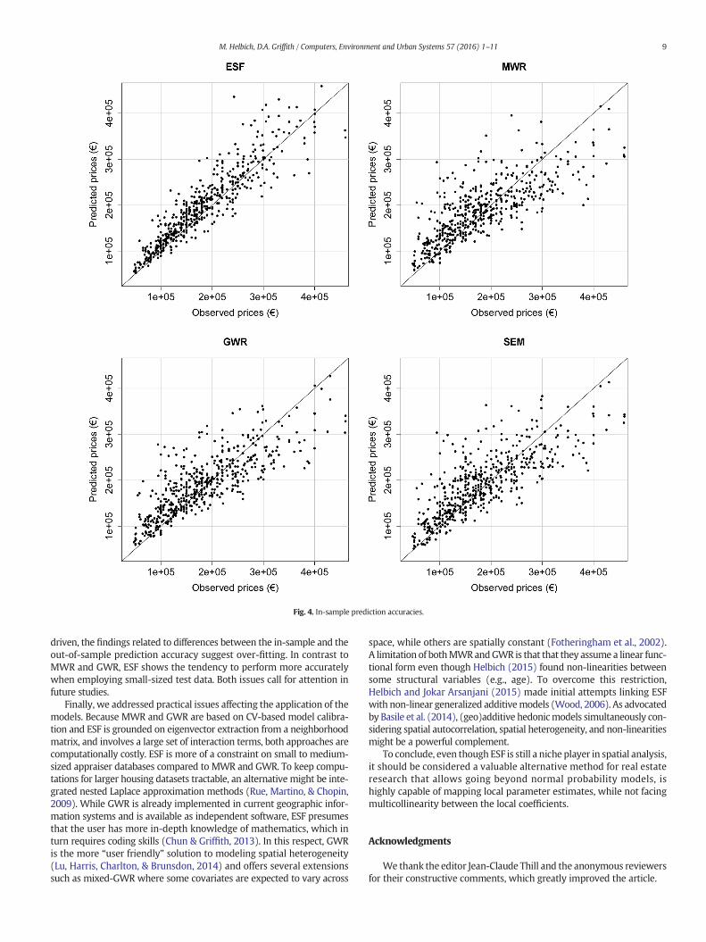
Fig. 4. In-sample prediction accuracies.

9M. Helbich, D.A. Griffith / Computers, Environment and Urban Systems 57 (2016) 1–11

driven, the findings related to differences between the in-sample and theout-of-sample prediction accuracy suggest over-fitting. In contrast toMWR and GWR, ESF shows the tendency to perform more accuratelywhen employing small-sized test data. Both issues call for attention infuture studies.

Finally, we addressed practical issues affecting the application of themodels. Because MWR and GWR are based on CV-based model calibra-tion and ESF is grounded on eigenvector extraction from a neighborhoodmatrix, and involves a large set of interaction terms, both approaches arecomputationally costly. ESF is more of a constraint on small to medium-sized appraiser databases compared to MWR and GWR. To keep compu-tations for larger housing datasets tractable, an alternative might be inte-grated nested Laplace approximation methods (Rue, Martino, & Chopin,2009). While GWR is already implemented in current geographic infor-mation systems and is available as independent software, ESF presumesthat the user has more in-depth knowledge of mathematics, which inturn requires coding skills (Chun & Griffith, 2013). In this respect, GWRis the more “user friendly” solution to modeling spatial heterogeneity(Lu, Harris, Charlton, & Brunsdon, 2014) and offers several extensionssuch as mixed-GWR where some covariates are expected to vary across

space, while others are spatially constant (Fotheringham et al., 2002).A limitation of bothMWRandGWR is that that they assume a linear func-tional form even though Helbich (2015) found non-linearities betweensome structural variables (e.g., age). To overcome this restriction,Helbich and Jokar Arsanjani (2015) made initial attempts linking ESFwith non-linear generalized additivemodels (Wood, 2006). As advocatedby Basile et al. (2014), (geo)additive hedonicmodels simultaneously con-sidering spatial autocorrelation, spatial heterogeneity, and non-linearitiesmight be a powerful complement.

To conclude, even though ESF is still a niche player in spatial analysis,it should be considered a valuable alternative method for real estateresearch that allows going beyond normal probability models, ishighly capable of mapping local parameter estimates, while not facingmulticollinearity between the local coefficients.

Acknowledgments

We thank the editor Jean-Claude Thill and the anonymous reviewersfor their constructive comments, which greatly improved the article.

Table 3Results of the predictive accuracy assessment.

Size test data In-sampleSpearman's ρ

LOOCV RMSE

1st QT Median 3rd QT 1st QT Median 3rd QT

20% test data ESF 0.919 0.924 0.930 0.260 0.276 0.333MWR 0.689 0.699 0.711 0.329 0.335 0.340GWR 0.697 0.706 0.716 0.327 0.332 0.336SEM 0.764 0.774 0.783 0.312 0.318 0.324

10% test data ESF 0.899 0.904 0.910 0.265 0.272 0.297MWR 0.694 0.699 0.706 0.332 0.336 0.338GWR 0.702 0.707 0.713 0.327 0.331 0.334SEM 0.765 0.770 0.775 0.317 0.319 0.323

Size test data Hold-out sampleSpearman's ρ

Hold-out sampleRMSE

1st QT Median 3rd QT 1st QT Median 3rd QT

20% test data ESF 0.448 0.509 0.551 0.585 0.656 0.829MWR 0.659 0.687 0.730 0.325 0.341 0.361GWR 0.668 0.699 0.737 0.322 0.336 0.355

10% test data SEM 0.638 0.684 0.725 0.331 0.351 0.371ESF 0.492 0.547 0.609 0.473 0.533 0.637MWR 0.643 0.689 0.740 0.309 0.332 0.362GWR 0.650 0.700 0.746 0.299 0.326 0.352SEM 0.620 0.687 0.729 0.321 0.346 0.371

10 M. Helbich, D.A. Griffith / Computers, Environment and Urban Systems 57 (2016) 1–11

References

Ahn, J., Byun, H., Oh, K., & Kim, T. (2012). Using ridge regression with genetic algorithmto enhance real estate appraisal forecasting. Expert Systems with Applications, 39(9),8369–8379.

Alberto, I., Beamonte, A., Gargallo, P., Mateo, P., & Salvador, M. (2010). Variable selectionin STAR models with neighbourhood effects using genetic algorithms. Journal ofForecasting, 29(8), 728–750.

Ali, K., Partridge, M., & Olfert, R. (2007). Can geographically weighted regressions improveregional analysis and policy making? International Regional Science Review, 30(3),300–329.

Anselin, L., & Arribas-Bel, D. (2013). Spatial fixed effects and spatial dependence in a singlecross-section. Papers in Regional Science, 92(1), 3–18.

Basile, R., et al. (2014). Modeling regional economic dynamics: Spatial dependence,spatial heterogeneity and nonlinearities. Journal of Economic Dynamics &Control, l48, 229–245.

Bitter, C., Mulligan, G., & Dall'erba, S. (2007). Incorporating spatial variation in housingattribute prices: A comparison of geographically weighted regression and the spatialexpansion method. Journal of Geographical Systems, 9(1), 7–27.

Bourassa, S., Cantoni, E., &Hoesli,M. (2010). Predictinghousepriceswith spatial dependence:A comparison of alternative methods. Journal of Real Estate Research, 32(2), 139–160.

Brunsdon, C., Charlton, M., & Harris, P. (2012). Living with collinearity in local regressionmodels. Spatial accuracy 2012, Florianópolis, Brazil.

Can, A. (1992). Specification and estimation of hedonic house price models. RegionalScience and Urban Economics, 22(3), 453–474.

Cassetti, E. (1972). Generating models by the expansion method: Applications to geo-graphical research. Geographical Analysis, 4(1), 81–91.

Cassetti, E. (1997). The expansion method, mathematical modeling, and spatial econo-metrics. International Regional Science Review, 20(1–2), 9–33.

Cho, S., Lambert, D., Kim, S., & Jung, S. (2009). Extreme coefficients in geographicallyweighted regression and their effects on mapping. GIScience & Remote Sensing,46(3), 273–288.

Chun, Y., & Griffith, D. (2013). Spatial statistics and geostatistics: Theory and applica-tions for geographic information science and technology. Thousand Oaks: SAGEPublications.

Cliff, A., & Ord, J. (1973). Spatial autocorrelation. London: Pion.de Jong, P., Sprenger, C., & van Veen, F. (1984). On extreme values ofMoran's I and Geary's

C. Geographical Analysis, 16(1), 17–24.Dubin, R. (1998). Spatial autocorrelation: A primer. Journal of Housing Economics, 7(4),

304–327.Farber, S., & Yeates, M. (2006). A comparison of localized regression models in a hedonic

house price context. Canadian Journal of Regional Science, 29(3), 405–420.Fik, T., Ling, D., &Mulligan, G. (2003).Modeling spatial variation in housing prices: A variable

interaction approach. Real Estate Economics, 31(4), 623–646.Fotheringham, S., Charlton, M., & Brunsdon, C. (1998). Geographically weighted regression:

A natural evolution of the expansion method for spatial data analysis. Environment andPlanning A, 30(11), 1905–1927.

Fotheringham, S., Charlton, M., & Brunsdon, C. (2002). Geographically weighted regression.The analysis of spatially varying relationships. Chichester: Wiley.

Gao, X., Asami, Y., & Chung, C. -J. (2006). An empirical evaluation of spatial regressionmodels. Computers & Geosciences, 32(8), 1040–1051.

Getis, A. (1990). Screening for spatial dependence in regression analysis. Papers in RegionalScience, 69(1), 69–81.

Getis, A. (2009). Spatial weights matrices. Geographical Analysis, 41(4), 404–410.Goldberg, D. (1989). Genetic algorithms in search, optimization and machine learning. Boston:

Addison-Wesley.Goodman, A., & Thibodeau, T. (2003). Housingmarket segmentation and hedonic prediction

accuracy. Journal of Housing Economics, 12(3), 181–201.Griffith, D. (2000). A linear regression solution to the spatial autocorrelation problem.

Journal of Geographical Systems, 2(2), 141–156.Griffith, D. (2008). Spatial-filtering-based contributions to a critique of geographically

weighted regression (GWR). Environment and Planning A, 40(11), 2751–2769.Griffith, D. (2012). Space, time, and space-time eigenvector filter specifications that

account for autocorrelation. Estadística Española, 54(177), 7–34.Griffith, D., & Peres-Neto, P. (2006). Spatial modeling in ecology: The flexibility of

eigenfunction spatial analyses. Ecology, 87(10), 2603–2613.Hagenauer, J., & Helbich, M. (2012). Mining urban land-use patterns from volunteered

geographic information by means of genetic algorithms and artificial neural networks.International Journal of Geographical Information Science, 26(6), 963–982.

Hastie, T., Tibshirani, R., & Friedman, J. (2009). The elements of statistical learning.Heidelberg:Springer.

Helbich, M. (2015). Do suburban areas impact house prices? Environment and Planning B:Planning and Design, 42(3), 431–449.

Helbich, M., & Jokar Arsanjani, J. (2015). Spatial eigenvector filtering for spatiotemporalcrime mapping and spatial crime analysis. Cartography and Geographic InformationScience, 42(2), 134–148.

Helbich, M., Brunauer, W., Hagenauer, J., & Leitner, M. (2013a). Data-driven regionalizationof housing markets. Annals of the Association of American Geographers, 103(4), 871–889.

Helbich, M., Brunauer, W., Vaz, E., & Nijkamp, P. (2014). Spatial heterogeneity in hedonichouse price models: The case of Austria. Urban Studies, 51(2), 390–411.

Helbich, M., Jochem, A., Mücke, W., & Höfle, B. (2013b). Boosting the predictive accuracyof urban hedonic house price models through airborne laser scanning. Computers,Environment and Urban Systems, 39, 81–92.

Jetz,W., Rahbek, C., & Lichstein, J. (2005). Local and global approaches to spatial data analysisin ecology. Global Ecology and Biogeography, 14(1), 97–98.

Kestens, Y., Theriault, M., & Des Rosiers, F. (2006). Heterogeneity in hedonic modeling ofhouse prices: Looking at buyers' households profiles. Journal of Geographical Systems,8(1), 61–96.

Kuntz, M., & Helbich, M. (2014). Geostatistical mapping of real estate prices: An empiricalcomparison of kriging and cokriging. International Journal of Geographical InformationScience, 29, 1904–1921.

Lancaster, K. (1966). A new approach to consumer theory. Journal of Political Economy,74(2), 132–157.

LeSage, J., & Pace, K. (2004). Models for spatially dependent missing data. Journal of RealEstate Finance and Economics, 29(2), 233–254.

LeSage, J., & Pace, K. (2009). Introduction to spatial econometrics. Boca Raton: CRC Press.Leung, Y., Mei, C. -L., & Zhang, W. -X. (2000). Statistical tests for spatial non-stationarity

based on the geographically weighted regression model. Environment and PlanningA, 32(1), 9–32.

Lu, B., Charlton, M., Harris, P., & Fotheringham, S. (2014a). Geographically weightedregression with a non-Euclidean distance metric: A case study using hedonichouse price data. International Journal of Geographical Information Science,27(4), 660–681.

Lu, B., Harris, P., Charlton, M., & Brunsdon, C. (2014b). The GWmodel R package: Furthertopics for exploring spatial heterogeneity using geographically weighted models.Geo-spatial Information Science, 17(2), 85–101.

Malpezzi, S. (2003). Hedonic pricing models: A selective and applied review. In T.O'Sullivan, & K. Gibb (Eds.), Housing economics and public policy (pp. 67–89). Oxford:Blackwell.

McMillen, D., & Redfearn, C. (2010). Estimation, interpretation, and hypothesis testing fornonparametric hedonic house price functions. Journal of Regional Science, 50(3),712–733.

Osland, L. (2010). An application of spatial econometrics in relation to hedonic houseprice modeling. Journal of Real Estate Research, 32(3), 289–320.

Pace, K., Barry, R., & Sirmans, C. (1998). Spatial statistics and real estate. Journal of RealEstate Finance and Economics, 17, 5–13.

Páez, A., Farber, S., & Wheeler, D. (2011). A simulation-based study of geographicallyweighted regression as a method for investigating spatially varying relationships.Environment and Planning A, 43(12), 2992–3010.

Páez, A., Fei, L., & Farber, S. (2008). Moving window approaches for hedonic priceestimation: An empirical comparison of modelling techniques. Urban Studies,45(8), 1565–1581.

Palm, R. (1978). Spatial segmentation of the urban housing market. Economic Geography,54(3), 210–221.

Patuelli, R., Schanne, N., Griffith, D., & Nijkamp, P. (2012). Persistence of regional unem-ployment: Application of a spatial filtering approach to local labor markets inGermany. Journal of Regional Science, 52(2), 300–323.

Pavlov, A. (2000). Space-varying regression coefficients: A semi-parametric approachapplied to real estate markets. Real Estate Economics, 28(2), 249–283.

Quigley, J. (1985). Consumer choice of dwelling, neighborhood and public services.Regional Science and Urban Economics, 15(1), 41–63.

Redfearn, C. (2009). How informative are average effects? Hedonic regression and amenitycapitalization in complex urban housingmarkets. Regional Science and Urban Economics,39(3), 297–306.

Reggiani, A., Nijkamp, P., & Sabella, E. (2001). New advances in spatial network modelling:Towards evolutionary algorithms. European Journal of Operational Research, 128(2),385–401.

Rosen, S. (1974). Hedonic prices and implicit markets: Product differentiation in purecompetition. Journal of Political Economy, 82(1), 34–55.

11M. Helbich, D.A. Griffith / Computers, Environment and Urban Systems 57 (2016) 1–11

Rue, H., Martino, S., & Chopin, N. (2009). Approximate Bayesian inference for latentGaussian models by using integrated nested Laplace approximations. Journal of theRoyal Statistical Society: Series B, 71(2), 319–392.

Schnare, A., & Struyk, R. (1976). Segmentation in urban housing markets. Journal of UrbanEconomics, 54(3), 146–166.

Scrucca, L. (2013). GA: A package for genetic algorithms in R. Journal of Statistical Software,53(4), 1–37.

Seya, H., Murakami, D., Tsutsumi, M., & Yamagata, Y. (2014). Application of LASSO to theeigenvector selection problem in eigenvector-based spatial filtering. GeographicalAnalysis (early view).

Sheppard, S. (1997). Hedonic analysis of housing market. In P. Chesire, & E. Mills (Eds.),Handbook of regional and urban economics, vol. 3. (pp. 1595–1635). Amsterdam:Elsevier.

Sunding, D., & Swoboda, A. (2010). Hedonic analysis with locally weighted regression: Anapplication to the shadow cost of housing regulation in Southern California. RegionalScience and Urban Economics, 40(6), 550–573.

Tiefelsdorf, M., & Boots, B. (1995). The exact distribution of Moran's I. Environment andPlanning A, 27(6), 985–999.

Tiefelsdorf, M., & Griffith, D. (2007). Semiparametric filtering of spatial autocorrelation:The eigenvector approach. Environment and Planning A, 39(5), 1193–1221.

Vidaurre, D., Bielza, C., & Larrañaga, P. (2012). Lazy lasso for local regression.Computational Statistics, 27(3), 531–550.

Wheeler, D. (2009). Simultaneous coefficient penalization and model selection ingeographically weighted regression: The geographically weighted lasso. Environmentand Planning A, 41(3), 722–742.

Wheeler, D., & Tiefelsdorf, M. (2005). Multicollinearity and correlation among localregression coefficients in geographically weighted regression. Journal of GeographicalSystems, 7(2), 161–187.

Wood, S. (2006). Generalized additive models: An introduction with R. Boca Raton: CRCPress.