Spatial Network Modeling for Databases

Virupaksha Kanjilal & Markus Schneider∗University of Florida

Department of Computer & Information Science & EngineeringGainesville, Florida, USA

{vk4, mschneid}@cise.ufl.edu

ABSTRACTSpatial networks like transportation, power, and pipelinenetworks are a ubiquitous spatial concept in everyday lifeand play an important role for navigational and routing pur-poses. Database support for large spatial networks in orderto represent, store, query, and manipulate them is rare. Ourpaper aims to provide the beginning of a conceptual, ab-stract, and formal model of spatial networks, called SpatialNetwork Algebra (SNA), that includes types and operationsand is supposed to serve as a specification for their later im-plementation in spatial database systems and GIS. Finally,we show how our spatial network concepts can be embeddedinto an SQL-like query language.

1. INTRODUCTIONSpatial networks like road networks connecting cities, rail

networks connecting railway stations, pipeline networks car-rying water to our houses are ubiquitous in everyday life.Spatial networks are spatially embedded graphs created bythe interconnection of spatial elements such as spatial linesand spatial points. Apart from their use in spatially ori-ented disciplines like geography, cartography, GeographicalInformation Systems (GIS), and spatial databases systems,spatial networks also find application in transport and nav-igation as in GPS devices or in traffic forecasting models.Database support is necessary to efficiently utilize the

large volumes of data in any spatial network. But till now,database support for spatial networks is rare and neglected.Available GIS implementations of spatial networks only usethe database system to deliver the basic components of thenetwork so that an in-memory network can be built in amiddleware layer. This approach fails to take advantage ofthe benefits provided by the database system like query pro-cessing, concurrency control, and transaction management.To integrate spatial networks in a database context as a

first class citizen, we need a formal model of spatial networks

∗This work was partially supported by the National ScienceFoundation under grant number NSF-IIS-0812194.

Permission to make digital or hard copies of all or part of this work forpersonal or classroom use is granted without fee provided that copies arenot made or distributed for profit or commercial advantage and that copiesbear this notice and the full citation on the first page. To copy otherwise, torepublish, to post on servers or to redistribute to lists, requires prior specificpermission and/or a fee.SAC’11 March 21-25, 2011, TaiChung, Taiwan.Copyright 2011 ACM 978-1-4503-0113-8/11/03 ...$10.00.

which will serve as the specification for any implementation.The goal of this paper is to create a data model for networksembedded in space with its own type definitions. Due tospace constraints, we will only introduce a few of the basicoperations and predicates on them. Finally we show a fewqueries in an SQL-like query language that take advantageof the operations and predicates on a spatial network. Thismodel is a part of a complete algebra for spatially embeddedgraphs called the Spatial Network Algebra (SNA).

In our approach, points in the Euclidean plane which area part of the network have thematic properties associated tothem. The thematic properties distinguish components of anetwork, i.e., all the points with equal thematic propertiesbelong to the same network component. Interior and exte-rior points of a network can be distinguished based on thethematic properties. In particular, this approach enables usto consider attributes of single points (space based view)but also provides access to collections of points having equalattributes (object based view).

Section 2 gives an overview of the various approaches tomodeling spatial network. Section 3 introduces the SpatialNetwork Algebra as our model of spatial networks. Sec-tion 4 defines a few important operations and predicateson our spatial network model. In Section 5 we introduce anSQL-like query language that can be used to create or queryspatial networks.

2. RELATED WORKIn this section, we confine ourselves exclusively to model-

ing approaches to spatial networks. A reasonable and popu-lar concept is to model spatial networks as planar graphs inorder to capture their structure and connectivity. Querieslike the shortest path or the maximum flow can be directlymapped to well known graph problems for which algorithmsexist. For example, the shortest path problem may be solvedby Dijkstra’s algorithm, and the maximum flow problem canbe solved by the Ford Fulkerson algorithm. This approach tomodeling networks has been taken in [4] and [6]. The modelin [4] has been designed for embedding graphs in databasesand not specifically for spatial graphs. The work in [6]models road networks by defining road components basedon their properties and the potential actions they may per-form. The authors term this as an“affordance-based”theoryof networks. Though graph modeling has some advantages,real world networks are too complex to be represented bysimple graphs [5].

Routes are essential concepts in a spatial network, as themodels in [3, 1] show. Routes correspond to paths in a graph

and to roads in a transportation network. In these models, anetwork can be explicitly stored in a database which enablesthe formulation of powerful queries and efficient execution.However these approaches cannot store and represent thethematic attributes of the network components. The small-est network unit in these cases is a road or a junction. Inour model, we assume every point of the network is markedwith its thematic attributes, and we aggregate all pointswith equal attributes to form network components.

3. THE SPATIAL NETWORK MODELIn this section we introduce our model of spatial networks.

We begin by providing an intuitive description of spatialnetworks in Section 3.1. In Section 3.2 we give the formaldefinitions of network components and the network itself.

3.1 What are Spatial Networks?Spatial networks are a ubiquitous spatial concept. We use

transportation networks like road networks for cars, buses,and taxis or railway networks for trains and metro everyday. Water pipelines and power networks supply our houseswith valuable resources. If we abstract from these particu-lar kinds of networks, we can say that the primary purposeof spatial networks is to provide a spatially constrained en-vironment for materials (in the broadest sense) to move orflow through them.From a modeling perspective, a spatial network can be

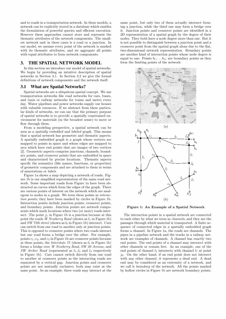
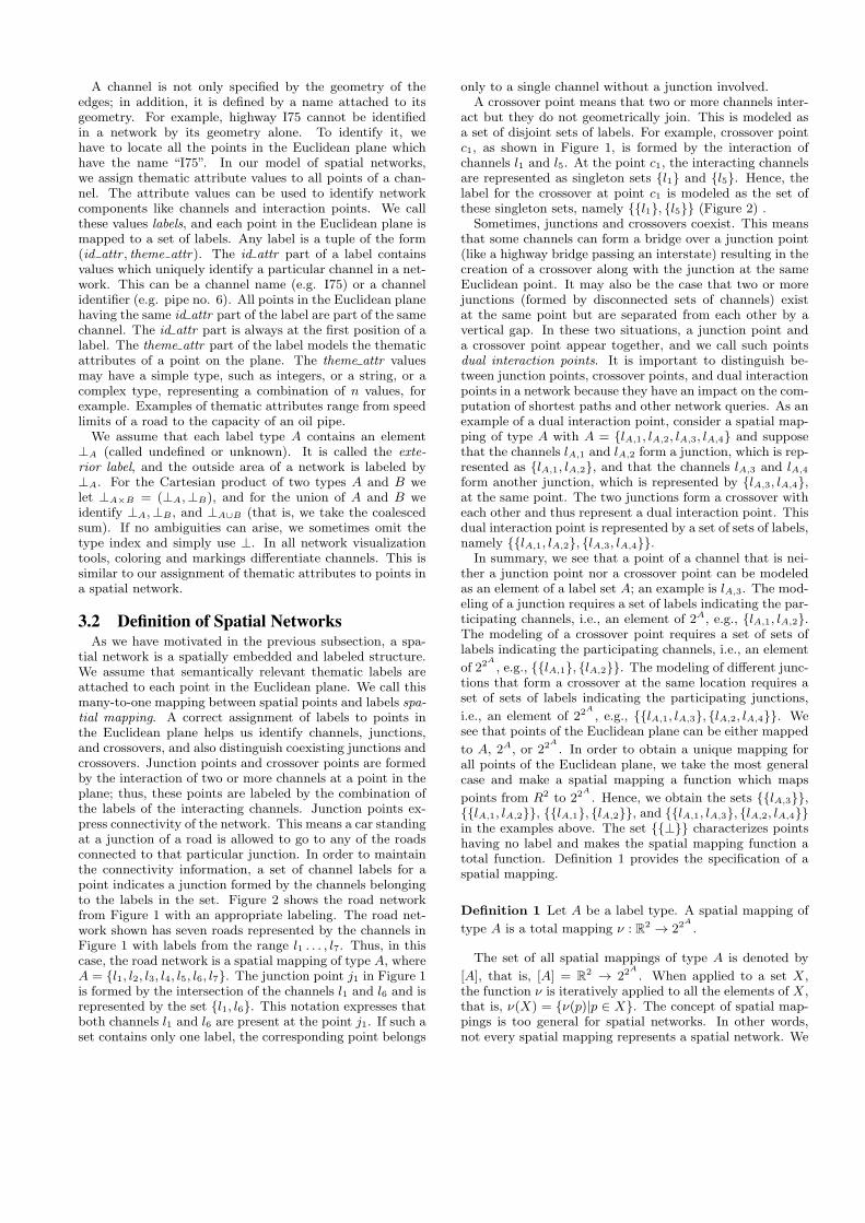
seen as a spatially embedded and labeled graph. This meansthat a spatial network has geometric and thematic aspects.A spatially embedded graph is a graph whose vertices aremapped to points in space and whose edges are mapped toarcs which have end points that are images of two vertices[2]. Geometric aspects comprise junctions, channels, bound-ary points, and crossover points that are embedded in spaceand characterized by precise locations. Thematic aspectsspecify the semantics (like names, functions, or properties)of geometric components and are attached to them in termsof annotations or labels.Figure 1a shows a map depicting a network of roads. Fig-

ure 1b is our simplified representation of the same road net-work. Some important roads from Figure 1a have been ab-stracted as curves which form the edges of the graph. Thereare various points of interest on the network which are anal-ogous to nodes in a graph. We term these points as interac-tion points; they have been marked by circles in Figure 1b.Interaction points include junction points, crossover points,and boundary points. Junction points are network compo-nents which mark locations where two (or more) roads inter-sect. The point j1 in Figure 1b is a junction because at thispoint the roads W Newberry Road (shown as l1 in Figure 1b)and SW 75th street (shown as l6 in Figure 1b) intersect. Carscan switch from one road to another only at junction points.This is opposed to crossover points where two roads interactbut one road forms a bridge over the other. For example,points c1, c2, and c3 in Figure 1b are crossover points becauseat these points, the Interstate 75 (shown as l5 in Figure 1b)forms a bridge over W Newberry Road, SW 20 Avenue, andSW Archer Road (represented as l1, l3 and l4 respectivelyin Figure 1b). Cars cannot switch directly from one roadto another at crossover points as the interacting roads areseparated by a vertical gap. Junction points and crossoverpoints are not mutually exclusive; both may exist at thesame point. As an example, three roads may interact at the

same point, but only two of them actually intersect form-ing a junction, while the third one may form a bridge overit. Junction points and crossover points are identified in a2D representation of a spatial graph by the degree of theirnodes. They both have a node degree more than one. But itis not possible to distinguish between a junction point and acrossover point from the spatial graph alone due to the flat,two-dimensional network representation. Boundary pointsare another kind of interaction points whose node degree isequal to one. Points b1, . . . b11 are boundary points as theyform the limiting points of the network.

(a)

(b)

Figure 1: An Example of a Spatial Network

The interaction points in a spatial network are connectedto each other by what we term as channels, and they are thepassages through which material is transported. A finite se-quence of connected edges in a spatially embedded graphforms a channel. In Figure 1a, the roads are channels. Thepipes in a pipeline network and the tracks in a railway net-work are examples of channels. A channel has exactly twoend points. The end points of a channel may intersect withother channels or remain free. As an example, one of theend points of channel l3 intersects with channel l7 at pointj6. On the other hand, if an end point does not intersectwith any other channel, it represents a dead end. A deadend may be considered as an extremity of a network, andwe call it boundary of the network. All the points markedby hollow circles in Figure 1b are network boundary points.

A channel is not only specified by the geometry of theedges; in addition, it is defined by a name attached to itsgeometry. For example, highway I75 cannot be identifiedin a network by its geometry alone. To identify it, wehave to locate all the points in the Euclidean plane whichhave the name “I75”. In our model of spatial networks,we assign thematic attribute values to all points of a chan-nel. The attribute values can be used to identify networkcomponents like channels and interaction points. We callthese values labels, and each point in the Euclidean plane ismapped to a set of labels. Any label is a tuple of the form(id attr , theme attr). The id attr part of a label containsvalues which uniquely identify a particular channel in a net-work. This can be a channel name (e.g. I75) or a channelidentifier (e.g. pipe no. 6). All points in the Euclidean planehaving the same id attr part of the label are part of the samechannel. The id attr part is always at the first position of alabel. The theme attr part of the label models the thematicattributes of a point on the plane. The theme attr valuesmay have a simple type, such as integers, or a string, or acomplex type, representing a combination of n values, forexample. Examples of thematic attributes range from speedlimits of a road to the capacity of an oil pipe.We assume that each label type A contains an element

⊥A (called undefined or unknown). It is called the exte-rior label, and the outside area of a network is labeled by⊥A. For the Cartesian product of two types A and B welet ⊥A×B = (⊥A,⊥B), and for the union of A and B weidentify ⊥A,⊥B , and ⊥A∪B (that is, we take the coalescedsum). If no ambiguities can arise, we sometimes omit thetype index and simply use ⊥. In all network visualizationtools, coloring and markings differentiate channels. This issimilar to our assignment of thematic attributes to points ina spatial network.

3.2 Definition of Spatial NetworksAs we have motivated in the previous subsection, a spa-

tial network is a spatially embedded and labeled structure.We assume that semantically relevant thematic labels areattached to each point in the Euclidean plane. We call thismany-to-one mapping between spatial points and labels spa-tial mapping. A correct assignment of labels to points inthe Euclidean plane helps us identify channels, junctions,and crossovers, and also distinguish coexisting junctions andcrossovers. Junction points and crossover points are formedby the interaction of two or more channels at a point in theplane; thus, these points are labeled by the combination ofthe labels of the interacting channels. Junction points ex-press connectivity of the network. This means a car standingat a junction of a road is allowed to go to any of the roadsconnected to that particular junction. In order to maintainthe connectivity information, a set of channel labels for apoint indicates a junction formed by the channels belongingto the labels in the set. Figure 2 shows the road networkfrom Figure 1 with an appropriate labeling. The road net-work shown has seven roads represented by the channels inFigure 1 with labels from the range l1 . . . , l7. Thus, in thiscase, the road network is a spatial mapping of type A, whereA = {l1, l2, l3, l4, l5, l6, l7}. The junction point j1 in Figure 1is formed by the intersection of the channels l1 and l6 and isrepresented by the set {l1, l6}. This notation expresses thatboth channels l1 and l6 are present at the point j1. If such aset contains only one label, the corresponding point belongs

only to a single channel without a junction involved.A crossover point means that two or more channels inter-

act but they do not geometrically join. This is modeled asa set of disjoint sets of labels. For example, crossover pointc1, as shown in Figure 1, is formed by the interaction ofchannels l1 and l5. At the point c1, the interacting channelsare represented as singleton sets {l1} and {l5}. Hence, thelabel for the crossover at point c1 is modeled as the set ofthese singleton sets, namely {{l1}, {l5}} (Figure 2) .

Sometimes, junctions and crossovers coexist. This meansthat some channels can form a bridge over a junction point(like a highway bridge passing an interstate) resulting in thecreation of a crossover along with the junction at the sameEuclidean point. It may also be the case that two or morejunctions (formed by disconnected sets of channels) existat the same point but are separated from each other by avertical gap. In these two situations, a junction point anda crossover point appear together, and we call such pointsdual interaction points. It is important to distinguish be-tween junction points, crossover points, and dual interactionpoints in a network because they have an impact on the com-putation of shortest paths and other network queries. As anexample of a dual interaction point, consider a spatial map-ping of type A with A = {lA,1, lA,2, lA,3, lA,4} and supposethat the channels lA,1 and lA,2 form a junction, which is rep-resented as {lA,1, lA,2}, and that the channels lA,3 and lA,4

form another junction, which is represented by {lA,3, lA,4},at the same point. The two junctions form a crossover witheach other and thus represent a dual interaction point. Thisdual interaction point is represented by a set of sets of labels,namely {{lA,1, lA,2}, {lA,3, lA,4}}.

In summary, we see that a point of a channel that is nei-ther a junction point nor a crossover point can be modeledas an element of a label set A; an example is lA,3. The mod-eling of a junction requires a set of labels indicating the par-ticipating channels, i.e., an element of 2A, e.g., {lA,1, lA,2}.The modeling of a crossover point requires a set of sets oflabels indicating the participating channels, i.e., an element

of 22A

, e.g., {{lA,1}, {lA,2}}. The modeling of different junc-tions that form a crossover at the same location requires aset of sets of labels indicating the participating junctions,

i.e., an element of 22A

, e.g., {{lA,1, lA,3}, {lA,2, lA,4}}. Wesee that points of the Euclidean plane can be either mapped

to A, 2A, or 22A

. In order to obtain a unique mapping forall points of the Euclidean plane, we take the most generalcase and make a spatial mapping a function which maps

points from R2 to 22A

. Hence, we obtain the sets {{lA,3}},{{lA,1, lA,2}}, {{lA,1}, {lA,2}}, and {{lA,1, lA,3}, {lA,2, lA,4}}in the examples above. The set {{⊥}} characterizes pointshaving no label and makes the spatial mapping function atotal function. Definition 1 provides the specification of aspatial mapping.

Definition 1 Let A be a label type. A spatial mapping of

type A is a total mapping ν : R2 → 22A

.

The set of all spatial mappings of type A is denoted by

[A], that is, [A] = R2 → 22A

. When applied to a set X,the function ν is iteratively applied to all the elements of X,that is, ν(X) = {ν(p)|p ∈ X}. The concept of spatial map-pings is too general for spatial networks. In other words,not every spatial mapping represents a spatial network. We

Figure 2: A Spatial Network [A] with labels

have to impose certain restrictions on spatial mappings asdescribed in the following. The idea is to infer and dis-tinguish channels, junctions, and crossovers from the labelinformation. Points which have a label other than {{⊥}}belong to a channel. A crossover point is indicated by a setcontaining at least two sets of channel labels. To identifyjunction points, we look into each set of labels. If any one ofthe sets has more than one channel label, it means that thechannels which belong to those labels form a junction. Def-inition 2 identifies channels, junction points, and crossoverpoints in a spatial mapping.

Definition 2 Let ν be a spatial mapping of type A. Then

(i) L(ν) = {p|p ∈ R2 ∧ ν(p) 6= {{⊥}}} (channels)(ii) J(ν) = {p|p ∈ R2 ∧ (∃ l ∈ ν(p) : |l| > 1)}

(junctions)(iii) C(ν) = {p|p ∈ R2 ∧ |ν(p)| > 1} (crossover)

L(ν) contains all the points in the Euclidean plane whichare part of a channel. Individual channels can be identifiedby the label information, as the id attr part of the labeluniquely identifies a channel. All the points of the samechannel have the same id attr part in their label. Thus,each channel may be distinguished by grouping the pointsin L(ν) by the id attr part of the label. This necessitates alook into the labels and an extraction of parts from them.We can assume that an element of the label type A is asequence of label attribute values and that each such valueis of a (possibly different) set Ai. That is, A =×k

i=1Ai =

A1 × . . . × Ak. Let I = {1, . . . , k}, S = {j1, . . . , jn}, andS ⊆ I. To extract selected attribute values from a label, wedefine a projection operator Π as follows:

ΠS :×i∈IAi →×j∈S

Aj

with ΠS(a1, . . . , ak) = (aj1 , . . . , ajn).Next we define a function called Id Attr to extract all the

id attr label parts actually present in a spatial mapping. Ittakes as argument a spatial mapping ν of type A and com-putes the set of all id attr values by using the projectionoperator Π. As the id attr attribute is assumed to be al-ways the first attribute a1 in a label, we use Π{1} to extractits value. Further, we generalize function applications from

elements to sets of elements. Let f : X → Y be a function,and let B ⊆ X. Then we allow to use the notation f(B)which is given as f(B) = {f(x) |x ∈ B}. This is here ap-plied to a spatial mapping ν. The function Id Attr is nowdefined for ν ∈ [A] as:

Id Attr(ν) = {Π{1}(l) | s ∈ ν(L(ν)), e ∈ s, l ∈ e}

Each channel has a unique id attr value; thus, all pointswhich belong to the same channel have the same id attrvalue in their labels. Definition 3 identifies all channelsin a spatial mapping by defining the two functions Chan-nel and Channels. The function Channel gets an id attrvalue as input and determines all points in the Euclideanplane that have this value in their labels and thus form aparticular channel. The function Channels gets a spatialmapping as input and collects all channels by iterating overall of its id attr values Points representing junction pointsor crossover points are part of interacting channels; hence,they appear in more than one channel.

Definition 3 Let ν be a spatial mapping of type A, and letl ∈ Id Attr(ν). Then

(i) Channel(l) = {p | p ∈ L(ν) ∧∃ s ∈ ν(p) ∃ e ∈ s : Π{1}(e) = l}

(ii) Channels(ν) = {Channel(l) | l ∈ Id Attr(ν)}

For the definition of a spatial network, we have to con-sider its underlying line-shaped geometric structures. Thisrequires the concept of a simple line which we give in Defi-nition 4.

Definition 4 The set sline of all simple lines in the Eu-clidean plane is defined as:

sline = {L ⊂ R2 |(i) ∃ f : [0, 1] → R2 : L = f([0, 1])(ii) f is a continuous mapping(iii) |f([0, 1])| > 1(iv) ∀ a, b ∈]0, 1[, a 6= b : f(a) 6= f(b)(v) ∀ a ∈ {0, 1} ∀ b ∈]0, 1[: f(a) 6= f(b)}

Conditions (i) and (ii) require the existence of a continu-ous function that generates the simple line. Condition (iii)avoids the anomaly that all elements of the unit interval aremapped to the same point. Condition (iv) states that a sim-ple line is not allowed to be self-intersecting. Condition (v)requires that a simple line is not self-touching.

We are now able to define a spatial network of type A asa special spatial mapping of type A (Definition 5).

Definition 5 A spatial network of type A is a spatial map-ping ν of type A such that

(i) ∀L ∈ Channels(ν) : L ∈ sline(ii) ∀ j ∈ J(ν) : j ∈ L(ν)(iii) ∀ c ∈ C(ν) : c ∈ L(ν)(iv) ∀ c ∈ C(ν) ∀ s1, s2 ∈ ν(c) ∀ l1 ∈ s1 ∀ l2 ∈ s2 :

Π{1}(l1) 6= Π{1}(l2)

Condition (iv) states that, in case of a crossover, the par-ticipating channels and/or junctions must be different sincethey cannot be physically present at more than one junction.This means that labels like {{l5}, {l5}} or {{l1, l5}, {l3, l5}}

are invalid. The condition checks whether the id attr valuesof the channels and/or junctions at each crossover point aredisjoint.We do not specify constraining topological relationships

between different channels of a spatial network. This meansthat different channels may meet, partially overlap, or onechannel may be contained in another channel. For example,in a road network, many roads carry several names. Thisis, for instance, the case for U.S. Route 441 which is a spurroute of U.S. Route 41.A channel L with a describing function fL : [0, 1] → R2

has two end points fL(0) and fL(1). Dual interaction points,represented by D(ν), indicate the co-existence of junctionsand crossovers. That is, D(ν) = J(ν) ∩ C(ν). If D(ν) = ∅holds, the spatial network does not have dual interactionpoints. If additionally C(ν) 6= ∅ holds, this means thatcrossover points are passed by single channels.The boundary points of a spatial network ν are those end

points of the channels that are not shared by other channels.Let Channels(ν) = {L1, . . . , Ln} that are described by func-tions fL1 , . . . , fLn . Let E(ν) =

∪ni=1{fLi(0), fLi(1)} be the

set of end points of all channels of ν. The set S(ν) ⊂ E(ν)of those points that are shared by more than one channel isgiven as

S(ν) = {p ∈ E(ν) |card({fLi | 1 ≤ i ≤ n ∧ fLi(0) = p})+card({fLi | 1 ≤ i ≤ n ∧ fLi(1) = p}) 6= 1}

Then the boundary points B(ν) are given as B(ν) =E(ν)− S(ν).

4. OPERATIONS ON SPATIAL NETWORKSA large number of interesting operations on spatial net-

works can be designed which assist in posing queries on spa-tial networks. Here we only describe a few of them includ-ing Routes (Section 4.1), Length (Section 4.2), and Short-estRoute (Section 4.3), which are classical network opera-tions.

4.1 Routes between Two Network PointsA route is a course (way, path, connection) one can take in

order to reach a second location from a first location. Givena spatial network, a route connects two points of the networkthrough an alternating sequence of channels and junctionsof the same network. A route between the two cities Atlantaand Gainesville is an example. Finding routes is an impor-tant feature of spatial network applications as the locationsof moving objects in a network are stored with respect to aparticular route. There can be possibly a large number ofroutes between two points in a network. We consider routesto be spatial networks with certain constraints. As a routeconnects two points p and q, the route starts at p and endsat q; i.e., p and q are the boundary points of the spatial net-work which represents a route. To prevent any discontinuityin the route, it can only have exactly two boundary points.In our model, we define an operator called Routes which

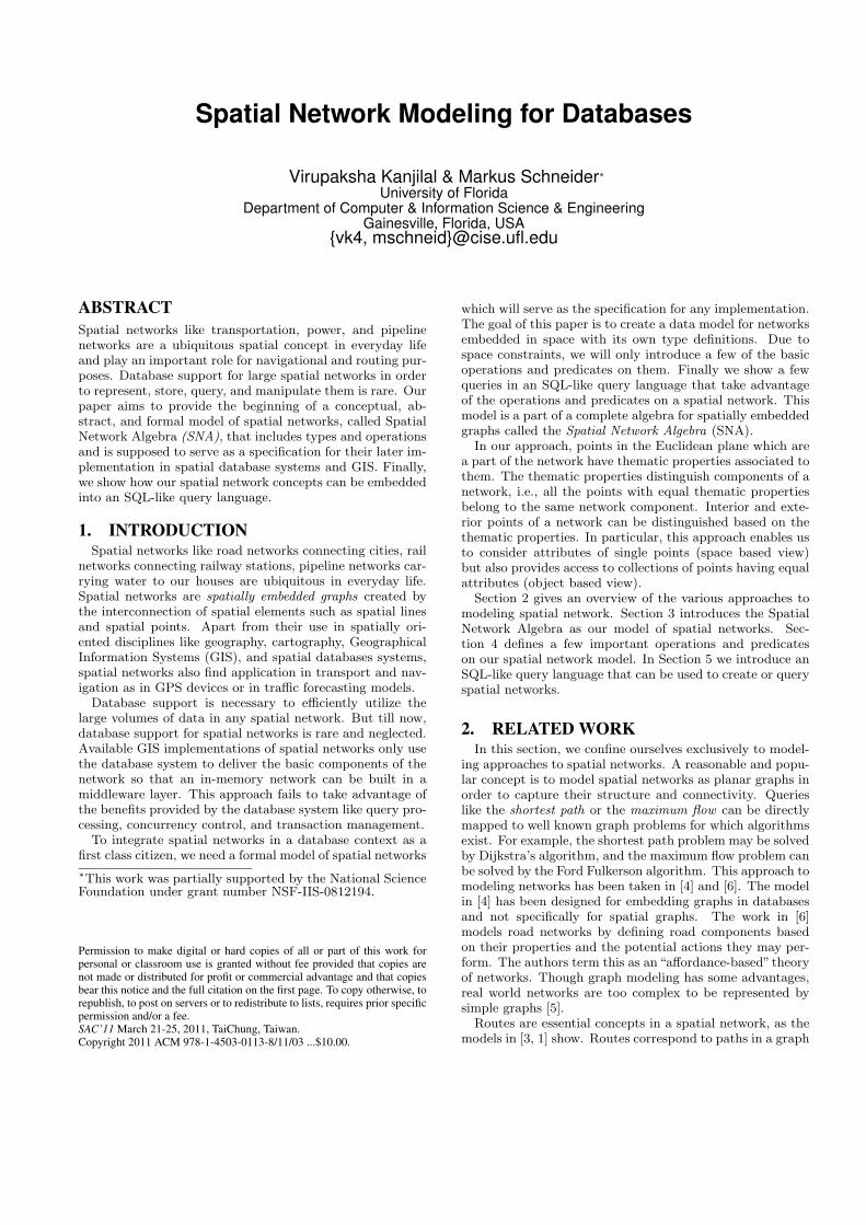
takes two points inside a spatial network and creates theset of all possible connections between them. The signatureof the Routes operator is Routes : [A] × R2 × R2 → 2[A].This operator returns the set of all spatial subnetworks rep-resenting routes between two selected points over a givenspatial network. All points of each returned spatial net-work, i.e., route, are a subset of the points of the original

network. Figure 3 shows the resulting routes when the oper-ation Routes(ν, j2 , j6 ) is performed on the network depictedin Figure 2 to calculate the paths from j2 to j6. Given aspatial network ν : [A] and two points p, q ∈ L(ν), we definethe Routes operator as

Routes(ν, p, q) = {ν′ | (i) ν′ : [A] is a spatial network(ii) L(ν′) ⊆ L(ν)(iii) ∀ l ∈ ν′(J(ν′)) : |l| = 2(iv) p, q ∈ B(ν′)(v) |B(ν′)| = 2}

Condition (i) states that every route is a spatial network.Condition (ii) ensures that every route ν′ is a subnetwork ofν. Condition (iii) requires that each junction of a route musthave a degree of exactly two. Condition (iv) states that pand q are boundary points of the route ν′. Condition (v)ensures that p and q are the only boundary points of ν′.

(a) (b)

(c)

Figure 3: The routes returned by executingRoutes(ν, j2 , j6 ) on the spatial network shown in Fig-ure 1b

4.2 Length of a ChannelLength is an important operator which calculates the length

of a channel. It yields a real value as a result. The Lengthoperator has the signature [A] → R. But only channels areallowed as input parameters. A channel must be integrableand bounded. This is always the case as the definition ofchannels requires that a channel is continuous and the de-scribing function is bounded in the interval [0,1]. To calcu-late the length, we divide the entire channel into infinitesi-mally small chord approximations and integrate them. Letus consider a channel L ∈ Channels(ν) with a describingfunction fL and the point set fL([0, 1]). The Length opera-tor is defined as

Length(L) =∫ fL(1)

fL(0)

√1 + (∂fL(x)/∂x)2∂x

This method may also be used to calculate the length be-tween any two points in the same channel. Here we simplyintegrate from the first point in the channel to the secondpoint in the channel. Consider again a channel L as de-scribed above, and the two points p = fL(a) and q = fL(b)

with a, b ∈ [0, 1]. We define a modified Length operator withthe signature Length : [A]× [0, 1]× [0, 1] → R as

Length(L, a, b) =∫ fL(b)

fL(a)

√1 + (∂fL(x)/∂x)2∂x

Another variation of the length operator is an extension ofthe first version with the same signature Length : [A] → R.But in this case, the length operator takes a complete spatialnetwork ν : [A] as argument and sums up the lengths of allthe channels in the spatial network. It is defined as

Length(ν) =∑

L∈Channels(ν)

Length(L)

4.3 Shortest RouteOne of the classical queries in a spatial network is the

shortest route (path) query. The task is to find a route be-tween two points in a network which has the least distanceamong all routes between the two points. Shortest routequeries are used to automatically find driving directions be-tween physical locations, e.g., between two cities. The Short-estRoute operator finds such a shortest route between twopoints p, q ∈ L(ν) in a network ν : [A]. The signature of thisoperator is ShortestRoute : [A]×R×R → [A]. Its definitionis given as

ShortestRoute(ν, p, q) = {sr |(i) sr ∈ Routes(ν, p, q)(ii) ∀ r ∈ Routes(ν, p, q) : Length(r) ≥ Length(sr)}

This operator checks all the routes between p and q andcompares their length. It chooses the route with the smallestlength as the shortest route. Since there could be severalshortest paths, it returns all of them in a set.

5. SPATIAL NETWORK QUERY LANGUAGEIn this section, we introduce an SQL-like query language

for spatial networks. We call the language Spatial NetworksQuery Language (SNQL). We assume that a database hasbeen created which holds spatial networks natively in it.Consider a national highway system represented as a spatialnetwork. A traveler wants to drive from Gainesville to At-lanta. The main aim of the traveler is to reach Atlanta inthe least amount of time. This means that he would like totravel on the route with the shortest length. Assuming wehave a network containing the national highways, this querymay be formulated as

select ShortestRoute(Gainesville, Atlanta) as srfrom NationalHighway

Sometimes the shortest route may not necessarily be theleast time taking route. There might be congestions andother causes of delay along this route. Hence, a travelermight be more interested in having a set of possible routesfrom Gainesville to Atlanta. He may then choose his pre-ferred route based on various other considerations like speedlimits and congestions. This may be formulated in a query.But the number of possible paths from Gainesville to At-lanta might be large. Thus the query should have a limit onthe number of routes it will return. In this particular case,we restrict the network distance of the paths to not morethan 500 miles. The query is as follows:

select Routes(Gainesville, Atlanta) as srfrom NationalHighwaywhere Length(sr) < 500

In the next query, the select clause is used to project out aparticular label attribute from the network. For example, aquery to find the average speed of the route from Gainesvilleto Atlanta could be formulated as follows:

select avg(speed limit)from (select ShortestRoute(Gainesville, Atlanta)

from NationalHighway)

This query finds the shortest route between Gainesvilleand Atlanta from the National Highway network in the innerquery, and then uses the aggregate function avg to calculatethe average of all values of the label attribute speed limitwith respect to the determined route. The label attribute isassumed to belong to the theme attr part (see Section 3.1)of the label type of the network NationalHighway.

6. CONCLUSIONS AND FUTURE WORKThis paper introduces and provides an overview of a for-

mal data model for spatial networks that serves as a spec-ification for a later implementation and integration in spa-tial (network) databases, Geographic Information Systems,transportation systems, and navigation systems. The datamodel is accompanied by some common operations, and theSpatial Networks Query Language (SNQL) demonstrateshow the operations may be used in a database context.

This paper is the beginning of a larger effort to createa Spatial Networks Algebra (SNA) that can model a broadrange of spatial networks and will have a comprehensive col-lection of operations and predicates defined on them. TheSpatial Networks Algebra will later be combined with spatialpartitions to create a Map Algebra.

7. REFERENCES[1] M. Erwig and R. H. Guting. Explicit Graphs in a

Functional Model for Spatial Databases. IEEETransactions on Knowledge and Data Engineering,6(5):787–804, 1994.

[2] T. Fleming and B. Mellor. An Introduction to VirtualSpatial Graph Theory. In Int. Workshop on KnotTheory for Scientific Objects, 2007.

[3] H. Guting, T. de Almeida, and Z. Ding. Modeling andQuerying Moving Objects in Networks. The VLDBJournal, 15(2):165–190, 2006.

[4] R. Guting. GraphDB: Modeling and Querying Graphsin Databases. 20th Int. Conf. on Very Large Databases,pages 297–308, 1994.

[5] C. S. Jensen, T. B. Pedersen, L. Speicys, and I. Timko.Data Modeling for Mobile Services in the Real World.In Advances in Spatial and Temporal Databases, pages1–9. Springer-Verlag, 2003.

[6] S. Scheider and W. Kuhn. Road Networks and TheirIncomplete Representation by Network Data Models. In5th Int. Conf. on Geographic Information Science(GIScience), pages 290–307. Springer-Verlag, 2008.